Catalyst for Gradient-based Nonconvex Optimization

Courtney Paquette Hongzhou Lin Dmitriy Drusvyatskiy

Lehigh University Massachusetts Institute of Technology University of Washington

Julien Mairal Zaid Harchaoui

Inria University of Washington

Abstract

We introduce a generic scheme to solve non-

convex optimization problems using gradient-

based algorithms originally designed for mini-

mizing convex functions. Even though these

methods may originally require convexity to

operate, the proposed approach allows one

to use them without assuming any knowl-

edge about the convexity of the objective.

In general, the scheme is guaranteed to pro-

duce a stationary point with a worst-case ef-

ﬁciency typical of ﬁrst-order methods, and

when the objective turns out to be convex,

it automatically accelerates in the sense of

Nesterov and achieves near-optimal conver-

gence rate in function values. We conclude

the paper by showing promising experimental

results obtained by applying our approach to

incremental algorithms such as SVRG and

SAGA for sparse matrix factorization and for

learning neural networks.

1 Introduction

We consider optimization problems of the form

min

x∈R

(

f(x) ,

i=1

(x) + ψ(x)

)

. (1)

Here, we set

R ∪ {∞}

, each function

: R

→ R

is smooth, and the regularization

ψ : R

→

may

be nonsmooth. By considering extended-real-valued

functions, this composite setting also encompasses con-

strained minimization by letting

be the indicator

function of computationally tractable constraints on

Proceedings of the 21

International Conference on Artiﬁ-

cial Intelligence and Statistics (AISTATS) 2018, Lanzarote,

Minimization of a regularized empirical risk objective

of form (1) is central in machine learning. Whereas a

signiﬁcant amount of work has been devoted to this

setting for convex problems, leading in particular to fast

incremental algorithms [see, e.g.,

the question of minimizing eﬃciently (1) when the

functions

and

may be nonconvex is still largely

open today.

Yet, nonconvex problems in machine learning are of

utmost interest. For instance, the variable

may rep-

resent the parameters of a neural network, where each

term

(

) measures the ﬁt between

and a data point

indexed by

, or (1) may correspond to a nonconvex

matrix factorization problem (see Section 6). Besides,

even when the data-ﬁtting functions

are convex, it

is also typical to consider nonconvex regularization

functions

, for example for feature selection in signal

processing [

]. Motivated by these facts, we address

two questions from nonconvex optimization:

How to apply a method for convex optimization

to a nonconvex problem?

How to design an algorithm that does not need

to know whether the objective function is convex

while obtaining the optimal convergence guarantee

if the function is convex?

Several works have attempted to transfer ideas from the

convex world to the nonconvex one, see, e.g., [

Our paper has a similar goal and studies the extension

of Nesterov’s acceleration for convex problems [

] to

nonconvex composite ones. For

-smooth and non-

convex problems, gradient descent is optimal among

ﬁrst-order methods in terms of information-based com-

plexity to ﬁnd an

-stationary point [

][Thm. 2 Sec.

5]. Without additional assumptions, worst case com-

plexity for ﬁrst-order methods can not achieve better

than

(

−2

) oracle queries [

]. Under a stronger

assumption that the objective function is

-smooth,

state-of-the-art methods [e.g.,

] using Hessian-vector

product only achieve marginal gain with complexity

O(ε

−7/4

log(1/ε)) in more limited settings than ours.

Catalyst for Gradient-based Nonconvex Optimization

For this reason, our work ﬁts within a broader stream

of research on methods that do not perform worse than

gradient descent in the nonconvex case (in terms of

worst-case complexity), while automatically accelerat-

ing for minimizing convex functions. The hope is to

see acceleration in practice for nonconvex problems,

by exploiting “hidden” convexity in the objective (e.g.,

local convexity near the optimum, or convexity along

the trajectory of iterates).

Table 1: Comparison of rates of convergence when ap-

plying 4WD-Catalyst to SVRG. In the convex case,

we present the complexity in terms of number of itera-

tions to obtain a point

satisfying

(

)

− f

∗

< ε

. In

the nonconvex case, we consider instead the guarantee

dist

, ∂f

(

))

< ε

. Note that the theoretical stepsize of

ncvx-SVRG is much smaller than that of our algorithm

and of the original SVRG. In practice, the choice of a

small stepsize signiﬁcantly slows down the performance

(see Section 6), and ncvx-SVRG is often heuristically

used with a larger stepsize in practice, which is not

allowed by theory, see [

]. A mini-batch version of

SVRG is also proposed there, allowing large stepsizes

), but without changing the global complexity.

A similar table for SAGA [9] is provided in [28].

Th. stepsize Nonconvex Convex

SVRG [34] O





not avail. O





ncvx-SVRG

[2, 29, 30]



2/3





2/3





√



4WD-Catalyst

-SVRG









Our main contribution is a generic meta-algorithm,

dubbed 4WD-Catalyst, which is able to use an optimiza-

tion method

, originally designed for convex prob-

lems, and turn it into an accelerated scheme that also

applies to nonconvex objectives. 4WD-Catalyst can be

seen as a

heel-

rive extension of Catalyst [

] to

all optimization “terrains”. Speciﬁcally, without know-

ing whether the objective function is convex or not, our

algorithm may take a method

designed for convex

optimization problems with the same structure as (1),

e.g., SAGA [

], SVRG [

], and apply

to a sequence

of sub-problems such that it provides a stationary point

of the nonconvex objective. Overall, the number of iter-

ations of

to obtain a gradient norm smaller than

(

−2

) in the worst case, while automatically reducing

(

−2/3

) if the function is convex.

We provide the

detailed proofs and the extensive experimental results

in the longer version of this work [28].

In this section, the notation

only displays the poly-

nomial dependency with respect to ε for simplicity.

Related work.

Inspired by Nesterov’s fast gradient

method for convex optimization [

], the ﬁrst acceler-

ated methods performing universally well for nonconvex

and convex problems were introduced in [

]. Specif-

ically, the most recent approach [

] addresses compos-

ite problems such as (1) with

=1, and performs no

worse than gradient descent on nonconvex instances

with complexity

(

−2

) on the gradient norm. When

the problem is convex, it accelerates with complexity

(

−2/3

). Extensions to Gauss-Newton methods were

also recently developed in [

]. Whether accelerated

methods are superior to gradient descent on noncon-

vex problems remains open; however their performance

escaping saddle points faster than gradient descent has

been observed [15, 27].

In [

], a similar strategy is proposed, focusing instead

on convergence guarantees under the so-called Kurdyka-

Łojasiewicz inequality. Our scheme is in the same spirit

as these previous papers, since it monotonically inter-

laces proximal-point steps (instead of proximal-gradient

as in [

]) and extrapolation/acceleration steps. A fun-

damental diﬀerence is that our method is generic and

can be used to accelerate a given optimization method,

which is not the purpose of these previous papers.

By considering

-smooth nonconvex objective func-

tions

with Lipschitz continuous gradient

∇f

and

Hessian

∇

, the authors of [

] propose an algorithm

with complexity

(

−7/4

log

/ε

)), based on iteratively

solving convex subproblems closely related to the origi-

nal problem. It is not clear if the complexity of their

algorithm improves in the convex setting. Note also

that the algorithm proposed in [

] is inherently for

-smooth minimization. This implies that the scheme

does not allow incorporating nonsmooth regularizers

and cannot exploit ﬁnite-sum structure.

In [

], stochastic methods for minimizing

(1)

are pro-

posed using variants of SVRG [

] and SAGA [

]. These

schemes work for both convex and nonconvex settings

and achieve convergence guarantees of

(

Ln/ε

) (con-

vex) and

(

2/3

L/ε

) (nonconvex). Although for non-

convex problems our scheme in its worst case only

guarantees a rate of





, we attain the optimal

accelerated rate in the convex setting (See Table 1).

The empirical results of [

] used a step size of order

, but their theoretical analysis without minibatch

requires a much smaller stepsize, 1

(

2/3

), whereas

our analysis is able to use the 1/L stepsize.

A stochastic scheme for minimizing

(1)

under the non-

convex but smooth setting was recently considered in

[

]. The method can be seen a nonconvex variant of

the stochastically controlled stochastic gradient (SCSG)

methods [

]. If the target accuracy is small, then the

method performs no worse than nonconvex SVRG [

Courtney Paquette, Hongzhou Lin, Dmitriy Drusvyatskiy, Julien Mairal, Zaid Harchaoui

If the target accuracy is large, then the method achieves

a rate better than SGD. The proposed scheme does not

allow nonsmooth regularizers and it is unclear whether

numerically the scheme performs as well as SVRG.

Finally, a method related to SVRG [

] for minimiz-

ing large sums while automatically adapting to the

weak convexity constant of the objective function, is

proposed in [1]. When the weak convexity constant is

small (i.e., the function is nearly convex), the proposed

method enjoys an improved eﬃciency estimate. This

algorithm, however, does not automatically accelerate

for convex problems, in the sense that the rate is slower

than

(

−3/2

) in terms of target accuracy

on the

gradient norm.

2 Tools for Nonconvex Optimization

In this paper, we focus on a broad class of nonconvex

functions known as weakly convex or lower

functions,

which covers most of the interesting cases of interest

in machine learning and resemble convex functions in

many aspects.

Deﬁnition 2.1

(Weak convexity)

A function

f : R

→ R

ρ−

weakly convex if for any points

x, y

and for any

in [0

1], the approximate secant

inequality holds:

f(λx + (1 − λ)y) ≤ λf(x) + (1 − λ)f(y)

ρλ(1−λ)

kx − yk

Remark 2.2.

When

= 0, the above deﬁnition re-

duces to the classical deﬁnition of convex functions.

Proposition 2.3.

A function

ρ−

weakly convex if

and only if the function f

is convex, where

(x) , f(x) +

kxk

Corollary 2.4.

is twice diﬀerentiable, then

-weakly convex if and only if

∇

(

)

 −ρI

for all

Intuitively, a function is weakly convex when it is

“nearly convex” up to a quadratic function. This repre-

sents a complementary notion of the strong convexity.

Proposition 2.5.

If a function

is diﬀerentiable and

its gradient is Lipschitz continuous with Lipschitz pa-

rameter L, then f is L-weakly convex.

We give the proofs of the above propositions in Sections

2 and 3 of [

]. We remark that for most of the interest-

ing machine learning problems, the smooth part of the

objective function admits Lipchitz gradients, meaning

that the function is weakly convex.

Tools for nonsmooth optimization

Convergence

results for nonsmooth optimization typically rely on

the concept of subdiﬀerential. However, the general-

ization of the subdiﬀerential to nonconvex nonsmooth

functions is not unique [

]. With the weak convexity

in hand, all these constructions coincide and therefore

we will abuse standard notation slightly, as set out for

example in Rockafellar and Wets [31].

Deﬁnition 2.6

(Subdiﬀerential)

Consider a function

f : R

→ R

and a point

with

(

) ﬁnite. The subdif-

ferential of f at x is the set

∂f(x):={ξ ∈ R

: f(y)≥f(x) + ξ

(y − x)

+ o(ky − xk), ∀y ∈ R

Thus, a vector

lies in

∂f

(

) whenever the linear

function

y 7→ f

(

) +

(

y − x

) is a lower model of

up to ﬁrst order around

. In particular, the subd-

iﬀerential

∂f

(

) of a diﬀerentiable function

is the

singleton

{∇f

(

)

}

; while for a convex function

coincides with the subdiﬀerential in the sense of convex

analysis [see

, Exercise 8.8]. Moreover, the following

sum rule,

∂(f + g)(x) = ∂f(x) + ∇g(x),

holds for any diﬀerentiable function g.

In nonconvex optimization, standard complexity

bounds are derived to guarantee

dist



0, ∂f (x)



≤ ε .

When

= 0, we are at a stationary point and ﬁrst-order

optimality conditions are satisﬁed. For functions that

are nonconvex, ﬁrst-order methods search for points

with small subgradients, which does not necessarily

imply small function values, in contrast to convex func-

tions where the two criteria are much closer related.

3 The 4WD-Catalyst Algorithm

We present here our main algorithm called 4WD-

Catalyst. The proposed approach extends the Catalyst

method [

] to potentially nonconvex problems, while

enjoying the two following properties:

When the problem is nonconvex, the algorithm au-

tomatically adapts to the unknown weak convexity

constant ρ.

When the problem is convex, the algorithm auto-

matically accelerates in the sense of Nesterov, pro-

viding near-optimal convergence rates for ﬁrst-order

methods.

Main goal.

As in the regular Catalyst algorithm

of [

], the proposed scheme wraps in an outer loop

a minimization algorithm

used in an inner loop.

The goal is to leverage a method

that is able to

Catalyst for Gradient-based Nonconvex Optimization

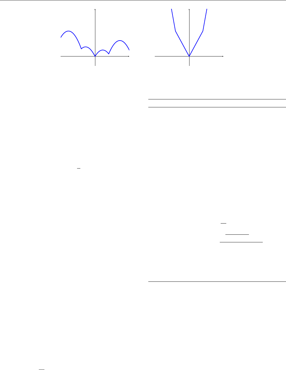
Figure 1: Example of a weakly convex function. The left ﬁgure is the original weakly convex function. By adding

an appropriate quadratic to the weakly convex function (left), we get the convex function on the right.

exploit the problem structure (ﬁnite-sum, composite)

in the convex case, and beneﬁt from this feature when

dealing with a new problem with unknown convexity;

remarkably,

does not need to have any convergence

guarantee for nonconvex problems to be used in 4WD-

Catalyst, which is the main originality of our work.

Two-step subproblems.

In each iteration, 4WD-

Catalyst forms subproblems of the form

min

(x; y) := f(x) +

kx − yk

. (P)

We call

the prox-center and any minimizer of the

subproblem a proximal point. The perturbed function

(

;

) satisﬁes the important property:

(

;

) is

(

κ − ρ

)-strongly convex for any

κ > ρ

. The addition of

the quadratic to

makes the subproblem more “con-

vex”. That is, when

is nonconvex, a large enough

yields convex subproblems; even when

is convex, the

quadratic perturbation improves conditioning.

We now describe the

’th iteration of Algorithm 1. To

this end, suppose we have available iterates

k−1

and

k−1

. At the center of our Algorithm 1 are two main

sequences of iterates (

¯x

)

and (

˜x

)

, obtained from

approximately solving two subproblems of the form

1. Proximal point step.

We ﬁrst perform an inexact

proximal point step with prox-center x

k−1

¯x

≈ argmin

(x; x

k−1

) [Proximal-point step] (2)

2. Accelerated proximal point step.

Then we

build the next prox-center y

as the combination

= α

k−1

+ (1 − α

k−1

. (3)

Next we use

as a prox-center and update the next

extrapolation term:

˜x

≈ argmin

(x; y

) [Acc. prox.-point step] (4)

= x

k−1

(˜x

− x

k−1

) [Extrapolation] (5)

where

k+1

∈

1) is a sequence of coeﬃcients sat-

isfying

(1 − α

k+1

)/α

k+1

= 1/α

. Essentially, the se-

quences (

)

(

)

(

)

are built upon the extrapo-

lation principles of [26].

Algorithm 1 4WD-Catalyst

input

Fix a point

∈ dom f

, real numbers

, κ

cvx

0 and T, S > 0, and an opt. method M.

initialization: α

= 1, v

= x

repeat for k = 1, 2, . . .

1. Compute

(¯x

, κ

) = Auto-adapt (x

k−1

, κ

k−1

, T ).

Compute

k−1

+ (1

− α

)

k−1

and

apply S log(k + 1) iterations of M to ﬁnd

˜x

≈ argmin

x∈R

cvx

(x, y

). (6)

3. Update v

and α

k+1

= x

k−1

(˜x

− x

k−1

)

and α

k+1

+ 4α

− α

Choose

to be any point satisfying

(

) =

min{f(¯x

), f (˜x

)}.

until the stopping criterion dist



0, ∂f (¯x

)



< ε

Picking the best.

At the end of iteration

, we

have two iterates, resp.

¯x

and

˜x

. Following [

we simply choose the best of the two in terms of their

objective values, that is we choose

such that

(

)

≤

min {f (¯x

), f (˜x

)}.

The proposed scheme blends the two steps in a syner-

gistic way, allowing us to recover the near-optimal rates

of convergence in both worlds: convex and nonconvex.

Intuitively, when

¯x

is chosen, it means that Nesterov’s

extrapolation step “fails” to accelerate convergence.

We present now our strategy to set the parameters of

4WD-Catalyst in order to a) automatically adapt to

the unknown weak convexity constant

; b) enjoy near-

optimal rates in both convex and nonconvex settings.

Courtney Paquette, Hongzhou Lin, Dmitriy Drusvyatskiy, Julien Mairal, Zaid Harchaoui

Algorithm 2 Auto-adapt (x, κ, T )

input x ∈ R

, method M, κ > 0, num. iterations T .

Repeat

Run

iterations of

initializing from

, or

prox

ηψ

(

x − η∇f

(

;

)) with

(

) for composite objectives

with

L-smooth function f

, to obtain

≈ argmin

z∈R

(z; x).

If f

; x) ≤ f

(x; x)

and dist(0, ∂f

; x)) ≤ κ kz

− xk,

then go to output.

else repeat with κ → 2κ.

output (z

, κ).

4 Parameter Choices and Adaptation

When

is large enough, the subproblems become

strongly convex; thus globally solvable. Henceforth,

we will assume that

satisﬁes the following natural

linear convergence assumption.

Linear convergence of M for strongly-convex

problems.

We assume that for any

κ > ρ

, there

exist

≥

0 and

in (0

1) so that the following hold:

For any prox-center

, deﬁne

∗

(

) =

min

(

z, y

). For any initial point

, the

iterates

}

t≥1

generated by

on the problem

min

(z; y) satisfy

dist

(0, ∂f

; y)) ≤ A

(1−τ

)



; y)−f

∗

(y)



(7)

The rates

and constants

are increasing in

When the function is strongly convex, the ﬁrst condition

is equivalent to the error

(

;

)

− f

∗

(

) decreasing

geometrically to zero (convergence in sub-gradient norm

and function values are equivalent in this case). If

the method is randomized, we allow

(7)

to hold in

expectation; see Sec. 5.1 in [

]. All algorithms of

interest, (e.g., gradient descent, SVRG, SAGA) satisfy

these properties.

Adaptation to weak convexity and choice of T .

Recall that we add a quadratic to

to make each sub-

problem convex. Thus, we should set

κ > ρ

, if

were

known. On the other other hand, we do not want

too

large, as that may slow down the overall algorithm. In

any case, it is diﬃcult to have an accurate estimate of

for machine learning problems such as neural networks.

Thus, we propose a procedure described in Algorithm 2

to automatically adapt to ρ.

The idea is to ﬁx in advance a number of iterations

let

run on the subproblem for

iterations, output

the point

, and check if a suﬃcient decrease occurs.

We show that if we set

(

−1

), where

hides

logarithmic dependencies in

and

, where

is the

Lipschitz constant of the smooth part of

; then, if

the subproblem were convex, the following conditions

would be guaranteed:

1. Descent condition: f

; x) ≤ f

(x; x);

2. Adaptive stationary condition:

dist



0, ∂f

; x)



≤ κ kz

− xk.

Thus, if either condition is not satisﬁed, then the sub-

problem is deemed not convex and we double

and

repeat. The procedure yields an estimate of

in a

logarithmic number of increases; see [28][Lemma D.3].

The descent condition is a sanity check, which ensures

the iterates generated by the algorithm always decrease

the function value. Without it, the stationarity con-

dition alone is insuﬃcient because of the existence of

local maxima in nonconvex problems.

The adaptive stationarity property controls the in-

exactness of the subproblem in terms of subgradi-

ent norm. In a nonconvex setting, the subgradient

norm is convenient, since we cannot access

(

, x

)

−

∗

(

). Furthermore, unlike the stationary condition

dist



, ∂f

(

;

)



< ε

, where an accuracy

is pre-

deﬁned, the adaptive stationarity condition depends

on the iterate

. This turns out to be essential in

deriving the global complexity. Sec. 4 in [

] contains

more details.

Relative stationarity and predeﬁning S.

One of

the main diﬀerences of our approach with the Catalyst

algorithm of [

] is to use a pre-deﬁned number of

iterations,

and

, for solving the subproblems. We

introduce

cvx

, a

dependent smoothing parameter,

and set it in the same way as the smoothing parameter

in [

]. The automatic acceleration of our algorithm

when the problem is convex is due to extrapolation

steps in Step 2-3 of Algo. 1. We show that if we set



−1

cvx



, where

hides logarithmic dependencies

, and

cvx

, then we can be sure that in the

convex setting we have

dist



0, ∂f

cvx

(˜x

; y

)



cvx

k + 1

k˜x

− y

k. (8)

This relative stationarity of

˜x

, including the choice

cvx

, shall be crucial to guarantee that the scheme

accelerates in the convex setting. An additional

1 factor appears compared to the previous adaptive

stationary condition because we need higher accuracy

for solving the subproblem to achieve the accelerated

rate in 1

√

. Therefore, an extra

log

(

+ 1) factor of

iterations is needed; see Sec. 4 and Sec. 5 in [28].

We shall see, in Sec. 6, that our strategy consisting in

predeﬁning T and S works quite well in practice.

Catalyst for Gradient-based Nonconvex Optimization

The worst-case theoretical bounds we derive are con-

servative; we observe in our experiments that one may

choose

and

signiﬁcantly smaller than the theory

suggests and still retain the stopping criteria.

5 Global Convergence and

Applications to Existing Algorithms

After presenting the main mechanisms of our algoritm,

we now present its worst-case complexity, which takes

into account the cost of approximately solving the

subproblems (2) and (4).

Theorem 5.1

(Global complexity bounds for 4WD–

Catalyst)

Choose

(

−1

) and

(

−1

cvx

) (see

Theorem 5.6 in [28]). Then the following are true.

Algorithm 1 generates a point

satisfying

dist



0, ∂f (x)



≤ ε after at most





−1

+ τ

−1

cvx



L(f(x

) − f

∗

)



iterations of the method M.

is convex, Algorithm 1 generates a point

satisfying dist



0, ∂f (x)



≤ ε after at most



−1

+ τ

−1

cvx



1/3



cvx

∗

− x



1/3

2/3

iterations of the method M.

is convex, Algorithm 1 generates a point

satisfying f (x) − f

∗

≤ ε after at most



−1

+ τ

−1

cvx



cvx

∗

− x

√

iterations of the method M.

Here

hides universal constants and logarith-

mic dependencies in

cvx

, and

∗

− x

is a ﬁrst order method, the convergence guarantee

in the convex setting is near-optimal, up to logarithmic

factors, when compared to

√

) [

]. In the

nonconvex setting, our approach matches, up to loga-

rithmic factors, the best known rate for this class of

functions, namely

/ε

) [

]. Moreover, our rates

dependence on the dimension and Lipschitz constant

equals, up to log factors, the best known dependencies

in both the convex and nonconvex setting. These loga-

rithmic factors may be the price we pay for having a

generic algorithm.

Choice of κ

cvx

The parameter

cvx

drives the con-

vergence rate of 4WD-Catalyst in the convex setting.

To determine

cvx

, we compute the global complexity

of our scheme as if

= 0, hence using the same reason-

ing as [

]. The rule consists in maximizing the ratio

√

. Then, the choice of

is independent of

;

it is an initial lower estimate for the weak convexity

constant

. We provide a detailed derivation of all

the variables for each of the considered algorithms in

Section 6 of [28].

5.1 Applications

We now compare the guarantees obtained before and

after applying 4WD-Catalyst to some speciﬁc optimiza-

tion methods

: full gradient, SAGA, and SVRG (see

[

] for randomized coordinate descent). In the convex

setting, the accuracy is stated in terms of optimization

error,

(

)

− f

≤ ε

and in the nonconvex setting, in

terms of stationarity condition dist(0, ∂f(x)) < ε.

Full gradient method.

First, we consider the sim-

plest case of applying our method to the full gradi-

ent method (FG). Here, the optimal choice for

cvx

. In the convex setting, we get the accelerated rate

(

L/ε log

/ε

)) which is consistent with Nesterov’s

accelerated variant (AFG) up to log factors. In the

nonconvex case, our approach achieves no worse rate

than

(

nL/ε

log

/ε

)), which is consistent with the

standard gradient descent up to log factors. Under

stronger assumptions, namely

-smoothness of the

objective, the accelerated algorithm in [

] can achieve

the same rate as (AFG) in the convex setting and

(

−7/4

log

/ε

)) in the nonconvex setting. Their ap-

proach, however, does not extend to composite setting

nor to stochastic methods. The marginal loss may be

the price for considering a larger class of functions.

Randomized incremental gradient.

We now con-

sider randomized incremental gradient methods such

as SAGA [

] and (prox) SVRG [

]. Here, the optimal

choice for

cvx

(

L/n

). Under the convex setting,

we achieve an accelerated rate of

(

√

L/ε log

/ε

)).

Direct applications of SVRG and SAGA have no con-

vergence guarantees in the nonconvex setting, but with

our approach, the resulting algorithm matches the guar-

antees of FG up to log factors, see Table 1 for details.

6 Experiments

We investigate the performance of 4WD-Catalyst on

two standard nonconvex problems in machine learning,

namely on sparse matrix factorization and on training

a simple two-layer neural network.

Comparison with linearly convergent methods.

We report experimental results of 4WD-Catalyst when

applied to the incremental algorithms SVRG [

] and

SAGA [9], and consider the following variants:

Courtney Paquette, Hongzhou Lin, Dmitriy Drusvyatskiy, Julien Mairal, Zaid Harchaoui

•

ncvx-SVRG/SAGA [

] with its theoretical step-

size η = 1/Ln

2/3

•

a minibatch variant of ncvx-SVRG/SAGA [

]

with batch size b = n

2/3

and stepsize η = 1/L.

•

SVRG/SAGA with large stepsize

= 1

. This is

a variant of SVRG/SAGA, whose stepsize is not jus-

tiﬁed by theory for nonconvex problems, but which

performs well in practice.

•

4WD-Catalyst SVRG/SAGA with its theoretical

stepsize η = 1/2L.

The algorithm SVRG (resp. SAGA) was originally

designed for minimizing convex objectives. The non-

convex version was developed in [

], using a signif-

icantly smaller stepsize

= 1

/Ln

2/3

. Following [

we also include in the comparison a heuristic variant

that uses a large stepsize

= 1

, where no theoretical

guarantee is available for nonconvex objectives. 4WD-

Catalyst SVRG and 4WD-Catalyst SAGA use a similar

stepsize, but the Catalyst mechanism makes this choice

theoretically grounded.

Comparison with popular stochastic algorithms.

We also include as baselines three popular stochastic

algorithms: stochastic gradient descent (SGD), Ada-

Grad [11], and Adam [17].

• SGD with constant stepsize.

• AdaGrad [11] with stepsize η = 0.1 or 0.01.

•

Adam [

] with stepsize

= 0

01 or 0

001,

= 0

and β

= 0.999.

The stepsize (learning rate) of these algorithms are

manually tuned to output the best performance. Note

that none of them, SGD, AdaGrad [

] or Adam [

]

enjoys linear convergence when the problem is strongly

convex. Therefore, we do not apply 4WD-Catalyst to

these algorithms. SGD is used in both experiments,

whereas AdaGrad and Adam are used only on the

neural network experiments since it is unclear how to

apply them to a nonsmooth objective.

Parameter settings.

We start from an initial esti-

mate of the Lipschitz constant

and use the theoret-

ically recommended parameters

cvx

= 2

L/n

4WD-Catalyst. We set the number of inner iterations

in all experiments which means making at

most one pass over the data to solve each sub-problem.

Moreover, the

log

(

) dependency dictated by the the-

ory is dropped while solving the subproblem in (6).

These choices turn out to be justiﬁed a posteriori, as

both SVRG and SAGA have a much better convergence

rate in practice than the theoretical rate derived from

a worst-case analysis. Indeed, in all experiments, one

pass over the data to solve each sub-problem was found

to be enough to guarantee suﬃcient descent. We focus

in the main text on the results for SVRG and relegate

results for SAGA and details about experiments to

Section 7 of [28].

Sparse matrix factorization a.k.a. dictionary

learning.

Dictionary learning consists of represent-

ing a dataset

= [

, ··· , x

]

∈ R

m×n

as a product

X ≈ DA

, where

m×p

is called a dictionary, and

p×n

is a sparse matrix. The classical nonconvex

formulation [see

] can be reformulated as the equiv-

alent ﬁnite-sum problem

min

D∈C

i=1

(

) with

(D) := min

α∈R

− Dαk

+ ψ(α). (9)

is a sparsity-inducing regularization and

is chosen

as the set of matrices whose columns are in the

-ball;

see Sec. 7 in [

]. We consider elastic-net regularization

(

) =

kαk

λkαk

of [

], which has a sparsity-

inducing eﬀect, and report the corresponding results in

Figure 2. We learn a dictionary in

m×p

with

= 256

elements on a set of whitened normalized image patches

of size

= 8

8. Parameters are set to be as in [

]—

that is, a small value

e−

5, and

25, leading to

sparse matrices

(on average

≈

4 non-zero coeﬃcients

per column of A).

Neural networks.

We consider simple binary classi-

ﬁcation problems for learning neural networks. Assume

that we are given a training set

, b

}

i=1

, where the

variables

{−

}

represent class labels, and

are feature vectors. The estimator of a la-

bel class is now given by a two-layer neural network

sign

(

)), where

p×d

represents

the weights of a hidden layer with

neurons,

carries the weight of the network’s second layer, and

(

) =

log

(1 +

) is a non-linear function, applied

point-wise to its arguments. We use the logistic loss to

ﬁt the estimators to the true labels and report experi-

mental results on the two datasets alpha and covtype.

The weights of the network are randomly initialized

and we ﬁx the number of hidden neurons to d = 100.

Computational cost.

For SGD, AdaGrad, Adam,

and all the ncvx-SVRG variants, one iteration corre-

sponds to one pass over the data in the plots. For 4WD-

Catalyst-SVRG, it solves two sub-problems per itera-

tion, which doubles the cost per iteration comparing

to the other algorithms. It is worth remarking that

every time acceleration occurs in our experiments,

˜x

is almost always preferred to

¯x

in step 4 of 4WD-

Catalyst, suggesting that half of the computations may

be reduced when running 4WD-Catalyst-SVRG.

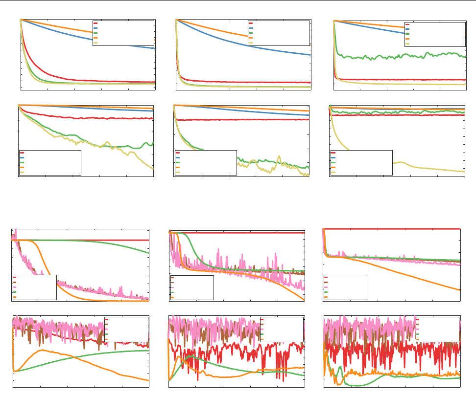
Experimental conclusions.

In the matrix factor-

ization experiments in Fig. 2, 4WD-Catalyst-SVRG

was always competitive, with a similar performance

to the heuristic SVRG-

= 1

in two cases out of

three, while being signiﬁcantly better as soon as the

Catalyst for Gradient-based Nonconvex Optimization

0 20 40 60 80 100

Number of iterations

0.36

0.38

0.4

0.42

0.44

0.46

0.48

0.5

0.52

0.54

0.56

Function value

Matrix factorization, n=1000

sgd

ncvx svrg th. η

svrg η = 1/L

ncvx svrg minibatch th. η

4wd-catalyst svrg

0 20 40 60 80 100

Number of iterations

0.48

0.49

0.5

0.51

0.52

0.53

0.54

0.55

0.56

0.57

0.58

Function value

Matrix factorization, n=10000

sgd

ncvx svrg th. η

svrg η = 1/L

ncvx svrg minibatch th. η

4wd-catalyst svrg

0 20 40 60 80 100

Number of iterations

0.46

0.465

0.47

0.475

0.48

0.485

0.49

0.495

0.5

0.505

0.51

Function value

Matrix factorization, n=100000

sgd

ncvx svrg th. η

svrg η = 1/L

ncvx svrg minibatch th. η

4wd-catalyst svrg

0 20 40 60 80 100

Number of iterations

-5

-4.5

-4

-3.5

-3

-2.5

-2

Log of Subgradient Norm

Matrix factorization, n=1000

sgd

ncvx svrg th. η

svrg η = 1/L

ncvx svrg minibatch th. η

4wd-catalyst svrg

0 20 40 60 80 100

Number of iterations

-4.5

-4

-3.5

-3

-2.5

-2

Log of Subgradient Norm

Matrix factorization, n=10000

sgd

ncvx svrg th. η

svrg η = 1/L

ncvx svrg minibatch th. η

4wd-catalyst svrg

0 20 40 60 80 100

Number of iterations

-4.2

-4

-3.8

-3.6

-3.4

-3.2

-3

-2.8

-2.6

Log of Subgradient Norm

Matrix factorization, n=100000

sgd

ncvx svrg th. η

svrg η = 1/L

ncvx svrg minibatch th. η

4wd-catalyst svrg

Figure 2: Dictionary learning experiments. We plot the function value (top) and the subgradient norm (bottom).

From left to right, we vary the size of the dataset from n = 1 000 to n = 100 000

0 50 100 150 200 250

Number of iterations

0.1

0.2

0.3

0.4

0.5

0.6

0.7

0.8

Function value

Neural network, dataset=alpha, n=1000

sgd

adagrad

adam

svrg η = 1/L

4wd-catalyst svrg

0 50 100 150 200 250

Number of iterations

0.2

0.25

0.3

0.35

0.4

0.45

0.5

0.55

0.6

0.65

0.7

Function value

Neural network, dataset=alpha, n=10000

sgd

adagrad

adam

svrg η = 1/L

4wd-catalyst svrg

0 50 100 150 200 250

Number of iterations

0.1

0.2

0.3

0.4

0.5

0.6

Function value

Neural network, dataset=alpha, n=100000

sgd

adagrad

adam

svrg η = 1/L

4wd-catalyst svrg

0 50 100 150 200 250

Number of iterations

-5

-4.5

-4

-3.5

-3

-2.5

-2

-1.5

-1

-0.5

Log of Subgradient Norm

Neural network, dataset=alpha, n=1000

sgd

adagrad

adam

svrg η = 1/L

4wd-catalyst svrg

0 50 100 150 200 250

Number of iterations

-4.5

-4

-3.5

-3

-2.5

-2

-1.5

-1

-0.5

Log of Subgradient Norm

Neural network, dataset=alpha, n=10000

sgd

adagrad

adam

svrg η = 1/L

4wd-catalyst svrg

0 50 100 150 200 250

Number of iterations

-4.5

-4

-3.5

-3

-2.5

-2

-1.5

-1

-0.5

Log of Subgradient Norm

Neural network, dataset=alpha, n=100000

sgd

adagrad

adam

svrg η = 1/L

4wd-catalyst svrg

Figure 3: Neural network experiments. Same experimental setup as in Fig. 2. From left to right, we vary the size

of the dataset’s subset from n = 1 000 to n = 100 000.

amount of data n was large enough. As expected, the

variants of SVRG with theoretical stepsizes have slow

convergence, but exhibit a stable behavior compared

to SVRG-

= 1

. This conﬁrms the ability of 4WD-

Catalyst-SVRG to adapt to nonconvex terrains. Simi-

lar conclusions hold when applying 4WD-Catalyst to

SAGA; see Sec. 7 in [28].

In the neural network experiments, we observe

that 4WD-Catalyst-SVRG converges much faster over-

all in terms of objective values than other algorithms.

Yet Adam and AdaGrad often perform well during the

ﬁrst iterations, they oscillate a lot, which is a behavior

commonly observed. In contrast, 4WD-Catalyst-SVRG

always decreases and keeps decreasing while other algo-

rithms tend to stabilize, hence achieving signiﬁcantly

lower objective values.

More interestingly, as the algorithm proceeds, the sub-

gradient norm may increase at some point and then

decrease, while the function value keeps decreasing.

This suggests that the extrapolation step, or the Auto-

adapt procedure, is helpful to escape bad stationary

points, e.g., saddle-points. We leave the study of this

particular phenomenon as a potential direction for fu-

ture work.

Acknowledgements

The authors would like to thank J. Duchi for fruit-

ful discussions. CP was partially supported by the

LMB program of CIFAR. HL and JM were supported

by ERC grant SOLARIS (# 714381) and ANR grant

MACARON (ANR-14-CE23-0003-01). DD was sup-

ported by AFOSR YIP FA9550-15-1-0237, NSF DMS

1651851, and CCF 1740551 awards. ZH was supported

by NSF Grant CCF-1740551, the “Learning in Ma-

chines and Brains” program of CIFAR, and a Criteo

Faculty Research Award. This work was performed

while HL was at Inria.

Courtney Paquette, Hongzhou Lin, Dmitriy Drusvyatskiy, Julien Mairal, Zaid Harchaoui

References

[1]

Z. Allen-Zhu. Natasha: Faster non-convex stochas-

tic optimization via strongly non-convex parame-

ter. In International conference on machine learn-

ing (ICML), 2017.

[2]

Z. Allen-Zhu and E. Hazan. Variance reduction for

faster non-convex optimization. In International

conference on machine learning (ICML), 2016.

[3]

J. M. Borwein and A. S. Lewis. Convex analysis

and nonlinear optimization: theory and examples.

Springer Verlag, 2006.

[4]

Y. Carmon, J. C. Duchi, O. Hinder, and A. Sidford.

Accelerated methods for non-convex optimization.

preprint arXiv:1611.00756, 2016.

[5]

Y. Carmon, J. C. Duchi, O. Hinder, and A. Sid-

ford. Lower bounds for ﬁnding stationary points

I. preprint arXiv:1710.11606, 2017.

[6]

Y. Carmon, O. Hinder, J. C. Duchi, and A. Sid-

ford. “convex until proven guilty”: Dimension-free

acceleration of gradient descent on non-convex

functions. In International conference on machine

learning (ICML), 2017.

[7]

C. Cartis, N. I. M. Gould, and P. L. Toint. On

the complexity of steepest descent, newton’s and

regularized newton’s methods for nonconvex un-

constrained optimization problems. SIAM Journal

on Optimization, 20(6):2833–2852, 2010.

[8]

C. Cartis, N.I.M. Gould, and P. L. Toint. On the

complexity of ﬁnding ﬁrst-order critical points in

constrained nonlinear optimization. Mathematical

Programming, Series A, 144:93–106, 2014.

[9]

A. J. Defazio, F. Bach, and S. Lacoste-Julien.

SAGA: A fast incremental gradient method with

support for non-strongly convex composite objec-

tives. In Advances in Neural Information Process-

ing Systems (NIPS), 2014.

[10]

D. Drusvyatskiy and C. Paquette. Eﬃciency of

minimizing compositions of convex functions and

smooth maps. preprint arXiv:1605.00125, 2016.

[11]

J. C. Duchi, E. Hazan, and Y. Singer. Adap-

tive subgradient methods for online learning and

stochastic optimization. Journal of Machine

Learning Research (JMLR), 12:2121–2159, 2011.

[12]

S. Ghadimi and G. Lan. Accelerated gradient

methods for nonconvex nonlinear and stochastic

programming. Mathematical Programming, 156(1-

2, Ser. A):59–99, 2016.

[13]

S. Ghadimi, G. Lan, and H. Zhang. Generalized

uniformly optimal methods for nonlinear program-

ming. preprint arXiv:1508.07384, 2015.

[14]

T. Hastie, R. Tibshirani, and M. Wainwright. Sta-

tistical learning with sparsity: the Lasso and gen-

eralizations. CRC Press, 2015.

[15]

C. Jin, P. Netrapalli, and M. I. Jordan. Accelerated

gradient descent escapes saddle points faster than

gradient descent. preprint arXiv:1711.10456, 2017.

[16]

R. Johnson and T. Zhang. Accelerating stochastic

gradient descent using predictive variance reduc-

tion. In Advances in Neural Information Process-

ing Systems (NIPS), 2013.

[17]

Diederik P Kingma and Jimmy Ba. Adam: A

method for stochastic optimization. International

Conference on Learning Representations (ICLR),

2015.

[18]

G. Lan and Y. Zhou. An optimal randomized

incremental gradient method. Mathematical Pro-

gramming, Series A, pages 1–38, 2017.

[19]

L. Lei and M. I. Jordan. Less than a single

pass: stochastically controlled stochastic gradient

method. In Conference on Artiﬁcial Intelligence

and Statistics (AISTATS), 2017.

[20]

L. Lei, C. Ju, J. Chen, and M. I. Jordan. Non-

convex ﬁnite-sum optimization via SCSG meth-

ods. In Advances in Neural Information Processing

Systems (NIPS), 2017.

[21]

H. Li and Z. Lin. Accelerated proximal gradient

methods for nonconvex programming. In Advances

in Neural Information Processing Systems (NIPS).

2015.

[22]

H. Lin, J. Mairal, and Z. Harchaoui. A universal

catalyst for ﬁrst-order optimization. In Advances

in Neural Information Processing Systems (NIPS),

2015.

[23]

J. Mairal. Incremental majorization-minimization

optimization with application to large-scale ma-

chine learning. SIAM Journal on Optimization,

25(2):829–855, 2015.

[24]

J. Mairal, F. Bach, and J. Ponce. Sparse modeling

for image and vision processing. Foundations and

Trends in Computer Graphics and Vision, 8(2-

3):85–283, 2014.

[25]

Y. Nesterov. A method of solving a convex pro-

gramming problem with convergence rate

(1/

Soviet Mathematics Doklady, 27(2):372–376, 1983.

[26]

Y. Nesterov. Introductory lectures on convex opti-

mization: a basic course. Springer, 2004.

[27]

M. O’Neill and S. J. Wright. Behavior of accel-

erated gradient methods near critical points of

nonconvex problems. preprint arXiv:1706.07993,

2017.

Catalyst for Gradient-based Nonconvex Optimization

[28]

C. Paquette, H. Lin, D. Drusvyatskiy, J. Mairal,

and Z. Harchaoui. Catalyst acceleration for

gradient-based non-convex optimization. preprint

arXiv:1703.10993, 2017.

[29]

S. J. Reddi, A. Hefny, S. Sra, B. Poczos, and

A. Smola. Stochastic variance reduction for non-

convex optimization. In International conference

on machine learning (ICML), 2016.

[30]

S. J. Reddi, S. Sra, B. Poczos, and A. J. Smola.

Proximal stochastic methods for nonsmooth non-

convex ﬁnite-sum optimization. In Advances in

Neural Information Processing Systems (NIPS),

2016.

[31]

R. T. Rockafellar and R. J.-B. Wets. Variational

analysis, volume 317 of Grundlehren der Mathema-

tischen Wissenschaften [Fundamental Principles

of Mathematical Sciences]. Springer-Verlag, Berlin,

1998.

[32]

M. Schmidt, N. Le Roux, and F. Bach. Minimizing

ﬁnite sums with the stochastic average gradient.

Mathematical Programming, 162(1):83–112, 2017.

[33]

B. E. Woodworth and N. Srebro. Tight complexity

bounds for optimizing composite objectives. In Ad-

vances in Neural Information Processing Systems

(NIPS). 2016.

[34]

L. Xiao and T. Zhang. A proximal stochastic gra-

dient method with progressive variance reduction.

SIAM Journal on Optimization, 24(4):2057–2075,

2014.

[35]

H. Zou and T. Hastie. Regularization and variable

selection via the elastic net. Journal of the Royal

Statistical Society: Series B (Statistical Methodol-

ogy), 67(2):301–320, 2005.