Catalyst Acceleration for First-order Convex Optimization: from

Journal of Machine Learning Research 18 (2018) 1-54 Submitted 12/17; Revised 12/17; Published 4/18

Catalyst Acceleration for First-order Convex Optimization:

from Theory to Practice

Hongzhou Lin [email protected]

Massachusetts Institute of Technology

Computer Science and Artiﬁcial Intelligence Laboratory

Cambridge, MA 02139, USA

Julien Mairal [email protected]

Univ. Grenoble Alpes, Inria, CNRS, Grenoble INP

∗

, LJK,

Grenoble, 38000, France

Zaid Harchaoui [email protected]

University of Washington

Department of Statistics

Seattle, WA 98195, USA

Editor: L´eon Bottou

Abstract

We introduce a generic scheme for accelerating gradient-based optimization methods in

the sense of Nesterov. The approach, called Catalyst, builds upon the inexact acceler-

ated proximal point algorithm for minimizing a convex objective function, and consists of

approximately solving a sequence of well-chosen auxiliary problems, leading to faster con-

vergence. One of the keys to achieve acceleration in theory and in practice is to solve these

sub-problems with appropriate accuracy by using the right stopping criterion and the right

warm-start strategy. We give practical guidelines to use Catalyst and present a compre-

hensive analysis of its global complexity. We show that Catalyst applies to a large class of

algorithms, including gradient descent, block coordinate descent, incremental algorithms

such as SAG, SAGA, SDCA, SVRG, MISO/Finito, and their proximal variants. For all of

these methods, we establish faster rates using the Catalyst acceleration, for strongly convex

and non-strongly convex objectives. We conclude with extensive experiments showing that

acceleration is useful in practice, especially for ill-conditioned problems.

Keywords: convex optimization, ﬁrst-order methods, large-scale machine learning

1. Introduction

A large number of machine learning and signal processing problems are formulated as the

minimization of a convex objective function:

min

x∈R

f(x) , f

(x) + ψ(x)

, (1)

where f

is convex and L-smooth, and ψ is convex but may not be diﬀerentiable. We call

a function L-smooth when it is diﬀerentiable and its gradient is L-Lipschitz continuous.

∗. Institute of Engineering Univ. Grenoble Alpes

2018 Hongzhou Lin, Julien Mairal and Zaid Harchaoui.

License: CC-BY 4.0, see https://creativecommons.org/licenses/by/4.0/. Attribution requirements are provided

at http://jmlr.org/papers/v18/17-748.html.

Lin, Mairal and Harchaoui

In statistics or machine learning, the variable x may represent model parameters, and

the role of f

is to ensure that the estimated parameters ﬁt some observed data. Speciﬁcally,

is often a large sum of functions and (1) is a regularized empirical risk which writes as

min

x∈R

(

f(x) ,

i=1

(x) + ψ(x)

)

. (2)

Each term f

(x) measures the ﬁt between x and a data point indexed by i, whereas the

function ψ acts as a regularizer; it is typically chosen to be the squared `

-norm, which

is smooth, or to be a non-diﬀerentiable penalty such as the `

-norm or another sparsity-

inducing norm (Bach et al., 2012).

We present a uniﬁed framework allowing one to accelerate gradient-based or ﬁrst-order

methods, with a particular focus on problems involving large sums of functions. By “ac-

celerating”, we mean generalizing a mechanism invented by Nesterov (1983) that improves

the convergence rate of the gradient descent algorithm. When ψ = 0, gradient descent

steps produce iterates (x

)

k≥0

such that f(x

) − f

∗

≤ ε in O(1/ε) iterations, where f

∗

denotes the minimum value of f. Furthermore, when the objective f is µ-strongly convex,

the previous iteration-complexity becomes O((L/µ) log(1/ε)), which is proportional to the

condition number L/µ. However, these rates were shown to be suboptimal for the class

of ﬁrst-order methods, and a simple strategy of taking the gradient step at a well-chosen

point diﬀerent from x

yields the optimal complexity—O(1/

√

ε) for the convex case and

L/µ log(1/ε)) for the µ-strongly convex one (Nesterov, 1983). Later, this acceleration

technique was extended to deal with non-diﬀerentiable penalties ψ for which the proximal

operator deﬁned below is easy to compute (Beck and Teboulle, 2009; Nesterov, 2013).

prox

(x) , arg min

z∈R



ψ(z) +

kx − zk



, (3)

where k.k denotes the Euclidean norm.

For machine learning problems involving a large sum of n functions, a recent eﬀort has

been devoted to developing fast incremental algorithms such as SAG (Schmidt et al., 2017),

SAGA (Defazio et al., 2014a), SDCA (Shalev-Shwartz and Zhang, 2012), SVRG (Johnson

and Zhang, 2013; Xiao and Zhang, 2014), or MISO/Finito (Mairal, 2015; Defazio et al.,

2014b), which can exploit the particular structure (2). Unlike full gradient approaches,

which require computing and averaging n gradients (1/n)

i=1

∇f

(x) at every iteration,

incremental techniques have a cost per-iteration that is independent of n. The price to pay is

the need to store a moderate amount of information regarding past iterates, but the beneﬁts

may be signiﬁcant in terms of computational complexity. In order to achieve an ε-accurate

solution for a µ-strongly convex objective, the number of gradient evaluations required by

the methods mentioned above is bounded by O



n +



log(

)



, where

L is either the

maximum Lipschitz constant across the gradients ∇f

, or the average value, depending

on the algorithm variant considered. Unless there is a big mismatch between

L and L

(global Lipschitz constant for the sum of gradients), incremental approaches signiﬁcantly

outperform the full gradient method, whose complexity in terms of gradient evaluations is

bounded by O



log(

)



Catalyst for First-order Convex Optimization

Yet, these incremental approaches do not use Nesterov’s extrapolation steps and whether

or not they could be accelerated was an important open question when these methods were

introduced. It was indeed only known to be the case for SDCA (Shalev-Shwartz and Zhang,

2016) for strongly convex objectives. Later, other accelerated incremental algorithms were

proposed such as Katyusha (Allen-Zhu, 2017), or the method of Lan and Zhou (2017).

We give here a positive answer to this open question. By analogy with substances that

increase chemical reaction rates, we call our approach “Catalyst”. Given an optimization

method M as input, Catalyst outputs an accelerated version of it, eventually the same algo-

rithm if the method M is already optimal. The sole requirement on the method in order to

achieve acceleration is that it should have linear convergence rate for strongly convex prob-

lems. This is the case for full gradient methods (Beck and Teboulle, 2009; Nesterov, 2013)

and block coordinate descent methods (Nesterov, 2012; Richt´arik and Tak´aˇc, 2014), which

already have well-known accelerated variants. More importantly, it also applies to the pre-

viou incremental methods, whose complexity is then bounded by



n +

L/µ



log(

)



after Catalyst acceleration, where

O hides some logarithmic dependencies on the condition

number

L/µ. This improves upon the non-accelerated variants, when the condition num-

ber is larger than n. Besides, acceleration occurs regardless of the strong convexity of the

objective—that is, even if µ = 0—which brings us to our second achievement.

Some approaches such as MISO, SDCA, or SVRG are only deﬁned for strongly convex

objectives. A classical trick to apply them to general convex functions is to add a small

regularization term εkxk

in the objective (Shalev-Shwartz and Zhang, 2012). The drawback

of this strategy is that it requires choosing in advance the parameter ε, which is related

to the target accuracy. The approach we present here provides a direct support for non-

strongly convex objectives, thus removing the need of selecting ε beforehand. Moreover, we

can immediately establish a faster rate for the resulting algorithm. Finally, some methods

such as MISO are numerically unstable when they are applied to strongly convex objective

functions with small strong convexity constant. By deﬁning better conditioned auxiliary

subproblems, Catalyst also provides better numerical stability to these methods.

A short version of this paper has been published at the NIPS conference in 2015 (Lin

et al., 2015a); in addition to simpler convergence proofs and more extensive numerical evalu-

ation, we extend the conference paper with a new Moreau-Yosida smoothing interpretation

with signiﬁcant theoretical and practical consequences as well as new practical stopping

criteria and warm-start strategies.

The paper is structured as follows. We complete this introductory section with some

related work in Section 1.1, and give a short description of the two-loop Catalyst algorithm

in Section 1.2. Then, Section 2 introduces the Moreau-Yosida smoothing and its inexact

variant. In Section 3, we introduce formally the main algorithm, and its convergence analysis

is presented in Section 4. Section 5 is devoted to numerical experiments and Section 6

concludes the paper.

1.1 Related Work

Catalyst can be interpreted as a variant of the proximal point algorithm (Rockafellar, 1976;

G¨uler, 1991), which is a central concept in convex optimization, underlying augmented

Lagrangian approaches, and composite minimization schemes (Bertsekas, 2015; Parikh and

Lin, Mairal and Harchaoui

Boyd, 2014). The proximal point algorithm consists of solving (1) by minimizing a sequence

of auxiliary problems involving a quadratic regularization term. In general, these auxiliary

problems cannot be solved with perfect accuracy, and several notions of inexactness were

proposed by G¨uler (1992); He and Yuan (2012) and Salzo and Villa (2012). The Cata-

lyst approach hinges upon (i) an acceleration technique for the proximal point algorithm

originally introduced in the pioneer work of G¨uler (1992); (ii) a more practical inexact-

ness criterion than those proposed in the past.

As a result, we are able to control the

rate of convergence for approximately solving the auxiliary problems with an optimization

method M. In turn, we are also able to obtain the computational complexity of the global

procedure, which was not possible with previous analysis (G¨uler, 1992; He and Yuan, 2012;

Salzo and Villa, 2012). When instantiated in diﬀerent ﬁrst-order optimization settings, our

analysis yields systematic acceleration.

Beyond G¨uler (1992), several works have inspired this work. In particular, accelerated

SDCA (Shalev-Shwartz and Zhang, 2016) is an instance of an inexact accelerated proximal

point algorithm, even though this was not explicitly stated in the original paper. Catalyst

can be seen as a generalization of their algorithm, originally designed for stochastic dual

coordinate ascent approaches. Yet their proof of convergence relies on diﬀerent tools than

ours. Speciﬁcally, we introduce an approximate suﬃcient descent condition, which, when

satisﬁed, grants acceleration to any optimization method, whereas the direct proof of Shalev-

Shwartz and Zhang (2016), in the context of SDCA, does not extend to non-strongly convex

objectives. Another useful methodological contribution was the convergence analysis of

inexact proximal gradient methods of Schmidt et al. (2011) and Devolder et al. (2014).

Finally, similar ideas appeared in the independent work (Frostig et al., 2015). Their results

partially overlap with ours, but the two papers adopt rather diﬀerent directions. Our

analysis is more general, covering both strongly-convex and non-strongly convex objectives,

and comprises several variants including an almost parameter-free variant.

Then, beyond accelerated SDCA (Shalev-Shwartz and Zhang, 2016), other accelerated

incremental methods have been proposed, such as APCG (Lin et al., 2015b), SDPC (Zhang

and Xiao, 2015), RPDG (Lan and Zhou, 2017), Point-SAGA (Defazio, 2016) and Katyusha

(Allen-Zhu, 2017). Their techniques are algorithm-speciﬁc and cannot be directly general-

ized into a uniﬁed scheme. However, we should mention that the complexity obtained by

applying Catalyst acceleration to incremental methods matches the optimal bound up to a

logarithmic factor, which may be the price to pay for a generic acceleration scheme.

A related recent line of work has also combined smoothing techniques with outer-loop

algorithms such as Quasi-Newton methods (Themelis et al., 2016; Giselsson and F¨alt, 2016).

Their purpose was not to accelerate existing techniques, but rather to derive new algorithms

for nonsmooth optimization.

To conclude this survey, we mention the broad family of extrapolation methods (Sidi,

2017), which allow one to extrapolate to the limit sequences generated by iterative al-

gorithms for various numerical analysis problems. Scieur et al. (2016) proposed such an

approach for convex optimization problems with smooth and strongly convex objectives.

The approach we present here allows us to obtain global complexity bounds for strongly

1. Note that our inexact criterion was also studied, among others, by Salzo and Villa (2012), but their

analysis led to the conjecture that this criterion was too weak to warrant acceleration. Our analysis

refutes this conjecture.

Catalyst for First-order Convex Optimization

Algorithm 1 Catalyst - Overview

input initial estimate x

in R

, smoothing parameter κ, optimization method M.

1: Initialize y

= x

2: while the desired accuracy is not achieved do

3: Find x

using M

≈ arg min

x∈R

(x) , f (x) +

kx − y

k−1

. (4)

4: Compute y

using an extrapolation step, with β

in (0, 1)

= x

+ β

− x

k−1

5: end while

output x

(ﬁnal estimate).

convex and non strongly convex objectives, which can be decomposed into a smooth part

and a non-smooth proximal-friendly part.

1.2 Overview of Catalyst

Before introducing Catalyst precisely in Section 3, we give a quick overview of the algo-

rithm and its main ideas. Catalyst is a generic approach that wraps an algorithm M into

an accelerated one A, in order to achieve the same accuracy as M with reduced computa-

tional complexity. The resulting method A is an inner-outer loop construct, presented in

Algorithm 1, where in the inner loop the method M is called to solve an auxiliary strongly-

convex optimization problem, and where in the outer loop the sequence of iterates produced

by M are extrapolated for faster convergence. There are therefore three main ingredients

in Catalyst: a) a smoothing technique that produces strongly-convex sub-problems; b) an

extrapolation technique to accelerate the convergence; c) a balancing principle to optimally

tune the inner and outer computations.

Smoothing by inﬁmal convolution Catalyst can be used on any algorithm M that

enjoys a linear-convergence guarantee when minimizing strongly-convex objectives. How-

ever the objective at hand may be poorly conditioned or even might not be strongly convex.

In Catalyst, we use M to approximately minimize an auxiliary objective h

at iteration k,

deﬁned in (4), which is strongly convex and better conditioned than f. Smoothing by

inﬁmal convolution allows one to build a well-conditioned convex function F from a poorly-

conditioned convex function f (see Section 3 for a refresher on Moreau envelopes). We

shall show in Section 3 that a notion of approximate Moreau envelope allows us to deﬁne

precisely the information collected when approximately minimizing the auxiliary objective.

Extrapolation by Nesterov acceleration Catalyst uses an extrapolation scheme “ `a

la Nesterov ” to build a sequence (y

)

k≥0

updated as

= x

+ β

− x

k−1

) ,

where (β

)

k≥0

is a positive decreasing sequence, which we shall deﬁne in Section 3.

Lin, Mairal and Harchaoui

Without Catalyst With Catalyst

µ > 0 µ = 0 µ > 0 µ = 0

FG O



log













log











SAG/SAGA



n +



log













n +



log











MISO

not avail.

SDCA

SVRG

Acc-FG O



log









√



no acceleration

Acc-SDCA



n +



log







not avail.

Table 1: Comparison of rates of convergence, before and after the Catalyst acceleration, in

the strongly-convex and non strongly-convex cases, respectively. The notation

hides logarithmic factors. The constant L is the global Lipschitz constant of the

gradient’s objective, while

L is the average Lipschitz constants of the gradients

∇f

, or the maximum value, depending on the algorithm’s variants considered.

We shall show in Section 4 that we can get faster rates of convergence thanks to this

extrapolation step when the smoothing parameter κ, the inner-loop stopping criterion, and

the sequence (β

)

k≥0

are carefully built.

Balancing inner and outer complexities The optimal balance between inner loop and

outer loop complexity derives from the complexity bounds established in Section 4. Given

an estimate about the condition number of f, our bounds dictate a choice of κ that gives the

optimal setting for the inner-loop stopping criterion and all technical quantities involved in

the algorithm. We shall demonstrate in particular the power of an appropriate warm-start

strategy to achieve near-optimal complexity.

Overview of the complexity results Finally, we provide in Table 1 a brief overview

of the complexity results obtained from the Catalyst acceleration, when applied to various

optimization methods M for minimizing a large ﬁnite sum of n functions. Note that the

complexity results obtained with Catalyst are optimal, up to some logarithmic factors (see

Agarwal and Bottou, 2015; Arjevani and Shamir, 2016; Woodworth and Srebro, 2016).

2. The Moreau Envelope and its Approximate Variant

In this section, we recall a classical tool from convex analysis called the Moreau envelope

or Moreau-Yosida smoothing (Moreau, 1962; Yosida, 1980), which plays a key role for

understanding the Catalyst acceleration. This tool can be seen as a smoothing technique,

Catalyst for First-order Convex Optimization

which can turn any convex lower semicontinuous function f into a smooth function, and an

ill-conditioned smooth convex function into a well-conditioned smooth convex function.

The Moreau envelope results from the inﬁmal convolution of f with a quadratic penalty:

F (x) , min

z∈R

f(z) +

kz − xk

, (5)

where κ is a positive regularization parameter. The proximal operator is then the unique

minimizer of the problem—that is,

p(x) , prox

f/κ

(x) = arg min

z∈R

f(z) +

kz − xk

Note that p(x) does not admit a closed form in general. Therefore, computing it requires

to solve the sub-problem to high accuracy with some iterative algorithm.

2.1 Basic Properties of the Moreau Envelope

The smoothing eﬀect of the Moreau regularization can be characterized by the next propo-

sition (see Lemar´echal and Sagastiz´abal, 1997, for elementary proofs).

Proposition 1 (Regularization properties of the Moreau Envelope) Given a con-

vex continuous function f and a regularization parameter κ > 0, consider the Moreau

envelope F deﬁned in (5). Then,

1. F is convex and minimizing f and F are equivalent in the sense that

min

x∈R

F (x) = min

x∈R

f(x) .

Moreover the solution set of the two above problems coincide with each other.

2. F is continuously diﬀerentiable even when f is not and

∇F (x) = κ(x − p(x)) . (6)

Moreover the gradient ∇F is Lipschitz continuous with constant L

= κ.

3. If f is µ-strongly convex, then F is µ

-strongly convex with µ

µκ

µ+κ

Interestingly, F is friendly from an optimization point of view as it is convex and diﬀeren-

tiable. Besides, F is κ-smooth with condition number

µ+κ

when f is µ-strongly convex.

Thus F can be made arbitrarily well conditioned by choosing a small κ. Since both functions

f and F admit the same solutions, a naive approach to minimize a non-smooth function f

is to ﬁrst construct its Moreau envelope F and then apply a smooth optimization method

on it. As we will see next, Catalyst can be seen as an accelerated gradient descent technique

applied to F with inexact gradients.

2.2 A Fresh Look at Catalyst

First-order methods applied to F provide us several well-known algorithms.

Lin, Mairal and Harchaoui

The proximal point algorithm. Consider gradient descent steps on F :

k+1

= x

−

∇F (x

By noticing that ∇F (x

) = κ(x

− p(x

)) and L

= κ, we obtain in fact

k+1

= p(x

) = arg min

z∈R

f(z) +

kz − x

which is exactly the proximal point algorithm (Martinet, 1970; Rockafellar, 1976).

Accelerated proximal point algorithm. If gradient descent steps on F yields the

proximal point algorithm, it is then natural to consider the following sequence

k+1

= y

−

∇F (y

) and y

k+1

= x

k+1

+ β

k+1

− x

where β

k+1

is Nesterov’s extrapolation parameter (Nesterov, 2004). Again, by using the

closed form of the gradient, this is equivalent to the update

k+1

= p(y

) and y

k+1

= x

k+1

+ β

k+1

− x

which is known as the accelerated proximal point algorithm of G¨uler (1992).

While these algorithms are conceptually elegant, they suﬀer from a major drawback

in practice: each update requires to evaluate the proximal operator p(x). Unless a closed

form is available, which is almost never the case, we are not able to evaluate p(x) exactly.

Hence an iterative algorithm is required for each evaluation of the proximal operator which

leads to the inner-outer construction (see Algorithm 1). Catalyst can then be interpreted as

an accelerated proximal point algorithm that calls an optimization method M to compute

inexact solutions to the sub-problems. The fact that such a strategy could be used to solve

non-smooth optimization problems was well-known, but the fact that it could be used for

acceleration is more surprising. The main challenge that will be addressed in Section 3 is

how to control the complexity of the inner-loop minimization.

2.3 The Approximate Moreau Envelope

Since Catalyst uses inexact gradients of the Moreau envelope, we start with specifying the

inexactness criteria.

Inexactness through absolute accuracy. Given a proximal center x, a smoothing

parameter κ, and an accuracy ε>0, we denote the set of ε-approximations of the proximal

operator p(x) by

(x) , {z ∈ R

s.t. h(z) − h

∗

≤ ε} where h(z) = f(z) +

kx − zk

, (C1)

and h

∗

is the minimum function value of h.

Checking whether h(z) − h

∗

≤ ε may be impactical since h

∗

is unknown in many sit-

uations. We may then replace h

∗

by a lower bound that can be computed more easily.

We may use the Fenchel conjugate for instance. Then, given a point z and a lower-bound

Catalyst for First-order Convex Optimization

d(z) ≤ h

∗

, we can guarantee z ∈ p

(x) if h(z) − d(z) ≤ ε. There are other choices for the

lower bounding function d which result from the speciﬁc construction of the optimization

algorithm. For instance, dual type algorithms such as SDCA (Shalev-Shwartz and Zhang,

2012) or MISO (Mairal, 2015) maintain a lower bound along the iterations, allowing one to

compute h(z) −d(z) ≤ ε.

When none of the options mentioned above are available, we can use the following fact,

based on the notion of gradient mapping; see Section 2.3.2 of (Nesterov, 2004). The intuition

comes from the smooth case: when h is smooth, the strong convexity yields

h(z) −

2κ

k∇h(z)k

≤ h

∗

In other words, the norm of the gradient provides enough information to assess how far

we are from the optimum. From this perspective, the gradient mapping can be seen as an

extension of the gradient for the composite case where the objective decomposes as a sum

of a smooth part and a non-smooth part (Nesterov, 2004).

Lemma 2 (Checking the absolute accuracy criterion) Consider a proximal center x,

a smoothing parameter κ and an accuracy ε > 0. Consider an objective with the composite

form (1) and we set function h as

h(z) = f (z) +

kx − zk

= f

(z) +

kx − zk

| {z }

, h

+ψ(x).

For any z ∈ R

, we deﬁne

[z]

= prox

ηψ

(z − η∇h

(z)) , with η =

κ + L

. (7)

Then, the gradient mapping of h at z is deﬁned by

(z − [z]

) and

kz − [z]

k ≤

√

2κε implies [z]

∈ p

(x).

The proof is given in Appendix B. The lemma shows that it is suﬃcient to check the norm

of the gradient mapping to ensure condition (C1). However, this requires an additional full

gradient step and proximal step at each iteration.

As soon as we have an approximate proximal operator z in p

(x) in hand, we can deﬁne

an approximate gradient of the Moreau envelope,

g(z) , κ(x − z), (8)

by mimicking the exact gradient formula ∇F (x) = κ(x − p(x)). As a consequence, we may

immediately draw a link

z ∈ p

(x) =⇒ kz − p(x)k ≤

2ε

⇐⇒ kg(z) − ∇F (x)k ≤

√

2κε, (9)

where the ﬁrst implication is a consequence of the strong convexity of h at its minimum p(x).

We will then apply the approximate gradient g instead of ∇F to build the inexact proximal

point algorithm. Since the inexactness of the approximate gradient can be bounded by an

absolute value

√

2κε, we call (C1) the absolute accuracy criterion.

Lin, Mairal and Harchaoui

Relative error criterion. Another natural way to bound the gradient approximation is

by using a relative error, namely in the form kg(z) −∇F (x)k ≤ δ

k∇F (x)k for some δ

> 0.

This leads us to the following inexactness criterion.

Given a proximal center x, a smoothing parameter κ and a relative accuracy δ in [0, 1),

we denote the set of δ-relative approximations by

(x) ,



z ∈ R

s.t. h(z) − h

∗

≤

δκ

kx − zk



, (C2)

At a ﬁrst glance, we may interpret the criterion (C2) as (C1) by setting ε =

δκ

kx − zk

But we should then notice that the accuracy depends on the point z, which is is no longer

an absolute constant. In other words, the accuracy varies from point to point, which is

proportional to the squared distance between z and x. First one may wonder whether g

(x)

is an empty set. Indeed, it is easy to see that p(x) ∈ g

(x) since h(p(x)) − h

∗

= 0 ≤

δκ

kx −p(x)k

. Moreover, by continuity, g

(x) is closed set around p(x). Then, by following

similar steps as in (9), we have

z ∈ g

(x) =⇒ kz − p(x)k ≤

√

δkx − zk ≤

√

δ(kx − p(x)k + kp(x) −zk).

By deﬁning the approximate gradient in the same way g(z) = κ(x − z) yields,

z ∈ g

(x) =⇒ kg(z) − ∇F (x)k ≤ δ

k∇F (x)k with δ

√

1 −

√

which is the desired relative gradient approximation.

Finally, the discussion about bounding h(z)−h

∗

still holds here. In particular, Lemma 2

may be used by setting the value ε =

δκ

kx−zk

. The price to pay is as an additional gradient

step and an additional proximal step per iteration.

A few remarks on related works. Inexactness criteria with respect to subgradient

norms have been investigated in the past, starting from the pioneer work of Rockafel-

lar (1976) in the context of the inexact proximal point algorithm. Later, diﬀerent works

have been dedicated to more practical inexactness criteria (Auslender, 1987; Correa and

Lemar´echal, 1993; Solodov and Svaiter, 2001; Fuentes et al., 2012). These criteria include

duality gap, ε-subdiﬀerential, or decrease in terms of function value. Here, we present a

more intuitive point of view using the Moreau envelope.

While the proximal point algorithm has caught a lot of attention, very few works have

focused on its accelerated variant. The ﬁrst accelerated proximal point algorithm with

inexact gradients was proposed by G¨uler (1992). Then, Salzo and Villa (2012) proposed

a more rigorous convergence analysis, and more inexactness criteria, which are typically

stronger than ours. In the same way, a more general inexact oracle framework has been

proposed later by Devolder et al. (2014). To achieve the Catalyst acceleration, our main

eﬀort was to propose and analyze criteria that allow us to control the complexity for ﬁnding

approximate solutions of the sub-problems.

3. Catalyst Acceleration

Catalyst is presented in Algorithm 2. As discussed in Section 2, this scheme can be inter-

preted as an inexact accelerated proximal point algorithm, or equivalently as an accelerated

Catalyst for First-order Convex Optimization

gradient descent method applied to the Moreau envelope of the objective with inexact gradi-

ents. Since an overview has already been presented in Section 1.2, we now present important

details to obtain acceleration in theory and in practice.

Algorithm 2 Catalyst

input Initial estimate x

in R

, smoothing parameter κ, strong convexity parameter µ,

optimization method M and a stopping criterion based on a sequence of accuracies

(ε

)

k≥0

, or (δ

)

k≥0

, or a ﬁxed budget T .

1: Initialize y

= x

, q =

µ+κ

. If µ > 0, set α

√

q, otherwise α

= 1.

2: while the desired accuracy is not achieved do

3: Compute an approximate solution of the following problem with M

≈ arg min

x∈R

(x) , f (x) +

kx − y

k−1

using the warm-start strategy of Section 3 and one of the following stopping criteria:

(a) absolute accuracy: ﬁnd x

in p

k−1

) by using criterion (C1);

(b) relative accuracy: ﬁnd x

in g

k−1

) by using criterion (C2);

4: Update α

in (0, 1) by solving the equation

= (1 − α

)α

k−1

+ qα

. (10)

5: Compute y

with Nesterov’s extrapolation step

= x

+ β

− x

k−1

) with β

k−1

(1 − α

k−1

)

k−1

+ α

. (11)

6: end while

output x

(ﬁnal estimate).

Requirement: linear convergence of the method M. One of the main characteristic

of Catalyst is to apply the method M to strongly-convex sub-problems, without requiring

strong convexity of the objective f. As a consequence, Catalyst provides direct support

for convex but non-strongly convex objectives to M, which may be useful to extend the

scope of application of techniques that need strong convexity to operate. Yet, Catalyst

requires solving these sub-problems eﬃciently enough in order to control the complexity of

the inner-loop computations. When applying M to minimize a strongly-convex function h,

we assume that M is able to produce a sequence of iterates (z

)

t≥0

such that

h(z

) − h

∗

≤ C

(1 − τ

)

(h(z

) − h

∗

), (12)

where z

is the initial point given to M, and τ

in (0, 1), C

> 0 are two constants. In such

a case, we say that M admits a linear convergence rate. The quantity τ

controls the speed

Lin, Mairal and Harchaoui

of convergence for solving the sub-problems: the larger is τ

, the faster is the convergence.

For a given algorithm M, the quantity τ

depends usually on the condition number of h.

For instance, for the proximal gradient method and many ﬁrst-order algorithms, we simply

have τ

= O((µ+κ)/(L+κ)), as h is (µ+κ)-strongly convex and (L+κ)-smooth. Catalyst

can also be applied to randomized methods M that satisfy (12) in expectation:

E[h(z

) − h

∗

] ≤ C

(1 − τ

)

(h(z

) − h

∗

), (13)

Then, the complexity results of Section 4 also hold in expectation. This allows us to apply

Catalyst to randomized block coordinate descent algorithms (see Richt´arik and Tak´aˇc, 2014,

and references therein), and some incremental algorithms such as SAG, SAGA, or SVRG.

For other methods that admit a linear convergence rates in terms of duality gap, such as

SDCA, MISO/Finito, Catalyst can also be applied as explained in Appendix C.

Stopping criteria. Catalyst may be used with three types of stopping criteria for solving

the inner-loop problems. We now detail them below.

(a) absolute accuracy: we predeﬁne a sequence (ε

)

k≥0

of accuracies, and stop the

method M by using the absolute stopping criterion (C1). Our analysis suggests

– if f is µ-strongly convex,

(1 − ρ)

(f(x

) − f

∗

) with ρ <

√

q .

– if f is convex but not strongly convex,

f(x

) − f

∗

2(k + 2)

4+γ

with γ > 0 .

Typically, γ = 0.1 and ρ = 0.9

√

q are reasonable choices, both in theory and in

practice. Of course, the quantity f(x

) − f

∗

is unknown and we need to upper

bound it by a duality gap or by Lemma 2 as discussed in Section 2.3.

(b) relative accuracy: To use the relative stopping criterion (C2), our analysis suggests

the following choice for the sequence (δ

)

k≥0

– if f is µ-strongly convex,

√

2 −

√

– if f is convex but not strongly convex,

(k + 1)

number T of iterations of the method M for solving the sub-problems without

Catalyst for First-order Convex Optimization

checking any optimality criterion. Whereas our analysis provides theoretical bud-

gets that are compatible with this strategy, we found them to be pessimistic and

impractical. Instead, we propose an aggressive strategy for incremental methods

that simply consists of setting T = n. This setting was called the “one-pass”

strategy in the original Catalyst paper (Lin et al., 2015a).

Warm-starts in inner loops. Besides linear convergence rate, an adequate warm-start

strategy needs to be used to guarantee that the sub-problems will be solved in reasonable

computational time. The intuition is that the previous solution may still be a good ap-

proximation of the current subproblem. Speciﬁcally, the following choices arise from the

convergence analysis that will be detailed in Section 4.

Consider the minimization of the (k + 1)-th subproblem h

k+1

(z) = f(z) +

kz − y

we warm start the optimization method M at z

as following:

(a) when using criterion (C1) to ﬁnd x

k+1

in p

– if f is smooth (ψ = 0), then choose z

= x

κ+µ

− y

k−1

– if f is composite as in (1), then deﬁne w

= x

κ+µ

− y

k−1

) and

= [w

]

= prox

ηψ

− ηg) with η =

L + κ

and g = ∇f

)+κ(w

−y

(b) when using criteria (C2) to ﬁnd x

k+1

in g

– if f is smooth (ψ = 0), then choose z

= y

– if f is composite as in (1), then choose

= [y

]

= prox

ηψ

− η∇f

)) with η =

L + κ

Note that the earlier conference paper (Lin et al., 2015a) considered the the warm start

rule z

= x

k−1

. That variant is also theoretically validated but it does not perform as well

as the ones proposed here in practice.

Optimal balance: choice of parameter κ. Finally, the last ingredient is to ﬁnd an

optimal balance between the inner-loop (for solving each sub-problem) and outer-loop com-

putations. To do so, we minimize our global complexity bounds with respect to the value

of κ. As we shall see in Section 5, this strategy turns out to be reasonable in practice.

Then, as shown in the theoretical section, the resulting rule of thumb is

We select κ by maximizing the ratio τ

√

µ + κ.

Lin, Mairal and Harchaoui

We recall that τ

characterizes how fast M solves the sub-problems, according to (12);

typically, τ

depends on the condition number

L+κ

µ+κ

and is a function of κ.

In Table 2, we

illustrate the choice of κ for diﬀerent methods. Note that the resulting rule for incremental

methods is very simple for the pracitioner: select κ such that the condition number

L+κ

µ+κ

of the order of n; then, the inner-complexity becomes O(n log(1/ε)).

Method M Inner-complexity τ

Choice for κ

FG O



L+κ

µ+κ

log







∝

µ+κ

L+κ

L − 2µ

SAG/SAGA/SVRG O



n +

L+κ

µ+κ



log







∝

µ+κ

n(µ+κ)+

L+κ

L−µ

n+1

− µ

Table 2: Example of choices of the parameter κ for the full gradient (FG) and incremental

methods SAG/SAGA/SVRG. See Table 1 for details about the complexity.

4. Convergence and Complexity Analysis

We now present the complexity analysis of Catalyst. In Section 4.1, we analyze the con-

vergence rate of the outer loop, regardless of the complexity for solving the sub-problems.

Then, we analyze the complexity of the inner-loop computations for our various stopping

criteria and warm-start strategies in Section 4.2. Section 4.3 combines the outer- and inner-

loop analysis to provide the global complexity of Catalyst applied to a given optimization

method M.

4.1 Complexity Analysis for the Outer-Loop

The complexity analysis of the ﬁrst variant of Catalyst we presented in (Lin et al., 2015a)

used a tool called “estimate sequence”, which was introduced by Nesterov (2004). Here, we

provide a simpler proof. We start with criterion (C1), before extending the result to (C2).

4.1.1 Analysis for Criterion (C1)

The next theorem describes how the errors (ε

)

k≥0

accumulate in Catalyst.

Theorem 3 (Convergence of outer-loop for criterion (C1)) Consider the sequences

)

k≥0

and (y

)

k≥0

produced by Algorithm 2, assuming that x

is in p

k−1

) for all k ≥ 1,

Then,

f(x

) − f

∗

≤ A

k−1





(1 − α

)(f(x

) − f

∗

) +

∗

− x

+ 3

j=1

j−1





2. Note that the rule for the non strongly convex case, denoted here by µ = 0, slightly diﬀers from Lin

et al. (2015a) and results from a tighter complexity analysis.

Catalyst for First-order Convex Optimization

where

= (κ + µ)α

(α

− q) and A

j=1

(1 − α

) with A

= 1 . (14)

Before we prove this theorem, we note that by setting ε

= 0 for all k, the speed of

convergence of f (x

) −f

∗

is driven by the sequence (A

)

k≥0

. Thus we ﬁrst show the speed

of A

by recalling the Lemma 2.2.4 of Nesterov (2004).

Lemma 4 (Lemma 2.2.4 of Nesterov 2004) Consider the quantities γ

, A

deﬁned in (14)

and the α

’s deﬁned in Algorithm 2. Then, if γ

≥ µ,

≤ min











(1 −

√



2 + k













For non-strongly convex objectives, A

follows the classical accelerated O(1/k

) rate of

convergence, whereas it achieves a linear convergence rate for the strongly convex case.

Intuitively, we are applying an inexact Nesterov method on the Moreau envelope F , thus

the convergence rate naturally depends on the inverse of its condition number, which is

q =

µ+κ

. We now provide the proof of the theorem below.

Proof We start by deﬁning an approximate suﬃcient descent condition inspired by a

remark of Chambolle and Pock (2015) regarding accelerated gradient descent methods. A

related condition was also used by Paquette et al. (2018) in the context of non-convex

optimization.

Approximate suﬃcient descent condition. Let us deﬁne the function

(x) = f(x) +

kx − y

k−1

Since p(y

k−1

) is the unique minimizer of h

, the strong convexity of h

yields: for any k ≥ 1,

for all x in R

and any θ

> 0,

(x) ≥ h

∗

κ + µ

kx − p(y

k−1

≥ h

∗

κ + µ

(1 − θ

) kx − x

κ + µ



1 −



− p(y

k−1

≥ h

) − ε

κ + µ

(1 − θ

) kx − x

κ + µ



1 −



− p(y

k−1

where the (µ + κ)-strong convexity of h

is used in the ﬁrst inequality; Lemma 19 is used

in the second inequality, and the last one uses the relation h

) − h

∗

≤ ε

. Moreover,

when θ

≥ 1, the last term is positive and we have

(x) ≥ h

) − ε

κ + µ

(1 − θ

) kx − x

Lin, Mairal and Harchaoui

If instead θ

≤ 1, the coeﬃcient

− 1 is non-negative and we have

−

κ + µ



− 1



− p(y

k−1

≥ −



− 1



) − h

∗

) ≥ −



− 1



In this case, we have

(x) ≥ h

) −

κ + µ

(1 − θ

) kx − x

As a result, we have for all value of θ

> 0,

(x) ≥ h

) +

κ + µ

(1 − θ

) kx − x

−

min{1, θ

}

After expanding the expression of h

, we then obtain the approximate descent condition

f(x

−y

k−1

κ + µ

(1 − θ

) kx−x

≤ f (x)+

kx−y

k−1

min{1, θ

}

. (15)

Deﬁnition of the Lyapunov function. We introduce a sequence (S

)

k≥0

that will act

as a Lyapunov function, with

= (1 − α

)(f(x

) − f

∗

) + α

κη

∗

− v

. (16)

where x

∗

is a minimizer of f, (v

)

k≥0

is a sequence deﬁned by v

= x

and

= x

1 − α

k−1

− x

k−1

) for k ≥ 1,

and (η

)

k≥0

is an auxiliary quantity deﬁned by

− q

1 − q

The way we introduce these variables allow us to write the following relationship,

= η

+ (1 −η

, for all k ≥ 0,

which follows from a simple calculation. Then by setting z

= α

k−1

∗

+ (1 −α

k−1

the

following relations hold for all k ≥ 1.

f(z

) ≤ α

k−1

∗

+ (1 −α

k−1

)f(x

k−1

) −

µα

k−1

(1 − α

k−1

)

∗

− x

k−1

− x

= α

k−1

∗

− v

and also the following one

− y

k−1

= k(α

k−1

− η

k−1

)(x

∗

− x

k−1

) + η

k−1

∗

− v

k−1

= α

k−1





1 −

k−1



∗

− x

k−1

) +

k−1

∗

− v

k−1

)



≤ α

k−1



1 −

k−1



∗

− x

k−1

+ α

k−1

∗

− v

k−1

= α

k−1

(α

k−1

− η

k−1

)kx

∗

− x

k−1

+ α

k−1

∗

− v

k−1

Catalyst for First-order Convex Optimization

where we used the convexity of the norm and the fact that η

≤ α

. Using the previous

relations in (15) with x = z

= α

k−1

∗

+ (1 −α

k−1

, gives for all k ≥ 1,

f(x

) +

− y

k−1

κ + µ

(1 − θ

) α

k−1

∗

− v

≤ α

k−1

∗

+ (1 −α

k−1

)f(x

k−1

) −

k−1

(1 − α

k−1

)kx

∗

− x

k−1

κα

k−1

(α

k−1

− η

k−1

)

∗

− x

k−1

κα

k−1

∗

− v

k−1

min{1, θ

}

Remark that for all k ≥ 1,

k−1

− η

k−1

= α

k−1

−

k−1

− q

1 − q

q(1 − α

k−1

)

1 − q

(1 − α

k−1

and the quadratic terms involving x

∗

− x

k−1

cancel each other. Then, after noticing that

for all k ≥ 1,

− qα

1 − q

(κ + µ)(1 −α

)α

k−1

which allows us to write

f(x

) − f

∗

κ + µ

k−1

∗

− v

1 − α

. (17)

We are left, for all k ≥ 1, with

1 − α

≤ S

k−1

min{1, θ

}

−

− y

k−1

(κ + µ)α

k−1

∗

− v

. (18)

Control of the approximation errors for criterion (C1). Using the fact that

min{1, θ

}

≤ 1 +

we immediately derive from equation (18) that

1 − α

≤ S

k−1

+ ε

−

− y

k−1

(κ + µ)α

k−1

∗

− v

. (19)

By minimizing the right-hand side of (19) with respect to θ

, we obtain the following

inequality

1 − α

≤ S

k−1

+ ε

2ε

(µ + κ)α

k−1

∗

− v

and after unrolling the recursion,

≤ S

j=1

j−1

j=1

2ε

(µ + κ)α

j−1

∗

− v

j−1

Lin, Mairal and Harchaoui

From Equation (17), the lefthand side is larger than

(µ+κ)α

k−1

∗

−v

k−1

. We may now deﬁne

√

(µ+κ)α

j−1

∗

−v

√

j−1

and a

= 2

√

j−1

, and we have

≤ S

j=1

j−1

j=1

for all k ≥ 1.

This allows us to apply Lemma 20, which yields

≤





j=1

j−1

+ 2

j=1

j−1





≤





+ 3

j=1

j−1





which provides us the desired result given that f(x

) − f

∗

≤

1−α

and that v

= x

We are now in shape to state the convergence rate of the Catalyst algorithm with

criterion (C1), without taking into account yet the cost of solving the sub-problems. The

next two propositions specialize Theorem 3 to the strongly convex case and non strongly

convex cases, respectively. Their proofs are provided in Appendix B.

Proposition 5 (µ-strongly convex case, criterion (C1))

In Algorithm 2, choose α

√

q and

(f(x

) − f

∗

)(1 − ρ)

with ρ <

√

Then, the sequence of iterates (x

)

k≥0

satisﬁes

f(x

) − f

∗

≤

(

√

q − ρ)

(1 − ρ)

k+1

(f(x

) − f

∗

Proposition 6 (Convex case, criterion (C1))

When µ = 0, choose α

= 1 and

2(f(x

) − f

∗

)

9(k + 1)

4+γ

with γ > 0.

Then, Algorithm 2 generates iterates (x

)

k≥0

such that

f(x

) − f

∗

≤

(k + 1)



− x

∗

(f(x

) − f

∗

)



Catalyst for First-order Convex Optimization

4.1.2 Analysis for Criterion (C2)

Then, we may now analyze the convergence of Catalyst under criterion (C2), which oﬀers

similar guarantees as (C1), as far as the outer loop is concerned.

Theorem 7 (Convergence of outer-loop for criterion (C2)) Consider the sequences

)

k≥0

and (y

)

k≥0

produced by Algorithm 2, assuming that x

is in g

k−1

) for all k ≥ 1

and δ

in (0, 1). Then,

f(x

) − f

∗

≤

k−1

j=1

(1 − δ

)



(1 − α

)(f(x

) − f

∗

) +

− x

∗



where γ

and (A

)

k≥0

are deﬁned in (14) in Theorem 3.

Proof Remark that x

in g

k−1

) is equivalent to x

in p

k−1

) with an adaptive error

− y

k−1

. All steps of the proof of Theorem 3 hold for such values of ε

and

from (18), we may deduce

1 − α

−

(κ + µ)α

k−1

∗

− v

≤ S

k−1



2 min{1, θ

}

−



− y

k−1

Then, by choosing θ

= δ

< 1, the quadratic term on the right disappears and the left-hand

side is greater than

1−δ

1−α

. Thus,

≤

1 − α

1 − δ

k−1

≤

j=1

(1 − δ

)

which is suﬃcient to conclude since (1 − α

)(f(x

) − f

∗

) ≤ S

The next propositions specialize Theorem 7 for speciﬁc choices of sequence (δ

)

k≥0

the strongly and non strongly convex cases.

Proposition 8 (µ-strongly convex case, criterion (C2))

In Algorithm 2, choose α

√

q and

√

2 −

√

Then, the sequence of iterates (x

)

k≥0

satisﬁes

f(x

) − f

∗

≤ 2



1 −

√



(f(x

) − f

∗

) .

Proof This is a direct application of Theorem 7 by remarking that γ

= (1 −

√

q)µ and

= (1 −

√



f(x

) − f

∗

− x



≤ 2(1 −

√

q)(f(x

) − f

∗

And α

√

q for all k ≥ 0 leading to

1 − α

1 − δ

= 1 −

√

Lin, Mairal and Harchaoui

Proposition 9 (Convex case, criterion (C2))

When µ = 0, choose α

= 1 and

(k + 1)

Then, Algorithm 2 generates iterates (x

)

k≥0

such that

f(x

) − f

∗

≤

4κkx

− x

∗

(k + 1)

. (20)

Proof This is a direct application of Theorem 7 by remarking that γ

= κ, A

≤

(k+2)

(Lemma 4) and

i=1



1 −

(i + 1)



i=1

i(i + 2)

(i + 1)

k + 2

2(k + 1)

≥

Remark 10 In fact, the choice of δ

can be improved by taking δ

(k+1)

1+γ

for any

γ > 0, which comes at the price of a larger constant in (20).

4.2 Analysis of Warm-start Strategies for the Inner Loop

In this section, we study the complexity of solving the subproblems with the proposed warm

start strategies. The only assumption we make on the optimization method M is that it

enjoys linear convergence when solving a strongly convex problem—meaning, it satisﬁes

either (12) or its randomized variant (13). Then, the following lemma gives us a relation

between the accuracy required to solve the sub-problems and the corresponding complexity.

Lemma 11 (Accuracy vs. complexity) Let us consider a strongly convex objective h

and a linearly convergent method M generating a sequence of iterates (z

)

t≥0

for minimiz-

ing h. Consider the complexity T (ε) = inf{t ≥ 0, h(z

) − h

∗

≤ ε}, where ε > 0 is the target

accuracy and h

∗

is the minimum value of h. Then,

1. If M is deterministic and satisﬁes (12), we have

T (ε) ≤

log



(h(z

) − h

∗

)



2. If M is randomized and satisﬁes (13), we have

E[T (ε)] ≤

log



(h(z

) − h

∗

)



+ 1

The proof of the deterministic case is straightforward and the proof of the randomized case

is provided in Appendix B.4. From the previous result, a good initialization is essential for

fast convergence. More precisely, it suﬃces to control the initialization

h(z

)−h

∗

in order to

bound the number of iterations T (ε). For that purpose, we analyze the quality of various

warm-start strategies.

Catalyst for First-order Convex Optimization

4.2.1 Warm Start Strategies for Criterion (C1)

The next proposition characterizes the quality of initialization for (C1).

Proposition 12 (Warm start for criterion (C1)) Assume that M is linearly conver-

gent for strongly convex problems with parameter τ

according to (12), or according to (13)

in the randomized case. At iteration k + 1 of Algorithm 2, given the previous iterate x

in p

k−1

), we consider the following function

k+1

(z) = f (z) +

kz − y

which we minimize with M, producing a sequence (z

)

t≥0

. Then,

• when f is smooth, choose z

= x

κ+µ

− y

k−1

);

• when f = f

+ ψ is composite, choose z

= [w

]

= prox

ηψ

− η∇h

)) with

= x

κ+µ

− y

k−1

), η =

L+κ

and h

= f

k · −y

We also assume that we choose α

and (ε

)

k≥0

according to Proposition 5 for µ > 0, or

Proposition 6 for µ = 0. Then,

1. if f is µ-strongly convex, h

k+1

) − h

∗

k+1

≤ Cε

k+1

where,

C =

L + κ

κ + µ



1 − ρ

2592(κ + µ)

(1 − ρ)

(

√

q − ρ)



if f is smooth, (21)

C =

L + κ

κ + µ



1 − ρ

23328(L + κ)

(1 − ρ)

(

√

q − ρ)



if f is composite. (22)

2. if f is convex with bounded level sets, there exists a constant B > 0 that only depends

on f, x

and κ such that

k+1

) − h

∗

k+1

≤ B. (23)

Proof We treat the smooth and composite cases separately.

Smooth and strongly-convex case. When f is smooth, by the gradient Lipschitz as-

sumption,

k+1

) − h

∗

k+1

≤

(L + κ)

− p(y

Moreover,

− p(y



κ + µ

− y

k−1

) − p(y

)



− p(y

k−1

) +

κ + µ

− y

k−1

) − (p(y

) − p(y

k−1

))



≤ 2kx

− p(y

k−1

+ 2



κ + µ

− y

k−1

) − (p(y

) − p(y

k−1

))



Lin, Mairal and Harchaoui

Since x

is in p

k−1

), we may control the ﬁrst quadratic term on the right by noting that

− p(y

k−1

≤

κ + µ

) − h

∗

) ≤

2ε

κ + µ

Moreover, by the coerciveness property of the proximal operator,



κ + µ

− y

k−1

) − (p(y

) − p(y

k−1

))



≤ ky

− y

k−1

see Appendix B.5 for the proof. As a consequence,

k+1

) − h

∗

k+1

≤

(L + κ)

− p(y

≤ 2

L + κ

µ + κ

+ (L + κ)ky

− y

k−1

(24)

Then, we need to control the term ky

−y

k−1

. Inspired by the proof of accelerated SDCA

of Shalev-Shwartz and Zhang (2016),

− y

k−1

k = kx

+ β

− x

k−1

) − x

k−1

− β

k−1

− x

k−2

≤ (1 + β

)kx

− x

k−1

k + β

k−1

− x

k−2

≤ 3 max {kx

− x

k−1

k, kx

k−1

− x

k−2

k},

The last inequality was due to the fact that β

≤ 1. In fact,



k−1

− α

k−1





k−1

+ α



k−1

+ α

k−1

− 2α

k−1

+ 2α

k−1

+ α

k−1

+ α

k−1

− 2α

k−1

+ α

k−1

+ qα

+ α

k−1

≤ 1,

where the last equality uses the relation α

+ α

k−1

= α

k−1

+ qα

from (10). Then,

− x

k−1

k ≤ kx

− x

∗

k + kx

k−1

− x

∗

and by strong convexity of f

− x

∗

≤ f (x

) − f

∗

≤

(

√

q − ρ)

k+1

where the last inequality is obtained from Proposition 5. As a result,

− y

k−1

≤ 9 max



− x

k−1

, kx

k−1

− x

k−2



≤ 36 max



− x

∗

, kx

k−1

− x

∗

, kx

k−2

− x

∗



≤

2592 ε

k−1

(

√

q − ρ)

Since ε

k+1

= (1 − ρ)

k−1

, we may now obtain (21) from (24) and the previous bound.

Catalyst for First-order Convex Optimization

Smooth and convex case. When µ = 0, Eq. (24) is still valid but we need to control

−y

k−1

in a diﬀerent way. From Proposition 6, the sequence (f(x

))

k≥0

is bounded by

a constant that only depends on f and x

; therefore, by the bounded level set assumption,

there exists R > 0 such that

− x

∗

k ≤ R, for all k ≥ 0.

Thus, following the same argument as the strongly convex case, we have

− y

k−1

k ≤ 36R

for all k ≥ 1,

and we obtain (23) by combining the previous inequality with (24).

Composite case. By using the notation of gradient mapping introduced in (7), we

have z

= [w

]

. By following similar steps as in the proof of Lemma 2, the gradient

mapping satisﬁes the following relation

k+1

) − h

∗

k+1

≤

2(κ + µ)



− z

)



and it is suﬃcient to bound kw

− z

k = kw

− [w

]

k. For that, we introduce

]

= prox

ηψ

− η(∇f

) + κ(x

− y

k−1

))).

Then,

− [w

]

k ≤ kw

− x

k + kx

− [x

]

k + k[x

]

− [w

]

k, (25)

and we will bound each term on the right. By construction

− x

k =

κ + µ

− y

k−1

k ≤ ky

− y

k−1

Next, it is possible to show that the gradient mapping satisﬁes the following relation (see

Nesterov, 2013),

2η

− [x

]

≤ h

) − h

∗

≤ ε

And then since [x

]

= prox

ηψ

− η(∇f

) + κ(x

− y

k−1

))) and [w

]

= prox

ηψ

−

η(∇f

) + κ(w

− y

))). From the non expansiveness of the proximal operator, we have

k[x

]

− [w

]

k ≤ kx

− η(∇f

) + κ(x

− y

k−1

)) − (w

− η(∇f

) + κ(w

− y

))) k

≤ kx

− η(∇f

) + κ(x

− y

k−1

)) − (w

− η(∇f

) + κ(w

− y

k−1

))) k

+ ηκky

− y

k−1

≤ kx

− w

k + ηκky

− y

k−1

≤ 2ky

− y

k−1

We have used the fact that kx − η∇h(x) − (y − η∇h(y))k ≤ kx − yk. By combining the

previous inequalities with (25), we ﬁnally have

− [w

]

k ≤

2ηε

+ 3ky

− y

k−1

Lin, Mairal and Harchaoui

Thus, by using the fact that (a + b)

≤ 2a

+ 2b

for all a, b,

k+1

) − h

∗

k+1

≤

L + κ

κ + µ



2ε

+ 9(L + κ)ky

− y

k−1



and we can obtain (22) and (23) by upper-bounding ky

−y

k−1

in a similar way as in the

smooth case, both when µ > 0 and µ = 0.

Finally, the complexity of the inner loop can be obtained directly by combining the

previous proposition with Lemma 11.

Corollary 13 (Inner-loop Complexity for Criterion (C1)) Consider the setting of Propo-

sition 12; then, the sequence (z

)

t≥0

minimizing h

k+1

is such that the complexity T

k+1

inf{t ≥ 0, h

k+1

) − h

∗

k+1

≤ ε

k+1

} satisﬁes

k+1

≤

log (C

C) if µ > 0 =⇒ T

k+1





where C is the constant deﬁned in (21) or in (22) for the composite case; and

k+1

≤

log



(k + 2)

4+η

2(f(x

) − f

∗

)



if µ = 0 =⇒ T

k+1



log(k + 2)



where B is the uniform upper bound in (23). Furthermore, when M is randomized, the

expected complexity E[T

k+1

] is similar, up to a factor 2/τ

in the logarithm—see Lemma 11,

and we have E[T

k+1

] =

O(1/τ

) when µ > 0 and E[T

k+1

] =

O(log(k + 2)/τ

). Here,

O(.)

hides logarithmic dependencies in parameters µ, L, κ, C

, τ

and f(x

) − f

∗

4.2.2 Warm Start Strategies for Criterion (C2)

We may now analyze the inner-loop complexity for criterion (C2) leading to upper bounds

with smaller constants and simpler proofs. Note also that in the convex case, the bounded

level set condition will not be needed, unlike for criterion (C1). To proceed, we start with

a simple lemma that gives us a suﬃcient condition for (C2) to be satisﬁed.

Lemma 14 (Suﬃcient condition for criterion (C2)) If a point z satisﬁes

k+1

(z) − h

∗

k+1

≤

k+1

kp(y

) − y

then z is in g

k+1

Catalyst for First-order Convex Optimization

Proof

k+1

(z) − h

∗

k+1

≤

k+1

kp(y

) − y

≤

k+1



kp(y

) − zk

+ kz − y



≤

k+1



µ + κ

k+1

(z) − h

∗

k+1

) + kz − y



≤



k+1

(z) − h

∗

k+1



k+1

kz − y

Rearranging the terms gives the desired result.

With the previous result, we can control the complexity of the inner-loop minimization

with Lemma 11 by choosing ε =

k+1

kp(y

) − y

. However, to obtain a meaningful

upper bound, we need to control the ratio

k+1

) − h

∗

k+1

8(h

k+1

) − h

∗

k+1

)

k+1

κkp(y

) − y

Proposition 15 (Warm start for criterion (C2)) Assume that M is linearly conver-

gent for strongly convex problems with parameter τ

according to (12), or according to (13)

in the randomized case. At iteration k + 1 of Algorithm 2, given the previous iterate x

in g

k−1

), we consider the following function

k+1

(z) = f (z) +

kz − y

which we minimize with M, producing a sequence (z

)

t≥0

. Then,

• when f is smooth, set z

= y

;

• when f = f

+ ψ is composite, set z

= [y

]

= prox

ηψ

−η∇f

)) with η =

L+κ

Then,

k+1

) − h

∗

k+1

≤

L + κ

kp(y

) − y

. (26)

Proof When f is smooth, the optimality conditions of p(y

) yield ∇h

k+1

(p(y

)) = ∇f(p(y

))+

κ(p(y

) − y

) = 0. As a result,

k+1

) − h

∗

k+1

= f(y

) −



f(p(y

)) +

kp(y

) − y



≤ f (p(y

)) + h∇f(p(y

)), y

− p(y

)i +

− p(y

−



f(p(y

)) +

kp(y

) − y



L + κ

kp(y

) − y

Lin, Mairal and Harchaoui

When f is composite, we use the inequality in Lemma 2.3 of Beck and Teboulle (2009): for

any z,

k+1

(z) − h

k+1

) ≥

L + κ

− y

+ (L + κ)hz

− y

, y

− zi,

Then, we apply this inequality with z = p(y

), and thus,

k+1

) − h

∗

k+1

≤ −

L + κ

− y

− (L + κ)hz

− y

, y

− p(y

≤

L + κ

kp(y

) − y

We are now in shape to derive a complexity bound for criterion (C2), which is obtained

by combining directly Lemma 11 with the value ε =

k+1

kp(y

) − y

, Lemma 14, and

the previous proposition.

Corollary 16 (Inner-loop Complexity for Criterion (C2)) Consider the setting of Propo-

sition 15 when M is deterministic; assume further that α

and (δ

)

k≥0

are chosen according

to Proposition 8 for µ > 0, or Proposition 9 for µ = 0.

Then, the sequence (z

)

t≥0

is such that the complexity T

k+1

= inf{t ≥ 0, z

∈ g

k+1

)}

satisﬁes

k+1

≤

log



(L + κ)

2 −

√



when µ > 0,

and

k+1

≤

log



(L + κ)

(k + 2)



when µ = 0.

When M is randomized, the expected complexity is similar, up to a factor 2/τ

in the

logarithm—see Lemma 11, and we have E[T

k+1

] =

O(1/τ

) when µ > 0 and E[T

k+1

] =

O(log(k + 2)/τ

The inner-loop complexity is asymptotically similar with criterion (C2) as with criterion (C1),

but the constants are signiﬁcantly better.

4.3 Global Complexity Analysis

In this section, we combine the previous outer-loop and inner-loop convergence results

to derive a global complexity bound. We treat here the strongly convex (µ > 0) and

convex (µ = 0) cases separately.

4.3.1 Strongly Convex Case

When the problem is strongly convex, we remark that the subproblems are solved in a

constant number of iterations T

= T =





for both criteria (C1) and (C2). This means

that the iterate x

in Algorithm 2 is obtained after s = kT iterations of the method M.

Thus, the true convergence rate of Catalyst applied to M is of the form

− f

∗

= f





− f

∗

≤ C

(1 − ρ)

(f(x

) − f

∗

) ≤ C



1 −



(f(x

) − f

∗

), (27)

Catalyst for First-order Convex Optimization

where f

= f(x

) is the function value after s iterations of M. Then, choosing κ consists

of maximizing the rate of convergence (27). In other words, we want to maximize

√

q/T =

√

qτ

). Since q =

µ+κ

, this naturally lead to the maximization of τ

√

µ + κ. We now

state more formally the global convergence result in terms of complexity.

Proposition 17 (Global Complexity for strongly convex objectives) When f is µ-

strongly convex and all parameters are chosen according to Propositions 5 and 12 when using

criterion (C1), or Propositions 8 and 15 for (C2), then Algorithm 2 ﬁnds a solution ˆx such

that f(ˆx) − f

∗

≤ ε in at most N

iterations of a deterministic method M with

1. when criterion (C1) is used,

≤

log (C

C) · log



8(f(x

) − f

∗

)

(

√

q − ρ)





√

log





where ρ = 0.9

√

q and C is the constant deﬁned in (21) or (22) for the composite case;

2. when criterion (C2) is used,

≤

√

log



L + κ

2 −

√



·log



2(f(x

) − f

∗

)





√

log





Note that similar results hold in terms of expected number of iterations when the method M

is randomized (see the end of Proposition 12).

Proof Let K be the number of iterations of the outer-loop algorithm required to obtain

an ε-accurate solution. From Proposition 5, using (C1) criterion yields

K ≤

log



8(f(x

) − f

∗

)

(

√

q − ρ)



From Proposition 8, using (C2) criterion yields

K ≤

√

log



2(f(x

) − f

∗

)



Then since the number of runs of M is constant for any inner loop, the total number N

is given by KT where T is respectively given by Corollaries 13 and 16.

4.3.2 Convex, but not Strongly Convex Case

When µ = 0, the number of iterations for solving each subproblems grows logarithmically,

which means that the iterate x

in Algorithm 2 is obtained after s =≤ kT log(k + 2)

iterations of the method M, where T is a constant. By using the global iteration counter

s = kT log(k + 2), we ﬁnally have

− f

∗

≤ C

log

(s)



f(x

) − f

∗

− x

∗



. (28)

This rate is near-optimal, up to a logarithmic factor, when compared to the optimal rate

O(1/s

). This may be the price to pay for using a generic acceleration scheme. As before,

we detail the global complexity bound for convex objectives in the next proposition.

Lin, Mairal and Harchaoui

Proposition 18 (Global complexity for convex objectives) When f is convex and

all parameters are chosen according to Propositions 6 and 12 when using criterion (C1),

or Propositions 9 and 15 for criterion (C2), then Algorithm 2 ﬁnds a solution ˆx such that

f(ˆx) − f

∗

≤ ε in at most N

iterations of a deterministic method M with

1. when criterion (C1) is applied

≤

K log



4+γ

2(f(x

) − f

∗

)





log





where,



− x

∗

(f(x

) − f

∗

)



;

2. when criterion (C2) is applied,

≤

4κkx

− x

∗

log



16C

(L + κ)kx

− x

∗





log





Note that similar results hold in terms of expected number of iterations when the method M

is randomized (see the end of Proposition 15).

Proof Let K denote the number of outer-loop iterations required to achieve an ε-accurate

solution. From Proposition 6, when (C1) is applied, we have

K ≤



− x

∗

(f(x

) − f

∗

)



From Proposition 9, when (C2) is applied, we have

K ≤

4κkx

− x

∗

Since the number of runs in the inner loop is increasing, we have

i=1

≤ KT

Respectively apply T

obtained from Corollary 13 and Corollary 16 gives the result.

Theoretical foundations of the choice of κ. The parameter κ plays an important rule

in the global complexity result. The linear convergence parameter τ

depends typically on

κ since it controls the strong convexity parameter of the subproblems. The natural way to

choose κ is to minimize the global complexity given by Proposition 17 and Proposition 18,

which leads to the following rule

Catalyst for First-order Convex Optimization

Choose κ to maximize

√

µ + κ

where µ = 0 when the problem is convex but not strongly convex. We now illustrate

two examples when applying Catalyst to the classical gradient descent method and to the

incremental approach SVRG.

Gradient descent. When M is the gradient descent method, we have

µ + κ

L + κ

Maximizing the ratio

√

µ + κ

gives

κ = L − 2µ, when L > 2µ.

Consequently, the complexity in terms of gradient evaluations for minimizing the ﬁnite

sum (2), where each iteration of M cost n gradients, is given by













log







when µ > 0;



log







when µ = 0.

These rates are near-optimal up to logarithmic constants according to the ﬁrst-order lower

bound (Nemirovskii and Yudin, 1983; Nesterov, 2004).

SVRG. For SVRG (Xiao and Zhang, 2014) applied to the same ﬁnite-sum objective,

n +

L+κ

µ+κ

Thus, maximizing the corresponding ratio gives

κ =

L − µ

n + 1

− µ, when

L > (n + 2)µ.

Consequently, the resulting global complexity, here in terms of expected number of gradient

evaluations, is given by

E[N

] =













log







when µ > 0;



log







when µ = 0.

Note that we treat here only the case

L > (n + 2)µ to simplify, see Table 1 for a general

results. We also remark that Catalyst can be applied to similar incremental algorithms

such as SAG/SAGA (Schmidt et al., 2017; Defazio et al., 2014a) or dual-type algorithm

MISO/Finito (Mairal, 2015; Defazio et al., 2014b) or SDCA Shalev-Shwartz and Zhang

(2012). Moreover, the resulting convergence rates are near-optimal up to logarithmic con-

stants according to the ﬁrst-order lower bound (Woodworth and Srebro, 2016; Arjevani and

Shamir, 2016).

Lin, Mairal and Harchaoui

4.3.3 Practical Aspects of the Theoretical Analysis

So far, we have not discussed the ﬁxed budget criterion mentioned in Section 3. The

idea is quite natural and simple to implement: we predeﬁne the number of iterations to

run for solving each subproblems and stop worrying about the stopping condition. For

example, when µ > 0 and M is deterministic, we can simply run T

iterations of M for

each subproblem where T

is greater than the value given by Corollaries 13 or 16, then

the criterions (C1) and (C2) are guaranteed to be satisﬁed. Unfortunately, the theoretical

bound of T

is relatively poor and does not lead to a practical strategy. On the other hand,

using a more aggressive strategy such as T

= n for incremental algorithms, meaning one

pass over the data, seems to provide outstanding results, as shown in the experimental part

of this paper.

Finally, one could argue that choosing κ according to a worst-case convergence analysis

is not necessarily a good choice. In particular, the convergence rate of the method M,

driven by the parameter τ

is probably often under estimated in the ﬁrst place. This

suggests that using a smaller value for κ than the one we have advocated earlier is a good

thing. In practice, we have observed that indeed Catalyst is often robust to smaller values

of κ than the theoretical one, but we have also observed that the theoretical value performs

reasonably well, as we shall see in the next section.

5. Experimental Study

In this section, we conduct various experiments to study the eﬀect of the Catalyst accel-

eration and its diﬀerent variants, showing in particular how to accelerate SVRG, SAGA,

and MISO. In Section 5.1, we describe the data sets and formulations considered for our

evaluation, and in Section 5.2, we present the diﬀerent variants of Catalyst. Then, we

study diﬀerent questions: which variant of Catalyst should we use for incremental ap-

proaches? (Section 5.3); how do various incremental methods compare when accelerated

with Catalyst? (Section 5.4); what is the eﬀect of Catalyst on the test error when Catalyst

is used to minimize a regularized empirical risk? (Section 5.5); is the theoretical value

for κ appropriate? (Section 5.6). The code used for all our experiments is available at

https://github.com/hongzhoulin89/Catalyst-QNing/.

5.1 Data sets, Formulations, and Metric

Data sets. We consider six machine learning data sets with diﬀerent characteristics in

terms of size and dimension to cover a variety of situations.

name covtype alpha real-sim rcv1 MNIST-CKN CIFAR-CKN

n 581 012 250 000 72 309 781 265 60 000 50 000

d 54 500 20 958 47 152 2 304 9 216

While the ﬁrst four data sets are standard ones that were used in previous work about

optimization methods for machine learning, the last two are coming from a computer vision

application. MNIST and CIFAR-10 are two image classiﬁcation data sets involving 10

classes. The feature representation of each image was computed using an unsupervised

Catalyst for First-order Convex Optimization

convolutional kernel network Mairal (2016). We focus here on the the task of classifying

class #1 vs. the rest of the data set.

Formulations. We consider three common optimization problems in machine learning

and signal processing, which admit a particular structure (large ﬁnite sum, composite,

strong convexity). For each formulation, we also consider a training set (b

, a

)

i=1

of n data

points, where the b

’s are scalars in {−1, +1} and the a

are feature vectors in R

. Then,

the goal is to ﬁt a linear model x in R

such that the scalar b

can be well predicted by the

inner-product ≈ a

x, or by its sign. Speciﬁcally, the three formulations we consider are

listed below.

• `

-regularized Logistic Regression:

min

x∈R

i=1

log



1 + exp(−b



kxk

which leads to a µ-strongly convex smooth optimization problem.

• `

-regularized Linear Regression (LASSO):

min

x∈R

i=1

− a

+ λkxk

which is non smooth and convex but not strongly convex.

• `

− `

-regularized Linear Regression (Elastic-Net):

min

x∈R

i=1

− a

+ λkxk

kxk

which is based on the Elastic-Net regularization (Zou and Hastie, 2005) and leading

to a strongly-convex optimization problem.

Each feature vector a

is normalized, and a natural upper-bound on the Lipschitz constant L

of the un-regularized objective can be easily obtained with L

logistic

= 1/4 and L

lasso

= 1.

The regularization parameter µ and λ are choosing in the following way:

• For Logistic Regression, we ﬁnd an optimal regularization parameter µ

∗

by 10-fold

cross validation for each data set on a logarithmic grid 2

/n, with i ∈ [−12, 3]. Then,

we set µ = µ

∗

which corresponds to a small value of the regularization parameter

and a relatively ill-conditioned problem.

• For Elastic-Net, we set µ = 0.01/n to simulate the ill-conditioned situation and add

a small l

-regularization penalty with λ = 1/n that produces sparse solutions.

• For the Lasso problem, we consider a logarithmic grid 10

/n, with i = −3, −2, . . . , 3,

and we select the parameter λ that provides a sparse optimal solution closest to 10%

non-zero coeﬃcients, which leads to λ = 10/n or 100/n.

Note that for the strongly convex problems, the regularization parameter µ yields a lower

bound on the strong convexity parameter of the problem.

Lin, Mairal and Harchaoui

Metric used. In this chapter, and following previous work about incremental meth-

ods (Schmidt et al., 2017), we plot objective values as a function of the number of gradients

evaluated during optimization, which appears to be the computational bottleneck of all pre-

viously mentioned algorithms. Since no metric is perfect for comparing algorithms’ speed,

we shall make the two following remarks, such that the reader can interpret our results and

the limitations of our study with no diﬃculty.

• Ideally, CPU-time is the gold standard but CPU time is implementation-dependent

and hardware-dependent.

• We have chosen to count only gradients computed with random data access. Thus,

computing n times a gradient f

by picking each time one function at random counts as

“n gradients”, whereas we ignore the cost of computing a full gradient (1/n)

i=1

∇f

at once, where the f

’s can be accessed in sequential order. Similarly, we ignore the cost

of computing the function value f(x) = (1/n)

i=1

(x), which is typically performed

every pass on the data when computing a duality gap. While this assumption may

be inappropriate in some contexts, the cost of random gradient computations was

signiﬁcantly dominating the cost of sequential access in our experiments, where (i)

data sets ﬁt into memory; (ii) computing full gradients was done in C++ by calling

BLAS2 functions exploiting multiple cores.

5.2 Choice of Hyper-parameters and Variants

Before presenting the numerical results, we discuss the choice of default parameters used in

the experiments as well as diﬀerent variants.

Choice of method M. We consider the acceleration of incremental algorithms which

are able to adapt to the problem structure we consider: large sum of functions and possibly

non-smooth regularization penalty.

• The proximal SVRG algorithm of Xiao and Zhang (2014) with stepsize η = 1/L.

• The SAGA algorithm Defazio et al. (2014a) with stepsize η = 1/3L.

• The proximal MISO algorithm of Lin et al. (2015a).

Choice of regularization parameter κ. As suggested by the theoretical analysis, we

take κ to minimize the global complexity, leading to the choice

κ =

L − µ

n + 1

− µ.

Stopping criteria for the inner loop. The choice of the accuracies are driven from the

theoretical analysis described in paragraph 3. Here, we specify it again for the clarity of

presentation:

• Stopping criterion (C1). Stop when h

) − h

∗

≤ ε

, where







(1 − ρ)

f(x

) with ρ = 0.9

µ+κ

when µ > 0;

f(x

)

2(k+1)

4.1

when µ = 0.

Catalyst for First-order Convex Optimization

The duality gap h(w

)−h

∗

can be estimated either by evaluating the Fenchel conjugate

function or by computing the squared norm of the gradient.

• Stopping criterion (C2). Stop when h

) − h

∗

≤ δ

− y

k−1

, where







√

2−

√

with q =

µ+κ

when µ > 0;

(k+1)

when µ = 0.

• Stopping criterion (C3) . Perform exactly one pass over the data in the inner loop

without checking any stopping criteria.

Warm start for the inner loop. This is an important point to achieve acceleration

which was not highlighted in the conference paper (Lin et al., 2015a). At iteration k + 1,

we consider the minimization of

k+1

(z) = f

(z) +

kz − y

+ ψ(z).

We warm start according to the strategy deﬁned in Section 3. Let x

be the approximate

minimizer of h

, obtained from the last iteration.

• Initialization for (C1). Let us deﬁne η =

L+κ

, then initialize at

(

, x

κ+µ

− y

k−1

) if ψ = 0;

]

otherwise.

where [w

]

= prox

ηψ

− ηg) with g = ∇f

) + κ(w

− y

• Initialization for (C2). Intialize at

(

if ψ = 0;

]

= prox

ηψ

− η∇f

)) otherwise.

• Initialization for (C3). Take the best initial point among x

and z

such that h

) = min{h

k−1

), h

)}.

• Initialization for (C1

∗

). Use the strategy (C1) with z

The warm start at z

requires to choose the best point between the last iterate x

and

the point z

. The motivation is that since the one-pass strategy is an aggressive heuristic,

the solution of the subproblems may not be as accurate as the ones obtained with other

criterions. Allowing using the iterate x

turned out to be signiﬁcantly more stable in

practice. Then, it is also natural to use a similar strategy for criterion (C1), which we

call (C1

∗

). Using a similar strategy for (C2) turned out not to provide any beneﬁt in

practice and is thus omitted from the list here.

5. Here we upper bound f(x

) − f

∗

by f(x

) since f is always positive in our models.

4. This stopping criterion is heuristic since one pass may not be enough to achieve the required accuracy.

What we have shown is that with a large enough T

, then the convergence will be guaranteed. Here we

take heuristically T

as one pass.

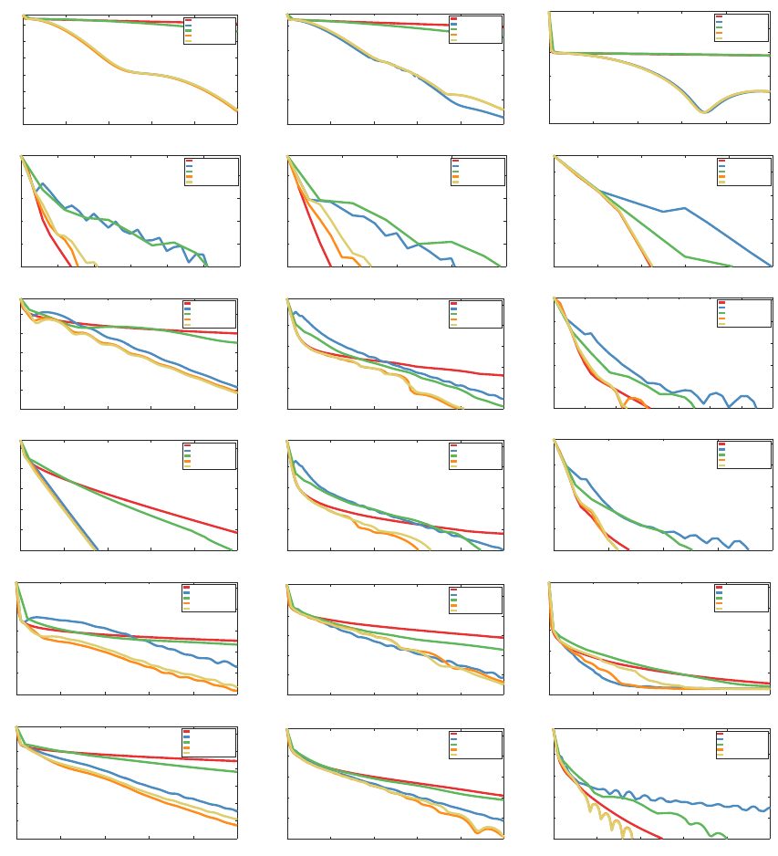
Lin, Mairal and Harchaoui

5.3 Comparison of Stopping Criteria and Warm-start Strategies

First, we evaluate the performance of the previous strategies when applying Catalyst to

SVRG, SAGA and MISO. The results are presented in Figures 1, 2, and 3, respectively.

0 20 40 60 80 100

Number of gradient evaluations

-4

-3.5

-3

-2.5

-2

-1.5

-1

Relative function value gap (log scale)

covtype, logistic, µ= 1/(2

SVRG

Catalyst-SVRG C1

Catalyst-SVRG C2

Catalyst-SVRG C3

Catalyst-SVRG C1

∗

0 20 40 60 80 100

Number of gradient evaluations

-10

-8

-6

-4

-2

Relative function value gap (log scale)

covtype, elasticnet, µ=1/100 n, λ=1/n

SVRG

Catalyst-SVRG C1

Catalyst-SVRG C2

Catalyst-SVRG C3

Catalyst-SVRG C1

∗

0 20 40 60 80 100

Number of gradient evaluations

-6

-5

-4

-3

-2

Relative function value gap (log scale)

covtype, lasso, λ= 10 / n

SVRG

Catalyst-SVRG C1

Catalyst-SVRG C2

Catalyst-SVRG C3

Catalyst-SVRG C1

∗

0 5 10 15 20 25 30

Number of gradient evaluations

-10

-8

-6

-4

-2

Relative function value gap (log scale)

alpha, logistic, µ= 1/(2

SVRG

Catalyst-SVRG C1

Catalyst-SVRG C2

Catalyst-SVRG C3

Catalyst-SVRG C1

∗

0 5 10 15 20

Number of gradient evaluations

-10

-8

-6

-4

-2

Relative function value gap (log scale)

alpha, elasticnet, µ=1/100 n, λ=1/n

SVRG

Catalyst-SVRG C1

Catalyst-SVRG C2

Catalyst-SVRG C3

Catalyst-SVRG C1

∗

0 2 4 6 8 10

Number of gradient evaluations

-10

-8

-6

-4

-2

Relative function value gap (log scale)

alpha, lasso, λ= 100 / n

SVRG

Catalyst-SVRG C1

Catalyst-SVRG C2

Catalyst-SVRG C3

Catalyst-SVRG C1

∗

0 20 40 60 80 100

Number of gradient evaluations

-10

-8

-6

-4

-2

Relative function value gap (log scale)

real-sim, logistic, µ= 1/(2

SVRG

Catalyst-SVRG C1

Catalyst-SVRG C2

Catalyst-SVRG C3

Catalyst-SVRG C1

∗

0 20 40 60 80 100

Number of gradient evaluations

-10

-8

-6

-4

-2

Relative function value gap (log scale)

real-sim, elasticnet, µ=1/100 n, λ=1/n

SVRG

Catalyst-SVRG C1

Catalyst-SVRG C2

Catalyst-SVRG C3

Catalyst-SVRG C1

∗

0 5 10 15 20 25 30 35

Number of gradient evaluations

-10

-8

-6

-4

-2

Relative function value gap (log scale)

real-sim, lasso, λ= 10 / n

SVRG

Catalyst-SVRG C1

Catalyst-SVRG C2

Catalyst-SVRG C3

Catalyst-SVRG C1

∗

0 20 40 60 80 100

Number of gradient evaluations

-10

-8

-6

-4

-2

Relative function value gap (log scale)

rcv1, logistic, µ= 1/(2

SVRG

Catalyst-SVRG C1

Catalyst-SVRG C2

Catalyst-SVRG C3

Catalyst-SVRG C1

∗

0 20 40 60 80 100

Number of gradient evaluations

-10

-8

-6

-4

-2

Relative function value gap (log scale)

rcv1, elasticnet, µ=1/100 n, λ=1/n

SVRG

Catalyst-SVRG C1

Catalyst-SVRG C2

Catalyst-SVRG C3

Catalyst-SVRG C1

∗

0 10 20 30 40

Number of gradient evaluations

-10

-8

-6

-4

-2

Relative function value gap (log scale)

rcv1, lasso, λ= 10 / n

SVRG

Catalyst-SVRG C1

Catalyst-SVRG C2

Catalyst-SVRG C3

Catalyst-SVRG C1

∗

0 20 40 60 80 100

Number of gradient evaluations

-3

-2

-1

Relative function value gap (log scale)

Image Features from MNIST, logistic, µ= 1/(2

SVRG

Catalyst-SVRG C1

Catalyst-SVRG C2

Catalyst-SVRG C3

Catalyst-SVRG C1

∗

0 20 40 60 80 100

Number of gradient evaluations

-10

-8

-6

-4

-2

Relative function value gap (log scale)

Image Features from MNIST, elasticnet, µ=1/100 n, λ=1/n

SVRG

Catalyst-SVRG C1

Catalyst-SVRG C2

Catalyst-SVRG C3

Catalyst-SVRG C1

∗

0 20 40 60 80 100

Number of gradient evaluations

-4

-3

-2

-1

Relative function value gap (log scale)

Image Features from MNIST, lasso, λ= 1 / n

SVRG

Catalyst-SVRG C1

Catalyst-SVRG C2

Catalyst-SVRG C3

Catalyst-SVRG C1

∗

0 20 40 60 80 100

Number of gradient evaluations

-5

-4

-3

-2

-1

Relative function value gap (log scale)

Image Features from CIFAR, logistic, µ= 1/(2

SVRG

Catalyst-SVRG C1

Catalyst-SVRG C2

Catalyst-SVRG C3

Catalyst-SVRG C1

∗

0 20 40 60 80 100

Number of gradient evaluations

-10

-8

-6

-4

-2

Relative function value gap (log scale)

Image Features from CIFAR, elasticnet, µ=1/100 n, λ=1/n

SVRG

Catalyst-SVRG C1

Catalyst-SVRG C2

Catalyst-SVRG C3

Catalyst-SVRG C1

∗

0 20 40 60 80 100

Number of gradient evaluations

-10

-8

-6

-4

-2

Relative function value gap (log scale)

Image Features from CIFAR, lasso, λ= 10 / n

SVRG

Catalyst-SVRG C1

Catalyst-SVRG C2

Catalyst-SVRG C3

Catalyst-SVRG C1

∗

Figure 1: Experimental study of diﬀerent stopping criterions for Catalyst-SVRG. We plot

the value f (x

)/f

∗

− 1 as a function of the number of gradient evaluations, on a

logarithmic scale; the optimal value f

∗

is estimated with a duality gap.

Catalyst for First-order Convex Optimization

Observations for Catalyst-SVRG. We remark that in most of the cases, the curve of

(C3) and (C1

∗

)are superimposed, meaning that one pass through the data is enough for solv-

ing the subproblem up to the required accuracy. Moreover, they give the best performance

among all criterions. Regarding the logistic regression problem, the acceleration is signif-

icant (even huge for the covtype data set) except for alpha, where only (C3) and (C1

∗

)do

not degrade signiﬁcantly the performance. For sparse problems, the eﬀect of acceleration

is more mitigated, with 7 cases out of 12 exhibiting important acceleration and 5 cases no

acceleration. As before, (C3) and (C1

∗

)are the only strategies that never degrade perfor-

mance.

One reason explaining why acceleration is not systematic may be the ability of incre-

mental methods to adapt to the unknown strong convexity parameter µ

≥ µ hidden in the

objective’s loss, or local strong convexity near the solution. When µ

/L ≥ 1/n, we indeed

obtain a well-conditioned regime where acceleration should not occur theoretically. In fact

the complexity O(n log(1/ε)) is already optimal in this regime, see Arjevani and Shamir

(2016); Woodworth and Srebro (2016). For sparse problems, conditioning of the problem

with respect to the linear subspace where the solution lies might also play a role, even

though our analysis does not study this aspect. Therefore, this experiment suggests that

adaptivity to unknown strong convexity is of high interest for incremental optimization.

Observations for Catalyst-SAGA. Our conclusions with SAGA are almost the same

as with SVRG. However, in a few cases, we also notice that criterion C1 lacks stability,

or at least exhibits some oscillations, which may suggest that SAGA has a larger variance

compared to SVRG. The diﬀerence in the performance of (C1) and (C1

∗

)can be huge, while

they diﬀer from each other only by the warm start strategy. Thus, choosing a good initial

point for solving the sub-problems is a key for obtaining acceleration in practice.

Observations for Catalyst-MISO. The warm-start strategy of MISO is diﬀerent from

primal algorithms because parameters for the dual function need to be speciﬁed. The most

natural way for warm starting the dual functions is to set

k+1

(x) = d

(x) +

kx − y

−

kx − y

k−1

where d

is the last dual function of the previous subproblem h

. This gives the warm start

= prox



κ + µ

− y

k−1

)



For other choices of z

, the dual function needs to be recomputed from scratch, which is com-

putationally expensive and unstable for ill-conditioned problems. Thus, we only present the

experimental results with respect to criterion (C1) and the one-pass heuristic (C3) . As we

observe, a huge acceleration is obtained in logistic regression and Elastic-net formulations.

For Lasso problem, the original Prox-MISO is not deﬁned since the problem is not strongly

convex. Thus, in order to make a comparison, we compare with Catalyst-SVRG which

shows that the acceleration achieves a similar performance. This aligns with the theoretical

result stating that Catalyst applied to incremental algorithms yields a similar convergence

rate. Notice also that the original MISO algorithm suﬀers from numerical stability in this

ill-conditioned regime chosen for our experiments. Catalyst not only accelerates MISO, but

it also stabilizes it.

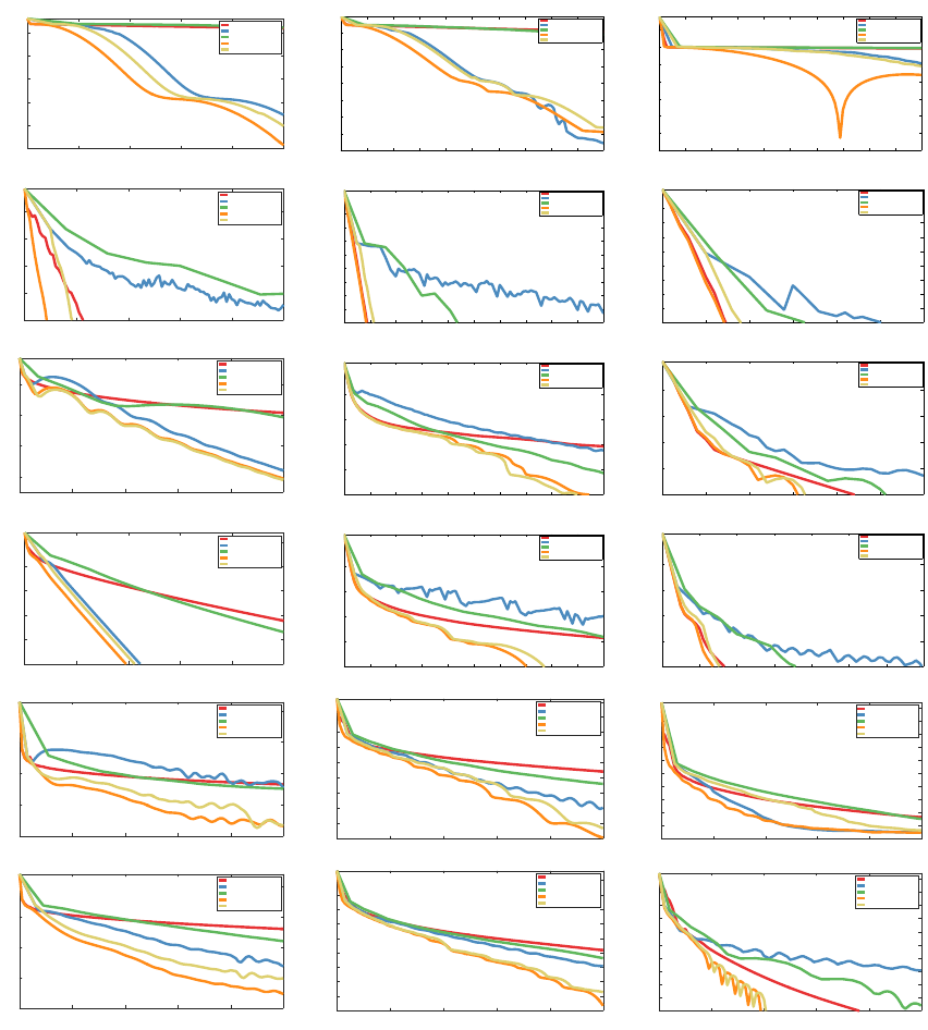
Lin, Mairal and Harchaoui

0 20 40 60 80 100

Number of gradient evaluations

-3.5

-3

-2.5

-2

-1.5

-1

Relative function value gap (log scale)

covtype, logistic, µ= 1/(2

SAGA

Catalyst-SAGA C1

Catalyst-SAGA C2

Catalyst-SAGA C3

Catalyst-SAGA C1

∗

0 10 20 30 40 50 60 70 80 90 100

−9

−8

−7

−6

−5

−4

−3

−2

Number of gradient evaluations

Relative function value gap

covtype, elasticnet, µ=1/100 n, λ=1/n

SAGA

Catalyst-SAGA C1

Catalyst-SAGA C2

Catalyst-SAGA C3

Catalyst-SAGA C1

∗

0 10 20 30 40 50 60 70 80 90 100

−9

−8

−7

−6

−5

−4

−3

−2

Number of gradient evaluations

Relative function value gap

covtype, lasso, λ= 10 / n

SAGA

Catalyst-SAGA C1

Catalyst-SAGA C2

Catalyst-SAGA C3

Catalyst-SAGA C1

∗

0 20 40 60 80 100

Number of gradient evaluations

-10

-8

-6

-4

-2

Relative function value gap (log scale)

alpha, logistic, µ= 1/(2

SAGA

Catalyst-SAGA C1

Catalyst-SAGA C2

Catalyst-SAGA C3

Catalyst-SAGA C1

∗

0 10 20 30 40 50 60 70 80 90 100

−10

−9

−8

−7

−6

−5

−4

−3

−2

−1

Number of gradient evaluations

Relative function value gap

alpha, elasticnet, µ=1/100 n, λ=1/n

SAGA

Catalyst-SAGA C1

Catalyst-SAGA C2

Catalyst-SAGA C3

Catalyst-SAGA C1

∗

0 5 10 15 20 25 30

−10

−9

−8

−7

−6

−5

−4

−3

−2

−1

Number of gradient evaluations

Relative function value gap

alpha, lasso, λ= 100 / n

SAGA

Catalyst-SAGA C1

Catalyst-SAGA C2

Catalyst-SAGA C3

Catalyst-SAGA C1

∗

0 20 40 60 80 100

Number of gradient evaluations

-6

-4

-2

Relative function value gap (log scale)

real-sim, logistic, µ= 1/(2

SAGA

Catalyst-SAGA C1

Catalyst-SAGA C2

Catalyst-SAGA C3

Catalyst-SAGA C1

∗

0 10 20 30 40 50 60 70 80 90 100

−10

−8

−6

−4

−2

Number of gradient evaluations

Relative function value gap

real-sim, elasticnet, µ=1/100 n, λ=1/n

SAGA

Catalyst-SAGA C1

Catalyst-SAGA C2

Catalyst-SAGA C3

Catalyst-SAGA C1

∗

0 5 10 15 20 25 30

−10

−8

−6

−4

−2

Number of gradient evaluations

Relative function value gap

real-sim, lasso, λ= 10 / n

SAGA

Catalyst-SAGA C1

Catalyst-SAGA C2

Catalyst-SAGA C3

Catalyst-SAGA C1

∗

0 20 40 60 80 100

Number of gradient evaluations

-10

-8

-6

-4

-2

Relative function value gap (log scale)

rcv1, logistic, µ= 1/(2

SAGA

Catalyst-SAGA C1

Catalyst-SAGA C2

Catalyst-SAGA C3

Catalyst-SAGA C1

∗

0 10 20 30 40 50 60 70 80 90 100

−10

−8

−6

−4

−2

Number of gradient evaluations

Relative function value gap

rcv1, elasticnet, µ=1/100 n, λ=1/n

SAGA

Catalyst-SAGA C1

Catalyst-SAGA C2

Catalyst-SAGA C3

Catalyst-SAGA C1

∗

0 10 20 30 40 50 60 70

−10

−8

−6

−4

−2

Number of gradient evaluations

Relative function value gap

rcv1, lasso, λ= 10 / n

SAGA

Catalyst-SAGA C1

Catalyst-SAGA C2

Catalyst-SAGA C3

Catalyst-SAGA C1

∗

0 20 40 60 80 100

Number of gradient evaluations

-2

-1

Relative function value gap (log scale)

Image Features from MNIST, logistic, µ= 1/(2

SAGA

Catalyst-SAGA C1

Catalyst-SAGA C2

Catalyst-SAGA C3

Catalyst-SAGA C1

∗

0 20 40 60 80 100

Number of gradient evaluations

-8

-7

-6

-5

-4

-3

-2

-1

Relative function value gap (log scale)

Image Features from MNIST, elasticnet, µ=1/100 n, λ=1/n

SAGA

Catalyst-SAGA C1

Catalyst-SAGA C2

Catalyst-SAGA C3

Catalyst-SAGA C1

∗

0 20 40 60 80 100

Number of gradient evaluations

-4

-3.5

-3

-2.5

-2

-1.5

-1

-0.5

0.5

Relative function value gap (log scale)

Image Features from MNIST, lasso, λ= 1 / n

SAGA

Catalyst-SAGA C1

Catalyst-SAGA C2

Catalyst-SAGA C3

Catalyst-SAGA C1

∗

0 20 40 60 80 100

Number of gradient evaluations

-3

-2

-1

Relative function value gap (log scale)

Image Features from CIFAR, logistic, µ= 1/(2

SAGA

Catalyst-SAGA C1

Catalyst-SAGA C2

Catalyst-SAGA C3

Catalyst-SAGA C1

∗

0 20 40 60 80 100

Number of gradient evaluations

-9

-8

-7

-6

-5

-4

-3

-2

-1

Relative function value gap (log scale)

Image Features from CIFAR, elasticnet, µ=1/100 n, λ=1/n

SAGA

Catalyst-SAGA C1

Catalyst-SAGA C2

Catalyst-SAGA C3

Catalyst-SAGA C1

∗

0 20 40 60 80 100

Number of gradient evaluations

-10

-9

-8

-7

-6

-5

-4

-3

-2

-1

Relative function value gap (log scale)

Image Features from CIFAR, lasso, λ= 10 / n

SAGA

Catalyst-SAGA C1

Catalyst-SAGA C2

Catalyst-SAGA C3

Catalyst-SAGA C1

∗

Figure 2: Experimental study of diﬀerent stopping criterions for Catalyst-SAGA, with a

similar setting as in Figure 1.

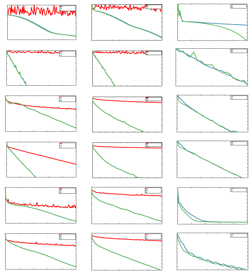
Catalyst for First-order Convex Optimization

0 20 40 60 80 100

Number of gradient evaluations

-3

-2.5

-2

-1.5

-1

-0.5

Relative function value gap

covtype, logistic, µ= 1/(2

MISO

Catalyst-MISO C1

Catalyst-MISO C3

0 10 20 30 40 50 60 70 80 90 100

−8

−7

−6

−5

−4

−3

−2

−1

Number of gradient evaluations

Relative function value gap

covtype, elasticnet, µ=1/100 n, λ=1/n

MISO

Catalyst-MISO C1

Catalyst-MISO C3

0 20 40 60 80 100

Number of gradient evaluations

-5.5

-5

-4.5

-4

-3.5

-3

-2.5

-2

-1.5

-1

Relative function value gap

covtype, lasso, λ= 10 / n

Catalyst-MISO C1

Catalyst-MISO C3

0 20 40 60 80 100

Number of gradient evaluations

-10

-8

-6

-4

-2

Relative function value gap

alpha, logistic, µ= 1/(2

MISO

Catalyst-MISO C1

Catalyst-MISO C3

0 10 20 30 40 50 60 70 80 90 100

−10

−9

−8

−7

−6

−5

−4

−3

−2

−1

Number of gradient evaluations

Relative function value gap

alpha, elasticnet, µ=1/100 n, λ=1/n

MISO

Catalyst-MISO C1

Catalyst-MISO C3

0 5 10 15 20

Number of gradient evaluations

-8

-7

-6

-5

-4

-3

-2

-1

Relative function value gap

alpha, lasso, λ= 100 / n

Catalyst-MISO C1

Catalyst-MISO C3

0 20 40 60 80 100

Number of gradient evaluations

-8

-6

-4

-2

Relative function value gap

real-sim, logistic, µ= 1/(2

MISO

Catalyst-MISO C1

Catalyst-MISO C3

0 10 20 30 40 50 60 70 80 90 100

−10

−8

−6

−4

−2

Number of gradient evaluations

Relative function value gap

real-sim, elasticnet, µ=1/100 n, λ=1/n

MISO

Catalyst-MISO C1

Catalyst-MISO C3

0 5 10 15 20 25 30

Number of gradient evaluations

-10

-9

-8

-7

-6

-5

-4

-3

-2

-1

Relative function value gap

real-sim, lasso, λ= 10 / n

Catalyst-MISO C1

Catalyst-MISO C3

0 20 40 60 80 100

Number of gradient evaluations

-10

-8

-6

-4

-2

Relative function value gap

rcv1, logistic, µ= 1/(2

MISO

Catalyst-MISO C1

Catalyst-MISO C3

0 10 20 30 40 50 60 70 80 90 100

−10

−8

−6

−4

−2

Number of gradient evaluations

Relative function value gap

rcv1, elasticnet, µ=1/100 n, λ=1/n

MISO

Catalyst-MISO C1

Catalyst-MISO C3

0 5 10 15 20 25 30

Number of gradient evaluations

-10

-9

-8

-7

-6

-5

-4

-3

-2

-1

Relative function value gap

rcv1, lasso, λ= 10 / n

Catalyst-MISO C1

Catalyst-MISO C3

0 20 40 60 80 100

Number of gradient evaluations

-2

-1

Relative function value gap

Image Features from MNIST, logistic, µ= 1/(2

MISO

Catalyst-MISO C1

Catalyst-MISO C3

0 20 40 60 80 100

Number of gradient evaluations

-10

-8

-6

-4

-2

Relative function value gap

Image Features from MNIST, elasticnet, µ=1/100 n, λ=1/n

MISO

Catalyst-MISO C1

Catalyst-MISO C3

0 20 40 60 80 100

Number of gradient evaluations

-4

-3.5

-3

-2.5

-2

-1.5

-1

-0.5

0.5

Relative function value gap

Image Features from MNIST, lasso, λ= 1 / n

Catalyst-MISO C1

Catalyst-MISO C3

0 20 40 60 80 100

Number of gradient evaluations

-4

-3

-2

-1

Relative function value gap

Image Features from CIFAR, logistic, µ= 1/(2

MISO

Catalyst-MISO C1

Catalyst-MISO C3

0 20 40 60 80 100

Number of gradient evaluations

-10

-9

-8

-7

-6

-5

-4

-3

-2

-1

Relative function value gap

Image Features from CIFAR, elasticnet, µ=1/100 n, λ=1/n

MISO

Catalyst-MISO C1

Catalyst-MISO C3

0 10 20 30 40 50 60 70

Number of gradient evaluations

-10

-9

-8

-7

-6

-5

-4

-3

-2

-1

Relative function value gap

Image Features from CIFAR, lasso, λ= 10 / n

Catalyst-MISO C1

Catalyst-MISO C3

Figure 3: Experimental study of diﬀerent stopping criterions for Catalyst-MISO, with a

similar setting as in Figure 1

Lin, Mairal and Harchaoui

5.4 Acceleration of Existing Methods

Then, we put the previous curves into perspective and make a comparison of the perfor-

mance before and after applying Catalyst across methods. We show the best performance

among the three developed stopping criteria, which corresponds to be (C3) .

Observations. In Figure 4, we observe that by applying Catalyst, we accelerate the

original algorithms up to the limitations discussed above (comparing the dashed line and

the solid line of the same color). In three data sets (covtype, real-sim and rcv1), signiﬁcant

improvements are achieved as expected by the theory for the ill-conditioned problems in

logistic regression and Elastic-net. For data set alpha, we remark that an relative accuracy

in the order 10

−10

is attained in less than 10 iterations. This suggests that the problems is

in fact well-conditioned and there is some hidden strong convexity for this data set. Thus,

the incremental algorithms like SVRG or SAGA are already optimal under this situation

and no further improvement can be obtained by applying Catalyst.

5.5 Empirical Eﬀect on the Generalization Error

A natural question that applies to all incremental methods is whether or not the acceleration

that we may see for minimizing an empirical risk on training data aﬀects the objective

function and the test accuracy on new unseen test data. To answer this question, we

consider the logistic regression formulation with the regularization parameter µ

∗

obtained

by cross-validation. Then, we cut each data set into 80% of training data and set aside 20%

of the data point as test data.

Observations on the test loss and test accuracy. The left column of Figure 5 shows

the loss function on the training set, where acceleration is signiﬁcant in 5 cases out of 6. The

middle column shows the loss function evaluated on the test set, but on a non-logarithmic

scale since the optimal value of the test loss is unknown. Acceleration appears in 4 cases

out of 6. Regarding the test accuracy, an important acceleration is obtained in 2 cases,

whereas it is less signiﬁcant or negligible in the other cases.

5.6 Study of the Parameter κ

Finally, we evaluate the performance for diﬀerent values of κ.

Observations for diﬀerent choices of κ. We consider a logarithmic grid κ = 10

with i = −2, −1, ··· , 2 and κ

is the optimal κ given by the theory. We observe that for ill-

conditioned problems, using optimal choice κ

provides much better performance than other

choices, which conﬁrms the theoretical result. For the data set of alpha or Lasso problems,

we observe that the best choice is given by the smallest κ = 0.01κ

. This suggests that, as

discussed before, there is a certain degree of strong convexity present in the objective even

without any regularization.

6. Conclusion

We have introduced a generic algorithm called Catalyst that allows us to extend Nesterov’s

acceleration to a large class of ﬁrst-order methods. We have shown that it can be eﬀective

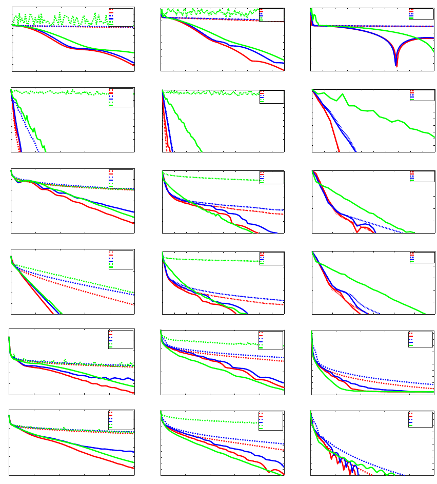
Catalyst for First-order Convex Optimization

0 20 40 60 80 100

Number of gradient evaluations

-4

-3.5

-3

-2.5

-2

-1.5

-1

-0.5

0.5

Relative function value gap

covtype, logistic, µ= 1/(2

SVRG

Catalyst-SVRG

SAGA

Catalyst-SAGA

MISO

Catalyst-MISO

0 10 20 30 40 50 60 70 80 90 100

−9

−8

−7

−6

−5

−4

−3

−2

−1

Number of gradient evaluations

Relative function value gap

covtype, elasticnet, µ=1/100 n, λ=1/n

SVRG

Catalyst-SVRG

SAGA

Catalyst-SAGA

MISO

Catalyst-MISO

0 10 20 30 40 50 60 70 80 90 100

−9

−8

−7

−6

−5

−4

−3

−2

−1

Number of gradient evaluations

Relative function value gap

covtype, lasso, λ= 10 / n

SVRG

Catalyst-SVRG

SAGA

Catalyst-SAGA

Catalyst-MISO

0 20 40 60 80 100

Number of gradient evaluations

-10

-9

-8

-7

-6

-5

-4

-3

-2

-1

Relative function value gap

alpha, logistic, µ= 1/(2

SVRG

Catalyst-SVRG

SAGA

Catalyst-SAGA

MISO

Catalyst-MISO

0 10 20 30 40 50 60 70 80 90 100

−10

−9

−8

−7

−6

−5

−4

−3

−2

−1

Number of gradient evaluations

Relative function value gap

alpha, elasticnet, µ=1/100 n, λ=1/n

SVRG

Catalyst-SVRG

SAGA

Catalyst-SAGA

MISO

Catalyst-MISO

0 2 4 6 8 10 12 14 16 18 20

−10

−9

−8

−7

−6

−5

−4

−3

−2

−1

Number of gradient evaluations

Relative function value gap

alpha, lasso, λ= 100 / n

SVRG

Catalyst-SVRG

SAGA

Catalyst-SAGA

Catalyst-MISO

0 20 40 60 80 100

Number of gradient evaluations

-10

-8

-6

-4

-2

Relative function value gap

real-sim, logistic, µ= 1/(2

SVRG

Catalyst-SVRG

SAGA

Catalyst-SAGA

MISO

Catalyst-MISO

0 10 20 30 40 50 60 70 80 90 100

−10

−8

−6

−4

−2

Number of gradient evaluations

Relative function value gap

real-sim, elasticnet, µ=1/100 n, λ=1/n

SVRG

Catalyst-SVRG

SAGA

Catalyst-SAGA

MISO

Catalyst-MISO

0 5 10 15 20 25 30

−10

−8

−6

−4

−2

Number of gradient evaluations

Relative function value gap

real-sim, lasso, λ= 10 / n

SVRG

Catalyst-SVRG

SAGA

Catalyst-SAGA

Catalyst-MISO

0 20 40 60 80 100

Number of gradient evaluations

-10

-8

-6

-4

-2

Relative function value gap

rcv1, logistic, µ= 1/(2

SVRG

Catalyst-SVRG

SAGA

Catalyst-SAGA

MISO

Catalyst-MISO

0 10 20 30 40 50 60 70 80 90 100

−10

−8

−6

−4

−2

Number of gradient evaluations

Relative function value gap

rcv1, elasticnet, µ=1/100 n, λ=1/n

SVRG

Catalyst-SVRG

SAGA

Catalyst-SAGA

MISO

Catalyst-MISO

0 5 10 15 20 25 30

−10

−8

−6

−4

−2

Number of gradient evaluations

Relative function value gap

rcv1, lasso, λ= 10 / n

SVRG

Catalyst-SVRG

SAGA

Catalyst-SAGA

Catalyst-MISO

0 20 40 60 80 100

Number of gradient evaluations

-3

-2

-1

Relative function value gap

mnist, logistic, µ= 1/(2

SVRG

Catalyst-SVRG

SAGA

Catalyst-SAGA

MISO

Catalyst-MISO

0 20 40 60 80 100

Number of gradient evaluations

-10

-8

-6

-4

-2

Relative function value gap

mnist, elasticnet, µ=1/100 n, λ=1/n

SVRG

Catalyst-SVRG

SAGA

Catalyst-SAGA

MISO

Catalyst-MISO

0 20 40 60 80 100

Number of gradient evaluations

-4

-3.5

-3

-2.5

-2

-1.5

-1

-0.5

0.5

Relative function value gap

mnist, lasso, λ= 1 / n

SVRG

Catalyst-SVRG

SAGA

Catalyst-SAGA

Catalyst-MISO

0 20 40 60 80 100

Number of gradient evaluations

-5

-4

-3

-2

-1

Relative function value gap

hongzhou, logistic, µ= 1/(2

SVRG

Catalyst-SVRG

SAGA

Catalyst-SAGA

MISO

Catalyst-MISO

0 20 40 60 80 100

Number of gradient evaluations

-10

-9

-8

-7

-6

-5

-4

-3

-2

-1

Relative function value gap

hongzhou, elasticnet, µ=1/100 n, λ=1/n

SVRG

Catalyst-SVRG

SAGA

Catalyst-SAGA

MISO

Catalyst-MISO

0 20 40 60 80 100

Number of gradient evaluations

-10

-9

-8

-7

-6

-5

-4

-3

-2

-1

Relative function value gap

hongzhou, lasso, λ= 10 / n

SVRG

Catalyst-SVRG

SAGA

Catalyst-SAGA

Catalyst-MISO

Figure 4: Experimental study of the performance of Catalyst applying to SVRG, SAGA and

MISO. The dashed lines correspond to the original algorithms and the solid lines

correspond to accelerated algorithms by applying Catalyst. We plot the relative

function value gap (f (x

) − f

∗

)/f

∗

in the number of gradient evaluations, on a

logarithmic scale.

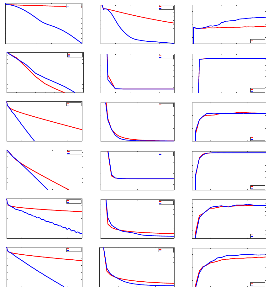
Lin, Mairal and Harchaoui

0 20 40 60 80 100

Number of gradient evaluations

-9

-8

-7

-6

-5

-4

-3

-2

Relative function value gap (log scale)

covtype, logistic, µ= 0.00195312/n

SVRG

Catalyst-SVRG

0 10 20 30 40 50

Number of gradient evaluations

0.66

0.661

0.662

0.663

0.664

0.665

0.666

0.667

0.668

0.669

0.67

Test loss

covtype, logistic, µ= 0.00195312/n

SVRG

Catalyst-SVRG

0 10 20 30 40 50

Number of gradient evaluations

0.58

0.585

0.59

0.595

0.6

0.605

0.61

Test Accuracy

covtype, logistic, µ= 0.00195312/n

SVRG

Catalyst-SVRG

0 1 2 3 4 5 6 7 8

Number of gradient evaluations

-10

-9

-8

-7

-6

-5

-4

-3

-2

-1

Relative function value gap (log scale)

alpha, logistic, µ= 0.015625/n

SVRG

Catalyst-SVRG

0 2 4 6 8 10

Number of gradient evaluations

0.465

0.47

0.475

0.48

0.485

0.49

0.495

0.5

Test loss

alpha, logistic, µ= 0.015625/n

SVRG

Catalyst-SVRG

0 2 4 6 8 10

Number of gradient evaluations

0.75

0.755

0.76

0.765

0.77

0.775

0.78

0.785

Test Accuracy

alpha, logistic, µ= 0.015625/n

SVRG

Catalyst-SVRG

0 20 40 60 80 100

Number of gradient evaluations

-10

-8

-6

-4

-2

Relative function value gap (log scale)

real-sim, logistic, µ= 0.03125/n

SVRG

Catalyst-SVRG

0 5 10 15 20

Number of gradient evaluations

0.07

0.075

0.08

0.085

0.09

0.095

0.1

Test loss

real-sim, logistic, µ= 0.03125/n

SVRG

Catalyst-SVRG

0 5 10 15 20

Number of gradient evaluations

0.95

0.955

0.96

0.965

0.97

0.975

0.98

Test Accuracy

real-sim, logistic, µ= 0.03125/n

SVRG

Catalyst-SVRG

0 5 10 15 20 25

Number of gradient evaluations

-10

-9

-8

-7

-6

-5

-4

-3

-2

-1

Relative function value gap (log scale)

rcv1, logistic, µ= 0.25/n

SVRG

Catalyst-SVRG

0 5 10 15 20

Number of gradient evaluations

0.128

0.129

0.13

0.131

0.132

0.133

0.134

0.135

Test loss

rcv1, logistic, µ= 0.25/n

SVRG

Catalyst-SVRG

0 5 10 15 20

Number of gradient evaluations

0.94

0.942

0.944

0.946

0.948

0.95

0.952

Test Accuracy

rcv1, logistic, µ= 0.25/n

SVRG

Catalyst-SVRG

0 20 40 60 80 100

Number of gradient evaluations

-10

-8

-6

-4

-2

Relative function value gap (log scale)

Image feature from MNIST, logistic, µ= 0.00390625/n

SVRG

Catalyst-SVRG

0 5 10 15 20

Number of gradient evaluations

0.004

0.006

0.008

0.01

0.012

0.014

0.016

0.018

0.02

Test loss

Image feature from MNIST, logistic, µ= 0.00390625/n

SVRG

Catalyst-SVRG

0 5 10 15 20

Number of gradient evaluations

0.99

0.991

0.992

0.993

0.994

0.995

0.996

0.997

0.998

0.999

Test Accuracy

Image feature from MNIST, logistic, µ= 0.00390625/n

SVRG

Catalyst-SVRG

0 20 40 60 80 100

Number of gradient evaluations

-10

-8

-6

-4

-2

Relative function value gap (log scale)

Image feature from CIFAR, logistic, µ= 0.0078125/n

SVRG

Catalyst-SVRG

0 5 10 15 20

Number of gradient evaluations

0.07

0.08

0.09

0.1

0.11

0.12

0.13

0.14

0.15

Test loss

Image feature from CIFAR, logistic, µ= 0.0078125/n

SVRG

Catalyst-SVRG

0 5 10 15 20

Number of gradient evaluations

0.95

0.955

0.96

0.965

0.97

0.975

0.98

Test Accuracy

Image feature from CIFAR, logistic, µ= 0.0078125/n

SVRG

Catalyst-SVRG

Figure 5: Empirical eﬀect on the generalization error. For a logistic regression experiment,

we report the value of the objective function evaluated on the training data on

the left column, the value of the loss evaluated on a test set on the middle column,

and the classiﬁcation error evaluated on the test set on the right.

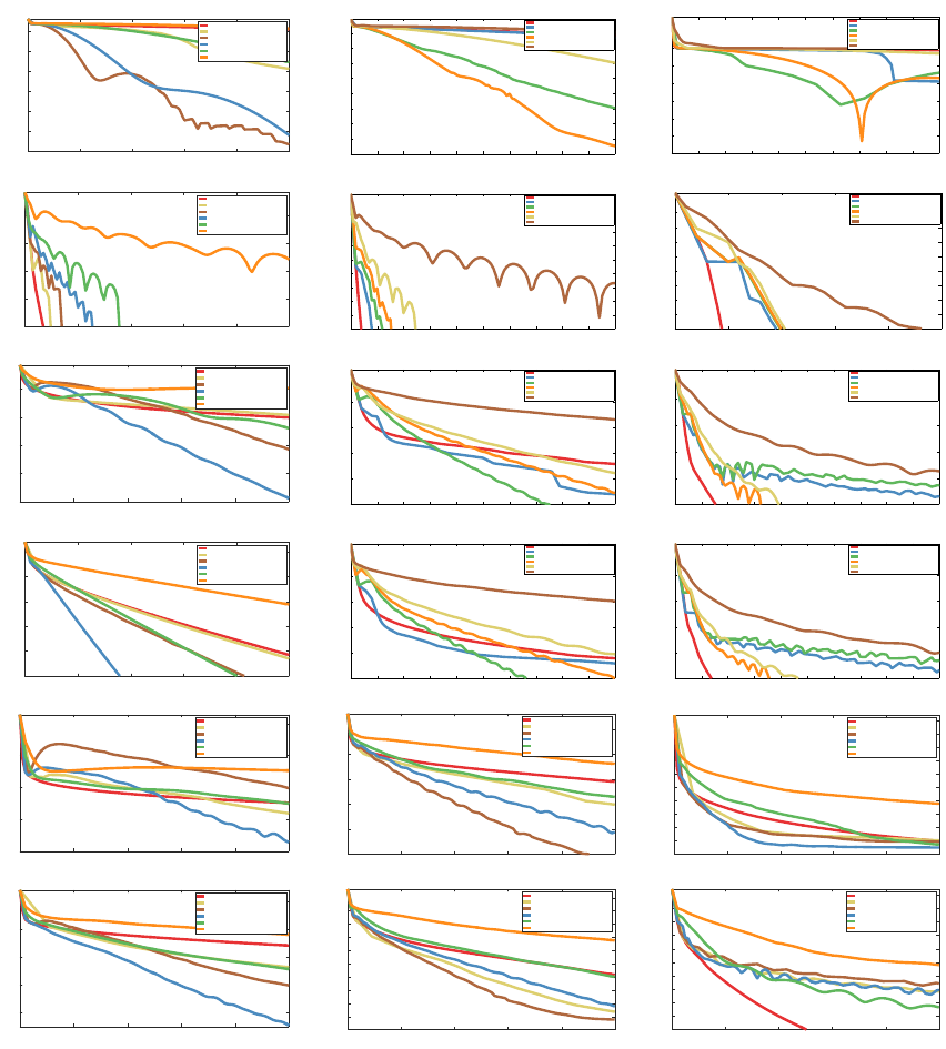
Catalyst for First-order Convex Optimization

0 20 40 60 80 100

Number of gradient evaluations

-4

-3.5

-3

-2.5

-2

-1.5

-1

Relative function value gap

covtype, logistic, µ= 1/(2

SVRG

Catalyst-SVRG C1 κ=0.01 κ

Catalyst-SVRG C1 κ=0.1 κ

Catalyst-SVRG C1 κ=1 κ

Catalyst-SVRG C1 κ=10 κ

Catalyst-SVRG C1 κ=100 κ

0 10 20 30 40 50 60 70 80 90 100

−10

−9

−8

−7

−6

−5

−4

−3

−2

Number of gradient evaluations

Relative function value gap

covtype, elasticnet, µ=1/100 n, λ=1/n

SVRG

Catalyst-SVRG C1 κ=0.01 κ

Catalyst-SVRG C1 κ=0.1 κ

Catalyst-SVRG C1 κ=1 κ

Catalyst-SVRG C1 κ=10 κ

Catalyst-SVRG C1 κ=100 κ

0 10 20 30 40 50 60 70 80 90 100

−9

−8

−7

−6

−5

−4

−3

−2

Number of gradient evaluations

Relative function value gap

covtype, lasso, λ= 10 / n

SVRG

Catalyst-SVRG C1 κ=0.01 κ

Catalyst-SVRG C1 κ=0.1 κ

Catalyst-SVRG C1 κ=1 κ

Catalyst-SVRG C1 κ=10 κ

Catalyst-SVRG C1 κ=100 κ

0 20 40 60 80 100

Number of gradient evaluations

-10

-8

-6

-4

-2

Relative function value gap

alpha, logistic, µ= 1/(2

SVRG

Catalyst-SVRG C1 κ=0.01 κ

Catalyst-SVRG C1 κ=0.1 κ

Catalyst-SVRG C1 κ=1 κ

Catalyst-SVRG C1 κ=10 κ

Catalyst-SVRG C1 κ=100 κ

0 10 20 30 40 50 60 70 80 90 100

−10

−9

−8

−7

−6

−5

−4

−3

−2

−1

Number of gradient evaluations

Relative function value gap

alpha, elasticnet, µ=1/100 n, λ=1/n

SVRG

Catalyst-SVRG C1 κ=0.01 κ

Catalyst-SVRG C1 κ=0.1 κ

Catalyst-SVRG C1 κ=1 κ

Catalyst-SVRG C1 κ=10 κ

Catalyst-SVRG C1 κ=100 κ

0 5 10 15 20 25

−10

−9

−8

−7

−6

−5

−4

−3

−2

−1

Number of gradient evaluations

Relative function value gap

alpha, lasso, λ= 100 / n

SVRG

Catalyst-SVRG C1 κ=0.01 κ

Catalyst-SVRG C1 κ=0.1 κ

Catalyst-SVRG C1 κ=1 κ

Catalyst-SVRG C1 κ=10 κ

Catalyst-SVRG C1 κ=100 κ

0 20 40 60 80 100

Number of gradient evaluations

-8

-6

-4

-2

Relative function value gap

real-sim, logistic, µ= 1/(2

SVRG

Catalyst-SVRG C1 κ=0.01 κ

Catalyst-SVRG C1 κ=0.1 κ

Catalyst-SVRG C1 κ=1 κ

Catalyst-SVRG C1 κ=10 κ

Catalyst-SVRG C1 κ=100 κ

0 10 20 30 40 50 60 70 80 90 100

−10

−8

−6

−4

−2

Number of gradient evaluations

Relative function value gap

real-sim, elasticnet, µ=1/100 n, λ=1/n

SVRG

Catalyst-SVRG C1 κ=0.01 κ

Catalyst-SVRG C1 κ=0.1 κ

Catalyst-SVRG C1 κ=1 κ

Catalyst-SVRG C1 κ=10 κ

Catalyst-SVRG C1 κ=100 κ

0 10 20 30 40 50 60 70 80 90 100

−10

−8

−6

−4

−2

Number of gradient evaluations

Relative function value gap

real-sim, lasso, λ= 10 / n

SVRG

Catalyst-SVRG C1 κ=0.01 κ

Catalyst-SVRG C1 κ=0.1 κ

Catalyst-SVRG C1 κ=1 κ

Catalyst-SVRG C1 κ=10 κ

Catalyst-SVRG C1 κ=100 κ

0 20 40 60 80 100

Number of gradient evaluations

-10

-8

-6

-4

-2

Relative function value gap

rcv1, logistic, µ= 1/(2

SVRG

Catalyst-SVRG C1 κ=0.01 κ

Catalyst-SVRG C1 κ=0.1 κ

Catalyst-SVRG C1 κ=1 κ

Catalyst-SVRG C1 κ=10 κ

Catalyst-SVRG C1 κ=100 κ

0 10 20 30 40 50 60 70 80 90 100

−10

−8

−6

−4

−2

Number of gradient evaluations

Relative function value gap

rcv1, elasticnet, µ=1/100 n, λ=1/n

SVRG

Catalyst-SVRG C1 κ=0.01 κ

Catalyst-SVRG C1 κ=0.1 κ

Catalyst-SVRG C1 κ=1 κ

Catalyst-SVRG C1 κ=10 κ

Catalyst-SVRG C1 κ=100 κ

0 10 20 30 40 50 60 70 80 90 100

−10

−8

−6

−4

−2

Number of gradient evaluations

Relative function value gap

rcv1, lasso, λ= 10 / n

SVRG

Catalyst-SVRG C1 κ=0.01 κ

Catalyst-SVRG C1 κ=0.1 κ

Catalyst-SVRG C1 κ=1 κ

Catalyst-SVRG C1 κ=10 κ

Catalyst-SVRG C1 κ=100 κ

0 20 40 60 80 100

Number of gradient evaluations

-2

-1

Relative function value gap

Image Features from MNIST, logistic, µ= 1/(2

SVRG

Catalyst-SVRG C1 κ=0.01 κ

Catalyst-SVRG C1 κ=0.1 κ

Catalyst-SVRG C1 κ=1 κ

Catalyst-SVRG C1 κ=10 κ

Catalyst-SVRG C1 κ=100 κ

0 20 40 60 80 100

Number of gradient evaluations

-10

-8

-6

-4

-2

Relative function value gap

Image Features from MNIST, elasticnet, µ=1/100 n, λ=1/n

SVRG

Catalyst-SVRG C1 κ=0.01 κ

Catalyst-SVRG C1 κ=0.1 κ

Catalyst-SVRG C1 κ=1 κ

Catalyst-SVRG C1 κ=10 κ

Catalyst-SVRG C1 κ=100 κ

0 20 40 60 80 100

Number of gradient evaluations

-4

-3.5

-3

-2.5

-2

-1.5

-1

-0.5

0.5

Relative function value gap

Image Features from MNIST, lasso, λ= 1 / n

SVRG

Catalyst-SVRG C1 κ=0.01 κ

Catalyst-SVRG C1 κ=0.1 κ

Catalyst-SVRG C1 κ=1 κ

Catalyst-SVRG C1 κ=10 κ

Catalyst-SVRG C1 κ=100 κ

0 20 40 60 80 100

Number of gradient evaluations

-3

-2

-1

Relative function value gap

Image Features from CIFAR, logistic, µ= 1/(2

SVRG

Catalyst-SVRG C1 κ=0.01 κ

Catalyst-SVRG C1 κ=0.1 κ

Catalyst-SVRG C1 κ=1 κ

Catalyst-SVRG C1 κ=10 κ

Catalyst-SVRG C1 κ=100 κ

0 20 40 60 80 100

Number of gradient evaluations

-10

-9

-8

-7

-6

-5

-4

-3

-2

-1

Relative function value gap

Image Features from CIFAR, elasticnet, µ=1/100 n, λ=1/n

SVRG

Catalyst-SVRG C1 κ=0.01 κ

Catalyst-SVRG C1 κ=0.1 κ

Catalyst-SVRG C1 κ=1 κ

Catalyst-SVRG C1 κ=10 κ

Catalyst-SVRG C1 κ=100 κ

0 20 40 60 80 100

Number of gradient evaluations

-10

-9

-8

-7

-6

-5

-4

-3

-2

-1

Relative function value gap

Image Features from CIFAR, lasso, λ= 10 / n

SVRG

Catalyst-SVRG C1 κ=0.01 κ

Catalyst-SVRG C1 κ=0.1 κ

Catalyst-SVRG C1 κ=1 κ

Catalyst-SVRG C1 κ=10 κ

Catalyst-SVRG C1 κ=100 κ

Figure 6: Evaluations of Catalyst-SVRG for diﬀerent κ using stopping criterion C1, where

is the theoretical choice given by the complexity analysis.

Lin, Mairal and Harchaoui

in practice for ill-conditioned problems. Besides acceleration, Catalyst also improves the

numerical stability of a given algorithm, by applying it to auxiliary problems that are better

conditioned than the original objective. For this reason, it also provides support to convex,

but not strongly convex objectives, to algorithms that originally require strong convexity.

We have also studied experimentally many variants to identify the ones that are the most

eﬀective and the simplest to use in practice. For incremental methods, we showed that

the “almost-parameter-free” variant, consisting in performing a single pass over the data at

every outer-loop iteration, was the most eﬀective one in practice.

Even though we have illustrated Catalyst in the context of ﬁnite-sum optimization

problems, the main feature of our approach is its versatility. Catalyst could also be applied

to other algorithms that have not been considered so far and give rise to new accelerated

algorithms.

Acknowledgments

The authors would like to thank Dmitriy Drusvyatskiy, Anatoli Juditsky, Sham Kakade,

Arkadi Nemirovski, Courtney Paquette, and Vincent Roulet for fruitful discussions. Hongzhou

Lin and Julien Mairal were supported by the ERC grant SOLARIS (# 714381) and a grant

from ANR (MACARON project ANR-14-CE23-0003-01). Zaid Harchaoui was supported by

NSF Award CCF-1740551 and the program “Learning in Machines and Brains” of CIFAR.

This work was performed while Hongzhou Lin was at Inria and Univ. Grenoble Alpes.

Appendix A. Useful Lemmas

Lemma 19 (Simple lemma on quadratic functions) For all vectors x, y, z in R

and

θ > 0,

kx − yk

≥ (1 − θ)kx − zk



1 −



kz − yk

Proof

kx − yk

= kx − z + z − yk

= kx − zk

+ kz − yk

+ 2hx −z, z − yi

= kx − zk

+ kz − yk



√

θ(x − z) +

√

(z − y)



− θkx − zk

−

kz − yk

≥ (1 − θ)kx − zk



1 −



kz − yk

Lemma 20 (Simple lemma on non-negative sequences) Consider a increasing sequence

)

k≥0

and two non-negative sequences (a

)

k≥0

and (u

)

k≥0

such that for all k,

≤ S

i=1

. (29)

Catalyst for First-order Convex Optimization

Then,

i=1

≤

i=1

. (30)

Proof This lemma is identical to the Lemma A.10 in the original Catalyst paper (Lin

et al., 2015a), inspired by a lemma of Schmidt et al. (2011) for controlling errors of inexact

proximal gradient methods.

We give here an elementary proof for completeness based on induction. The relation (30)

is obviously true for k = 0. Then, we assume it is true for k − 1 and prove the relation

for k. We remark that from (29),



−



≤ S

k−1

i=1

and then

≤

k−1

i=1

We may now prove the relation (30) by induction,

i=1

≤ S

k−1

i=1

+ a





k−1

i=1





≤ S

k−1

i=1

+ a





k−1

i=1





≤





k−1

i=1

+ a









− S

k−1

) + (S

k−1

i=1

) + a





≤







− S

k−1

) +

k−1

i=1

+ a







(by induction)

≤

i=1

The last inequality is obtained by developing the square



k−1

i=1



and use the

increasing assumption S

k−1

≤ S

Lin, Mairal and Harchaoui

Lemma 21 (Growth of the sequence (A

)

k≥0

)

Let (A

)

k≥0

be the sequence deﬁned in (14) where (α

)

k≥0

is produced by (10) with α

= 1

and µ = 0. Then, we have the following bounds for all k ≥ 0,

(k + 2)

≤ A

≤

(k + 2)

Proof The righthand side is directly obtained from Lemma 4 by noticing that γ

= κ with

the choice of α

. Using the recurrence of α

, we have for all k ≥ 1,

= (1 − α

)α

k−1

i=1

(1 − α

)α

= A

≤

(k + 2)

Thus, α

≤

k+2

for all k ≥ 1 (it is also true for k = 0). We now have all we need to conclude

the lemma:

i=1

(1 − α

) ≥

i=1



1 −

i + 2



(k + 2)(k + 1)

≥

(k + 2)

Appendix B. Proofs of Auxiliary Results

B.1 Proof of Lemma 2

Proof Let us introduce the notation h

(z) ,

(z − [z]

) for the gradient mapping at z.

The ﬁrst order conditions of the convex problem deﬁning [z]

give

(z) − ∇h

(z) ∈ ∂ψ([z]

Then, we may deﬁne

u ,

(z − [z]

) − (∇h

(z) − ∇h

([z]

)),

= h

(z) − ∇h

(z) + ∇h

([z]

) ∈ ∂h([z]

Then, by strong convexity,

∗

≥ h([z]

) + u

(p(x) − [z]

) +

κ + µ

kp(x) − [z]

≥ h([z]

) −

2(κ + µ)

kuk

Moreover,

kuk



(z − [z]

)



−

hz − [z]

, ∇h

(z) − ∇h

([z]

)i + k∇h

(z) − ∇h

([z]

≤



(z)



− k∇h

(z) − ∇h

([z]

≤



(z)



Catalyst for First-order Convex Optimization

where the ﬁrst inequality comes from the relation (Nesterov, 2004, Theorem 2.1.5) using

the fact h

is (1/η)-smooth

k∇h

(z) − ∇h

([z]

≤

hz − [z]

, ∇h

(z) − ∇h

([z]

)i.

Thus,

h([z]

) − h

∗

≤

2(κ + µ)

kuk

≤

2(κ + µ)

(z)k

As a result,

(z)k ≤

√

2κε ⇒ h([z]

) − h

∗

≤ ε.

B.2 Proof of Proposition 5

Proof We simply use Theorem 3 and specialize it to the choice of parameters. The

initialization α

√

q leads to a particularly simple form of the algorithm, where α

√

for all k ≥ 0. Therefore, the sequence (A

)

k≥0

from Theorem 3 is also simple since we

indeed have A

= (1 −

√

. Then, we remark that γ

= µ(1 −

√

q) and thus, by strong

convexity of f,

= (1 −

√



f(x

) − f

∗

− x

∗



≤ 2(1 −

√

q)(f(x

) − f

∗

Therefore,

+ 3

j=1

j−1

≤

2(1 −

√

q)(f(x

) − f

∗

) + 3

j=1

j−1

2(1 −

√

q)(f(x

) − f

∗

)







1 +

j=1

1 − ρ

1 −

√

| {z }







2(1 −

√

q)(f(x

) − f

∗

)

k+1

− 1

η − 1

≤

2(1 −

√

q)(f(x

) − f

∗

)

k+1

η − 1

Lin, Mairal and Harchaoui

Therefore, Theorem 3 combined with the previous inequality gives us

f(x

) − f

∗

≤ 2A

k−1

(1 −

√

q)(f(x

) − f

∗

)



k+1

η − 1



= 2



η − 1



(1 − ρ)

(f(x

) − f

∗

)

= 2

√

1 − ρ

√

1 − ρ −

1 −

√

(1 − ρ)

(f(x

) − f

∗

)

= 2

√

1 − ρ −

1 −

√

(1 − ρ)

k+1

(f(x

) − f

∗

Since

√

1 − x+

is decreasing in [0, 1], we have

√

1 − ρ+

≥

1 −

√

q +

√

. Consequently,

f(x

) − f

∗

≤

(

√

q − ρ)

(1 − ρ)

k+1

(f(x

) − f

∗

B.3 Proof of Proposition 6

Proof The initialization α

= 1 leads to γ

= κ and S

∗

− x

. Then,

− x

∗

+ 3

j=1

j−1

≤

− x

∗

+ 3

j=1

(j + 1)

(from Lemma 21)

≤

− x

∗

f(x

) − f

∗





j=1

(j + 1)

1+γ/2





where the last inequality uses Lemma 21 to upper-bound the ratio ε

. Moreover,

j=1

(j + 1)

1+γ/2

≤

∞

j=2

1+γ/2

≤

∞

1+γ/2

dx =

Then applying Theorem 3 yields

f(x

) − f

∗

≤ A

k−1



− x

∗

f(x

) − f

∗



≤

(k + 1)



− x

∗

(f(x

) − f

∗

)



The last inequality uses (a + b)

≤ 2(a

+ b

Catalyst for First-order Convex Optimization

B.4 Proof of Lemma 11

Proof We abbreviate τ

by τ and C = C

(h(z

) − h

∗

) to simplify the notation. Set

log



1 − e

−τ



For any t ≥ 0, we have

E[h(z

) − h

∗

] ≤ C(1 − τ)

≤ C e

−tτ

By Markov’s inequality,

P[h(z

) − h

∗

> ε] = P[T (ε) > t] ≤

E[h(z

) − h

∗

]

≤

C e

−tτ

Together with the fact P ≤ 1 and t ≥ 0. We have

P[T (ε) ≥ t + 1] ≤ min



−tτ

, 1



Therefore,

E[T (ε)] =

∞

t=1

P[T (ε) ≥ t] =

t=1

P[T (ε) ≥ t] +

∞

t=T

P[T (ε) ≥ t]

≤ T

∞

t=T

−tτ

= T

−T

∞

t=0

−tτ

= T

−τT

1 − e

−τ

= T

+ 1.

A simple calculation shows that for any τ ∈ (0, 1),

≤ 1 − e

−τ

and then

E[T (ε)] ≤ T

+ 1 =

log



1 − e

−τ



+ 1 ≤

log



τε



+ 1.

B.5 Proof of coerciveness property of the proximal operator

Lemma 22 Given a µ-strongly convex function f : R

→ R and a positive parameter κ > 0.

For any x, y ∈ R

, the following inequality holds,

κ + µ

hy − x, p(y) − p(x)i ≥ kp(y) − p(x)k

where p(x) = arg min

z∈R

f(z) +

kz − xk

Lin, Mairal and Harchaoui

Proof By the deﬁnition of p(x), we have 0 ∈ ∂f(p(x)) + κ(p(x) − x), meaning that

κ(x − p(x)) ∈ ∂f(p(x)). By strong convexity of f ,

hκ(y − p(y)) − κ(x −p(x)), p(y) −p(x)i ≥ µkp(y) − p(x)k

Rearranging the terms yields the desired inequality.

As a consequence,



κ + µ

− y

k−1

) − (p(y

) − p(y

k−1

))



κ + µ

− y

k−1

)



− 2

κ + µ

− y

k−1

, p(y

) − p(y

k−1

)i + kp(y

) − p(y

k−1

≤



κ + µ

− y

k−1

)



≤ ky

− y

k−1

Appendix C. Catalyst for MISO/Finito/SDCA

In this section, we present the application of Catalyst to MISO/Finito (Mairal, 2015; Defazio

et al., 2014b), which may be seen as a variant of SDCA (Shalev-Shwartz and Zhang, 2016).

The reason why these algorithms require a speciﬁc treatment is due to the fact that their

linear convergence rates are given in a diﬀerent form than (12); speciﬁcally, Theorem 4.1

of Lin et al. (2015a) tells us that MISO produces a sequence of iterates (z

)

t≥0

for minimizing

the auxiliary objective h(z) = f(z) +

kz − yk

such that

E[h(z

)] − h

∗

≤ C

(1 − τ

)

t+1

∗

− d

)),

where d

is a lower-bound of h deﬁned as the sum of a simple quadratic function and the

composite regularization ψ. More precisely, these algorithms produce a sequence (d

)

t≥0

of such lower-bounds, and the iterate z

is obtained by minimizing d

in closed form. In

particular, z

is obtained from taking a proximal step at a well chosen point w

, providing

the following expression,

= prox

ψ/(κ+µ)

Then, linear convergence is achieved for the duality gap

E[h(z

) − h

∗

] ≤ E[h(z

) − d

)] ≤ C

(1 − τ

)

∗

− d

)).

Indeed, the quantity h(z

)−d

) is a natural upper-bound on h(z

)−h

∗

, which is simple to

compute, and which can be naturally used for checking the criterions (C1) and (C2). Con-

sequently, the expected complexity of solving a given problem is slightly diﬀerent compared

to Lemma 11.

Lemma 23 (Accuracy vs. complexity) Let us consider a strongly convex objective h

and denote (z

)

t≥0

the sequence of iterates generated by MISO/Finito/SDCA. Consider the

Catalyst for First-order Convex Optimization

complexity T (ε) = inf{t ≥ 0, h(z

) − d

) ≤ ε}, where ε > 0 is the target accuracy and h

∗

is the minimum value of h. Then,

E[T (ε)] ≤

log



∗

− d

))



+ 1,

where d

is a lower bound of f built by the algorithm.

For the convergence analysis, the outer-loop complexity does not change as long as the

algorithm ﬁnds approximate proximal points satisfying criterions (C1) and (C2). It is then

suﬃcient to control the inner loop complexity. As we can see, we now need to bound the

dual gap h

∗

−d

) instead of the primal gap h(z

) −h

∗

, leading to slightly diﬀerent warm

start strategies. Here, we show how to restart MISO/Finito.

Proposition 24 (Warm start for criterion (C1)) Consider applying Catalyst with the

same parameter choices as in Proposition 12 to MISO/Finito. At iteration k + 1 of Algo-

rithm 2, assume that we are given the previous iterate x

in p

k−1

), the corresponding

dual function d(x) and its prox-center w

satisfying x

= prox

ψ/(κ+µ)

). Then, initialize

the sequence (z

)

t≥0

for minimizing h

k+1

= f +

k · −y

with,

= prox

ψ/(κ+µ)



κ + µ

− y

k−1

)



and initialize the dual function as

(x) = d(x) +

kx − y

−

kx − y

k−1

Then,

1. when f is µ-strongly convex, we have h

∗

k+1

− d

) ≤ Cε

k+1

with the same constant

as in (21) and (22), where d

is the dual function corresponding to z

;

2. when f is convex with bounded level sets, there exists a constant B > 0 identical to

the one of (23) such that

∗

k+1

− d

) ≤ B.

Proof The proof is given in Lemma D.5 of Lin et al. (2015a), which gives

∗

k+1

− d

) ≤ ε

2(κ + µ)

− y

k−1

This term is smaller than the quantity derived from (24), leading to the same upper bound.

Proposition 25 (Warm start for criterion (C2)) Consider applying Catalyst with the

same parameter choices as in Proposition 15 to MISO/Finito. At iteration k + 1 of Al-

gorithm 2, we assume that we are given the previous iterate x

in g

k−1

) and the

Lin, Mairal and Harchaoui

corresponding dual function d(x). Then, initialize the sequence (z

)

t≥0

for minimizing

k+1

= f +

k · −y

= prox

ψ/(κ+µ)



−

κ + µ

∇f

)



where f = f

+ ψ and f

is the smooth part of f, and set the dual function d

(x) = f

) + h∇f

), x − y

i +

κ + µ

kx − y

+ ψ(x).

Then,

∗

k+1

− d

) ≤

(L + κ)

2(µ + κ)

kp(y

) − y

. (31)

Proof Since p(y

) is the minimum of h

k+1

, the optimality condition provides

−∇f

(p(y

)) − κ(p(y

) − y

) ∈ ∂ψ(p(y

)).

Thus, by convexity,

ψ(p(y

)) + h−∇f

(p(y

)) − κ(p(y

) − y

), z

− p(y

)i ≤ ψ(z

(p(y

)) +

kp(y

) − y

+ h∇f

(p(y

)) + κ(p(y

) − y

), y

− p(y

)i ≤ f

Summing up gives

∗

k+1

≤ f

) + ψ(z

) + h∇f

(p(y

)) + κ(p(y

) − y

), z

− y

As a result,

∗

k+1

− d

) ≤ f

) + ψ(z

) + h∇f

(p(y

)) + κ(p(y

) − y

), z

− y

i − d

)

= h∇f

(p(y

)) + κ(p(y

) − y

) − ∇f

), z

− y

i −

κ + µ

− y

≤

2(κ + µ)

k∇f

(p(y

)) − ∇f

)

| {z }

k·k≤Lkp(y

)−y

+κ(p(y

) − y

≤

(L + κ)

2(µ + κ)

kp(y

) − y

The bound obtained from (31) is similar to the one form Proposition 15, and diﬀers

only in the constant factor. Thus, the inner loop complexity in Section 4.2.2 still holds

for MISO/Finito up to a constant factor. As a consequence, the global complexity of

MISO/Finito applied to Catalyst is similar to one obtained by SVRG, yielding an acceler-

ation for ill-conditioned problems.

Catalyst for First-order Convex Optimization

References

A. Agarwal and L. Bottou. A lower bound for the optimization of ﬁnite sums. In Proceedings

of the International Conferences on Machine Learning (ICML), 2015.

Z. Allen-Zhu. Katyusha: The ﬁrst direct acceleration of stochastic gradient methods. In

Proceedings of Symposium on Theory of Computing (STOC), 2017.

Y. Arjevani and O. Shamir. Dimension-free iteration complexity of ﬁnite sum optimization

problems. In Advances in Neural Information Processing Systems (NIPS), 2016.

A. Auslender. Numerical methods for nondiﬀerentiable convex optimization. In Nonlinear

Analysis and Optimization, volume 30, pages 102–126. Springer, 1987.

F. Bach, R. Jenatton, J. Mairal, and G. Obozinski. Optimization with sparsity-inducing

penalties. Foundations and Trends in Machine Learning, 4(1):1–106, 2012.

A. Beck and M. Teboulle. A fast iterative shrinkage-thresholding algorithm for linear inverse

problems. SIAM Journal on Imaging Sciences, 2(1):183–202, 2009.

D. P. Bertsekas. Convex Optimization Algorithms. Athena Scientiﬁc, 2015.

A. Chambolle and T. Pock. A remark on accelerated block coordinate descent for computing

the proximity operators of a sum of convex functions. SMAI Journal of Computational

Mathematics, 1:29–54, 2015.

R. Correa and C. Lemar´echal. Convergence of some algorithms for convex minimization.

Mathematical Programming, 62(1):261–275, 1993.

A. Defazio. A simple practical accelerated method for ﬁnite sums. In Advances in Neural

Information Processing Systems (NIPS), 2016.

A. Defazio, F. Bach, and S. Lacoste-Julien. SAGA: A fast incremental gradient method with

support for non-strongly convex composite objectives. In Advances in Neural Information

Processing Systems (NIPS), 2014a.

A. Defazio, J. Domke, and T. S. Caetano. Finito: A faster, permutable incremental gra-

dient method for big data problems. In Proceedings of the International Conferences on

Machine Learning (ICML), 2014b.

O. Devolder, F. Glineur, and Y. Nesterov. First-order methods of smooth convex optimiza-

tion with inexact oracle. Mathematical Programming, 146(1-2):37–75, 2014.

R. Frostig, R. Ge, S. M. Kakade, and A. Sidford. Un-regularizing: approximate proximal

point and faster stochastic algorithms for empirical risk minimization. In Proceedings of

the International Conferences on Machine Learning (ICML), 2015.

M. Fuentes, J. Malick, and C. Lemar´echal. Descentwise inexact proximal algorithms

for smooth optimization. Computational Optimization and Applications, 53(3):755–769,

2012.

Lin, Mairal and Harchaoui

P. Giselsson and M. F¨alt. Nonsmooth minimization using smooth envelope functions.

arXiv:1606.01327, 2016.

O. G¨uler. On the convergence of the proximal point algorithm for convex minimization.

SIAM Journal on Control and Optimization, 29(2):403–419, 1991.

O. G¨uler. New proximal point algorithms for convex minimization. SIAM Journal on

Optimization, 2(4):649–664, 1992.

B. He and X. Yuan. An accelerated inexact proximal point algorithm for convex minimiza-

tion. Journal of Optimization Theory and Applications, 154(2):536–548, 2012.

R. Johnson and T. Zhang. Accelerating stochastic gradient descent using predictive variance

reduction. In Advances in Neural Information Processing Systems (NIPS), 2013.

G. Lan and Y. Zhou. An optimal randomized incremental gradient method. Mathematical

Programming, 2017.

C. Lemar´echal and C. Sagastiz´abal. Practical aspects of the Moreau–Yosida regularization:

Theoretical preliminaries. SIAM Journal on Optimization, 7(2):367–385, 1997.

H. Lin, J. Mairal, and Z. Harchaoui. A universal catalyst for ﬁrst-order optimization. In

Advances in Neural Information Processing Systems (NIPS), 2015a.

Q. Lin, Z. Lu, and L. Xiao. An accelerated randomized proximal coordinate gradient

method and its application to regularized empirical risk minimization. SIAM Journal on

Optimization, 25(4):2244–2273, 2015b.

J. Mairal. Incremental majorization-minimization optimization with application to large-

scale machine learning. SIAM Journal on Optimization, 25(2):829–855, 2015.

J. Mairal. End-to-end kernel learning with supervised convolutional kernel networks. In

Advances in Neural Information Processing Systems (NIPS), 2016.

B. Martinet. Br`eve communication. R´egularisation d’in´equations variationnelles par ap-

proximations successives. Revue fran¸caise d’informatique et de recherche op´erationnelle,

s´erie rouge, 4(3):154–158, 1970.

J.-J. Moreau. Fonctions convexes duales et points proximaux dans un espace hilbertien.

CR Acad. Sci. Paris S´er. A Math, 255:2897–2899, 1962.

A. Nemirovskii and D. B. Yudin. Problem complexity and method eﬃciency in optimization.

John Wiley & Sons, 1983.

Y. Nesterov. A method of solving a convex programming problem with convergence rate

O(1/k

). Soviet Mathematics Doklady, 27(2):372–376, 1983.

Y. Nesterov. Introductory Lectures on Convex Optimization: A Basic Course. Springer,

2004.

Catalyst for First-order Convex Optimization

Y. Nesterov. Eﬃciency of coordinate descent methods on huge-scale optimization problems.

SIAM Journal on Optimization, 22(2):341–362, 2012.

Y. Nesterov. Gradient methods for minimizing composite functions. Mathematical Pro-

gramming, 140(1):125–161, 2013.

C. Paquette, H. Lin, D. Drusvyatskiy, J. Mairal, and Z. Harchaoui. Catalyst acceleration for

gradient-based non-convex optimization. In Proceedings of the International Conference

on Artiﬁcial Intelligence and Statistics (AISTATS), 2018.

N. Parikh and S. P. Boyd. Proximal algorithms. Foundations and Trends in Optimization,

1(3):123–231, 2014.

P. Richt´arik and M. Tak´aˇc. Iteration complexity of randomized block-coordinate descent

methods for minimizing a composite function. Mathematical Programming, 144(1-2):1–38,

2014.

R. T. Rockafellar. Monotone operators and the proximal point algorithm. SIAM Journal

on Control and Optimization, 14(5):877–898, 1976.

S. Salzo and S. Villa. Inexact and accelerated proximal point algorithms. Journal of Convex

Analysis, 19(4):1167–1192, 2012.

M. Schmidt, N. Le Roux, and F. Bach. Convergence rates of inexact proximal-gradient

methods for convex optimization. In Advances in Neural Information Processing Systems

(NIPS), 2011.

M. Schmidt, N. Le Roux, and F. Bach. Minimizing ﬁnite sums with the stochastic average

gradient. Mathematical Programming, 160(1):83–112, 2017.

D. Scieur, A. d’ Aspremont, and F. Bach. Regularized nonlinear acceleration. In Advances

in Neural Information Processing Systems (NIPS), 2016.

S. Shalev-Shwartz and T. Zhang. Proximal stochastic dual coordinate ascent. preprint

arXiv:1211.2717, 2012.

S. Shalev-Shwartz and T. Zhang. Accelerated proximal stochastic dual coordinate ascent

for regularized loss minimization. Mathematical Programming, 155(1):105–145, 2016.

A. Sidi. Vector Extrapolation Methods with Applications. Society for Industrial and Applied

Mathematics, 2017.

M. V. Solodov and B. F. Svaiter. A uniﬁed framework for some inexact proximal point

algorithms. Numerical Functional Analysis and Optimization, 22(7-8):1013–1035, 2001.

A. Themelis, L. Stella, and P. Patrinos. Forward-backward envelope for the sum of

two nonconvex functions: Further properties and nonmonotone line-search algorithms.

arXiv:1606.06256, 2016.

B. E. Woodworth and N. Srebro. Tight complexity bounds for optimizing composite objec-

tives. In Advances in Neural Information Processing Systems (NIPS), 2016.

Lin, Mairal and Harchaoui

L. Xiao and T. Zhang. A proximal stochastic gradient method with progressive variance

reduction. SIAM Journal on Optimization, 24(4):2057–2075, 2014.

K. Yosida. Functional analysis. Berlin-Heidelberg, 1980.

Y. Zhang and L. Xiao. Stochastic primal-dual coordinate method for regularized empirical

risk minimization. In Proceedings of the International Conferences on Machine Learning

(ICML), 2015.

H. Zou and T. Hastie. Regularization and variable selection via the elastic net. Journal of

the Royal Statistical Society: Series B (Statistical Methodology), 67(2):301–320, 2005.