A Universal Catalyst for First-Order Optimization

arXiv:1506.02186v2 [math.OC] 25 Oct 2015

Hongzhou Lin

, Julien Mairal

and Zaid Harchaoui

1,2

Inria

NYU

{hongzhou.lin,julien.mairal}@inria.fr

zaid.harchao[email protected]

Abstract

We introduce a generic scheme for accelerating ﬁrst-order optimization methods

in the sense of Nesterov, which builds upon a new analysis of the accelerated prox-

imal point algorithm. Our approach consists of minimizing a convex objective

by approximately solving a sequence of well-chosen auxiliary problems, leading

to faster convergence. This strategy applies to a large class of algorithms, in-

cluding gradient descent, block coordinate descent, SAG, SAGA, SDCA, SVRG,

Finito/MISO, and their proximal variants. For all of these methods, we provide

acceleration and explicit support for non-strongly convex objectives. In addition

to theoretical speed-up, we also show that acceleration is useful in practice, espe-

cially for ill-conditioned problems where we measure signiﬁcant improvements.

1 Introduction

A large number of machine learning and signal processing problems are formulated as the mini-

mization of a composite objective function F : R

→ R:

min

x∈R

F (x) , f(x) + ψ(x)

, (1)

where f is convex and has Lipschitz continuous derivatives with constant L and ψ is convex but may

not be differentiable. The variable x represents model parameters and the role of f is to ensure that

the estimated parameters ﬁt some observed data. Speciﬁcally, f is often a large sum of functions

f(x) ,

i=1

(x), (2)

and each term f

(x) measures the ﬁt between x and a data point indexed by i. The function ψ in (1)

acts as a regularizer; it is typically chosen to be the squared ℓ

-norm, which is smooth, or to be a

non-differentiable penalty such as the ℓ

-norm or another sparsity-inducing norm [2]. Composite

minimization also encompasses constrained minimization if we consider extended-valued indicator

functions ψ that may take the value +∞ outside of a convex set C and 0 inside (see [11]).

Our goal is to accelerate gradient-based or ﬁrst-order methods that are designed to solve (1), with

a particular focus on large sums of functions (2). By “accelerating”, we mean generalizing a mech-

anism invented by Nesterov [17] that improves the convergence rate of the gradient descent algo-

rithm. More precisely, when ψ = 0, gradient descent steps produce iterates (x

)

k≥0

such that

F (x

) −F

∗

= O(1/k), where F

∗

denotes the minimum value of F . Furthermore, when the objec-

tive F is strongly convexwith constant µ, the rate of convergence becomes linear in O((1−µ/L)

These rates were shown by Nesterov [16] to be suboptimal for the class of ﬁrst-order methods, and

instead optimal rates—O(1/k

) for the convex case and O((1 −

µ/L)

) for the µ-strongly con-

vex one—could be obtained by taking gradient steps at well-chosen points. Later, this acceleration

technique was extended to deal with non-differentiable regularization functions ψ [4, 19].

For modern machine learning problems involving a large sum of n functions, a recent effort has been

devoted to developing fast incremental algorithms [6, 7, 14, 24, 25, 27] that can exploit the particular

structure of (2). Unlike full gradient approaches which require computing and averaging n gradients

∇f(x) = (1/n)

i=1

∇f

(x) at every iteration, incremental techniques have a cost per-iteration

that is independent of n. The price to pay is the need to store a moderate amount of information

regarding past iterates, but the beneﬁt is signiﬁcant in terms of computational complexity.

Main contributions. Our main achievement is a generic acceleration scheme that applies to a

large class of optimization methods. By analogy with substances that increase chemical reaction

rates, we call our approach a “catalyst”. A method may be accelerated if it has linear conver-

gence rate for strongly convex problems. This is the case for full gradient [4, 19] and block coordi-

nate descent methods [18, 21], which already have well-known accelerated variants. More impor-

tantly, it also applies to incremental algorithms such as SAG [24], SAGA [6], Finito/MISO [7, 14],

SDCA [25], and SVRG [27]. Whether or not these methods could be accelerated was an important

open question. It was only known to be the case for dual coordinate ascent approaches such as

SDCA [26] or SDPC [28] for strongly convex objectives. Our work provides a universal positive an-

swer regardless of the strong convexity of the objective, which brings us to our second achievement.

Some approaches such as Finito/MISO, SDCA, or SVRG are only deﬁned for strongly convex ob-

jectives. A classical trick to apply them to general convex functions is to add a small regularization

εkxk

[25]. The drawback of this strategy is that it requires choosing in advance the parameter ε,

which is related to the target accuracy. A consequence of our work is to automatically provide a

direct support for non-strongly convex objectives, thus removing the need of selecting ε beforehand.

Other contribution: Proximal MISO. The approach Finito/MISO, which was proposed in [7]

and [14], is an incremental technique for solving smooth unconstrained µ-strongly convex problems

when n is larger than a constant βL/µ (with β = 2 in [14]). In addition to providing acceleration

and support for non-strongly convex objectives, we also make the following speciﬁc contributions:

• we extend the method and its convergence proof to deal with the composite problem (1);

• we ﬁx the method to remove the “big data condition” n ≥ βL/µ.

The resulting algorithm can be interpreted as a variant of proximal SDCA [25] with a different step

size and a more practical optimality certiﬁcate—that is, checking the optimality condition does not

require evaluating a dual objective. Our construction is indeed purely primal. Neither our proof of

convergence nor the algorithm use duality, while SDCA is originally a dual ascent technique.

Related work. The catalyst acceleration can be interpreted as a variant of the proximal point algo-

rithm [3, 9], which is a central concept in convex optimization, underlying augmented Lagrangian

approaches, and composite minimization schemes [5, 20]. The proximal point algorithm consists

of solving (1) by minimizing a sequence of auxiliary problems involving a quadratic regulariza-

tion term. In general, these auxiliary problems cannot be solved with perfect accuracy, and several

notations of inexactness were proposed, including [9, 10, 22]. The catalyst approach hinges upon

(i) an acceleration technique for the proximal point algorithm originally introduced in the pioneer

work [9]; (ii) a more practical inexactness criterion than those proposed in the past.

As a result, we

are able to control the rate of convergence for approximately solving the auxiliary problems with

an optimization method M. In turn, we are also able to obtain the computational complexity of the

global procedure for solving (1), which was not possible with previous analysis [9, 10, 22]. When

instantiated in different ﬁrst-order optimization settings, our analysis yields systematic acceleration.

Beyond [9], several works have inspired this paper. In particular, accelerated SDCA [26] is an

instance of an inexact accelerated proximal point algorithm, even though this was not explicitly

stated in [26]. Their proof of convergence relies on different tools than ours. Speciﬁcally, we use the

concept of estimate sequence from Nesterov [17], whereas the direct proof of [26], in the context

of SDCA, does not extend to non-strongly convex objectives. Nevertheless, part of their analysis

proves to be helpful to obtain our main results. Another useful methodological contribution was the

convergence analysis of inexact proximal gradient methods of [23]. Finally, similar ideas appear in

the independent work [8]. Their results overlap in part with ours, but both papers adopt different

directions. Our analysis is for instance more general and provides support for non-strongly convex

objectives. Another independent work with related results is [13], which introduce an accelerated

method for the minimization of ﬁnite sums, which is not based on the proximal point algorithm.

Note that our inexact criterion was also studied, among others, in [22], but the analysis of [22] led to the

conjecture that this criterion was too weak to warrant acceleration. Our analysis refutes this conjecture.

2 The Catalyst Acceleration

We present here our generic acceleration scheme, which can operate on any ﬁrst-order or gradient-

based optimization algorithm with linear convergence rate for strongly convex objectives.

Linear convergence and acceleration. Consider the problem (1) with a µ-strongly convex func-

tion F , where the strong convexity is deﬁned with respect to the ℓ

-norm. A minimization algo-

rithm M, generating the sequence of iterates (x

)

k≥0

, has a linear convergence rate if there exists

M,F

in (0, 1) and a constant C

M,F

in R such that

F (x

) − F

∗

≤ C

M,F

(1 − τ

M,F

)

, (3)

where F

∗

denotes the minimum value of F . The quantity τ

M,F

controls the convergence rate: the

larger is τ

M,F

, the faster is convergence to F

∗

. However, for a given algorithm M, the quantity

M,F

depends usually on the ratio L/µ, which is often called the condition number of F .

The catalyst acceleration is a general approach that allows to wrap algorithm M into an accelerated

algorithm A, which enjoys a faster linear convergence rate, with τ

A,F

≥ τ

M,F

. As we will also see,

the catalyst acceleration may also be useful when F is not strongly convex—that is, when µ = 0. In

that case, we may even consider a method M that requires strong convexity to operate, and obtain

an accelerated algorithm A that can minimize F with near-optimal convergence rate

O(1/k

Our approach can accelerate a wide range of ﬁrst-order optimization algorithms, starting from clas-

sical gradient descent. It also applies to randomized algorithms such as SAG, SAGA, SDCA, SVRG

and Finito/MISO, whose rates of convergence are given in expectation. Such methods should be

contrasted with stochastic gradient methods [15, 12], which minimize a different non-deterministic

function. Acceleration of stochastic gradient methods is beyond the scope of this work.

Catalyst action. We now highlight the mechanics of the catalyst algorithm, which is presented in

Algorithm 1. It consists of replacing, at iteration k, the original objective function F by an auxiliary

objective G

, close to F up to a quadratic term:

(x) , F (x) +

kx − y

k−1

, (4)

where κ will be speciﬁed later and y

is obtained by an extrapolation step described in (6). Then, at

iteration k, the accelerated algorithm A minimizes G

up to accuracy ε

Substituting (4) to (1) has two consequences. On the one hand, minimizing (4) only provides an

approximation of the solution of (1), unless κ = 0; on the other hand, the auxiliary objective G

enjoys a better condition number than the original objective F , which makes it easier to minimize.

For instance, when M is the regular gradient descent algorithm with ψ = 0, M has the rate of

convergence (3) for minimizing F with τ

M,F

= µ/L. However, owing to the additional quadratic

term, G

can be minimized by M with the rate (3) where τ

M,G

= (µ + κ)/(L + κ) > τ

M,F

. In

practice, there exists an “optimal” choice for κ, which controls the time required by M for solving

the auxiliary problems (4), and the quality of approximation of F by the functions G

. This choice

will be driven by the convergence analysis in Sec. 3.1-3.3; see also Sec. C for special cases.

Acceleration via extrapolation and inexact minimization. Similar to the classical gradient de-

scent scheme of Nesterov [17], Algorithm 1 involvesan extrapolationstep (6). As a consequence, the

solution of the auxiliary problem (5) at iteration k + 1 is driven towards the extrapolated variable y

As shown in [9], this step is in fact sufﬁcient to reduce the number of iterations of Algorithm 1 to

solve (1) when ε

= 0—that is, for running the exact accelerated proximal point algorithm.

Nevertheless, to control the total computational complexity of an accelerated algorithm A, it is nec-

essary to take into account the complexity of solving the auxiliary problems (5) using M. This

is where our approach differs from the classical proximal point algorithm of [9]. Essentially, both

algorithms are the same, but we use the weaker inexactness criterion G

) −G

∗

≤ ε

, where the

sequence (ε

)

k≥0

is ﬁxed beforehand, and only depends on the initial point. This subtle difference

has important consequences: (i) in practice, this condition can often be checked by computing dual-

ity gaps; (ii) in theory, the methods M we consider have linear convergence rates, which allows us

to control the complexity of step (5), and then to provide the computational complexity of A.

In this paper, we use the notation O(.) to hide constants. The notation

O(.) also hides logarithmic factors.

Algorithm 1 Catalyst

input initial estimate x

∈ R

, parameters κ and α

, sequence (ε

)

k≥0

, optimization method M;

1: Initialize q = µ/(µ + κ) and y

= x

;

2: while the desired stopping criterion is not satisﬁed do

3: Find an approximate solution of the following problem using M

≈ arg min

x∈R

(x) , F (x) +

kx − y

k−1

such that G

) − G

∗

≤ ε

. (5)

4: Compute α

∈ (0, 1) from equation α

= (1 − α

)α

k−1

+ qα

;

5: Compute

= x

+ β

− x

k−1

) with β

k−1

(1 − α

k−1

)

k−1

+ α

. (6)

6: end while

output x

(ﬁnal estimate).

3 Convergence Analysis

In this section, we present the theoretical properties of Algorithm 1, for optimization methods M

with deterministic convergence rates of the form (3). When the rate is given as an expectation, a

simple extension of our analysis described in Section 4 is needed. For space limitation reasons, we

shall sketch the proof mechanics here, and defer the full proofs to Appendix B.

3.1 Analysis for µ-Strongly Convex Objective Functions

We ﬁrst analyze the convergence rate of Algorithm 1 for solving problem 1, regardless of the com-

plexity required to solve the subproblems (5). We start with the µ-strongly convex case.

Theorem 3.1 (Convergence of Algorithm 1, µ-Strongly Convex Case).

Choose α

√

q with q = µ/(µ + κ) and

(F (x

) − F

∗

)(1 − ρ)

with ρ <

√

Then, Algorithm 1 generates iterates (x

)

k≥0

such that

F (x

) − F

∗

≤ C(1 −ρ)

k+1

(F (x

) − F

∗

) with C =

(

√

q −ρ)

. (7)

This theorem characterizes the linear convergence rate of Algorithm 1. It is worth noting that the

choice of ρ is left to the discretion of the user, but it can safely be set to ρ = 0.9

√

q in practice.

The choice α

√

q was made for convenience purposes since it leads to a simpliﬁed analysis, but

larger values are also acceptable, both from theoretical and practical point of views. Following an

advice from Nesterov[17, page 81] originally dedicated to his classical gradient descent algorithm,

we may for instance recommend choosing α

such that α

+ (1 − q)α

− 1 = 0.

The choice of the sequence (ε

)

k≥0

is also subject to discussion since the quantity F (x

) − F

∗

unknown beforehand. Nevertheless, an upper bound may be used instead, which will only affects

the corresponding constant in (7). Such upper bounds can typically be obtained by computing a

duality gap at x

, or by using additional knowledge about the objective. For instance, when F is

non-negative, we may simply choose ε

= (2/9)F (x

)(1 − ρ)

The proof of convergence uses the concept of estimate sequence invented by Nesterov [17], and

introduces an extension to deal with the errors (ε

)

k≥0

. To control the accumulation of errors, we

borrow the methodology of [23] for inexact proximal gradient algorithms. Our construction yields a

convergence result that encompasses both strongly convex and non-strongly convex cases. Note that

estimate sequences were also used in [9], but, as noted by [22], the proof of [9] only applies when

using an extrapolation step (6) that involves the true minimizer of (5), which is unknown in practice.

To obtain a rigorous convergence result like (7), a different approach was needed.

Theorem 3.1 is important, but it does not provide yet the global computational complexity of the full

algorithm, which includes the number of iterations performed by M for approximately solving the

auxiliary problems (5). The next proposition characterizes the complexity of this inner-loop.

Proposition 3.2 (Inner-Loop Complexity, µ-Strongly Convex Case).

Under the assumptions of Theorem 3.1, let us consider a method M generating iterates (z

)

t≥0

for

minimizing the function G

with linear convergence rate of the form

) − G

∗

≤ A(1 − τ

)

) − G

∗

). (8)

When z

= x

k−1

, the precision ε

is reached with a number of iterations T

O(1/τ

), where

the notation

O hides some universal constants and some logarithmic dependencies in µ and κ.

This proposition is generic since the assumption (8) is relatively standard for gradient-based meth-

ods [17]. It may now be used to obtain the global rate of convergence of an accelerated algorithm.

By calling F

the objective function value obtained after performing s = kT

iterations of the

method M, the true convergence rate of the accelerated algorithm A is

−F

∗

= F





−F

∗

≤ C(1 −ρ)

(F (x

) −F

∗

) ≤ C



1 −



(F (x

) −F

∗

). (9)

As a result, algorithm A has a global linear rate of convergence with parameter

A,F

= ρ/T

O(τ

√

µ/

√

µ + κ),

where τ

typically depends on κ (the greater, the faster is M). Consequently, κ will be chosen to

maximize the ratio τ

√

µ + κ. Note that for other algorithms M that do not satisfy (8), additional

analysis and possibly a different initialization z

may be necessary (see Appendix D for example).

3.2 Convergence Analysis for Convex but Non-Strongly Convex Objective Functions

We now state the convergence rate when the objective is not strongly convex, that is when µ = 0.

Theorem 3.3 (Convergence of Algorithm 1, Convex, but Non-Strongly Convex Case).

When µ = 0, choose α

= (

√

5 − 1)/2 and

2(F (x

) − F

∗

)

9(k + 2)

4+η

with η > 0. (10)

Then, Algorithm 1 generates iterates (x

)

k≥0

such that

F (x

) − F

∗

≤

(k + 2)



1 +



(F (x

) − F

∗

) +

− x

∗

. (11)

This theorem is the counter-part of Theorem 3.1 when µ = 0. The choice of η is left to the discretion

of the user; it empirically seem to have very low inﬂuence on the global convergence speed, as long

as it is chosen small enough (e.g., we use η = 0.1 in practice). It shows that Algorithm 1 achieves the

optimal rate of convergence of ﬁrst-order methods, but it does not take into account the complexity

of solving the subproblems (5). Therefore, we need the following proposition:

Proposition 3.4 (Inner-Loop Complexity, Non-Strongly Convex Case).

Assume that F has bounded level sets. Under the assumptions of Theorem 3.3, let us consider a

method M generating iterates (z

)

t≥0

for minimizing the function G

with linear convergence rate

of the form (8). Then, there exists T

O(1/τ

), such that for any k ≥ 1, solving G

with initial

point x

k−1

requires at most T

log(k + 2) iterations of M.

We can now draw up the global complexity of an accelerated algorithm A when M has a lin-

ear convergence rate (8) for κ-strongly convex objectives. To produce x

, M is called at most

log(k + 2) times. Using the global iteration counter s = kT

log(k + 2), we get

− F

∗

≤

log

(s)



1 +



(F (x

) − F

∗

) +

− x

∗

. (12)

If M is a ﬁrst-order method, this rate is near-optimal, up to a logarithmic factor, when compared to

the optimal rate O(1 /s

), which may be the price to pay for using a generic acceleration scheme.

4 Acceleration in Practice

We show here how to accelerate existing algorithms M and compare the convergence rates obtained

before and after catalyst acceleration. For all the algorithms we consider, we study rates of conver-

gence in terms of total number of iterations (in expectation, when necessary) to reach accuracy ε.

We ﬁrst show how to accelerate full gradient and randomized coordinate descent algorithms [21].

Then, we discuss other approaches such as SAG [24], SAGA [6], or SVRG [27]. Finally, we present

a new proximal version of the incremental gradient approaches Finito/MISO [7, 14], along with its

accelerated version. Table 4.1 summarizes the acceleration obtained for the algorithms considered.

Deriving the global rate of convergence. The convergence rate of an accelerated algorithm A is

driven by the parameter κ. In the strongly convex case, the best choice is the one that maximizes

the ratio τ

M,G

√

µ + κ. As discussed in Appendix C, this rule also holds when (8) is given in

expectation and in many cases where the constant C

M,G

is different than A(G

)−G

∗

) from (8).

When µ = 0, the choice of κ > 0 only affects the complexity by a multiplicative constant. A rule

of thumb is to maximize the ratio τ

M,G

√

L + κ (see Appendix C for more details).

After choosing κ, the global iteration-complexity is given by Comp ≤ k

out

, where k

is an upper-

bound on the number of iterations performed by M per inner-loop, and k

out

is the upper-bound on

the number of outer-loop iterations, following from Theorems 3.1-3.3. Note that for simplicity, we

always consider that L ≫ µ such that we may write L − µ simply as “L” in the convergence rates.

4.1 Acceleration of Existing Algorithms

Composite minimization. Most of the algorithms we consider here, namely the proximal gradient

method [4, 19], SAGA [6], (Prox)-SVRG [27], can handle composite objectiveswith a regularization

penalty ψ that admits a proximal operator prox

, deﬁned for any z as

prox

(z) , a rg min

y∈R



ψ(y) +

ky −zk



Table 4.1 presents convergence rates that are valid for proximal and non-proximal settings, since

most methods we consider are able to deal with such non-differentiable penalties. The exception is

SAG [24], for which proximal variants are not analyzed. The incremental method Finito/MISO has

also been limited to non-proximal settings so far. In Section 4.2, we actually introduce the extension

of MISO to composite minimization, and establish its theoretical convergence rates.

Full gradient method. A ﬁrst illustration is the algorithm obtained when accelerating the regular

“full” gradient descent (FG), and how it contrasts with Nesterov’s accelerated variant (AFG). Here,

the optimal choice for κ is L − 2µ. In the strongly convex case, we get an accelerated rate of

convergence in

O(n

L/µ log(1/ε)), which is the same as AFG up to logarithmic terms. A similar

result can also be obtained for randomized coordinate descent methods [21].

Randomized incremental gradient. We now consider randomized incremental gradient methods,

resp. SAG [24] and SAGA [6]. When µ > 0, we focus on the “ill-conditioned” setting n ≤ L/µ,

where these methods have the complexity O((L/µ) log(1/ε)). Otherwise, their complexitybecomes

O(n log(1/ε)), which is independent of the condition number and seems theoretically optimal [1].

For these methods, the best choice for κ has the form κ = a(L − µ)/(n + b) − µ, with (a, b) =

(2, −2) for SAG, (a, b) = (1/2, 1/2 ) for SAGA. A similar formula, with a constant L

′

in place of

L, holds for SVRG; we omit it here for brevity. SDCA [26] and Finito/MISO [7, 14] are actually

related to incremental gradient methods, and the choice for κ has a similar form with (a, b) = (1, 1).

4.2 Proximal MISO and its Acceleration

Finito/MISO was proposed in [7] and [14] for solving the problem (1) when ψ = 0 and when f is

a sum of n µ-strongly convex functions f

as in (2), which are also differentiable with L-Lipschitz

derivatives. The algorithm maintains a list of quadratic lower bounds—say (d

)

i=1

at iteration k—

of the functions f

and randomly updates one of them at each iteration by using strong-convexity

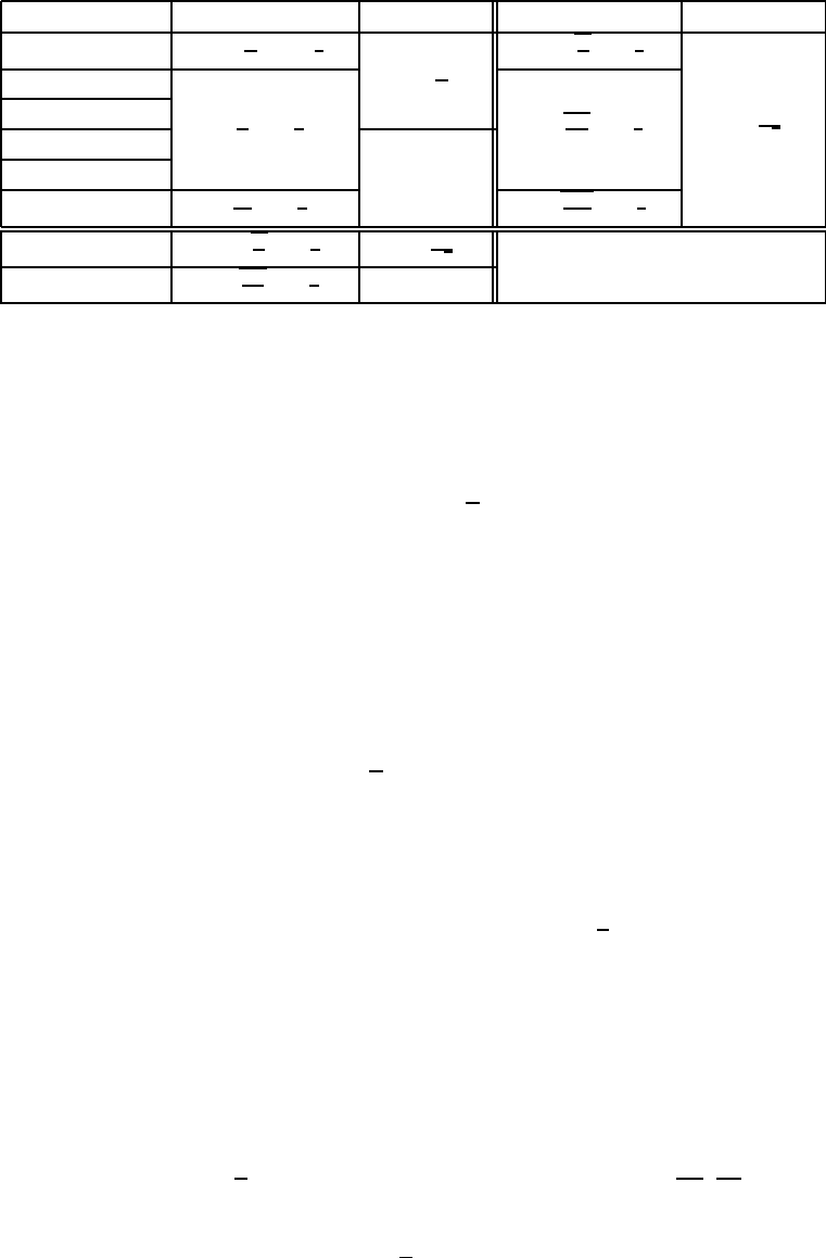
Comp. µ > 0 Comp. µ = 0 Catalyst µ > 0 Catalyst µ = 0

FG O





log













log









√



SAG [24]



log









log







SAGA [6]

Finito/MISO-Prox

not avail.

SDCA [25]

SVRG [27] O



′

log









′

log







Acc-FG [19] O



log









√



no acceleration

Acc-SDCA [26]

q

log







not avail.

Table 1: Comparison of rates of convergence, before and after the catalyst acceleration, resp. in

the strongly-convex and non strongly-convex cases. To simplify, we only present the case where

n ≤ L/µ when µ > 0. For all incremental algorithms, there is indeed no acceleration otherwise.

The quantity L

′

for SVRG is the average Lipschitz constant of the functions f

(see [27]).

inequalities. The current iterate x

is then obtained by minimizing the lower-bound of the objective

= arg min

x∈R

(

(x) =

i=1

(x)

)

. (13)

Interestingly, since D

is a lower-bound of F we also have D

) ≤ F

∗

, and thus the quantity

F (x

) − D

) can be used as an optimality certiﬁcate that upper-bounds F(x

) − F

∗

. Further-

more, this certiﬁcate was shown to convergeto zero with a rate similar to SAG/SDCA/SVRG/SAGA

under the condition n ≥ 2L/µ. In this section, we show how to remove this condition and how to

provide support to non-differentiable functions ψ whose proximal operator can be easily computed.

We shall brieﬂy sketch the main ideas, and we refer to Appendix D for a thorough presentation.

The ﬁrst idea to deal with a nonsmooth regularizer ψ is to change the deﬁnition of D

(x) =

i=1

(x) + ψ(x),

which was also proposed in [7] without a convergence proof. Then, because the d

’s are quadratic

functions, the minimizer x

of D

can be obtained by computing the proximal operator of ψ at a

particular point. The second idea to remove the condition n ≥ 2L/µ is to modify the update of the

lower bounds d

. Assume that index i

is selected among {1, . . . , n} at iteration k, then

(x) =



(1 − δ)d

k−1

(x)+ δ(f

k−1

)+h∇f

k−1

), x − x

k−1

kx − x

k−1

) if i = i

k−1

(x) otherwise

Whereas the original Finito/MISO uses δ = 1, our new variant uses δ = min(1, µn/2(L − µ)).

The resulting algorithm turns out to be very close to variant “5” of proximal SDCA [25], which

corresponds to using a different value for δ. The main difference between SDCA and MISO-

Prox is that the latter does not use duality. It also provides a different (simpler) optimality cer-

tiﬁcate F (x

) − D

), which is guaranteed to converge linearly, as stated in the next theorem.

Theorem 4.1 (Convergence of MISO-Prox).

Let (x

)

k≥0

be obtained by MISO-Prox, then

E[F (x

)] − F

∗

≤

(1 − τ)

k+1

(F (x

) − D

)) with τ ≥ min

. (14)

Furthermore, we also have fast convergence of the certiﬁcate

E[F (x

) − D

)] ≤

(1 − τ)

∗

− D

)) .

The proof of convergence is given in Appendix D. Finally, we conclude this section by noting that

MISO-Prox enjoys the catalyst acceleration, leading to the iteration-complexity presented in Ta-

ble 4.1. Since the convergence rate (14) does not have exactly the same form as (8), Propositions 3.2

and 3.4 cannot be used and additional analysis, given in Appendix D, is needed. Practical forms of

the algorithm are also presented there, along with discussions on how to initialize it.

5 Experiments

We evaluate the Catalyst acceleration on three methods that have never been accelerated in the past:

SAG [24], SAGA [6], and MISO-Prox. We focus on ℓ

-regularized logistic regression, where the

regularization parameter µ yields a lower bound on the strong convexity parameter of the problem.

We use three datasets used in [14], namely real-sim, rcv1, and ocr, which are relatively large, with

up to n = 2 500 000 points for ocr and p = 47 152 variables for rcv1. We consider three regimes:

µ = 0 (no regularization), µ/L = 0.001/n and µ/L = 0.1 /n, which leads signiﬁcantly larger

condition numbers than those used in other studies (µ/L ≈ 1/n in [14, 24]). We compare MISO,

SAG, and SAGA with their default parameters, which are recommended by their theoretical analysis

(step-sizes 1/L for SAG and 1/3L for SAGA), and study several accelerated variants. The values of

κ and ρ and the sequences (ε

)

k≥0

are those suggested in the previous sections, with η = 0.1 in (10).

Other implementation details are presented in Appendix E.

The restarting strategy for M is key to achieve acceleration in practice. All of the methods we com-

pare store n gradients evaluated at previous iterates of the algorithm. We always use the gradients

from the previous run of M to initialize a new one. We detail in Appendix E the initialization for

each method. Finally, we evaluated a heuristic that constrain M to always perform at most n iter-

ations (one pass over the data); we call this variant AMISO2 for MISO whereas AMISO1 refers to

the regular “vanilla” accelerated variant, and we also use this heuristic to accelerate SAG.

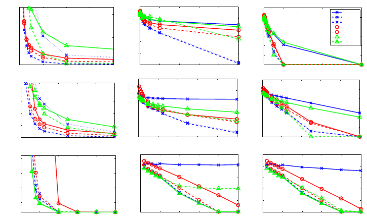
The results are reported in Table 1. We always obtain a huge speed-up for MISO, which suffers from

numerical stability issues when the condition number is very large (for instance, µ/L = 1 0

−3

/n =

4.10

−10

for ocr). Here, not only does the catalyst algorithm accelerate MISO, but it also stabilizes

it. Whereas MISO is slower than SAG and SAGA in this “small µ” regime, AMISO2 is almost

systematically the best performer. We are also able to accelerate SAG and SAGA in general, even

though the improvement is less signiﬁcant than for MISO. In particular, SAGA without acceleration

proves to be the best method on ocr. One reason may be its ability to adapt to the unknown strong

convexity parameter µ

′

≥ µ of the objective near the solution. When µ

′

/L ≥ 1/n, we indeed obtain

a regime where acceleration does not occur (see Sec. 4). Therefore, this experiment suggests that

adaptivity to unknown strong convexity is of high interest for incremental optimization.

0 50 100 150 200

x 10

−3

#Passes, Dataset real-sim, µ = 0

Objective function

0 100 200 300 400 500

−8

−6

−4

−2

#Passes, Dataset real-sim, µ/L = 10

−3

Relative duality gap

0 100 200 300 400 500

−10

−8

−6

−4

−2

#Passes, Dataset real-sim, µ/L = 10

−1

Relative duality gap

MISO

AMISO1

AMISO2

SAG

ASAG

SAGA

ASAGA

0 20 40 60 80 100

0.096

0.098

0.1

0.102

0.104

#Passes, Dataset rcv1, µ = 0

Objective function

0 20 40 60 80 100

−4

−2

#Passes, Dataset rcv1, µ/L = 10

−3

Relative duality gap

0 20 40 60 80 100

−10

−8

−6

−4

−2

#Passes, Dataset rcv1, µ/L = 10

−1

Relative duality gap

0 5 10 15 20 25

0.4957

0.4958

0.4959

0.496

#Passes, Dataset ocr, µ = 0

Objective function

0 5 10 15 20 25

−10

−8

−6

−4

−2

#Passes, Dataset ocr, µ/L = 10

−3

Relative duality gap

0 5 10 15 20 25

−10

−8

−6

−4

−2

#Passes, Dataset ocr, µ/L = 10

−1

Relative duality gap

Figure 1: Objective function value (or duality gap) for different number of passes performed over

each dataset. The legend for all curves is on the top right. AMISO, ASAGA, ASAG refer to the

accelerated variants of MISO, SAGA, and SAG, respectively.

Acknowledgments

This work was supported by ANR (MACARON ANR-14-CE23-0003-01), MSR-Inria joint centre,

CNRS-Mastodons program (Titan), and NYU Moore-Sloan Data Science Environment.

References

[1] A. Agarwal and L. Bottou. A lower bound for the optimization of ﬁnite sums. In Proc. International

Conference on Machine Learning (ICML), 2015.

[2] F. Bach, R. Jenatton, J. Mairal, and G. Obozinski. Optimization with sparsity-inducing penalties. Foun-

dations and Trends in Machine Learning, 4(1):1–106, 2012.

[3] H. H. Bauschke and P. L. Combettes. Convex Analysis and Monotone Operator Theory in Hilbert Spaces.

Springer, 2011.

[4] A. Beck and M. Teboulle. A fast iterative shrinkage-thresholding algorithm for linear inverse problems.

SIAM Journal on Imaging Sciences, 2(1):183–202, 2009.

[5] D. P. Bertsekas. Convex Optimization Algorithms. Athena Scientiﬁc, 2015.

[6] A. J. Defazio, F. Bach, and S. Lacoste-Julien. SAGA: A fast incremental gradient method with support

for non-strongly convex composite objectives. In Adv. Neural Information Processing Systems (NIPS),

2014.

[7] A. J. Defazio, T. S. Caetano, and J. Domke. Finito: A faster, permutable incremental gradient method for

big data problems. In Proc. International Conference on Machine Learning (ICML), 2014.

[8] R. Frostig, R. Ge, S. M. Kakade, and A. Sidford. Un-regularizing: approximate proximal point algorithms

for empirical risk minimization. In Proc. International Conference on Machine Learning (ICML), 2015.

[9] O. G¨uler. New proximal point algorithms for convex minimization. SIAM Journal on Optimization,

2(4):649–664, 1992.

[10] B. He and X. Yuan. An accelerated inexact proximal point algorithm for convex minimization. Journal

of Optimization Theory and Applications, 154(2):536–548, 2012.

[11] J.-B. Hiriart-Urruty and C. Lemar´echal. Convex Analysis and Minimization Algorithms I. Springer, 1996.

[12] A. Juditsky and A. Nemirovski. First order methods for nonsmooth convex large-scale optimization.

Optimization for Machine Learning, MIT Press, 2012.

[13] G. Lan. An optimal randomized incremental gradient method. arXiv:1507.02000, 2015.

[14] J. Mairal. Incremental majorization-minimization optimization with application to large-scale machine

learning. SIAM Journal on Optimization, 25(2):829–855, 2015.

[15] A. Nemirovski, A. Juditsky, G. Lan, and A. Shapiro. Robust stochastic approximation approach to

stochastic programming. SIAM Journal on Optimization, 19(4):1574–1609, 2009.

[16] Y. Nesterov. A method of solving a convex programming problem with convergence rate O(1/k

). Soviet

Mathematics Doklady, 27(2):372–376, 1983.

[17] Y. Nesterov. Introductory Lectures on Convex Optimization: A Basic Course. Springer, 2004.

[18] Y. Nesterov. Efﬁciency of coordinate descent methods on huge-scale optimization problems. SIAM

Journal on Optimization, 22(2):341–362, 2012.

[19] Y. Nesterov. Gradient methods for minimizing composite functions. Mathematical Programming,

140(1):125–161, 2013.

[20] N. Parikh and S.P. Boyd. Proximal algorithms. Foundations and Trends in Optimization, 1(3):123–231,

2014.

[21] P. Richt´arik and M. Tak´aˇc. Iteration complexity of randomized block-coordinate descent methods for

minimizing a composite function. Mathematical Programming, 144(1-2):1–38, 2014.

[22] S. Salzo and S. Villa. Inexact and accelerated proximal point algorithms. Journal of Convex Analysis,

19(4):1167–1192, 2012.

[23] M. Schmidt, N. Le Roux, and F. Bach. Convergence rates of inexact proximal-gradient methods for

convex optimization. In Adv. Neural Information Processing Systems (NIPS), 2011.

[24] M. Schmidt, N. Le Roux, and F. Bach. Minimizing ﬁnite sums with the stochastic average gradient.

arXiv:1309.2388, 2013.

[25] S. Shalev-Shwartz and T. Zhang. Proximal stochastic dual coordinate ascent. arXiv:1211.2717, 2012.

[26] S. Shalev-Shwartz and T. Zhang. Accelerated proximal stochastic dual coordinate ascent for regularized

loss minimization. Mathematical Programming, 2015.

[27] L. Xiao and T. Zhang. A proximal stochastic gradient method with progressive variance reduction. SIAM

Journal on Optimization, 24(4):2057–2075, 2014.

[28] Y. Zhang and L. Xiao. Stochastic primal-dual coordinate method for regularized empirical risk minimiza-

tion. In Proc. International Conference on Machine Learning (ICML), 2015.

In this appendix, Section A is devoted to the construction of an object called estimate sequence,

originally introduced by Nesterov (see [17]), and introduce extensions to deal with inexact mini-

mization. This section contains a generic convergence result that will be used to prove the main

theorems and propositions of the paper in Section B. Then, Section C is devoted to the computation

of global convergence rates of accelerated algorithms, Section D presents in details the proximal

MISO algorithm, and Section E gives some implementation details of the experiments.

A Construction of the Approximate Estimate Sequence

The estimate sequence is a generic tool introduced by Nesterov for proving the convergence of

accelerated gradient-based algorithms. We start by recalling the deﬁnition given in [17].

Deﬁnition A.1 (Estimate Sequence [17]).

A pair of sequences (ϕ

)

k≥0

and (λ

)

k≥0

, with λ

≥ 0 and ϕ

: R

→ R, is called an estimate

sequence of function F if

→ 0,

and for any x in R

and all k ≥ 0, we have

(x) ≤ (1 − λ

)F (x) + λ

(x).

Estimate sequences are used for proving convergence rates thanks to the following lemma

Lemma A.2 (Lemma 2.2.1 from [17]).

If for some sequence (x

)

k≥0

we have

F (x

) ≤ ϕ

∗

, min

x∈R

(x),

for an estimate sequence (ϕ

)

k≥0

of F , then

F (x

) − F

∗

≤ λ

(ϕ

∗

) − F

∗

where x

∗

is a minimizer of F .

The rate of convergence of F(x

) is thus directly related to the convergence rate of λ

. Constructing

estimate sequences is thus appealing, even though ﬁnding the most appropriate one is not trivial for

the catalyst algorithm because of the approximate minimization of G

in (5). In a nutshell, the main

steps of our convergence analysis are

1. deﬁne an “approximate” estimate sequence for F corresponding to Algorithm 1—that is,

ﬁnding a function ϕ that almost satisﬁes Deﬁnition A.1 up to the approximation errors ε

made in (5) when minimizing G

, and control the way these errors sum up together.

2. extend Lemma A.2 to deal with the approximationerrors ε

to derivea generic convergence

rate for the sequence (x

)

k≥0

This is also the strategy proposed by G¨uler in [9] for his inexact accelerated proximal point al-

gorithm, which essentially differs from ours in its stopping criterion. The estimate sequence we

choose is also different and leads to a more rigorous convergence proof. Speciﬁcally, we prove in

this section the following theorem:

Theorem A.3 (Convergence Result Derived from an Approximate Estimate Sequence).

Let us denote

k−1

i=0

(1 − α

), (15)

where the α

’s are deﬁned in Algorithm 1. Then, the sequence (x

)

k≥0

satisﬁes

F (x

) − F

∗

≤ λ

+ 2

i=1

, (16)

where F

∗

is the minimum value of F and

= F (x

) − F

∗

− x

∗

i=1

where γ

((κ + µ)α

− µ)

1 − α

, (17)

where x

∗

is a minimizer of F .

Then, the theorem will be used with the following lemma from [17] to control the convergence rate

of the sequence (λ

)

k≥0

, whose deﬁnition follows the classical use of estimate sequences [17]. This

will provide us convergence rates both for the strongly convex and non-strongly convex cases.

Lemma A.4 (Lemma 2.2.4 from [17]).

If in the quantity γ

deﬁned in (17) satisﬁes γ

≥ µ, then the sequence (λ

)

k≥0

from (15) satisﬁes

≤ min











(1 −

√



2 + k

κ+µ













. (18)

We may now move to the proof of the theorem.

A.1 Proof of Theorem A.3

The ﬁrst step is to construct an estimate sequence is typically to ﬁnd a sequence of lower bounds

of F . By calling x

∗

the minimizer of G

, the following one is used in [9]:

Lemma A.5 (Lower Bound for F near x

∗

For all x in R

F (x) ≥ F (x

∗

) + hκ(y

k−1

− x

∗

), x − x

∗

i +

kx − x

∗

. (19)

Proof. By strong convexity, G

(x) ≥ G

∗

) +

κ+µ

kx − x

∗

, which is equivalent to

F (x) +

kx − y

≥ F (x

∗

) +

∗

− y

k−1

κ + µ

kx − x

∗

After developing the quadratic terms, we directly obtain (19).

Unfortunately, the exact value x

∗

is unknown in practice and the estimate sequence of [9] yields

in fact an algorithm where the deﬁnition of the anchor point y

involves the unknown quantity x

∗

instead of the approximate solutions x

and x

k−1

as in (6), as also noted by others [22]. To obtain a

rigorous proof of convergence for Algorithm 1, it is thus necessary to reﬁne the analysis of [9]. To

that effect, we construct below a sequence of functions that approximately satisﬁes the deﬁnition of

estimate sequences. Essentially, we replace in (19) the quantity x

∗

by x

to obtain an approximate

lower bound, and control the error by using the condition G

) − G

∗

) ≤ ε

. This leads us to

the following construction:

1. φ

(x) = F (x

) +

kx − x

;

2. For k ≥ 1, we set

(x) = (1 − α

k−1

)φ

k−1

(x) + α

k−1

[F (x

) + hκ(y

k−1

− x

), x − x

i +

kx − x

where the value of γ

, given in (17) will be explained later. Note that if one replaces x

by x

∗

the above construction, it is easy to show that (φ

)

k≥0

would be exactly an estimate sequence for F

with the relation λ

given in (15).

Before extending Lemma A.2 to deal with the approximate sequence and conclude the proof of

the theorem, we need to characterize a few properties of the sequence (φ

)

k≥0

. In particular, the

functions φ

are quadratic and admit a canonical form:

Lemma A.6 (Canonical Form of the Functions φ

For all k ≥ 0, φ

can be written in the canonical form

(x) = φ

∗

kx − v

where the sequences (γ

)

k≥0

, (v

)

k≥0

, and (φ

∗

)

k≥0

are deﬁned as follows

= (1 − α

k−1

)γ

k−1

+ α

k−1

µ, (20)

((1 − α

k−1

)γ

k−1

+ α

k−1

µx

− α

k−1

κ(y

k−1

− x

)) , (21)

∗

= (1 − α

k−1

)φ

∗

k−1

+ α

k−1

F (x

) −

k−1

2γ

kκ(y

k−1

− x

k−1

(1 − α

k−1

)γ

k−1



− v

k−1

+ hκ(y

k−1

− x

), v

k−1

− x



, (22)

Proof. We have for all k ≥ 1 and all x in R

(x) = (1 − α

k−1

)



∗

k−1

kx − v

k−1



+ α

k−1



F (x

) + hκ(y

k−1

− x

), x − x

i +

kx − x



= φ

∗

kx − v

(23)

Differentiate twice the relations (23) gives us directly (20). Since v

minimizes φ

, the optimality

condition ∇φ

) = 0 gives

(1 − α

k−1

)γ

k−1

− v

k−1

) + α

k−1

(κ(y

k−1

− x

) + µ(v

− x

)) = 0,

and then we obtain (21). Finally, apply x = x

to (23), which yields

) = (1 − α

k−1

)



∗

k−1

− v

k−1



+ α

k−1

F (x

) = φ

∗

− v

Consequently,

∗

= (1 − α

k−1

)φ

∗

k−1

+ α

k−1

F (x

) + (1 − α

k−1

)

k−1

− v

k−1

−

− v

(24)

Using the expression of v

from (21), we have

− x

((1 − α

k−1

)γ

k−1

− x

) − α

k−1

κ(y

k−1

− x

)) .

Therefore

− v

(1 − α

k−1

)

k−1

2γ

− v

k−1

−

(1 − α

k−1

)α

k−1

− x

, κ(y

k−1

− x

)i +

k−1

2γ

kκ(y

k−1

− x

It remains to plug this relation into (24), use once (20), and we obtain the formula (22) for φ

∗

We may now start analyzing the errors ε

to control how far is the sequence (φ

)

k≥0

from an exact

estimate sequence. For that, we need to understand the effect of replacing x

∗

by x

in the lower

bound (19). The following lemma will be useful for that purpose.

Lemma A.7 (Controlling the Approximate Lower Bound of F ).

If G

) − G

∗

) ≤ ε

, then for all x in R

F (x) ≥ F (x

) + hκ(y

k−1

−x

), x −x

kx −x

+ (κ + µ)hx

−x

∗

, x − x

i− ε

. (25)

Proof. By strong convexity, for all x in R

(x) ≥ G

∗

κ + µ

kx − x

∗

where G

∗

is the minimum value of G

. Replacing G

by its deﬁnition (5) gives

F (x) ≥ G

∗

κ + µ

kx − x

∗

−

kx − y

k−1

= G

) + (G

∗

− G

)) +

κ + µ

kx − x

∗

−

kx − y

k−1

≥ G

) − ε

κ + µ

k(x − x

) + (x

− x

∗

−

kx − y

k−1

≥ G

) − ε

κ + µ

kx − x

−

kx − y

k−1

+ (κ + µ)hx

− x

∗

, x − x

We conclude by noting that

kx − x

−

kx − y

k−1

=F (x

− y

k−1

kx − x

−

kx − y

k−1

= F (x

) + hκ(y

k−1

− x

), x − x

We can now show that Algorithm 1 generates iterates (x

)

k≥0

that approximately satisfy the condi-

tion of Lemma A.2 from Nesterov [17].

Lemma A.8 (Relation between (φ

)

k≥0

and Algorithm 1).

Let φ

be the estimate sequence constructed above. Then, Algorithm 1 generates iterates (x

)

k≥0

such that

F (x

) ≤ φ

∗

+ ξ

where the sequence (ξ

)

k≥0

is deﬁned by ξ

= 0 and

= (1 − α

k−1

)(ξ

k−1

+ ε

− (κ + µ)hx

− x

∗

, x

k−1

− x

i).

Proof. We proceed by induction. For k = 0, φ

∗

= F (x

) and ξ

= 0.

Assume now that F (x

k−1

) ≤ φ

∗

k−1

+ ξ

k−1

. Then,

∗

k−1

≥ F (x

k−1

) − ξ

k−1

≥ F (x

) + hκ(y

k−1

− x

), x

k−1

− x

i + (κ + µ)hx

− x

∗

, x

k−1

− x

i − ε

− ξ

k−1

= F (x

) + hκ(y

k−1

− x

), x

k−1

− x

i − ξ

/(1 − α

k−1

where the second inequality is due to (25). By Lemma A.6, we now have,

∗

= (1 − α

k−1

)φ

∗

k−1

+ α

k−1

F (x

) −

k−1

2γ

kκ(y

k−1

− x

k−1

(1 − α

k−1

)γ

k−1



− v

k−1

+ hκ(y

k−1

− x

), v

k−1

− x



≥ (1 − α

k−1

) (F (x

) + hκ(y

k−1

− x

), x

k−1

− x

i) − ξ

+ α

k−1

F (x

)

−

k−1

2γ

kκ(y

k−1

− x

k−1

(1 − α

k−1

)γ

k−1

hκ(y

k−1

− x

), v

k−1

− x

= F (x

) + (1 − α

k−1

)hκ(y

k−1

− x

), x

k−1

− x

k−1

− x

−

k−1

2γ

kκ(y

k−1

− x

− ξ

= F (x

) + (1 − α

k−1

)hκ(y

k−1

− x

), x

k−1

− y

k−1

− y

k−1



1 −

(κ + 2µ)α

k−1

2γ



κk(y

k−1

− x

− ξ

We now need to show that the choice of the sequences (α

)

k≥0

and (y

)

k≥0

will cancel all the terms

involving y

k−1

− x

. In other words, we want to show that

k−1

− y

k−1

− y

k−1

) = 0, (26)

and we want to show that

1 − (κ + µ)

k−1

= 0, (27)

which will be sufﬁcient to conclude that φ

∗

+ ξ

≥ F (x

). The relation (27) can be obtained from

the deﬁnition of α

in (6) and the form of γ

given in (20). We have indeed from (6) that

(κ + µ)α

= (1 − α

)(κ + µ)α

k−1

+ α

µ.

Then, the quantity (κ + µ)α

follows the same recursion as γ

k+1

in (20). Moreover, we have

= (1 − α

)γ

+ µα

= (κ + µ)α

from the deﬁnition of γ

in (17). We can then conclude by induction that γ

k+1

= (κ + µ)α

for

all k ≥ 0 and (27) is satisﬁed.

To prove(26), we assume that y

k−1

is chosen such that (26) is satisﬁed, and show that it is equivalent

to deﬁning y

as in (6). By lemma A.6,

((1 − α

k−1

)γ

k−1

+ α

k−1

µx

− α

k−1

κ(y

k−1

− x

))



(1 − α

k−1

)

k−1

((γ

+ α

k−1

− γ

k−1

) + α

k−1

µx

− α

k−1

κ(y

k−1

− x

)





(1 − α

k−1

)

k−1

((γ

k−1

+ α

k−1

µ)y

k−1

− γ

k−1

) + α

k−1

(µ + κ)x

− α

k−1

κy

k−1





k−1

(γ

− µα

k−1

−

(1 − α

k−1

)

k−1

− α

k−1

κy

k−1



k−1

− (1 − α

k−1

), (28)

As a result, using (26) by replacing k − 1 by k yields

= x

k−1

(1 − α

k−1

)

k−1

+ α

− x

k−1

and we obtain the original equivalent deﬁnition of (6). This concludes the proof.

With this lemma in hand, we introduce the following proposition, which brings us almost to Theo-

rem A.3, which we want to prove.

Proposition A.9 (Auxiliary Proposition for Theorem A.3).

Let us consider the sequence (λ

)

k≥0

deﬁned in (15). Then, the sequence (x

)

k≥0

satisﬁes

(F (x

) − F

∗

− v

) ≤ φ

∗

) − F

∗

i=1

√

2ε

∗

− v

where x

∗

is a minimizer of F and F

∗

its minimum value.

Proof. By the deﬁnition of the function φ

, we have

∗

) = (1 − α

k−1

)φ

k−1

∗

) + α

k−1

[F (x

) + hκ(y

k−1

− x

), x

∗

− x

i +

∗

− x

]

≤ (1 − α

k−1

)φ

k−1

∗

) + α

k−1

[F (x

∗

) + ε

− (κ + µ)hx

− x

∗

, x

∗

− x

i],

where the inequality comes from (25). Therefore, by using the deﬁnition of ξ

in Lemma A.8,

∗

) + ξ

− F

∗

≤ (1 − α

k−1

)(φ

k−1

∗

) + ξ

k−1

− F

∗

) + ε

− (κ + µ)hx

− x

∗

, (1 − α

k−1

+ α

k−1

∗

− x

= (1 − α

k−1

)(φ

k−1

∗

) + ξ

k−1

− F

∗

) + ε

− α

k−1

(κ + µ)hx

− x

∗

, x

∗

− v

≤ (1 − α

k−1

)(φ

k−1

∗

) + ξ

k−1

− F

∗

) + ε

+ α

k−1

(κ + µ)kx

− x

∗

kkx

∗

− v

≤ (1 − α

k−1

)(φ

k−1

∗

) + ξ

k−1

− F

∗

) + ε

+ α

k−1

2(κ + µ)ε

∗

− v

= (1 − α

k−1

)(φ

k−1

∗

) + ξ

k−1

− F

∗

) + ε

2ε

∗

− v

where the ﬁrst equality uses the relation (28), the last inequality comes from the strong convex-

ity relation ε

≥ G

) − G

∗

) ≥ (1/2)(κ + µ)kx

∗

− x

, and the last equality uses the

relation γ

= (κ + µ)α

k−1

Dividing both sides by λ

yields

(φ

∗

) + ξ

− F

∗

) ≤

k−1

(φ

k−1

∗

) + ξ

k−1

− F

∗

) +

√

2ε

∗

− v

A simple recurrence gives,

(φ

∗

) + ξ

− F

∗

) ≤ φ

∗

) − F

∗

i=1

√

2ε

∗

− v

Finally, by lemmas A.6 and A.8,

∗

) + ξ

− F

∗

− v

+ φ

∗

+ ξ

− F

∗

≥

∗

− v

+ F (x

) − F

∗

As a result,

(F (x

) − F

∗

− v

) ≤ φ

∗

) − F

∗

i=1

√

2ε

∗

− v

k. (29)

To control the error term on the right and ﬁnish the proof of Theorem A.3, we are going to bor-

row some methodology used to analyze the convergence of inexact proximal gradient algorithms

from [23], and use an extension of a lemma presented in [23] to bound the value of kv

−x

∗

k. This

lemma is presented below.

Lemma A.10 (Simple Lemma on Non-Negative Sequences).

Assume that the nonnegative sequences (u

)

k≥0

and (a

)

k≥0

satisfy the following recursion for all

k ≥ 0:

≤ S

i=1

, (30)

where (S

)

k≥0

is an increasing sequence such that S

≥ u

. Then,

≤

i=1



i=1



+ S

. (31)

Moreover,

i=1

≤

i=1

Proof. The ﬁrst part—that is, Eq. (31)—is exactly Lemma 1 from [23]. The proof is in their ap-

pendix. Then, by calling b

the right-hand side of (31), we have that for all k ≥ 1, u

≤ b

Furthermore (b

)

k≥0

is increasing and we have

i=1

≤ S

i=1

≤ S



i=1



= b

and using the inequality

√

x + y ≤

√

x +

√

y, we have

i=1



i=1



+ S

≤

i=1



i=1



i=1

As a result,

i=1

≤ b

≤

i=1

We are now in shape to conclude the proof of Theorem A.3. We apply the previous lemma to (29):



∗

− v

+ F (x

) − F

∗



≤ φ

∗

) − F

∗

i=1

√

2ε

∗

− v

Since F (x

) − F

∗

≥ 0, we have

2λ

∗

− v

{z }

≤ φ

∗

) − F

∗

i=1

{z }

i=1

√

2ε

∗

− v

{z }

with

2λ

∗

− v

k and a

= 2

and S

= φ

∗

) − F

∗

i=1

Then by Lemma A.10, we have

F (x

) − F

∗

≤ λ

i=1

≤ λ

i=1

= λ

+ 2

i=1

which is the desired result.

B Proofs of the Main Theorems and Propositions

B.1 Proof of Theorem 3.1

Proof. We simply use Theorem A.3 and specialize it to the choice of parameters. The initialization

√

q leads to a particularly simple form of the algorithm, where α

√

q for all k ≥ 0.

Therefore, the sequence (λ

)

k≥0

from Theorem A.3 is also simple. For all k ≥ 0, we indeed have

= (1 −

√

. To upper-bound the quantity S

from Theorem A.3, we now remark that γ

= µ

and thus, by strong convexity of F ,

F (x

) +

− x

∗

− F

∗

≤ 2(F (x

) − F

∗

Therefore,

+ 2

i=1

F (x

) +

− x

∗

− F

∗

i=1

+ 2

i=1

≤

F (x

) +

− x

∗

− F

∗

+ 3

i=1

≤

2(F (x

) − F

∗

) + 3

i=1

2(F (x

) − F

∗

)







1 +

i=1

1 − ρ

1 −

√

{z }







2(F (x

) − F

∗

)

k+1

− 1

η −1

≤

2(F (x

) − F

∗

)

k+1

η − 1

Therefore, Theorem A.3 combined with the previous inequality gives us

F (x

) − F

∗

≤ 2λ

(F (x

) − F

∗

)



k+1

η − 1



= 2



η −1



(1 − ρ)

(F (x

) − F

∗

)

= 2

√

1 − ρ

√

1 − ρ −

1 −

√

(1 − ρ)

(F (x

) − F

∗

)

= 2

√

1 − ρ −

1 −

√

(1 − ρ)

k+1

(F (x

) − F

∗

Since

√

1 − x +

is decreasing in [0, 1], we have

√

1 − ρ +

≥

1 −

√

q +

√

. Consequently,

F (x

) − F

∗

≤

(

√

q −ρ)

(1 − ρ)

k+1

(F (x

) − F

∗

B.2 Proof of Proposition 3.2

To control the number of calls of M, we need to upper bound G

k−1

) − G

∗

which is given by

the following lemma:

Lemma B.1 (Relation between G

k−1

) and ε

k−1

Let (x

)

k≥0

and (y

)

k≥0

be generated by Algorithm 1. Remember that by deﬁnition of x

k−1

) − G

∗

k−1

≤ ε

k−1

Then, we have

k−1

) − G

∗

≤ 2ε

k−1

κ + µ

k−1

− y

k−2

. (32)

Proof. We ﬁrst remark that for any x, y in R

, we have

(x) − G

k−1

(x) = G

(y) − G

k−1

(y) + κhy − x, y

k−1

− y

k−2

i, ∀k ≥ 2,

which can be shown by using the respective deﬁnitions of G

and G

k−1

and manipulate the quadratic

term resulting from the difference G

(x) − G

k−1

(x).

Plugging x = x

k−1

and y = x

∗

in the previous relation yields

k−1

) − G

∗

= G

k−1

) − G

k−1

∗

) + κhx

∗

− x

k−1

, y

k−1

− y

k−2

= G

k−1

) − G

∗

k−1

+ G

∗

k−1

− G

k−1

∗

) + κhx

∗

− x

k−1

, y

k−1

− y

k−2

≤ ε

k−1

+ G

∗

k−1

− G

k−1

∗

) + κhx

∗

− x

k−1

, y

k−1

− y

k−2

≤ ε

k−1

−

µ + κ

∗

− x

∗

k−1

+ κhx

∗

− x

k−1

, y

k−1

− y

k−2

(33)

where the last inequality comes from the strong convexity inequality of

k−1

∗

) ≥ G

∗

k−1

µ + κ

∗

− x

∗

k−1

Moreover, from the inequality hx, yi ≤

kxk

kyk

, we also have

κhx

∗

− x

∗

k−1

, y

k−1

− y

k−2

i ≤

µ + κ

∗

− x

∗

k−1

2(κ + µ)

k−1

− y

k−2

, (34)

and

κhx

∗

k−1

− x

k−1

, y

k−1

− y

k−2

i ≤

µ + κ

∗

k−1

− x

k−1

2(κ + µ)

k−1

− y

k−2

≤ ε

k−1

2(κ + µ)

k−1

− y

k−2

(35)

Summing inequalities (33), (34) and (35) gives the desired result.

Next, we need to upper-boundthe term ky

k−1

−y

k−2

, which was also required in the convergence

proof of the accelerated SDCA algorithm [26]. We follow here their methodology.

Lemma B.2 (Control of the term ky

k−1

− y

k−2

.).

Let us consider the iterates (x

)

k≥0

and (y

)

k≥0

produced by Algorithm 1, and deﬁne

= C(1 − ρ)

k+1

(F (x

) − F

∗

which appears in Theorem 3.1 and which is such that F (x

) − F

∗

≤ δ

. Then, for any k ≥ 3 ,

k−1

− y

k−2

≤

k−3

Proof. We follow here [26]. By deﬁnition of y

, we have

k−1

− y

k−2

k = kx

k−1

+ β

k−1

− x

k−2

) − x

k−2

− β

k−2

− x

k−3

≤ (1 + β

k−1

)kx

k−1

− x

k−2

k + β

k−2

− x

k−3

≤ 3 max {kx

k−1

− x

k−2

k, kx

k−2

− x

k−3

k},

where β

is deﬁned in (6). The last inequality was due to the fact that β

≤ 1. Indeed, the speciﬁc

choice of α

√

q in Theorem A.3 leads to β

√

q−q

√

q+q

≤ 1 for all k. Note, however, that this

relation β

≤ 1 is true regardless of the choice of α



k−1

− α

k−1





k−1

+ α



k−1

+ α

k−1

− 2α

k−1

+ 2α

k−1

+ α

k−1

+ α

k−1

− 2α

k−1

+ α

k−1

+ qα

+ α

k−1

≤ 1,

where the last equality uses the relation α

+α

k−1

= α

k−1

+qα

from Algorithm 1. To conclude

the lemma, we notice that by triangle inequality

− x

k−1

k ≤ kx

− x

∗

k + kx

k−1

− x

∗

and by strong convexity of F

− x

∗

≤ F (x

) − F (x

∗

) ≤ δ

As a result,

k−1

− y

k−2

≤ 9 max



k−1

− x

k−2

, kx

k−2

− x

k−3



≤ 36 ma x



k−1

− x

∗

, kx

k−2

− x

∗

, kx

k−3

− x

∗



≤

k−3

We are now in shape to conclude the proof of Proposition 3.2.

By Proposition B.1 and lemma B.2, we have for all k ≥ 3,

k−1

) − G

∗

≤ 2ε

k−1

κ + µ

k−3

≤ 2ε

k−1

72κ

k−3

Let (z

)

t≥0

be the sequence of using M to solve G

with initialization z

= x

k−1

. By assump-

tion (8), we have

) − G

∗

≤ A (1 − τ

)

k−1

) − G

∗

) ≤ A e

−τ

k−1

) − G

∗

The number of iterations T

of M to guarantee an accuracy of ε

needs to satisfy

A e

−τ

k−1

) − G

∗

) ≤ ε

which gives



log



A(G

k−1

) − G

∗

)



. (36)

Then, it remains to upper-bound

k−1

) − G

∗

≤

2ε

k−1

72κ

k−3

2(1 − ρ) +

72κ

(1 − ρ)

1 − ρ

2592κ

µ(1 − ρ)

(

√

q − ρ)

Let us denote R the right-hand side. We remark that this upper bound holds for k ≥ 3. We now

consider the cases k = 1 and k = 2.

When k = 1, G

(x) = F (x) +

kx −y

. Note that x

= y

, then G

) = F (x

). As a result,

) − G

∗

= F (x

) − F (x

∗

) −

∗

− y

≤ F (x

) − F (x

∗

) ≤ F (x

) − F

∗

Therefore,

) − G

∗

≤

F (x

) − F

∗

2(1 − ρ)

≤ R.

When k = 2, we remark that y

− y

= (1 + β

)(x

− x

). Then, by following similar steps as in

the proof of Lemma B.2, we have

− y

≤ 4kx

− x

≤

32δ

which is smaller than

72δ

−1

. Therefore, the previous steps from the case k ≥ 3 apply and

)−G

∗

≤ R. Thus, for any k ≥ 1,

≤



log (AR)



, (37)

which concludes the proof.

B.3 Proof of Theorem 3.3.

We will again Theorem A.3 and specialize it to the choice of parameters. To apply it, the following

Lemma will be useful to control the growth of (λ

)

k≥0

Lemma B.3 (Growth of the Sequence (λ

)

k≥0

Let (λ

)

k≥0

be the sequence deﬁned in (15) where (α

)

k≥0

is produced by Algorithm 1 with α

√

5−1

and µ = 0. Then, we have the following bounds for all k ≥ 0,

(k + 2)

≥ λ

≥

(k + 2)

Proof. Note that by deﬁnition of α

, we have for all k ≥ 1,

= (1 − α

)α

k−1

i=1

(1 − α

)α

= λ

k+1

1 − α

= λ

k+1

With the choice of α

, the quantity γ

deﬁned in (17) is equal to κ. By Lemma A.4, we have

≤

(k+2)

for all k ≥ 0 and thus α

≤

k+3

for all k ≥ 1 (it is also easy to check numerically

that this is also true for k = 0 since

√

5−1

≈ 0.62 ≤

). We now have all we need to conclude the

lemma:

k−1

i=0

(1 − α

) ≥

k−1

i=0



1 −

i + 3



(k + 2)(k + 1)

≥

(k + 2)

With this lemma in hand, we may now proceed and apply Theorem A.3. We have remarked in the

proof of the previous lemma that γ

= κ. Then,

+ 2

i=1

F (x

) − F

∗

− x

∗

i=1

+ 2

i=1

≤

F (x

) − F

∗

− x

∗

+ 3

i=1

≤

− x

∗

F (x

) − F

∗

1 +

i=1

(i + 2)

1+η/2

where the last inequality uses Lemma B.3 to upper-bound the ratio ε

/λ

. Moreover,

i=1

(i + 2)

1+η/2

≤

∞

i=2

1+η/2

≤

∞

1+η/2

dx =

Therefore, by (16) from Theorem A.3,

F (x

) − F

∗

≤ λ

+ 2

i=1

≤

(k + 2)



F (x

) − F

∗



1 +



− x

∗



≤

(k + 2)



1 +



(F (x

) − F

∗

) +

− x

∗

The last inequality uses (a + b)

≤ 2(a

+ b

B.4 Proof of Proposition 3.4

When µ = 0, we remark that Proposition B.1 still holds but Lemma B.2 does not. The main difﬁculty

is thus to ﬁnd another way to control the quantity ky

k−1

− y

k−2

Since F (x

) − F

∗

is bounded by Theorem 3.3, we may use the bounded level set assumptions to

ensure that there exists B > 0 such that kx

− x

∗

k ≤ B for any k ≥ 0 where x

∗

is a minimizer

of F . We can now follow similar steps as in the proof of Lemma B.2, and show that

k−1

− y

k−2

≤ 36B

Then by Proposition B.1,

k−1

) − G

∗

≤ 2ε

k−1

+ 36κB

Since κ > 0, G

is strongly convex, then using the same argument as in the strongly convex case,

the number of calls for M is given by



log



A(G

k−1

) − G

∗

)



. (38)

Again, we need to upper bound it

k−1

) − G

∗

≤

2ε

k−1

+ 36κB

2(k + 1)

4+η

(k + 2)

4+η

162κB

(k + 2)

4+η

(F (x

) − F

∗

)

The right hand side is upper-bounded by O((k + 2)

4+η

). Plugging this relation into (38) gives the

desired result.

C Derivation of Global Convergence Rates

We give here a generic “template” for computing the optimal choice of κ to accelerate a given

algorithm M, and therefore compute the rate of convergence of the accelerated algorithm A.

We assume here that M is a randomized ﬁrst-order optimization algorithm, i.e. the iterates (x

)

generated by M are a sequence of random variables; specialization to a deterministic algorithm is

straightforward. Also, for the sake of simplicity, we shall use simple notations to denote the stopping

time to reach accuracy ε. Deﬁnition and notation using ﬁltrations, σ-algebras, etc. are unnecessary

for our purpose here where the quantity of interest has a clear interpretation.

Assume that algorithm M enjoys a linear rate of convergence, in expectation. There exists con-

stants C

M,F

and τ

M,F

such that the sequence of iterates (x

)

k≥0

for minimizing a strongly-convex

objective F satisﬁes

E [F (x

) − F

∗

] ≤ C

M,F

(1 − τ

M,F

)

. (39)

Deﬁne the random variable T

M,F

(ε) (stopping time) corresponding to the minimum number of

iterations to guarantee an accuracy ε in the course of running M

M,F

(ε) := inf {k ≥ 1, F (x

) − F

∗

≤ ε} (40)

Then, an upper bound on the expectation is provided by the following lemma.

Lemma C.1 (Upper Bound on the expectation of T

M,F

(ε)).

Let M be an optimization method with the expected rate of convergence (39). Then,

E[T

(ε)] ≤

log



· ε



+ 1 =



log





, (41)

where we have dropped the dependency in F to simplify the notation.

Proof. We abbreviate τ

by τ. Set

log



1 − e

−τ



For any k ≥ 0, we have

E[F (x

) − F

∗

] ≤ C

(1 − τ)

≤ C

−kτ

By Markov’s inequality,

P[F (x

) − F

∗

> ε] = P[T

(ε) > k] ≤

E[F (x

) − F

∗

]

≤

−kτ

. (42)

Together with the fact P ≤ 1 and k ≥ 0. We have

P[T

(ε) ≥ k + 1] ≤ min



−kτ

, 1



Therefore,

E[T

(ε)] =

∞

k=1

P[T

(ε) ≥ k] =

k=1

P[T

(ε) ≥ k] +

∞

k=T

P[T

(ε) ≥ k]

≤ T

∞

k=T

−kτ

= T

−T

∞

k=0

−kτ

= T

−τ T

1 − e

−τ

= T

+ 1.

As simple calculation shows that for any τ ∈ (0, 1),

≤ 1 − e

−τ

and then

E[T

(ε)] ≤ T

+ 1 =

log



1 − e

−τ



+ 1 ≤

log



τε



+ 1.

Note that the previous lemma mirrors Eq. (36-37) in the proof of Prop. 3.1 in Appendix B. For all

optimization methods of interest, the rate τ

M,G

is independentof k and varies with the parameter κ.

We may now compute the iteration-complexity(in expectation) of the accelerated algorithm A—that

is, for a given ε, the expected total number of iterations performed by the method M. Let us now

ﬁx ε > 0. Calculating the iteration-complexity decomposes into three steps:

1. Find κ that maximizes the ratio τ

M,G

√

µ + κ for algorithm M when F is µ-strongly

convex. In the non-strongly convex case, we suggest maximizing instead the ratio

M,G

√

L + κ. Note that the choice of κ is less critical for non-strongly convex prob-

lems since it only affects multiplicative constants in the global convergence rate.

2. Compute the upper-bound of the number of outer iterations k

out

using Theorem 3.1 (for the

strongly convex case), or Theorem 3.3 (for the non-strongly convex case), by replacing κ

by the optimal value found in step 1.

3. Compute the upper-bound of the expected number of inner iterations

max

k=1,...,k

out

E[T

M,G

(ε

)] ≤ k

by replacing the appropriate quantities in Eq. 41 for algorithm M; for that purpose, the

proofs of Propositions 3.2 of 3.4 my be used to upper-bound the ratio C

M,G

/ε

, or another

dedicated analysis for M may be required if the constant C

M,G

does not have the required

form A(G

) − G

∗

) in (8).

Then, the iteration-complexity (in expectation) denoted Comp. is given by

Comp ≤ k

× k

out

. (43)

D A Proximal MISO/Finito Algorithm

In this section, we present the algorithm MISO/Finito, and show how to extend it in two ways. First,

we propose a proximal version to deal with composite optimization problems, and we analyze its

rate of convergence. Second, we show how to remove a large sample condition n ≥ 2L/µ, which

was necessary for the convergence of the algorithm. The resulting algorithm is a variant of proximal

SDCA [25] with a different stepsize and a stopping criterion that does not use duality.

D.1 The Original Algorithm MISO/Finito

MISO/Finito was proposed in [14] and [7] for solving the following smooth unconstrained convex

minimization problem

min

x∈R

(

f(x) ,

i=1

(x)

)

, (44)

where each f

is differentiable with L-Lipschitz continuous derivatives and µ-strongly convex. At

iteration k, the algorithm updates a list of lower bounds d

of the functions f

, by randomly picking

up one index i

among {1, ··· , n} and performing the following update

(x) =



k−1

) + h∇f

k−1

), x − x

k−1

i +

kx − x

k−1

if i = i

k−1

(x) otherwise

which is a lower bound of f

because of the µ-strong convexity of f

. Equivalently, one may perform

the following updates



k−1

−

∇f

k−1

) if i = i

k−1

otherwise

and all functions d

have the form

(x) = c

kx − z

where c

is a constant. Then, MISO/Finito performs the following minimization to produce the

iterate (x

= arg min

x∈R

i=1

(x) =

i=1

which is equivalent to

← x

k−1

−



− z

k−1



In many machine learning problems, it is worth remarking that each function f

(x) has the spe-

ciﬁc form f

(x) = l

(hx, w

i) +

kxk

. In such cases, the vectors z

can be obtained by storing

only O(n) scalars.

The main convergence result of [14] is that the procedure above converges with

a linear rate of convergence of the form (3), with τ

MISO

= 1/3n (also reﬁned in 1/2n in [7]), when

the large sample size constraint n ≥ 2L/µ is satisﬁed.

Removing this condition and extending MISO to the composite optimization problem (1) is the

purpose of the next section.

D.2 Proximal MISO

We now consider the composite optimization problem below,

min

x∈R

(

F (x) =

i=1

(x) + ψ(x)

)

where the functions f

are differentiable with L-Lipschitz derivatives and µ-strongly convex. As in

typical composite optimization problems, ψ is convex but not necessarily differentiable. We assume

that the proximal operator of ψ can be computed easily. The algorithm needs to be initialized with

some lower bounds for the functions f

(x) ≥

kx − z

+ c

, (A1)

which are guaranteed to exist due to the µ-strong convexity of f

. For typical machine learning

applications, such initialization is easy. For example, logistic regression with ℓ

-regularization sat-

isﬁes (A1) with z

= 0 and c

= 0. Then, the MISO-Prox scheme is given in Algorithm 2. Note

that if no simple initialization is available, we may consider any initial estimate ¯z

in R

and deﬁne

= ¯z

− (1/µ)∇f

(¯z

), which requires performing one pass over the data.

Then, we remark that under the large sample size condition n ≥ 2L/µ, we have δ = 1 and the

update of the quantities z

in (45) is the same as in the original MISO/Finito algorithm. As we will

see in the convergence analysis, the choice of δ ensures convergence of the algorithm even in the

small sample size regime n < 2L/µ.

Relation with Proximal SDCA [25]. The algorithm MISO-Prox is almost identical to variant 5

of proximal SDCA [25], which performs the same updates with δ = µn/(L + µn) instead of δ =

min(1,

µn

2(L−µ)

). It is however not clear that MISO-Prox actually performs dual ascent steps in the

sense of SDCA since the proof of convergence of SDCA cannot be directly modiﬁed to use the

stepsize of proximal MISO and furthermore, the convergence proof of MISO-Prox does not use the

concept of duality. Another difference lies in the optimality certiﬁcate of the algorithms. Whereas

Proximal-SDCA provides a certiﬁcate in terms of linear convergence of a duality gap based on

Fenchel duality, Proximal-SDCA ensures linear convergence of a gap that relies on strong convexity

but not on the Fenchel dual (at least explicitly).

Optimality Certiﬁcate and Stopping Criterion. Similar to the original MISO algorithm, Prox-

imal MISO maintains a list (d

) of lower bounds of the functions f

, which are updated in the

following fashion

(x) =



(1 − δ)d

k−1

(x)+ δ



k−1

)+h∇f

k−1

), x − x

k−1

kx − x

k−1



if i = i

k−1

(x) otherwise

(46)

Note that even though we call this algorithm MISO (or Finito), it was called MISOµ in [14], whereas

“MISO” was originally referring to an incremental majorization-minimization procedure that uses upper bounds

of the functions f

instead of lower bounds, which is appropriate for non-convex optimization problems.

Algorithm 2 MISO-Prox: an improved MISO algorithm with proximal support.

input (z

)

i=1,...,n

such that (A1) holds; N (number of iterations);

1: initialize ¯z

i=1

and x

= prox

ψ/µ

[¯z

];

2: deﬁne δ = min



µn

2(L−µ)



;

3: for k = 1, . . . , N do

4: randomly pick up an index i

in {1, . . . , n};

5: update

(

(1 − δ)z

k−1

+ δ



k−1

−

∇f

k−1

)



if i = i

k−1

otherwise

¯z

= ¯z

k−1

−



− z

k−1



i=1

= prox

ψ/µ

[¯z

(45)

6: end for

output x

(ﬁnal estimate).

Then, the following function is a lower bound of the objective F :

(x) =

i=1

(x) + ψ(x), (47)

and the update (45) can be shown to exactly minimize D

. As a lower bound of F , we have

that D

) ≤ F

∗

and thus

F (x

) − F

∗

≤ F (x

) − D

The quantity F (x

) − D

) can then be interpreted as an optimality gap, and the analysis below

will show that it converges linearly to zero. In practice, it also provides a convenient stopping

criterion, which yields Algorithm 3.

Algorithm 3 MISO-Prox with stopping criterion.

input (z

, c

)

i=1,...,n

such that (A1) holds; ε (target accuracy);

1: initialize ¯z

i=1

and c

′0

= c

k¯z

for all i in {1, . . . , n} and x

= prox

ψ/µ

[¯z

];

2: Deﬁne δ = min



µn

2(L−µ)



and k = 0;

3: while

i=1

) − c

′k

+ µh¯z

, x

i −

> ε do

4: for l = 1, . . . , n do

5: k ← k + 1;

6: randomly pick up an index i

in {1, . . . , n};

7: perform the update (45);

8: update

′k



(1 − δ)c

′k−1

+ δ



k−1

) − h∇f

k−1

), x

k−1

i +

k−1



if i = i

′k−1

otherwise

(48)

9: end for

10: end while

output x

(ﬁnal estimate such that F (x

) − F

∗

≤ ε).

To explain the stopping criterion in Algorithm 3, we remark that the functions d

are quadratic and

can be written

(x) = c

kx − z

= c

′k

− µhx, z

i +

kxk

, (49)

where the c

’s are some constants and c

′k

= c

. Equation (48) shows how to update

recursively these constants c

′k

, and ﬁnally

) =

i=1

′k

− µhx

, ¯z

i +

+ ψ(x

and

F (x

) − D

) =

i=1

) − c

′k

+ µhx

, ¯z

i −

which justiﬁes the stopping criterion. Since computing F(x

) requires scanning all the data points,

the criterion is only computed every n iterations.

Convergence Analysis. The convergence of MISO-Prox is guaranteed by Theorem 4.1 from the

main part of paper. Before we prove this theorem, we note that this rate is slightly better than the

one proven in MISO [14], which converges as (1 −

)

. We start by recalling a classical lemma

that provides useful inequalities. Its proof may be found in [17].

Lemma D.1 (Classical Quadratic Upper and Lower Bounds).

For any function g : R

→ R which is µ-strongly convex and differentiable with L-Lipschitz deriva-

tives, we have for all x, y in R

kx − yk

≤ g(x) − g(y) + h∇g(y), x − yi ≤

kx − yk

To start the proof, we need a sequence of upper and lower bounds involving the functions D

and

k−1

. The ﬁrst one is given in the next lemma

Lemma D.2 (Lower Bound on D

For all k ≥ 1 and x in R

(x) ≥ D

k−1

(x) −

δ(L − µ)

kx − x

k−1

, ∀x ∈ R

. (50)

Proof. For any i ∈ {1, . . . , n}, f

satisﬁes the assumptions of Lemma D.1, and we have for all k ≥

0, x in R

, and for i = i

(x) = (1 − δ)d

k−1

(x) + δ[f

k−1

) + h∇f

k−1

), x − x

k−1

i +

kx − x

k−1

]

≥ (1 − δ)d

k−1

(x) + δf

(x) −

δ(L − µ)

kx − x

k−1

≥ d

k−1

(x) −

δ(L − µ)

kx − x

k−1

where the deﬁnition of d

is given in (46). The ﬁrst inequality uses Lemma D.1, and the last

one uses the inequality f

≥ d

k−1

. From this inequality, we can obtain (50) by simply using

(x) =

i=1

(x) + ψ(x) = D

k−1

(x) +



(x) − d

k−1

(x)



Next, we prove the following lemma to compare D

and D

k−1

Lemma D.3 (Relation between D

and D

k−1

For all k ≥ 0, for all x and y in R

(x) − D

(y) = D

k−1

(x) − D

k−1

(y) − µh¯z

− ¯z

k−1

, x − yi. (51)

Proof. Remember that the functions d

are quadratic and have the form (49), that D

is deﬁned

in (47), and that ¯z

minimizes

i=1

. Then, there exists a constant A

such that

(x) = A

kx − ¯z

+ ψ(x).

This gives

(x) − D

(y) =

kx − ¯z

−

ky − ¯z

+ ψ(x) − ψ(y). (52)

Similarly,

k−1

(x) − D

k−1

(y) =

kx − ¯z

k−1

−

ky − ¯z

k−1

+ ψ(x) − ψ(y). (53)

Subtracting (52) and (53) gives (51).

Then, we are able to control the value of D

k−1

) in the next lemma.

Lemma D.4 (Controlling the value D

k−1

)).

For any k ≥ 1,

k−1

) − D

) ≤

k¯z

− ¯z

k−1

. (54)

Proof. Using Lemma D.3 with x = x

k−1

and y = x

yields

k−1

) − D

) = D

k−1

) − D

k−1

) − µh¯z

− ¯z

k−1

, x

k−1

− x

Moreover x

k−1

is the minimum of D

k−1

which is µ-strongly convex. Thus,

k−1

) +

− x

k−1

≤ D

k−1

Adding the two previous inequalities gives the ﬁrst inequality below

k−1

) − D

) ≤ −

− x

k−1

− µh¯z

− ¯z

k−1

, x

k−1

− x

i ≤

k¯z

− ¯z

k−1

and the last one comes from the basic inequality

kak

+ ha, bi +

kbk

≥ 0.

We have now all the inequalities in hand to prove Theorem 4.1.

Proof of Theorem 4.1.

We start by giving a lower bound of D

k−1

) − D

k−1

Take x = x

k−1

in (51). Then, for all y in R

k−1

) − D

k−1

) = D

(y) − D

k−1

(y) + µh¯z

− ¯z

k−1

, y −x

k−1

by (50) ≥ −

δ(L − µ)

ky − x

k−1

+ µh¯z

− ¯z

k−1

, y −x

k−1

Choose y that maximizes the above quadratic function, i.e.

y = x

k−1

nµ

δ(L − µ)

(¯z

− ¯z

k−1

and then

k−1

) − D

k−1

) ≥

nµ

2δ(L − µ)

k¯z

− ¯z

k−1

by (54) ≥

nµ

δ(L − µ)

k−1

) − D

)] .

(55)

Then, we start introducing expected values.

By construction

k−1

) = D

k−1

) +

k−1

) − d

k−1

)).

After taking expectation, we obtain the relation

E[D

k−1

)] =



1 −



E[D

k−1

)] +

E[F (x

k−1

)]. (56)

We now introduce an important quantity

τ =



1 −

δ(L − µ)

nµ



and combine (55) with (56) to obtain

τE[F (x

k−1

)] − E[D

)] ≤ −(1 − τ)E[D

k−1

)].

We reformulate this relation as

τ (E[F (x

k−1

)] − F

∗

) + (F

∗

− E[D

)]) ≤ (1 − τ) (F

∗

− E[D

k−1

)]) . (57)

On the one hand, since F (x

k−1

) ≥ F

∗

, we have

∗

− E[D

)] ≤ (1 − τ ) (F

∗

− E[D

k−1

)]) .

This is true for any k ≥ 1, as a result

∗

− E[D

)] ≤ (1 − τ )

∗

− D

)) . (58)

On the other hand, since F

∗

≥ D

), then

τ (E[F (x

k−1

)] − F

∗

) ≤ (1 − τ ) (F

∗

− E[D

k−1

)]) ≤ (1 − τ)

∗

− D

)) ,

which gives us the relation (14) of the theorem. We conclude giving the choice of δ. We choose it to

maximize the rate of convergence, which turns to maximize τ. This is a quadratic function, which

is maximized at δ =

nµ

2(L−µ)

. However, by deﬁnition δ ≤ 1. Therefore, the optimal choice of δ is

given by

δ = min

nµ

2(L − µ)

Note now that

1. When

nµ

2(L−µ)

≤ 1, we have δ =

nµ

2(L−µ)

and τ =

4(L−µ)

2. When 1 ≤

nµ

2(L−µ)

, we have δ = 1 and τ =

−

L−µ

≥

Therefore, τ ≥ min



4(L−µ)



, which concludes the ﬁrst part of the theorem.

To prove the second part, we use (58) and (14), which gives

E[F (x

) − D

)] = E[F (x

)] − F

∗

+ F

∗

− E[D

)]

≤

(1 − τ)

k+1

∗

− D

) + (1 − τ)

∗

− D

))

(1 − τ)

∗

− D

)).

D.3 Accelerating MISO-Prox

The convergence rate of MISO (or also SDCA) requires a special handling since it does not satisfy

exactly the condition (8) from Proposition 3.2. The rate of convergence is linear, but with a constant

proportional to F

∗

−D

) instead of F (x

) − F

∗

for many classical gradient-based approaches.

To achieve acceleration, we show in this section how to obtain similar guarantees as Proposition 3.2

and 3.4—that is, how to solve efﬁciently the subproblems (5). This essentially requires the right

initialization each time MISO-Prox is called. By initialization, we mean initializing the variables z

Assume that MISO-Prox is used to obtain x

k−1

from Algorithm 1 with G

k−1

) −G

∗

≤ ε

k−1

and that one wishes to use MISO-Prox again on G

to compute x

. Then, let us call D

′

the lower-

bound of G

k−1

produced by MISO-Prox when computing x

k−1

such that

k−1

= arg min

x∈R

(

′

(x) =

i=1

′

(x) + ψ(x)

)

with

′

(x) =

µ + κ

kx − z

′

+ c

′

Note that we do not index these quantities with k−1 or k for the sake of simplicity. The convergence

of MISO-Prox may ensure that not only do we have G

k−1

) −G

∗

≤ ε

k−1

, but in fact we have

the stronger condition G

k−1

) − D

′

k−1

) ≤ ε

k−1

. Remember now that

(x) = G

k−1

(x) +

kx − y

k−1

−

kx − y

k−2

and that D

′

is a lower-bound of G

k−1

. Then, we may set for all i in {1, . . . , n}

(x) = d

′

(x) +

kx − y

k−1

−

kx − y

k−2

which is equivalent to initializing the new instance of MISO-Prox with

= z

′

κ + µ

k−1

− y

k−2

and by choosing appropriate quantities c

. Then, the following function is a lower bound of G

(x) =

i=1

(x) + ψ(x).

and the new instance of MISO-Prox to minimize G

and compute x

will produce iterates, whose

ﬁrst point, which we call x

, minimizes D

. This leads to the relation

= prox

ψ/(κ+µ)



¯z



= prox

ψ/(κ+µ)



¯z

′

κ + µ

k−1

− y

k−2

)



where we use the notation ¯z

i=1

and ¯z

′

i=1

′

as in Algorithm 2.

Then, it remains to show that the quantity G

∗

− D

) is upper bounded in a similar fashion as

k−1

) −G

∗

in Propositions 3.2 and 3.4 to obtain a similar result for MISO-Prox and control the

number of inner-iterations. This is indeed the case, as stated in the next lemma.

Lemma D.5 (Controlling G

k−1

) − G

∗

for MISO-Prox).

When initializing MISO-Prox as described above, we have

∗

− D

) ≤ ε

k−1

2(κ + µ)

k−1

− y

k−2

Proof. By strong convexity, we have

) +

− y

k−2

−

− y

k−1

= D

′

) ≥ D

′

k−1

) +

κ + µ

− x

k−1

Consequently,

) ≥ D

′

k−1

) −

− y

k−2

− y

k−1

κ + µ

− x

k−1

= D

k−1

) +

k−1

− y

k−2

−

k−1

− y

k−1

−

− y

k−2

− y

k−1

κ + µ

− x

k−1

= D

k−1

) − κhx

− x

k−1

, y

k−1

− y

k−2

i +

κ + µ

− x

k−1

≥ D

k−1

) −

2(κ + µ)

k−1

− y

k−2

where the last inequality is using a simple relation

kak

+ 2ha, bi +

kbk

≥ 0. As a result,

∗

− D

) ≤ G

∗

− D

k−1

) +

2(κ + µ)

k−1

− y

k−2

≤ G

k−1

) − D

k−1

) +

2(κ + µ)

k−1

− y

k−2

= G

k−1

) − D

′

k−1

) +

2(κ + µ)

k−1

− y

k−2

≤ ε

k−1

2(κ + µ)

k−1

− y

k−2

We remark that this bound is half of the bound shown in (32). Hence, a similar argument gives

the bound on the number of inner iterations. We may ﬁnally compute the iteration-complexity of

accelerated MISO-Prox.

Proposition D.6 (Iteration-Complexity of Accelerated MISO-Prox).

When F is µ-strongly convex, the accelerated MISO-Prox algorithm achieves the accuracy ε with

an expected number of iteration upper bounded by

min

(

)

log





log





Proof. When n > 2(L − µ)/µ, there is no acceleration. The optimal value for κ is zero, and we

may use Theorem 4.1 and Lemma C.1 to obtain the complexity



log



F (x

) − D

)



When n < 2(L − µ)/µ, there is an acceleration, with κ = 2(L − µ)/µ − µ. Let us compute the

global complexity using the “template” presented in Appendix C. The number of outer iteration is

given by

out

= O

nµ

log



F (x

) − F

∗



At each inner iteration, we initialize with the value x

described above, and we use Lemma D.5:

∗

− D

) ≤ ε

k−1

− y

k−2

Then,

∗

− D

)

≤

where

R =

1 − ρ

2592κ

µ(1 − ρ)

(

√

q − ρ)

= O



nµ



With Miso-Prox, with have τ

, thus the expected number of inner iteration is given by

Lemma C.1:

= O(n log(n

R)) = O



n log





As a result,

Comp = O

log



F (x

) − F

∗



log





To conclude, the complexity of the accelerated algorithm is given by

min

(

)

log





log





E Implementation Details of Experiments

In the experimental section, we compare the performance with and without acceleration for three

algorithms SAG, SAGA and MISO-Prox on l

-logistic regression problem. In this part, we clarify

some details about the implementation of the experiments.

Firstly, we normalize the observed data before running the regression. Then we apply Catalyst using

parameters according to the theoretical settings. Standard analysis of the logistic function shows that

the Lipschitz gradient parameter L is 1/4 and strongly convex parameter µ = 0 when there is no

regularization. Adding properly a l

term generates the strongly-convexregimes. Severalparameters

need to be ﬁxed at the beginning stage. The parameter κ is set to its optimal value suggested by

theory, which only depends on n, µ and L. More precisely, κ writes as κ = a(L − µ)/(n + b) −µ,

with (a, b) = (2, −2) for SAG, (a, b) = (1/2, 1 /2) for SAGA and (a, b) = (1, 1) for MISO-

Prox. The parameter α

is initialized as the positive solution of x

+ (1 − q)x − 1 = 0 where

q =

µ/(µ + κ). Furthermore, since the objective function is always positive, F (x

) − F

∗

can

be upper bounded by F (x

) which allow us to set the ε

= (2/9)F (x

)(1 − ρ)

in the strongly

convex case and ε

= 2F (x

)/9(k + 2)

4+η

in the non-strongly convex case. Finally, we set the

free parameter in the expression of ε

as follows. We simply set ρ = 0.9

√

q in the strongly convex

case and η = 0.1 in the non strongly convex case.

To solve the subproblem at each iteration, the step-sizes parameter for SAG, SAGA and MISO are set

to the values suggested by theory, which only depend on µ, L and κ. All of the methods we compare

store n gradients evaluated at previous iterates of the algorithm. For MISO, the convergenceanalysis

in Appendix D leads to the initialization x

k−1

µ+κ

k−1

−y

k−2

) that moves x

k−1

closer to y

k−1

and further away from y

k−2

. We found that using this initial point for SAGA was giving slightly

better results than x

k−1