
JOURNAL OF L
A
T
E
X CLASS FILES, VOL. 14, NO. 8, AUGUST 2015 1
Accelerated First-Order Optimization Algorithms
for Machine Learning
Huan Li, Member, IEEE, Cong Fang, and Zhouchen Lin, Fellow, IEEE
Abstract—Numerical optimization serves as one of the pillars of
machine learning. To meet the demands of big data applications,
lots of efforts have been done on designing theoretically and
practically fast algorithms. This paper provides a comprehensive
survey on accelerated first-order algorithms with a focus on
stochastic algorithms. Specifically, the paper starts with reviewing
the basic accelerated algorithms on deterministic convex opti-
mization, then concentrates on their extensions to stochastic con-
vex optimization, and at last introduces some recent developments
on acceleration for nonconvex optimization.
Index Terms—Machine learning, acceleration, convex optimiza-
tion, nonconvex optimization, deterministic algorithms, stochastic
algorithms.
I. INTRODUCTION
Many machine learning problems can be formulated as the
sum of n loss functions and one regularizer
min
x∈R
p
F (x)
def
= f (x) + h(x)
def
=
1
n
n
X
i=1
f
i
(x) + h(x), (1)
where
f
i
(x)
is the loss function,
h(x)
is typically a regularizer
and
n
is the sample size. Examples of
f
i
(x)
include
f
i
(x) =
(y
i
− A
T
i
x)
2
for the linear least squared loss and
f
i
(x) =
log(1 + exp(−y
i
A
T
i
x))
for the logistic loss, where
A
i
∈ R
p
is the feature vector of the
i
-th sample and
y
i
∈ R
is its target
value or label. Representative examples of
h(x)
include the
`
2
regularizer
h(x) =
1
2
kxk
2
and the
`
1
regularizer
h(x) = kxk
1
.
Problem (1) covers many famous models in machine learning,
e.g., support vector machine (SVM) [1], logistic regression [2],
LASSO [3], multi-layer perceptron [4], and so on.
Optimization plays an indispensable role in machine learning,
which involves the numerical computation of the optimal
parameters with respect to a given learning model based on the
training data. Note that the dimension
p
can be very high
in many machine learning applications. In such a setting,
computing the Hessian matrix of
f
to use in a second-order
Li is sponsored by Zhejiang Lab (grant no. 2019KB0AB02). Lin is supported
by NSF China (grant no.s 61625301 and 61731018), Major Research Project
of Zhejiang Lab (grant no.s 2019KB0AC01 and 2019KB0AB02) and Beijing
Academy of Artificial Intelligence.
H. Li is with the Institute of Robotics and Automatic Information
Systems, College of Artificial Intelligence, Nankai University, Tianjin, China
at the College of Computer Science and Technology, Nanjing University of
Aeronautics and Astronautics, Nanjing, China.
C. Fang is with the Department of Electrical Engineering, Princeton
to this paper.
Z. Lin is with Key Lab. of Machine Perception (MOE), School of
corresponding author.
algorithm is time-consuming. Thus, first-order optimization
methods are usually preferred over high-order ones and they
have been the main workhorse for a tremendous amount of
machine learning applications.
Gradient descent (GD) has been one of the most commonly
used first-order method due to its simplicity to implement
and low computational cost per iteration. Although practical
and effective, GD converges slowly in many applications. To
accelerate its convergence, there has been a surge of interest in
accelerated gradient methods, where “accelerated” means that
the convergence rate can be improved without much stronger
assumptions or significant additional computational burden.
Nesterov has proposed several accelerated gradient descent
(AGD) methods in his celebrated works [5]–[8], which have
provable faster convergence rates than the basic GD.
Originating from Nesterov’s celebrated works, accelerated
first-order methods have become a hot topic in the machine
learning community, yielding great success [9]. In machine
learning, the sample size
n
can be extremely large and
computing the full gradient in GD or AGD is time consuming.
So stochastic gradient methods are the coin of the realm to deal
with big data, which only use a few randomly-chosen samples
at each iteration. It motivates the extension of Nesterov’s
accelerated methods from deterministic optimization to finite-
sum stochastic optimization [10]–[20]. Due to the success
of deep learning, in recent years there has been a trend to
design and analyze efficient nonconvex optimization algorithms,
especially with a focus on accelerated methods [21]–[27].
In this paper, we provide a comprehensive survey on the
accelerated first-order algorithms. To proceed, we provide some
notations and definitions that will be frequently used in this
paper.
A. Notations and Definitions
We use uppercase bold letters to represent matrices, lower-
case bold letters for vectors and non-bold letters for scalars.
Denote by
A
i
the
i
-th column of
A
,
x
i
the
i
-th coordinate of
x
, and
∇
i
f(x)
the
i
-th coordinate of
∇f(x)
. We denote by
x
k
the value of
x
of an algorithm at the
k
-th iteration and
x
∗
any optimal solution of problem (1). For scalars, e.g.,
θ
, we
denote by
{θ
k
}
∞
k=0
a sequence of real numbers and by
θ
2
k
the
power of θ
k
.
We study both convex and nonconvex problems in this paper.
Definition 1:
A function
f(x)
is
µ
-strongly convex, meaning
that
f(y) ≥ f (x) + hξ, y − xi +
µ
2
ky − xk
2
(2)

JOURNAL OF L
A
T
E
X CLASS FILES, VOL. 14, NO. 8, AUGUST 2015 2
for all
x
and
y
, where
ξ ∈ ∂f(x)
is a subgradient of
f
.
Especially, we allow
µ = 0
, in which case we call
f(x)
is
non-strongly convex.
Note that “non-strongly convex” is frequently used in this
paper. So a definition is appropriate. We often assume that
the objective function is
L
-smooth, meaning that its gradient
cannot change arbitrarily fast.
Definition 2: A function f is L-smooth if it satisfies
k∇f(y) − ∇f (x)k ≤ Lky −xk
for all x and y and some L ≥ 0.
A vital property of a L-smooth function f is:
f(y) ≤ f (x) + hξ, y − xi +
L
2
ky − xk
2
, ∀x, y.
Classically, the definition of a first-order algorithm in
optimization theory is based on an oracle that only returns
f(x)
and
∇f(x)
for a given
x
. Here, we adopt a much more
general sense that the oracle also returns the solution of some
simple proximal mapping.
Definition 3:
The proximal mapping of a function
h
for
some some given z is defined as
Prox
h
(z) = argmin
x∈R
p
h(x) +
1
2
kx − zk
2
.
“Simple” means that the solution can be computed efficiently
and it does not dominate the computation time at each iteration
of an algorithm, e.g., having a closed solution, which is typical
in machine learning. For example, in compressed sensing, we
often use
Prox
λk·k
1
(z) = sign(z) max{0, |z|−λ}
. In this paper,
we only consider algorithms based on the proximal mapping
of f
i
(x) or h(x) in (1), but not that of F (x).
In this paper, we use iteration complexity to describe the
convergence speed of a deterministic algorithm.
Definition 4:
For convex problems, we define iteration
complexity as the smallest number of iterations needed to
find an
ε
-optimal solution within a tolerance
ε
on the error to
the optimal objective, i.e., F (x
k
) − F (x
∗
) ≤ ε.
In nonconvex optimization, it is infeasible to describe the
convergence speed by
F (x) − F (x
∗
) ≤ ε
, since finding the
global minima is NP-hard. Alternatively, we use the number
of iterations to find an ε-approximate stationary point.
Definition 5:
We say that
x
is an
ε
-approximate first-order
stationary point of problem (1), if it satisfies
kx − Prox
h
(x −
∇f(x))k ≤ ε. It reduces to k∇f (x)k ≤ ε when h(x) = 0.
For nonconvex functions, first-order stationary points can be
global minima, local minima, saddle points or local maxima.
Sometimes, it is not enough to find first-order stationary points
and it motivates us to pursuit high-order stationary points.
Definition 6:
We say that
x
is an
(ε, O(
√
ε))
-approximate
second-order stationary point of problem (1) with
h(x) = 0
,
if it satisfies
k∇f(x)k ≤ ε
and
σ
min
(∇
2
f(x)) ≥ −O(
√
ε)
,
where
σ
min
(∇
2
f(x))
means the smallest singular value of the
Hessian matrix.
Intuitively speaking,
k∇f(x)k = 0
and
∇
2
f(x) 0
means
that
x
is either a local minima or a higher-order saddle point.
Since higher-order saddle points do not exist for many machine
learning problems and all local minima are global minima, e.g.,
in matrix sensing [28], matrix completion [29], robust PCA
[30] and deep neural networks [31], [32], it is enough to find
second-order stationary points for these problems.
For stochastic algorithms, to emphasize the dependence on
the sample size
n
, we use gradient complexity to describe the
convergence speed.
Definition 7:
The gradient complexity of a stochastic al-
gorithm is defined as the number of accessing the individ-
ual gradients for searching an
ε
-optimal solution or an
ε
-
approximate stationary point in expectation, i.e., replacing
F (x)
,
k∇f(x)k
and
σ
min
(∇
2
f(x))
by
E[F (x)]
,
E[k∇f(x)k]
,
and E[σ
min
(∇
2
f(x))] in the above definitions, respectively.
Finally, we define the Bregman distance. The most commonly
used Bregman distance is D(x, y) =
1
2
kx − yk
2
.
Definition 8: Bregman distance is defined as
D
ϕ
(u, v) = ϕ(u) −
ϕ(v) +
D
ˆ
∇ϕ(v), u − v
E
(3)
for strongly convex ϕ and
ˆ
∇ϕ(v) ∈ ∂ϕ(v).
II. BASIC ACCELERATED DETERMINISTIC ALGORITHMS
In this section, we discuss the speedup guarantees of the
basic accelerated gradient methods over the basic gradient
descent for deterministic convex optimization.
A. Gradient Descent
GD and its proximal variant have been one of the most
commonly used first-order deterministic method. The latter one
consists of the following iterations
x
k+1
= Prox
ηh
x
k
− η∇f(x
k
)
,
where we assume that
f
is
L
-smooth.
η
is the step-size and it
is usually set to
1
L
. When the objective
f(x)
in (1) is
L
-smooth
and
µ
-strongly convex, and
h(x)
is convex, gradient descent
and its proximal variant converge linearly [33], described as
F (x
k
)−F (x
∗
) ≤
1 −
µ
L
k
Lkx
0
−x
∗
k
2
= O
1 −
µ
L
k
.
In other words, the iteration complexity of GD is
O
L
µ
log
1
ε
to find an ε-optimal solution.
When
f(x)
is smooth and non-strongly convex, GD only
obtains a sublinear rate [33] of
F (x
k
) − F (x
∗
) ≤
L
2(k + 1)
kx
0
− x
∗
k
2
= O (1/k) .
In this case, the iteration complexity of GD becomes O
L
ε
.
B. Heavy-Ball Method
The convergence speed of GD for strongly convex problems
is determined by the constant
L/µ
, which is known as the
condition number of
f(x)
, and it is always greater or equal to
1. When the condition number is very large, i.e., the problem is
ill-conditioned, GD converges slowly. Accelerated methods can
speed up over GD significantly for ill-conditioned problems.
Polyak’s heavy-ball method [34] was the first accelerated
gradient method. It counts for the history of iterates when
computing the next iterate. The next iterate depends not only

JOURNAL OF L
A
T
E
X CLASS FILES, VOL. 14, NO. 8, AUGUST 2015 3
on the current iterate, but also the previous ones. The proximal
variant of the heavy-ball method [35] is
x
k+1
= Prox
ηh
x
k
− η∇f(x
k
) + β(x
k
− x
k−1
)
, (4)
where
η =
4
(
√
L+
√
µ)
2
and
β =
(
√
L−
√
µ)
2
(
√
L+
√
µ)
2
. When
f(x)
is
L
-smooth and
µ
-strongly convex and
h(x)
is convex, and
moreover,
f(x)
is twice continuously differentiable, the heavy-
ball method and its proximal variant have the following local
accelerated convergence rate [35]
F (x
k
)−F (x
∗
)≤O
√
L −
√
µ
√
L +
√
µ
!
k
≤O
1 −
r
µ
L
k
!
.
So the iteration complexity of the heavy-ball method is
O
q
L
µ
log
1
ε
, which is significantly lower than that of the
basic GD when
L/µ
is large. The twice continuous differen-
tiability is necessary to ensure the convergence. Otherwise,
the heavy-ball method may fail to converge even for strongly
convex problems [36].
When the strong convexity assumption is absent, currently
only the
O (L/ε)
iteration complexity is proved for the
heavy-ball method [37], which is the same as the basic
GD. Theoretically, it is unclear whether the
O(1/k)
rate is
tight. [37] numerically observed that
O(1/k)
is an accurate
convergence rate estimate for the Heavy-ball method. Next,
we introduce Nesterov’s basic accelerated gradient methods
to further speedup the convergence for non-strongly convex
problems.
C. Nesterov’s Accelerated Gradient Method
Nesterov’s accelerated gradient methods have faster con-
vergence rates than the basic GD for both strongly convex
and non-strongly convex problems. In its simplest form, the
proximal variant of Nesterov’s AGD [38] takes the form
y
k
= x
k
+ β
k
(x
k
− x
k−1
), (5a)
x
k+1
= Prox
ηh
y
k
− η∇f(y
k
)
. (5b)
Physically, AGD first adds an momentum, i.e.,
x
k
− x
k−1
,
to the current point
x
k
to generate an extrapolated point
y
k
,
and then performs a proximal gradient descent step at
y
k
.
Similar to the heavy-ball method, the iteration complexity of
(5a)-(5b) is
O
q
L
µ
log
1
ε
for problem (1) with
L
-smooth and
µ
-strongly convex
f(x)
and convex
h(x)
, by setting
η =
1
L
,
β
k
≡
√
L−
√
µ
√
L+
√
µ
, and
x
0
= x
−1
[33]. However, it does not need
the assumption of twice continuous differentiability of f(x).
Better than the heavy-ball method, for smooth and non-
strongly convex problems, AGD has a faster sublinear rate
described as
F (x
k
) − F (x
∗
) ≤ O
1/k
2
,
and the iteration complexity is improved to
O
q
L
ε
. One
often sets
β
k
=
θ
k
(1−θ
k−1
)
θ
k−1
for non-strongly convex problems,
where the positive sequence
{θ
k
}
∞
k=0
is obtained by solving
equation
θ
2
k
= (1 − θ
k
)θ
2
k−1
, which is initialized by
θ
0
= 1
.
Sometimes, one sets β
k
=
k−1
k+2
for simplicity.
Physically, the acceleration can be interpreted as adding
momentum to the iterates. Also, [39] derived a second-order
ordinary differential equation to model scheme (5a)-(5b), [40]
analyzed it via the notion of integral quadratic constraints [36]
from the robust control theory and [41] further explained the
mechanism of acceleration from a continuous-time variational
point of view.
D. Other Variants and Extensions
Besides the basic AGD (5a)-(5b), Nesterov also proposed
several other accelerated methods [6]–[8], [42], and Tseng
further provided a unified analysis [43]. We briefly introduce
the method in [6], which is easier to extend to many other
variants than (5a)-(5b). These variants include, e.g., accelerated
variance reduction [10], accelerated randomized coordinate
descent [15], [16], and accelerated asynchronous algorithm
[44]. This method consists of the following iterations
y
k
= (1 − θ
k
)x
k
+ θ
k
z
k
, (6a)
z
k+1
= Prox
h/(Lθ
k
)
z
k
−
1
Lθ
k
∇f(y
k
)
, (6b)
x
k+1
= (1 − θ
k
)x
k
+ θ
k
z
k+1
, (6c)
where
θ
k
is the same as that in (5a)-(5b), and we initialize
z
0
= x
0
. Note that (5a)-(5b) and (6a)-(6c) produce the same
iterates
y
k
and
x
k
when
h(x) = 0
. To explain the mechanism
of acceleration, [45] explicated (6a)-(6c) by linear coupling
(step (6a)) of gradient descent (step (6c)) and mirror descent
(step (6b)). [20] viewed (6a)-(6c) as an iterative buyer-supplier
game by rewriting it in an equivalent primal-dual form [46],
[47].
Motivated by Nesterov’s celebrated work, some researchers
have proposed other accelerated methods. [48] proposed a
geometric descent method, which has a simple geometric
interpretation of acceleration. [49] explained the geometric
descent from the perspective of optimal average of quadratic
lower models, which is related to Nesterov’s estimate sequence
technique [33]. However, the methods in [48], [49] need a
line-search step. They minimize
f(x)
exactly on the line
between two points
x
and
y
. Thus, their methods are not
rigorously “first-order” methods. [50] proposed a numerical
procedure for computing optimal tuning coefficients in a class
of first-order algorithms, including Nesterov’s AGD. Motivated
by [50], [51] introduced several new optimized first-order
methods whose coefficients are analytically found. [52]–[54]
extended the accelerated methods to some complex composite
convex optimization and structured convex optimization via
the gradient sliding technique, where an inner loop is used to
skip some computations from time to time. The acceleration
technique has also been used to solve linearly constrained
problems [55]–[59]. However, many methods for constrained
problems [46], [47], [60]–[64] need to solve an optimization
subproblem exactly, thus they are not first-order methods either.
JOURNAL OF L
A
T
E
X CLASS FILES, VOL. 14, NO. 8, AUGUST 2015 4
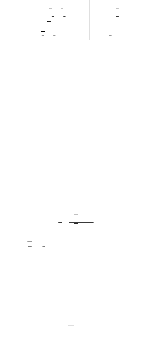
Method Strongly convex Non-strongly convex
GD O
L
µ
log
1
ε
[33] O
L
ε
[33]
heavy-ball O
q
L
µ
log
1
ε
[35] O
L
ε
[37]
AGD O
q
L
µ
log
1
ε
[8], [33] O
q
L
ε
[8], [33], [38], [51]
Lower Bounds O
q
L
µ
log
1
ε
[33], [66], [67] O
q
L
ε
[33], [66], [67]
TABLE I
ITERATION COMPLEXITY COMPARISONS BETWEEN GD, THE HEAVY-BALL
METHOD AND AGD, AS WELL AS THE LOWER BOUNDS.
E. Lower Bound
Can we find algorithms faster than AGD? Better yet, how
fast can we solve problem (1), or its simplified case
min
x∈R
p
f(x), (7)
to some accuracy
ε
, using methods only based on the infor-
mation of
∇f(x)
? A few existing bounds can answer these
questions. The first lower bounds for first-order optimization
algorithms were given in [65], and then were extended in [33].
We introduce the widely used conclusion in [33]. Consider any
iterative first-order method generating a sequence of points
{x
t
}
k
t=0
such that
x
k
∈ x
0
+ Span{∇f(x
0
), ··· , ∇f (x
k−1
)}. (8)
[33] constructed a special
L
-smooth and
µ
-strongly convex
function
f(x)
such that for any sequence satisfying (8), we
have
f(x
k
) − f(x
∗
) ≥
µ
2
√
L −
√
µ
√
L +
√
µ
!
2k
kx
0
− x
∗
k
2
.
It means that any first-order method satisfying (8) needs at
least
O
q
L
µ
log
1
ε
iterations to achieve an
ε
-optimal solution
for the class of
L
-smooth and
µ
-strongly convex problems.
Recalling the upper bound given in Section
II-C
, we can see
that it matches this lower bound. Thus, Nesterov’s AGDs are
optimal and they cannot be further accelerated up to constants.
When the strong-convexity is absent, [33] constructed another
L
-smooth convex function
f(x)
such that for any method
satisfying (8), we have
f(x
k
) − f(x
∗
) ≥
3L
32(k + 1)
2
kx
0
− x
∗
k
2
,
kx
k
− x
∗
k
2
≥
1
32
kx
0
− x
∗
k
2
.
The iteration number
k
for the counterexample in [33]
depends on the dimension
p
of the problem, e.g.,
k
should
satisfy
k ≤
1
2
(p − 1)
for non-strongly convex problems. [66],
[68] proposed a different framework to establish the same
lower bounds as [33], but, the iteration number in [66], [68]
is dimension-independent. When considering the composite
problem (1), we can use the results in [67] to give the same
lower bounds as [33] for first-order methods that are only
based on the information of
∇f(x)
and
Prox
h
(z)
. Although
[67] studied the finite-sum problem, their conclusion can be
used to (1) as long as
f(x) 6= 0
,
h(x) 6= 0
, and
f(x) 6= h(x)
.
For better comparison of different methods, we list the
iteration complexities as well as the lower bounds in Table I.
III. ACCELERATED STOCHASTIC ALGORITHMS
In machine learning, people often encounter big data with
extremely large
n
in problem (1). Computing the full gradient of
f(x)
in GD and AGD might be expensive. Stochastic gradient
algorithms might be the most common way to cope with big
data. They sample, in each iteration, one or several gradients
from individual functions as an estimator of the full gradient
of f. For example, consider the standard proximal Stochastic
Gradient Descent (SGD), which uses one stochastic gradient
at each iteration and proceeds as follows
x
k+1
= Prox
η
k
h
x
k
− η
k
∇f
i
k
(x
k
)
,
where
η
k
denotes the step-size and
i
k
is an index randomly
sampled from
{1, . . . , n}
at iteration
k
. SGD often suffers
from slow convergence. For example, when the objective is
L
-smooth and
µ
-strongly convex, SGD only obtains a sublinear
rate [69] of
E[F (x
k
)] − F (x
∗
) ≤ O (1/k) .
In contrast, GD has the linear convergence. In the following
sections, we introduce several techniques to accelerate SGD.
Especially, we discuss how Nesterov’s acceleration works in
stochastic optimization with finite
n
in problem (1), which is
often called the finite-sum problem.
A. Variance Reduction and Its Acceleration
The main challenge for SGD is the noise of the randomly-
drawn gradients. The variance of the noisy gradient will never
go to zero even if
x
k
→ x
∗
. As a result, one has to gradually cut
down the step-size in SGD to guarantee convergence, which
brings down the convergence. A technique called Variance
Reduction (VR) [70] was designed to reduce the negative
effect of noise. For finite-sum objective functions, the VR
technique reduces the variance to zero through the updates. The
first VR method might be Stochastic Average Gradient (SAG)
[71], which uses the sum of the latest individual gradients
as an estimator of the descent direction. It requires
O(np)
memory storage and uses a biased gradient estimator. Stochastic
Variance Reduced Gradient (SVRG) [70] reduces the memory
cost to
O(p)
and uses an unbiased gradient estimator. Later,
SAGA [72] improves SAG by using an unbiased update via
the technique of SVRG. Other VR methods can be found in
[73]–[78].
We take SVRG [79] as an example, which is relatively simple
and easy to implement. SVRG maintains a snapshot vector
˜
x
s
after every
m
SGD iterations and keeps the gradient of the
averages
g
s
= ∇f(
˜
x
s
)
. Then, it uses
˜
∇f(x
k
) = ∇f
i
k
(x
k
) −
∇f
i
k
(
˜
x
s
)+ g
s
as the descent direction at every SGD iterations,
and the expectation
E
i
k
[
˜
∇f(x
k
)] = ∇f(x
k
)
. Moreover, the
variance of the estimated gradient
˜
∇f(x
s,k
)
now can be upper
bounded by the distance from the snapshot vector to the latest
variable, i.e.,
E[k
˜
∇f(x
k
)−∇f (x
k
)k
2
] ≤ Lkx
k
−
˜
x
s
k
2
, which
is a crucial property of SVRG to guarantee the reduction of
variance. Algorithm 1 gives the details of SVRG.

JOURNAL OF L
A
T
E
X CLASS FILES, VOL. 14, NO. 8, AUGUST 2015 5
Algorithm 1 SVRG
Input
˜
x
0
, m = O(L/µ), and η = O(1/L).
for s = 0, 1, 2, ··· do
x
0
=
˜
x
s
,
g
s
= ∇f(
˜
x
s
),
for k = 0, ··· , m do
Randomly sample i
k
from {1, . . . , n},
˜
∇f(x
k
) = ∇f
i
k
(x
k
) − ∇f
i
k
(
˜
x
s
) + g
s
,
x
k+1
= Prox
ηh
x
k
− η
˜
∇f(x
k
)
,
end for
˜
x
s+1
=
1
m
P
m
k=1
x
k
,
end for
For
µ
-strongly convex problem (1) with
L
-smooth
f
i
(x)
,
SVRG needs
O
L
µ
log
1
ε
inner iterations to reach an
ε
-optimal
solution in expectation. Each inner iteration needs to evaluate
two stochastic gradients while each outer iteration needs
additional
n
individual gradient evaluations to compute
g
s
.
Thus, the gradient complexity of SVRG is
O
n +
L
µ
log
1
ε
.
Recall that GD has the gradient complexity of
O
nL
µ
log
1
ε
,
since it needs
n
individual gradient evaluations at each iteration.
Thus, SVRG is superior to GD when L/µ > 1.
With the VR technique in hand, one can fuse it with Nes-
terov’s acceleration technique to further accelerate stochastic
algorithms, e.g., [10]–[13], [80], [81]. We take Katyusha [10]
as an example. Katyusha builds upon the combination of (6a)-
(6c) and SVRG. Different from (6a) and (6c), Katyusha further
introduces a “negative momentum” with additional
τ
0
˜
x
s
in
(10a) and (10d), which prevents the extrapolation term from
being far from the snapshot vector. Algorithm 2 gives the
details of Katyusha.
Algorithm 2 Katyusha
Input
x
0
= z
0
=
˜
x
0
,
m = n
,
τ = min{
p
nµ
3L
,
1
2
}
,
τ
0
=
1
2
,
η = O(
1
L
), and τ
00
=
µ
3τL
+ 1.
for s = 0, 1, 2, ··· do
g
s
= ∇f(
˜
x
s
)
for k = 0, ··· , m do
y
k
= τz
k
+ τ
0
˜
x
s
+ (1 − τ − τ
0
)x
k
, (10a)
Randomly sample i
k
from {1, . . . , n},
˜
∇f(y
k
) = ∇f
i
k
(y
k
) − ∇f
i
k
(
˜
x
s
) + g
s
, (10b)
z
k+1
= Prox
ηh/τ
z
k
− η/τ
˜
∇f(y
k
)
, (10c)
x
k+1
= τz
k+1
+ τ
0
˜
x
s
+ (1 − τ − τ
0
)x
k
, (10d)
end for
˜
x
s+1
=
P
m−1
k=0
(τ
00
)
k
−1
P
m−1
k=0
(τ
00
)
k
x
k
,
z
0
= x
m
, x
0
= x
m
,
end for
For problems with smooth and convex
f
i
(x)
and
µ
-
strongly convex
h(x)
, the gradient complexity of Katyusha is
O
n +
q
nL
µ
log
1
ε
. When
n ≤ O(L/µ)
, Katyusha further
accelerates SVRG. Comparing SVRG with Katyusha, we can
see that the only difference is that Katyusha uses the mechanism
of AGD in (6a)-(6c). Thus, Nesterov’s acceleration technique
also takes effect in finite-sum stochastic optimization.
We now describe several extensions of Katyusha with some
advanced topics.
1) Loopless Katyusha: Both SVRG and Katyusha have
double loops, which make them a little complex to analyze
and implement. To remedy the double loops, [12] proposed a
loopless SVRG and Katyusha for the simplified problem
min
x∈R
p
f(x)
def
=
1
n
n
X
i=1
f
i
(x) (11)
with smooth and convex
f
i
(x)
, and strongly convex
f(x)
.
Specifically, at each iteration, with a small probability
1/n
, the
methods update the snapshot vector and perform a full pass over
data to compute the average gradient. With probability
1−1/n
,
the methods use the previous snapshot vector. The loopless
SVRG and Katyusha enjoy the same gradient complexities
as the original methods. We take the loopless SVRG as an
example, which consists of the following steps at each iteration,
˜
∇f(x
k
) = ∇f
i
k
(x
k
) − ∇f
i
k
(
˜
x
k
) + ∇f(
˜
x
k
), (12a)
x
k+1
= x
k
− η
˜
∇f(x
k
), (12b)
˜
x
k+1
=
x
k
with probability 1/n,
˜
x
k
with probability 1 −1/n.
(12c)
When replacing (12a) and (12b) by the following steps, we
get the loopless Katyusha,
y
k
= τz
k
+ τ
0
˜
x
k
+ (1 − τ − τ
0
)x
k
,
˜
∇f(y
k
) = ∇f
i
k
(y
k
) − ∇f
i
k
(
˜
x
k
) + ∇f(
˜
x
k
),
z
k+1
=
1
αµ/L + 1
αµ
L
y
k
+ z
k
−
α
L
˜
∇f(y
k
)
,
x
k+1
= τz
k+1
+ τ
0
˜
x
s
+ (1 − τ − τ
0
)x
k
,
where we set
τ = min
q
2nµ
3L
, 1/2
,
τ
0
= 1/2
, and
α =
2
3τ
.
2) Non-Strongly Convex Problems: When the strong con-
vexity assumption is absent, the gradient complexities of
SGD and SVRG are
O
1
ε
2
[82] and
O
n log
1
ε
+
L
ε
[83],
respectively. Katyusha improves the complexity of SVRG
to
O
n
q
F (x
0
)−F (x
∗
)
ε
+
q
nLkx
0
−x
∗
k
2
ε
[10], [11]. This
gradient complexity is not more advantageous over Nesterov’s
full batch AGD since they all need
O
n
√
ε
individual gradient
evalutions. When applying reductions to extend the algorithms
designed for smooth and strongly convex problems to non-
strong convex ones, e.g., the HOOD framework [84], the
gradient complexity of Katyusha can be further improved to
O
n log
1
ε
+
q
nL
ε
, which is
√
n
times faster than the full
batch AGD when high precision is required. On the other hand,
[13] proposed a unified VR accelerated gradient method, which
employs a direct acceleration scheme instead of employing
any reduction to obtain the desired gradient complexity of
O
n log n +
q
nL
ε
.
JOURNAL OF L
A
T
E
X CLASS FILES, VOL. 14, NO. 8, AUGUST 2015 6
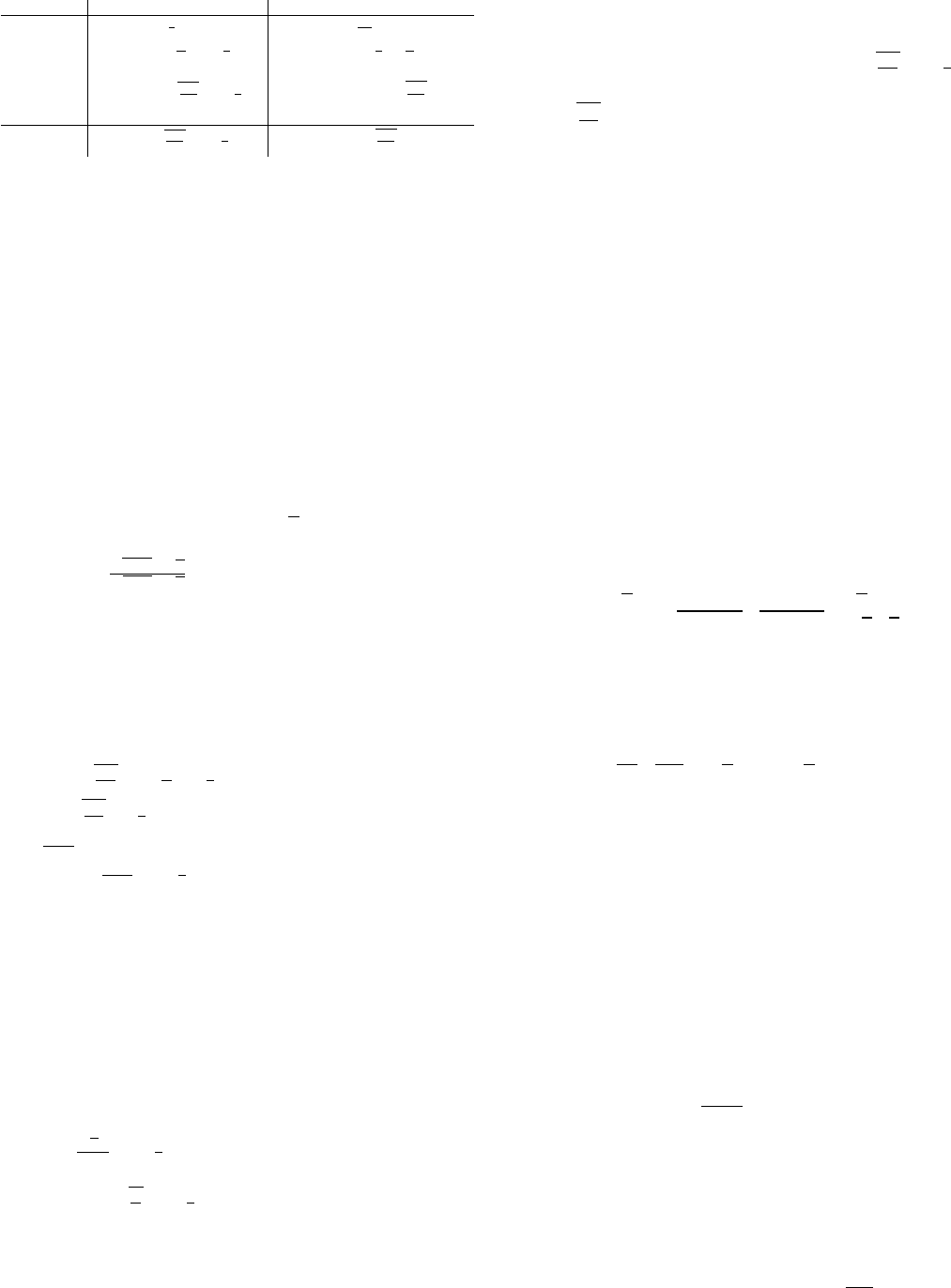
Method Smooth and Strongly Convex Smooth and Non-strongly Convex
SGD O
1
ε
[69] O
1
ε
2
[82]
SVRG O
n +
L
µ
log
1
ε
O
n log
1
ε
+
L
ε
[12], [70]–[72] [83]
AccVR O
n +
q
nL
µ
log
1
ε
O
n log n +
q
nL
ε
[10]–[13] [13]
Lower bounds O
n +
q
nL
µ
log
1
ε
[67] O
n +
q
nL
ε
[67]
TABLE II
GRADIENT COMPLEXITY COMPARISONS BETWEEN SGD, SVRG AND
ACCELERATED VR METHODS (ACCVR), AS WELL AS THE LOWER BOUNDS.
3) Universal Catalyst Acceleration for First-Order Convex
Optimization: Another way to accelerate SVRG is to use
the universal Catalyst [85], which is a unified framework to
accelerate first-order methods. It builds upon the accelerated
proximal point method with inexactly computed proximal
mapping. Analogous to (5a)-(5b), Catalyst takes the following
outer iterations
y
k
= x
k
+ β
k
(x
k
− x
k−1
), (14a)
x
k
≈ argmin
x∈R
p
n
G
k
(x)
def
= F (x) +
γ
2
kx − y
k
k
2
o
, (14b)
where
β
k
=
√
γ+µ−
√
µ
√
γ+µ+
√
µ
for strongly convex problems, and
it updates in the same way as that in (5a)-(5b) for non-
strongly convex ones. We can use any linearly-convergent
method that is only based on the information of
∇f
i
(x)
and
Prox
h
(z)
to approximately solve the subproblem in (14b).
The subproblem often has a good condition number and so
can be solved efficiently to a high precision. Take SVRG as
an example. When we use SVRG to solve the subproblem,
Catalyst accelerates SVRG to the gradient complexity of
O
n +
q
nL
µ
log
L
µ
log
1
ε
for strongly convex problems
and
O
q
nL
ε
log
1
ε
for non-strongly convex ones, by setting
γ =
L−µ
n+1
− µ
and the inner iteration number in step (14b)
as
O
n +
L+γ
µ+γ
log
1
ε
with
µ ≥ 0
and
L ≥ (n + 2)µ
.
Besides SVRG, Catalyst can also accelerate other methods, e.g.,
SAG and SAGA. The price for generality is that the gradient
complexities of Catalyst have an additional poly-logarithmic
factor compared with those of Katyusha.
4) Individually Nonconvex: Some problems in machine
learning can be written as minimizing strongly convex functions
that are finite average of nonconvex ones [75], [77]. That is,
each
f
i
(x)
in problem (11) is
L
-smooth and may be nonconvex,
but their average
f(x)
is
µ
-strongly convex. Examples include
the core machinery for PCA and SVD. SVRG can also be
used to solve this problem with the gradient complexity of
O
n +
√
nL
µ
log
1
ε
[80]. [80] further proposed a method
named KatyushaX to improve the gradient complexity to
O
n + n
3/4
q
L
µ
log
1
ε
.
5) Lower Complexity Bounds: Similar to the lower bounds
for the class of deterministic first-order algorithms, there are
also lower bounds for the randomized first-order methods for
finite-sum problems. Considering problem (11), [67] proved
that for any first-order algorithm that is only based on the infor-
mation of
∇f
i
(x)
and
Prox
f
i
(z)
, the lower bound for
L
-smooth
and
µ
-strongly convex problems is
O
n +
q
nL
µ
log
1
ε
.
When the strong convexity is absent, the lower bound becomes
O
n +
q
nL
ε
. For better comparison, we list the upper and
lower bounds in Table II.
6) Application to Distributed Optimization: Variance reduc-
tion has also been applied to distributed optimization. Classical
distributed algorithms include the distributed gradient descent
(DGD) [86], EXTRA [87], the gradient-tracking-based methods
[88]–[91], and distributed stochastic gradient descent (DSGD)
[92], [93]. To further improve the convergence of stochastic
distributed algorithms, [94] combined EXTRA with SAGA,
[95] combined gradient tracking with SAGA, and [95], [96]
implemented gradient tracking in SVRG. See [97] for a detailed
review. It is an interesting work to implement accelerated VR
in distributed optimization in the future.
B. Stochastic Coordinate Descent and Its Acceleration
In problem (1), we often assume that
f
i
(x)
is smooth and
allow
h(x)
to be nondifferentiable. However, not all machine
learning problems satisfy this assumption. The typical example
is SVM, which can be formulated as
min
x∈R
p
F (x)
def
=
1
n
n
X
i=1
max
0, 1 − y
i
A
T
i
x
| {z }
f
i
(x)
+
µ
2
kxk
2
| {z }
h(x)
. (15)
We can see that each
f
i
(x)
is convex but nondifferentiable,
and
h(x)
is smooth and strongly convex. In practice, we often
minimize the negative of the dual of (15), written as
min
u∈R
n
D(u)
def
=
1
2µ
e
Au
n
2
−
1
n
n
X
i=1
u
i
+
1
n
n
X
i=1
I
[0,1]
(u
i
), (16)
where
e
A
i
= y
i
A
i
, and
I
[0,1]
(u) = 0
if
0 ≤ u ≤ 1
, and
∞
, otherwise. Motivated by (16), we consider the following
problem in this section
min
u∈R
n
D(u)
def
= Φ(u) +
n
X
i=1
Ψ
i
(u
i
). (17)
We assume that
Φ(u)
satisfies the coordinate-wise smooth
condition
k∇
i
Φ(u) − ∇
i
Φ(v)k ≤ L
i
ku − vk
for any
u
and
v
satisfying
u
j
= v
j
, ∀j 6= i
. We also assume that
Φ(u)
is
µ
-strongly convex with respect to norm
k · k
L
, i.e., replacing
ky−xk
2
in (2) by
ky−xk
2
L
=
P
n
i=1
L
i
(y
i
−x
i
)
2
. We require
Ψ
i
(u)
to be convex but can be nondifferentiable. Take problem
(16) as an example,
L
i
=
k
e
A
i
k
2
n
2
µ
, but the first term in (16) is
not strongly convex when n > p.
Stochastic Coordinate Descent (SCD) is a popular method to
solve problem (17). It first computes the partial derivative with
respect to one randomly chosen variable, and then updates this
variable by a coordinate-wise gradient descent while keeping
the other variables unchanged. SCD is sketched as follows:
u
k+1
i
k
= argmin
u
Ψ
i
k
(u) +
∇
i
k
Φ(u
k
), u
+
L
i
k
2
|u −u
k
i
k
|
2
,

JOURNAL OF L
A
T
E
X CLASS FILES, VOL. 14, NO. 8, AUGUST 2015 7
where
i
k
is randomly sampled form
{1, . . . , n}
. In SCD, we
often assume that the proximal mapping of
Ψ
i
(u)
can be
efficiently computed with a closed solution. Also, we need to
compute
∇
i
k
Φ(u
k
)
efficiently. Take problem (16) for example,
by keeping track of
s
k
=
e
Au
k
and updating
s
k+1
by
s
k
−
e
A
i
k
u
k
i
k
+
e
A
i
k
u
k+1
i
k
, SCD only uses one column of
e
A
per
iteration, i.e., one sample, to compute
∇
i
k
Φ(u
k
) =
1
n
2
µ
e
A
T
i
k
s
k
.
Now, we come to the convergence rate of SCD [98], which
is described as
E[D(u
k
)] − D(u
∗
) ≤ min
1 −
µ
n
k
,
n
n + k
C (18)
in a unified style for strongly convex and non-strongly convex
problems, where C = D(u
0
) − D(u
∗
) + ku
0
− u
∗
k
2
L
.
We can also perform Nesterov’s acceleration technique to
accelerate SCD by combing it with (6a)-(6c). When
Φ(u)
in
(17) is strongly convex, the resultant method is called Acceler-
ated randomized Proximal Coordinate Gradient (APCG) [16],
and it is described in Algorithm 3. When the strong convexity
assumption is absent, the method is called Accelerated Parallel
PROXimal coordinate descent (APPROX) [15], and it is written
in Algorithm 4, where
θ
k
> 0
is obtained by solving equation
θ
2
k
= (1 −θ
k
)θ
2
k−1
, which is initialized as
θ
0
= 1/n
. Specially,
APPROX reduces to (6a)-(6c) when
n = 1
. Both APCG and
APPROX have a faster convergence rate than SCD, which is
given as follows in a unified style
E[D(u
k
)] − D(u
∗
) ≤ min
(
1 −
√
µ
n
k
,
2n
2n + k
2
)
C,
where C is given in (18).
Algorithm 3 APCG
Input u
0
= z
0
.
for k = 0, 1, ··· do
y
k
=
1
1 +
√
µ/n
u
k
+
√
µ
n
z
k
, (19a)
Randomly sample i
k
from {1, . . . , n}
z
k+1
i
k
= argmin
z
Ψ
i
k
(z) +
∇
i
k
Φ(y
k
), z
(19b)
+
L
i
k
√
µ
2
z −
1 −
√
µ
n
z
k
i
k
−
√
µ
n
y
k
i
k
2
!
,
z
k+1
j
= z
k
j
, ∀j 6= i
k
, (19c)
u
k+1
= y
k
+
√
µ
z
k+1
− z
k
+
µ
n
z
k
− y
k
, (19d)
end for
1) Efficient Implementation: Both APCG and APPROX need
to perform full-dimensional vector operations in steps (19a),
(19d), (20a), and (20d), which make the per-iteration cost
higher than that of SCD, where the latter one only needs
to consider one dimension per iteration. This may cause the
overall computational cost of APCG and APPROX higher than
that of the full AGD. To avoid such an situation, we can use a
change of variables scheme, which is firstly proposed in [99]
and then adopted by [15], [16]. Take APPROX as an example.
We only need to introduce an auxiliary variable
ˆ
u
k
initialized
Algorithm 4 APPROX
Input u
0
= z
0
.
for k = 0, 1, ··· do
y
k
= (1 − θ
k
)u
k
+ θ
k
z
k
, (20a)
Randomly sample i
k
from {1, . . . , n}
z
k+1
i
k
= argmin
z
Ψ
i
k
(z) +
∇
i
k
Φ(y
k
), z
(20b)
+
nθ
k
L
i
k
2
kz − z
k
i
k
k
2
,
z
k+1
j
= z
k
j
, ∀j 6= i
k
, (20c)
u
k+1
= y
k
+ nθ
k
z
k+1
− z
k
, (20d)
end for
at
0
and change the updates by the following ones at each
iteration
z
k+1
i
k
= argmin
z
Ψ
i
k
(z) +
∇
i
k
Φ(z
k
+ θ
2
k
ˆ
u
k
), z
+
nθ
k
L
i
k
2
kz − z
k
i
k
k
2
,
ˆ
u
k+1
i
k
=
ˆ
u
k
i
k
−
1 − nθ
k
θ
2
k
(z
k+1
i
k
− z
k
i
k
),
ˆ
u
k+1
j
=
ˆ
u
k
j
, z
k+1
j
= z
k
j
, ∀j 6= i
k
.
The partial gradient
∇
i
k
Φ(z
k
+ θ
2
k
ˆ
u
k
)
can be efficiently
computed in a similar way to that of SCD discussed above
with almost no more burden.
2) Applications to the Regularized Empirical Risk Mini-
mization: Now, we consider the regularized empirical risk
minimization problem, which is a special case of problem (1)
and is described as
min
x∈R
p
F (x)
def
=
1
n
n
X
i=1
g
i
(A
T
i
x) + h(x). (22)
We often normalize the columns of
A
to have unit norm.
Motivated by (16), we minimize the negative of the dual of
(22) as
min
u∈R
n
D(u)
def
= h
∗
Au
n
+
1
n
n
X
i=1
g
∗
i
(−u
i
), (23)
where
h
∗
(u) = max
v
{hu, vi−h(v)}
is the convex conjugate
of
h
. For some applications in machine learning, e.g., SVM,
∇
i
h
∗
(Au/n)
and
Prox
g
∗
i
(u)
can be efficiently computed [100]
and we can use APCG and APPROX to solve (23). When
g
i
is
L
-smooth and
h
is
µ
-strongly convex, APCG needs
O
n +
q
nL
µ
log
1
ε
iterations to obtain an
ε
-approximate
expected dual gap
E[F (x
k
)] + E[D(u
k
)] ≤ ε
[16]. When the
smoothness assumption on g
i
is absent, the required iteration
number of APPROX is
O
n log n +
p
n
for the expected
ε
dual gap [18].
One limitation of the SCD-based methods is that they require
computing
∇
i
h
∗
(Au/n)
and
Prox
g
∗
i
(u)
, rather than
Prox
h
(x)
and
∇g
i
(A
T
i
x)
. In some applications, e.g., regularized logistic
regression, the SCD-based methods need inner loops and they
are less efficient than the VR-based methods. However, for

JOURNAL OF L
A
T
E
X CLASS FILES, VOL. 14, NO. 8, AUGUST 2015 8
other applications where the VR-based methods cannot be used,
e.g.,
g
i
is nonsmooth, the SCD-based method may be a better
choice, especially when
h
is chosen as the
`
2
regularizer and
the proximal mapping of g
i
is simple.
3) Restart for SVM under the Quadratic Growth Condition:
In machine learning, some problems may satisfy a condition
that is weaker than strong convexity and stronger than convexity,
namely the quadratic growth condition [101]. For example,
the dual problem of SVM [102]. Can we expect a faster
convergence than the sublinear rate of
O(1/k)
or
O(1/k
2
)
?
The answer is yes. Some studies have shown that the accelerated
methods with restart [103]–[105] enjoy a linear convergence
under the quadratic growth condition. Generally speaking, if
we have an accelerated method with an
O
1
k
2
rate at hand,
e.g., APPROX, we can run the method without any change
and restart it after several iterations with warm-starts. If we set
the restart period according to the quadratic growth condition
constant, a similar constant to the condition number in the
strong convexity assumption, the resultant method converges
with a linear rate, which is faster than the non-accelerated
counterparts. Moreover, when the quadratic growth condition
constant is unknown (it is often the case in practice), [18],
[104], [105] showed that the method also converges linearly,
but the rate may not be optimal.
4) Non-uniform Sampling: In problem (16), we have
L
i
=
k
e
A
i
k
2
n
2
µ
. For the analysis in Section
III-B
2, we normalize the
columns of
e
A
to have unit norm and
L
i
have the same values
for all
i
. When they are not normalized, a variety of works have
focused on the non-uniform sampling of the training sample
i
k
[99], [106]–[108]. For example, [107] selected the
i
-th
sample with probability proportional to
√
L
i
and obtained better
performance than the uniform sampling scheme. Intuitively
speaking, when
L
i
is large, the function is less smooth along
the
i
-th coordinate, so we should sample it more often to
balance the overall convergence speed.
C. The Primal-Dual Method and Its Accelerated Stochastic
Variants
The VR-based methods and SCD-based methods perform
in the primal space and the dual space, respectively. In this
section, we introduce another common scheme, namely, the
primal-dual-based methods [46], [47], which perform both in
the primal space and the dual space. Consider problem (22).
It can be written in the min-max form:
min
x∈R
p
max
u∈R
n
1
n
n
X
i=1
A
T
i
x, u
i
− g
∗
i
(u
i
)
+ h(x). (24)
We first introduce the general primal-dual method with Breg-
man distance to solve problem (24) [20], which consists of the
following steps at each iteration
ˆ
x
k
=α(x
k
− x
k−1
) + x
k
, (25a)
u
k+1
=argmax
u
1
n
A
T
ˆ
x
k
,u
−
1
n
n
X
i=1
g
∗
i
(u
i
)−τD(u, u
k
)
!
,
(25b)
x
k+1
=argmin
x
h(x)+
x,
1
n
Au
k+1
+
η
2
kx−x
k
k
2
, (25c)
for constants
α
,
τ
, and
η
to be specified later and
x
−1
= x
0
.
The primal-dual method alternately maximizes
u
in the dual
space and minimizes x in the primal space.
As explained in Section III, dealing with all the samples
at each iteration is time-consuming when
n
is large, so we
want to handle only one sample. Accordingly, we can sample
only one
i
k
randomly in (25b) at each iteration. The resultant
method is described in Algorithm 5, and it reduces to the
Stochastic Primal Dual Coordinate (SPDC) method proposed
in [19] when we take
D(u, v) =
1
2
(u − v)
2
as a special case.
Combining the initialization
s
0
=
1
n
Au
0
and the update rules
(26c) and (26e), we know s
k
=
1
n
Au
k
.
Algorithm 5 SPDC
Input
x
0
= x
−1
,
τ =
2
√
nµL
,
η = 2
√
nµL
, and
α = 1 −
1
n+2
√
nL/µ
for k = 0, 1, ··· do
ˆ
x
k
= α(x
k
− x
k−1
) + x
k
, (26a)
u
k+1
i
k
= argmax
u
A
T
i
k
ˆ
x
k
, u
− g
∗
i
k
(u) − τD(u − u
k
i
k
)
,
(26b)
u
k+1
j
= u
k
j
, ∀j 6= i
k
, (26c)
x
k+1
= argmin
x
h(x)+
x, s
k
+(u
k+1
i
k
−u
k
i
k
)A
i
k
+
η
2
kx − x
k
k
2
, (26d)
s
k+1
= s
k
+
1
n
(u
k+1
i
k
− u
k
i
k
)A
i
k
, (26e)
end for
Similar to APCG, when each
g
i
is
L
-smooth,
h
is
µ
-strongly
convex, and the columns of
A
are normalized to have unit
norm, SPDC needs
O
n +
q
nL
µ
log
1
ε
iterations to find
a solution such that E[kx
k
− x
∗
k
2
] ≤ ε.
One limitation of SPDC is that it only applies to problems
when the proximal mappings of
g
∗
i
and
h
can be efficiently
computed. In some applications, we want to use
∇g
i
, rather
than
Prox
g
∗
i
. To remedy this problem, [20] creatively used
the Bregman distance induced by
g
∗
i
in (26b). Specifically,
taking
ϕ
in (3) as
g
∗
i
k
, letting
z
k−1
i
k
=
ˆ
∇g
∗
i
k
(u
k
i
k
)
and defining
z =
A
T
i
k
ˆ
x
k
+τz
k−1
i
k
1+τ
, step (26b) reduces to
u
k+1
i
k
= argmax
u
D
A
T
i
k
ˆ
x
k
+ τ
ˆ
∇g
∗
i
k
(u
k
i
k
), u
E
−(1 + τ )g
∗
i
k
(u)
= argmax
u
hz, ui − g
∗
i
k
(u)
= ∇g
i
k
(z).
Then, we have
z ∈ ∂g
∗
i
k
(u
k+1
i
k
)
and denote it as
z
k
i
k
. Thus, we
can replace steps (26b) and (26c) by the following two steps
z
k
j
=
(
A
T
j
ˆ
x
k
+τz
k−1
j
1+τ
, j = i
k
,
z
k−1
j
, j 6= i
k
,
u
k+1
j
=
∇g
j
(z
k
j
), j = i
k
,
u
k
j
, j 6= i
k
.
Accordingly, the resultant method, named the Randomized
Primal-Dual Gradient (RPDG) method [20], is only based
on
∇g
j
(z)
and the proximal mapping of
h(x)
. To find an

JOURNAL OF L
A
T
E
X CLASS FILES, VOL. 14, NO. 8, AUGUST 2015 9
ε
-optimal solution, it needs the same number of iterations as
SPDC but each iteration has the same computational cost as
the VR-based methods, e.g., Katyusha.
1) Relation to Nesterov’s AGD: It is interesting to study
the relation between the primal-dual method and Nesterov’s
accelerated gradient method. [20] proved that (25a)-(25c) with
τ
k
= (1 − θ
k
)/θ
k
,
η
k
= Lθ
k
,
α
k
= θ
k
/θ
k−1
, and appropriate
Bregman distance reduces to (6a)-(6c) when solving (22), where
we use adaptive parameters in (25a)-(25c). Thus, RPDG can
also be seen as an extension of Nsterov’s AGD to finite-sum
stochastic optimization problems.
2) Non-strongly Convex Problems: When the strong con-
vexity assumption on
h(x)
is absent, [76] studied the
O
1
√
ε
iteration upper bound for the stochastic primal-dual hybrid
gradient algorithm, which is a variant of SPDC. However, no
explicit dependence on
n
was given in [76]. On the other
hand, the perturbation approach is a popular way to obtain
sharp convergence results for non-strongly convex problems.
Specifically, define a perturbation problem by adding a small
perturbation term
εkx
0
− xk
2
to problem (22), and solve it
by RPDG, which is developed for strongly convex problems.
However, the resultant gradient complexity has an additional
term
log
1
ε
as compared with the lower bound in [67] and
the upper bound in [13]. Since the conditions in the HOOD
framework [84] may not be satisfied for RPDG due to the dual
term, currently the reduction approach introduced in Section
III-A
2 has not been applied to the primal-dual-based methods
to remove the additional poly-logarithmic factor.
IV. ACCELERATED NONCONVEX ALGORITHMS
In this section, we introduce the generalization of accel-
eration to nonconvex problems. Specifically, Section
IV-A
introduces the deterministic algorithms and Section
IV-B
for
the stochastic ones.
A. Deterministic Algorithms
In the following two sections, we describe the algorithms to
find first-order and second-order stationary points, respectively.
1) Achieving First-Order Stationary Point: Gradient descent
and its proximal variant are widely used in machine learning,
both for convex and noncovnex applications. For nonconvex
problems, GD finds an
ε
-approximate first-order stationary
point within O
1
ε
2
iterations [33].
Motivated by the success of heavy-ball method, [109] studied
its nonconvex extension with the name of iPiano. Specifically,
consider problem (1) with smooth (possibly nonconvex)
f(x)
and convex
h(x)
(possibly nonsmooth), and the heavy-ball
method (4) with
β ∈ [0, 1)
and
η <
2(1−β)
L
. [109] proved
that any limit point
x
∗
of
x
k
is a critical point of (1), i.e.,
0 ∈ ∇f(x
∗
) + ∂h(x
∗
)
. Moreover, the number of iterations to
find an ε-approximate first-order stationary point is O
1
ε
2
.
Besides the heavy-ball method, some researchers studied
the nonconvex accelerated gradient method extended from
Nesterov’s AGD. For example, [110] studied the following
method for problem (1) with convex h(x):
y
k
= (1 − θ
k
)x
k
+ θ
k
z
k
, (27a)
z
k+1
= Prox
δ
k
h
z
k
− δ
k
∇f(y
k
)
, (27b)
x
k+1
= Prox
σ
k
h
y
k
− σ
k
∇f(y
k
)
, (27c)
which is motivated by (6a)-(6c). In fact, when
h(x) = 0
,
δ
k
=
1
Lθ
k
, and
σ
k
=
1
L
, (6a)-(6c) and (27a)-(27c) are equivalent.
[110] proved that (27a)-(27c) needs
O
1
ε
2
iterations to find an
ε
-approximate first-order stationary point by setting
θ
k
=
2
k+1
,
σ
k
=
1
2L
, and
σ
k
≤ δ
k
≤ (1 + θ
k
/4)σ
k
. On the other hand,
when
f(x)
is also convex, (27a)-(27c) has the optimal
O
1
√
ε
iteration complexity to find an
ε
-optimal solution by a different
setting of δ
k
=
kσ
k
2
.
Although (27a)-(27c) guarantees the convergence for non-
convex programming while maintaining the acceleration for
convex programming, one disadvantage is that the parameter
settings for convex and noncovnex problems are different. To
address this issue, [111] proposed the following method:
y
k
= x
k
+
θ
k
θ
k−1
(z
k
− x
k
) +
θ
k
(1 − θ
k−1
)
θ
k−1
(x
k
− x
k−1
),
z
k+1
= Prox
ηh
(y
k
− η∇f(y
k
)),
v
k+1
= Prox
ηh
(x
k
− η∇f(x
k
)),
x
k+1
=
z
k+1
, if F (z
k+1
) ≤ F (v
k+1
),
v
k+1
, otherwise,
which is motivated by the monotone AGD proposed in [112].
Intuitively, the first two steps perform a proximal AGD update
with the same update rule of
θ
k
as that in (5a)-(5b), the
third step performs a proximal GD update, and the last step
chooses the one with the smaller objective. Similar to the
heavy ball method, [112] proved that any limit point of
x
k
a critical point, and the method needs
O
1
ε
2
iterations
to find an
ε
-approximate first-order stationary point. On
the other hand, when both
f(x)
and
h(x)
are convex, the
same
O
1
√
ε
iteration complexity as Nesterov’s AGD is
maintained. Moreover, the algorithm for convex programming
and nonconvex programming keeps the same parameters. The
price paid is that the computational cost per iteration of the
above method is higher than that of (27a)-(27c).
Besides the above algorithms, Nesterov has also extended his
AGD to nonconvex programming [42]. Similar to the geometric
descent [48] discussed in Section
II-D
, Nesterov’s method also
needs a line search and thus it is not a rigorously “first-order”
method.
We can see that none of the above algorithms have provable
improvement after adopting the technique of heavy-ball method
or Nesterov’s AGD. One may ask: can we find a provable faster
accelerated gradient method for nonconvex programming?
The answer is yes. [22] proposed a method which achieves
an
ε
-approximate first-order stationary point within
O
1
ε
7/4
gradient and function evaluations. The algorithm in [22] is
complex to implement, so we omit the details.
2) Achieving Second-Order Stationary Point: We first dis-
cuss whether gradient descent can find the approximate second-
order stationary point. To answer this question, [113] studied
a simple variant of GD with appropriate perturbations and
JOURNAL OF L
A
T
E
X CLASS FILES, VOL. 14, NO. 8, AUGUST 2015 10
showed that the method achieves an
O(ε, O(
√
ε))
-approximate
second-order stationary point within
e
O(1/ε
2
)
iterations, where
e
O
hides the poly-logarithmic factors. We can see that this rate
is exactly the rate of GD to first-order stationary point, with
only the additional log factor. The method proposed in [113]
is given in Algorithm 6, where
Uniform(B
0
(r))
means the
perturbation uniformly sampled from a ball with radius r.
Algorithm 6 Perturbed GD
Input
x
0
= z
,
p = 0
,
T =
e
O(
1
√
ε
)
,
r =
e
O(ε)
,
η = O(
1
L
)
, and
ε
0
= O(ε
1.5
).
for k = 0, 1, ··· do
if k∇f(x
k
)k ≤ ε
and
k > p + T
(i.e., no perturbation in
last T steps) then
z = x
k
, p = k
x
k
= x
k
+ ξ
k
, ξ
k
∼ Uniform(B
0
(r)),
end if
x
k+1
= x
k
− η∇f(x
k
),
if k = p + T and f (z) − f (x
k
) ≤ ε
0
then
break,
end if
end for
Intuitively speaking, when the norm of the current gradient
is small, it indicates that the current iterate is potentially near
a saddle point or a local minimum. If it is near a saddle point,
the uniformly distributed perturbation helps to escape it, which
is added at most once in every
T
iterations. On the other hand,
when the objective almost does not decrease after
T
iterations
from last perturbation, it achieves the local minimum with high
probability and we can stop the algorithm.
Besides [113], [114] showed that the plain GD without per-
turbations almost always escapes saddle points asymptotically.
However, it may take exponential time [115].
Now, we come to the accelerated gradient method. Built upon
Algorithm 6 and (5a)-(5b), [24] proposed a variant of AGD
with perturbations and showed that the method needs
O
1
ε
7/4
iterations to achieve an
(ε, O(
√
ε))
-approximate second-order
stationary point, which is faster than the perturbed GD. We
describe the method in Algorithm 7, where the NCE (Negative
Curvature Exploitation) step chooses
x
k+1
to be
x
k
+ δ
or
x
k
− δ
whichever having a smaller objective
f
, where
δ =
sv
k
/kv
k
k for some constant s.
In the above scheme, the first “if” step is similar to the
perturbation step in the perturbed GD. The following three
steps are similar to the AGD steps in (5a)-(5b), where
v
k
is the
momentum term in (5a). When the function has large negative
curvature between
x
k
and
y
k
, i.e., the second “if” condition
holds, NCE simply moves along the direction based on the
momentum.
Besides [24], [21] and [23] also established the
O
1
ε
7/4
gradient complexity to achieve an
ε
-approximate second-order
stationary point. [21] employed a combination of (regularized)
AGD and the Lanczos method, and [23] proposed a careful im-
plementation of the Nesterov-Polyak method, using accelerated
methods for fast approximate matrix inversion.
At last, we compare the iteration complexity of the ac-
Algorithm 7 Perturbed AGD
Input
x
0
,
v
0
,
T =
e
O(
1
ε
1/4
)
,
r =
e
O(ε)
,
β =
e
O(1 − ε
1/4
)
,
η = O(
1
L
), γ =
e
O(
√
ε) and s =
e
O(
√
ε).
for k = 0, 1, ··· do
if k∇f(x
k
)k≤ε
and no perturbation in last
T
steps,
then
x
k
= x
k
+ ξ
k
, ξ
k
∼ Uniform(B
0
(r)),
end if
y
k
= x
k
+ βv
k
,
x
k+1
= y
k
− η∇f(y
k
),
v
k+1
= x
k+1
− x
k
,
if f(x
k
)≤f(y
k
)+
∇f(y
k
), x
k
−y
k
−
γ
2
kx
k
−y
k
k
2
then
(x
k+1
, v
k+1
) = NCE(x
k
, v
k
),
end if
end for
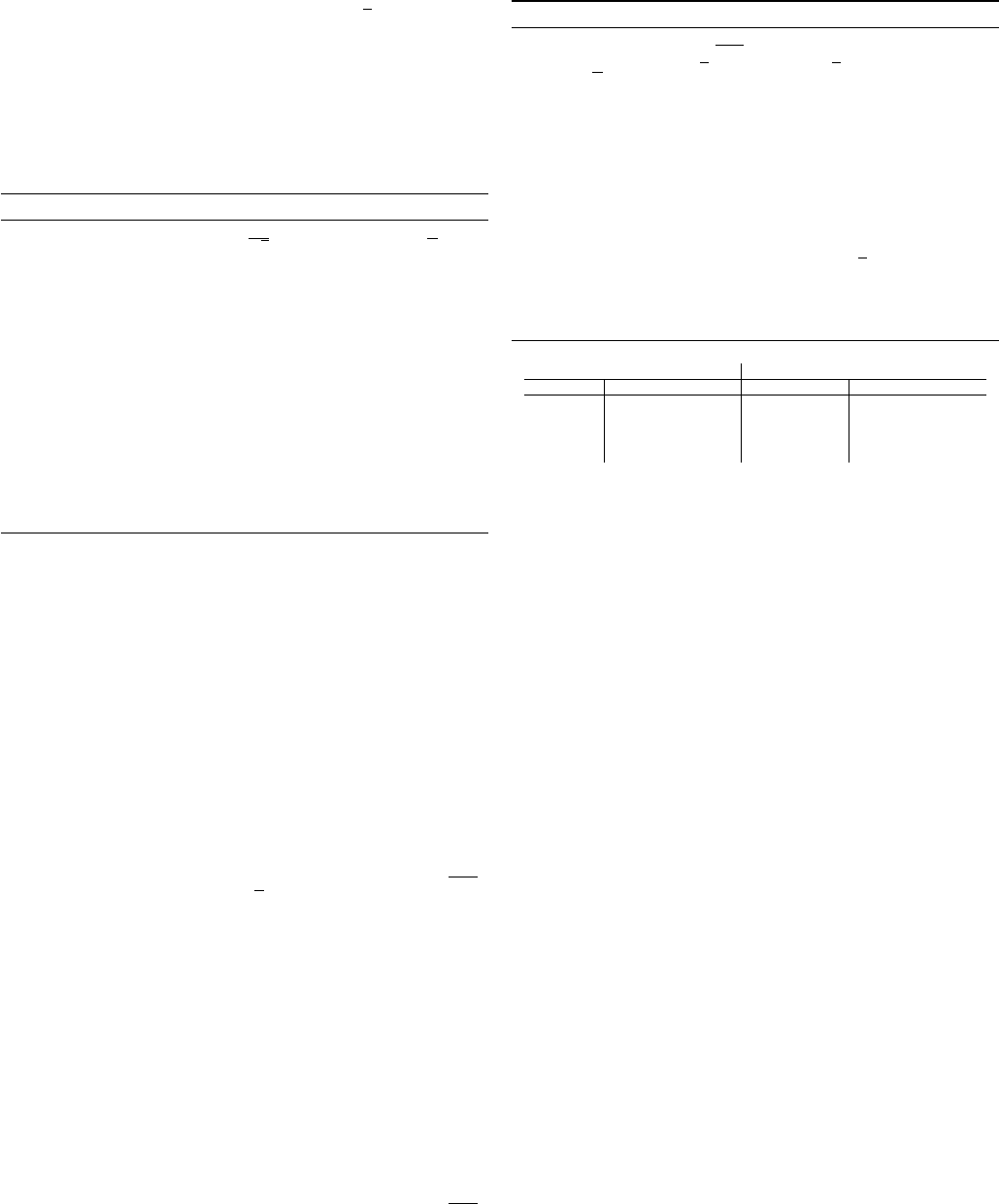
First-order Stationary Point Second-order Stationary Point
Methods Iteration Complexity Methods Iteration Complexity
GD [33] O(1/ε
2
) Perturbed GD
e
O(1/ε
2
)
[113]
AGD [22]
e
O(1/ε
7/4
) AGD
e
O(1/ε
7/4
)
[21], [23], [24]
TABLE III
ITERATION COMPLEXITY COMPARISONS BETWEEN GRADIENT DESCENT
AND ACCELERATED GRADIENT DESCENT FOR NONCONVEX PROBLEMS. WE
HIDE THE POLY-LOGARITHMIC FACTORS IN
e
O
. WE ALSO HIDE
n
SINCE WE
ONLY CONSIDER DETERMINISTIC OPTIMIZATION.
celerated methods and non-accelerated methods in Table III,
including both the approximation of first-order stationary point
and second-order stationary point.
B. Stochastic Algorithms
Due to the success of deep neural network, in recent years
people are interested in stochastic algorithms for nonconvex
problem (1) or (11) with huge
n
, especially the accelerated
variants. [116] empirically observed that the following plain
stochastic AGD performs well when training deep neural
networks:
y
k
= x
k
+ β
k
(x
k
− x
k−1
),
x
k+1
= y
k
− η∇f
i
k
(y
k
),
where β
k
is empirically set as
β
k
= min{1 − 2
−1−log
2
(bk/250c+1)
, β
max
},
and β
max
is often chosen as 0.999 or 0.995.
In this section, we introduce the stochastic nonconvex
algorithms with more theory supports than the above plain
stochastic AGD. For simplicity, we consider problem (11) with
each f
i
(x) being L-smooth.
1) Achieving First-Order Stationary Point: When we assume
that the variance of the gradient is finite, SGD requires the
gradient complexity of
O(ε
−4
)
to achieve an
ε
-approximate
first-order stationary point [33]. Similar to stochastic convex
optimization, this bound can be further improved by VR.
In fact, a sight variant of the SVRG algorithm [117]–[119]
and also SAGA [120] achieve the gradient complexity of
O
n + n
2/3
ε
−2
∧ ε
−10/3
, where
a ∧ b = min(a, b)
. This

JOURNAL OF L
A
T
E
X CLASS FILES, VOL. 14, NO. 8, AUGUST 2015 11
result means that when
n → ∞
, the VR technique can
still guarantee a faster convergence rate in the nonconvex
stochastic optimization, where we refer this case as the online
optimization. However, this bound is still not optimal and
it can be further reduced to
O
n + n
1/2
ε
−2
∧ ε
−3
by
performing recursive VR [26], [78], [121]–[123]. We take
the Stochastic Path-Integrated Differential Estimator (SPIDER)
[26] algorithm as an example. SPIDER can be used for both the
finite-sum problem (11) and the online problem. For simplicity,
we consider the following simplified method for the finite-sum
problem, as shown in Algorithm 8.
Algorithm 8 SPIDER
for k = 0 to K do
v
k
=
∇f(x
k
), if mod(k, n)=0,
∇f
i
k
(x
k
)−∇f
i
k
(x
k−1
)+v
k−1
, otherwise.
η
k
= min
ε
L
√
nkv
k
k
,
1
2L
√
n
,
x
k+1
= x
k
− η
k
v
k
.
end for
SPIDER is motivated by SVRG, but using a different VR
technique. We can compare SPIDER with the loopless SVRG
(12a)-(12c) to be more intuitive. SPIDER takes steps along
the direction based on past accumulated stochastic gradient
information, i.e.,
v
k
=
k
X
t=k
0
+1
∇f
i
t
(x
t
) − ∇f
i
t
(x
t−1
)
+ v
k
0
for the latest
k
0
such that
mod (k
0
, n) = 0
and
v
k
0
= ∇f(x
k
0
)
.
In contrast, SVRG takes steps only based on the information
of current stochastic gradient and the snapshot vector, i.e.,
v
k
= ∇f
i
k
(x
k
) − ∇f
i
k
(
˜
x
s
) + ∇f(
˜
x
s
)
. It was shown in [26]
that the variance of
v
k
is smaller than that in the SVRG
algorithm by order when
x
k
moves slowly, which contributes
to a provably faster convergence rate.
The recursive VR technique was firstly proposed in the
algorithm named SARAH in [78], which was designed for
convex optimization and then was extended to nonconvex
optimization [123]. For the finite-sum smooth optimization,
SPIDER and SARAH almost have the same algorithm form.
They are different in the step-size. SARAH uses
η = O(
1
L
√
n
)
while SPIDER uses a normalized but more conservative step-
size (at the order of
O(ε)
). After [26], some improved versions,
such as SpiderBoost [122], also considered allowing a larger
step-size.
As for the lower bounds, [26] proved that the gradient
complexity of
O(n+ n
1/2
ε
−2
)
matches the lower bound under
certain conditions. More recently, [124] showed that
O(ε
−3
)
also matches the lower bound when n → ∞.
2) Achieving Second-order Stationary Point: When the
objective function is assumed to have a Lipschitz continuous
Hessian matrix, acceleration has also been done to find an
approximate second-order stationary point. For example, [23],
[27] converted the cubic regularization method [131] for finding
a second-order stationary point using stochastic-gradient-based
and Hessian-vector-product-based methods. [129], [130] pro-
posed a generic saddle-point-escaping method called NEON,
which approximates Hessian-vector product by stochastic
gradient. For the convergence rate, to search an
(ε, O(ε
0.5
))
-
approximate second-order stationary point, in the finite-sum
case, the VR and the momentum techniques [21], [23] can
reduce the gradient complexity to
e
O(nε
−1.5
+ n
3/4
ε
−1.75
)
. In
the online case, [125] first proved that noisy SGD escapes
from saddle points in polynomial times. Later, [126] obtained
a gradient complexity of
e
O(ε
−10
)
. This bound was finally
improved by [128], in which the authors proved that noisy
SGD can actually find a second-order stationary point within
the gradient complexity of
e
O(ε
−3.5
)
. For the variants of SGD,
by fusing negative curvature search with VR, for finding an
(ε, O(ε
0.25
))
-approximate second-order stationary point, [25]
obtained a lower gradient complexity of
e
O(ε
−3.25
)
. When
using the SPIDER [26] technique, one can obtain a complexity
of
e
O(ε
−3
)
to find an
(ε, O(ε
0.5
))
-approximate second-order
stationary point. Table IV summarizes the gradient complexity
comparisons of the existing algorithms.
V. DISCUSSION AND LIMITATION
Accelerated algorithms have been widely used in machine
learning due to their provably faster convergence and simplicity
in implementation. In this paper, we review the accelerated
deterministic algorithms, accelerated stochastic algorithms
and accelerated nonconvex algorithms for machine learning.
Due to space limit, our review is incomplete as we have
left some interesting topics out, e.g., the acceleration for
distributed optimization [132]–[142]. Its challenge over the
non-distributed algorithms introduced in this paper is that we
should pay attention to the agreement among different nodes.
Modifications are required to extend the classical AGD to
distributed optimization.
The efficiency of accelerated algorithms have been verified
in practice for convex optimization, either deterministic or
stochastic. However, in reality some complex accelerated
nonconvex algorithms seem less efficient. One remarkable
example is that although they are proven to converge faster to
first-order or second-order stationary points than SGD, when
training deep neural networks, they still cannot beat SGD or
the plain stochastic AGD. There is still a gap between theory
and practice for accelerated nonconvex optimization.
REFERENCES
[1]
C. Cortes and V. Vapnik, “Support-vector networks,” Machine Learning,
vol. 20, pp. 273–297, 1995.
[2]
J. Berkson, “Application of the logistic function to bio-assay,” Journal
of the American Statistical Association, vol. 39, no. 227, pp. 357–365,
1944.
[3]
R. Tibshirani, “Regression shrinkage and selection via the lasso,” Journal
of the Royal Statistical Society. Series B (Methodological), vol. 58, no. 1,
pp. 267–288, 1996.
[4]
S. Haykin, Neural Networks: A Comprehensive Foundation. Prentice
Hall, Englewood Cliffs, NJ, 2 ed., 1999.
[5]
Y. Nesterov, “A method for unconstrained convex minimization problem
with the rate of convergence
O(1/k
2
)
,” Doklady AN SSSR, vol. 269,
pp. 543–547, 1983.
[6]
Y. Nesterov, “On an approach to the construction of optimal methods of
minimization of smooth convex functions,”
`
Ekonomika I Mateaticheskie
Metody, vol. 24, pp. 509–517, 1988.

JOURNAL OF L
A
T
E
X CLASS FILES, VOL. 14, NO. 8, AUGUST 2015 12
Type Algorithm Online Finite-Sum
First-order
Stationary Point
Original SGD / GD [33] O(ε
−4
) O(nε
−2
)
Acceleration
SVRG / SCSG /SAGA [117]–[120] O
ε
−10/3
O
n + n
2/3
ε
−2
SPIDER / SpiderBoost / SARAH [26], [121]–[123] O
ε
−3
O
n + n
1/2
ε
−2
Second-order
Stationary Point
(Hessian-smooth
Required)
Original Perturbed GD / SGD
[125]
[126]
[113], [127]
[128]
e
O
poly(d)ε
−4
e
O
ε
−10
e
O
ε
−4
e
O
ε
−3.5
not given
not given
e
O
nε
−2
not given
Acceleration
NEON+GD/SGD [129], [130]
e
O(ε
−4
)
e
O(nε
−2
)
Perturbed AGD [24] not given nε
−1.75
NEON+VR [25], [117]–[119]
e
O
ε
−3.5
e
O
nε
−1.5
+ n
2/3
ε
−2
NEON+VR+Momentum [21], [23], [27]
e
O
ε
−3.5
e
O
nε
−1.5
+ n
3/4
ε
−1.75
NEON+SPIDER [26]
e
O
ε
−3
e
O
n + n
1/2
−2
TABLE IV
GRADIENT COMPLEXITY COMPARISONS BETWEEN DIFFERENT ACCELERATED STOCHASTIC ALGORITHMS AND THEIR NON-ACCELERATED COUNTERPARTS
TO FIND AN
ε
-APPROXIMATE FIRST-ORDER STATIONARY POINT OR AN
(ε, O(ε
0.5
))
-APPROXIMATE SECOND-ORDER STATIONARY POINT FOR NONCONVEX
PROBLEMS.
[7]
Y. Nesterov, “Smooth minimization of non-smooth functions,” Mathe-
matical Programming, vol. 103, pp. 127–152, 2005.
[8]
Y. Nesterov, “Gradient methods for minimizing composite functions,”
Mathematical Programming, vol. 140, pp. 125–161, 2013.
[9]
Z. Lin, H. Li, and C. Fang, Accelerated Optimization in Machine
Learning: First-Order Algorithms. Springer, 2020.
[10]
Z. Allen-Zhu, “Katyusha: The first direct acceleration of stochastic
gradient methods,” Journal of Machine Learning Research, vol. 18,
no. 221, pp. 1–51, 2018.
[11]
K. Zhou, F. Shang, and J. Cheng, “A simple stochastic variance reduced
algorithm with fast convergence rates,” in International Conference on
Machine Learning (ICML), pp. 5975–5984, 2019.
[12] D. Kovalev, S. Horv
´
ath, and P. Richt
´
arik, “Don’t jump through hoops
and remove those loops: SVRG and Katyusha are better without the
outer loop,” in International Conference on Algorithmic Learning Theory
(ALT), pp. 451–467, 2020.
[13]
G. Lan, Z. Li, and Y. Zhou, “A unified variance-reduced accelerated
gradient method for convex optimization,” in Advances in Neural
Information Processing Systems (NeurIPS), pp. 10462–10472, 2019.
[14]
Y. Nesterov, “Efficiency of coordinate descent methods on huge-scale
optimization problems,” SIAM Journal on Optimization, vol. 22, no. 2,
pp. 341–362, 2012.
[15]
O. Fercoq and P. Richt
´
arik, “Accelerated, parallel, and proximal
coordinate descent,” SIAM Journal on Optimization, vol. 25, no. 4,
pp. 1997–2023, 2015.
[16]
Q. Lin, Z. Lu, and L. Xiao, “An accelerated randomized proximal
coordinate gradient method and its application to regularized empirical
risk minimization,” SIAM Journal on Optimization, vol. 25, no. 4,
pp. 2244–2273, 2015.
[17]
S. Shalev-Shwartz and T. Zhang, “Accelerated proximal stochastic dual
coordinate ascent for regularized loss minimization,” Mathematical
Programming, vol. 155, pp. 105–145, 2016.
[18]
H. Li and Z. Lin, “On the complexity analysis of the primal solutions
for the accelerated randomized dual coordinate ascent,” Journal of
Machine Learning Research, vol. 21, no. 33, pp. 1–45, 2020.
[19]
Y. Zhang and L. Xiao, “Stochastic primal-dual coordinate method for
regularized empirical risk minimization,” Journal of Machine Learning
Research, vol. 18, no. 84, pp. 1–42, 2017.
[20]
G. Lan and Y. Zhou, “An optimal randomized incremental gradient
method,” Mathematical Programming, vol. 171, pp. 167–215, 2018.
[21]
Y. Carmon, J. C. Duchi, O. Hinder, and A. Sidford, “Accelerated
methods for nonconvex optimization,” SIAM Journal on Optimization,
vol. 28, no. 2, pp. 1751–1772, 2018.
[22]
Y. Carmon, J. C. Duchi, O. Hinder, and A. Sidford, “Convex until
proven guilty: Dimension-free acceleration of gradient descent on non-
convex functions,” in International Conference on Machine Learning
(ICML), pp. 654–663, 2017.
[23]
N. Agarwal, Z. Allen-Zhu, B. Bullins, E. Hazan, and T. Ma, “Finding
approximate local minima faster than gradient descent,” in ACM
Symposium on Theory of Computing (STOC), pp. 1195–1199, 2017.
[24]
C. Jin, P. Netrapalli, and M. I. Jordan, “Accelerated gradient descent
escapes saddle points faster than gradient descent,” in Conference On
Learning Theory (COLT), pp. 1042–1085, 2018.
[25]
Z. Allen-Zhu, “Natasha2: Faster non-convex optimization than SGD,”
in Advances in Neural Information Processing Systems (NeurIPS),
pp. 2675–2686, 2018.
[26]
C. Fang, C. J. Li, Z. Lin, and T. Zhang, “SPIDER: Near-optimal non-
convex optimization via stochastic path integrated differential estimator,”
in Advances in Neural Information Processing Systems (NeurIPS),
pp. 689–699, 2018.
[27]
N. Tripuraneni, M. Stern, C. Jin, J. Regier, and M. I. Jordan, “Stochastic
cubic regularization for fast nonconvex optimization,” in Advances in
Neural Information Processing Systems (NeurIPS), pp. 2899–2908,
2018.
[28]
S. Bhojanapalli, B. Neyshabur, and N. Srebro, “Global optimality of
local search for low rank matrix recovery,” in Advances in Neural
Information Processing Systems (NIPS), pp. 3873–3881, 2016.
[29]
R. Ge, J. D. Lee, and T. Ma, “Matrix completion has no spurious local
minimum,” in Advances in Neural Information Processing Systems
(NIPS), pp. 2973–2981, 2016.
[30]
R. Ge, C. Jin, and Y. Zheng, “No spurious local minima in nonconvex
low rank problems: A unified geometric analysis,” in International
Conference on Machine Learning (ICML), pp. 1233–1242, 2017.
[31]
A. Choromanska, M. Henaff, M. Mathieu, G. B. Arous, and Y. LeCun,
“The loss surfaces of multilayer networks,” in International Conference
on Machine Learning (ICML), pp. 192–204, 2015.
[32]
K. Kawaguchi, “Deep learning without poor local minima,” in Advances
in Neural Information Processing Systems (NIPS), pp. 586–594, 2016.
[33]
Y. Nesterov, Introductory Lectures on Convex Optimization: A Basic
Course. Kluwer Academic, Boston, 2004.
[34]
B. T. Polyak, “Some methods of speeding up the convergence of iteration
methods,” USSR Computational Mathematics and Mathematical Physics,
vol. 4, no. 5, pp. 1–17, 1964.
[35]
P. Ochs, T. Brox, and T. Pock, “iPiasco: Inertial proximal algorithm
for strongly convex optimization,” Journal of Mathematical Imaging
and Vision, vol. 53, pp. 171–181, 2015.
[36]
L. Lessard, B. Recht, and A. Packard, “Analysis and design of
optimization algorithms via integral quadratic constraints,” SIAM Journal
on Optimization, vol. 26, no. 1, pp. 57–95, 2016.
[37]
E. Ghadimi, H. R. Feyzmahdavian, and M. Johansson, “Global
convergence of the heavy-ball method for convex optimization,” in
European Control Conference (ECC), pp. 310–315, 2015.
[38]
A. Beck and M. Teboulle, “A fast iterative shrinkage-thresholding
algorithm for linear inverse problems,” SIAM Journal on Imaging
Sciences, vol. 2, no. 1, pp. 183–202, 2009.
[39]
W. Su, S. Boyd, and E. Cand
`
es, “A differential equation for modeling
Nesterov’s accelerated gradient method: Theory and insights,” Journal
of Machine learning Research, vol. 17, no. 153, pp. 1–43, 2016.
[40]
S. Safavi, B. Joshi, G. Franca, and J. Bento, “An explicit convergence
rate for Nesterov’s method from SDP,” in Innovations in Theoretical
Computer Science (ITCS), 2018.
[41]
A. Wibisono, A. C. Wilson, and M. I. Jordan, “A variational perspective
on accelerated methods in optimization,” Proceedings of the National
Academy of Sciences, vol. 113, no. 47, pp. 7351–7358, 2016.
[42]
Y. Nesterov, A. Gasnikov, S. Guminov, and P. Dvurechensky, “Primal-
JOURNAL OF L
A
T
E
X CLASS FILES, VOL. 14, NO. 8, AUGUST 2015 13
dual accelerated gradient methods with small-dimensional relaxation
oracle,” arXiv:1809.05895, 2018.
[43]
P. Tseng, “On accelerated proximal gradient methods for convex-concave
optimization,” tech. rep., University of Washington, Seattle, 2008.
[44]
C. Fang, Y. Huang, and Z. Lin, “Accelerating asynchronous algo-
rithms for convex optimization by momentum compensation,” arX-
iv:1802.09747, 2018.
[45]
Z. Allen-Zhu and L. Orecchia, “Linear coupling: An ultimate unification
of gradient and mirror descent,” in Innovations in Theoretical Computer
Science (ITCS), 2017.
[46]
A. Chambolle and T. Pock, “A first-order primal-dual algorithm for
convex problems with applications to imaging,” Journal of Mathematical
Imaging and Vision, vol. 40, pp. 120–145, 2011.
[47]
A. Chambolle and T. Pock, “On the ergodic convergence rates of a
first-order primal-dual algorithm,” Mathematical Programming, vol. 159,
pp. 253–287, 2016.
[48]
S. Bubeck, Y. T. Lee, and M. Singh, “A geometric alternative to
Nesterov’s accelerated gradient descent,” arXiv:1506.08187, 2015.
[49]
D. Drusvyatskiy, M. Fazel, and S. Roy, “An optimal first order method
based on optimal quadratic averaging,” SIAM Journal on Optimization,
vol. 28, no. 1, pp. 251–271, 2018.
[50]
Y. Drori and M. Teboulle, “Performance of first-order methods for
smooth convex minimization: a novel approach,” Mathematical Pro-
gramming, vol. 145, pp. 451–482, 2014.
[51]
D. Kim and J. A. Fessler, “Optimized first-order methods for smooth
convex minimization,” Mathematical Programming, vol. 159, pp. 81–
107, 2016.
[52]
G. Lan, “Gradient sliding for composite optimization,” Mathematical
Programming, vol. 159, pp. 201–235, 2016.
[53]
G. Lan and Y. Zhou, “Conditional gradient sliding for convex optimiza-
tion,” SIAM Journal on Optimization, vol. 26, no. 2, pp. 1379–1409,
2016.
[54]
G. Lan and Y. Ouyang, “Accelerated gradient sliding for structured
convex optimization,” preprint arXiv:1609.04905, 2016.
[55]
G. Lan and R. D. Monteiro, “Iteration-complexity of first-order
penalty methods for convex programming,” Mathematical Programming,
vol. 138, pp. 115–139, 2013.
[56]
Y. Chen, G. Lan, and Y. Ouyang, “Optimal primal-dual methods for a
class of saddle point problems,” SIAM Journal on Optimization, vol. 24,
no. 4, pp. 1779–1814, 2014.
[57]
Y. Xu, “Accelerated first-order primal-dual proximal methods for
linearly constrained composite convex programming,” SIAM Journal
on Optimization, vol. 27, no. 3, pp. 1459–1484, 2017.
[58]
Y. Ouyang, Y. Chen, G. Lan, and E. Pasiliao Jr, “An accelerated
linearized alternating direction method of multipliers,” SIAM Journal
on Imaging Sciences, vol. 8, no. 1, pp. 644–681, 2015.
[59]
H. Li and Z. Lin, “Accelerated alternating direction method of
multipliers: an optimal
O(1/K)
nonergodic analysis,” Journal of
Scientific Computing, vol. 79, pp. 671–699, 2019.
[60]
J. Lu and M. Johansson, “Convergence analysis of approximate primal
solutions in dual first-order methods,” SIAM Journal on Optimization,
vol. 26, no. 4, pp. 2430–2467, 2016.
[61]
B. He and X. Yuan, “On the acceleration of augmented Lagrangian
method for linearly constrained optimization,” Optimization Online,
2010.
[62]
T. Goldstein, B. O’Donoghue, S. Setzer, and R. Baraniuk, “Fast
alternating direction optimization methods,” SIAM Journal on Imaging
Sciences, vol. 7, no. 3, pp. 1588–1623, 2014.
[63]
P. Giselsson and S. Boyd, “Linear convergence and metric selection
for Douglas-Rachford splitting and ADMM,” IEEE Transactions on
Automatic Control, vol. 62, no. 2, pp. 532–544, 2016.
[64]
G. Franca and J. Bento, “An explicit rate bound for over-relaxed
ADMM,” in IEEE International Symposium on Information Theory
(ISIT), pp. 2104–2108, 2016.
[65]
A. Nemriovsky and D. Yudin, Problem complexity and method efficiency
in optimization. Willey-Interscience, New York, 1983.
[66]
Y. Arjevani and O. Shamir, “On the iteration complexity of oblivious
first-order optimization algorithms,” in International Conference on
Machine Learning (ICML), pp. 654–663, 2016.
[67]
B. Woodworth and N. Srebro, “Tight complexity bounds for optimizing
composite objectives,” in Advances in Neural Information Processing
Systems (NIPS), pp. 3639–3647, 2016.
[68]
Y. Arjevani, S. Shalev-Shwartz, and O. Shamir, “On lower and upper
bounds for smooth and strongly convex optimization,” Journal of
Machine Learning Research, vol. 17, no. 126, pp. 1–51, 2016.
[69]
L. Bottou, F. E. Curtis, and J. Nocedal, “Optimization methods for
large-scale machine learning,” SIAM Review, vol. 60, no. 2, pp. 223–311,
2018.
[70]
R. Johnson and T. Zhang, “Accelerating stochastic gradient descent
using predictive variance reduction,” in Advances in Neural Information
Processing Systems (NIPS), pp. 315–323, 2013.
[71]
M. Schmidt, N. Le Roux, and F. Bach, “Minimizing finite sums with
the stochastic average gradient,” Mathematical Programming, vol. 162,
pp. 83–112, 2017.
[72]
A. Defazio, F. Bach, and S. Lacoste-Julien, “SAGA: A fast incremental
gradient method with support for non-strongly convex composite
objectives,” in Advances in Neural Information Processing Systems
(NIPS), pp. 1646–1654, 2014.
[73]
L. Zhang, M. Mahdavi, and R. Jin, “Linear convergence with condition
number independent access of full gradients,” in Advances in Neural
Information Processing Systems (NIPS), pp. 980–988, 2013.
[74]
A. Defazio, T. Caetano, and J. Domke, “Finito: A faster, permutable
incremental gradient method for big data problems,” in International
Conference on Machine Learning (ICML), pp. 1125–1133, 2014.
[75]
J. Mairal, “Optimization with first-order surrogate functions,” in
International Conference on Machine Learning (ICML), pp. 783–791,
2013.
[76]
A. Chambolle, M. J. Ehrhardt, P. Richt
´
arik, and C.-B. Sch
¨
onlieb,
“Stochastic primal-dual hybrid gradient algorithm with arbitrary sampling
and imaging applications,” SIAM Journal on Optimization, vol. 28, no. 4,
pp. 2783–2808, 2018.
[77]
S. Shalev-Shwartz, “SDCA without duality, regularization, and indi-
vidual convexity,” in International Conference on Machine Learning
(ICML), pp. 747–754, 2016.
[78]
L. M. Nguyen, J. Liu, K. Scheinberg, and M. Tak
´
ac, “SARAH: A
novel method for machine learning problems using stochastic recursive
gradient,” in International Conference on Machine Learning (ICML),
pp. 2613–2621, 2017.
[79]
L. Xiao and T. Zhang, “A proximal stochastic gradient method with
progressive variance reduction,” SIAM Journal on Optimization, vol. 24,
no. 4, pp. 2057–2075, 2014.
[80]
Z. Allen-Zhu, “Katyusha X: Practical momentum method for stochas-
tic sum-of-nonconvex optimization,” in International Conference on
Machine Learning (ICML), pp. 179–185, 2019.
[81]
A. Defazio, “A simple practical accelerated method for finite sums,” in
Advances in Neural Information Processing Systems (NIPS), pp. 676–
684, 2016.
[82]
O. Shamir and T. Zhang, “Stochastic gradient descent for non-smooth
optimization: Convergence results and optimal averaging schemes,” in
International Conference on Machine Learning (ICML), pp. 71–79,
2013.
[83]
Z. Allen-Zhu and Y. Yuan, “Improved SVRG for non-strongly-convex or
sum-of-non-convex objectives,” in International Conference on Machine
Learning (ICML), pp. 1080–1089, 2016.
[84]
Z. Allen-Zhu and E. Hazan, “Optimal black-box reductions between
optimization objectives,” in Advances in Neural Information Processing
Systems (NIPS), pp. 1614–1622, 2016.
[85]
H. Lin, J. Mairal, and Z. Harchaoui, “Catalyst acceleration for first-
order convex optimization: from theory to practice,” Journal of Machine
Learning Research, vol. 18, no. 212, pp. 1–54, 2018.
[86]
A. Nedi
´
c and A. Ozdaglar, “Distributed subgradient methods for multi-
agent optimization,” IEEE Transactions on Automatic Control, vol. 54,
no. 1, pp. 48–61, 2009.
[87]
W. Shi, Q. Ling, G. Wu, and W. Yin, “EXTRA: An exact first-order
algorithm for decentralized consensus optimization,” SIAM Journal on
Optimization, vol. 25, no. 2, pp. 944–966, 2015.
[88]
J. Xu, S. Zhu, Y. C. Soh, and L. Xie, “Augmented distributed gradient
methods for multi-agent optimization under uncoordinated constant
stepsizes,” in IEEE Conference on Decision and Control (CDC),
pp. 2055–2060, 2015.
[89]
G. Qu and N. Li, “Harnessing smoothness to accelerate distributed
optimization,” IEEE Transactions on Control of Network Systems, vol. 5,
no. 3, pp. 1245–1260, 2018.
[90]
A. Nedi
´
c, A. Olshevsky, and W. Shi, “Achieving geometric convergence
for distributed optimization over time-varying graphs,” SIAM Journal
on Optimization, vol. 27, no. 4, pp. 2597–2633, 2017.
[91]
R. Xin, U. A. Khan, and S. Kar, “A linear algorithm for optimization over
directed graphs with geometric convergence,” IEEE Control Systems
Letters, vol. 2, no. 3, pp. 315–320, 2018.
[92]
J. Chen and A. H. Sayed, “Diffusion adaptation strategies for distributed
optimization and learning over networks,” IEEE Transactions on Signal
Processing, vol. 60, no. 8, pp. 4289–4305, 2012.
JOURNAL OF L
A
T
E
X CLASS FILES, VOL. 14, NO. 8, AUGUST 2015 14
[93]
S. S. Ram, A. Nedi
´
c, and V. V. Veeravalli, “Distributed stochastic
subgradient projection algorithms for convex optimization,” Journal of
Optimization Theory and Applications, vol. 147, pp. 516–545, 2010.
[94]
A. Mokhtari and A. Ribeiro, “DSA: Decenrtalized double stochastic
averaging gradient algorithm,” Journal of Machine Learning Research,
vol. 17, no. 61, pp. 1–35, 2016.
[95]
R. Xin, U. A. Khan, and S. Kar, “Variance-reduced decentralized
stochastic optimization with accelerated convergence,” preprint arX-
iv:1912.04230, 2019.
[96]
B. Li, S. Cen, Y. Chen, and Y. Chi, “Communication-efficient dis-
tributed optimization in networks with gradient tracking,” preprint
arXiv:1909.05844 (to appear in Journal of Machine Learning Research),
2020.
[97]
R. Xin, S. Kar, and U. A. Khan, “Decentralized stochastic optimization
and machine learning: A unified variance-reduction framework for
robust performance and fast convergence,” IEEE Signal Processing
Magazine, vol. 37, no. 3, pp. 102–113, 2020.
[98]
Z. Lu and L. Xiao, “On the complexity analysis of randomized block-
coordinate descent methods,” Mathematical Programming, vol. 152,
pp. 615–642, 2015.
[99]
Y. T. Lee and A. Sidford, “Efficient accelerated coordinate descent
methods and faster algorithms for solving linear systems,” in IEEE
Symposium on Foundations of Computer Science (FOCS), pp. 147–156,
2013.
[100]
S. Shalev-Shwartz and T. Zhang, “Stochastic dual coordinate ascent
methods for regularized loss minimization,” Journal of Machine
Learning Research, vol. 14, pp. 567–599, 2013.
[101]
I. Necoara, Y. Nesterov, and F. Glineur, “Linear convergence of first
order methods for non-strongly convex optimization,” Mathematical
Programming, vol. 175, pp. 69–107, 2019.
[102]
P. W. Wang and C. J. Lin, “Iteration complexity of feasible descent
methods for convex optimization,” Journal of Machine Learning
Research, vol. 15, pp. 1523–1548, 2014.
[103]
B. O’Donoghue and E. Cand
`
es, “Adaptive restart for accelerated gradient
schemes,” Foundations of Computational Mathematics, vol. 15, pp. 715–
732, 2015.
[104]
O. Fercoq and Z. Qu, “Adaptive restart of accelerated gradient methods
under local quadratic growth condition,” IMA Journal of Numerical
Analysis, vol. 39, no. 4, pp. 2069–2095, 2019.
[105]
O. Fercoq and Z. Qu, “Restarting the accelerated coordinate descent
method with a rough strong convexity estimate,” Computational
Optimization and Applications, vol. 75, pp. 63–91, 2020.
[106]
Z. Qu, P. Richt
´
arik, and T. Zhang, “Quartz: Randomized dual coordinate
ascent with arbitrary sampling,” in Advances in Neural Information
Processing Systems (NIPS), pp. 865–873, 2015.
[107]
Z. Allen-Zhu, Z. Qu, P. Richt
´
arik, and Y. Yuan, “Even faster accelerated
coordinate descent using non-uniform sampling,” in International
Conference on Machine Learning (ICML), pp. 1110–1119, 2016.
[108]
Y. Nesterov and S. U. Stich, “Efficiency of the accelerated coordinate
descent method on structured optimization problems,” SIAM Journal
on Optimization, vol. 27, no. 1, pp. 110–123, 2017.
[109]
P. Ochs, Y. Chen, T. Brox, and T. Pock, “iPiano: Inertial proximal
algorithm for nonconvex optimization,” SIAM Journal on Imaging
Sciences, vol. 7, no. 2, pp. 1388–1419, 2014.
[110]
S. Ghadimi and G. Lan, “Accelerated gradient methods for nonconvex
nonlinear and stochastic programming,” Mathematical Programming,
vol. 156, pp. 59–99, 2016.
[111]
H. Li and Z. Lin, “Accelerated proximal gradient methods for nonconvex
programming,” in Advances in Neural Information Processing Systems
(NIPS), pp. 379–387, 2015.
[112]
A. Beck and M. Teboulle, “Fast gradient-based algorithms for con-
strained total variation image denoising and deblurring problems,” IEEE
Transactions on Image Processing, vol. 18, no. 11, pp. 2419–2434,
2009.
[113]
C. Jin, R. Ge, P. Netrapalli, S. M. Kakade, and M. I. Jordan, “How
to escape saddle points efficiently,” in International Conference on
Machine Learning (ICML), pp. 1724–1732, 2017.
[114]
J. D. Lee, M. Simchowitz, M. I. Jordan, and B. Recht, “Gradient
descent only converges to minimizers,” in Conference On Learning
Theory (COLT), pp. 1246–1257, 2016.
[115]
S. S. Du, C. Jin, J. D. Lee, M. I. Jordan, B. Poczos, and A. Singh,
“Gradient descent can take exponential time to escape saddle points,” in
Advances in Neural Information Processing Systems (NIPS), pp. 1067–
1077, 2017.
[116] I. Sutskever, J. Martens, G. Dahl, and G. Hinton, “On the importance
of initialization and momentum in deep learning,” in International
Conference on Machine Learning (ICML), pp. 1139–1147, 2013.
[117]
Z. Allen-Zhu and E. Hazan, “Variance reduction for faster non-convex
optimization,” in International Conference on Machine Learning (ICML),
pp. 699–707, 2016.
[118]
S. J. Reddi, A. Hefny, S. Sra, B. P
´
ocz
´
os, and A. Smola, “Stochas-
tic variance reduction for nonconvex optimization,” in International
Conference on Machine Learning (ICML), pp. 314–323, 2016.
[119]
L. Lei, C. Ju, J. Chen, and M. I. Jordan, “Non-convex finite-sum
optimization via SCSG methods,” in Advances in Neural Information
Processing Systems (NIPS), pp. 2348–2358, 2017.
[120]
S. J. Reddi, S. Sra, B. P
´
ocz
´
os, and A. Smola, “Proximal stochastic meth-
ods for nonsmooth nonconvex finite-sum optimization,” in Advances in
Neural Information Processing Systems (NIPS), pp. 1145–1153, 2016.
[121]
D. Zhou, P. Xu, and Q. Gu, “Stochastic nested variance reduction for
nonconvex optimization,” in Advances in Neural Information Processing
Systems (NeurIPS), pp. 3925–3936, 2018.
[122]
Z. Wang, K. Ji, Y. Zhou, Y. Liang, and V. Tarokh, “SpiderBoost
and momentum: Faster stochastic variance reduction algorithms,”
in Advances in Neural Information Processing Systems (NeurIPS),
pp. 2403–2413, 2019.
[123]
L. M. Nguyen, M. van Dijk, D. T. Phan, P. H. Nguyen, T.-W. Weng,
and J. R. Kalagnanam, “Finite-sum smooth optimization with SARAH,”
preprint arXiv:1901.07648, 2019.
[124]
Y. Arjevani, Y. Carmon, J. C. Duchi, D. J. Foster, N. Srebro, and
B. Woodworth, “Lower bounds for non-convex stochastic optimization,”
preprint arXiv:1912.02365, 2019.
[125]
R. Ge, F. Huang, C. Jin, and Y. Yuan, “Escaping from saddle points –
online stochastic gradient for tensor decomposition,” in Conference On
Learning Theory (COLT), pp. 797–842, 2015.
[126]
H. Daneshmand, J. Kohler, A. Lucchi, and T. Hofmann, “Escaping
saddles with stochastic gradients,” in International Conference on
Machine Learning (ICML), pp. 1155–1164, 2018.
[127]
C. Jin, P. Netrapalli, R. Ge, S. M. Kakade, and M. I. Jordan, “Stochastic
gradient descent escapes saddle points efficiently,” arXiv:1902.04811,
2019.
[128]
C. Fang, Z. Lin, and T. Zhang, “Sharp analysis for nonconvex SGD
escaping from saddle points,” in Conference On Learning Theory
(COLT), pp. 1192–1234, 2019.
[129]
Y. Xu, R. Jin, and T. Yang, “First-order stochastic algorithms for
escaping from saddle points in almost linear time,” in Advances in
Neural Information Processing Systems (NeurIPS), pp. 5530–5540,
2018.
[130]
Z. Allen-Zhu and Y. Li, “Neon2: Finding local minima via first-
order oracles,” in Advances in Neural Information Processing Systems
(NeurIPS), pp. 3716–3726, 2018.
[131]
Y. Nesterov and B. T. Polyak, “Cubic regularization of Newton method
and its global performance,” Mathematical Programming, vol. 108,
pp. 177–205, 2006.
[132]
K. Scaman, F. Bach, S. Bubeck, Y. T. Lee, and L. Massouli
´
e, “Optimal
algorithms for smooth and strongly convex distributed optimization in
networks,” in International Conference on Machine Learning (ICML),
pp. 3027–3036, 2017.
[133]
C. A. Uribe, S. Lee, A. Gasnikov, and A. Nedi
´
c, “A dual approach
for optimal algorithms in distributed optimization over networks,”
arXiv:1809.00710, 2018.
[134]
H. Hendrikx, F. Bach, and L. Massouli
´
e, “An accelerated decentralized
stochastic proximal algorithm for finite sums,” in Advances in Neural
Information Processing Systems (NeurIPS), pp. 952–962, 2019.
[135]
D. Jakoveti
´
c, J. Xavier, and J. M. F. Moura, “Fast distributed gradient
methods,” IEEE Transactions on Automatic Control, vol. 59, no. 5,
pp. 1131–1146, 2014.
[136]
H. Li, C. Fang, W. Yin, and Z. Lin, “A sharp convergence rate analysis
for distributed accelerated gradient methods,” arXiv:1810.01053, 2018.
[137]
H. Li and Z. Lin, “Revisiting EXTRA for smooth distributed opti-
mization,” SIAM Journal Optimization, vol. 30, no. 3, pp. 1795–1821,
2020.
[138]
G. Qu and N. Li, “Accelerated distributed Nesterov gradient descent,”
IEEE Transactions on Automatic Control, vol. 65, no. 6, pp. 2566–2581,
2020.
[139]
R. Xin, D. Jakoveti
´
c, and U. A. Khan, “Distributed Nesterov gradient
methods over arbitrary graphs,” IEEE Signal Processing Letters, vol. 26,
no. 8, pp. 1247–1251, 2019.
[140]
K. Scaman, F. Bach, S. Bubeck, Y. T. Lee, and L. Massouli
´
e, “Optimal
convergence rates for convex distributed optimization in networks,”
Journal of Machine Learning Research, vol. 20, no. 159, pp. 1–31,
2019.

JOURNAL OF L
A
T
E
X CLASS FILES, VOL. 14, NO. 8, AUGUST 2015 15
[141]
C. Ma, M. Jaggi, F. E. Curtis, N. Srebro, and M. Tak
´
ac, “An
accelerated communication-efficient primal-dual optimization framework
for structured machine learning,” Optimization Methods and Software,
pp. 1–25, 2019.
[142]
D. Kovalev, A. Salim, and P. Richt
´
arik, “Optimal and practical
algorithms for smooth and strongly convex decentralized optimization,”
preprint arXiv:2006.11773, 2020.
Huan Li
received his Ph.D. degree from Peking
University in 2019. He is currently an Assistant
Researcher at the Institute of Robotics and Auto-
matic Information Systems, College of Artificial
Intelligence, Nankai University. His current research
interests include optimization and machine learning.
Cong Fang
received his Ph.D. degree from Peking
University in 2019. He is currently a Postdoctoral Re-
searcher at Princeton University.His research interests
include machine learning and optimization.
Zhouchen Lin
received the Ph.D. degree in Applied
Mathematics from Peking University, in 2000. He
is currently a Professor at Key Laboratory of Ma-
chine Perception (MOE), School of EECS, Peking
University. His research interests include computer
vision, image processing, machine learning, pattern
recognition, and numerical optimization. He is an
Associate Editor of IEEE Trans. Pattern Analysis and
Machine Intelligence and International J. Computer
Vision, an area chair of CVPR 2014/16/19/20/21,
ICCV 2015, NIPS 2015/18/19/20/21, ICML 2020,
AAAI 2019/20, IJCAI 2020 and ICLR 2021, and a Fellow of the IEEE and
the IAPR
