
Adams 2021
Adams Post Processor User's Guide
Worldwide Web
www.mscsoftware.com
Support
http://www.mscsoftware.com/Contents/Services/Technical-Support/Contact-Technical-Support.aspx
Disclaimer
This documentation, as well as the software described in it, is furnished under license and may be used only in accordance with the
terms of such license.
MSC Software Corporation reserves the right to make changes in specifications and other information contained in this document
without prior notice.
The concepts, methods, and examples presented in this text are for illustrative and educational purposes only, and are not intended
to be exhaustive or to apply to any particular engineering problem or design. MSC Software Corporation assumes no liability or
responsibility to any person or company for direct or indirect damages resulting from the use of any information contained herein.
User Documentation: Copyright © 2020 MSC Software Corporation. Printed in U.S.A. All Rights Reserved.
This notice shall be marked on any reproduction of this documentation, in whole or in part. Any reproduction or distribution of this
document, in whole or in part, without the prior written consent of MSC Software Corporation is prohibited.
This software may contain certain third-party software that is protected by copyright and licensed from MSC Software suppliers.
Additional terms and conditions and/or notices may apply for certain third party software. Such additional third party software terms
and conditions and/or notices may be set forth in documentation and/or at
http://www.mscsoftware.com/thirdpartysoftware (or successor
website designated by MSC from time to time). Portions of this software are owned by Siemens Product Lifecycle Management, Inc.
© Copyright 2020
The MSC Software logo, MSC, MSC Adams, MD Adams, and Adams are trademarks or registered trademarks of MSC Software
Corporation in the United States and/or other countries. Hexagon and the Hexagon logo are trademarks or registered trademarks of
Hexagon AB and/or its subsidiaries. FLEXlm and FlexNet Publisher are trademarks or registered trademarks of Flexera Software.
Parasolid is a registered trademark of Siemens Product Lifecycle Management, Inc. All other trademarks are the property of their
respective owners.
ADAM:V2021:Z:Z:Z:DC-PPT
Corporate Europe, Middle East, Africa
MSC Software Corporation MSC Software GmbH
4675 MacArthur Court, Suite 900 Am Moosfeld 13
Newport Beach, CA 92660 81829 Munich, Germany
Telephone: (714) 540-8900 Telephone: (49) 89 431 98 70
Toll Free Number: 1 855 672 7638 Email: [email protected]
Email: ameri[email protected]
Japan Asia-Pacific
MSC Software Japan Ltd. MSC Software (S) Pte. Ltd.
Shinjuku First West 8F 100 Beach Road
23-7 Nishi Shinjuku #16-05 Shaw Tower
1-Chome, Shinjuku-Ku Singapore 189702
Tokyo 160-0023, JAPAN Telephone: 65-6272-0082
Email: MSCJ.Marke[email protected]

Documentation Feedback
At MSC Software, we strive to produce the highest quality documentation and welcome your feedback.
If you have comments or suggestions about our documentation, write to us at:
documentation-
.
Please include the following information with your feedback:
Document name
Release/Version number
Chapter/Section name
Topic title (for Online Help)
Brief description of the content (for example, incomplete/incorrect information, grammatical
errors, information that requires clarification or more details and so on).
Your suggestions for correcting/improving documentation
You may also provide your feedback about MSC Software documentation by taking a short 5-minute
survey at:
http://msc-documentation.questionpro.com.
Note: The above mentioned e-mail address is only for providing documentation specific
feedback. If you have any technical problems, issues, or queries, please contact
Technical
Support
.

1
Welcome to Adams Post Processor
About Adams PostProcessor
Welcome to Adams Post Processor
About Adams PostProcessor
Adams PostProcessor software is a powerful postprocessing tool that lets you view the results of simulations
you performed using other products in the Adams
®
2021 suite of software. The Adams PostProcessor Help
explains the basics of using Adams PostProcessor.
The Adams PostProcessor Help assumes you know the basics of using Adams products. It also assumes that
you have a moderate level of knowledge about signal processing and that you have access to in-depth
references on it. For introductions to Adams products, see their getting started guides or Help.
For a tutorial of Adams PostProcessor, see
Getting Started Using Adams PostProcessor.
Introducing Adams PostProcessor
Adams PostProcessor lets you rapidly view your Adams results, making it easier for you to understand the
behavior of your model. Adams PostProcessor supports you through the entire model development cycle,
including:
Debugging - Adams PostProcessor helps you debug your model by letting you look at your model in
motion. You can also isolate a single flexible body to focus on its deformations.
Validating - To validate your results, you can import test data and plot it against the numeric results
of simulations you performed in Adams. You can also perform mathematical operations and
statistical analyses on plot curves.
Improving - You can graphically compare results from two or more simulations. In addition, with a
few mouse clicks you can automatically update the results in plots. By speeding up the viewing of
your simulation results, you can try more variations of your model. You can also check for collisions
and generate a report of the closest distance between bodies at each frame of the animation to help
you improve your design.
Presenting Results - Adams PostProcessor helps you present the results of your investigations in
Adams. To enhance the design reviews and reports, you can change the look of plots and add titles
and notes to them. You can also show the results as tables. To enhance the presentation of
animations, you can import CAD geometry into them. Or, you can create movies from the
animations and add the movies to your presentation. Finally, you can show synchronized animations
of your three-dimensional geometry along with plots and publish the results to the Web.

Adams PostProcessor
About Adams PostProcessor
2
1
Learning Adams PostProcessor Basics
Overview
Learning Adams PostProcessor
Basics
Overview
Starting Adams PostProcessor
You can run Adams PostProcessor as a stand-alone product or from within other Adams products, such as
Adams View or Adams Car. The following instructions explain how to start Adams PostProcessor in stand-
alone mode. It also explains how to start any add-ons or plugins to Adams PostProcessor. Currently, the only
plugin is for Adams Durability.
To start Adams PostProcessor stand-alone in Linux:
At the command prompt, enter the command to start the Adams Toolbar, and then press Enter.
The standard command that MSC Software provides is adamsx, where x is the version number, for
example adams2021.
The Adams Toolbar appears.
Click the Adams PostProcessor tool .
For more information on the Adams Toolbar, see
Running and Configuring Adams.
To start Adams PostProcessor stand-alone in Windows:
From the Start menu, point to Programs, point to Adams 2021, and then select Adams
PostProcessor.
For more information on running Adams products from the Start menu, see
Running and Configuring
Adams
.
For information on running Adams PostProcessor from Adams View:
See Using Adams PostProcessor with Adams View.
For information on running Adams PostProcessor from within other Adams products:
See the online help for that product.
To start an Adams PostProcessor plugin (currently Adams Durability):
From the Tools menu, select Plugin Manager.
In the Load column next to the desired plugin, select Yes.
Select OK.

Adams PostProcessor
Overview
2
For more information on the plugin, see the plugin online help. For more information on the Plugin
Manager, press F1 when the cursor is in the Plugin Manager dialog box.
Exiting Adams PostProcessor
To exit Adams PostProcessor:
On the File menu, select Exit.
Using Adams PostProcessor with Adams View
Learn how to use Adams View and Adams PostProcessor together:
Starting Adams PostProcessor from Adams View
Returning to Adams View from Adams PostProcessor
Adams View and Adams PostProcessor Interdependencies
Starting Adams PostProcessor from Adams View
To display Adams PostProcessor with no results currently displayed, do one of the following:
On the Adams View Review menu, select Postprocessing.
From the Adams View Main toolbox, select the Postprocessing tool .
To display the Adams PostProcessor with the results of a measure or parametric analysis:
In a Strip chart window, right-click the background (not on a curve) to display a menu containing
the name of the strip chart.
Point to the name of the strip chart, and then select Transfer to Full Plot.
Adams View transfers the measure to Adams PostProcessor.
Returning to Adams View from Adams PostProcessor
To return to Adams View, do one of the following
:
On the Adams PostProcessor File menu, select Close Plot Window.
From the Adams PostProcessor Main toolbar, select the Modeling tool .

3
Learning Adams PostProcessor Basics
Overview
Adams View and Adams PostProcessor Interdependencies
When running Adams PostProcessor with Adams View, note that the settings you apply to Adams
PostProcessor affect the Adams View environment. For example, changing the units or a color of a part in
Adams PostProcessor automatically updates the model in Adams View to reflect these changes.
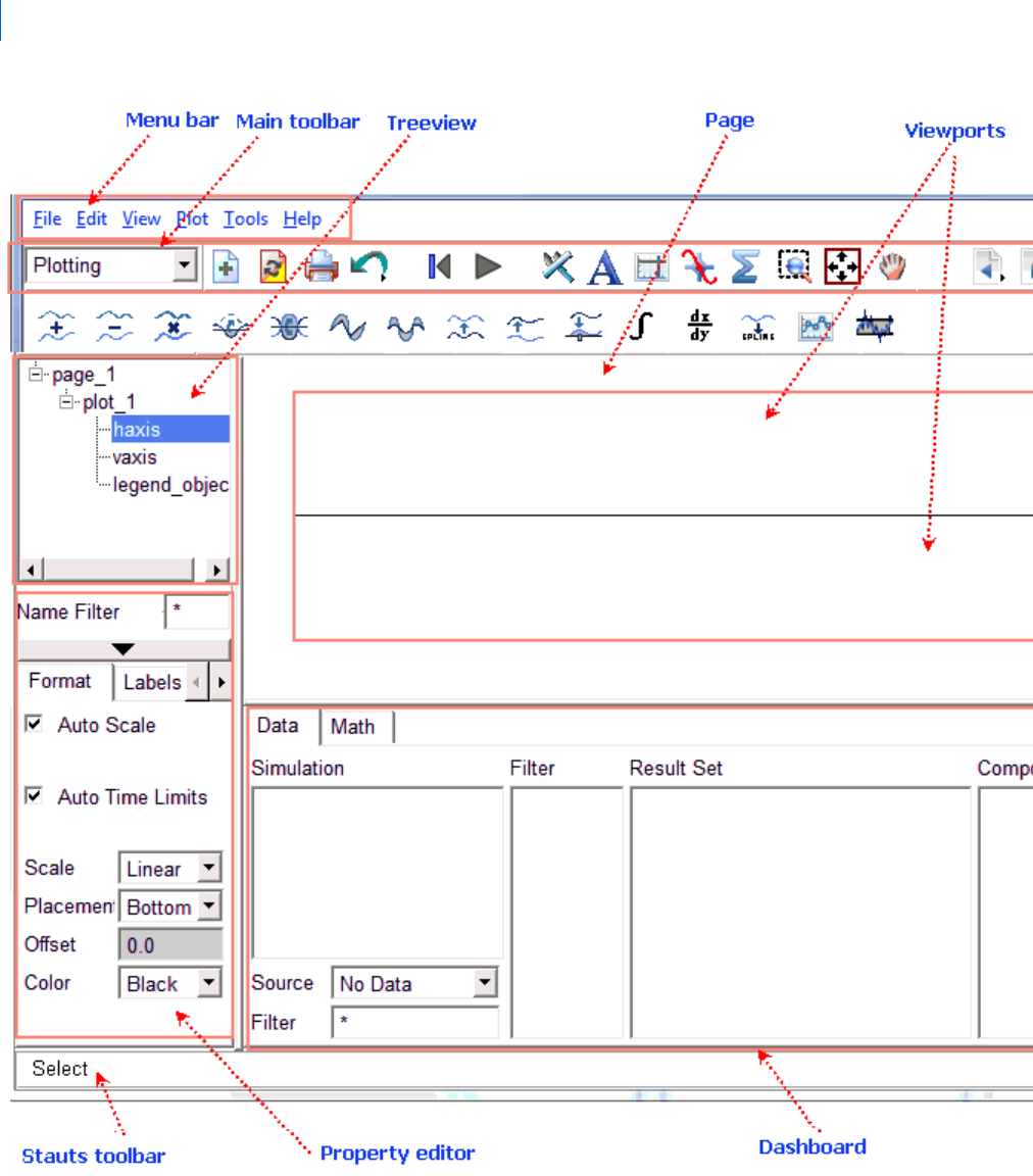
About the Adams PostProcessor Window
The following figure shows the Adams PostProcessor window. The elements shown are common to all modes.
Adams PostProcessor
Overview
4
Adams PostProcessor Window

5
Learning Adams PostProcessor Basics
Overview
Setting the Window Mode
Adams PostProcessor has four modes: animation, plotting, reports, and three-dimensional plotting (only
available with Adams Vibration data). Its mode changes depending on the contents of the current viewport
(see
Viewports). For example, the tools in the Main toolbar change if you load an animation. You can also
manually set the mode.
To switch modes manually
Do one of the following:
• Click in a viewport containing an animation, plot, or report.
• From the pull-down menu in the Main toolbar, select the desired mode.
• Right-click the viewport, and then select a Load command, such as Load Animation.
Managing Pages
Learn more about managing Pages.
Creating Pages
Renaming Pages
Displaying Pages
Displaying Headers and Footers on Pages
Creating Pages
To create a page:
From the View menu, point to Page, and then select New.
When you create a page, Adams PostProcessor automatically assigns a name to it.
Renaming Pages
To change the name of a page:
In the treeview, click the page to be renamed.
From the Edit menu, select Rename.
Enter the new name for the page.
Select OK.
Note: For information on deleting pages, see Deleting Objects.
Tip: From the Main toolbar, select .
Adams PostProcessor
Overview
6
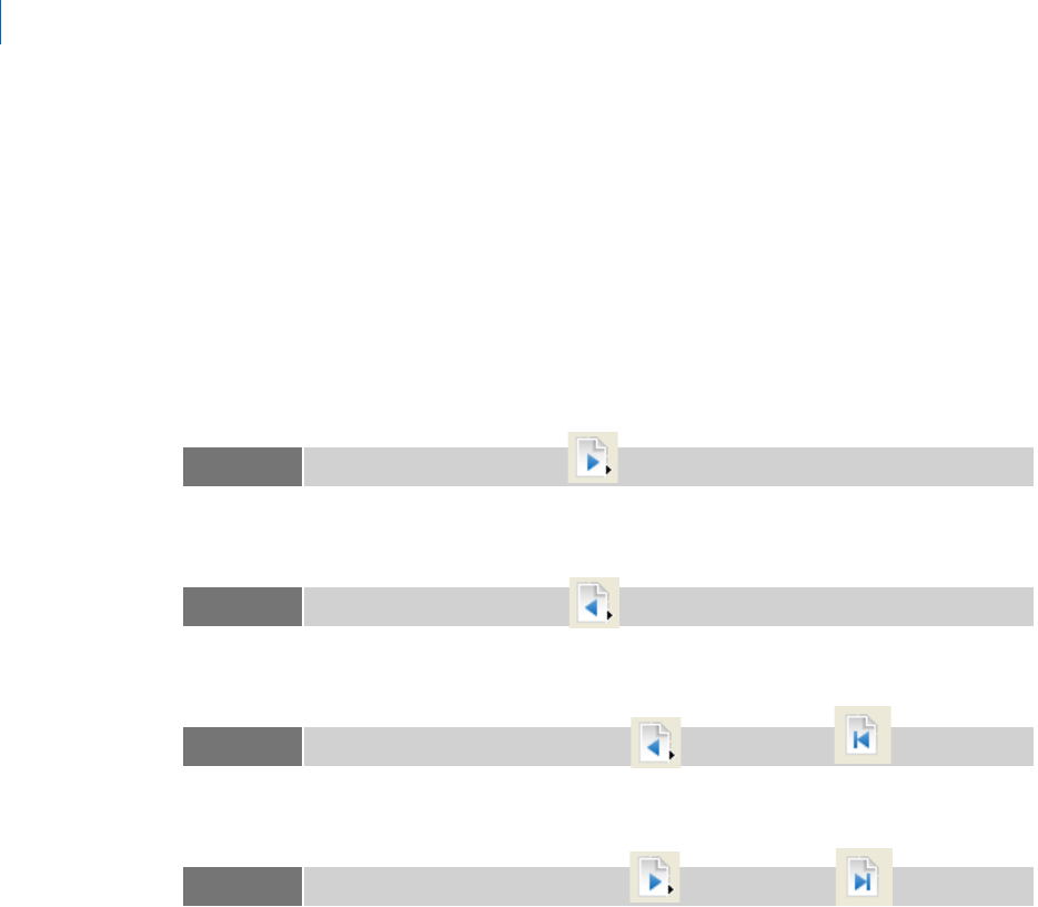
Displaying Pages
Adams PostProcessor provides you with several ways to move through the pages of plots.
To display a specific page, do one of the following:
In the treeview, click the page you'd like to display.
From the View menu, point to Page, and then select Display. From the list of pages, select the page
to display.
To navigate through the pages:
To display the next page, from the View menu, point to Page, and then select Next Page.
To display the previous page, from the View menu, point to Page, and then select Previous Page.
To display the first page, from the View menu, point to Page, and then select First Page.
To display the last page, from the View menu, point to Page, and then select Last Page.
Displaying Headers and Footers on Pages
You can display headers and footers on all pages. Each header and footer can have three items of information
(left, center, and right). Each item on the header footer can be a bitmapped image (.jpg, .xpm, or .bmp) or
text.
You can also set up default headers and footers to appear on all pages as explained in
PPT Preferences - Page.
To set up headers and footers on a page:
1. Select the page on which you want to display the headers and footers.
2. In the
Property Editor, select Header or Footer. Select None to turn off the display of headers and
footers.
3. Select the item of information (left, center, or right) that you are setting up.
4. Set Source to Text or Image and then:
Tip: From the Main toolbar, select .
Tip: From the Main toolbar, select .
Tip: From the Main toolbar, right-click and then select .
Tip: From the Main toolbar, right-click and then select .
7
Learning Adams PostProcessor Basics
About Data
• For text, enter the text to be displayed, and set the text font size and color.
• For an image, enter the location and name of the image file to be displayed, and the height at
which you want the image displayed.
Adams PostProcessor automatically displays the image as 50 pixels high.
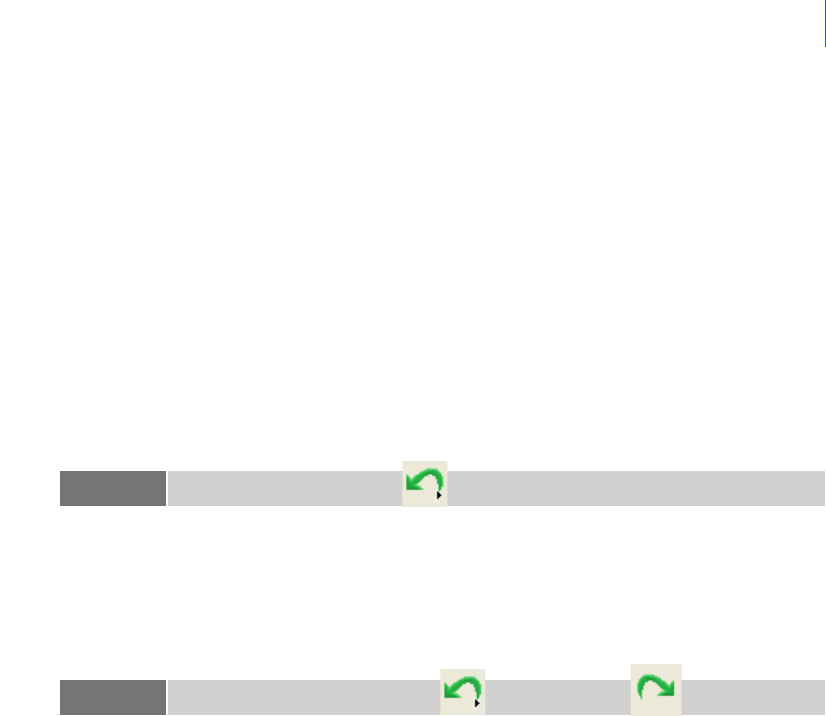
Undoing and Redoing Actions
You can undo the effects of most Adams PostProcessor commands. Adams PostProcessor remembers up to 10
operations, by default. Note that you cannot undo the effects of some commands, such as the commands in
the File menu.
To undo an operation:
On the Edit menu, select Undo.
If you change your mind and do not want to undo an operation, you can redo it.
To redo an operation:
On the Edit menu, select Redo.
Canceling Operations
You can cancel any operation that you started in Adams PostProcessor. For example, you can exit from a
dialog box or stop a Simulation or animation.
To cancel an operation, do either of the following:
Select the Cancel button on a dialog box if available.
Press the Esc key.
About Data
Creating Sessions and Adding Data
When you start Adams PostProcessor, it starts a new session file for you, called a notebook. To get results of
simulations into your notebook, you import the results. Once you've reviewed the simulation results, you can
save your notebooks, if Adams PostProcessor is in
Stand-alone mode, and you can export that data for use in
other programs.
Tip: From the Main toolbar, select .
Tip: From the Main toolbar, right-click , and then select .

Adams PostProcessor
About Data
8
Learn more about how to create notebooks, save your work, and import data:
Creating a New Session
Saving a Notebook
Adding Data
Creating a New Session
Each time you start Adams PostProcessor in Stand-alone mode, it creates a new session in which to work. You
can also create a new session at anytime.
To create a new session:
From the File menu, select New.
Saving a Notebook
In Stand-alone mode, Adams PostProcessor saves your current session in Notebooks. You can also save a copy of
a notebook with a different name or in a different location. When you save a notebook, Adams PostProcessor
saves all the pages you created and their content. It also saves the simulation results in the binary file. The
results are not associated with the files you imported.
To save an existing, named session:
From the File menu, select Save.
To save a new, unnamed session or to save a session with a new name:
1. From the File menu, select Save As.
2. Type a name for the notebook.
3. To save the document in a different directory, right-click the File Name text box, select Browse, and
then select the desired directory.
4. Select OK.
Adding Data
You can import data from the types of files shown below into Adams PostProcessor to animate, plot, or view
as a report. The data that you import appears at the top of the treeview.
Adams View command (.cmd). See Import - Adams View Command Files.
Adams Solver dataset (.adm). See Import - Adams Solver Dataset.
Adams Solver analysis (.req, .res, .gra). See Import - Adams Solver Analysis Files.
Adams Vibration results. See Importing Vibration Results.
Numeric data. See Import - Test Data.
DAC and RPC III. See Import - DAC or RPC III.
Wavefront objects. See Export - Wavefront.

9
Learning Adams PostProcessor Basics
Using Toolbars
Stereolithography and render. See Import - Stereolithography and Render Files.
Shell. See Import - Shell.
Reports. See Viewing Reports.
PPT Copy to Clipboard
1. To copy the contents of the entire page, right-click the page from the treeview and select Copy - To
Clipboard. Both the animation pane and the plot pane can now be pasted as a single image into
Word® or PowerPoint® (for example) by those applications’ “Paste” buttons or use Ctrl+V.
2. To copy the contents of an individual pane, select that pane by clicking in it and then right-click in
empty space on the given pane and select Copy - To Clipboard (or use keyboard shortcut Ctrl+C).
The content of that particular pane can now be pasted as a single image into Word® or PowerPoint®
(for example) by those applications’ “Paste” buttons or use Ctrl+V.
Exporting Data
You can export animation and plotting data in the following formats.
Spreadsheet format. See Export - Spreadsheet Data.
Numeric data. See Export - Numeric Test Data.
DAC and RPC III data. See Export - DAC or RPC III.
Tables (HTML or spreadsheet format). See Exporting Plots as Tables.
Reports (HTML). See Exporting Adams PostProcessor Data as an HTML Report.
Exporting Plots as Tables
To export plots as tables:
1. From the File menu, point to Export, and then select Table.
2. Type a name for the file.
3. Enter the name of the plot containing the data.
4. Select either html or spreadsheet.
5. Select OK.
Using Toolbars
The Adams PostProcessor window contains several toolbars that let you perform special functions.
Note: You can also record animations as AVI movies, TIFF files, and more. For more information,
see
Recording Animations.
Adams PostProcessor
Using Toolbars
10
Main toolbar - The Main toolbar appears by default. It contains tools for setting options and
performing operations. The contents of the toolbar change depending on the Adams PostProcessor
mode.
Curve Edit toolbar - Lets you manipulate curve data. See Displaying the Curve Edit Toolbar.
Statistics toolbar - Lets you view statistics about curves, such as the minimum and maximum values.
See
Displaying Plot Statistics About Curves.
Status bar - Displays information messages and prompts while you work. The right side of the status
bar displays the number of the displayed page and the total number of pages.
Learn more about the Main toolbar and how to display the different toolbars:
About the Main Toolbar
Setting Up and Displaying Toolbars
Using Tool Stacks
About the Main Toolbar
The Main toolbar appears at the top of the Adams PostProcessor window. It displays commonly used tools for
working with animations, plotting results, and
Reports. Some tools remain in all Modes, while other tools
change depending on the mode.
The following figures show groups of tools in the Main toolbar in different modes. You can display Tool tips
to see what a tool does.
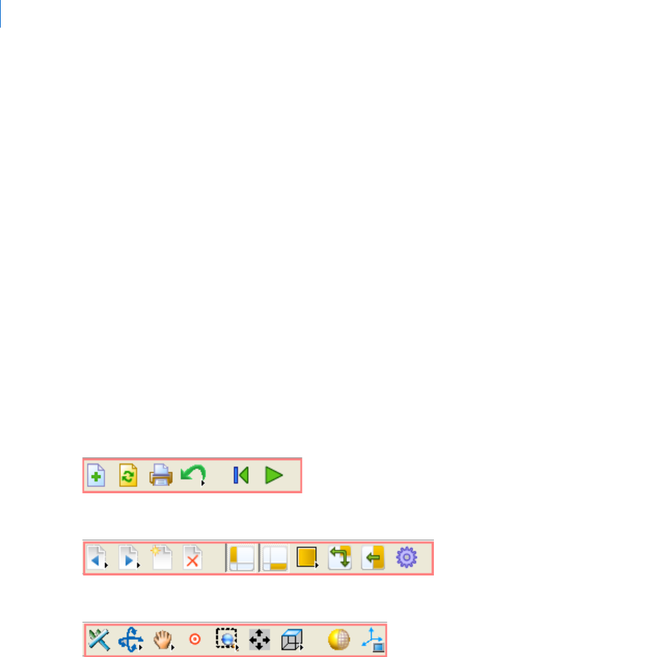
Main Toolbar Session Tools
Main Toolbar Page and Viewport Tools
Main Toolbar Animation Tools
11
Learning Adams PostProcessor Basics
Using Toolbars
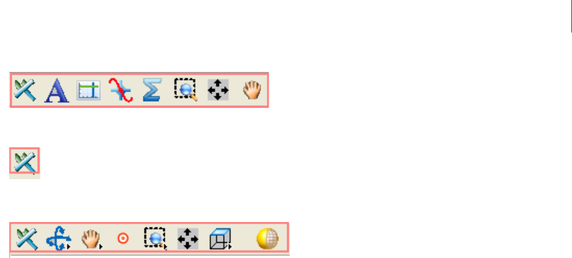
Main Toolbar 2D Plotting Tools
Main Toolbar Report Tools
Main Toolbar 3D Plotting Tools
Setting Up and Displaying Toolbars
You can turn the display of toolbars on and off. You can also set where the toolbars appear-either at the top
of the window under the menu bar or at the bottom of the window. You can also turn on and off the
dashboard and treeview. By default, the dashboard and treeview are displayed, the
Main toolbar appears at the
top of the window, the
Curve Edit and Statistics toolbars are turned off, and the status bar appears at the bottom
of the window.
To turn toolbars on or off:
From the View menu, point to Toolbars, and then select a toolbar.
To set the placement of toolbars:
1. From the View menu, point to Toolbars, and then select Settings.
The Toolbar Settings dialog box appears.
2. Select the visibility and placement of the items.
Your changes take place immediately.
Using Tool Stacks
In the Main toolbar, some of the tools are actually stacks of tools called tool stacks. The default tool or last
selected tool appears on top of the stack. A small triangle in the lower right corner of the top tool indicates
that there are more tools.
To select a tool from a tool stack:
1. Right-click a tool stack (a tool with a small triangle in the lower right corner).
2. Select the desired tool in the stack.
The selected tool now appears on top of the tool stack.

Adams PostProcessor
Interface Objects
12
Interface Objects
Setting Display of Interface Objects
You can turn on and off the display of the following interface objects:
Property Editor
Dashboard
Treeview
Toolbars (Learn about displaying toolbars)
To turn off the display of the property editor:
Click the down arrow at the top of the property editor. See Picture of Property Editor Down Arrow.
To turn on the display of the property editor:
Click the up arrow. See Picture Property Editor Up Arrow.
To toggle the display of the dashboard or treeview:
From the View menu, point to Toolbars, and then select Dashboard or Treeview.
Resizing and Resetting Interface Objects
You can adjust the size of the different interface objects:
Property Editor
Dashboard
Treeview
Toolbars
For example, you can increase the height of the dashboard so you can see more results.
To change the size of an interface object:
1. Point to a border of the interface object that you want to resize.
2. When the cursor changes to a double-sided arrow, drag the cursor until the object is the desired size.
To set the objects back to their original dimensions:
From the View menu, select Reset GUI Dimensions.
Tip: To turn off the dashboard, on the Main toolbar, select .
To turn off the treeview, on the Main toolbar, select .

13
Learning Adams PostProcessor Basics
Managing Viewports
Managing Viewports
You can change the layout of a Page and place up to six Viewports on a page. Adams PostProcessor provides
you with 12 viewport layouts from which you can choose.
Learn more about setting up viewports on pages:
Setting the Viewport Layout
Selecting a Viewport
Expanding Viewports
Swapping Viewport Contents
Clearing Viewports
Setting the Viewport Layout
You select the Page layout you'd like from a palette of layouts or from the Page Layout tool stack on the Main
toolbar
. The palette and tool stack contain the same set of viewport layouts. If you select to display the palette,
you can keep it open so that you can quickly select another layout.
To select a layout:
1. Do either of the following:
• On the View menu, point to Page, and then select Page Layouts.
• On the Main toolbar, right-click the Page Layout tool stack .
A selection of layouts appears.
2. Select a layout.
3. If you used the palette, select Close to close. You can, however, keep the palette open and continue
with your work so you can quickly change your window layout.
Selecting a Viewport
By default, Adams View changes the display of the active viewport, leaving the other Viewports the same. The
active viewport is outlined in red.
Note: You can also set the orientation of an animation in a viewport. See Controlling the Animation
Display
Note: A page that contains an FFT or Bode plot has two viewports. For an FFT plot, the top
viewport contains the plot with the input data and the bottom viewport contains the plot
with the output from the FFT. For a Bode plot, the top viewport contains the gain plot and
the bottom viewport contains the phase plot.
Adams PostProcessor
Managing Viewports
14
To activate viewport so that any display changes occur in it:
Click anywhere in the background of the viewport. Be sure the border changes to red.
Expanding Viewports
You can quickly zoom in on a viewport by expanding it to the full window.
To quickly zoom in on just one of the viewports:
1. Click the viewport you want to zoom in on.
2. On the View menu, select Expand View.
To return to viewing all the viewports on the page:
On the View menu, select Expand View again.
Swapping Viewport Contents
You can swap the contents of one viewport (see Viewports) with the contents of another viewport. The
viewports do not have to be on the same
Page.
To swap the contents of viewports:
1. Select the viewport to be used as the default.
2. On the View menu, select Swap View.
3. Select the window whose contents will be swapped with the first viewport you selected.
Clearing Viewports
You can remove all objects in a viewport.
To clear a viewport:
1. Select the viewport to be cleared.
2. On the View menu, select Clear View.
Using Shortcut Menus
The different types of Shortcut menus are explained in the table below.
Tip: From the Main toolbar, select .
Tip: From the Main toolbar, select .
15
Learning Adams PostProcessor Basics
Managing Viewports
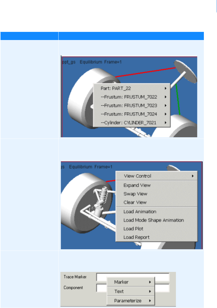
When cursor is over: The shortcut menu lets you:
Modeling object in the
viewport (for example, a
rigid body). See
Viewports.
Select and display information about the object.
Viewport (over no
modeling or plotting
object)
Set the display of the viewport, such as zoom in or change the view
orientation.
Text box in a dialog box,
Property Editor, or Dashboard
Enter information required in the text box, such as lets you browse for
a file or paste text in the file.

Adams PostProcessor
Using the Treeview
16
Using the Treeview
Learn about using the Treeview:
Expanding and Collapsing the Contents of the Objects
Setting Up Highlighting
Filtering the Treeview
Sorting the Treeview
Expanding and Collapsing the Contents of Objects in the Treeview
To see the contents of an object in the Treeview:
Click the plus sign (+) in front of the object.
To see the contents of all objects in the treeview:
Right-click the treeview, and then select Expand All.
To collapse the contents of an object in the treeview:
Click the minus sign (-) in front of the object.
To collapse the contents of all objects in the treeview:
Right-click the treeview, and then select Collapse All.
Setting Up Highlighting of Treeview Objects
You can set up the treeview so that whenever you highlight an object in the treeview, Adams PostProcessor
also selects it on the page and the reverse. Highlighting is on by default.
To toggle highlighting:
Right-click the treeview, and select Toggle Highlighting.
Filtering the Treeview
You can filter the objects in the treeview so only objects of a specified name or object type appear. For
example, you can display only geometry, curves, or animations. By setting filters in the treeview, you can
quickly modify a group of common objects. By default, Adams PostProcessor displays all types of objects. (See
the
example.)
To filter objects based on their names:
Below the treeview, in the Name Filter text box, enter the name of the object or objects that you
want to display. Enter any wildcards that you want included. See Tips on Entering Wildcards.

17
Learning Adams PostProcessor Basics
Using the Treeview
To filter objects based on their type:
Right-click the treeview, point to Type Filter, and then select the type of object that you want to
display.
To reset the filter to show all plotting or modeling objects:
Right-click the treeview, point to Type Filter, point to Plotting or Modeling, and then select All.
To reset the filter to show all types of objects:
Right-click the treeview, point to Type Filter, and then select All.
To select all objects of a particular type:
1. Filter the objects in the treeview so it displays only objects of a particular type.
2.
Expand all objects in the treeview.
3. Right-click the treeview, and select Select All.
Example
Changing the properties of the horizontal axis limits of all plots in your session would be tedious if you had
to access each plot individually. The treeview filter makes this much easier.
To use the treeview filter to change axis limits:
1. Set the type filter so only plot axes are displayed.
2. Right-click the treeview, point to Type Filter, point to Plotting, and then select Axis.
3. Right-click the treeview, and select Expand All.
The treeview expands to display all axes.
4. At the bottom of the treeview, in the Name Filter text box, enter h* to display only horizontal axes.
5. Right-click the treeview, and select Select All Axes.
6. In the Property Editor, change the values for the axes. For example, clear the selection of Automatic
and set upper and lower limits.
Sorting the Treeview
You can sort the objects in the Treeview by name and type. The default is to sort in the order they are stored
in the Modeling database.
To sort objects:
Right-click the treeview, point to Sort By, and then select the type of sort.
Adams PostProcessor
About Objects
18
About Objects
Selecting and Deselecting Objects
You can select any object in the Treeview or in a viewport (see Viewports). When you select objects in Adams
PostProcessor, they appear highlighted in both the viewport and the treeview. You can turn off the
highlighting as explained in
Setting Up Highlighting. You can also deselect all objects at once.
To select objects in the treeview or screen:
Click the object using the Select tool .
To select multiple objects:
To select a single object, click the object using the left mouse button.
To select a continuous set of objects, you can:
• Drag the mouse over the objects that you want to select or click on one object, hold down the
Shift key, and click the last object in the set. All objects between the two selected objects are
highlighted.
• Click on the first object, hold down the Shift key, and then use the up or down arrow to select a
block of objects.
To append to the list of selected objects, hold down the Ctrl key, and click the objects. You can do
this in either the treeview or a viewport.
To remove objects from the selected list, hold down the Ctrl key, and click the selected object.
In treeview, you can also select all objects of a particular type. For more information, see
Filtering the Treeview.
To deselect objects:
From the Edit menu, select Deselect All.
Renaming Objects
To rename an object displayed in the treeview:
1. In the Treeview, select the object you want to rename.
2. Either:
• On the Edit menu, select Rename. Type the new name, and then select OK.
• Click the object again. Type the new name, and then press Enter.
Tip: Ctrl + D.

19
Learning Adams PostProcessor Basics
About Objects
To rename any object:
1. From the Edit menu, select Rename.
2. Click the More button to display a list of objects.
3. Select an object. Double-click an object with a + in front of it to see more objects.
4. Select OK.
5. Type the new name, and then press OK.
Deleting Objects
You can delete any objects selected in the treeview. In addition, you can use the Database Navigator to find
an object to delete.
Adams PostProcessor deletes the contents of an object when it deletes the object. For example, Adams
PostProcessor deletes the plots on a page when you delete the page.
To delete selected objects:
1. Select the objects that you'd like to delete. Use the Treeview to make the selection easy.
2. From the Edit menu, select Delete.
To delete an object through the Database Navigator:
1. Clear any selection of objects.
2. From the Edit menu, select Delete.
3. Use the Database Navigator to find the object you'd like to delete, and then select OK.
Printing Plots, Animations, and Reports
You can print Pages directly to a printer or store them in a file for printing at a later time.
Tip: To delete a page, from the Main toolbar, select .
Notes: Adams PostProcessor only prints the portion of a report or table that fits on the paper.
To print a multi-page report, open the report in a browser and print from there.
To print a multi-page table, export the table in HTML format, open the report in a
browser, and print from there. For information on exporting a table as HTML, see
Exporting Data.
Adams PostProcessor
About Objects
20
Pages with only reports and tables on them print significantly faster than pages with mixed views (for
example, plot and report), depending on the type of printer being used.
To print pages:
1. On the File menu, select Print.
The Print dialog box appears.
2. Set the printing options as shown in the table below and select OK.
To cancel printing:
Select Cancel or press the Esc key.
Tip: On the Main toolbar, select .
To print: Do the following:
To a p r i n t e r On Linux, in the Print to area, select Printer and enter an operating system
command to execute the print job (for example, lpr -Psp2 or lp -c -Ppd1).
On Windows, select also show Windows print dialog box to display the
default Windows printer dialog box from which you can select a printer. The
dialog box appears after you select OK.
Only to a file In the Print to area, select File and enter the location and name of the file to which
you want to print the page.
Note that if you print more than one page to a file, Adams PostProcessor uses the
page number of each page as the name of the file.
In a different format If you selected to print to a file, select the type of file format. You can select BMP,
XPM, JPG, TIFF and PNG.
Note: If you select jpg format, you can set the level of quality.
In color or black and
white
Select either Black and White or Color. If you select Black and White, Adams
PostProcessor prints all colors in black and the background in white even if you
are using a color printer.
Selecting black and white is generally considered more readable for presentations,
but you should use altering line style or line thickness to distinguish between the
curves on the plot.
If you print a plot in color but send it to a black-and-white printer, the printer
approximates the colors using grayscale.
21
Learning Adams PostProcessor Basics
Using Wildcards
Using Wildcards
You can use wildcards to narrow any search, set the type of information displayed in a window, such as the
Database Navigator, or specify a name of an object in a dialog box.
Listing of Wildcards
Tips on Entering Wildcards
Here are some tips for entering wildcards:
Case is insignificant so xYz is the same as XYz.
You can match alternative sequences of characters by enclosing them in braces and separating them
with commas. For example, the pattern a{ab,bc,cd}x matches aabx, abcx, and acdx.
You can form character sets that match a single character using brackets [ ]. For example, [abc]d
matches ad, bd, and cd.
You can use a dash (-) to create ranges of characters. For example, [a-f1-4] is the same as
[abcdef1234].
You can use a backslash (\) to include a special character as part of the character set. For example,
[ab\]cd] includes the five characters a, b, ], c, and d.
Here are some examples of more complex patterns and possible matches:
At a different
orientation
Select the type of orientation: Landscape or Portrait.
On a different size
paper
Select the size of paper or, to accept the current default paper for the printer, select
Default.
A particular page or
range of pages
Select to print the current page, all pages, or a range of pages.
To print: Do the following:
This character: Matches:
* (asterisk) Zero or more characters
? Any single character
[ab] Any one of the characters in the brackets
[^ab] Any character other than the characters following the caret symbol (^) in the
brackets
[a-c] Any one character in a range enclosed in brackets
{ab, bc} Any of the character strings in the braces

Adams PostProcessor
Using Wildcards
22
x*y - Matches any object whose name starts with x and ends with y. This would include xy, x1y, and
xaby.
x??y - Matches only those objects with four-character long names that start with x and end with y.
This would include xaay, xaby, and xrqy.
x?y* - Matches all of those objects whose names start with x and have y as the third character. This
would include xayee, xyy, and xxya.
*{aa,ee,ii,oo,uu}* - Matches all those objects whose name contains the same vowel twice in a row.
This would include loops and skiing.
[aeiou]*[0-9] - Matches any object whose name starts with a vowel and ends with a digit. This would
include eagle10, arapahoe9, and ex29.
[^aeiou]?[xyz]* - Matches any object whose name does not start with a vowel and has x, y, or z as the
third letter. This would include thx1138, rex, and fizzy

1
Animating Results
Animations Basics
Animating Results
Animations replay the frames calculated during a Simulation in other Adams products. Animations are
helpful for understanding the behavior of the entire physical system, providing an important context to xy
plotting.
When you load an animation or set the Adams PostProcessor mode to animation, Adams PostProcessor
changes its interface to allow you to play and control animations. See
Modes.
Animations Basics
Types of Animations
You can load two types of animations in Adams PostProcessor:
Time-domain animations
Frequency-domain animations (referred to as normal-mode animations in Adams Vibration)
About Time-Domain Animations
When you perform a time-based simulation in an Adams product, such as a dynamics simulation in Adams
View, Adams Solver creates one animation frame for every output step that you request in the simulation. For
example, if you performed a simulation from 0.0 to 10.0 seconds and asked for output every 0.1 seconds,
Adams Solver records data at 101 steps or frames. It creates a frame every tenth of a second for ten seconds
plus one at time 0.0.
About Frequency-Domain Animations
Using Adams PostProcessor, you view your model oscillating at one of its natural frequencies. It cycles
through the model deformation starting from the operating point of the requested natural frequency of the
eigensolution. You can also see the effect of the damping on the model and display a table of eigenvalues.
When you perform a linear simulation of your model, Adams Solver linearizes the model at an operating
point you specify and calculates the eigenvalues and eigenvectors. Adams PostProcessor then uses the
information to display the animated deformed shape as predicted from the eigensolution. Because the linear
solution eigenvectors are normalized, you can specify what the maximum amount the animated deformed
shape should translate or rotate to get a meaningful animation or recognizable shape.
The animation frames correspond to pictures of the model interpolated between the maximum deformation
in the positive and negative directions. The animation then cycles through the deformation of the model
mode shape, from undeformed, to maximum deformed, to negative maximum deformed, and finally to the
Note: If you are using Adams Vibration with your Adams product, you can also use Adams
PostProcessor to view forced-vibration animations. For more information, see the
Adams
Vibration online help
.

Adams PostProcessor
Animations Basics
2
undeformed shape. This deformation is about the operating point of the requested natural mode of the
eigensolution.
You can only animate periodic and aperiodic eigenmodes (that is, modes with an imaginary component of
the eigenvalue = 0). However, when animating aperiodic modes, Adams PostProcessor warns you that the
node has no oscillatory motion.
Loading Animations
To play an animation with Adams PostProcessor in Stand-alone mode, you must import the necessary files or
open an existing notebook file (.bin) (see
Notebooks) and then load the animation. If you are using Adams
PostProcessor with an Adams product, such as Adams View, the necessary files are available in Adams
PostProcessor after you run an Interactive Simulation or event. You only need to load the animation.
For Time-domain animations, you must import a Graphics file (.gra) containing the animation. The
graphics file is created by another Adams product, such as Adams View or Adams Solver.
For Frequency-domain animations, you must import the Adams Solver dataset files (.adm) and Results
file (.res) from a simulation.
To import animations:
From the File menu, select Import, and then import the necessary files.
Learn more about
Adding Data
To load an animation in a viewport:
Right-click the background of a viewport (see Viewports), and select:
• Load Animation for a time-domain animation.
• Load Mode Shape Animation for a frequency-domain animation.
Playing Animations
When you play Time-domain animations, Adams PostProcessor plays every frame by default, as rapidly as
possible. By default, it also continues to play through the animation, until you stop it. You can also set the
animation to play only once or play first forwards and then backwards.
To play an animation:
From the Dashboard or Main toolbar, select .
To play an animation backwards:
From the dashboard, select .
3
Animating Results
Animations Basics
To play an animation one frame at a time:
From the dashboard, next to the slider, click the right and left arrow buttons.
To pause an animation:
From the dashboard, select .
To reset the animation to the beginning:
From the dashboard, select .
To set the animation play options, in the dashboard, set Loop to:
Forever - Continuously loop through the animation.
Once - Animate one time.
Oscillate - First play the animation forwards and then play it backwards (for example, in a 100-
frame animation, animate from 1 to 100 then back from 100 to 1).
Oscillate forever - Oscillate forward and backward repeatedly.
Recording Animations
You can record an animation as a series of files, each containing one frame of the animation. Adams
PostProcessor saves the files to your current working directory. Once you've recorded the animation, you can
import the images into a third-party multimedia tool to create movies.
Before recording the animation, you can:
Select the format: .avi, .tif, .jpg, .bmp, .mpg, .png, and .xpm (.avi format is only available on
Windows).
Define the area of the viewport to record (see Viewports).
Set the prefix used to name the set of files. Adams PostProcessor appends a unique number to the
prefix to form the name of each file. For example, if you specify a prefix of suspension, then each .tif
file is named suspension_0001.tif, suspension_0002.tif, and so on. If you do not specify a name, the
prefix is frame (for example, frame_001.tif).
For .avi format, set the frame rate, turn off compression to improve the quality of the images, and set
the interval between key frames. The default is compression with each key frame 5000 frames apart.
For .mpg format, set options for ensuring the viewing in different playback programs.
Tip: Configuring Browser to Play MPEG Video.
Running MPEG Movie Using Windows Media Player .
Adams PostProcessor
Animations Basics
4
To record an animation:
From the dashboard, select , and then select .
To set recording options:
1. From the dashboard, select Record.
2. Select the type of file format in which to save the frames.
3. In the Filename text box, enter the name you want Adams PostProcessor to use as the prefix of each
file it creates.
4. To define an area of the viewport to record, select Frame Size, and then enter the size in the Width
and Height text boxes. If the frame size exceeds the area currently on the screen, a warning message
appears. You can fit the frame on the screen by resizing the dashboard, hiding toolbars, or increasing
the size of the Adams PostProcessor window. See Resizing and Resetting Interface Objects.
5. If you selected:
• AVI format, set the number of frames per second, the compression, if any, and the interval
between key frames.
• MPG format, set either of the following:
Notes: When a digital movie stream is encoded with compression, the pixels of each frame are
evaluated against previous frames (those designated as key) and only pixels that
changed are stored. For example, a movie of a car traveling along a road can have many
pixels in the image background that do not change during the entire movie. Therefore,
storing only the pixels that change allows for significant compression. In many cases,
however, it can degrade movie quality, especially with movies where a large percentage
of pixels are changing from frame-to-frame, such as with wireframe graphics. Because
Adams PostProcessor lets you set the key frames rates, you control both the
compression factor and the movie quality.
Movies with many key frames will have high quality, while movies with few key frames,
such as the default every 5000 frames, will have lower quality. For a typical 20-second
.avi movie of a shaded Adams model, a key frame rate would be 12.
Note: When you set use compression when recording in AVI format, the playback program
may restrict the size of image frames, usually to a multiple of 2 or 4. Therefore, your
recording may appear cut off on one or more sides. The workaround is to change the
animation window size before recording.

5
Animating Results
Animations Basics
Compress the file using P frames - Turning off the compression using P frames ensures your
movie plays in many playback programs, including as xanim. It results, however, in a much larger
file (up to 4 times as large).
Round size to multiples of 16 - Some playback programs require the pixel height and width to
be multiplies of 16. Turning this option on ensures that you movie plays in many playback
programs.
Configuring Browser to Play MPEG Video
In Windows, use Windows Media Player.
For Linux try mtv or SMPEG or all the software derived from SMPEG.
Enter the command to launch your MPEG player. For example on an SGI, you would launch 'movieplayer'
by entering the command:
/usr/sbin/movieplayer -nofork %s
Running MPEG Movie Using Windows Media Player
When running a MPEG movie using Windows Media Player in Internet Explorer, you may receive the
following error message:
Internal MPEG Error, Code 3
You must be logged in as administrator when opening the .mpg file and running the Windows Media Player
to install mpeg codedc, which is required to run .mpg files.
For more information, see the Microsoft Support Web pages.
Overlaying Animations
You can play one animation on top of another animation. To help you see the two animations, you can change
their color and offset one from the other. You'll find this helpful when you want to visually compare the
results of two or more modeling changes.
To overlay animations:
1. From the Dashboard, select Overlay.
2. From the list, select the animations to be overlayed.
3. In the Offset text box, enter the amount by which to offset the animations. Enter the x, y, and z
values. Adams PostProcessor applies the offset to each animation if you selected more than two
animations to overlay.
4. In the Colors text box, enter the colors in which to display the overlaid animation.
Tips on
Entering Object Names in Text Boxes.

Adams PostProcessor
Controlling Time-Domain Animations
6
Displaying Part Information
To display part information:
1. Press and hold down the Ctrl key.
2. Move the cursor over the animation.
Adams PostProcessor displays part information.
Controlling Time-Domain Animations
Learn how to control Time-domain animations:
Playing Portions of a Time-Domain Animation
Setting Animation Speeds in Time-Domain Animations
Displaying Specific Frames in Time-Domain Animations
Tracing the Paths of Points in Time-Domain Animations
Superimposing Frames in Time-Domain Animations
Setting Trailing of Frames
Playing Portions of a Time-Domain Animation
By default, Adams PostProcessor uses every frame of a time-domain animation. You can select to skip any
number of frames and play only a portion of the animation based on time or frame number. For example, to
view an animation between 3.0 and 5.5 seconds, you would set the start time to 3.0 and the end time to 5.5.
To skip frames:
1. From the Dashboard, select Animation.
2. In the Frame Increment text box, enter the number of frames to skip.
3.
Play the animation.
To play only a portion of the animation:
1. From the dashboard, select Animation.
2. Set Display Units to Frame or Time.
3. In the Start text box, enter the starting frame or time and in the End text box enter the ending frame
or time.
4.
Play the animation.
Note: Each animation you overlay must have the same beginning, increment and end times.

7
Animating Results
Controlling Time-Domain Animations
Setting Animation Speeds of Time-Domain Animations
You can change the speed at which time-domain animation play by introducing a time delay between each
frame of an animation. Use the slider on the
Animation Dashboard to introduce the delay. The default, when the
slider is all the way to the right, is to play each animation as fast a possible. Moving the slider to the left
introduces a time delay of up to 1 second.
To change the speed:
1. From the Dashboard, select Animation.
2. Click and drag the Speed Control slider at until you reach the desired time delay.
Displaying Specific Frames of Time-Domain Animations
Adams PostProcessor provides you with several options for playing specific frames of Time-domain animations.
You can play one frame, display each frame one at a time, or display a frame associated with a particular time.
You can also display a frame or frames representing:
Model input - Model input represents the state that the model is in before the simulation. It does
not account for assembly initial conditions or static solutions.
Static equilibrium
Contact between parts - By default, Adams PostProcessor does not display intermittent contact
frames that two- and three-dimensional contacts produce to avoid the illusion of deceleration during
animations.
To display a frame from an animation:
1. From the Dashboard, select Animation.
2. Do one of the following:
• Click and drag the topmost slider until you reach the number of the frame or time you want to
display.
• In the text box to the right of the slider, enter the number of the frame or time you want displayed.
To display the frame representing the model input:
1. From the dashboard, select Animation.
2. Select Model Input.
To display the frames representing static equilibrium:
1. From the dashboard, select Animation.
2. Select Include Static.
3. Continue selecting Next Static to view all static equilibrium positions.

Adams PostProcessor
Controlling Time-Domain Animations
8
To display the frames representing contacts:
1. From the dashboard, select Animation.
2. Select Include Contacts.
3. Continue selecting Next Contact to view all contacts between parts.
Tracing the Paths of Points in Time-Domain Animations
During Time-domain animations, you can draw curves on the screen that represent the path that one or more
points in your model travelled. This can be useful when you are trying to design a mechanical system to
produce a certain motion, and want to see whether or not the parts move as intended.
Tracing the paths of points can also be useful when performing envelope studies to see if any parts move
outside a particular working envelope as the mechanical system completes a typical work cycle. By default,
Adams PostProcessor does not trace the paths of any points in your model during animation.
To draw paths on the screen, you specify one or more Markers for which you want paths generated. Adams
PostProcessor draws curves representing the path of the marker during each animation frame.
To trace the paths of points during an animation:
1. From the Dashboard, select Animation.
2. In the Trace Marker text box, enter the names of one or more markers for which you want Adams
PostProcessor to generate paths.
Tips on
Entering Object Names in Text Boxes.
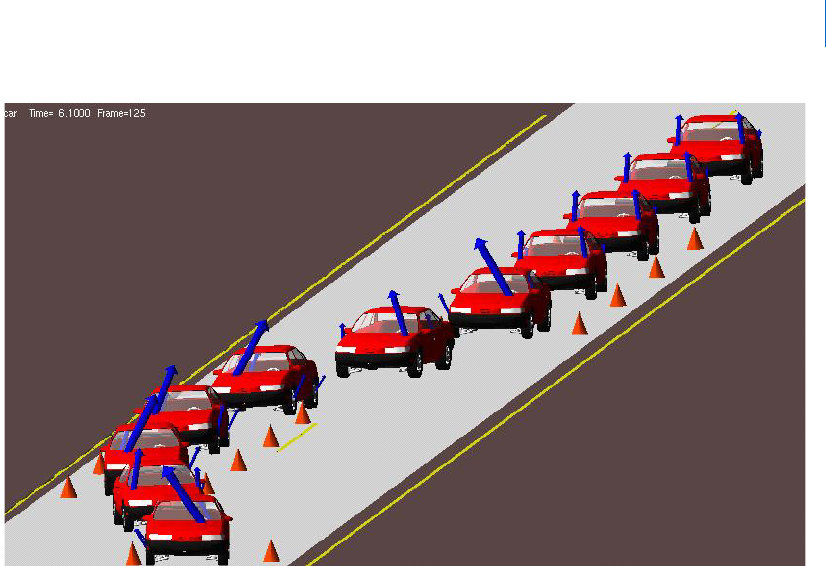
Superimposing Frames
You can superimpose successive frames of Time-domain animations. When you toggle the Superimpose button,
Adams PostProcessor accumulates each frame, as shown below.
9
Animating Results
Controlling Time-Domain Animations
To superimpose frames:
1. From the Dashboard, select Animation.
2. Select Superimpose.
3.
Play the animation.
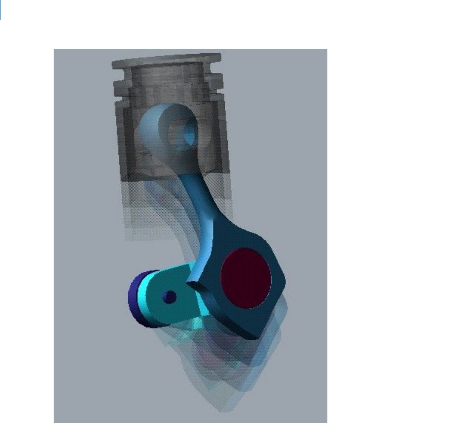
Setting Trailing Frames in Time-Domain Animations
You can overlap successive frames of Time-domain animations. Setting up trailing of frames helps you to better
visualize the motion of a model or to add a sense of motion to still images of the animation.
You can control the decay rate using the Trail Decay Rate slider. It sets the rate at which the frames disappear.
By default, the slider is all the way to the left, specifying no decay.
Adams PostProcessor
Controlling Frequency-Domain Animations
10
To trail frames:
1. From the Dashboard, select Animation.
2. In the Trail Frames text box, enter the number of frames to trail.
3. Move the Trail Decay Rate to set the rate at which the frames diminish or decay.
4.
Play the animation.
Controlling Frequency-Domain Animations
Learn how to control Frequency-domain animations:
Displaying Specific Modes or Frequencies for Frequency-Domain Animations

11
Animating Results
Controlling Frequency-Domain Animations
Controlling the Number of Frames Per Cycle
Setting Linear Mode-Shape Display for Frequency-Domain Animations
Viewing Eigenvalues for Frequency-Domain Animations
Displaying Specific Modes or Frequencies of Frequency-Domain
Animations
You can select to view a specific mode or frequency in your frequency-domain animation.
To select to view a mode or frequency:
1. From the Dashboard, select Mode Shape Animation.
2. Set the pull-down menu to either:
• Mode and enter the number of the mode to be viewed. You can also use the +/- buttons to move
through the modes.
• Frequency and enter the frequency of the mode to be viewed.
If you specify the frequency, Adams PostProcessor uses the mode closest to the specified
frequency. If you specify neither the mode nor the frequency, Adams View deforms the model
using the first mode.
3.
Play the animation.
Controlling the Number of Frames Per Cycle
For a linear mode-shape animation, you can control the number of frames per cycle. Adams PostProcessor
performs the interpolation between the frames using trigonometric functions; therefore, the frames tend to
be segregated at the maximum deformation in the positive and negative directions.
To set the number of frames per cycle:
1. From the dashboard, select Mode Shape Animation.
2. In the Frames Per Cycles text box, enter the number of frames to be displayed for each cycle.
3.
Play the animation.
Note: To view the modes in the eigensolution to see which you should use, see Viewing
Eigenvalues
.
Note: A full cycle goes from undeformed, to maximum positive displacement, back to undeformed,
then to maximum displacement in the negative direction, and finally back to undeformed.
Adams PostProcessor
Controlling Frequency-Domain Animations
12
Setting Linear Mode-Shape Display for Frequency-Domain Animations
When you run Frequency-domain animations, you can:
Set scale factor - You can specify the amount parts translate or rotate from their undeformed
position. If you do not specify a scale factor, Adams PostProcessor translates parts no more than 20
percent of model size and 20 degrees.
Show time decay - You can specify whether the amplitudes of the deformations are to remain
constant or decay due to the damping factor calculated in the eigensolution.
Superimpose the modes - You can select to show each mode superimposed on the other modes.
Show undeformed model - You can set whether Adams PostProcessor displays the undeformed
model with the deformed shape superimposed on top of it. If you select to show the undeformed,
you can select a color for the undeformed model. If you do not specify a color, Adams PostProcessor
displays the undeformed model using the same color as the deformed mode.
To set the frequency-domain control display:
1. From the dashboard, select Mode Shape Animation.
2. If desired, select any of the options shown in the table below.
3.
Play the animation.
Frequency-Domain Animation Display Options
Viewing Eigenvalues for Frequency-Domain Animations
You can display information about all an eigensolution's predicted eigenvalues in the Information Window
for
Frequency-domain animations. Once you display the information in the Information window, you can save
it to a file.
The information includes:
Mode number - Sequential number of the mode that the eigensolution predicted.
Frequency - Natural frequency corresponding to the mode.
Damping - Damping ratio for the mode (the log decrement is another way to represent this
quantity).
To: Do the following:
Set the amount parts
translate or rotate from their
undeformed position
Enter the scale in the Scale Factor text box.
Show time decay Select Show time decay.
Superimpose modes Select Superimpose.
Show undeformed mode Select Show undeformed and then, in the Color text box, enter a color.
Tips on
Entering Object Names in Text Boxes.

13
Animating Results
Controlling the Animation Display
Eigenvalues - List the real and imaginary part of the eigenvalue.
To view eigenvalues:
1. From the Dashboard, select Mode Shape Animation, and then select Table of Eigenvalues.
The Information window appears.
2. After viewing the information, select Close.
Controlling the Animation Display
You can set many options for how animations appear on the screen:
Setting the View of Your Animation
Setting Display of Screen Icons
Setting Display of Triad
Changing Part Display
Zooming the Display
Fitting the Display
Setting the Center of a Viewport
Setting the View Perspective
Setting Rendering Mode of Animations
Specifying the Camera Perspective
Setting Lighting
Setting the View
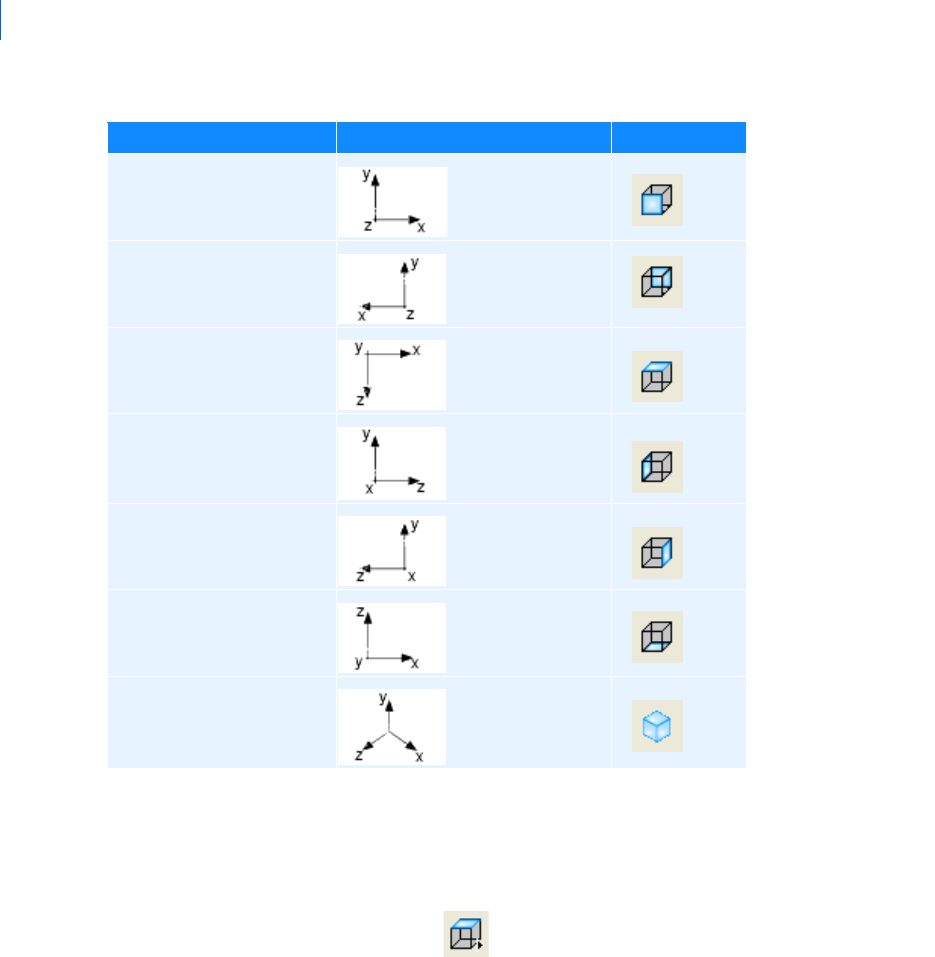
Adams PostProcessor provides seven standard views of your animation or three-dimensional plot that you can
display. The table below lists the views, their coordinate system orientations, and the tools on the
Main toolbar
that activate them. You can also redefine the orientations as explained in
PPT Preferences - Orientation.
Standard Views
Adams PostProcessor
Controlling the Animation Display
14
To set a view in a viewport:
1. Click the viewport you want to change.
2. Do one of the following: |
• On the View menu, point to Pre-Set, and then select a view.
• On the Main toolbar, right-click , and then select one of the View Orientation tools.
Setting Display of Screen Icons
By default, Adams PostProcessor turns off all Screen icons during animations to speed up the animation.
Displaying icons can be very helpful when debugging your model. For example, displaying screen icons
during animations allows you to see if joints or forces applied to parts are behaving as expected because you
can see their icons move as the animation progresses. Displaying screen icons can also help you see how
coordinate system markers move during animations because they control the locations and directions for
constraints and forces.
You can display the: The default orientation is: Its tool is:
Front
Back
To p
Left
Right
Bottom
Isometric
15
Animating Results
Controlling the Animation Display
Note that if you import your animation through a Graphics file (.gra) only, you do not have joint or force
icons.
You can also control the visibility of the part coordinate triad and the center of gravity marker as explained
in
PPT Preferences - Animation.
To display screen icons during an animation:
1. From the dashboard, select View.
2. Select Display Icons.
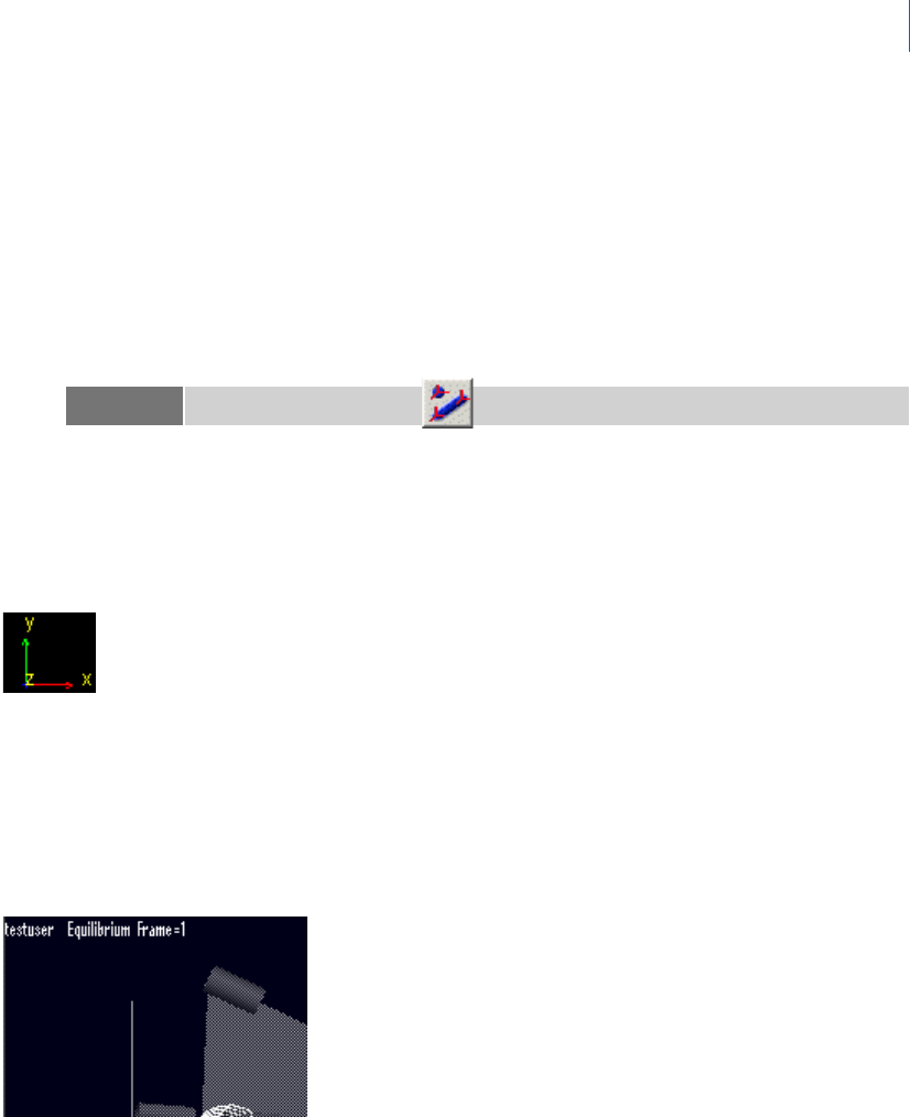
Setting Display of Triad and Title
Triad
You can turn on the display of a triad that displays the orientation of the global coordinate system axes:
It appears in the lower left corner of a
viewport containing an animation. As you move the view of a viewport,
the triad displays the changes to the coordinate system orientation.
Title
You can also display a title for the animation in the upper left corner of the viewport. It displays the name of
the model and the current frame number. During the animation, it displays the time. In addition, you can
set it so it displays the number of frames per second.
To display triad during an animation:
1. From the dashboard, select View.
2. Select Display Triad.
Tip: On the Main toolbar, select .
Adams PostProcessor
Controlling the Animation Display
16
To display title during an animation:
1. From the dashboard, select View.
2. Select Title.
3. To also display the number of frames per second, select FPS Title.
Changing Part Display
You can change the display of individual parts in your animation, including their visibility, color, icon size,
and transparency.
To change the display of parts:
1. Select the part or parts to be changed.
2. In the
Property Editor, set how you want the object displayed. (See Property Editor - Modeling Object.)
Zooming the Display
You can define the area of an animation or plot that you want enlarged and displayed in the current viewport.
You draw a box to define the zoom area.
To define a zoom box:
1. On the View menu, point to Position/Orientation, and then select Zoom Box.
2. Place the cursor where you want the upper right corner of the box and click and hold down the left
mouse button.
3. Drag the mouse diagonally to define the size of the box.
4. Release the mouse button.
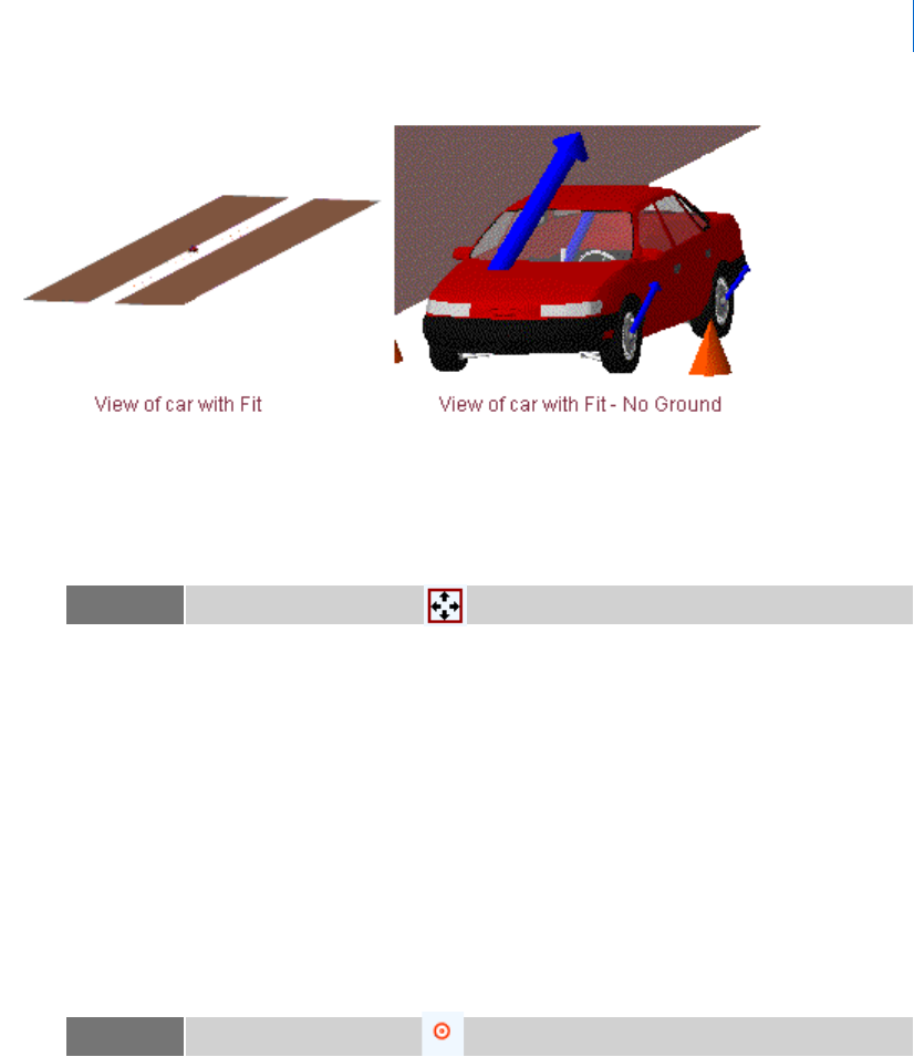
Fitting the Display
You can automatically fit an animation or plot into the current viewport using the Fit and Fit - No Ground
commands. Fit fits the entire model into the window, including the ground part and any geometry attached
to it. Fit - No Ground excludes the ground part and its geometry.
For example, if you have a model of a car that also has a very large piece of geometry on ground representing
a road, and you use Fit to view the entire model, the viewport contains all of the geometry, as shown in the
image on the left in the following figure. It is difficult to observe the car after the fit operation with the ground
included. If you use Fit - No Ground, the viewport is only of the car, as shown in the image on the right.
Tip: On the Main toolbar, select .
17
Animating Results
Controlling the Animation Display
Car and Road with Fit and Fit - No Ground
To fit the entire animation into the viewport, including ground:
On the View menu, point to Position/Orientation, and then select Fit.
To fit the animation, excluding ground, into the viewport:
On the View menu, point to Position/Orientation, and then select Fit - No Ground.
Setting the Center of a Viewport
You can move a particular point in your animation or three-dimensional plot to the center of the current
viewport. You can also reposition the model or plot so that the origin (0,0) of the window is again at the center
of the viewport.
To set a particular point as the center of a viewport:
1. On the View menu, point to Position/Orientation, and then select Center.
2. Click the left mouse button on the point in the model that you want at the center of the window.
To return the origin (0,0) of the viewport to the center of the viewport:
On the View menu, point to Position/Orientation, and then select Origin.
Tip: On the Main toolbar, select .
Tip: On the Main toolbar, select .
Adams PostProcessor
Controlling the Animation Display
18
Setting the View Perspective
By default, Adams PostProcessor displays your animation or three-dimensional plot as though it were drawn
on a flat piece of paper. This is called orthographic projection. You can change the depth of the screen to
perspective projection. Perspective projection causes a vanishing point effect by showing the size of parts
relative to their distance from the viewer. It does not show the true proportions of all parts.
To set the current viewport to perspective, do one of the following:
On the View menu, point to Projection, and then select Perspective.
From the dashboard, select View, and then select Perspective.
To set the perspective in the viewport:
1. On the View menu, point to Position/Orientation, and then select the Translate Z.
2. Place the cursor in the viewport and move the cursor upwards to increase perspective and downwards
to decrease the perspective.
3. To stop setting the perspective, right-click the viewport.
Setting Rendering Mode of Animations
Adams PostProcessor provides four rendering modes in which you can display an animation in a viewport, as
listed in the table below.
Rendering Modes
To select a rendering mode:
1. Click the viewport whose rendering mode you want to change.
2. On the View menu, point to Render Mode, and then select a rendering mode.
Tip: From the Main toolbar, right-click , and then select .
The mode: Does the following:
Wireframe Shows only the edges of objects so that you can see through the objects.
Shaded (flat) Shaded, but polygon edges are visible.
Smooth shaded Shaded, with polygon edges not visible.
Hidden-line removal Shows only the edges of object. It does not show edges, or portions of edges, that
are obscured by other geometry.
Tip: To toggle between shaded and wireframe, on the Main toolbar, select .
19
Animating Results
Controlling the Animation Display
Specifying the Camera Perspective
You can change your viewing or camera perspective. For example, you can change the perspective to always
look at a particular part as it moves or to always look from a particular vantage point, such as one that moves
with a part. Setting different camera perspectives is particularly helpful when parts undergo large motions
and move off your screen during an animation, such as with vehicle simulations.
A good example of setting the camera perspective is when you simulate a vehicle driving through a slalom
course on a test track. By default, you view the simulation as a bystander alongside of the road whose gaze is
fixed in one direction. As the vehicle moves forward, it quickly moves out of your field of view. You can,
however, set the camera perspective to mimic the movement of your head as it moves to follow the vehicle.
Furthermore, rather than observe the vehicle as a bystander alongside a road, you can also set the camera
perspective to mimic what the driver sees as he or she looks out the front windshield of the vehicle.
To set the camera perspective:
1. From the Dashboard, select Camera.
2. Set the options as explained in the table below.
3. Select Lock Rotations to follow the rotations of the followed object.
4.
Play the animation.
Camera Perspective Options
Setting Lighting
Adams PostProcessor has many lighting options to help you enhance the quality and realism of your
animations. The options allow you to set:
Overall intensity of the light (much like setting a dimmer switch in your home).
Note: If you are using the Native Open GL graphics driver, which is the default, only two
modes have an effect: wireframe and smooth shaded. For more information on
selecting graphics drivers, see
Running and Configuring Adams.
To set the camera perspective
to:
In the Follow Object text box: Mount Camera At text box:
Follow a moving point Enter the marker that you want to
follow during the animation.
Do not enter a marker. Leave it
empty.
Look from a movable point
towards a stationary point
Enter a marker on a non-moving
part or ground.
Enter a marker on a moving part.
Look from one movable point to
another
Enter the marker that you want to
follow during the animation.
Enter the marker that you want to
remain in the center of the screen
during the animation.
Adams PostProcessor
Controlling the Animation Display
20
Background, ambient light to control the diffusion of light sources to affect the amount of lighting
on edges.
Reflections off of parts. (Note that this is computationally expensive and can slow down your
animations.)
Focused lighting that comes from different directions, and define the angle of that lighting (how far
it is from the center line). You can think of this as swinging a light boom across your model.
Illumination of only one side of the geometry to speed up your animations.
To access the lighting options:
From the dashboard, select View.
To set up overall light intensity, ambient lighting, and reflections:
1. Use the Light Intensity slider to set how bright the overall light is.
2. Use the Ambient Light slider to set the ambient light.
3. Toggle Light Reflections to set up reflections off of parts.
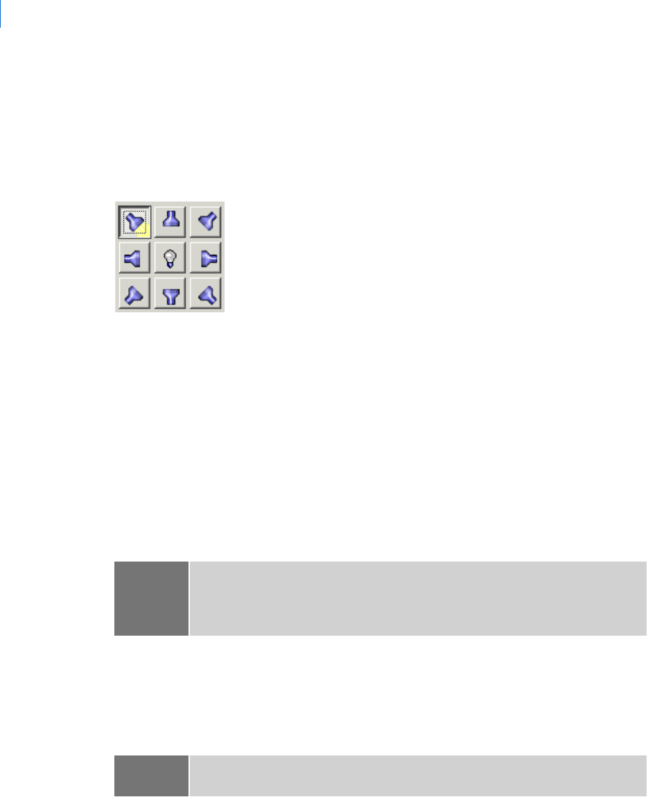
To set up focused lighting:
1. Use the light buttons on the right side of the dashboard to turn on different focused light sources.
2. Use the Light Angle slider to set how far from the center line the light source is.
To set up one-side lighting:
Clear the selection of Two-Sided Lighting.
Note: The number of light sources you can select depends on the graphics driver and system
you are using. If you selected OpenGL, the number of light sources depends on your
graphics card. For more information on selecting graphics drivers, see
Running and
Configuring Adams
.
Note: To achieve the fastest animations, set the lighting options to either: No reflections;
One-sided; or One light source.

21
Animating Results
Animating Flexible Bodies and Adams Durability Results
Animating Flexible Bodies and Adams Durability Results
Learn more about animating flexible bodies and Adams Durability results:
Caching of Flexible Bodies
Animating Only the Flexible Body
Setting Animation Display Options for Flexible Bodies
Animating Deformations, Modal Forces, and Stress/Strain
Caching of Flexible Bodies
When you select to animate a model containing flexible bodies, Adams PostProcessor creates a flexible body
cache file (.fcf) that contains the animation data for the flexible bodies. By creating a cache file, Adams
PostProcessor reduces the memory usage required when animating models with flexible bodies, while
maintaining peak animation performance.
You can change the type of caching and set other preferences as explained in
PPT Preferences - Animation.
Animating Only the Flexible or Stress Body
When animating flexible or rigid stress bodies, you can also select to only display the flexible or stress body
and no other parts. The selected body appears without any of the translational or rotational information from
the analysis. This allows you to focus in on contour plot information, as well as the hot spot information for
both flexible and stress bodies. Also, with flexible bodies, this allows you to focus on a particular body and
watch its deformations within the animation or analyze any color information.
To display only a flexible body:
1. From the Dashboard, select Animation.
2. Right-click the Component text box, and point to Flexible Body or Rigid Stress Body, and then use
the menus to select a body to display.
3.
Play the animation.
Setting Animation Display Options for Flexible Bodies
You can set various animation options for flexible bodies, including scaling the deformation of a flexible body
while it is being animated, setting the rendering of the flexible body, and setting the type of plot to display.
Learn more about flexible body plots.
Also learn about:
Setting the defaults for animations of flexible body deformations and display of vector plots with PPT
Preferences - Animation
Tuning the performance of flexible bodies
Setting general display options for objects
Adams PostProcessor
Animating Flexible Bodies and Adams Durability Results
22
To set the animation options:
1. In the treeview, select the flexible body on which you want to set animation options.
2. In the
Property Editor, select the tab Flex Props.
3. Set the properties for the animation. (Learn more about the property editor for changing animation
display with
Property Editor - Flexible Body dialog box help.)
Animating Deformations, Modal Forces, and Stress/Strain
You can select to animate the deformations, modal forces (MFORCEs), or the stresses and strain acting on
the flexible body as
Contour plots or Vector plots. You can also animate both types of plots on the same flexible
body.
Learn more about color contour and vector plots:
About the Data the Different Types of Plots Display
Displaying Plots
Specifying a Deformation Datum Node
Modifying Contour Legends
About the Data the Different Types of Plots Display
Depending on the Adams product you use to create and simulate your model, you display different types of
data as contour or vector plots: deformations, stress/strain, or modal forces:
Data and Type of Plot
You can view: As: Using data from:
Deformations Contour plots Adams Flex - When you analyze flexible bodies using Adams Flex,
you can contour deformations using Adams View or Adams
PostProcessor.
Stress/Strain Contour plots Adams Durability - When you obtain stress and strain results using
Adams Durability, you can use Adams PostProcessor to show the
stress and strain on a body as contour plots. The stress or strain can
be contoured on rigid or flexible bodies. For more on obtaining
stress and strains, see the
Adams Durability online help.
Modal forces Contour and
vector plots
Adams View and Adams Flex - You can contour MFORCEs in
Adams PostProcessor as both contour and vector plots. You can only
view force or torque vectors as vector plots.
For more information on MFORCES, see
Modeling Distributed Loads
and Predeformed Flexible Bodies
.
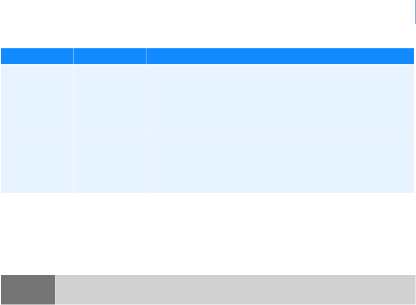
23
Animating Results
Animating Flexible Bodies and Adams Durability Results
Displaying Plots
To display color contour or vector plots, you must first specify the flexible body on which you want to display
the plots and which types of plots to display, and then turn on the plots.
To turn on contour and vector plots for individual flexible bodies:
1. In the Treeview, select the flexible body on which you want to display plots.
2. In the
Property Editor, set Plot Type to the appropriate type of plot (Contour, Vector, or Both).
To turn off the display of contour and vector plot for individual flexible bodies:
1. In the treeview, select the flexible body which is set to display plots.
2. In the property editor, set Plot Type to None.
To display a contour plot in a particular view:
1. From the dashboard, select Contour Plots.
2. From Plot Type, select a type of contour plot.
To display a vector plot:
1. From the dashboard, select Vector.
2. From Plot Type, select a plot.
Kinetic/Strain Contour plots Adams Vibration – When you compute kinetic or strain energy
distribution results using Adams Vibration, you can use Adams
PostProcessor to display these as contours on flexible bodies in the
model. These contours can be displayed during mode shape or
vibration animation
Strain SS Contour plots Adams Vibration – When you compute frequency response for
models with flexible bodies, you use Adams PostProcessor to display
the strain energy contours during a mode shape or vibration
animation. This only applies if the .mnf files for the flexible bodies
contain stress-strain modes.
You can view: As: Using data from:
Note: You can also set the flexible body contour and vector plotting in Flexible Body Modify dialog
box
. See the Adams Flex online help.

Adams PostProcessor
Animating Flexible Bodies and Adams Durability Results
24
Specifying a Deformation Datum Node
You can set the datum node for which you want deformations to be relative to. Adams PostProcessor considers
the deformation to be relative to the origin of the flexible body (its local body reference frame (LBRF) or
coordinate system) by default. For example, if you were modeling a cantilever beam in Adams Flex, you could
specify that deformations should be relative to the clamped end.
To specify a datum node:
1. In the treeview, select the flexible body on which you want to display plots.
2. In the Property editor, in the Datum Node text box, enter the number of the desired node.
3. Select OK.
Modifying Contour Legends
For each viewport, you can change the way contour plots display colors and values. Please note that this allows
you to display different viewports at the same time but with different color values, which can be confusing
because a color value in one viewport may not be the same as in another.
To turn off the legend:
Clear the selection of Display Legend.
To modify the legend:
1. From Legend Placement, select where you'd like the legend to appear.
2. In the Legend Title text box, change the text of the legend title.
3. In the Colors text box, enter the number of colors to be displayed in the plot. There can be no more
than 255.
4. In the Minimum and Maximum text boxes, enter the minimum and maximum values for the plot.
5. In the Decimal Places text box, enter the number of decimal places to which the numbers in the axes
should be displayed.
6. In the Scientific Range text boxes, enter the exponential form for scientific notation.
To reset the legend values based on the flexible bodies in the active view:
Select Reset Limits.
Note: To select a node from the screen, right-click the Datum Node text box, and then select
Pick Flexbody Node. Select the node from the screen. The node number appears in
the Datum Node text box.

25
Animating Results
Animating Flexible Bodies and Adams Durability Results
Tuning the Performance of Flexible Body Animations
You can use the Animation Performance Tuning guide to help you improve the performance of the animation
of flexible bodies. It steps you through all the options available in Adams PostProcessor. These same options
are located throughout the Adams PostProcessor interface. It also provides tips on optimizing modal neutral
files (MNFs) for best animation performance.
To run the Animation Performance Tuning guide:
1. From the Tools menu, select Animation Performance Tuning.
2. Follow the prompts and enter the values to improve the animation performance of flexible bodies.

Adams PostProcessor
Animating Flexible Bodies and Adams Durability Results
26

1
Building Plots
Plots Basics
Building Plots
You can plot the results of any Simulation to interpret the performance of your design. You can plot the results
for any
Measures or Requests that you defined, as well as results that Adams automatically generates, including
clearance studies. You can even plot test data that you imported into Adams PostProcessor and perform post-
processing on the plot curves.
You use the
Dashboard in plotting mode to select simulation results to plot. After you select simulation results
to plot, you can format the resulting plots, including adding the necessary axes, labels identifying the units
of measurement, title for the plot, legends describing the data in the plots, and more. You can also build three-
dimensional plots using Adams Vibration. The three-dimensional plots display a collection of curves.
Learn
more about generating data for three-dimensional plots in the Adams Vibration online help
.
Plots Basics
About Curves on Plots
Curves on plots are made up of data points. Each data point represents data that the Adams product created
at an output step during a simulation, test data that you've imported, or data from Adams Solver files (
Request
file
or Results file). For results from a simulation, you specify the number of output steps when you perform a
simulation, and, thus, you set the number of data points in a curve. For information on setting output steps,
refer to the Adams product documentation you used to create the simulation results.
After you created curves, you can perform post-processing operations on curves, such as filter the data
through signal processing or mathematical calculations. You can also manually change the values and write
expressions that define the values in curves. For more information on post-processing on curves, see
Performing
Calculations on Curves
and Manipulating Curve Data.
Types of Simulation Results You Can Plot
Adams provides you with several different types of results that you can plot. Some of the results you must
request and some Adams products generate automatically.
Objects - Characteristics of objects in your model, such as the position of the center of mass of a part
for the x component. They correspond directly to object measures. To view objects, you must run
Adams PostProcessor with Adams View or import a
Adams View command file (.cmd).
Measures - Characteristics of quantifiable objects in your model, such as the force applied on a
spring-damper or the relationship between objects. You can create measures directly in an Adams
product or import test data as measures. To view measures, you must run Adams PostProcessor with
Adams View or import a model and a
Results file (.res).
Learn:
• About Viewing test data
• About Measures

Adams PostProcessor
Plots Basics
2
Results - A basic set of state variable data that Adams calculates during a simulation. Adams outputs
the data at each simulation output step. A component of a result set is usually a time series of a
particular quantity (for example, the x displacement of a part or the y torque on a joint).
Requests - Data that you have requested that Adams Solver output. You can ask for any type of
displacement, velocity, acceleration, force or user defined filter information that you want to
investigate.
• If the "Define Using Type and Markers" method is used, the requests appear under the
displacement, velocity, acceleration, or force filters.
• If the "Define Using Function Expression" method is used, the requests appear under the "user
defined" filter.
• If the "Request Name" and "Result Set Name" are exactly the same, the request appears under
the Subsystem heading, but if they are different, then the request appears at the top level.
• If component names and component units are given, but the results name is not specified, then
the request will appear in the “Result Sets” list.
System modes - You can view scatter plots of the eigenvalues from linear simulations.
Clearance studies - You can view the minimum distances between objects in your animation. Learn
about
Performing Clearance Studies.
For Adams Vibration, you can also plot the following:
Frequency Response - The magnitude and phase response produced by a given input channel, at a
given omega, for a given output channel.
Transfer Function - Transfer function is a basic property of a model, and is computed as the
magnitude and phase response at a given output channel for a given input channel with a unit swept
sine vibration actuator.
PSD - Power spectral density of output channels for given input PSDs.
Modal Coordinates - Modal coordinates are states in the frequency domain solution associated with
a specific mode. Modes most active in a frequency response can be identified from the modal
coordinates.
Modal Participation - The absolute contribution of model modes to the transfer function for the
model.
Learn about
Plotting Adams Vibration Output in Adams PostProcessor.
See the
Adams View Object Characteristics You Can Plot for more information.
About the Dashboard in Plotting Mode
When you are in plotting mode, the Dashboard lets you select the data that you want to plot. The dashboard
in plotting mode is shown below.
Learn more about the
Plotting Dashboard.
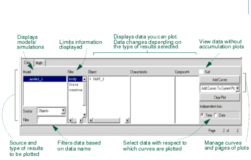
3
Building Plots
Plots Basics
The list on the left side of the Plot Builder contains the simulation results that are available for plotting. These
include objects, measures, requests, result sets, and system modes. The list contains the models or results you
have loaded and is set to view object characteristics. If you have three different models loaded, the list of
models would look like the following:
.model_1
.model_2
.model_3
If you are viewing requests, measures, or results, the list contains the names of all the simulations you've
imported into Adams PostProcessor. For example, if you have three different models and two simulations on
model_3, then the list looks like the following:
.model_1.Last_Run
.model_2.Last_Run
.model_3.Last_Run
.model_3.Run_001
Because you see all the simulation results at once, it is easy for you to plot results between simulation runs
and even between simulations from separate models (for example, plot body acceleration from one model
against another model).
Plotting Objects
You can plot characteristics of objects in your model. You do not need to create object measures to plot object
characteristics. You can select to display more than one object characteristic at a time.
To plot objects, you must run Adams PostProcessor with Adams View or import model and results.

Adams PostProcessor
Plots Basics
4
To create a plot of object data:
1. From the Dashboard, set Source to Objects.
The dashboard changes to show the results available for plotting.
2. Select a model whose object characteristics you want to plot.
3. From the Object list, select the object whose characteristics you want to plot. The Object list contains
a list of all the objects in your model that are of the type specified in the Filter list.
Learn about Filtering
Lists of Data to be Plotted
.
4. From the Characteristic list, select the characteristic of the selected object that you want to plot.
5. From the Component list, select one or more components of the characteristic that you want to plot.
6. Select Add Curves to add the data curve to the current plot.
Plotting Measures
To create a plot of measure data:
1. From the Dashboard, set Source to Measures.
The dashboard changes to show the measures available for plotting.
2. From the Simulation list, select a simulation. The list contains all the potential sources of data for
creation of plots. As you add additional simulation results, these appear in the Simulation list.
3. Select the measure or measures that you want to plot. Learn about
Selecting and Deselecting Objects in
Adams Postprocessor.
4. Select Add Curves to add the data curve to the current page.
Plotting Requests and Result Sets
Adams PostProcessor supports both plotting of Request file (.req) and Result set component (.res).
To create a plot of a result or request component:
1. From the Dashboard, set Source to:
• Requests - Plot request components.
• Result Sets - Plot any result components from a simulation.
The dashboard changes to show the results available for plotting.
2. From the Simulation list, select a simulation. The list contains all the potential sources of data for
creation of plots. Any new simulations that you add, appear in the Simulation list.
3. From the Result Set or Request list, select a result or request.
4. From the Component list, select components to plot. Learn about
Selecting and Deselecting Objects in
Adams Postprocessor.
5. Select Add Curves to add the data curve to the current plot.

5
Building Plots
Plots Basics
Plotting System Modes
You can create a scatter plot of eigenvalues from a Linear simulation. You plot the real eigenvalues against the
imaginary eigenvalues. In addition, you can plot the eigenvalues with a table of eigenvalues. See
Picture of
Plotting System Modes
.
Learn about setting the color and symbols of the scatter plot with
Property Editor - Scatter dialog box help.
To plot a scatter plot of eigenvalues:
1. From the Dashboard, set Source to System Modes.
2. From the Eigen list, select a set of eigenvalues.
3. Select Add Curves to add the scatters to the current plot.
To plot a scatter plot with an eigen table:
1. From the dashboard, set Source to System Modes.
2. From the Plot menu, select Create Scatter Plot with Eigen Table.
3. If you have more than one one eigen in the database, select the eigen of interest.
The scatter plot appears.
Viewing Test Data
You can easily import test data by reading in an ACSII file using the Import command on the File menu.
Learn about importing test data.
Adams PostProcessor imports test data from a column-based file and stores the data as
Measures. Once Adams
PostProcessor has imported the test data as a measure, you can plot, display, or modify it as you would with
any other measure.
Learn about plotting measures.
Quickly Reviewing the Results of Simulations
You can quickly scan the results of your simulation without having to create a large number of plot pages.
This is called surfing.
Note: In some cases when requests are present in a model there will be an additional analysis
listed in the plotting dashboard named "REQSAVE_COMPATIBILITY". See "
About the
"REQSAVE_COMPATIBILITY" analysis
" for details.
Note: If you're plotting Adams Vibration data, you can also create the plot by selecting
Vibration -> Review -> Create Scatter Plot with Eigen Table.

Adams PostProcessor
Plots Basics
6
To surf results:
1. From the right side of the Dashboard, select Surf.
2. Select the simulation results you want to plot.
Adams PostProcessor automatically clears the current plot and displays the simulation results after
you make each selection.
3. Continue selecting simulation results to plot.
Adding Curves to Plots
You can add as many curves as you'd like to a plot. You can also choose to create a new plot each time you
add a curve or create a different plot for each
object, request, or result you select to plot. For example, Adams
PostProcessor lets you automatically plot the velocity, acceleration, and placement of a single object on a plot.
When you plot data about a different object, you can set Adams PostProcessor to automatically create a new
plot for the data.
If you choose to add curves to the currently selected plot, Adams PostProcessor assigns each new curve a
different color and line style so you can differentiate the curves from one another. For example, the first curve
you create is red, the next blue, and the third magenta. You can change the automatic assignment of properties
to a single color, style, and symbol that you define.
Learn about setting curve properties.
Adams PostProcessor creates a dependent (vertical) axis for each unit type. For example, if you plot
displacement and velocity on the same plot, then Adams PostProcessor automatically displays two dependent
axes (one for displacement and one for velocity).
To add curves:
1. Select the results to plot.
2. From the pull-down menu located below the Add Curves button on the
Dashboard, select how you'd
like Adams PostProcessor to add the curves. You can select:
• Add Curves to Current Plot - Adds the curve to the currently selected plot.
• One Curve Per Plot - Creates a new plot on a new page for the curve.
• One Plot Per Object, Request, or Result - Creates a new plot for the curves containing data about
a particular object, request, or result. (Not available for measures.)
3. Select Add Curves.
Using an Independent Axis Other Than Time
The default data used for the independent axis of a plot is simulation time. You can use other data than
simulation time.
Note: The independent axis, by default, is along the x-axis. To change its position, see Setting Up
Plot Parameters
.

7
Building Plots
Plots Basics
To select data other than time:
1. From the right side of the dashboard in the Independent Axis area, select Data.
The Independent Axis Browser appears.
2. Select the desired data, and then select OK.
Filtering Lists of Data to be Plotted
The Filter list in the dashboard lets you select a subset of all the possible data to be displayed. This is
convenient for large models where the object list could be very long and difficult to read. In addition, you
can filter lists of data based on their name. For example, you can specify that Adams PostProcessor only
display objects that start with PART_.
To filter the data to be displayed:
From the Filter list, select the type of data that you want to display. The objects available to display
depend on the type of results you selected.
For information on selecting more than one object in the Plot Builder, see
Selecting Objects in Adams
PostProcessor
.
To filter on the name of data:
Below Source, in the Filter text box, enter the name of the data that you want to display. Type any
wildcards that you want included. For more on wildcards, see
Using Wildcards.
Updating Plot Data
If you are iteratively changing your model and reviewing results, you will find that the Replace Simulations
command saves you lots of time. You can update the data in the plots with that stored in simulation result
files, without recreating the plots. You can also add data from other simulations to your existing plots.
When you update your plots, Adams PostProcessor looks for simulation results in the original simulation
Results file (for example, a Request file) from which you imported the current data. If the time and date stamp
on the original file is more recent than the time and date stamp on the plot, Adams PostProcessor reloads the
plot with the updated data.
If you use the Add Simulation option, a new legend, called the simulation legend, appears on the left side of
the plot. The simulation legend identifies the source of the data grouped by color or line style. The original
legend, called the curve legend, continues to show information about the original curves.
To update your plot data:
1. On the File menu, select Replace Simulations.
Tip: From the Main toobar, select .

Adams PostProcessor
Plots Basics
8
The Add/Replace Simulations dialog box appears.
2. In the upper left corner of the dialog box, select either of the following option buttons:
• Add Simulation to add new curves.
• Replace Simulation to update the curves already on the plot.
3. In the Runs text boxes, enter the name of the simulation containing the simulation results to be
replaced. By default, the results of the last simulation (Last_run) replaces any simulation results that
the curves use.
4. Set the color, line style, and weight for the new or existing (old) curves. If you select No Change,
Adams PostProcessor uses the current color of the curve representing the data to be added or replaced.
Select Auto to allow Adams PostProcessor to automatically assign colors to the curves.
5. In the Update Pages area, select the pages containing the plots that you want to update.
6. Select OK.
Clearing Plot Data
You can quickly remove all curves on the current plot.
To clear plot data:
On the right side of the dashboard, select Clear Plot.
Displaying Plot Statistics About Curves
You can display statistics about curves, including:
Coordinates of individual data points.
Minimum, maximum, and average values of visible data points.
Average slope of the curve at individual data points.
Root mean square (RMS) calculation of dependent values over the entire curve.
Number of points of the curve used in statistics computations.
You can also find the distance between two data points and the magnitude of the cursor excursion.
Adams PostProcessor displays plot statistics either using the numeric format of the curve's axis or the numeric
format of the table column (if the plot is displayed as a table). The curve format takes precedence if it is set.
When you choose to display statistics, Adams PostProcessor displays a Statistics toolbar as shown below.
Note: Adams PostProcessor uses only the portion of the curve between the horizontal axis limits
when it performs the minimum, maximum, average, and RMS calculations, as well as when
it determines the number of points used in a calculation. To inspect statistics on a subset of
the curve, zoom in on a subset of the curve.
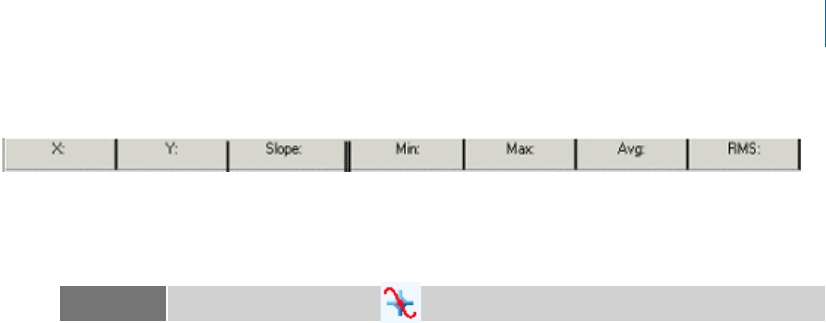
9
Building Plots
Plots Basics
Statistics Toolbar
To toggle on and off the display of the Statistics toolbar:
On the View menu, point to Toolbars, and then select the Statistics Toolbar.
The Statistics toolbar appears at the top of the window below any toolbars that you've already
displayed. A vertical line appears at the currently selected data point.
To display statistics about different data points on a curve:
Select a different data point. To select a data point, you can either:
• Use the left and right arrow keys to move from data point to data point along a curve.
• Use the mouse to move the cursor to another data point.
• Use the up and down arrow keys to move between curves.
To display the local maximum data points:
Hold down the Shift key and use the left and right arrow keys to move from one local maximum
data point to another.
To display the local minimum data points:
Hold down the Ctrl key and use the left and right arrow keys to move from one local minimum data
point to another.
To determine the distance between two data points:
1. Select the first data point and press and hold down the left mouse button.
2. Drag the cursor to the next data point.
Adams PostProcessor displays the distance between the two data points in the Statistics tool bar. It
places a D in front of the coordinate values. Adams PostProcessor also displays a MAG text box,
which displays the magnitude of the cursor displacement. The magnitude is the square root of the
sum of the squares of the two coordinate values.
3. Drag the cursor to another data point or release the mouse button.
Tip: On the Main toobar, select .

Adams PostProcessor
Plots Basics
10
Listing of Plot Parameters
The parameters you can set for an entire plot are listed below:
Title and subtitle - Lines of text that describe the plot.
Analysis name and date - Automatically display the name of the analysis from which the plot data
was generated, and the date on which the analysis was run.
Legend text - There are two types of legends on a plot:
• Curve legend - Text that describes the data that each curve on the plot represents. Adams
PostProcessor displays the legend with a short line segment illustrating the color and line style of
the curve.
• Simulation legend - If you add simulation data as explained in Updating Plot Data, Adams
PostProcessor creates a second legend, called the simulation legend.
Dependent axis - Set the orientation (vertical or horizontal) of the dependent axis. Note that you
can only change the orientation if there are no curves on the plot.
Grid - A collection of horizontal and vertical lines that serve as visual guides for inspecting curves.
You can have primary and secondary grid lines. Primary grid lines appear at all major unit sections.
Secondary grid lines appear at specified intervals between the primary grid lines. If you turn off the
primary grid lines, Adams PostProcessor also turns off the secondary grid lines.
Borders and plot placement - The ruling lines around the plot and the margins (white space) that
appear on the left and bottom of the screen surrounding the plot.
Notes: If you have turned on plot statistics, you can quickly create a spec line at the current location
of the plot tracking cursor using the keyboard shortcuts:
s or S create vertical speclines.
h or H create horizontal spec lines.
Learn about adding spec lines.
Note: For information on setting Adams PostProcessor so it automatically displays titles, see
PPT Preferences - Plot. For information on modifying the appearance of the text in the
titles, see
Adding Notes and Modifying Text.
Note: For information on modifying the appearance of the text in the legends, see Modifying
Legend Properties
.

11
Building Plots
Controlling the Display of Two-Dimensional Plots
Controlling the Display of Two-Dimensional Plots
For two-dimensional plots, you can control the following:
Zooming in on a Plot
To Pan Within a Plot
To Copy to Clipboard
Fitting a Curve to a Plot
Setting Up 2D Plot Parameters
• Modifying Titles and Axis Placement
• Modifying Plot Borders
• Modifying Primary and Secondary Grid
Zooming In on a Plot
You can define the area of a plot that you want enlarged and displayed in the current window. You draw a
box to define the zoom area.
To define a zoom box:
1. On the View menu, select Zoom Plot.
2. Place the cursor where you want the upper right corner of the box and click and hold down the left
mouse button.
3. Drag the mouse diagonally to define the size of the box.
4. Release the mouse button.
Note: Adams PostProcessor automatically sizes a plot to fit in the viewport. The axis limits, notes,
and axis values do not change but the aspect ratio of the plot border changes based on the
aspect ratio of the viewport.
Note: You can also zoom in on an area of a plot by setting the minimum and maximum values to
be displayed on the plot axes.
Learn about modifying axis attributes.
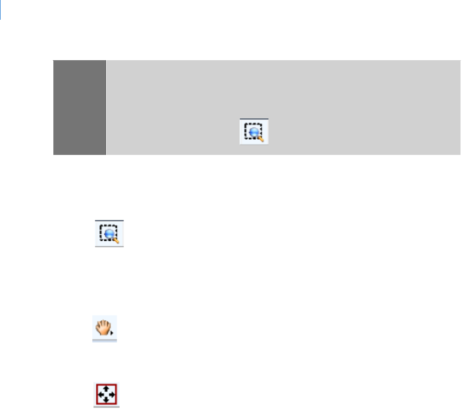
Adams PostProcessor
Controlling the Display of Two-Dimensional Plots
12
To Pan Within a Plot
a. Zoom in on a section of the plot via the area-zoom button (or via the newly-added keyboard
shortcut “w”)
b. Once the plot is zoomed, use the left/right and up/down arrow keys on the keyboard to pan
within the plot
c. Alternatively, do a dynamic pan using the new pan button (or via the keyboard shortcut “p”).
Press the “Esc” key to exit pan mode.
d. Plot can be re-fit to its entire extent by clicking the fit button (or via the newly-added keyboard
shortcut “f”)
To Copy to Clipboard
a. To copy the contents of the entire page, right-click the page from the treeview and select “Copy
- To Clipboard”. Both the animation pane and the plot pane can now be pasted as a single image
into Word
®
or PowerPoint
®
(for example) by those applications’ “Paste” buttons or via Ctrl+V.
Tip: Either:
Click and hold down the middle mouse button when the cursor is in the window and
drag the mouse to define a zoom box.
On the Main toolbar, select .
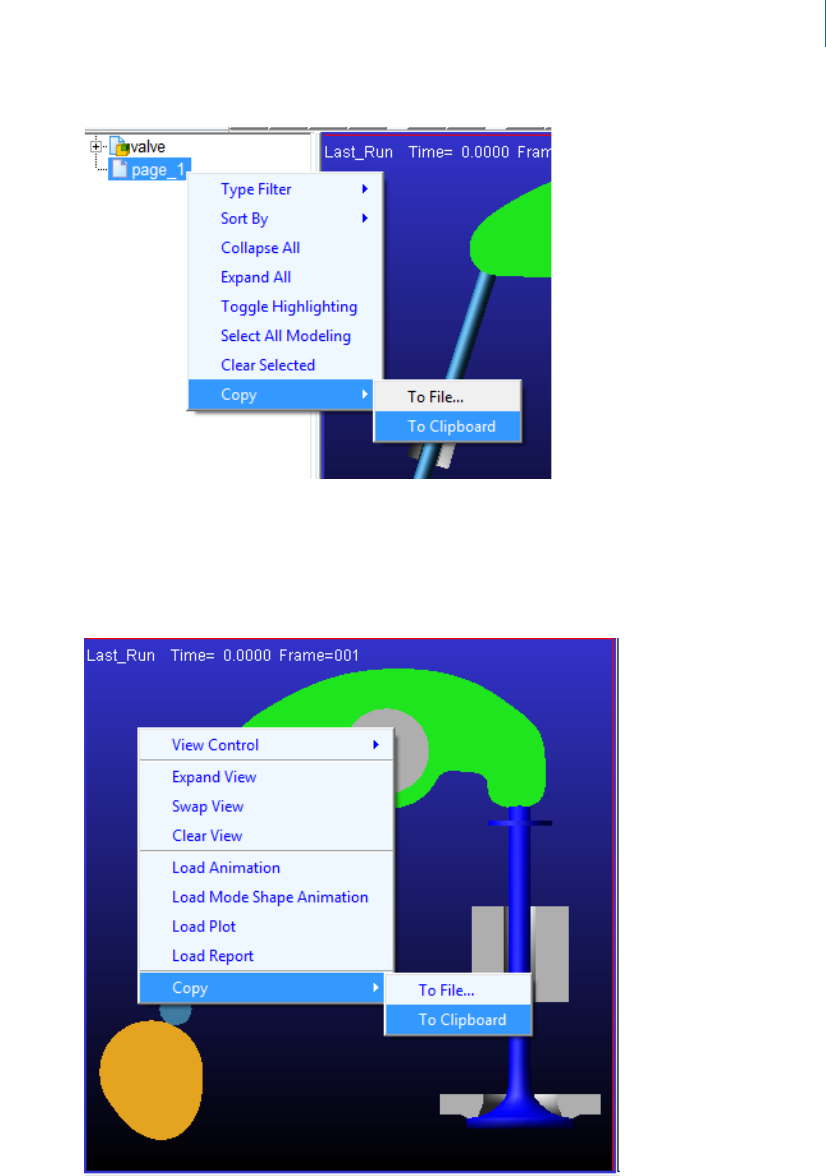
13
Building Plots
Controlling the Display of Two-Dimensional Plots
b. To copy the contents of an individual pane, select that pane by clicking in it and then right-click
in empty space on the given pane and select “Copy - To Clipboard” (or use keyboard shortcut
Ctrl+C). The content of that particular pane can now be pasted as a single image into Word
®
or
PowerPoint
®
(for example) by those applications’ “Paste” buttons or via Ctrl+V.

Adams PostProcessor
Controlling the Display of Two-Dimensional Plots
14
Fitting a Curve to a Two-Dimensional Plot
You can scale all the curves on a plot so that they fit entirely within a viewport.
To fit curves to a plot:
From the View menu, select Fit Plot.
Setting Up Two-Dimensional Plot Parameters
The following figure shows some of the plot parameters that you can set for a 2D plot. See Listing of Plot
Parameters
.
Learn more about them and how to set them up:
Modifying Titles and Axis Placement
Modifying Plot Borders
Modifying Primary and Secondary Grid
Tip: Either:
Click and hold down the middle mouse button when the cursor is in the window and
drag the mouse to define a zoom box.
On the Main toolbar, select .
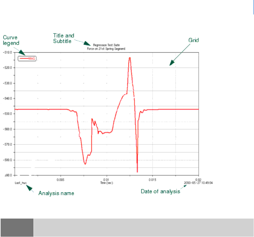
15
Building Plots
Controlling the Display of Two-Dimensional Plots
Plot Parameters
Modifying Titles and Axis Placement
To set plot parameters for title, subtitle, and axis placement:
1. Select a plot.
2. In the
Property Editor, select General.
3. Set the title and subtitle:
• To have Adams PostProcessor automatically generate titles and subtitles, select Auto Title or Auto
Subtitle.
• To create your own titles and subtitles, clear the selection of Auto Title or Auto Subtitle, and in
the Title and Subtitle boxes, enter the text for the title and subtitle. The title and subtitle can only
be a single line of text.
Learn how to modify the text and have multi-line titles.
4. To have the analysis name and the date on which the analysis was generated appear on the plot, select
Analysis and Date Stamp.
Note: You can also set up pages so that they have headers and footers. For more information, see
Displaying Headers and Footers on Pages.
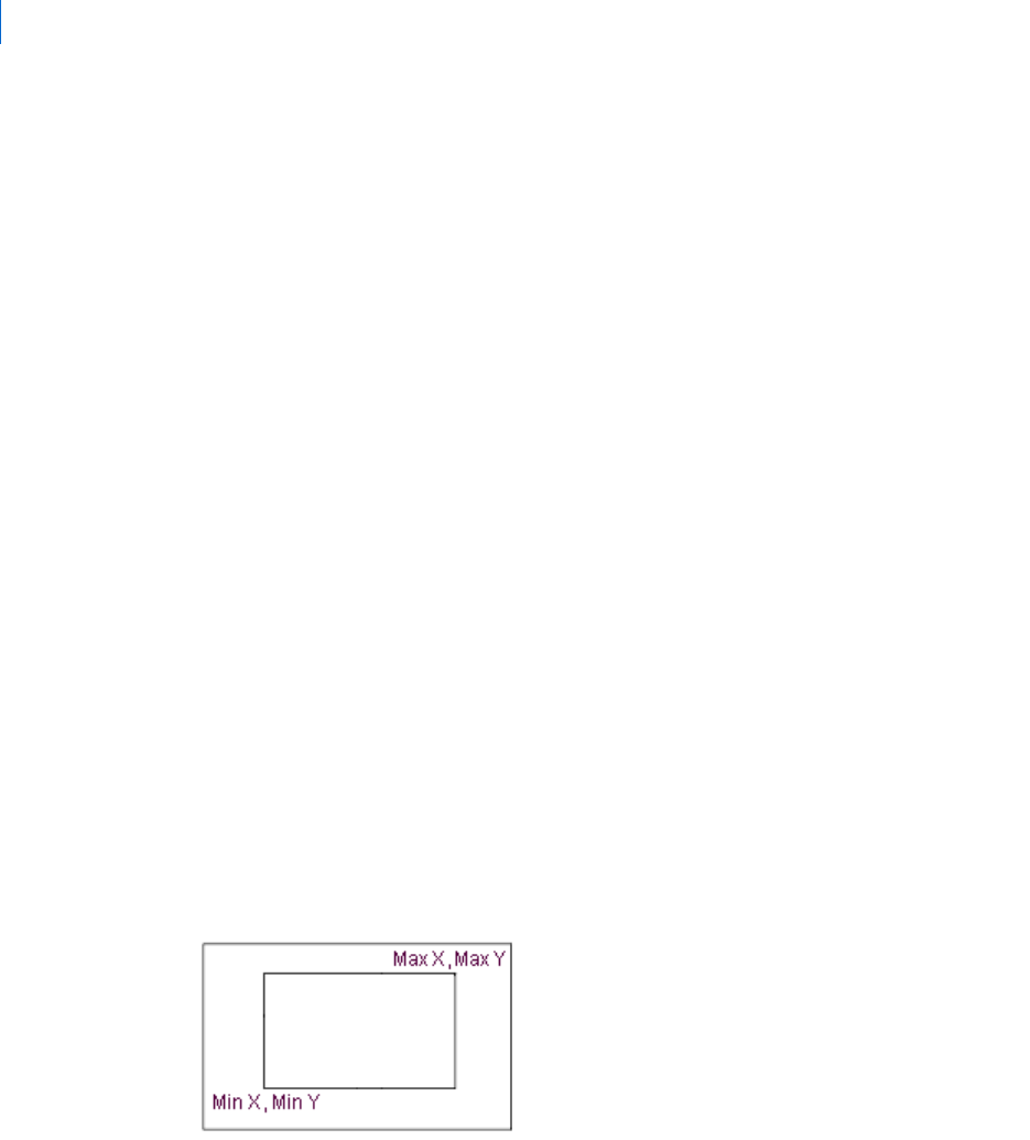
Adams PostProcessor
Controlling the Display of Two-Dimensional Plots
16
5. To add legend text, select Legend. Learn about modifying legend properties.
6. To create a line at the position 0,0, select Zero Line.
7. Set where you want the dependent axis of data to appear by selecting either Horizontal (along the x-
axis) or Vertical (along the y-axis). Note that you can only change the orientation if there are no
curves on the plot.
Modifying Plot Borders
To modify a plot border:
1. Select a plot.
2. In the
Property Editor, select Border.
3. Set Color to the color for the border.
4. Select the type of line style and weight for the border. The weight values range from 1 to 5 screen
pixels.
5. Set up the placement of the plot:
• To center the plot in the viewport and keep it centered even when you make modifications to its
layout, select Auto Fit Border.
• To set your own margins for the plot, clear the selection of Auto Fit Border and enter the
minimum and maximum values for the margin in the x and y directions in pixels. See the figure
below for assistance.
Min X - Sets the space from the left edge of the window to the left edge of the plot.
Max X - Sets the width of the plot. It includes the left margin that Min X defines.
Min Y - Sets the size of the space from the bottom edge of the window to the bottom edge of the
plot.
Max Y - Sets the height of the plot including the bottom margin that Min Y defines.
Minimum and Maximum Values for Borders

17
Building Plots
Controlling the Display of Three-Dimensional Plots
Modifying Primary and Secondary Grids
Adams PostProcessor displays grids on a plot to provide visual guides for inspecting curves. You can have
primary and secondary grid lines. Primary grid lines appear at all major unit sections. Secondary grid lines
appear at specified intervals between the primary grid lines. If you turn off the primary grid lines, Adams
PostProcessor also turns off the secondary grid lines.
To modify the properties for the primary or secondary grid:
1. Select a plot.
2. In the
Property Editor, select Grid or 2nd Grid.
3. To turn off the display of the grid, clear the selection of Visible.
4. From the pull-down menu, set the number of lines by either selecting:
• Line Count and entering the number of lines in the grid.
• Increment and entering the amount of space between each grid line in the x and y directions.
Enter the values in length units.
5. Select a line style, weight, and color for the primary grid. The weight values range from 1 to 5 screen
pixels.
Controlling the Display of Three-Dimensional Plots
(Available for Adams Vibration data only)
For three-dimensional plots, you can control the following:
Zooming in on a Three-Dimensional Plot
Fitting a Curve to a Three-Dimensional Plot
Setting the Center of a Three-Dimensional Plot in a Viewport
Setting the View
Rotating and Translating the View
Specifying Rendering Mode
Setting Up Three-Dimensional Plot Parameters
Zooming In on a Three-Dimensional Plot
You can define the area of a plot that you want enlarged and displayed in the current window. You draw a
box to define the zoom area.
Note: You can also zoom in on an area of a plot by setting the minimum and maximum values to
be displayed on the plot axes.
Learn about modifying axis attributes.
Adams PostProcessor
Controlling the Display of Three-Dimensional Plots
18
To define a zoom box:
1. On the View menu, select Zoom Plot.
2. Place the cursor where you want the upper right corner of the box and click and hold down the left
mouse button.
3. Drag the mouse diagonally to define the size of the box.
4. Release the mouse button.
Fitting a Curve to a Three-Dimensional Plot
You can scale all the curves on a three-dimensional plot so that they fit entirely within a viewport.
To fit curves to a plot:
From the View menu, select Fit Plot.
Setting the Center of a Three-Dimensional Plot in a Viewport
You can move a particular point in a three-dimensional plot to the center of the current viewport. You can also
reposition the model or plot so that the origin (0,0) of the window is again at the center of the viewport.
To set a particular point as the center of a viewport:
1. On the View menu, point to Position/Orientation, and then select Center.
Tip: Either:
Click and hold down the middle mouse button when the cursor is in the window and
drag the mouse to define a zoom box.
On the Main toolbar, select .
Tip: Either:
Double-click the middle mouse button in the window.
On the Main toolbar, select .
Tip: On the Main toolbar, select .
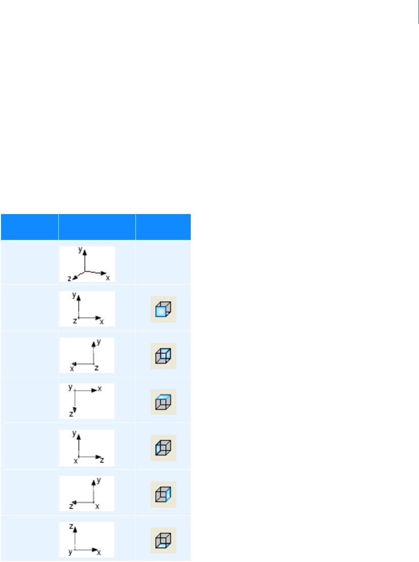
19
Building Plots
Controlling the Display of Three-Dimensional Plots
2. Click the left mouse button on the point in the model that you want at the center of the window.
To return the origin (0,0) of the viewport to the center of the viewport:
On the View menu, point to Position/Orientation, and then select Origin.
Setting the View of Three-Dimensional Plot
Adams PostProcessor provides seven standard views of your three-dimensional plot that you can display. The
table below lists the views, their coordinate system orientations, and the tools on the
Main toolbar that activate
them. You can also redefine the orientations as explained in
PPT Preferences - Orientation.
Standard Views
You can
display the:
The default
orientation is:
Its tool is:
Plot3D No tool
Front
Back
To p
Left
Right
Bottom
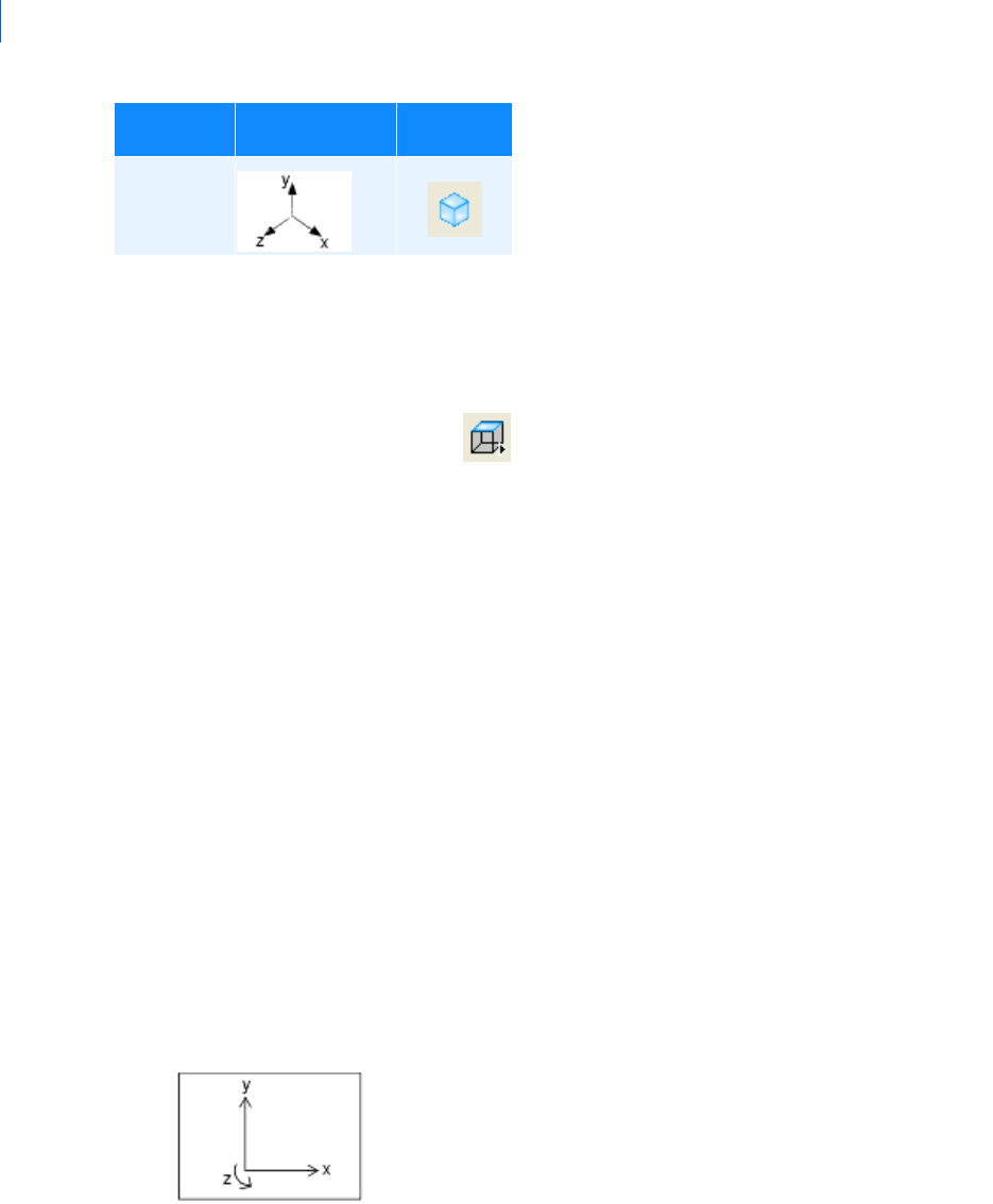
Adams PostProcessor
Controlling the Display of Three-Dimensional Plots
20
To set a view in a viewport:
1. Click the viewport you want to change.
2. Do one of the following:
• On the View menu, point to Pre-Set, and then select a view.
• On the Main toolbar, right-click , and then select one of the View Orientation tools.
Displaying Coordinates of Vertex in Three-Dimensional Plots
To display the coordinates of a vertex in a three-dimensional plot:
Switch to Probe Mode.
To display the coordinates of a vertex on a three-dimensional plot:
Type a lowercase p.
Place the cursor over the vertex of interest.
Adams PostProcessor displays the coordinates (x, y, z values).
Rotating and Translating the Viewport of Three-Dimensional Plot
You can:
Dynamically translate a viewport - You can move the display of a three-dimensional plot in the
viewport so that you can see objects that are outside its boundaries. Translating the view moves the
view in the x, y, and z directions as you move the cursor.
Dynamically rotate a viewport - You can rotate the display of the viewport about any of the view's
three axes (x, y, or z). All the rotation operations work using screen axes. Screen axes are fixed with x
to the right, y up, and z out of the screen as shown below.
Screen Axes
Isometric
You can
display the:
The default
orientation is: Its tool is:
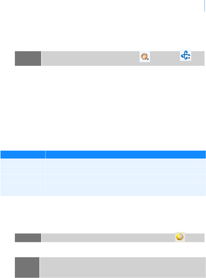
21
Building Plots
Controlling the Display of Three-Dimensional Plots
To dynamically translate or rotate the view:
1. On the View menu, point to Position/Orientation, and then select one of translation or rotation
commands.
2. Place the cursor in the viewport and click and hold down the left mouse button.
3. Drag the cursor in the window in the direction you want to translate or rotate the view. The view of
the window follows the movement of the mouse.
4. When the window contains the desired view, right-click.
Setting Rendering Mode of Three-Dimensional Plots
Adams PostProcessor provides four rendering modes in which you can display a three-dimensional plot in a
viewport, as listed in the table below.
Rendering Modes
To select a rendering mode:
1. Click the viewport whose rendering mode you want to change.
2. On the View menu, point to Render Mode, and then select a rendering mode.
Tip: On the Main toolbar, right-click either Translate XY or Rotate XY , and
then select a tool.
The mode: Does the following:
Wireframe Shows only the edges of objects so that you can see through the objects.
Shaded (flat) Shaded, but polygon edges are visible.
Smooth shaded Shaded, with polygon edges not visible.
Hidden-line removal Shows only the edges of object. It does not show edges, or portions of edges, that
are obscured by other geometry.
Tip: To toggle between shaded and wireframe, on the Main toolbar, select .
Note: If you are using the Native Open GL graphics driver, which is the default, only two
modes have an effect: wireframe and smooth shaded. For more information on
selecting graphics drivers, see
Running and Configuring Adams.
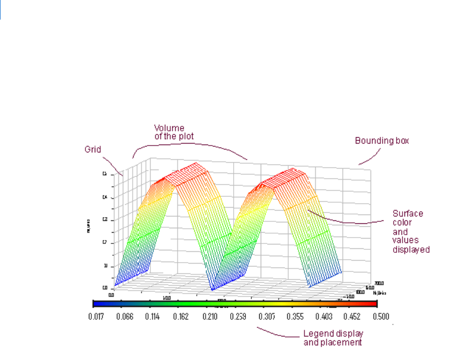
Adams PostProcessor
Controlling the Display of Three-Dimensional Plots
22
Setting Up Three-Dimensional Plot Parameters
The figure below shows the plot parameters that you can set for the general aspects of the three-dimensional
plot, the plot surface colors, and the legend that appears when you select to display a plot as a range of colors
as shown below.
To set general parameters for a three-dimensional plot:
1. Select a three-dimensional plot.
2. In the
Property Editor, clear the selection of:
• Bounding Box to turn off the display of the box surrounding the plot.
• Grid to turn off its grid.
3. In the Graph Volume text box, enter the x,y, and z aspect ratio of the plot. For example, a volume of
1,1,1 makes the plot look like a cube, while a volume of 2,1,1 makes the plot twice as long in the x
dimension as it is in the y and z. See
Example of Same Data with Different Graph Volumes.
To set parameters for the surface of the plot:
1. Select the surface of a three-dimensional plot.
2. In the Skip X or Skip Y text boxes, set the x and y increment of values you want Adams PostProcessor
to skip. Setting it to 1 for creates a smooth surface.
3. Set how you want the colors displayed:
23
Building Plots
Controlling the Display of Three-Dimensional Plots
• To display the surface of the plot as a range of colors, select Interpolated Colors. Then, in the
Number of Colors text box, enter the number of interpolated colors to be displayed in the plot.
There can be no more than 255.
A legend explaining the colors and the values they represent appears. See
Property Editor - 3D Legend
for more information.
• To display the plot as a single color, clear the selection of Interpolated Colors, if necessary, and
set Color to the desired color.
To set parameters for the interpolated color legend of the plot:
1. Set the plot surface to be displayed in interpolated colors as explained above.
2. Select the legend.
3. To turn off the legend, clear the selection of On.
4. Set Legend Placement to where you'd like the legend to appear.
5. In the Number of Colors text box, enter the number of interpolated colors to be displayed in the plot.
There can be no more than 255.
6. In the Gradients text box, enter the number of color gradients shown in the legend
7. Set the properties for the numbers as explained in the table below.
Legend Number Options
To set: Do the following:
Trai l i n g z e r o s Select to have Adams PostProcessor display zeros after the numbers in the legend.
The number of zeros depends on the number of decimal places you selected as
explained next.
Decimal places Enter the number of decimal places to which the numbers in the legend should be
displayed.
Scientific range Enter the exponential form for scientific notation.
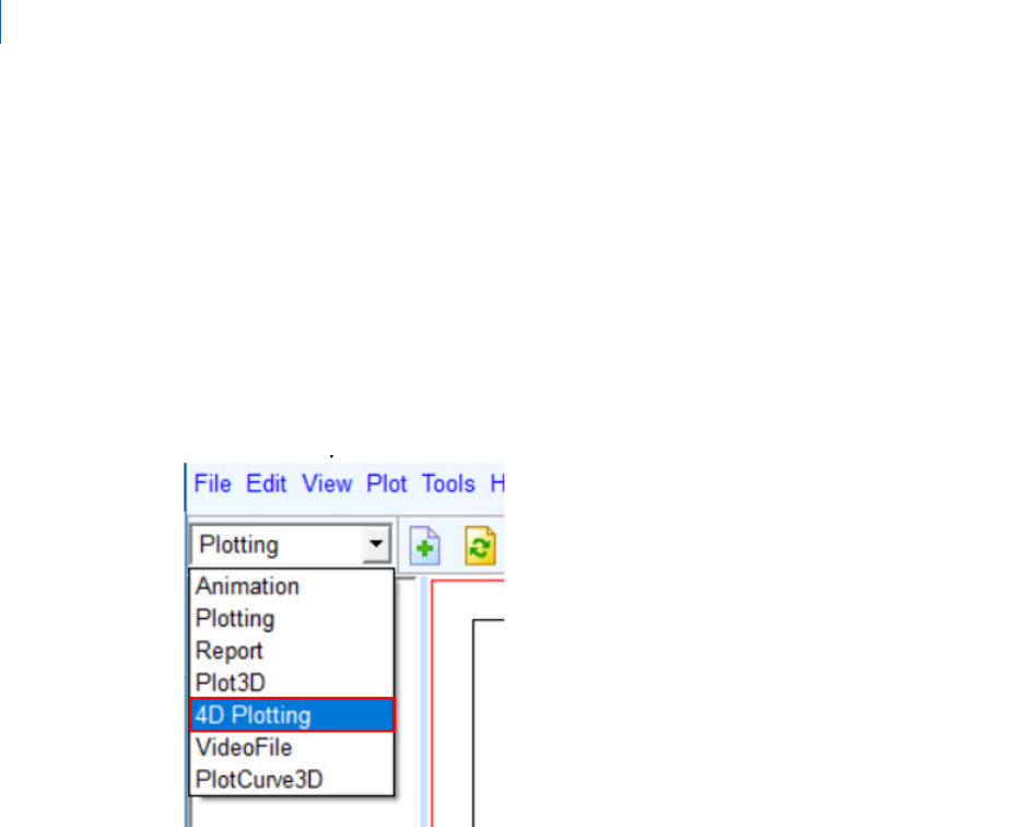
Adams PostProcessor
Building 4D Plots
24
Building 4D Plots
4D Plotting Basics
How to Choose 4D Plotting Mode
There are a number of ways to specify that an Adams Postprocessor window view be designated for 4D
plotting.
Choose "4D Plotting" mode from options available in Adams Post Processor
Right mouse click and select the context menu option "Load 4D Plot" on any of panes in Adams
Post Processor
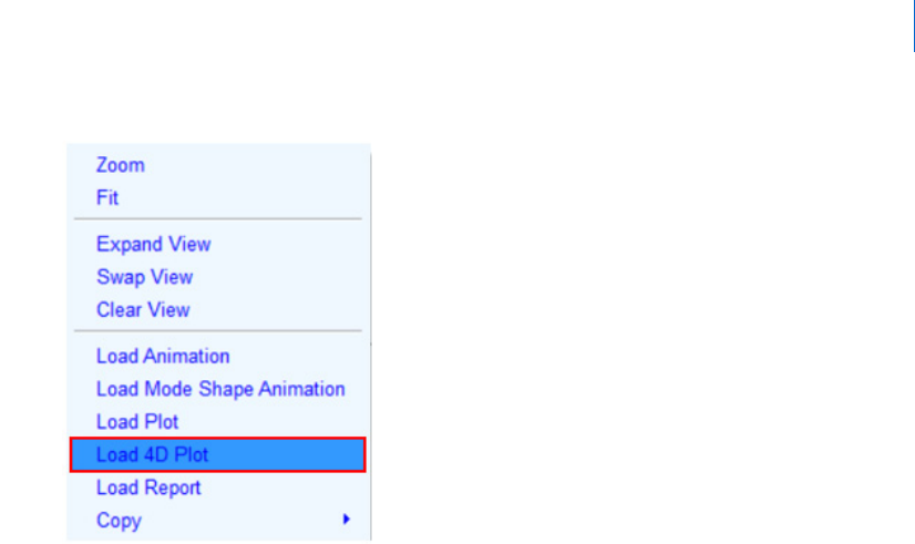
25
Building Plots
Building 4D Plots
Use the Adams View Command Language:
interface plot window set_mode mode = plot4d
Learn more about
Adams View Command Language.
What is a 4D Plot
General 3D Plotting is basically meant for visualizing results by defining a surface in three-dimensional space
with X, Y and Z values, where color interpolation is done based on minimum and maximum values of Z.
The term "4D Plotting" comes from the ability to add another dimension whereby the surface color can,
itself, be an independent parameter and can be plotted based on a different result channel.
Types of 4D Plots
There are two combinations of data types which are supported for 4D Plot creation.
1. Result vs Time across Analyses
This combination helps in analyzing a particular result set component across multiple analyses.
That is, the result set component of interest is the Z axis data (or "height" of the surface/curves) and the X
and Y axes are time and analyses (in either order). Finally, one can choose to color the surface based on the Z
axis data values or based on the values of another result set component.
To summarize the allowable axis combinations:
X axis: Time / Analyses
Y axis: Time / Analyses
Z axis: Result set component
Color: Result set component

Adams PostProcessor
Building 4D Plots
26
Note that the set of analyses chosen must have the same time characteristics (that is, same start and end time,
and same output step sizes).
2. Results vs Time across Fixed values
This combination is meant to plot different result set components across fixed values. That is, a result set
component for each user-specified fixed value. The fixed values would have some meaning of significance to
each of the corresponding result set components. The user will specify the mapping of fixed values to result
set components. A common application is mapping load or motion results to locations in the model. For
example, results for loads along a shaft might be organized using fixed values defining the relative position on
the shaft.
So, the result set component of interest is the Z axis data (or "height" of the surface/curves) and the X and Y
axes are time and fixed values (in either order). Finally, one can choose to color the surface based on the Z
axis data values or based on the values of another result set component.
To summarize the allowable axis combinations:
X axis: Time / Fixed values
Y axis: Time / Fixed values
Z axis: Result set components
Color: Result set components
Note that if result set components are chosen coming from different analyses, those analyses must have the
same time characteristics (that is, same start and end time, and same output step sizes).
4D Plot Rendering options
There are three different ways by which data can be rendered with 4D plotting: as a surface, as stacked curves
or as a Color Map.
1. Surface
With the surface option, the data is rendered as a geometrical surface mesh. The colors are interpolated
between the actual result points (the "nodes" of the surface's geometrical mesh). Note that in order to render
this surface the number of Z values must equal the number of X*Y values.
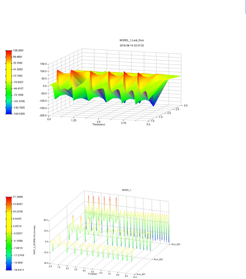
27
Building Plots
Building 4D Plots
2. Stacked Curves
With the stacked curves option the data are rendered as a series of 2D polylines, one for each 2D curve in the
Z-X or Z-Y plane. This rendering option is particularly useful when one does not want to infer any
conclusions about the results between curves. Note that in order to render this surface the number of Z values
must equal the number of X*Y values.
3. Color Map
If the Z Axis checkbox is not selected, a surface will not be generated. The data will be rendered as a 2D color
map, where the color values come from the specified result set components.
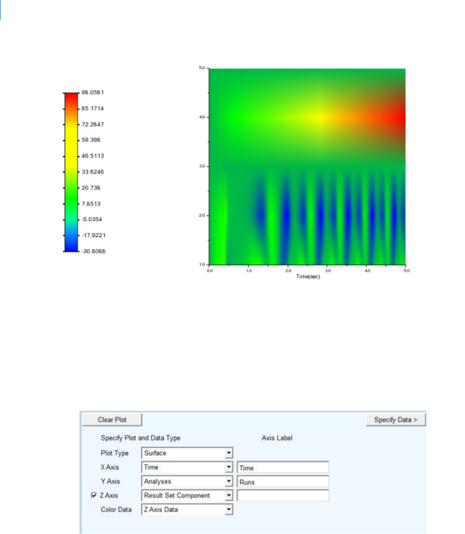
Adams PostProcessor
How to Create 4D Plots
28
How to Create 4D Plots
The sections below describe how to create 4D Plots of each type and employing each of the rendering options.
Result vs Time across Analyses
1. Start by selecting the Analyses option from either the X or Y axis option menu and optionally specify
text for the labels of the X and Y axes.
2. Next click the "Specify Data" button.
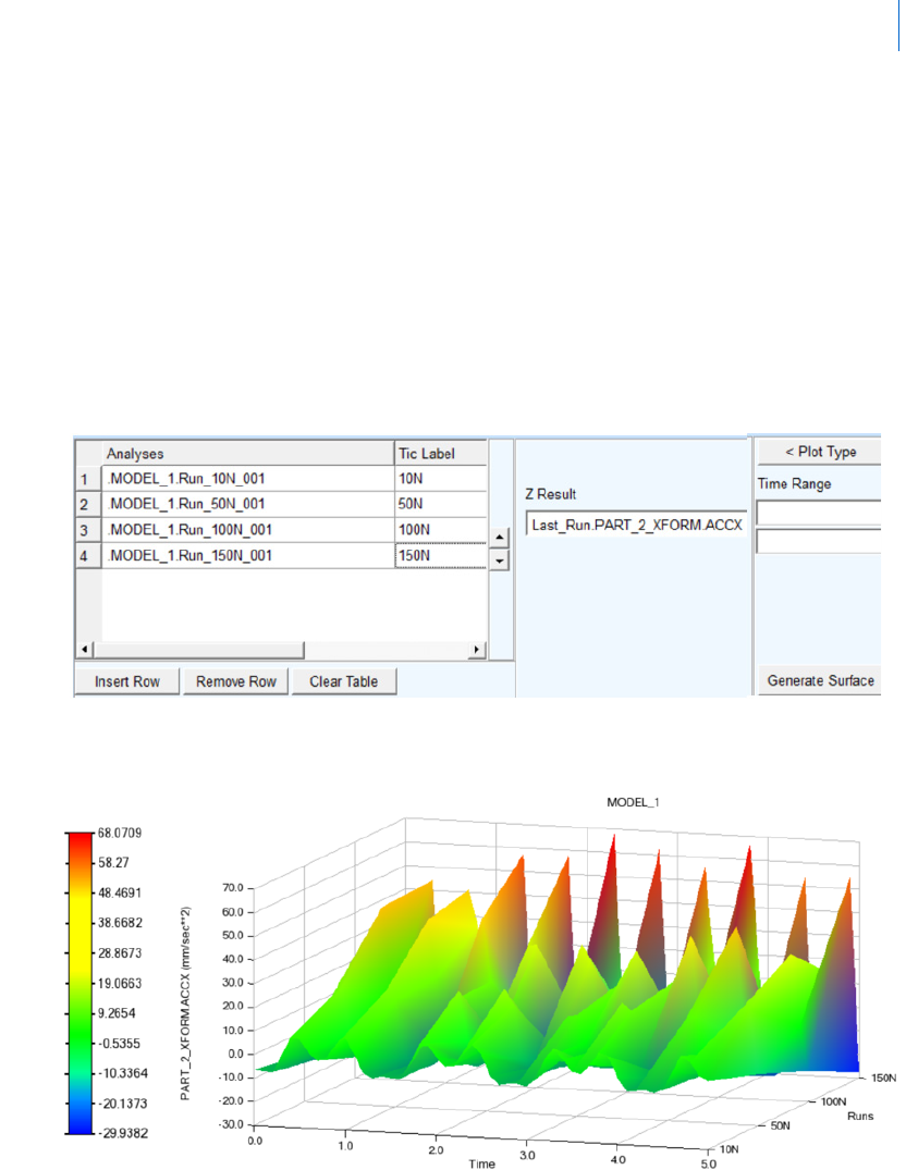
29
Building Plots
How to Create 4D Plots
3. The next page, the Specify Data page, has a table to populate with the set of analyses to be used and
it has fields in which to specify the result sets to be used for the values of the Z-axis and, if chosen on
the Plot Type page, the surface color.
4. Select multiple analyses from the database navigator using the context menu via clicking the right-
mouse button from within the first column of the data table.
5. In the second column one can specify the tic label to be used for each of the analyses. If left blank the
short name of analyses will be used.
6. Then, in the "Z Result" field, select the result set component to be plotted from each analysis. It does
not matter from which analysis you choose this result set component. This same result set component
will be plotted from each of the analyses in the table.
7. Finally, click "Generate Surface" and the Plot will be created:
Independent Surface Color
In the above example, the color interpolation is done based on the Z result set component (that is, the
"height" of the surface).
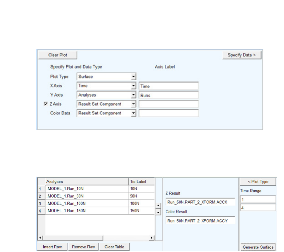
Adams PostProcessor
How to Create 4D Plots
30
To plot color as separate component, set "Color Data" to "Result Set Component" as follows:
Then, the Specify Data page will present an additional field for "Color Result" field from which an result
component can be selected.
Time range can be used to plot a data within values of interest.
Then, if you click Generate Surface the surface color will be based upon the result set component in "Color
Result." Also notice that the color legend gets an independent label.
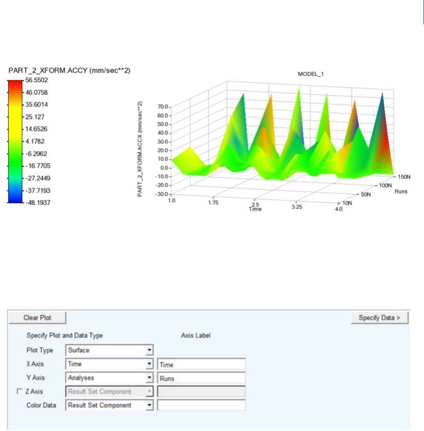
31
Building Plots
How to Create 4D Plots
Color Map
In the examples above, the data is rendered as a 3D surface. To plot the data as a 2D color map, a Z axis is
not required. To achieve this, uncheck the "Z Axis" option and set Color Data to "Result Set Component"
as follows:
Then, the Specify Data page will present only the "Color Result" field from which a result component can
be selected.
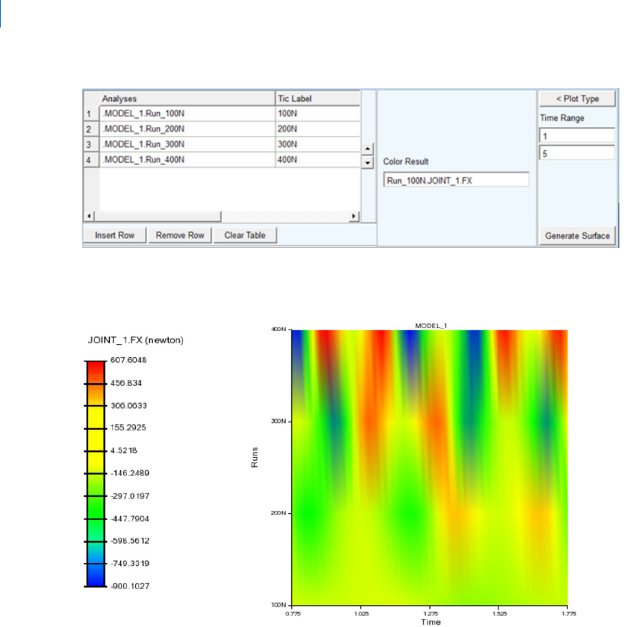
Adams PostProcessor
How to Create 4D Plots
32
Then, if you click Generate Surface, the 2D Color Map will be generated with color values based upon the
result set component specified in the "Color Result" field with a corresponding legend.
Sequence of Analyses
With the arrow buttons provided in analyses data table, analyses can be re-arranged in upward and downward
directions with up and down arrows.
For example, analysis for 150 N has been shifted upwards to the second position.
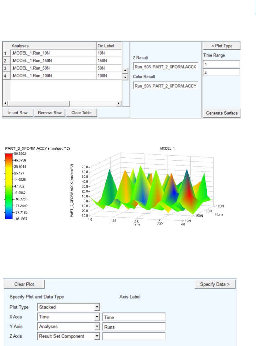
33
Building Plots
How to Create 4D Plots
Now, "Generate Surface" will create the surface according to this sequence of analyses.
Using Stacked Curves
To plot the data in the form of stacked curves go to the Plot Type page and set Plot Type to "Stacked" as show
below. Then, proceed through the Specify Data page to generate the plot.
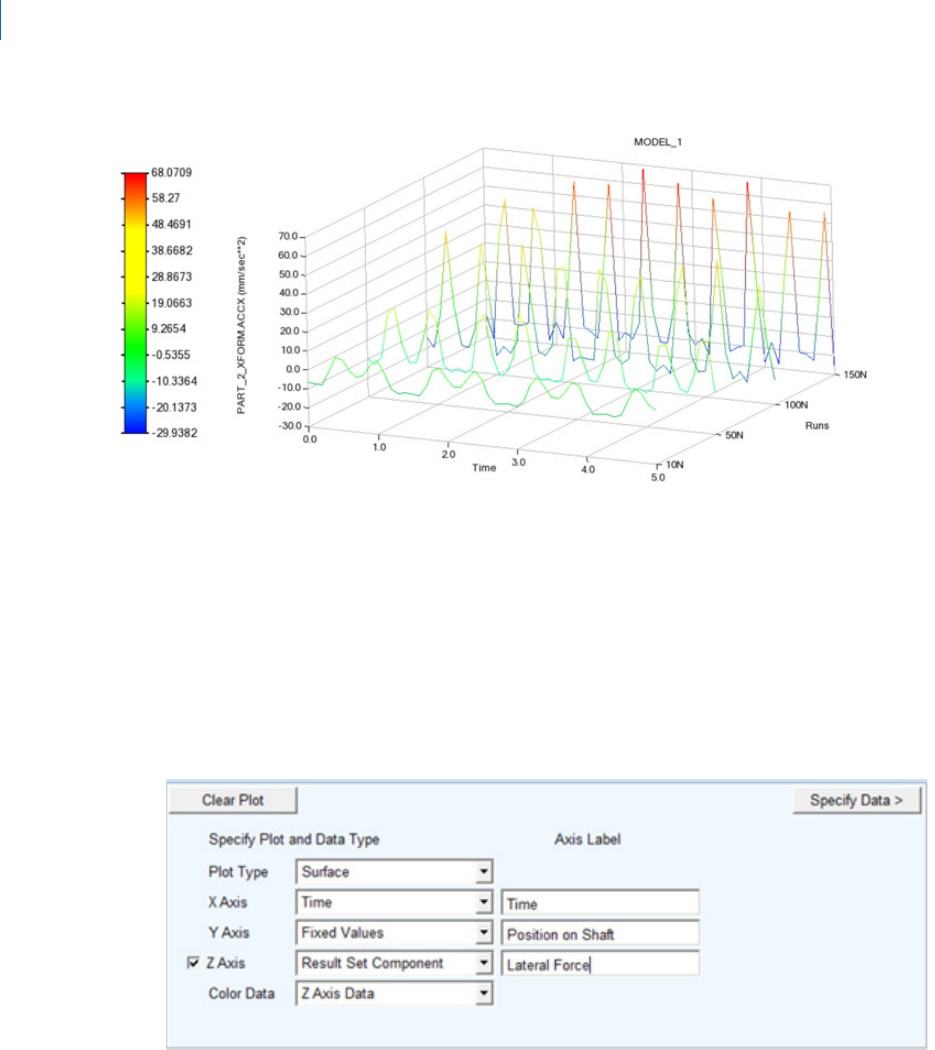
Adams PostProcessor
How to Create 4D Plots
34
Note that when Stacked curves option is selected, color cannot be set independently. This is supported only
for the "Surface" plot type option.
Result vs Time across Fixed Values
1. Start by selecting the Fixed Values option from either the X or Y axis option menu and optionally
specify text for the labels of the X and Y axes.
For example, the Fixed values could represent physical locations at which the model is instrumented
and, therefore, a result component is present in analysis for each.
2. Next click the "Specify Data" button.
The next page, the Specify Data page, has a table to populate with the mapping of Fixed Values to
Result Set Components.
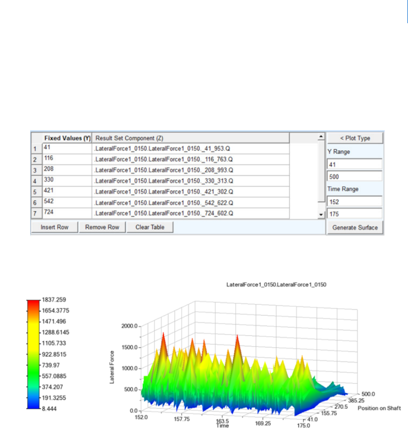
35
Building Plots
How to Create 4D Plots
3. Select multiple analyses from the database navigator using the context menu via clicking the right-
mouse button from within the second column of the data table. Multiple components can be selected
and it will result in as many rows as is required to accommodate all selected components. If
components are already present in those cells then these will be replaced.
4. Time range and data range can be used to plot data within values of interest.
5. Finally, click Generate Surface to create the plot:
Independent Surface Color
In the above example, the color interpolation is done based on the Z result set component (that is, the
"height" of the surface).
1. To plot color as separate component, set "Color Data" to "Result Set Component" as follows:
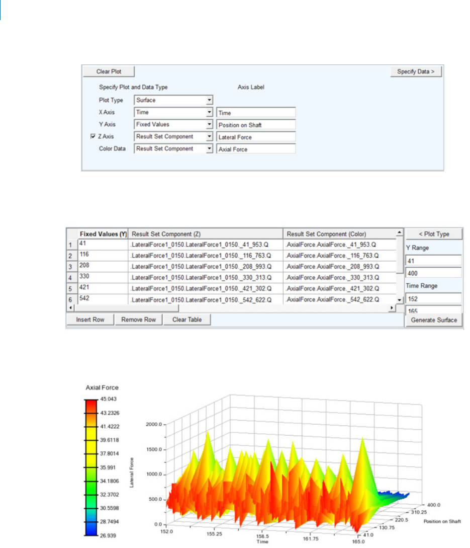
Adams PostProcessor
How to Create 4D Plots
36
2. Once Color Data has been selected as "Result Set Component", the data table on the Specify Data
page will have another column in which result set components for color can be chosen.
3. Then, if you click Generate Surface the surface color will be based upon the result set component in
"Color Result." Also notice that the color legend gets an independent label.
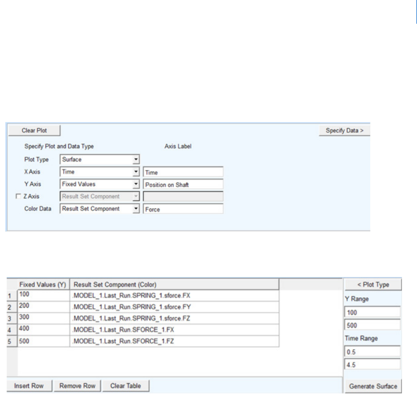
37
Building Plots
How to Create 4D Plots
Color Map
In the examples above, the data is rendered as a 3D surface. To plot the data as a 2D color map, a Z axis is
not required. To achieve this, uncheck the "Z Axis" option and set Color Data to "Result Set Component"
as follows:
The Specify Data page will have a column for color result set components only.
Then, if you click Generate Surface, the 2D Color Map will be generated with color values based upon the
"Result Set Component (Color)" column.
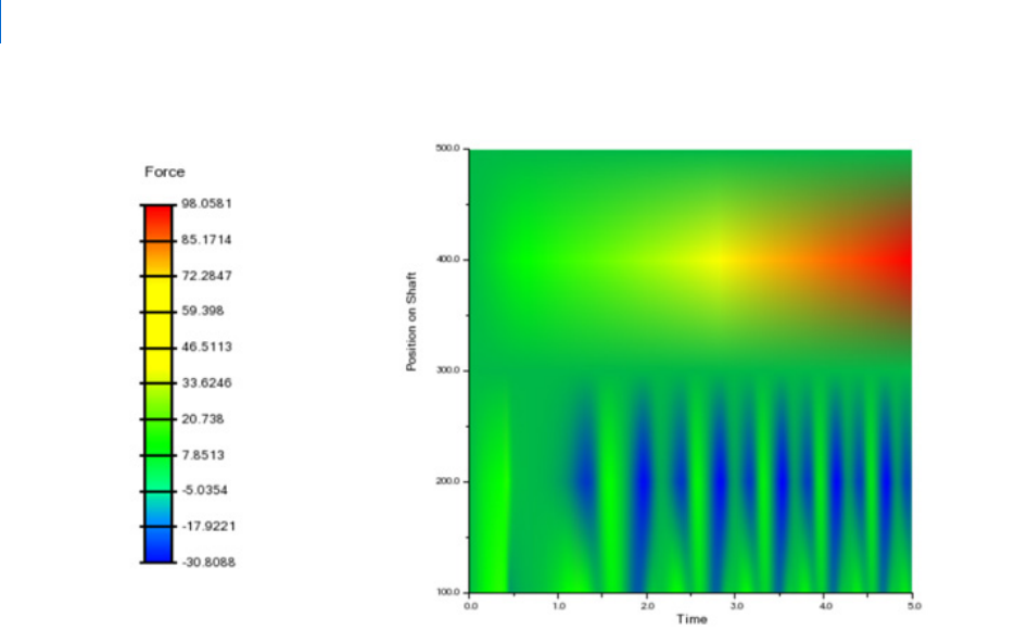
Adams PostProcessor
Modifying 4D Plots
38
Modifying 4D Plots
Modification can be done in two ways:
1. Dashboard: Once a 4D plot has been created, when it is selected again, the plotting dashboard will
be in modify mode. Note that X/Y axis combinations can't be changed in modify state, but one is
allowed to change the plot type, toggle the color data option and edit the contents of the Data page
2. Property Editor: Similar to modification of 2D XY plots, the property editor (situated beneath the
tree view in Adams Post Processor) can be used to edit aspects of the plot display but not its data
39
Building Plots
Modifying 4D Plots
Property Editor - 4D Plot
In tree view → page → 4D plot
Property Editor - 4D Surface
In tree view → page → 4D plot → surface_3d
For the option: Do the following:
Bounding Box Clear to turn off the display of the three-dimensional box surrounding the
plot.
Grid Select [Off/Clear/Shaded]
Off- No grid
Clear- Normal grid with lines
Shaded - Grid with shaded background
Graph Volume Enter the x, y, and z aspect ratio of the plot. For example, a volume of 1,1,1
makes the plot look like a cube, while a volume of 2,1,1 makes the plot twice
as long in the x dimension as it is in the y and z.
For the option: Do the following:
Skip X/Skip Y Set the x and y increment values you want Adams PostProcessor to skip.
Setting it to 1 for each creates the smoothest surface.
Interpolated Colors Select to display the surface of the plot as a range of colors. A legend explaining
the colors and the values they represent appears.
Color Set the single color with which to display the surface.
Number of Colors Enter the number of interpolated colors to be displayed in the plot. There can
be no more than 255.
Style Select either of options. [Surface, Stacked]
Stacked option will convert surface into stacked curves with polylines.
Default is surface.
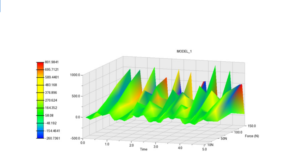
Adams PostProcessor
Animation of 4D Plots
40
Example of Shaded Grid 4D Plot
Animation of 4D Plots
4D Plots can be animated with both the Time Marker and Advancing Surface animation options as described
in
Animating Results.
Animation Type
This option determines how the plot's curve(s) will be drawn as time moves forward. It has the following two
options:
Advancing Curve: Includes a sub-option "Time Window (sec)" by which a moving window of time can
be specified (for example, display on the last 5-seconds of time). Plot's curve(s) and 4D plot surface will
be drawn in a way where h-axis has range of values equivalent to time window, if specified, and
curve/surface will be displayed in accordance with time value.
Time Marker: Plot's curve(s) will be displayed as per the axes' limits. In addition, a vertical line with a
symbol tracing the curve's value at a particular will be displayed at a given frame. In case of 4D Plot, a
line across time axis will be displayed at each time step.
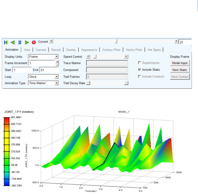
41
Building Plots
Animation of 4D Plots
Time Marker Animation with 4D Plot
At a given time step, a time line will be displayed as follows.
In case of 2D color map, vertical line will be displayed as "Time Marker" at a given time.
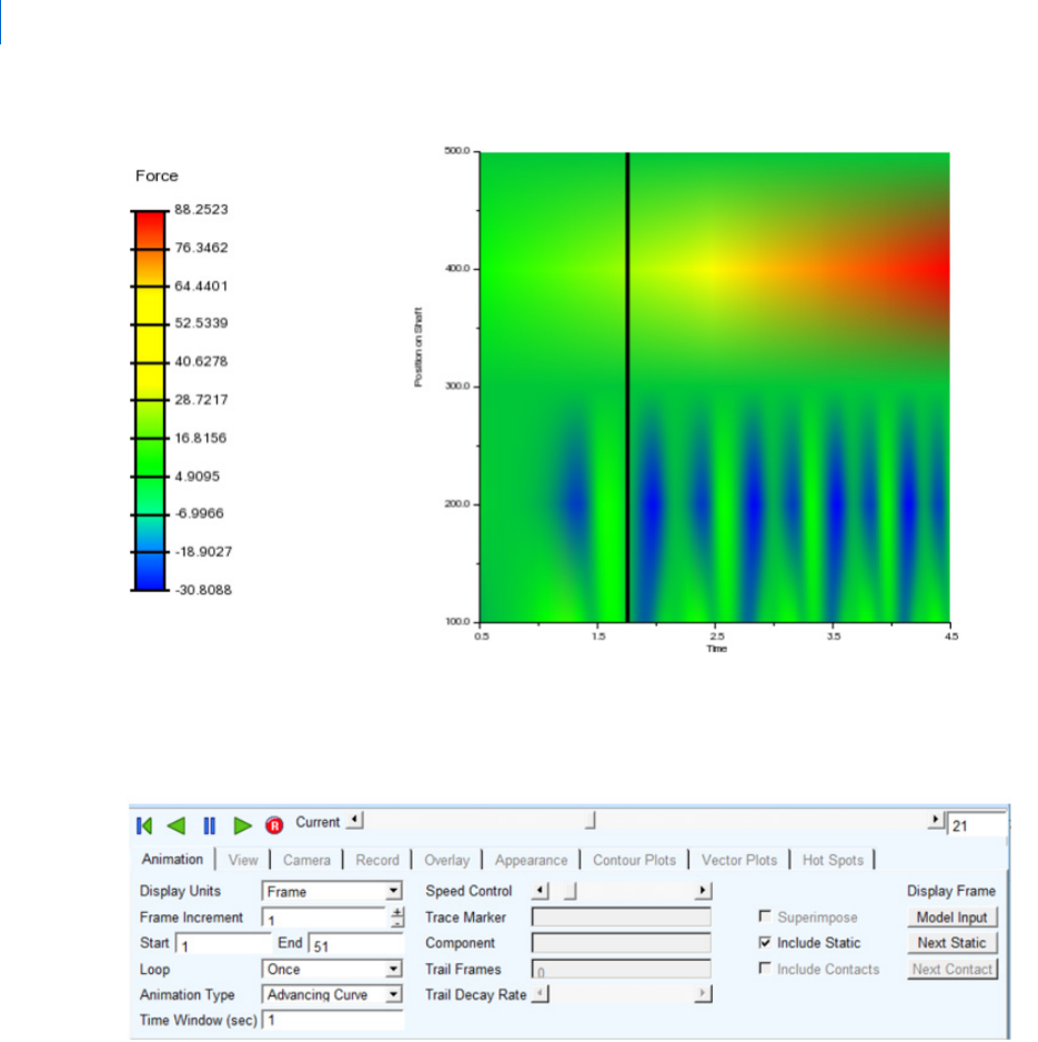
Adams PostProcessor
Animation of 4D Plots
42
Advancing Surface Animation
Time window of 1 sec has been used to analyze results as follows.
Intermediate stage having time values of 1-2 range has been shown during animation.
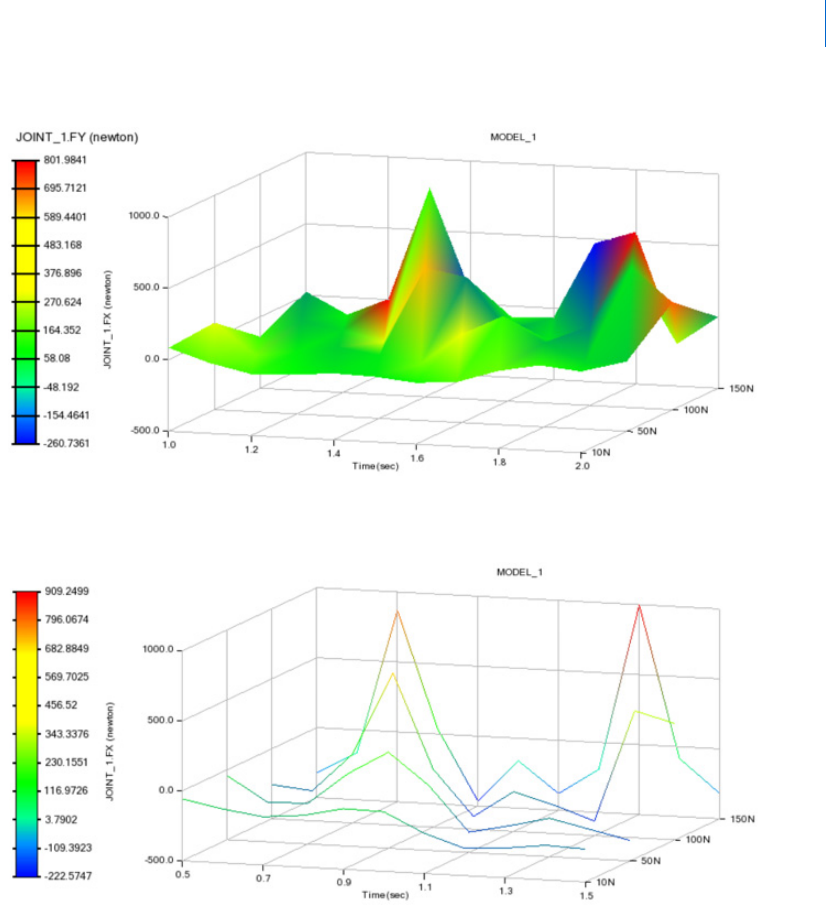
43
Building Plots
Animation of 4D Plots
Advancing animation can be done in stacked curves mode also as follows:
Advancing animation with 2D color map will be displayed as follows:
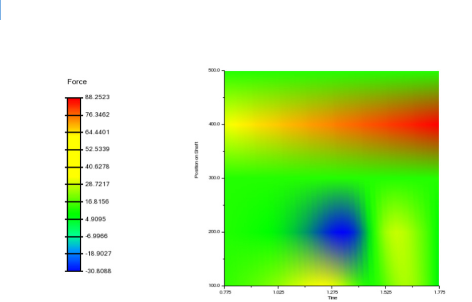
Adams PostProcessor
Controlling the Display of 4D Plots
44
Controlling the Display of 4D Plots
These controls are the same as for 3D plotting (for example, in Adams Vibration and 3D FFT). There are no
differences with regards to arrangement of views and view manipulation (like rotate, zoom and so on). See
"
Controlling the Display of Three-Dimensional Plots" for details.

45
Building Plots
4D Plotting via the Plot Configuration File
4D Plotting via the Plot Configuration File
4D Plots can be saved in a plot configuration file (.plt) like 2D XY plots. See Plot Configuration Files for more
information.
Format
Examples illustrating the format of the plot configuration file content when exporting a 4D Plot are shown
below.
Result Set Components vs Time across Fixed Values:
[PLOT4D_SURFACE]
NAME = 'surf3d_1'
PLOT4D = 'plot3d_1'
INTERP_COLORS = 'on'
STACKED = 'no'
X_DATA = 'Time'
Y_DATA = 'Fixed_Values'
FIXED_VALUES = '1.000000,2.000000,3.000000,4.000000'
Z_DATA = 'JOINT_1.FX,JOINT_1.FY,JOINT_1.TX,JOINT_1.TY'
COLOR_DATA =
'PART_2_XFORM.ACCX,PART_2_XFORM.ACCY,PART_2_XFORM.PHI,PART_2_XFORM.PSI'
Result Set Components vs Time across Analyses:
[PLOT4D_SURFACE]
NAME = 'surf3d_1'
PLOT4D = 'plot3d_2'
INTERP_COLORS = 'on'
STACKED = 'no'
X_DATA = 'Time'
Y_DATA = 'Analysis'
Z_DATA = 'JOINT_1.FX'
COLOR_DATA = 'JOINT_1.FY'
Importing .plt Files with 4D Plots
When importing a plot configuration file (.plt) containing 4D Plots, there a number of scenarios to consider
with regards to the content of the originally created 4D Plots and the options on the .plt file import dialog,
especially with regard to the number of analyses in each.
Adams PostProcessor
4D Plotting via the Plot Configuration File
46
Number of
Analyses Involved
in Original Plot
One Analysis Provided During .plt
Import
Multiple Analyses Provided During .plt Import
X&Y (Fixed
Values, Time)
Z&Color (Result
Set Component)
X&Y (Analyses,
Time)
Z&Color (Result
Set Component)
X&Y (Fixed Values, Time)
Z&Color (Result Set
Component)
X&Y (Analyses,
Time)
Z&Color (Result Set
Component)
1 4D plot will be
created replacing
original analysis
used during
creation with
analysis specified
during .plt import.
If any of the result
set components
don't exist in the
specified analysis,
then this plot will
be skipped.
N/A
(this scenario
requires minimum
two analyses)
For each analysis specified
upon import, separate 4D
plots will be created by
maintaining the original fixed
value -to- result set component
mapping with the imported
analysis.
If any of the result set
components don't exist in any
of the new analyses, then this
analysis will be skipped and
next analysis will be considered
in plot generation.
Cross-Plotting is not
supported for 4D plots; so,
individual 4D plots will be
made for each analysis if this
option is chosen.
N/A
(this scenario requires
minimum two
analyses)
47
Building Plots
4D Plotting via the Plot Configuration File
2 or more All the original
analyses will be
replaced with the
one specified upon
.plt import and a
warning will be
issued.
This plot will be
skipped and an
error message will
be issued.
4D plots composed of fixed
values and multiple analyses
cannot be recreated via .plt
import. This plot will be
skipped and an error issued.
4D plot will be created
by replacing all
original analyses with
the chosen analyses in
.plt import.
If the result set
component doesn't
exist in any of the new
analyses, such an
analysis will be
omitted from the plot
and the plot will
completed with the
remaining analyses.
If none of the new
analyses contain the
result set component,
then an error message
is issued, and this plot
is skipped.
Cross-Plotting is not
supported for 4D
plots; so, individual
4D plots will be made
for each analysis if this
option is chosen.
Number of
Analyses Involved
in Original Plot
One Analysis Provided During .plt
Import
Multiple Analyses Provided During .plt Import
Adams PostProcessor
Modifying Axis Attributes
48
Modifying Axis Attributes
You can change the following about the horizontal and vertical axes of two-dimensional plots and the x, y,
and z axes of three-dimensional plots:
Modifying Axes Format
Modifying Tic Marks
Modifying Axis Labels
Modifying Axis Numbers
Modifying Axes Format
By default, Adams PostProcessor automatically scales the axes in a plot based on the curves. You can change
the default values.
To modify the format of the horizontal or vertical axis:
1. Select a horizontal or vertical axis.
2. In the
Property Editor, select Format.
3. Set the scaling for the axis as explained in the table below.
Scaling Options
To: Do the following:
Automatically calculate
the scaling
Select Auto Scale. You can specify that Adams PostProcessor automatically set
the minimum and maximum values or your can set them manually. By
manually setting minimum and maximum values for the axis, you can zoom
in on different areas of your plot. For example, to view the values between 0
and 10, you can set the minimum value to 0 and the maximum value to 10.
Adams PostProcessor then only displays the values between these numbers in
your plot.
Use the current time
range as the axis limits
Select Auto Time Limits.
Set the time limits Clear Auto Time Limits and enter the time limits for the axis in the two Time
Limits text boxes that appear. Enter the minimum value in the first box and
the maximum value in the second box.
Note: Setting time limits is only useful when working with the
independent (horizontal) axis.
For linear- and dB-scaled axes, enter lower and upper limits. For
logar-scaled axes, enter log base 10 for lower and upper limits. (See
scaling options below.)

49
Building Plots
Modifying Axis Attributes
4. Set Scale to the type of scaling. By default, Adams PostProcessor displays the axis values linearly,
starting at 0. You can also change the scaling to:
• Logarithmic - Scales the axis values so that each power of 10 is separated by the same distance.
For example, the values 1, 10, 100, 1000, and 10,000 are equally spaced.
• Decibel (dB) - Displays 20 * log
10
(value) for each value.
5. Set Placement to where you want to place the axis. The options available depend on whether you are
modifying the horizontal or vertical axis. You can place an axis on the right or left or at the top or
bottom.
6. In the Offset text box, set how far from the border of the plot you want to display the axis.
7. Set Color to the color for the axis.
Modifying Tic Marks
By default, Adams PostProcessor displays short lines, called tic marks, at regular intervals across the axis. The
tic marks help to define the scale of the axis. Adams PostProcessor displays the major tic marks at every unit
value and the minor tic marks halfway between the major tic marks.
For major tic marks, you can set the spacing by setting:
Increments - Specifies intervals across the axis, such as at every unit value, every second unit value,
and so on, at which tic marks should appear.
Divisions - Divides the axis evenly into a number of segments and places a tic mark at every division.
For minor tic marks, you can set how many minor tic marks appear between each major tic mark.
To modify tic marks:
1. Select a horizontal or vertical axis.
2. In the
Property Editor, select Tics.
3. To turn off automatic divisions, clear the selection of Auto Divisions and select how you want the
major tic marks spaced from the pull-down menu. Enter the number of increments or divisions in
the text box.
4. In the Minor Divisions text box, enter the number of divisions between each major tic mark. The
number of divisions sets the number of minor tic marks. For example, if you set the number of
divisions to two, Adams PostProcessor places one tic mark between each major tic mark.
5. Set Color to the color for the tic marks.
Modifying Axis Labels
By default, Adams PostProcessor displays a label next to an axis to help identify the values in the axis. The
label identifies the unit of measurement in the axis. You can change the text of the label, its placement, font
size, and color.
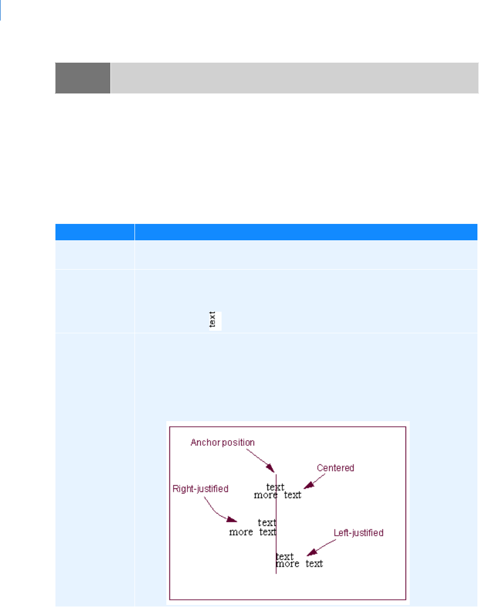
Adams PostProcessor
Modifying Axis Attributes
50
To modify axis labels:
1. Select a horizontal or vertical axis.
2. In the
Property Editor, select Labels.
3. In the Label text box, enter the text for the label.
4. Set the properties for the axis label as explained in the table below.
Axis Label Options
Note: You can also modify the label text using the instructions in Adding Notes and Modifying Text, which
allows you to create multi-line labels.
To set: Do the following:
Size of the text In the Font Size text box, enter a font size. The font size you can enter depends on the
type of font you selected.
Orientation of the
text
Select either:
Horizontal - text
Vertical -
Alignment Select how you want the label to be aligned relative to its anchor position, which is the
center of the text. See the figure below. You can select:
Left - Left-justifies the text from the anchor position.
Center - Centered the text on its anchor position.
Right - Right-justifies the text from the anchor position.
51
Building Plots
Additional Topics
Modifying Axis Numbers
By default, Adams PostProcessor displays numeric values for an axis at each major increment. You can change
the way in which Adams PostProcessor displays the values, such as the number of decimal places displayed
and whether or not Adams PostProcessor uses scientific notation.
To modify axis numbers:
1. Select a horizontal or vertical axis.
2. From the
Property Editor, select Numbers.
3. Set the properties for the axis numbers as explained in the table below.
Axis Number Options
Additional Topics
Setting Curve Properties
You can specify properties for curves as explained below. You can also set defaults for how Adams
PostProcessor creates curves, as explained in
PPT Preferences - Curves.
Color Set Color to the color for the text.
Location Clear the selection of Auto Position and, in the Offset text box, enter an offset value
to define the distance the label is offset from the border of the plot.
To set: Do the following:
Trai l i n g z e r o s Select Trailing Zeros to have Adams PostProcessor display zeros after the numbers in
the axis. The number of zeros depends on the number of decimal places you selected
as explained next.
Decimal places In the Decimal Places text box, enter the number of decimal places to which the
numbers in the axes should be displayed.
Scientific range In the Scientific Range text boxes, enter the exponential form for scientific notation.
Font size In the Font Size text box, enter a font size. The font size you can enter depends on
the type of font you selected.
Color Set Color to the color for the numbers.
To set: Do the following:
Note: In addition to setting a curve's properties, you can edit the data in the curves. Learn about
performing calculations on curves
.
Adams PostProcessor
Additional Topics
52
To modify the properties of a curve:
1. Select a curve.
2. In the
Property Editor, set the properties for the curve as explained in the table below.
Curve Property Options
To set: Do the following:
Text f o r l e g e n d In the Legend text box, enter the text to appear in the legend associated with this
curve. Adams PostProcessor displays the legend with a short line segment
illustrating the color and line style of the curve. If you updated your plots, Adams
PostProcessor creates a second legend, called the simulation legend. You modify the
simulation legend text separately. For more information on modifying legends, see
Modifying Legend Properties. For more information on the types of legends, see Updating
Plot Data
.
Note: You may want to expand the width of the Property Editor so you have
more space for entering the legend text. To expand the property editor,
point to its right border. When the cursor changes to a double-sided
arrow, drag the cursor to increase the property editor's size.
Color Set Color to the color for the curve.
Line style and
weight
Select the type of line style and weight for the curve. The weight values range from
1 to 5 screen pixels. You can also set the line style to None so that Adams
PostProcessor does not display the curve line. If you selected to display symbols
along the curves, the symbols still appear when you turn off the curve line. The
effect is a scattered plot.
Symbol and symbol
increment
Select the type of symbol that you want at data points along the curve and select
how often you would like the symbol to be displayed along the curve.
53
Building Plots
Additional Topics
Modifying Legend Properties
You can change the placement and border of legends on your plots. There are two types of legends in Adams
PostProcessor:
Curve legend text that describes the data that each curve on the plot represents.
If you update your plot data, as explained in Updating Plot Data, Adams PostProcessor creates a second
legend, called the simulation legend. The simulation legend contains groups of text that describe the
data in a specific simulation.
This procedure does not let you change the text of legends.
Learn about changing curve legends.
You also cannot change the legend when a plot is displayed as a table.
Learn about displaying plots as tables.
To modify legend properties:
1. Select a legend.
2. In the
Property Editor, turn on the legend.
3. Set the properties for the legend as explained in the table below.
Plot Legend Property Options
Hotpoints You can turn on hotpoints that let you manually edit the data points in the curve.
You can also control how you edit the hotpoints, only vertically or only horizontally,
so you have greater control. For more on hotpoints and manually editing curves, see
Manually Changing Data Point Values.
Select one of the following:
Off - To have no hotpoints displayed.
On - Turn on hotpoints, to allow the editing of the data points in any
direction.
Horizontal - Turn on hotpoints, but only allows the editing of the data
points in the horizontal direction.
Vertical - Turn on hotpoints, but only allows the editing of the data points
in the vertical direction.
Note: You can use the
Hotpoints tool on the Curve Edit toolbar to override
this setting.
To set: Do the following:
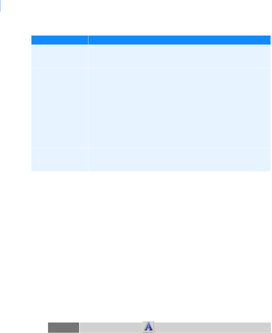
Adams PostProcessor
Additional Topics
54
Adding Notes and Modifying Text
You can add text, called a note, to any area of your plot and set the appearance of the note. For example, you
might want to add a note that points out a trend in a plot or that labels a data point. Once you've created the
note, you can modify it and change its placement by dragging it. You can also modify the text of titles and
subtitles.
Learn about adding notes and modifying text:
Creating Notes
Modifying Text
Moving Text
Creating Notes
You can create notes with one or more lines of text.
To create notes on your plots:
1. From the Plot menu, select Create Note.
To set: Do the following:
Transparency of the
legend
If you want the legend to be transparent, clear the selection of Fill. Any plot
information behind the legend shows through. When you select Fill, the legend
is opaque and covers any information behind it.
Placement of the
legend
Set Placement to any of the following:
Top Right
Top Left
Bottom Left
Bottom Right
Axis - Places the legend text for each legend on the appropriate
dependent axis.
User-placed - Sets the legend so you can move it to any position, as
explained in
Moving Text.
Whether or not the
legend has a border and
the border's style
If you do not want a border around the legend, clear the selection of Border. If
you do want a border, keep Border selected and then select a color, line weight,
and line style for the border.
Tip: From the Main toolbar, select .
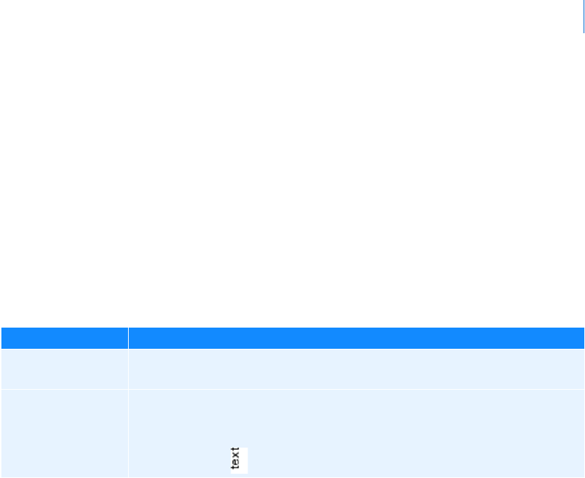
55
Building Plots
Additional Topics
2. Click where you want the note to appear, and enter the text, pressing Enter to create another line of
text.
Modifying Text
You can modify any existing notes, titles, and subtitles.
To modify existing text:
1. Select the text.
2. In the
Property Editor, enter or change the text in the text area. You can enter multiple lines of text.
3. Set the options for the text as explained in the table below.
Label Options
To set: Do the following:
Size of the text In the Font Size text box, enter a font size. The font size you can enter depends on
the type of font you selected.
Orientation of the
text
Select either:
Horizontal - text
Vertical -
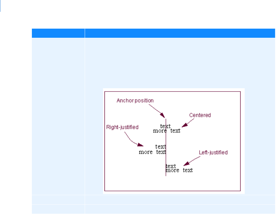
Adams PostProcessor
Additional Topics
56
Moving Text
The following shows how to move the text of notes, titles, subtitles, and legends by dragging it. You can also
position the text precisely using the Property Editor as explained in
Modifying Text.
To move text by dragging it:
1. Select the text.
2. Drag the text in the direction you want to move it.
Adding Spec Lines
You can add spec lines to your plots to help you compare curves to a constant baseline value. A spec line can
be a horizontal, vertical, or diagonal line that indicates a value of significance. You can start the spec line at
any X or Y position.
Alignment Select how you want the label to be aligned relative to its anchor position, which is
the center of the text. See the figure below. You can select:
Left - Left-justifies the text from the anchor position.
Center - Centered the text on its anchor position.
Right - Right-justifies the text from the anchor position.
Color Set Color to the color for the text.
Location Clear the selection of Auto Position and enter a location for the text.
To set: Do the following:
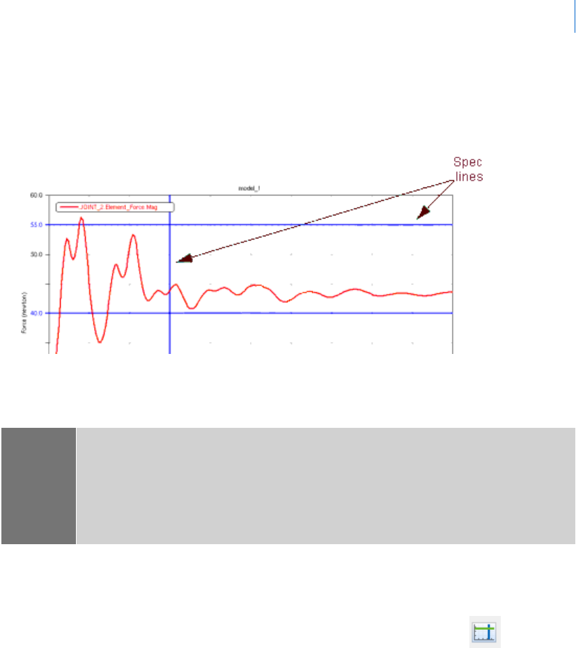
57
Building Plots
Additional Topics
For example, if you are plotting acceleration and you want to keep the acceleration below a certain value, you
can add a spec line marking that value on the plot. You can then compare any curves that you add to that
plot to see if the curves fall beneath the spec line.
The following figure shows spec lines that have been added to a plot.
Example of a Spec Line
There are no limits to the number of spec lines you can add to a plot.
To add a spec line to a plot:
1. Select the plot to which you want to add a spec line.
2. From the Plot menu, select Create Spec Line, or click the Create Spec Line icon in the toolbar.
3. In the Spec Line Name text box, enter the name you want to assign to the spec line. The box shows
the complete name of the spec line, including its parents in the database.
4. In the Y Value and X Value text boxes, enter:
• For a horizontal spec line, enter only a y value.
• For a vertical spec line, enter only an x value.
• For a diagonal spec line, enter both an x and y values.
For example, entering both x and y values, provides the following diagonal spec line:
Notes: If you have turned on plot statistics, you can quickly create a spec line at the current location
of the plot tracking cursor using the keyboard shortcuts:
s or S create vertical spec lines.
h or H create horizontal spec lines.
Learn about displaying plot statistics.
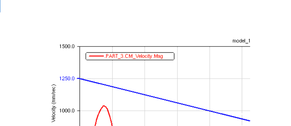
Adams PostProcessor
Displaying Plots as Tables
58
5. Select a color, type of line, and thickness for the line. The thickness values range from 1 to 5 screen
pixels.
6. Select OK.
To modify a spec line:
1. Select the line.
2. In the property editor, set values for the line as explained above for creating a spec line.
Displaying Plots as Tables
To help you better see a two-dimensional plot's numerical information, you can view a plot as an HTML
table. In addition, you can always have your plots display as tables by setting a preference as explained in
PPT
Preferences - Plot
dialog box help. The figure below shows a plot displayed as a table.
Learn more:
Changing a Plot to a Table
Changing Table Properties
Changing Dependent Column Properties
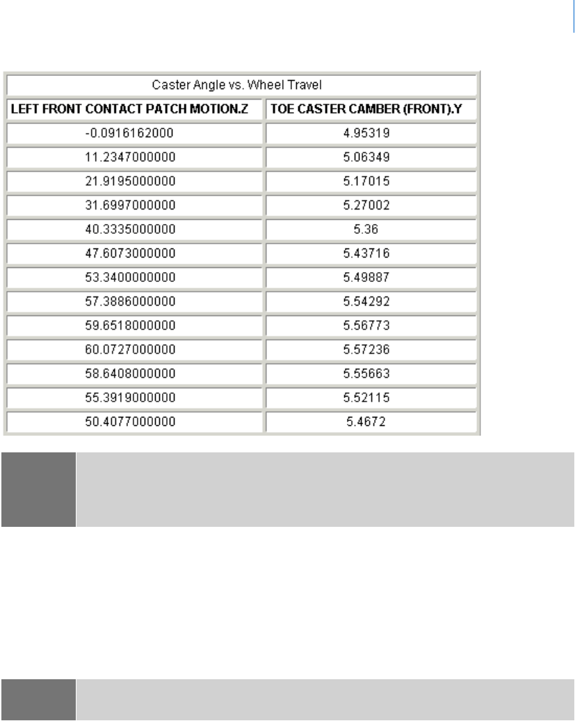
59
Building Plots
Displaying Plots as Tables
Changing a Plot to a Table
To change a plot to a table:
1. In the Treeview, select a two-dimensional plot.
2. In the
Property Editor, select Table.
Changing Table Properties
For tables, you can change the properties listed in the table below. You can also change the dependent column
(curve data) properties as explained in
Changing Dependent Column Properties.
Notes: You can still edit the data in the table in math mode as explained in Using Expressions to Modify
Curve Data Points
, although the independent data fields are not available.
You print a table as you do a plot as explained in
Printing Plots, Animations, and Reports.
Note: Even though you toggled a plot to display as a table, the treeview still lists it as a plot and all
of its columns as curves.
Adams PostProcessor
Displaying Plots as Tables
60
To change table properties:
1. Select a table.
2. In the
Property Editor, select General.
3. Set the header:
• To have Adams PostProcessor automatically generate a header, select Auto Header.
• To create your own titles and subtitles, clear the selection of Auto Header, and in the Header box,
enter the text for the header.
4. Set the general properties for the table as explained in the table below.
Curve Property Options
Column headings By default, Adams PostProcessor uses the curve legends as column headers for
the table. You can also set Adams PostProcessor to display brief headers for the
columns (for example, Column 1 instead of LEFT FRONT CONTACT
MATCH MOTION_Z) and display a legend under the header that maps
column names to data names. This is particularly helpful if you have long
column headers and need to conserve space.
Examples of Complete and Brief Headers for Tables
General appearance of
the table
You can set general properties for the table such as headers and font size. After
you set up the headers, you can change their justification and text as explained
in
Adding Notes and Modifying Text.
Display of the
independent column
You can turn off the display of the independent column and change the display
of its contents (trailing zeros, scientific notation, and so on).
Note: Even though you toggled a plot to display as a table, the treeview still lists it as a plot
and all of its columns as curves.
Note: You may want to expand the width of the Property Editor so you have more space for
entering the text. To expand the Property Editor, point to the sash on its right border.
When the cursor changes to a double-sided arrow, drag the cursor to increase the
Property Editor's size.
61
Building Plots
Displaying Plots as Tables
5. To add legend text and set the columns so they are brief, select Legend.
Adams PostProcessor adds a new row under the title containing the legend text.
6. To set the independent column properties, in the property editor, select Independent Column.
7. To remove the display of the independent column, clear the selection of On.
8. To change the legend for the independent column, enter the text in the Legend text box.
9. Set the numbering properties for the column as explained in the table below.
Independent Column Options
Changing Dependent Column Properties
You can change the way Adams PostProcessor displays the data in columns when you view a plot as a table.
You can change it for each column individually.
To change column properties:
1. Select a column (curve).
To set: Do the following:
Limits Controls which rows are displayed in the table. Specify the start and end for values in
the table (start and end are specified as values in the independent data column). Note
that these limits are the axis limits on the independent axis. When you toggle back to
a plot, they will be in effect on that axis.
Row increment Set the increment for the data to be included. For example, select 1 to include ever
data point; select 5 to include every 5th data point.
Alignment of
values in columns
Set Alignment of Values to where you want to position the values in the columns.
Size of the text In the Font Size text box, enter a font size. The font type is always Helvetica.
To set: Do the following:
Trai l i n g z e r o s Select Trailing Zeros to have Adams PostProcessor display zeros after the numbers
in the table. The number of zeros depends on the number of decimal places you
selected as explained next.
Decimal places In the Decimal Places text box, enter the number of decimal places to which the
numbers in the table should be displayed.
Scientific range In the Scientific Range text boxes, enter the exponential form for scientific
notation.

Adams PostProcessor
Displaying Plots as Tables
62
2. Set the properties for the columns as explained in the table below.
Column Options
Examples of Complete and Brief Headers for Tables
Complete Headers
Note: Even though you toggled a plot to display as a table, the treeview still lists it as a plot
and all of its columns as curves.
To set: Do the following:
Tr a i l i n g ze r o s Select Trailing Zeros to have Adams PostProcessor display zeros after the numbers
in the table. The number of zeros depends on the number of decimal places you
selected as explained next.
Decimal places In the Decimal Places text box, enter the number of decimal places to which the
numbers in the table should be displayed.
Scientific range In the Scientific Range text boxes, enter the exponential form for scientific
notation.
Caster Angle vs. Wheel Travel
LEFT FRONT CONTACT MATCH
MOTION_Z
TOE CASTER CAMBER (FRONT) Y
-0.0916152000 4.95319
11.2347000000 5.06349
21.9194000000 5.17015
31.6997000000 5.27002
40.3335000000 5.36
47.6073000000 5.43716
63
Building Plots
Automatically Re-Generating Plots
Brief Headers
Automatically Re-Generating Plots
To automatically recreate a set of interactively-built plots in the future for the same or different analyses one
can use the
Plot Configuration Files.
Caster Angle vs. Wheel Travel
Column 1: LEFT FRONT CONTACT
Column 2: TOE CASTER CAMBER
Column 1 Column 2
-0.0916152000 4.95319
11.2347000000 5.06349
21.9194000000 5.17015
31.6997000000 5.27002
40.3335000000 5.36
47.6073000000 5.43716

Adams PostProcessor
Automatically Re-Generating Plots
64
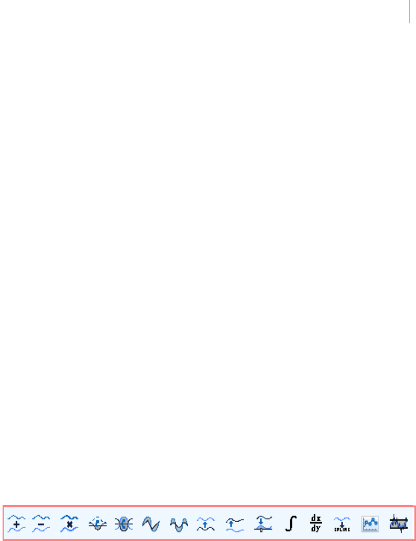
1
Manipulating Curve Data
Performing Calculations on Curves
Manipulating Curve Data
Performing Calculations on Curves
Adams PostProcessor provides you with several tools to help you perform post-processing operations on data
in plots. You can perform mathematical calculations on the data in any curve, including:
Add, subtract, or multiply values in a curve by values in another curve.
Find the absolute value of curve values or negate the values.
Interpolate the values in a curve to create an evenly spaced sampling of the curve values.
Scale a curve by a specified value.
Offset a curve by a specified value. Offsetting a curve shifts the data along the corresponding axis.
Align one curve to the starting point of another curve or align a curve so it starts at zero. Aligning
one curve to another can help you compare the data in the curves.
Differentiate the data in one curve over the closed interval represented by a second curve or define
an integral.
Create a spline from the curve values.
Manually change the values in the curve.
Filter the curve data.
You can create a new curve based on the calculations or modify the first curve that you select for an operation.
Learn more about performing calculations on curves:
Displaying the Curve Edit Toolbar
Performing Simple Mathematical Calculations on Curve Data
Calculating Integral or Differential of Curve Data
Creating Splines from Curves
Manually Changing Data Point Values
Using Expressions to Modify Curve Data Points
Displaying the Curve Edit Toolbar
When you choose to perform mathematical calculations, Adams PostProcessor displays a Curve Edit toolbar,
as shown below.
To toggle on and off the display of the Curve Edit toolbar:
On the View menu, point to Toolbars, and then select Curve Edit Tool Bar.
Adams PostProcessor
Performing Calculations on Curves
2
The Curve Edit toolbar appears at the top of the window below the Main toolbar.
Performing Simple Mathematical Calculations on Curve Data
You can modify the values in a curve by performing simple mathematical calculations on the values. You can
use the values contained in another curve or specify a value. The curves on which you perform the operations
must belong to the same plot.
To perform mathematical calculations on curves:
1. If you want to modify a curve based on the values and not create a new curve, at the far right of the
Curve Edit toolbar, clear the selection of Create New Curve. Adams PostProcessor modifies the first
curve for those operations requiring two curves (for example, subtraction).
2. Select a tool from the Curve Edit toolbar and enter any requested values as explained in the table
below.
Simple Mathematical Calculations
Tip: From the Main toobar, select .
Note: The Curve Edit toolbar automatically detects when curves are incompatible, and either clips
or fits an Akima spline to the curves to assist in performing curve math.
To: Do the following:
Add, subtract, or
multiply values in a
curve by values in
another curve
1. Select one of the following tools from the Curve Edit toolbar depending on
the operation that you want to perform:
• Add Curve Data tool .
• Subtract Curve Data tool .
• Multiply Curve Data tool .
2. Select the curve that you want values to be added to, subtracted from, or
multiplied by.
3. Select the second curve.
Find the absolute
values of data points
or negate data points
1. From the Curve Edit toolbar, select one of the following tools depending
on the operation you want to perform:
• Absolute Value tool .
• Negate tool .
2. Select a curve.
3
Manipulating Curve Data
Performing Calculations on Curves
Calculating Integral or Differential of Curve Data
You can calculate the definite integral or differential function of existing data points. The definite integral
operation evaluates the area under the data curve over the closed interval represented by the curve data.
Create evenly spaced
sampling of curve
values (interpolate
values)
1. From the Curve Edit toolbar, select the Curve Sampling tool .
2. From the pull-down menu on the right of the toolbar, select the spline type
to be used for the interpolation.
• akima - Uses the Akima method as documented in Journal of the
Association Computing Machinery, Volume 17, No 4, October 1970.
• linear - Uses the first order LaGrangian interpolation.
• cubic - Uses the second order LaGrangian interpolation.
• cspline - Performs a global fit.
• notaknot - Interpolates using the Not-a-knot cubic spline.
• hermite - Interpolates using the Hermite cubic spline.
3. Enter the number of interpolation points to be used to fit the data. The
default is 1024. You must enter a positive integer. If you are preparing the
curve for an FFT operation, we recommend that the number of points be
an even power of two (for example, 256, 512, 1024, and so on).
4. Select a curve.
Scale or offset a
curve by a specified
value
1. From the Curve Edit toolbar, select one of the following tools depending
on the operation you want to perform:
• Scale tool .
• Offset tool .
2. In the text box that appears at the far right of the Curve Edit toolbar, enter
the scale or offset value.
3. Select a curve.
Note: Select and drag the curve to a new location.
Align one curve to
the starting point of
a second curve
1. From the Curve Edit toolbar, select Align Curve to Curve tool .
2. Select a curve whose values you want to align.
3. Select a second curve.
Align a curve so it
starts at zero
1. From the Curve Edit toolbar, select Align Curve to Zero tool .
2. Select a curve.
To: Do the following:
Adams PostProcessor
Performing Calculations on Curves
4
Integral - Adams PostProcessor calculates the integral by fitting a cubic spline to the curve data and
analytically evaluating the definite integral. In other words, the cubic spline fit gives a polynomial
representation of the segments that represent the data. Adams PostProcessor then analytically
integrates the polynomial over the closed interval of the data.
Differential - Adams PostProcessor numerically differentiates the curve data over the closed interval
represented by the finite set of data points in the curve.
Adams PostProcessor evaluates the derivative by fitting a cubic spline to the curve data and
analytically forming the derivative. The cubic spline fit gives a polynomial representation of the
segments that represent the data. Adams PostProcessor then analytically differentiates the polynomial
over the closed interval of the data.
To calculate the integral or differential:
1. From the Curve Edit toolbar, select either of the following depending on the operation that you want to
perform:
• Integrate tool .
• Differential tool .
2. Select a curve on which the calculations will be performed.
3. Select a second curve.
Creating Splines from Curves
You can take the data points in a curve and create a spline from them. You can use the splines to define
motions or forces. You can also export the spline to be used as a loadcase in a finite-element program.
To use the spline that you create in your model definition, you must write a function expression that includes
Adams spline functions (such as
Akima Fitting Method (AKISPL) or Cubic Fitting Method (CUBSPL)) or create a User-
written subroutine
that calls one of the spline utility subroutines (AKISPL or CUBSPL subroutine).
For more information on using splines in:
Adams View, see Splines, in the Adams View online help.
Expressions, see the Adams View Function Builder online help.
User-written subroutines, see Welcome to Adams Solver Subroutines.
Once you have created a spline, you can modify it through Adams View. You use the Build -> Data Elements
-> Spline -> Modify command.
To create a spline from data points:
1. From the Curve Edit toolbar, select Spline tool .
2. In the Spline Name text box that appears on the left of the Curve Edit toolbar, enter the name that
you want assigned to the spline.
3. Select the curve from which you want to create the spline.
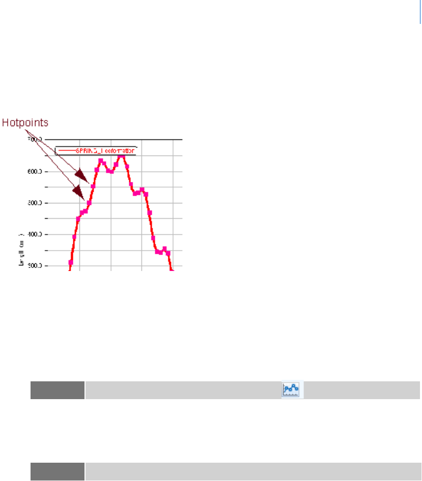
5
Manipulating Curve Data
Performing Calculations on Curves
Manually Changing Data Point Values
You can change the data point values manually for any curve you've created. When you change values
manually, Adams PostProcessor displays hotpoints at each vertex as shown below. You can control your
changes by restricting the hotpoints to only move vertically or horizontally.
To manually change data points values:
1. Select the curve on which you want to display hotpoints.
2. In the
Property Editor, set Hotpoints to:
• Yes - To move the hotpoints in any direction.
• Vertical - To move the hotpoints only vertically.
• Horizontal - To move the hotpoints only horizontally.
3. Position the cursor on a hotpoint and drag the hotpoint to the desired location.
Using Expressions to Modify Curve Data Points
You can use the Adams View Function Builder from Adams PostProcessor to create mathematical expressions
that generate curve data as output. As with any expression in Adams, an expression creating curve data can
contain basic math, trigonometric, and signal-processing functions. For more information on writing
expressions, see the
Adams View Function Builder online help.
Tip: From the Curve Edit toolbar, select Hotpoints tool .
Note: To make more precise changes, zoom in on the curve.

Adams PostProcessor
Filtering Curve Data
6
To modify a curve based on expressions:
1. Select a curve.
2. From the
Dashboard, select Math.
3. Enter the expressions for x and y data in the appropriate text boxes and define the unit values. To
display the Function Builder to help you create expressions, clear the text boxes and double-click. You
can also use the shortcut menu that appears when you right-click the text box.
4. In the Legend text box, enter the text that you want used in the legend for the curve.
5. Select OK.
Filtering Curve Data
You can filter curve data to eliminate noise on time signals or to emphasize a specific frequency content of a
time signal. Adams PostProcessor supports two different types of filters:
Butterworth filter - butter() in MATLAB developed by The MathWorks, Inc.
Transfer function - A filter you define by directly specifying the coefficients of a transfer function.
Once you create a filter, you can apply it to any curve.
Learn more about the filters and how to create and apply them:
About Filtering Methods
Creating and Modifying a Filter Function
Applying a Filter Function
Example of Creating a Filter
About Filtering Methods
Adams PostProcessor provides two filtering methods for Fast fourier transform (FFT):
Analog filtering - The numerical procedure for analog filtering is equivalent to:
• Transfer the time signal into frequency domain through FFT.
• Multiply the resulting function by the filter function.
• Perform an inverse FFT.
Digital filtering - Digital filtering operates directly on the time signal. The filtered signal at a certain
time step is a linear combination of previous input and output signals, with the discrete transfer
function defining the coefficients.
Note: Be careful with the division operation. It has problems if you divide by zero. You get errors
similar to the following:
ERROR: Division by zero
ERROR: Expression entered for vertical axis is invalid.
7
Manipulating Curve Data
Filtering Curve Data
Creating and Modifying a Filter Function
You use Filter command on the Plot menu to create or modify a filter function. You can create a Butterworth
filter or a transfer function. For the transfer function, you can define the coefficients manually or by defining
a Butterworth filter.
To create or modify a Butterworth function:
1. From the Plot menu, point to Filter, and select either Create or Modify. If you selected Modify, select
the name of the filter to modify from the Database Navigator.
The
Create/Modify Filter Function dialog box appears.
2. If you are creating a filter, in the Filter Name text box, enter the name you want to assign to the filter
function.
3. Select Butterworth Filter.
4. Set the filter type, order, and frequency of cutoff.
5. Select OK.
To create a filter based on a transfer function:
1. From the Plot menu, point to Filter, and select either Create or Modify. If you selected Modify, select
the name of the filter to modify from the Database Navigator.
The
Create/Modify Filter Function dialog box appears.
2. If you are creating a filter function, in the Filter Name text box, enter the name you want assigned to
the filter function.
3. Select Transfer function.
4. Select a
filtering method.
5. Enter the numerator and denominator coefficients as explained in the
table below. You can enter the
coefficients manually or use a Butterworth filter to define them.
6. To check the format and plot the filter's gain and phase, select Check Format and Display Plot.
Tip: Shortcut for creating a filter:
From the
Curve Edit toolbar, select the Filter Curve tool . Right-click the Filter
Name text box, point to filter_function, and then select Create.
Tip: Shortcut for creating a filter:
From the
Curve Edit toolbar, select the Filter Curve tool . Right-click the Filter
Name text box, point to filter_function, and then select Create.
Adams PostProcessor
Filtering Curve Data
8
If you have not defined the filter correctly, an error message appears. If you've defined the filter
correctly, a plot appears in which you can switch between the filter's gain and phase plots and change
scales.
7. To associate comments with the filter function, select the Comments tool , and then enter the
comments.
8. Select OK.
Options for Entering Coefficients
Applying a Filter Function
To apply the filter you created:
1. Select a curve to filter.
2. From the
Curve Edit toolbar, select the Filter Curve tool .
3. In the Filter Name text box, enter the name of the filter function.
4. To check if compensation for filter lag should be used, select Zero Phase. (Not available for
analog
filters
.)
Zero-phase digital filtering filters the input data in both forward and reverse directions. The resulting
sequence has precisely zero-phase distortion and double the filter order.
5. Select OK.
To enter the
coefficients: Do the following:
Manually Enter the numerator and denominator coefficients. See Create/Modify Filter
Function
dialog box help for more information.
Using a Butterworth
filter
1. Select Create from Butterworth Filter. See Create Butterworth Filter dialog
box help for more information.
2. Do one of the following:
To specify the order and scaled cutoff frequency values directly, enter
them at the top of the dialog box.
To generate them based on Passband and Stopband options, select the
checkbox Generate Filter Order _ Frequency. Set the values that
appear in the dialog box, and then select the Generate Order _
Frequency button.
3. Select OK.
The transfer function coefficients appear in the Create Filter Function
dialog box.

9
Manipulating Curve Data
Filtering Curve Data
Example of Defining a Transfer Function from a Butterworth Filter
The following example shows how you can define a transfer function by defining a Butterworth filter. The
Butterworth filter that you will create is a Basspand filter, based on specifying two values each for passband
and stopband corner frequency.
To define a transfer function from a Butterworth filter:
1. From the Curve Edit toolbar, select the Filter Curve tool .
2. Right-click the Filter Name text box, point to filter_function, and then select Create.
The
Create/Modify Filter Function dialog box appears.
3. In the Filter Name text box, enter bandpass_filter1.
4. Select Transfer function.
5. Select Analog.
6. Set Filter Type to Band Pass.
7. Select Create from Butterworth Filter.
8. Select the Generate Filter Order _ Frequency checkbox.
9. In the Passband Corner Frequency (WP) (Hz) text box, enter 5,8.
10. In the Stopband Corner Frequency (WS) (Hz) text box, enter 2, 10.
11. Leave the default values for Passband Ripple (3) and Stopband Attenuation (15).
12. Select Generate Order _ Frequency.
Adams PostProcessor loads the appropriate values in the Order and Cutoff Frequency text boxes at
the top of the dialog box. See the dialog box below for how the values appear.
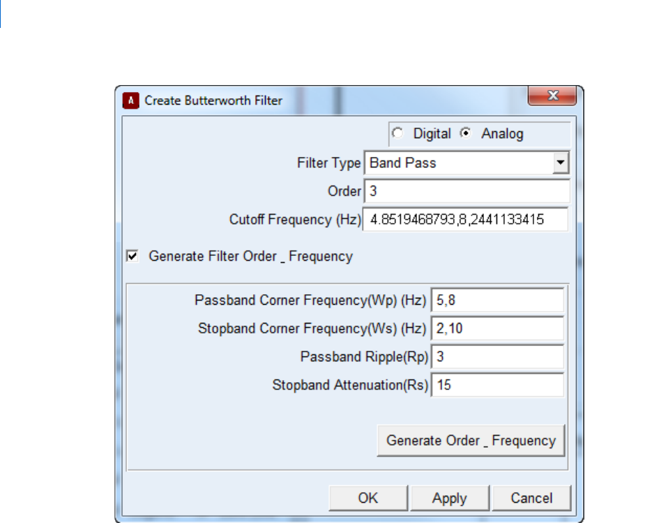
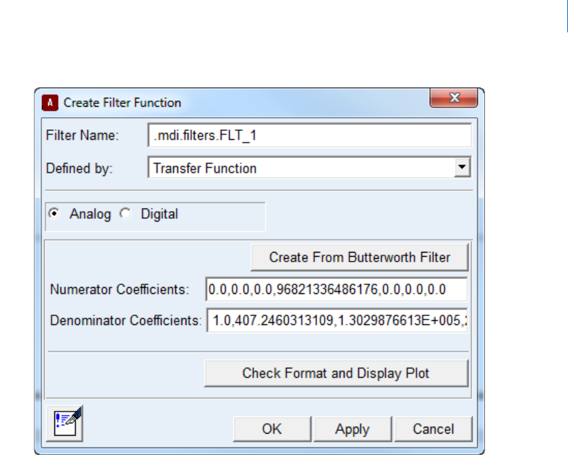
11
Manipulating Curve Data
Filtering Curve Data
2. Select Check Format and Display Plot.
3. When the plot appears, set the Min to 0.1 and then select Redraw.
The plot appears as follows:
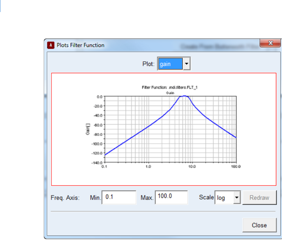
Adams PostProcessor
Performing FFT Functions
12
Notice that:
Between 5 and 8 Hz, the maximum damping is 3dB (specified by the Passband Ripple option).
At 10 Hz, the damping is 15 dB (specified by the Stopband Attenuation option).
At 2 Hz, the damping is more than 15 dB; therefore, in this case, it is not a defining factor.
Performing FFT Functions
Learn about Fast fourier transform (FFT) options, how to perform an FFT on a curve, and how to construct a
three-dimensional plot.
FFT Representations
Window Types
Constructing a Two-Dimensional FFT Plot
Constructing a Three-Dimensional FFT Plot

13
Manipulating Curve Data
Performing FFT Functions
FFT Representations
Adams PostProcessor contains three methods of representing frequency-domain data:
FFTMAG
FFTPHASE
PSD (Power Spectral Density)
FFTMAG
FFTMAG (FFT magnitude) determines the magnitude (abs) of the complex value returned from the FFT
algorithm. Adams PostProcessor only plots the left spectrum of the frequency data with the frequency on the
independent, x-axis, and the magnitude on the dependent, y-axis. The right half of the spectrum is a mirror
image of the left half.
Adams PostProcessor scales FFTMAG data by 1/(N/2) where
N is the number of time-domain samples. This
provides the effect of representing the FFTMAG peak in the magnitude of the time-domain data. The
following is an example:
The FFTMAG plot has a peak of 2 at 1 Hz and a peak of 8 at 12 Hz.
FFTPHASE
FFTPHASE determines the phase angle of the complex value returned from the standard FFT algorithm.
FFTPHASE, at a given frequency, indicates the phase shift of the equivalent sine function represented in the
time-domain data. The phase shift of a sinusoidal is phi in the following expression:
PSD (Power Spectral Density)
The signal of any time-dependent model has the same total power in the time domain as in the frequency
domain. What is of interest in spectral analysis is the amount of power contained over a frequency interval.
A PSD plot represents the distribution of power of a signal among its frequency components. In general, a
PSD plot looks like a FFTMAG plot, but on a different scale.
Adams PostProcessor creates a one-sided power spectral density. Therefore, the scaling it uses is:
Ft() 22πt()82π12t()sin+sin=
Notes: FFTMAG is extremely useful for determining the natural frequencies of structures.
On the FFT dialog box, there is an option, Detrend Input Data. It removes DC shifts in
the data over time. Adams PostProcessor fits a linear regression to the data and subtracts it
from the data before performing an FFT.
ft() Ct φ+()sin=
PH f() fft f()
2
fft f–()
2
+=

Adams PostProcessor
Performing FFT Functions
14
The PSD option on the FFT dialog box uses the pwelch function in Matlab. The sum of PSD, as computed
by pwelch, is equal to the time-integral squared amplitude of the original signal. The pwelch function
calculates the PSD using Welch's method:
The input signal vector x is divided into k overlapping segments according to window and noverlap
(or their default values).
The specified (or default) window is applied to each segment of x.
An nfft-point FFT is applied to the windowed data.
The (modified) periodogram of each windowed segment is computed.
The set of modified periodograms is averaged to form the spectrum estimate S(e
j
).
The resulting spectrum estimate is scaled to compute the power spectral density as S(e
j
)/F, where
F is:
• 2 pi when you do not supply the sampling frequency.
• fs when you supply the sampling frequency (we use this option in Adams).
The number of segments k that x is divided into is calculated as:
Eight if you do not specify the window, or if you specify it as the empty vector [].
k= (m-o)/(l-o) if you specify window as a nonempty vector or a scalar.
In this equation, m is the length of the signal vector x, o is the number of overlapping samples
(noverlap), and l is the length of each segment (the window length).
Window Types
The FFT algorithm assumes that the time-domain data is a periodic sample from a continuous, infinite series
of data. The beginning and end conditions are, therefore, assumed to match. Window functions are filters
that reduce discontinuities from mismatching start and end conditions and ensure periodicity of the FFT.
The window functions are listed below with the equation used to define the window. In the equation,
Wj is
the window function and
N is the number of input samples.
Window functions that closely resemble the unit step input retain the magnitude of the FFT output, but
accept minimal discontinuities before the FFT integrity is lost. Likewise, window functions that tend to
decrease the accuracy of the peak frequency magnitudes, significantly reduce the negative impact of end
condition discontinuities. The application of different window functions depends on the situation and your
preference.
Note: In general, the rectangular window function represents the ideal magnitudes most accurately,
but are the most sensitive to discontinuity. The Hanning window function filters the largest
discontinuities but represents the ideal magnitudes with the least accuracy.
15
Manipulating Curve Data
Performing FFT Functions
Window
Functions
Equation Used to Define the Window
Rectangular
Hanning
Hamming:
Welch
Parzen
W
j
1
2
---
1
2πj
N 1–
-------------
cos–=
W
j
0.54 46
2πj
N
--------
cos–=
W
j
1
j
1
2
---
N 1–()–
1
2
---
N 1+()
-----------------------------
–=
W
j
1
j
1
2
---
N 1–()–
1
2
---
N 1+()
-----------------------------
–=

Adams PostProcessor
Performing FFT Functions
16
Bartlett For n odd:
For
n even:
Blackman
Tr i a n g u l a r For n odd:
For
n even:
Window
Functions Equation Used to Define the Window
wj[]
2 j 1–()
n 1–
------------------
, 1 j
n 1+
2
------------
≤≤
2
2 j 1–()
n 1–
------------------
,–
n 1+
2
------------
jn≤≤
=
wj[]
2 j 1–()
n 1–
------------------
, 1 j
n
2
---
≤≤
2
2 j 1–()
n 1–
------------------
,–
n
2
---
1+ jn≤≤
=
wj[] 0.42 0.5 2π
j 1–
n 1–
------------
0.08 4π
j 1–
n 1–
------------
cos+
·
j,cos– 1 ...,n,==
wj[]
2j
n 1+
------------
, 1 j
n 1+
2
------------
≤≤
2
2 nj–1+()
n 1–
----------------------------
,–
n 1+
2
------------
jn≤≤
=
wj[]
2j
n 1+
------------
, 1 j
n
2
---
≤≤
2
2 nj–1+()
n 1–
----------------------------
,–
n
2
---
1+ jn≤≤
=

17
Manipulating Curve Data
Performing FFT Functions
Constructing a Two-Dimensional FFT Plot
To create an FFT plot:
1. Select the one or multiple curves on which you want to perform the signal processing.
2. From the Plot menu, select FFT.
The
Fast Fourier Transform (FFT) dialog box appears.
3. Select/Browse one or multiple source curves in "Curve Name" field.
4. Set y-axis to Mag, Phase, or PSD.
5. Enter the start and end time on the curve between which you want the signal processing performed.
6. Select the type of window function you want to use.
Learn about window types.
7. Specify the number of interpolation points used in fitting the data. The number of points must be a
positive integer.
8. Select Add Curves to plot multiple curves on same FFT plot window. Continuous pressing of "Add
Curves" will superimpose more FFT curves on the same plot.
9. To clear the FFT plot window, select Clear Plot button.
Constructing a Three-Dimensional FFT Plot
You can construct a three-dimensional (3D) Fast fourier transform (FFT) plot by performing signal processing on
individual slices of a curve. You define a slice size, and Adams PostProcessor slides this over a range of the
curve, overlapping the slices as specified. Each slice of the curve becomes a row in the 3D plot surface.
To create a 3D FFT plot:
1. Select the curve on which you want to perform the signal processing.
2. From the Plot menu, select FFT 3D.
The
Fast Fourier Transform (FFT) 3D dialog box appears.
3. Select the type of data to plot in the y-axis: Mag, Phase, or PSD.
4. Enter the start and end time to define the entire range of the curve on which you want signal
processing performed.
Note: When you specify the number of points, you are specifying the number of
interpolation points used to fit the data in a result set component. Earlier FFT
methods required the number of points to be an even power of two (for example,
256, 512, 1024, and so on). With new methods, however, this is no longer necessary.
You can select any number of points and the FFT method uses approximation
methods to calculate the results. We continue to recommend, however, that the
number of points be an even power of two because the results are more precise and
the FFT creation is faster.

Adams PostProcessor
Constructing Bode Plots
18
5. In Time Slice Size, enter the width of the slice on which to perform signal processing, and in
Percentage Overlap, enter the percentange amount the slices can overlap.
6. Select the type of
window function you want to use.
7. Specify the number of interpolation points used in fitting the data. The number of points must be a
positive integer.
8. Select Apply.
Tips on Selecting Points
When you specify the number of points, you are specifying the number of interpolation points used to fit the
data in a
Result set component. Earlier Fast fourier transform (FFT) methods required the number of points to be an
even power of two (for example, 256, 512, 1024, and so on). With new methods, however, this is no longer
necessary. You can select any number of points and the FFT method uses approximation methods to calculate
the results. We continue to recommend, however, that the number of points be an even power of two because
the results are more precise and the FFT creation is faster.
Notes on FFT 3D Plotting
X values must be in strictly ascending order.
Frequency option only works with evenly spaced input points. Use interpolate on the curve math toolbar
with even output steps turned on to get evenly spaced points.
Constructing Bode Plots
Bode plots provide a way to study frequency response functions (FRFs) for linear systems and linearized
representations of nonlinear systems. The frequency response function measures the response at the outputs
due to unit harmonic excitation at the inputs at various frequencies. A Bode plot in Adams PostProcessor
shows the amplitude gain and the phase shift between input to output for all output/input combinations of
the linear system.
Ways to Construct Bode Plots
Creating a Bode Plot
Bode Plot Tutorial
Note: When you simulate a model to create results you are going to view as a Bode plot, specify the
number of output steps as a power of two minus one. By specifying an even power minus
one, the number of data points in the results is a power of two (the output steps you
requested plus one for the model's initial condition). While this is not required, we
recommend you do so to obtain peak performance on Bode calculations. Learn more about
Simulation Basics in Adams View.

19
Manipulating Curve Data
Constructing Bode Plots
Ways to Construct Bode Plots
Adams PostProcessor offers seven variations of what are, essentially, three separate ways to construct Bode
plots, depending on how the linear system is represented. These are:
Transfer Functions
Linear State Space Matrices and ABCD Matrices
Input/Output Signal Pairs
Transfer Functions
A transfer function is a ratio of two polynomials in the Laplace domain when used with associated array data
elements as shown below:
Adams PostProcessor has methods that you can use to generate a Bode plot from a transfer function:
TFSISO (Adams transfer function, single-input, single-output) - TFSISO is an Adams transfer
function element.
Transfer Function Coefficients - A transfer function is a ratio of the input to the output of a system.
Adams PostProcessor converts the numerator and denominator of a transfer function from a time
domain to a Laplace domain. A Laplace domain takes integrals and derivatives and replaces them
with polynomials. Therefore, a system’s input and output can be modeled by the coefficients of the
numerator and denominator polynomials.
Linear State Space Matrices and ABCD Matrices
Another common way of representing a linear system is through a state-space representation or ABCD
matrices:
where u, y, and x denote input, output, and internal states, respectively.
The Adams PostProcessor Bode plot functionality has three ABCD matrix modes:
Adams matrices - Direct user input of Adams PostProcessor matrix elements.
Adams linear state matrix - Linear state matrices generated through a linearization of an Adams
model using Adams Linear, an optional module to Adams.
Ts()
b
0
b
1
s
1
...+b
n 1–
s
n 1–
b
n
s
n
++ +
a
0
a
1
s
1
...+a
n 1–
s
n 1–
a
n
s
n
++ +
------------------------------------------------------------------------------
=
x
·
Ax Bu
y
+
Cx Du+
=
=
Note: You must precede a linear simulation with a linear static or dynamic simulation
because you need to establish an operating point for the linearization. Before
computing the Adams linear state matrix, you must define plant inputs and outputs,
otherwise, Adams PostProcessor sets the B, C, and D matrices to zero.

Adams PostProcessor
Constructing Bode Plots
20
Linear State Equation - ABCD matrices encapsulated in an Adams linear state equation system
element.
Input/Output Signal Pairs
You can generate a Bode plot using two sample time signals for the input and output channels. Adams
PostProcessor estimates the frequency response function by performing a Fast Fourier Transform of the two
signals and computing a complex ratio of the two frequency domain series. The gain and the phase shift in
the Bode plot are the real and imaginary parts of this ratio. Adams PostProcessor allows the Bode plot to be
generated by representing the input signal using result set component or Adams PostProcessor measures.
Time domain results set components (RSC) - The RSC method uses output from a simulation to
define the system.
Time domain measures - The time domain measure method uses predefined or user-defined
measures of model input and output to define the system.
Creating a Bode Plot
To create a bode plot:
1. From the Plot menu, select Bode Plots.
The
Bode Plots dialog box appears.
2. Select the type of input format. For more information, see
Ways to Construct Bode Plots.
The elements in the dialog box change depending on the input format that you selected.
3. Enter the values in the dialog box as explained in the
Bode Plots dialog box help, depending on the
input format, and then select OK.
1
Viewing Reports
Viewing Reports
In this section you will Learn more about importing and viewing Reports.
Exporting Adams PostProcessor Data as an HTML Report
You can export the following Adams PostProcessor data in the current session of Adams PostProcessor as an
HTML
report for viewing by others in your organization:
Information on the parts, constraints, forces, and more in the selected models. This is the same
information that appears when you select Info.
Plots and animations as .png or .jpg images.
Movies of animations.
The result is a series of HTML pages, images, and style sheets, including a main homepage. See Export -
HTML Report for more information.
To export data as an HTML report:
1. From the File menu, point to Export, and then select HTML Report.
The Export Dialog Box appears.
2. Under the Files tab, enter the name you want applied to each of the resulting HTML files and style
sheets, and enter where you want the resulting HTML files and folders to be stored.
3. Under the Title Page tab, enter the title, author, date, and any comments you want displayed on the
title page. The title page appears when you first display the homepage. You can also enter an image
to appear in the upper right corner of the title page. The image can be of any format that you can
display in a Web browser (such as .gif, .jpg, .png).
4. Under the Pages tab, enter the following:
Options for Pages Tab
To: Do the following:
Pages Select the pages of plots and animations you want exported. If you select Range,
enter the pages you want included.
Image Format Enter the image format in which to store the pages of plots. You can select png or
jpg.
Image Width and
Height
Enter the pixel size of the exported pages. By default, Adams PostProcessor
maintains the aspect ratio of the images so if you enter a value for width, Adams
PostProcessor automatically calculates the height based on the current aspect
ratio, and the reverse. See Maintain Aspect Ratio below.
If you leave both text boxes blank, Adams PostProcessor uses their default size in
Adams PostProcessor.
Adams PostProcessor
2
5. Under the Models tab, select the models for which you want to export information about their
objects.
6. Select OK.
Adams PostProcessor begins creating the exported data. If you selected to export an animation, you
see the animation being recorded.
To display the results of the export:
1. In a Web browser, change to the folder containing the results of the export.
2. Select the file with the same name as that you entered in the Files tab. For example, if you entered
suspension_1, select suspension_1.htm.
Loading Reports
You can load simple HTML and ASCII reports into Adams PostProcessor.
To import a report:
1. From the File menu, point to Import, and then select Report.
2. Enter the name of the file to import.
3. Select OK.
To load a report in a viewport:
Right-click the background of a viewport, and then select Load Report.
Maintain Aspect Ratio Clear to change the proportions of the page sizes, and then enter new values for
Image Width and Height (see above).
Export Animations Select to export the animations as a movie. Clear to just save an image of the first
frame of the animation in the same format selected in Image Format.
Movie Format Select the type of movie to export the animation as. You can select: Compressed
.avi, Uncompressed .avi, .jpg, .mpg, and .png (AVI format is only available on
Windows).
If you select .jpg or .png, Adams Processor, exports each frame as an png
or jpg file, and then plays them as a movie.
If you select compressed AVI format, set the frame rate, interval between
key frames, and quality (percentage of compression). The default is 75%
compression with each key frame 500 frames apart, and a frame rate of
10 seconds per frame.
If you select .mpg, set options to be able to play the movie in many
playback programs. For more on these options, see
Recording Animations.
To: Do the following:
3
Viewing Reports
Modifying Report Properties
After you import a reports, you can change the source file associated with the report and the font point size
associated with the HTML logical font point size 3 (HTML logical font point sizes are from 1 to 7; they
define font point sizes relative to one another; not in absolute values). All other font point sizes are scaled
accordingly. For example, if you set the report font point size to 10 points, then logical font size 3 is 10; font
size 2 is 8 points; and so on.
To modify report properties:
1. Select a report.
2. In the
Property Editor, in the File Name text box, change the source file for report.
3. In the Font Size text box, enter the size for logical font size 3.
Updating Reports
You can update reports just as you update the results of simulations using the Recycle button and
Replace Simulations command. They check the dates of the report files on disk and reload them if the file
date has changed. Learn about Updating Plot Data.
HTML Tags Supported in Reports
Adams PostProcessor supports only a subset of all HTML tags and does not support links. The following
tables show the HTML tags that Adams PostProcessor supports:
Structuring Tags Supported
Character Tags Supported
Special Tags Supported
Table Tags Supported
Structuring Tags Supported
The tag: Represents:
<h1>...</h1>
Top-level heading.
<h2>...</h2>
Sub-level heading.
<h3>...</h3>
Sub-sub-level heading.
<p>...</p>
Left-aligned paragraph. Adjust the alignment with the align
attribute. Possible values are left, right and center.
<center>...</center>
Centered paragraph.
<blockquote>...</blockquote>
Indented paragraph.
Adams PostProcessor
4
Character Tags Supported
Special Tags Supported
<ul>...</ul>
Unordered list.
<ol>...</ol>
Ordered list. You can also define the enumeration label using
the type attribute. The default is type="1"; other types are "a"
and "A".
<li>...</li>
List item.
<pre>...</pre>
Leaves the information as is with no formatting. Preserves white
spaces in the content.
The tag: Represents:
<em>...</em>
Emphasized.
<strong>...</strong>
Strong.
<i>...</i>
Italic font style.
<b>...</b>
Bold font style.
<u>...</u>
Underlined font style.
<big>...</big>
Larger font size.
<small>...</small>
Smaller font size.
<code>...</code>
Indicates code.
<tt>...</tt>
Typewriter font style.
<font>...</font>
Information on fonts, including color, size, and type (face). The tag
understands the following attributes:
color - The text color, for example: color="#FF0000"
size - The logical size of the font. Logical sizes 1 to 7 are
supported. The value can either be absolute (for example, size=3)
or relative (size=-2).
face - The family of the font, for example: face=times
The tag: Represents:
5
Viewing Reports
Table Tags Supported
The tag: Represents:
<img>
An image. The image name is given in the source attribute, for
example: <img src="qt.xpm" /> The image tag also understands
the attributes width and height, which determine the size of the
image.
<hr>
Horizontal line.
<br>
Line break.
<nobr>...</nobr>
No break.
The tag: Represents:
<table>...</table>
A table definition. Other attributes are:
bgcolor - Background color.
width - Table width. Can be a percentage or actual number of pixels.
border - Width of the table border.
cellspacing - Additional space around the table cells.
cellpadding - Additional space around the contents of table cells.
<tr>...</tr>
A table row that can only be used within table. It has the attribute:
bgcolor - Background color.
<td>...</td>
A table data cell with the following attributes:
bgcolor - Background color.
width - Cell width. Can be a percentage or actual number of pixels.
colspan - How many columns this cell spans.
rowspan - How many rows this cell spans.
align - Alignment.
<th>...</th>
Table header cell.

Adams PostProcessor
6

1
Performing Clearance Studies
Clearance Studies
Performing Clearance Studies
Clearance Studies
You can perform a clearance study that reports the minimum distance between objects in your model at each
frame of an animation. For example, you might want to perform a clearance study to ensure packaging
requirements are satisfied.
When you view an animation of the clearance study, Adams PostProcessor displays a line between the two
objects in the study to track the minimum distance. You can also plot the data and generate reports. For an
example of a clearance study, refer to the tutorial in
Getting Started Using Adams PostProcessor.
Defining a Clearance Study
To define a Clearance study:
Select the pair of objects on which you want Adams PostProcessor to report distance information
- You select objects, either parts or geometry, to be used in the study. The bodies can be rigid or
flexible. You can define many clearance objects at once by selecting multiple objects in the lists.
Set maximum distance reported - To reduce the calculations in the clearance study, you can also
define a maximum distance above which Adams PostProcessor does not calculate any distance
information. When you play an animation, if the distance between the pair of objects is greater than
the maximum distance, Adams PostProcessor does not display a line between the objects. In
addition, in clearance study reports, if the distance is exceeded at a given frame, Adams
PostProcessor records the distance as the maximum distance and not the actual distance.
Set method used for calculations - Adams PostProcessor uses two different calculations for clearance
studies:
Polygon and Vertex.
To create a clearance study:
1. From the Tools menu, point to Clearance, and then select Create.
The Create Clearance Study dialog box appears.
2. Set up the pairs to be investigated in the study.
• In the Model list, select the model to be used for the study.
• In the I Body list, select the first object in the pair. You can also select Pick to select the object
from the screen. (You can select more than one object at a time.)
• In the J Body list, select the second object in the pair. You can also select Pick to select the object
from the screen. (You can select more than one object at a time.)
3. Enter a name for the study. If you are creating several studies (by selecting more than one pair of I
and J Bodies), you can enter a base name for the studies, and Adams PostProcessor will add a suffix
to the name (base_1, base_2, and so on).

Adams PostProcessor
Clearance Studies
2
4. Set the maximum distance for the clearance beyond which clearances will not be computed at any
given frame. For more information, see the overview on the previous page. Leave the text box empty
if you always want to calculate the minimum distance.
5. Select the method for calculating the minimum distances, either:
Polygon or Vertex
6. Select OK.
7. Run clearance study as explained in
Running a Clearance Study.
Running a Clearance Study
When you request to run a Clearance study, Adams PostProcessor calculates the minimum and
maximum distances between a pair of objects using data from a selected Simulation. It adds the
information to the animation associated with the simulation, which you can subsequently run. You can also
generate a report of the data and plot it.
To run a clearance study:
1. Set up the clearance study as explained in Defining a Clearance Study.
2. From the Tools menu, point to Clearance, and then select Compute.
The Clearance Compute dialog box appears.
3. Select the simulation data against which you want to run the clearance study.
4. From the pull-down menu, select if you want to calculate the clearance study as if flexible bodies were
rigid. This reduces computations and allows the clearance study to run faster but does not give you
information about the effects of flexibility.
5. Select OK.
Playing an Animation of the Clearance Study
You can review an animation of the Clearance study. When you run the animation, Adams PostProcessor
displays a line representing the minimum distance at each frame between the objects in the clearance study.
No line appears between objects if the distance between the objects is greater than the maximum value you
set, above which Adams PostProcessor performs no calculations. For more information, see
Defining a Clearance
Study
.
You can change the color of the minimum distance line, its visibility, and width.
Learn how to change the
clearance study
.
Tip: The number of frames in your animation can have a significant effect on the accuracy of the
distances reported. Therefore, for best results, we recommend that you perform at least one
clearance study with a large number of frames in the animation (time steps in the
simulation).
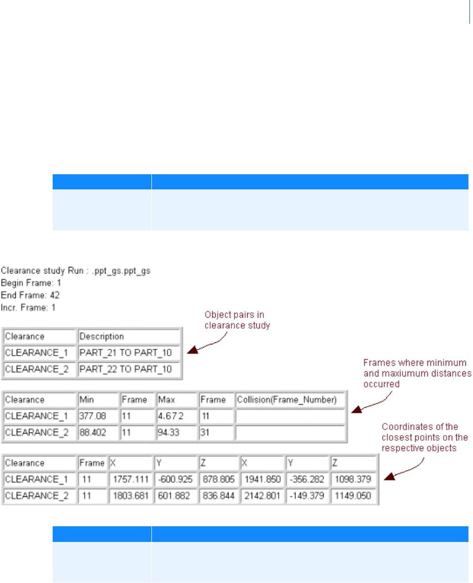
3
Performing Clearance Studies
Clearance Studies
To review a clearance study as an animation:
1. In the Treeview, under the model and Simulation on which you selected to perform the clearance
study, select the name of the clearance study.
2.
Play the animation.
Viewing Clearance Data as Reports
You can export summaries of all clearance studies run for a particular Simulation in different formats:
Example:
The format: Does the following:
Complete report in
HTML or text format
Displays the objects in the studies, frame at which minimum and maximum
distances occurred, and position of objects at minimum distances. The text file
has a .clt extension.
The format: Does the following:
Report of minimum
distances at each frame
in text format
Displays minimum distances at each frame. Has a .clr extension.

Adams PostProcessor
Clearance Studies
4
Example:
Clearance study : CLEARANCE_1
Analysis name : ppt_gs
Min 377.083 at frame 11
Max 476.712 at frame 31
Frame Distance
---------------------------
1 420.791
2 420.791
3 412.919
4 405.346
...
Clearance study : CLEARANCE_2
Analysis name : ppt_gs
Min 881.402 at frame 11
Max 940.895 at frame 31
Frame Distance
---------------------------
1 912.850
2 912.850
3 907.660
4 902.446
...
To export reports:
1. From the Tools menu, point to Clearance, and then select Write.
The Clearance Export Results dialog box appears.
2. Enter the name of the file and the simulation result against which you created the clearance studies.
3. Select OK.
For more on working with reports in Adams PostProcessor, see
Viewing Reports.
Plotting Clearance Data
After you run a Clearance study, you can plot the following information:
X, Y, and Z location of objects (I Body and J Body) in study
Minimum distance
You plot clearance study data much like you plot any data in Adams PostProcessor. For more information on
plotting, see
Plotting Results.
To plot clearance study results:
1. From the Dashboard, select the simulation on which you performed the clearance study.
2. Set Source to Clearances.
The dashboard changes to show the clearance data available for plotting.

5
Performing Clearance Studies
Clearance Studies
3. From the Request list, select the clearance study whose data you want to plot.
4. From the Component list, select one or more components of the characteristic that you want to plot.
5. Select Add Curves to add the data curve to the current plot.
Changing the Clearance Study
You can use the Property Editor to change many of the aspects of the Clearance study and run it again.
To change the clearance study properties:
1. In the Treeview, under the model and Simulation on which you selected to perform the clearance
study, select the name of the clearance study.
2. In the property editor, change the following:
• Visibility - To set the display of the minimum distance line, set Visibility to:
On - Turns on the display of the line during animations.
Off - Turns off the display of the line during animations.
• Inherit - Lets the line simply inherit the display settings from its parent.
• Line weight - Select a line weight for the minimum distance line. The weight values range from
1 to 5 screen pixels.
• Color - Set Color to the color for the minimum distance line.
• Method - Change the method used to calculate the distances: either Polygon or Vertex.
• Maximum - Set the maximum value beyond which Adams PostProcessor does not calculate. For
more information, see
Defining a Clearance Study.
3. If you changed the method or the maximum value, run the study again as explained in
Running a
Clearance Study
.

Adams PostProcessor
Clearance Studies
6

1
Setting Preferences
Saving Your Preferences
Setting Preferences
Saving Your Preferences
You can use the Preferences dialog box to easily change the ways in which Adams PostProcessor works. In
addition, you can specify the directory to which Adams PostProcessor saves files.
You can store preferences you set for use in later sessions. If you are using Adams PostProcessor stand-alone,
it stores the preferences in the file pptBS.cmd in your working directory. If you are using Adams PostProcessor
with Adams View, it stores the preferences in the file aviewBS.cmd. The BS stands for Before Startup, meaning
that Adams PostProcessor will read it before it reads any other setup files.
If Adams PostProcessor finds either pptBS.cmd or aviewBS.cmd in the current working directory or the home
directory, it automatically loads it when it starts up. Since Adams PostProcessor overwrites the file when you
save it during a session, you should not edit it manually.
To save a preferences file:
1. From the Edit menu, select Preferences.
2. Make changes as explained in the other Help topics on preferences.
3. Select Save.
You can also restore the default settings after making changes:
1. From the Edit menu, select Preferences.
2. Select Restore.
PPT Preferences
Edit -> Preferences
Changes the ways in which Adams PostProcessor works. In addition, you can specify the directory to which
Adams PostProcessor saves files.
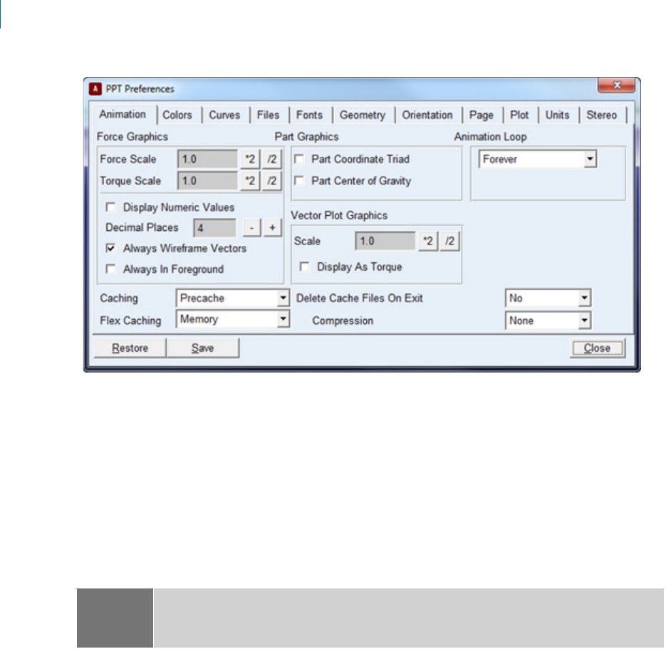
Adams PostProcessor
PPT Preferences
2
PPT Preferences - Animation
Edit -> Preferences-> Animation Tab
You can set preferences for animations, including preferences for force graphics, caching of animations, part
graphics, and flexible body display.
Learn more:
About Force Graphics
About Part Graphics
Note: For flexible bodies, you can also use the Performance Tuning Guide, which steps you through
all the preferences you can set for improving the performance of animations of flexible
bodies, including some that are on this tab. See
Tuning the Performance of Flexible Body Animations
3
Setting Preferences
PPT Preferences
For the option: Do the following:
Force graphic options:
Force Scale/Torque
Scale
Enter the amount by which you want to scale force (straight arrows) and torque
(semi-circular arrows) graphics. The default scale is 1.0 for both forces and torques.
Display Numeric
Values
Clear if you do not want to see the values of the force and torque magnitudes during
animation.
If you leave it selected, Adams PostProcessor continuously displays the magnitudes
for all force and torque graphics during the animation.
Decimal Places Enter the number of decimal places to be written for force graphics numeric values.
The default value is four.
Always Wireframe
Vectors
Clear if you want to see the force and torque graphic arrows represented as three-
dimensional objects instead of as simple lines and arcs when animating in shaded
model.
If you leave it selected, Adams PostProcessor shows the force graphics in wireframe
render mode even when you are rendering the view in shaded mode.
Always in
Foreground
Select if you want to see the graphic arrows in front of the shaded model.
Caching Set to the type of caching you want. See Caching of Animations.
Flex Caching By default, cache information necessary for animations containing flexible bodies is
maintained on disk in files with a .fcf extension. Adams PostProcessor can also
maintain this information in physical memory, which can result in significantly less
disk input/output, higher CPU utilization, and, consequently, faster performance.
If you work in an environment with remote disk servers (accessed across a network),
you should see a dramatic improvement in performance if you select to maintain the
cache in memory. Users using local disk will see improvements on a smaller scale.
The disadvantage of memory caching is the increased process size and the risk that
it will exceed your computer's physical memory. If your computer has enough
physical memory, then this approach is more efficient. If your computer doesn't have
enough physical memory, then its operating system will begin swapping and the
animation performance may be worse than when using the .fcf file. We recommend
that you test each model with this setting and monitor the process size using the Task
Manager on Windows or the equivalent tool on Linux (for example, gmemusage -s
on SGI).
Adams PostProcessor
PPT Preferences
4
PPT Preferences - Colors
Review -> Postprocessing -> Edit -> Preferences -> Colors Tab
You can change the definition of existing colors and create new colors. You can also set the color of the Adams
PostProcessor background.
Compression Three different levels of data compression are available for controlling the size of
flexible body animation caches. The levels, from the lowest to highest compression,
are None (default), Mild, and Aggressive. Each level implements a higher level of
data compression at a risk of greater data loss. Note that the compression is applied
to nodal deformations only and, therefore, may only lead to slightly incorrect
geometric representations. Contour plot information accuracy is maintained.
The disadvantage of applying data compression is that the precaching times for
certain flexible bodies may increase. Data compression should only be used when the
size of flexible body cache information needs to be minimized.
Part graphic options:
Part Coordinate
Tr i a d
Select if you want to display part coordinate triads.
Part Center of
Gravity
Select if you want to display part center of gravity markers.
Vector plot graphic options: (For more on vector plots, see Animating Flexible Bodies and Adams Durability
Results).
Scale Enter a value by which to scale the deformations. Set a large scale to exaggerate the
deformations.
Display as Torque Display vectors as linear lines or as torque vectors.
For the option: Do the following:
Color Select the color you want to modify or a color close to the color that you want to
create. If you want to change the background color, select Background.
The color appears in the color box.
New Color Select if you want to create a New Color.
Color Picker Select to create or modify a color. See Using the Color Picker to Select Colors.
For the option: Do the following:
5
Setting Preferences
PPT Preferences
PPT Preferences - Curves
Review -> Postprocessing -> Edit -> Preferences-> Curves Tab
Each time Adams PostProcessor adds a curve to an existing plot, it assigns the curve a different color and line
style so that you can differentiate between one curve and another. For example, the first curve you create is
red, the next is blue, and the third is magenta. You can change the automatic assignment of properties so that
Adams PostProcessor assigns to each curve a single color, style, and symbol that you define.
PPT Preferences - Files
Review -> Postprocessing -> Edit -> Preferences -> Files Tab
Allows you to specify how Adams PostProcessor imports Adams View command files.
Turning off the display of the commands and the results should increase the speed at which Adams
PostProcessor imports the command file.
For the option: Do the following:
Auto Color Select if you want Adams PostProcessor to automatically set the color.
If you do not select it, choose a color from the option menu.
Auto Style Select if you want Adams PostProcessor to automatically set the style of the curve.
If you do not select it, choose a style from the option menu.
Auto Symbol Select if you want Adams PostProcessor to automatically set the symbol.
If you do not select it, choose a symbol from the option menu.
Symbol Increment Select the symbol increment.
The default value of 1 specifies that a symbol is displayed on every data point on the
curve. If you have a large number of points, the symbols can obscure the curve.
Therefore, you can set higher increments to more widely distribute the symbols along
the curve. For example, if a curve has 10,000 data points, the default setting of 1
creates symbols that are too close together and obscures the curve. Setting the symbol
increment to 100 distributes only 100 symbols along the curve, making the curve
visible.
Line Weight Select the weight of the line. The weight values range from 1 to 5 screen pixels.

Adams PostProcessor
PPT Preferences
6
PPT Preferences - Fonts
Review -> Postprocessing -> Edit -> Preferences -> Fonts Tab
Allows you to specify which system fonts to use when displaying text in Viewports or when printing to
PostScript files.
For the option: Do the following:
Echo Commands Select if you want Adams PostProcessor to display the commands as it reads them
in the command window.
Update Screen Select if you want Adams PostProcessor to display the effect of each command on
the screen as it reads them or only display the final results on the screen when the
command import is complete.
On Error Select one:
Continue - Adams PostProcessor continues processing the line as if it were
typed interactively. This can be dangerous if there is no correction later on in
the line, because Adams PostProcessor keeps issuing error messages until the
error is corrected. The errors can continue beyond the end of the line, even to
the end of the file, if carriage returns are invalid. Use this value only if the
command file is a literal recording of your key strokes, complete with back
spaces or other corrections of mistakes.
Ignore - Adams PostProcessor ignores the line on which it finds the error and
starts processing the next line as a new command. Adams PostProcessor can
usually recover and execute subsequent commands in the file. If subsequent
commands depend on the results of the invalid command, however, they can
fail or give unexpected results.
Abort - Adams PostProcessor immediately stops reading the command file and
returns control to interactive input. This is the most conservative setting
because it guarantees subsequent commands will cause no further errors or
unexpected results.
Note: Changing fonts does not affect the text used to display the interface (for example, text in
dialog box or the Property Editor), reports, or tables.
7
Setting Preferences
PPT Preferences
PPT Preferences - Geometry
Review -> Postprocessing -> Edit -> Preferences -> Geometry Tab
Allows you to specify how to display and import geometry.
PPT Preferences - Orientation
Review -> Postprocessing -> Edit -> Preferences -> Orientation Tab
Allows you to change the view orientation in Viewports. By default, the view orientation of animations is set
to positive y-axis pointing up and the positive z-axis pointing out of the screen. Changing the view orientation
is particularly helpful when your models use a coordinate system that is different than the standard coordinate
system. For example, in some automotive applications, the orientation of the vehicle is such that the z-axis is
pointing up and the x-axis is pointing from the front to the rear of the vehicle. Specifying these new directions
allows the viewport orientations such as Top or Left to behave as expected with respect to the model. You can
specify any orientations as long as you do not use the same axis to define both up and forward.
For the option: Do the following:
Screen Font Enter a font type to be used for displaying text in viewports.
Postscript Font Select a font from the pull-down menu. The options available depend on the fonts
available on your computer platform.
Default Font Size Enter a size for the font.
For the option: Do the following:
Graphics Endcaps Select if you want to display endcaps. Endcaps are the ends of geometric objects,
such as cylinders and frustra. Because of the large number of edges on endcaps,
they can reduce animation performance. You can, therefore, turn off the display of
endcaps to increase the animation speed.
Trimesh geometry
during file import
Select if you want to import the triangular geometry as trimesh strips. Trimesh
strips display significantly faster than individual polygons, resulting in faster
animations. Adams PostProcessor automatically imports shell files (.shl, .slp, and
.stl) as trimesh strips. Note that when you select to import CAD files at trimesh
strips, importing of the files may be slow.
Fast transparencies Select if you want to display the transparency faster, but the quality of images
containing transparencies will suffer. By keeping this check box clear (which is the
default) better images will be displayed, especially when transparent images overlay
on each other, but at a cost of performance.
Adams PostProcessor
PPT Preferences
8
PPT Preferences - Page
Review -> Postprocessing -> Edit -> Preferences -> Page Tab
Allows you to set the header and footer that automatically appear on subsequently created pages. Each header
and footer can have three items of information (left, center, and right). Each item on the header footer can
be a bitmapped image (.jpg, .xpm, or .bmp) or text.
Set the headers and footers you want to appear on each page or select None to remove the headers and footers.
Use the Left, Center, and Right tabs to add text or images to the page header or footer.
Learn about
Managing Pages
PPT Preferences - Plot
Review -> Postprocessing -> Edit -> Preferences -> Plot Tab
Allows you to:
Specify the information that appears automatically on each plot that you create, including:
Tip: You can turn on the display of the viewport triad by selecting View in the dashboard, and
then selecting Display Triad.
For the option: Do the following:
Up Axis Select the axis to be pointing up.
Forward Axis Select the axis to be pointing out of the screen.
For the option: Do the following:
Source Choose either Text or Image.
If you set Source to Text, Adams PostProcessor displays the following options:
Text Enter the text you want to appear in the header or footer.
Font Size Enter the font size.
Color Select a color from the pull-down menu.
If you set Source to Image, Adams PostProcessor displays the following options:
Image
Enter the image you want to appear in the header or footer. The image can be a
.jpg, .xpm, or .bmp.
Height
Enter the height at which you want the image displayed. Adams PostProcessor
automatically displays the image as 50 pixels high.
9
Setting Preferences
PPT Preferences
• Titles
• Subtitles
• Analysis name and date analysis run
The information comes from the
Measures, result set, or Objects file. You can change the default as
explained in
Modifying Titles and Axis Placement.
Always display the plots as tables. (for more information, see Displaying Plots as Tables).
Set how Adams PostProcessor handles duplicate time values on curves during operations.
PPT Preferences - Units
Review -> Postprocessing -> Edit -> Preferences -> Units Tab
Allows you to set the units to be used for curve data. Adams PostProcessor scales data to the proper units
conversion factor where appropriate.
For the option: Do the following:
Auto Titles Select if you want titles to automatically appear on each plot.
Auto Subtitles Select if you want subtitles to automatically appear on each plot.
Auto Date Stamp Select if you want the date on which the simulation was performed to appear
on each plot.
Auto Analysis Name Select if you want the name of the analysis from which the plot data was
generated to appear on each plot.
Table Select if you want to always display plots as tables.
Duplicate Points Select how you want Adams PostProcessor to handle duplicate time values on a
curve. You can select:
Use last duplicate - Keeps the last value, which is the default because
the earlier time values are likely to be static steps and the last one the
dynamic step.
Use first duplicate - Keeps the first value.
Keep all duplicates - If you select to keep all duplicates, you will receive
errors messages about not being able to perform an operation because
of duplicate points. This will occur during
Curve Edit toolbar integrate
and filter operations, as well as during FFT operations.
Note: Changing the unit preferences also changes the units preferences for the complete model in
both Adams View and Adams PostProcessor.
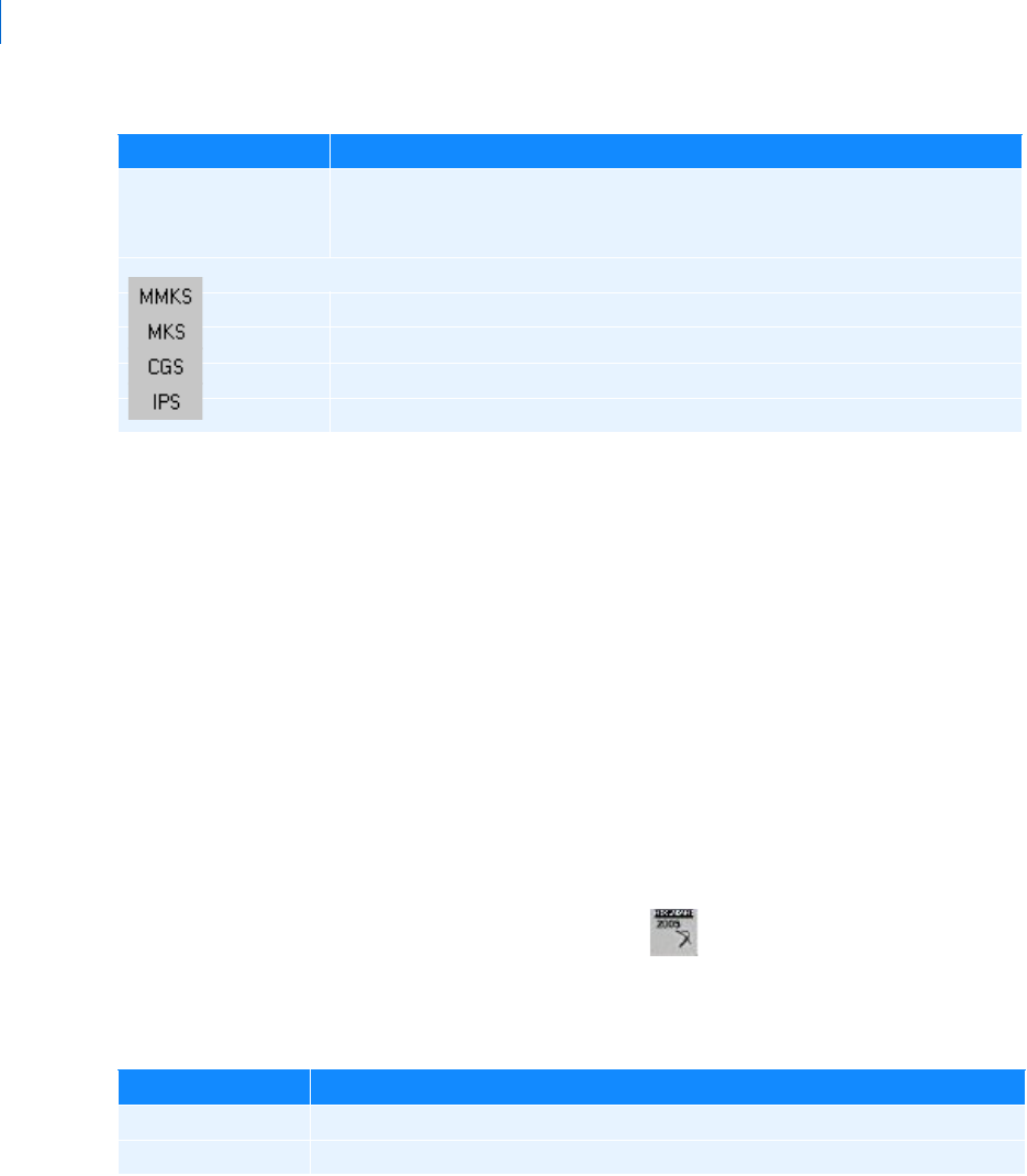
Adams PostProcessor
PPT Preferences
10
PPT Preferences - Stereo
Edit -> Preferences -> Stereo Tab
Sets options for using Adams PostProcessor with stereo viewing. Stereo viewing is available on all Linux
platforms but not Windows. When running Adams PostProcessor, stereo viewing mode cannot be set until
you've displayed an animation. The easiest way to do this is to either load an animation or set the mode to
Animation (in the upper left corner of the window).
In addition, before running Adams, you need to set the MDI_STEREO environment variable
MDI_STEREO (setenv MDI_STEREO 1).
Learn more about setting environment variables.
Stereo viewing is only available when running Native OpenGL graphics with the
OpenGL_Software_Assisted registry setting set to disabled. You use the Registry Editor.
To set this registry setting:
1. From the Adams Toolbar, right-click the Toolbar tool , and then select Registry Editor.
The Registry Editor appears.
2. Select AView -> Preferences -> Graphics -> OpenGL_Software_Assisted.
For the option: Do the following:
Length, Mass, Force,
Time, Angle,
Frequency
Select the units you want or use a preset value below.
The buttons below are preset values. For all preset values, time is in seconds.
Sets length to millimeter, mass to kilogram, and force to Newton.
Sets length to meter, mass to kilogram, and force to Newton.
Sets length to centimeter, mass to gram, and force to Dyne.
Sets length to inch, mass to pound-mass, and force to PoundForce.
For the option: Do the following:
Stereo viewing Select to enable stereo viewing.
Depth of Field Slide to control the depth of the perspective matrix.
11
Setting Preferences
Specifying the Working Directory
Save
Select to save the changes permanently for the next sessions.
If you are using Adams PostProcessor stand-alone, it stores the preferences in the file pptBS.cmd in
your working directory.
If you are using Adams PostProcessor with Adams View, it stores the preferences in the file
aviewBS.cmd. The BS stands for Before Startup, meaning that Adams PostProcessor will read it
before it reads any other setup files.
If Adams PostProcessor finds either pptBS.cmd or aviewBS.cmd in the current working directory or the home
directory, it automatically loads it when it starts up. Since Adams PostProcessor overwrites the file when you
save it during a session, you should not edit it manually.
Restore
Select to restore the settings to their defaults.
Specifying the Working Directory
By default, Adams PostProcessor saves all files in the directory from which you ran Adams PostProcessor. You
can change the working directory.
To change the working directory:
1. From the File menu, select Select Directory.
Eye Separation Slide to control of offset between the left and right modeling views.
Parallax Control the type of parallax view used to display the model:
Positive - Positive parallax viewing produces images that appear to be
within the space of the monitor. For engineering purposes where objects
are often cut off by the window borders or partially obscured by dialog
boxes, positive parallax viewing produces images that are less confusing to
the viewer and are, therefore, easier to view.
Negative - Negative parallax viewing produces images that appear to float
in space in front of the display. Viewing floating images that are partially
obscured by interface items produces confusing cues to the viewer. While
the image appears in front of the screen, the interface items appear to be on
the screen but these interface items can obscure part of the image. These
conflicting inputs can be confusing and lead to extra strain.
Eye Position Use with Negative parallax viewing and use it to control how far the image floats in
front of the screen.
For the option: Do the following:
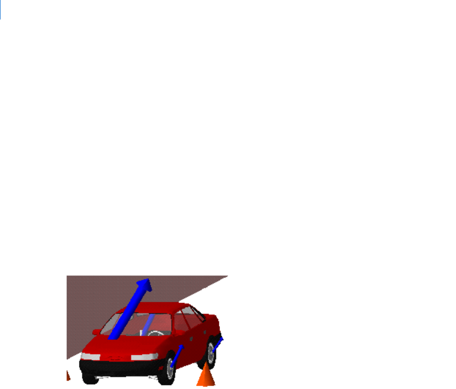
Adams PostProcessor
Part Graphics
12
2. Select the directory in which Adams PostProcessor should save files.
3. Select OK.
Part Graphics
You can set the following for parts:
Part Coordinate Triad - Display a triad that represents the reference frame used to locate and orient
all markers associated with the part.
Center of gravity - Display the center-of-mass
marker for each part.
About Force Graphics
Force graphics are arrows whose magnitudes and directions are proportional to the magnitudes and directions
of the forces acting on your model during a
Simulation. Force graphics help you gauge how large your forces
become and in what directions they are applied during a simulation.
Force Graphics on an Animation
To see force graphics during
Animations, you must specify those force elements in your model for which you
would like to see the associated force graphics. To turn force graphics on or off for particular forces, refer to
the Adams View documentation that describe how to modify a force or a motion.
You can specify the following for the display of force graphics during an animation:
Scale factor used to control the graphic’s relative size compared to the objects in the model.
Whether or not the force magnitudes are displayed numerically. The numerical values appear near
the arrowheads.
Whether or not the force graphics are drawn in Wireframe render mode or Shaded rendering mode when
the model is animated in shaded mode.
Whether the force graphic is always drawn in front of other geometry. This is particularly useful
when viewing forces inside geometry, such as three-dimensional contacts.

13
Setting Preferences
Caching of Animations
There are two different scale factors: one for forces and one for torques. Adams applies the force scale factor
to all force graphics in your model to maintain their proper relative sizing, while it applies the torque scale
factor to all torque graphics in your model.
Finding force and torque scale factors that are good for the entire animation might require some trial and
error. It is often useful to set your scale factors while viewing the frame for which the largest force reaches its
peak value.
Learn more:
Setting Up Force Graphics
Force Graphics Settings Dialog Box
PPT Preferences - Animation
Caching of Animations
When performing Animations that contain Flexible bodies or dynamic geometry, such as spring-dampers, Adams
PostProcessor produces a cache of data as it calculates what the geometry will look like in each frame of the
animation. You can set when Adams PostProcessor produces this cache depending on the amount of memory
in your system and the performance you’d like to see. You can set it to:
Cache the animation before playing it (pre-cache) - Adams PostProcessor caches the data before it
plays the animation. You will see a delay from when you select to play the animation and the actual
start of the animation. This is the default.
Create the cache as it plays the animation the first time - Adams PostProcessor calculates the
geometry as it runs the animation the first time. Therefore, the first time you play the animation it is
slow but subsequent animation loops will be faster.

Adams PostProcessor
Caching of Animations
14
1
Keyboard Shortcuts
Keyboard Shortcuts
The entries on the left show the keyboard shortcuts for Adams View organized by operation. Keyboard
shortcuts allow you to quickly access commonly used commands. The shortcuts available depend on the
current mode (animation or plotting) as well as the location of the cursor.
The shortcuts are organized into the following operations:
Menu Shortcuts
Interface Object Shortcuts
Function Keys
Animation Mode Shortcuts
Plotting Mode Shortcuts
Menu Shortcuts
Interface Object Shortcuts
These keyboard shortcuts work with interface objects, such as the Property Editor, Dashboard, or dialog boxes.
To: Enter:
Print Ctrl + P
Exit Ctrl + Q
Undo Ctrl + Z
Redo Ctrl + Shift + Z
Delete Ctrl + X
To: Enter:
Copy selected text in text boxes Ctrl + C
Cut selected text in text boxes Ctrl + X
Paste cut or copied text in text boxes Ctrl + V
Move focus to next object Ta b
Move focus to previous object Shift + Tab
Adams PostProcessor
2
Function Keys
Animation Mode Shortcuts
Plotting Mode Shortcuts
Selection or Statistics Mode
To: Enter:
Import command file F2
Toggle command window visibility F3
Toggle treeview visibility F5
Toggle dashboard visibility F6
Return to Adams View (Only available in integrated mode) F8
To: Enter:
Set dynamic rotation mode r
Set dynamic translation mode t
Change depth perspective d
Set dynamic zoom mode z
Draw window to zoom w
Pick point to move to center of viewport c
Select element to which to orient viewport e
Set dynamic spin mode (rotate) s
Fit to viewport f
Orient to front Shift + F
Orient to back Shift + B
Orient to right Shift + R
Orient to top Shift + T
Orient to isometric Shift + I
Toggle shading Shift + S
Toggle icon visibility v
Select mode Esc
Interactive highlighting Ctrl (during mouse motion)
Snap to 30-degree increments Shift (during view)
Interactive selecting Ctrl + left mouse button
3
Keyboard Shortcuts
Statistics Mode
To: Enter:
Zoom Click middle mouse button
Fit plot Double-click middle mouse button
To: Enter:
Previous curve Up arrow
Next curve Down arrow
Previous point Left arrow
Next point Right arrow
Previous local maxima Shift + left arrow
Next local maxima Shift + right arrow
Previous local minima Ctrl + left arrow
Next local minima Ctrl + right arrow

Adams PostProcessor
4

5
Examples of Using Adams PostProcessor
Bode Plot Tutorial
Examples of Using Adams
PostProcessor
(Some examples may require internet access)
Tutorials of overall product use:
Getting Started Using Adams PostProcessor
Examples of Adams PostProcessor features:
Bode Plot Tutorial
Defining Filter Function
Adams Verification Guide
Bode Plot Tutorial
This tutorial steps you through an example of how to construct bode plots when using Adams View and
Adams PostProcessor together. It contains the sections:
About the Tutorial
About Example Model’s Input and Output
Investigating the Frequency Response
About the Tutorial
We’ve provided an example command file called bode_tutorial.cmd in the
install_dir\aview\examples\user_guide directory of your Adams installation directory. It
contains an idealized model of a rocket and a payload.
A force with an unspecified thrust function propels the rocket, and the payload interacts with the rocket
though a spring. Both the rocket body and the payload body are constrained to have a single degree of
freedom (DOF) each along the x-axis. A drag force is acting on both bodies.
Figure 1 shows the model.
Note: To run this tutorial, you must use Adams PostProcessor with Adams View. You cannot use
standalone Adams PostProcessr.
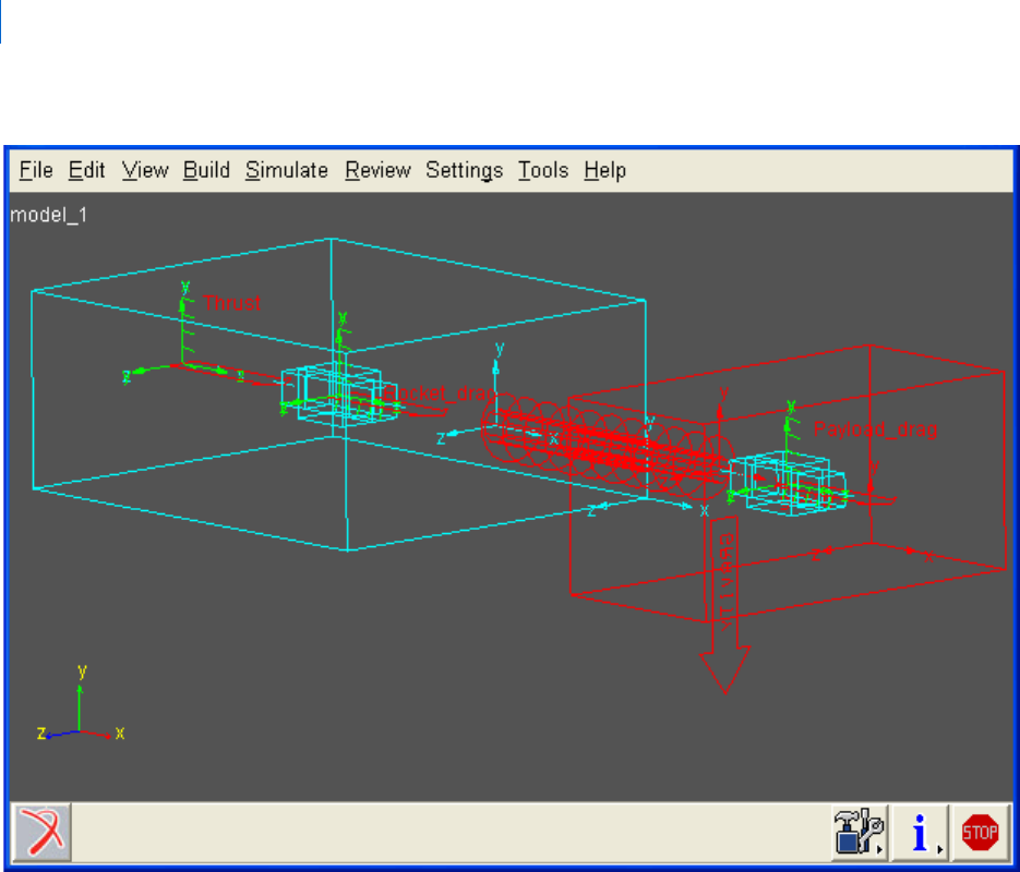
Adams PostProcessor
Bode Plot Tutorial
6
Figure 1 Idealized Model of Rocket and Payload
About Example Model’s Input and Output
The model has a single input and a single output. The system input is a measure of the thrust, and the system
output is velocity of the payload relative to ground.
The force balance equation for the rocket is:
where:
and are the positions of the rocket and payload.
m
1
p
··
1
c
1
p
·
1
kp
1
p
2
–()u=++
p
1
p
2

7
Examples of Using Adams PostProcessor
Bode Plot Tutorial
and are the are mass and drag coefficient for the rocket
k is the connecting stiffness.
u is the thrust.
Dots denote time derivatives.
The force balance equation for the payload is shown below where and are mass and drag coefficients:
Solving the second equation for and substituting the solution in the first equation, you will find, after
some algebra, where the parameterized values denote time derivatives:
Substituting the following parameter values from the example model:
m
1
= 100kg
m
2
= 10kg
c
1
= 20Ns/m
c
2
= 2Ns/m
k = 10N/m
You get the following:
which yields the transfer function:
You can also introduce a change of variables:
and noting that is the output variable y, you can achieve first-order form of the differential equation:
m
1
c
1
m
2
c
2
m
2
p
··
2
c
2
p
·
2
kp
2
p
1
–()0=++
p
1
p
2
4()
m
1
c
21()
c
1
m
2
+
m
1
m
2
-------------------------------------
p
2
3()
km
1
m
2
+()c
1
c
2
+
m
1
m
2
--------------------------------------------
p
2
2()
kc
1
c
2
+()
m
1
m
2
------------------------
p
2
1()
ku=++ +
p
2
4()
0.4p
2
3()
1.14p
2
2()
0.22p
2
1()
0.01u=++ +()d
Ts()
0.01
s
3
0.4s
2
1.14s 0.22+++
------------------------------------------------------------
=
x
3
p
2
3()
=
x
2
p
2
2()
=
x
1
p
2
1()
=
x
1
Adams PostProcessor
Bode Plot Tutorial
8
and an output equation:
The ABCD matrices are evident in the two equations.
In the example, you will investigate the frequency response in the 0.01 Hz to 10 Hz range. You will do so
using four of the seven modes of Bode plots. The remaining three modes are simple extensions of these four.
Investigating the Frequency Response
The command file bode_tutorial.cmd creates the idealized model of a rocket and payload shown in
Figure 1. It defines the following elements for you:
Rocket and payload parts.
Connecting spring, drag, and thrust forces.
Translational joints connecting the two parts to ground.
Plant input element containing the Thrust_value measure that defines the thrust function used
in the thrust force.
Plant output element containing the Payload_velocity measure that defines the velocity of the
payload relative to ground.
In the next sections, you’ll do the following:
Create A, B, C, D matrices, as derived earlier, that analytically describe the system.
Modify the measure Thrust_value so it defines a SWEEP function that applies harmonic
excitation of unit amplitude and a linearly varying frequency.
Run a simulation and generate linear state matrices, using Adams Linear.
Generate Bode plots for each type of construction method.
You must have Adams Linear to run the portion of this tutorial that generates linear state matrices. To
purchase Adams Linear, see your MSC sales representative.
Setting Up the Model
In this section, you’ll import the model, create ABCD matrices for it, and modify the Thrust_value function
measure.
x
·
1
x
·
2
x
·
3
010
001
0.22– 1.14– 0.4–
x
1
x
2
x
3
0
0
0.01
u+=
y
100
x
1
x
2
x
3
0[]u+=

9
Examples of Using Adams PostProcessor
Bode Plot Tutorial
To set up the model:
1. Copy the file /install_dir/aview/examples/user_guide/bode_tutorial.cmd to your
working directory.
install_dir is the directory where the Adams software is installed. If you cannot
locate the directory, see your system administrator.
2. Start Adams View, and import the command file
bode_tutorial.cmd.
3. Create A, B, and C data element matrices as listed below. Because D is a 1 x 1 zero matrix, you do
not need to define it. As you create the matrices, name them A, B, and C, use full format, and order
the matrices by row. For complete instructions on creating matrices, the Adams View online help.
• A is a 3 x 3 matrix input with the values:
0.0, 1.0, 0.0,
0.0, 0.0, 1.0,
-0.22, -1.14, -0.4
• B is a 3 x 1 matrix with the values:
0.0
0.0
0.01
• C is a 1 x 3 matrix with the values:
1.0, 0.0, 0.0
4. Create a thrust function by modifying the
Thrust_value function measure to the following:
sweep(time,1.0,1.0,.001,100.0,1.0,0.01)
The thrust function defines a frequency sweep function that applies harmonic excitation of unit
amplitude and a linearly varying frequency starting at 0.001 Hz at 1 second and increasing to 1 Hz
at 100 seconds with a 0.01 second lead to smooth the transition. Note the parallels to a shaker table.
For complete instructions on modifying a measure, see Defining Output Using Measures in the
Adams View online help.
Simulating the Model
Now you’ll simulate the model and construct linear state matrices. You can only construct linear state
matrices if you have Adams Linear. If you do not have Adams Linear, you can still proceed with the rest of
the tutorial.
Note: By default on Windows, files in the installation directory are read-only. During
installation, your system administration can choose to change the permissions so you
can write to the installation directory. If this has not been done, you will need to
change the permission of the above file when you copy it to your working directory.

Adams PostProcessor
Bode Plot Tutorial
10
To simulate the model and construct matrices:
1. Simulate the model for 100 seconds with 1023 output steps, for a total of 1024 (a power of two)
output points.
2. Construct linear state matrices by linearizing the system at its state at 100 seconds if you have Adams
Linear. If you do not have Adams Linear, continue to the next section.
To linearize the system:
a. From the Simulation Controls dialog box, select the Linear State Matrix tool .
b. In the dialog box that appears, enter the plant input and output. Double-click the text boxes to
display the Database Navigator.
c. Select OK.
Constructing Bode Plots
You are now ready to construct Bode plots of the system for linear state matrices, ABCD matrices, transfer
function coefficients, and measures.
To construct Bode plots:
1. Display the plotting window.
2. On the Plot menu, select Bode Plots.
The Bode Plot dialog box appears.
3. From the Input Format option menu, select Adams Linear State Matrices if you computed state
matrices in the previous section. If you did not, continue with Step 5.
4. Enter the Linear State Matrix results object, and request a frequency range of 0.01 to 1 with 100
logarithmically spaced output points. Select Apply.
The Bode plots appear in the plotting window as shown in
Figure 2. The plot shows the accumulated
curves.
5. Now, from the Input Format option menu, select Adams Matrices. Browse for the A, B, and C
matrices defined earlier. Leave the D text box blank and choose the same frequency sampling as in
Step 4. Select Apply.
The Bode plots appear in the plotting window as shown in
Figure 2. The plot shows the accumulated
curves.
Note: In this example, the number of output steps is a power of two minus one. By
specifying an even power minus one, the number of data points in the results is a
power of two (the output steps you requested plus one for the model’s initial
condition). While this is not required, we recommend you do so to obtain peak
performance for Bode calculations. For more information on simulating models in
Adams View, see the Adams View online help.
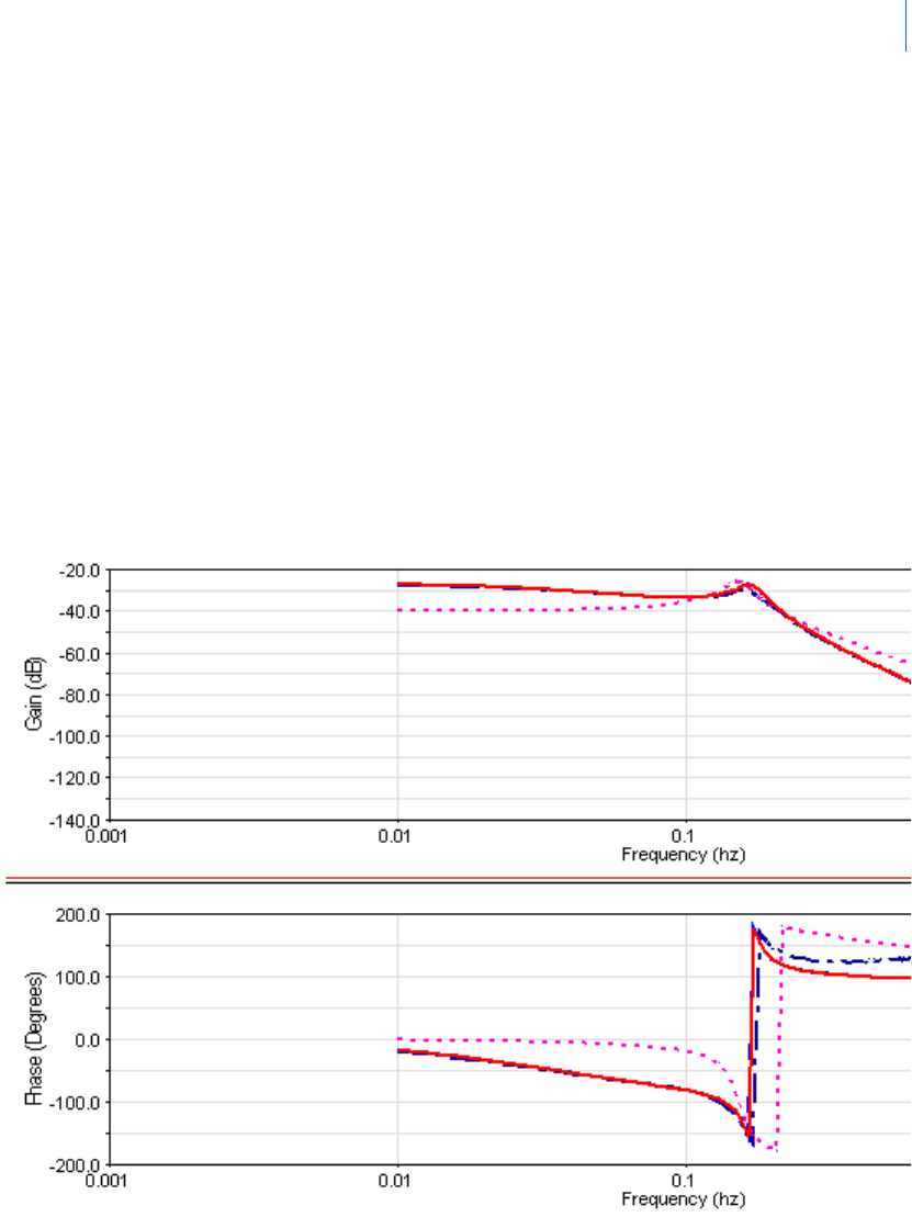
11
Examples of Using Adams PostProcessor
Bode Plot Tutorial
6. From the Input Format option menu, select Transfer Function Coefficients, and select the
numerator coefficient of 0.01 and denominator coefficients of 1.0, 0.4, 1.14, and 0.22. Choose the
same frequency sampling as in Steps 4 and 5. Select Apply.
The Bode plots appear in the plotting window as shown in
Figure 2. The plot shows the accumulated
curves.
7. Finally, from the Input Format option menu, select Time Domain Measures. Then, browse for the
Thrust_value measure as input and the Payload_velocity measure as output. Because the frequency
range is controlled by the time resolution of the input signals, no frequency control is available. Select
OK.
The Bode plots appear in the plotting window as shown in
Figure 2. The plot shows the accumulated
curves.
Notice how all the four sets of curves agree in their results except for the one generated by measure
data, which is slightly less accurate. You could improve the accuracy of this curve by requesting
additional outputs in Step 4.
Figure 2 Bode Plot for Example Model

Adams PostProcessor
Bode Plot Tutorial
12
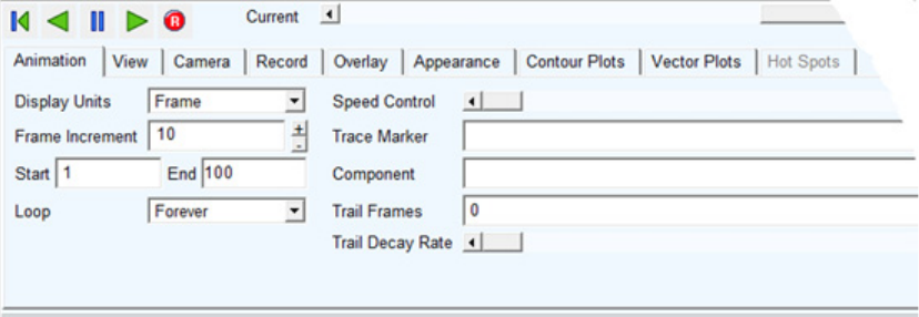
Dialog Box - F1 help
Animation Dashboard
The dashboard in animation mode (see Modes) lets you play and control time- and frequency-domain
animations, record them, and view
Contour plots and Vector plots.
See
Types of Animations.
Time-based Animations
Animation Dashboard - Animation
Animation Dashboard - View
Animation Dashboard - Camera
Animation Dashboard - Record
Animation Dashboard - Overlay
Animation Dashboard - Appearance
Animation Dashboard - Contour Plots
Animation Dashboard - Vector Plots
Animation Dashboard - Hot Spots
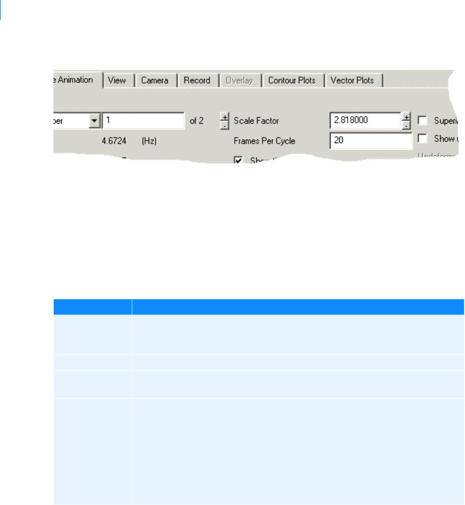
Adams PostProcessor
Animation Dashboard - Animation
16
Frequency-based Animations
Adams Vibration Animations
See Animation Dashboard - Vibration Animation .
Animation Dashboard - Animation
Load Animation -> Animation dashboard -> Animation tab
Lets you play and control Time-domain animations.
For the option: Do the following:
Display Units Set whether to control animations based on their frame numbers or time. For
example, to view an animation between 3.0 and 5.5 seconds, you would set Display
Units to time, and then set the start time to 3.0 and the end time to 5.5.
Frame Increment Select the number of frames to skip when playing an animation.
Start/End In the Start text box, enter the starting frame or time, depending on the value of
Display Units (see above), and in the End text box enter the ending frame or time.
Loop Set how Adams PostProcessor plays the animation:
Forever - Continuously loop through the animation.
Once - Animate one time.
Oscillate - First play the animation forwards and then play it backwards (for
example, in a 100-frame animation, animate from 1 to 100 then back from
100 to 1).
Oscillate forever - Oscillate forward and backward repeatedly.
17
Dialog Box - F1 help
Animation Dashboard - Animation
Animation Type This option determines how plot's curve(s) will be drawn as time moves forward. It
has following two options:
1. Advancing Curve: Includes a sub-option “Time Window (sec)” by which a
moving window of time can be specified (for example, display on the last 5-
seconds of time). Plot's curve(s) will be drawn in a way where h-axis has range
of values equivalent to time window, if specified, and curve will be displayed
in accordance with time value.
Note: 4D Plotting does not support Advance curve option.
2. Time Marker: Plot's curve(s) will be displayed as per the axes limits. In
addition, a vertical line with a symbol tracing curve's value at a particular will
be displayed at a given frame.
Speed Control Change the speed at which time-domain animations play. Speed Control introduces
a time delay between each frame of an animation. The default, when the slider is all
the way to the right, is to play each animation as fast as possible. Moving the slider to
the left introduces a time delay of up to 1 second.
Trace Marker Enter the names of one or more Markers for which you want Adams PostProcessor to
generate paths during a time-domain animation.
Tips on
Entering Object Names in Text Boxes.
Learn more about
Tracing the Paths of Points in Time-Domain Animations.
Component Enter the name of the flexible body or rigid stress object you want to animate. No
other parts will be displayed. This allows you to display only one body at a time.
The bodies appear without any of the translational or rotational information from the
analysis. This allows you to focus in on contour plot information, as well as the hot
spot information for both flexible and rigid stress objects. Also, with flexible bodies,
the component view allows you to watch its deformations within the animation.
Trail Frames Enter the number of successive frames of a time-domain animation to overlap. This
helps you to better visualize the motion of a model or to add a sense of motion to still
images of the animation.
Picture of Trailing Frames
You can control the decay rate using the Trail Decay Rate slider (see next).
Trai l D e c a y R a t e Slide to set the rate at which Adams PostProcessor no longer displays trailing frames.
By default, the slider is all the way to the left, specifying no decay.
Superimpose Select to superimpose successive frames of a time-domain animation. When you
toggle the Superimpose button, Adams PostProcessor accumulates each frame.
Picture
of superimpose
For the option: Do the following:

Adams PostProcessor
Animation Dashboard - Camera
18
Animation Dashboard - Camera
Animation dashboard -> Camera tab
Lets you change your viewing or camera perspective. For example, you can change the perspective to always
look at a particular part as it moves or to always look from a particular vantage point, such as one that moves
with a part. Setting different camera perspectives is particularly helpful when parts undergo large motions
and move off your screen during an animation, such as with vehicle simulations.
A good example of setting the camera perspective is when you simulate a vehicle driving through a slalom
course on a test track. By default, you view the simulation as a bystander alongside of the road whose gaze is
fixed in one direction. As the vehicle moves forward, it quickly moves out of your field of view. You can,
however, set the camera perspective to mimic the movement of your head as it moves to follow the vehicle.
Furthermore, rather than observe the vehicle as a bystander alongside a road, you can also set the camera
perspective to mimic what the driver sees as he or she looks out the front windshield of the vehicle.
Tips for
Specifying the Camera Perspective.
Include Static Select to display the frames representing static equilibrium of time-domain
animation.
Continue selecting Next Static to view all static equilibrium positions.
Include Contacts Select to display the frames representing contacts. By default, Adams PostProcessor
does not display intermittent contact frames that two- and three-dimensional contacts
produce to avoid the illusion of deceleration during animations.
Continue selecting Next Contact to view all contacts between parts.
Model Input Select to display the frame representing the model input. Model input represents the
state that the model is in before the simulation. It does not account for assembly initial
conditions or static solutions.
Next Static (Available if you selected Include Static.) Select to display the next frame representing
static equilibrium.
Next Contact (Available if you selected Include Contacts.) Select to view all contacts between parts.
For the option: Do the following:
For the option: Do the following:
Tips on Entering Object Names in Text Boxes.
Follow Object Enter the marker that you want to follow. See Markers.
Mount Camera At Enter a marker from where you want the camera vantage point.
Lock Rotations Select to follow the rotations of the followed object.
19
Dialog Box - F1 help
Animation Dashboard - Contour Plots
Animation Dashboard - Contour Plots
Animation dashboard -> Contour Plots tab
Lets you set up the options for displaying Contour plots. For each viewport (see Viewports), you can change the
way contour plots display colors and values. Note that this allows you to display different viewports at the
same time but with different color values, which can be confusing because a color value in one viewport may
not be the same as in another.
Learn more about contour plots with
Animating Deformations, Modal Forces, and Stress/Strain.
Animation Dashboard - Hot Spots
Animation dashboard -> Hot Spots tab
Lets you display hot spots in your Adams Durability animation. Learn more about Visualizing Hot Spots.
For the option: Do the following:
Display Legend Select to turn on the display of legend.
Contour Plot Type Select the type of contour plot to display. The type of plot depends on the analysis
data. You can display deformation data from Adams Flex, stress and strain data from
Adams Durability, and modal force (MFORCE) data from Adams Flex and Adams
View, and kinetic energy from Adams Vibration.
Legend Placement Select where you'd like the legend to appear.
Legend Title Change the text of the legend title.
Colors Enter the number of colors to be displayed in the plot. There can be no more than
255.
Legend gradients Enter the number of color gradients shown in the legend.
Minimum Value Enter the minimum value for the plot.
Maximum Value Enter the maximum value for the plot.
Reset Limits Select to reset the legend values based on the flexible bodies in the active view.
Decimal Places Enter the number of decimal places to which the numbers in the legend should be
displayed.
Scientific Range Enter the exponential form for scientific notation.
Trailing Zeros Select to have Adams PostProcessor display zeros after the numbers in the legend. The
number of zeros depends on the number of decimal points you selected for Decimal
Places.
Adams PostProcessor
Animation Dashboard - Mode Shape Animation
20
Animation Dashboard - Mode Shape Animation
Load Mode Shape Animation -> Animation dashboard -> Mode Shape Animation tab
Lets you play and control animations for Frequency-domain animations.
For the option Do the following
Display Hotspots Select to display the hot spots in your animation.
Sort Order Specify one of the following sorting options:
Absolute - The sign of the value is ignored when sorting hot spots.
You would use this option when only the magnitude is important and
not the sign or direction (in the case of stress or strain).
Maximum - Hot spots are ranked from maximum to minimum.
Minimum - Hot spots are ranked from minimum to maximum.
Filter/Value Select the type and number of hot spots to display:
Node Count - Enter the number of top hot spots to display.
Threshold - Display only those hot spots that meet or exceed this
value.
Percentage - Specify the number of hot spots to display as a
percentage.
Radius Enter the distance between hot spots. All nodes that fall within this radius are
candidates for the same hot spot. A value of 0.0 considers all nodes to be
potential hot spots.
Graphics Label Contents Select the display of hot spot labels:
Rank - Displays the sorting order of each hot spot.
Value - Displays the value of each hot spot.
Frame - Displays the frame when the value occurred.
Node ID - Displays the node ID for that hot spot.
Note: 1. If you do not select any of these options, Adams PostProcessor
only displays a cross hair at each hot-spot location.
2. The color of the hot-spot graphics is the same as the flexible body
color.
3. Hot-spot graphics can be hidden by other graphics. For better
viewing of hot spot graphics try rotating the display, making the
flexible body transparent, or displaying only one body at a time using
the Component display feature in the Animation tab.

21
Dialog Box - F1 help
Animation Dashboard - Mode Shape Animation
For the option: Do the following:
Mode Number/Frequency Select one of the following:
Mode Number - Enter the mode number you want to view. You
can also use the +/- buttons to move through all the modes.
Frequency - Enter the frequency of the mode you want to view.
If you specify the frequency, Adams PostProcessor uses the mode closest to
the specified frequency. If you specify neither the mode nor the frequency,
Adams View deforms the model using the first mode.
Scale Factor Specify the amount parts translate or rotate from their undeformed
position. If you do not specify a scale factor, Adams PostProcessor translates
parts no more than 20 percent of model extent and 20 degrees. You can
adjust the value using the +/- buttons, which increases or decreases by 10%
each click.
Frames Per Cycle Enter the number of frames to be displayed for each cycle. Adams
PostProcessor performs the interpolation between the frames using
trigonometric functions; therefore, the frames tend to be segregated at the
maximum deformation in the positive and negative directions.
Note: A full cycle goes from undeformed, to maximum positive
displacement, back to undeformed, then to maximum
displacement in the negative direction, and finally back to
undeformed.
Show Time Decay Specify whether the amplitudes of the deformations are to remain constant
or decay due to the damping factor calculated in the eigensolution.
Small Angle Approximation Select to toggle between the current animation mode and the other
animation mode. If your parts are expanding/contracting excessively due to
rotational modes, you may want to uncheck this box and view the other
animation mode.
Adams PostProcessor
Animation Dashboard - Overlay
22
Animation Dashboard - Overlay
Animation dashboard -> Overlay tab
Lets you play one animation on top of another animation. To help you see the two animations, you can
change their color and offset one from the other. You'll find this helpful when you want to visually compare
the results of two or more modeling changes.
Superimposed Select to show each mode superimposed on the other modes.
Show undeformed/
Undeformed Color
Select to display the undeformed part of your model with the deformed
shape superimposed on top of it. If you select to show the undeformed,
specify the undeformed color. If you do not specify a color, Adams
PostProcessor displays the undeformed model using the same color as the
deformed mode.
Table of Eigenvalues Select to display an Information Window with the eigen values for each
mode.The information includes:
Mode number - Sequential number of the mode that the
eigensolution predicted.
Frequency - Natural frequency corresponding to the mode.
Damping - Damping ratio for the mode (the log decrement is
another way to represent this quantity).
Eigenvalues - List the real and imaginary part of the eigenvalue.
For the option: Do the following:
Note: Each animation you overlay must have the same beginning, increment, and end times.
For the option: Do the following:
Analysis From the list, select the animations to be overlayed.
Offset Enter the amount by which to offset the animations. Enter x, y, and z values. Adams
PostProcessor applies the offset to each animation if you selected more than two
animations to overlay.
Colors Enter the colors in which to display the overlaid animation.
Tips on
Entering Object Names in Text Boxes.
23
Dialog Box - F1 help
Animation Dashboard - Record
Animation Dashboard - Record
Animation dashboard -> Record tab
Lets you set up the options for recording an animation as a series of files, each containing one frame of the
animation. Adams PostProcessor saves the files to your current working directory. Once you've recorded the
animation, you can import the images into a third-party multimedia tool to create movies.
If the simulation control or animation control dialog box is in opened state in Adams View, close it before
movie recording start.
To record the animation:
From the dashboard, select , and then select .
For the option: Do the following:
File Name Set the prefix used to name the set of files. Adams PostProcessor appends a unique
number to the prefix to form the name of each file. For example, if you specify a
prefix of suspension, then each .tif file is named suspension_0001.tif,
suspension_0002.tif, and so on. If you do not specify a name, the prefix is frame
(for example, frame_001.tif).
Format Select the format: .avi, .tif, .jpg, .bmp, .mpg, .png, and .xpm (AVI format is only
available on Windows).
Frame Size Select to define an area of the viewport (see Viewports) to record according to the
values in Width and Height (see below). If the frame size exceeds the area currently
on the screen, a warning message appears. You can fit the frame on the screen by
resizing the dashboard, hiding toolbars, or increasing the size of the Adams
PostProcessor window. Tip on
Resizing and Resetting Interface Objects.
Width/Height Define the frame of the animation (see above).
Next options are for AVI format only:
Movie replay rate Set the frame rate.
use compression Turn off compression to improve the quality of the images. The default is
compression.
Note: When you set use compression when recording in AVI format, the
playback program may restrict the size of image frames, usually to a
multiple of 2 or 4. Therefore, your recording may appear cut off on one
or more sides. The workaround is to change the animation window size
before recording.
Adams PostProcessor
Animation Dashboard - Appearance
24
Animation Dashboard - Appearance
Animation dashboard -> Appearance
Key frame every Set the interval between key frames. The default is a key frame every 5000 frames.
Note: When a digital movie stream is encoded with compression, the pixels of
each frame are evaluated against previous frames (those designated as
key) and only pixels that changed are stored. For example, a movie of a
car traveling along a road can have many pixels in the image
background that do not change during the entire movie. Therefore,
storing only the pixels that change allows for significant compression. In
many cases, however, it can degrade movie quality, especially with
movies where a large percentage of pixels are changing from frame-to-
frame, such as with wireframe graphics. Because Adams PostProcessor
lets you set the key frame rates, you control both the compression factor
and the movie quality.
Movies with many key frames will have high quality, while movies with
few key frames, such as the default every 5000 frames, will have lower
quality. For a typical 20-second AVI movie of a shaded Adams model, a
key frame rate would be 12.
Quality Enter a value or use the slider to set the image quality.
Next options are for MPG format only:
Tip:
Configuring Browser to Play MPEG Video
Running MPEG Movie Using Windows Media Player
Compress Using P
Frames
Turn off the compression using P frames to ensure your movie plays in many
playback programs, including xanim. It results, however, in a much larger file (up
to 4 times as large).
Round Size to
Multiplies of 16
Some playback programs require the pixel height and width to be multiplies of 16.
Turning this option on ensures that your movie plays in many playback programs.
For the option: Do the following:
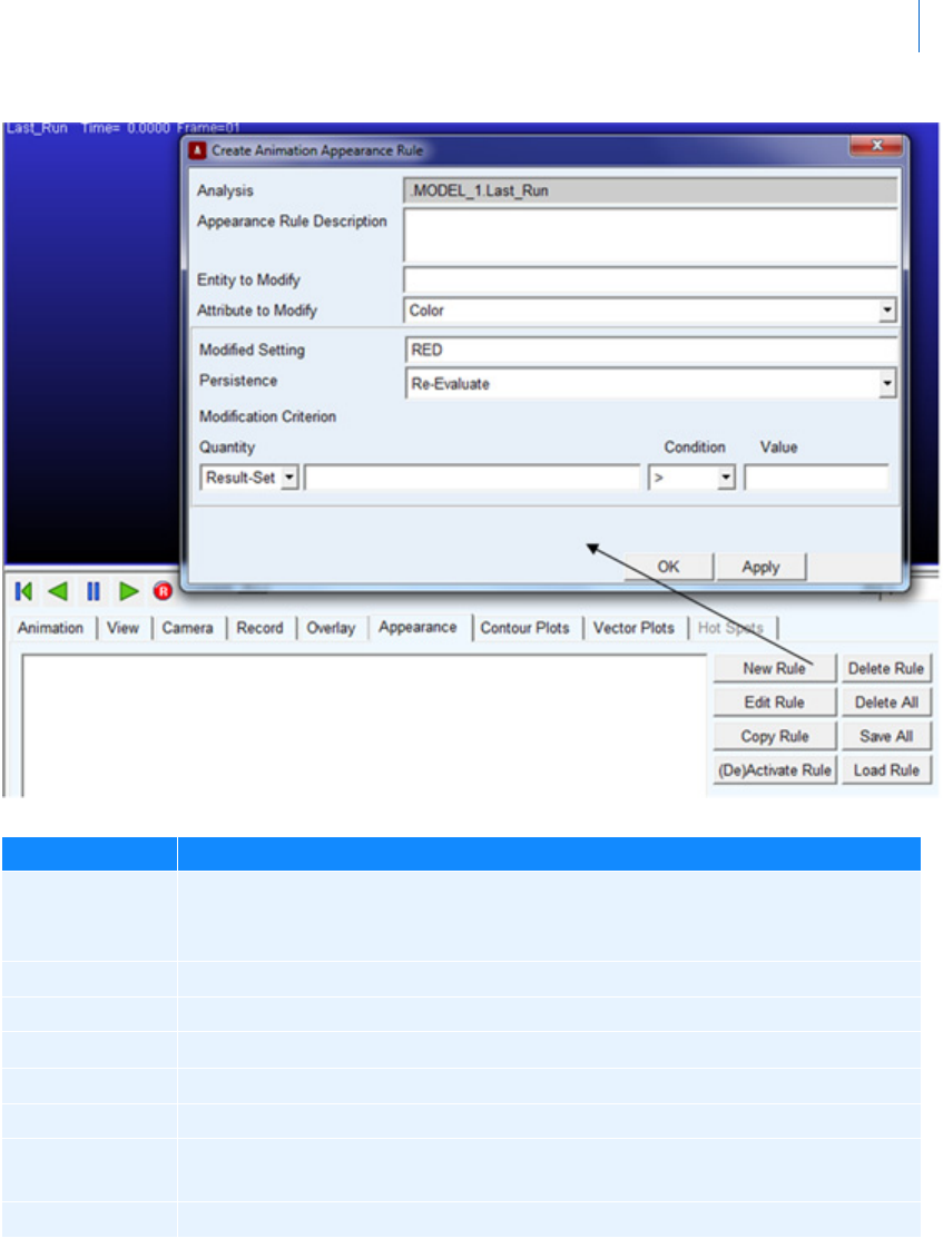
25
Dialog Box - F1 help
Animation Dashboard - Appearance
For the option: Do the following:
New Rule Launches the Create Animation Appearance Rule dialog box which allows you to modify
the appearance of geometry during an animation based on conditions of result set
components.
Edit Rule Launches the Modify Animation Appearance Rule dialog box.
Copy Rule Creates a copy of the selected rule (use the Edit Rule button to rename it).
(De)Activate Rule Toggles the active/inactive status of the selected rule.
Delete Rule Deletes the selected rule.
Delete All Deletes all rules in the session.
Save All Saves all rules in the session to an .xml file which can be reloaded later or in other
sessions.
Load Rule Loads the rules in a previously saved .xml rule file.
Adams PostProcessor
Animation Dashboard - Tire/Road
26
Animation Dashboard - Tire/Road
1
Animation dashboard → Tire/Road tab
Lets you overlay wheel/tire forces with the detailed FTire animation files including tire deformation. The
Tire/Road Tab is only activated if FTire animation files (file extension .ogl or .rgu) have been created during
the simulation and graphics option is set to OpenGL/Native.
The FTire wheel/tire forces and deformations are stored in an .ogl file. You can create this file by selecting
Cosin Animation File (.ogl) under Settings
→ Solver → Output to Yes.
The Road Deformation is stored in an .rgu file. You can create this file by selecting Soft Soil Deformations
(.rgu) under Settings
→ Solver → Output to Yes.
1
Adams Car only
Note: The .rgu file is only created when using soft soil roads and a Cosin License ('ftsoil') is available.
For the option: Do the following:
The following option is available for Overlay Animation Settings:
Display Overlay
Animation
Select to overlay the .ogl animation on the Adams animation. The tires of the Adams
model are hidden and tires from the .ogl file are displayed.
The following options are available for both Overlay Animation Setting and Video File Animation Settings:
Display Tire
Forces
Select to display the tire forces from the .ogl animation. Following colors are used:
red: contact element sticking to ground (local sliding velocity smaller than tire-
file-dependent threshold)
yellow: sliding
Display Rim Select to display the tire rim graphics from the .ogl animation.
Display Road
Patch
Select to display the road patch from the .ogl animation.
Note: Road patches are only created if specified in the FTire property file as
animation detail (you can do this by creating the FTire property file using
Cosin/Tire tools, select animation&sound and check, for example,
road:grid)
Select Axle/Tire Select for which axle/tire to overlay the .ogl animation on the Adams animation.
27
Dialog Box - F1 help
Create/Modify Animation Appearance Rule
Create/Modify Animation Appearance Rule
Animation dashboard -> Appearance -> New/Edit Rule
Allows you to modify the appearance of geometry during an animation based on conditions of result set
components.
The following options are available for Road Animation Settings:
Road
Deformation
Select to display the road deformation from the .rgu animation.
Note: The .rgu file is only created when using soft soil roads and a Cosin License
('ftsoil') is available.
Road Grid Scale Scale the road grid dimensions.
For the option: Do the following:
For the option: Do the following:
Analysis Select the analysis for which the rule should apply.
Appearance Rule
Description
Enter text to name the rule.
Entity to Modify Select the geometry object in the model whose appearance is to be controlled by this
rule.
Attribute to
Modify
Select the which appearance attribute is to be controlled by this rule
If Attribute to Modify is set to Color, the following lists appear:
Modified Setting Select the new color which the geometry should have based whenever the
modification criterion is met.
Persistence Permanent: once the modification criterion is met for the first time, the modified
setting will be applied throughout the remainder of the animation.
Re-Evaluate: the modified setting will be applied only for those frames in which
the modification criterion is met; so, for example, the attribute could switch
between default setting and modified setting multiple times during the analysis.
Modification
Criterion
Quantity - Select the type of output that will be used as the modification
criterion, then browse for the specific output item.
Condition - Select the condition which will trigger the appearance modification.
Value - Select the value which will trigger the appearance modification.
If Attribute to Modify is set to Transparency, the following lists appear:
Adams PostProcessor
Animation Dashboard - Vector Plots
28
Animation Dashboard - Vector Plots
Animation dashboard -> Vector Plots tab
Lets you set up the options for Vector plots.
Learn more about vector plots with
Animating Deformations, Modal Forces, and Stress/Strain.
Animation Dashboard - Vibration Animation
Animation dashboard -> Vibration Animation tab
Lets you play and control animations for your Adams Vibration model.
Transition Scale - use this option to gradually move from the current transparency setting to
the modified setting linearly over time.
Immediate - use this option to immediately move the current transparency setting
to the modified setting based on the modification criterion.
If Transparency is set to Scale, the following lists appear:
Modification
Criterion
Choose to use time or animation frame as the independent variable controlling
transparency
Transparency
Setting
Enter transparency settings from 0 (opaque) to 100 (invisible) for the start time/frame
and the end time/frame
If Transparency is set to Immediate, the following lists appear:
Modified Setting Select the new transparency which the geometry should have based whenever the
modification criterion is met.
Persistence Permanent: Once the modification criterion is met for the first time, the modified
setting will be applied throughout the remainder of the animation.
Re-Evaluate: The modified setting will be applied only for those frames in which
the modification criterion is met; so, for example, the attribute could switch
between default setting and modified setting multiple times during the analysis.
Modification
Criterion
Quantity - Select the type of output that will be used as the modification
criterion, then browse for the specific output item.
Condition - Select the condition which will trigger the appearance modification.
Value - Select the value which will trigger the appearance modification.
For the option: Do the following:
For the option: Do the following:
Vector Plot Type Select the type of vector plot to display. The type of plot depends on the modal force
(MFORCE) data from Adams Flex and Adams View.

29
Dialog Box - F1 help
Animation Dashboard - Vibration Animation
For the option: Do the following:
Normal Mode/Forced Vibration
Animation
Select the type of animation you want to view:
Normal Mode Animation
Forced Vibration Animation
If you select Normal Mode Animation, Adams PostProcessor displays the following text boxes:
Mode Number/Frequency Select one of the following:
Mode Number: Specify the mode number you want to view.
Frequency: Specify the frequency value you want to view.
Damping Ratio Enter the damping ratio for the mode (the log decrement is another
way to represent this quantity).
Frames Per Cycle Enter the number of frames to be displayed for each cycle.
Show Time Decay Specify whether the amplitudes of the deformations are to remain
constant or decay due to the damping factor calculated in the
eigensolution.
If you select Forced Vibration Animation, Adams PostProcessor displays the following text boxes:
Frequency Enter the frequency value in the text box or use the slider to select a
value. To specify a value based on a spec line, right-click this text box,
point to Spec_ Line, and then select the spec line you want to use. Once
selected, Adams PostProcessor will put its X value in the Frequency text
box. Learn more about
Adding Spec Lines.
End Time Enter the end time for the animation.
Time Increment Enter the time increment for the animation.
Automatically set time fields for
one cycle
Select to have Adams PostProcessor set the end time and steps for the
forced vibration animation so that one cycle is always displayed. If you
select this option, the End Time and Time Increment text boxes are no
longer available.
Auto Scale Select to have Adams PostProcessor automatically set the minimum and
maximum values.
Adams PostProcessor displays the following text boxes for both animation types:
Scale Factor Specify the scale factor. The default is model dependent. You can adjust
the value using the +/- buttons, which increases or decreases by 10%
each click.
Small Angle Approximation Select to toggle between the current animation mode and the other
animation mode. If your parts are expanding/contracting excessively
due to rotational modes, you may want to uncheck this box and view
the other animation mode.
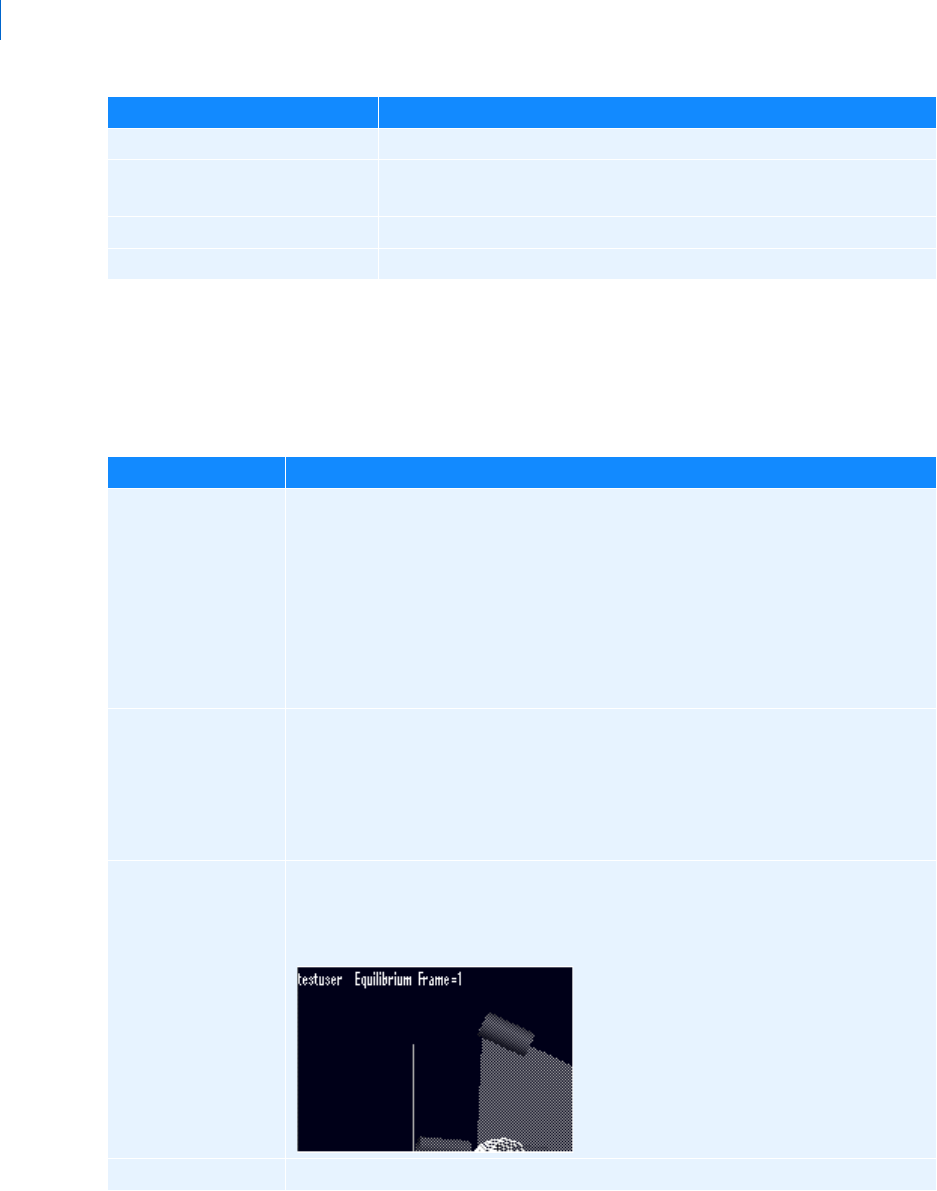
Adams PostProcessor
Animation Dashboard - View
30
Animation Dashboard - View
Animation dashboard -> View tab
Lets you set the display of animations in the Viewports.
Superimposed Select to show each mode superimposed on the other modes.
Show undeformed Select to display the undeformed part of your model. If selected, specify
the undeformed color.
Table of Eigenvalues Select to display the Eigen Information dialog box.
Modal Info Select to display the Modal Information dialog box.
For the option: Do the following:
For the option: Do the following:
Display Icons Select to display Screen icons during animations. Displaying icons can be very
helpful when debugging your model. For example, displaying screen icons during
animations allows you to see if joints or forces applied to parts are behaving as
expected because you can see their icons move as the animation progresses.
Displaying screen icons can also help you see how
markers move during animations
because they control the locations and directions for constraints and forces.
Note that if you import your animation through a
Graphics file (.gra) only, you do
not have joint or force icons.
Perspective Select to change the depth of the screen to perspective projection. Perspective
projection causes a vanishing point effect by showing the size of parts relative to
their distance from the viewer. It does not show the true proportions of all parts. (By
default, Adams PostProcessor displays your animation or three-dimensional plot as
though it were drawn on a flat piece of paper. This is called orthographic
projection.) Learn more about
Setting the View Perspective.
Title Select to display a title for the animation in the upper left corner of the viewport. It
displays the name of the model and the current frame number. During the
animation, it displays the time.
FPS Title Select to add the number of frames per second to the end of the title.
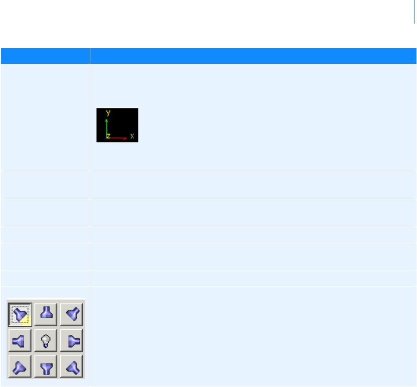
31
Dialog Box - F1 help
Bearing Life
Bearing Life
Tools -> Bearing Life
Bearing Life option in Tool menu is visible only if there is Adams Machinery or Adams Machinery-Bearing
License feature.
Display Triad Select to display a triad that displays the orientation of the global coordinate system
axes:
It appears in the lower left corner of a viewport. As you move the view of a viewport,
the triad displays the changes to the coordinate system orientation.
Light Intensity Set to the amount of overall intensity of the light (much like setting a dimmer
switch in your home).
Ambient Light Set to the amount of background, ambient light to control the diffusion of light
sources to affect the amount of lighting on edges.
Light Angle Use the Light Angle slider to set how far from the center line the light source is.
Light Reflections Select to have reflections off of parts. (Note that this is computationally expensive
and can slow down your animations.)
Two-Sided Lighting Clear to set up one-side lighting. The default is two-sided lighting.
Use the light buttons on the right side of the dashboard to turn on different focused
light sources. Click a light button on the left to see examples of different lighting.
Note: The number of light sources you can select depends on the graphics
driver and system you are using. If you selected OpenGL, the number of
light sources depends on your graphics card. For more information on
selecting graphics drivers, see
Running and Configuring Adams.
For the option: Do the following:
Adams PostProcessor
Bearing Life
32
Formula to calculate service life over the course of the duty cycle
Adams Machinery Bearing calculates a service life estimate at every output step which can be interpreted as
the as the predicted service life in hours for the bearing under the loading and rotational speed conditions at
that output step. See
Bearing Output for details of the inputs to this calculation and Calculation of service life based
on the bearing inner geometry (ISO/TS 16281)
as for details of the life calculation method according to ISO/TS
16281. The single-value service life estimate provided by this "Adams Machinery Bearing Duty-Cycle Service
Life" tool aggregates these individual service life output values from each output step (known as L
i
in the
formulation description, below) over the course of the duty-cycle specified in the dialog box. The formulation
used to accomplish this amounts to an "equivalent life" calculation and is described below:
For the option: Do the following:
Analysis Select the analysis to perform this calculation.
Bearings A multi-select field in which you can select one/more/all of any of the bearings
within the model corresponding to the selected analysis. The bearing must be
modeled via the "Detailed" modeling method option.
Start Time, End Time Real number entries for start and end time.
Start time should be less than end time.
Both should be within the time range for which the analysis was run.
Number of Repeats The number of times this time range in the analysis, as specified by start time and
end time, should be repeated for the life calculation. This must be positive
integer value and greater than 0.
Insert Inserts a row above the selected row (row selection is done by clicking the row
number).
Delete Deletes the selected row (row selection is done by clicking the row number).
File Name Optional:
If no name provided then no file is exported.
If name provided then file will be saved in current working directory with
given name.
File Format "HTML" or "Tab Delimited Text".
Base Font Size Control the font size for the HTML option.
Report The resulting report will be displayed in the upper-side and updated upon each
subsequent click of "Report" button.
Notes: You can save the bearing duty cycle generated report in .html or .txt format.
You can load the report in Postprocessor window.
33
Dialog Box - F1 help
Gear Contact Pattern
Where:
• L
tot
: single-value service life estimate provided for each bearing by this "Adams Machinery
Bearing Duty-Cycle Service Life" tool in units of hours.
• t
i
: time length of the Adams output step in hours. For example, if the time from the previous
output step to the current output step (the current output step is the one from which Li is
taken) is 0.1s, then ti would be 0.1/3600 = 2.778e-5 hours.
• r
i
: the number of repeats applied to the given output step as defined in the duty cycle
specification.
• L
i
: the given output step's life prediction value. It is reported in units of hours.
For more details see "
Adams Machinery Bearing Duty-Cycle Service Life within Adams PostProcessor".
Gear Contact Pattern
Tools -> Gear Contact Pattern
L
tot
t
i
r
i
×() t
i
r
i
×()L
i
⁄[]
⁄
=
For the option: Do the following:
Analysis 'Last_Run' or analysis for which Contact pattern need to be plotted.
It automatically populates 'maximum time' and 'minimum time' fields.
Gear Force Gear force for which contact pattern need to be plotted. The working
directory contains the LPT file generated with same name as that of gear force.
All results are derived from this LPT file.
Minimum/Maximum
Time
Time frame for which results need to be plotted.
Selecting Analysis “RUN” select sets it to Start-End of simulation time.
You can override this value.
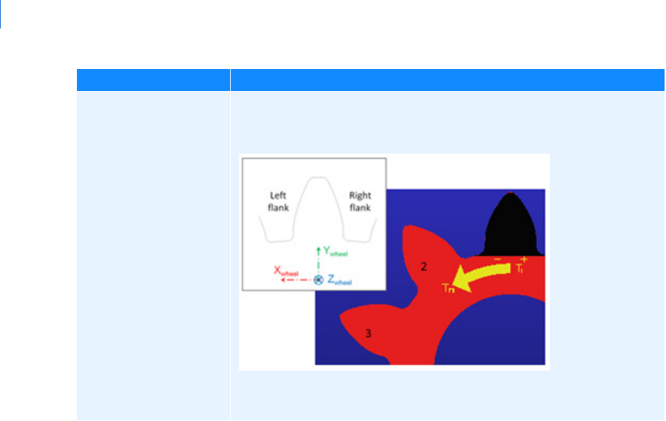
Adams PostProcessor
Gear Contact Pattern
34
Tooth Selected The Contact pattern is available only for the 'Gear_1', that is, first gear of the
gear force definition as shown in below image.
Tooth marked 'Black' is marked as first tooth. Numbering of gear teeth is
marked by Arrow T
1
-T
n
For the option: Do the following:
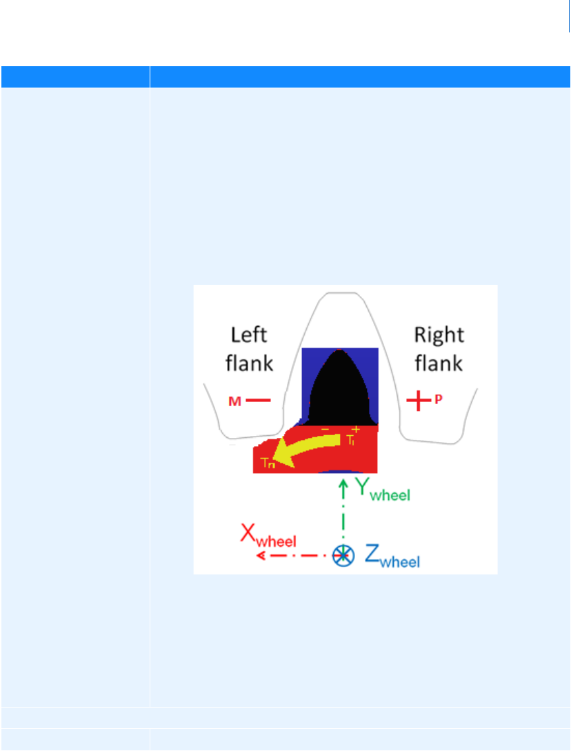
35
Dialog Box - F1 help
Gear Contact Pattern
Flank M(-)
P(+)
Both
Based on sense of rotation:
If Gear_1 (driver or Gear_1 in force definition) rotates
counterclockwise then M(-) flank is in contact
If Gear_1 (driver or Gear_1 in force definition) rotates clockwise then
P(+) flank is in contact
You can also opt to plot Both, if the gear_1 reverses direction of
rotation while simulation and hence both flanks become driving at
least once during simulation.
The flank which is in contact with driven gear and hence drives the
other gear is loaded and the pattern of loading can be plotted by this
feature.
Plot Options
Complete Time Frame Plots of complete Simulation cycle. You can choose selected tooth for plot.
For the option: Do the following:
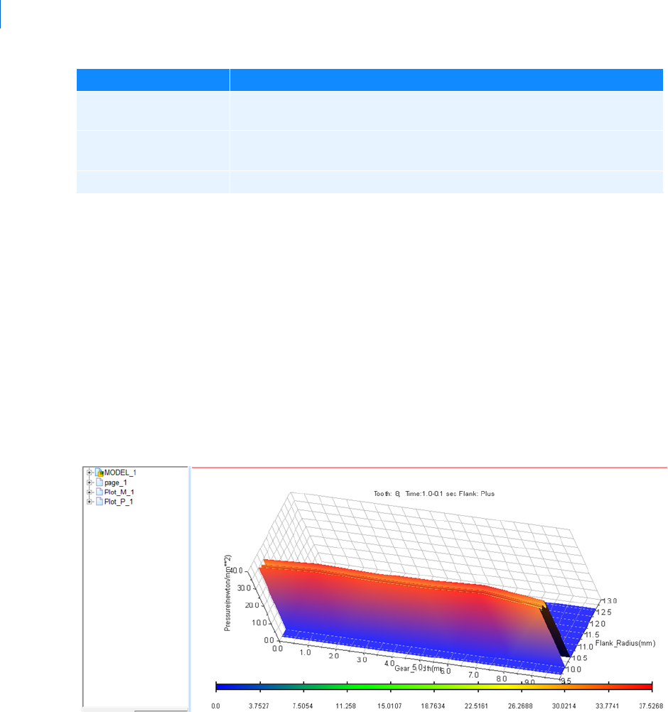
Adams PostProcessor
Gear Contact Pattern
36
Example: Plot of Contact Pattern
Plot options
Flanks = Both : Note two plots in browser (Plot_M_1 and Plot_P_1)
Time Frame = Complete
Tooth Selected = 8
First Axis : Flank Radius (Starting from Contact_Start_Point to Contact_End_Point on tooth)
Second Axis: Gear Width
Third Axis: Pressure
Legend: Mentions tooth number, time frame and flank selected
All teeth Plot of all teeth is generated instead of selected tooth. You can choose time-
frame for which plot is needed.
Select all (All teeth +
complete time frame)
Plot of all teeth with complete time frame will be generated.
Clear Existing Plots Click to clear the existing plots.
For the option: Do the following:
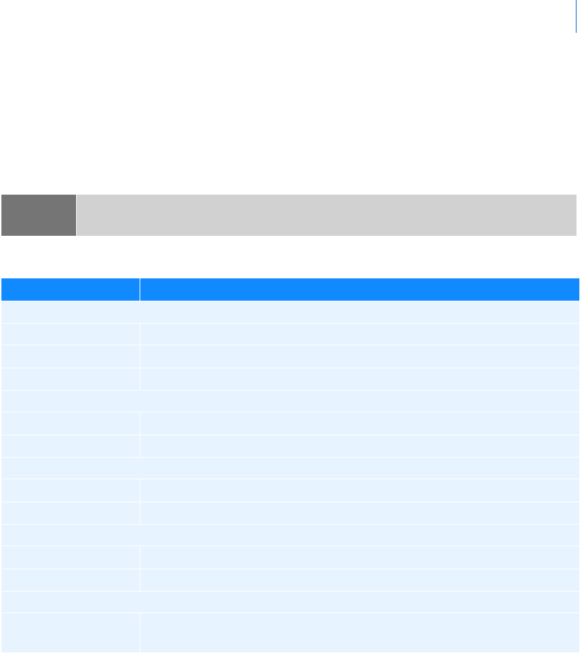
37
Dialog Box - F1 help
Independent Axis Browser
Independent Axis Browser
Plotting dashboard -> Independent axis -> data
Lets you select data other than time for the independent data. The options in the dialog box change
depending on data to which
Source is set in the Dashboard. For example, if the source of the data is Objects, then
the Independent Axis Browser options are those for selecting object data.
Note: The independent axis, by default, is along the x-axis. To change its position, see Setting Up Two-
Dimensional Plot Parameters
.
For the option: Do the following:
If you set Source to Object in the dashboard, the following lists appear:
Object Select the object results whose characteristics you want to plot.
Characteristic Select the characteristic of the selected object that you want to plot.
Component Select one or more components of the characteristic that you want to plot.
If you set Source to Result Set in the dashboard, the following lists appear:
Result Set Select the result set whose components you want to plot. See Result set component.
Component Select one or more components of the result set that you want to plot.
If you set Source to Requests in the dashboard, the following lists appear:
Request Select the Requests whose components you want to plot.
Component Select one or more components of the request that you want to plot.
If you set Source to Clearances in the dashboard, the following lists appear:
Request Select the clearance study whose characteristics you want to plot.
Component Select a component of the clearance study that you want to plot.
If you set Source to System Modes in the dashboard, the following lists appear:
Eigen Select the eigenvalues from a Linear simulation for which you want to create a
scatter plot. You plot the real eigenvalues against the imaginary eigenvalues.
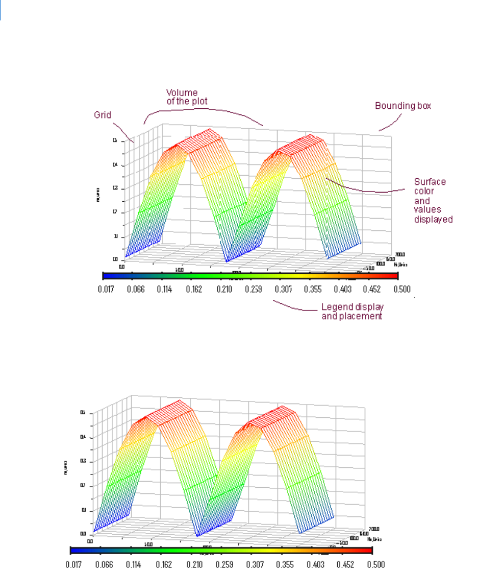
Adams PostProcessor
Picture of bounding box
38
Picture of bounding box
Picture of Plot with Legend
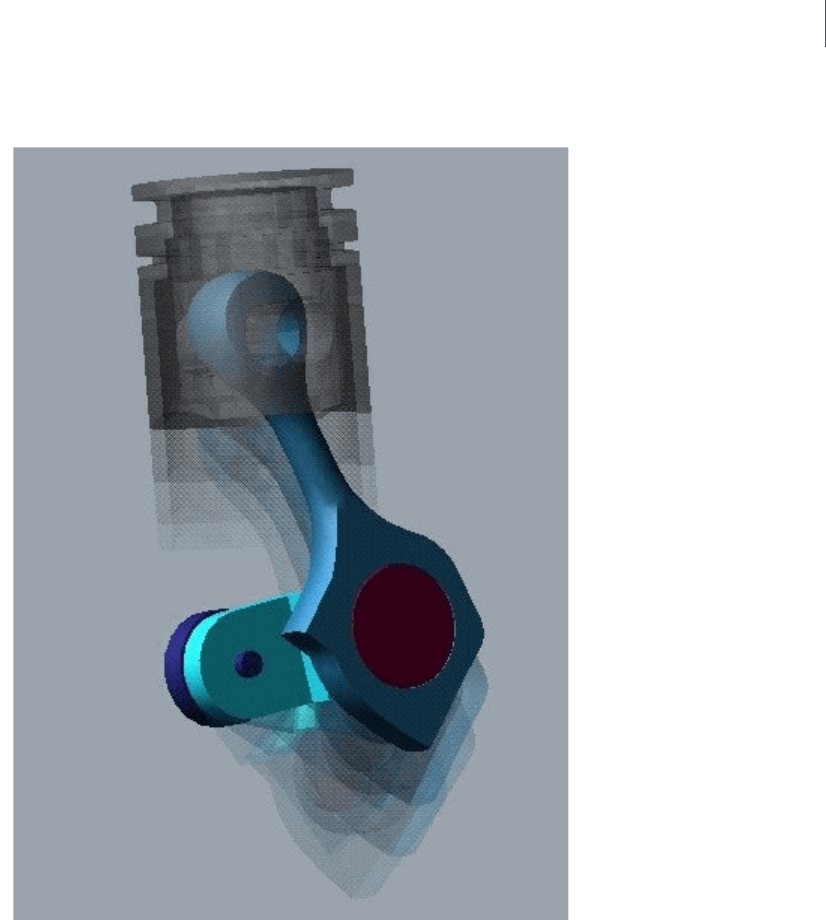
39
Dialog Box - F1 help
Picture of Trailing Frames
Picture of Trailing Frames
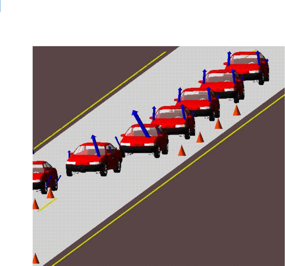
Adams PostProcessor
Picture of superimpose
40
Picture of superimpose
Plotting Dashboard
The dashboard in plotting mode lets you select simulation results to plot. You can build two-dimensional or
three-dimensional plots (Adams Vibration only).
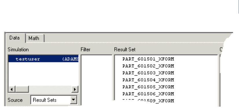
41
Dialog Box - F1 help
Plotting Dashboard - Data
Plotting Dashboard - Data
Plotting dashboard -> Data tab
Lets you create plots of simulation data.
Adams PostProcessor
Plotting Dashboard - Data
42
For the option: Do the following:
For the option: Do the following:
Model/Simulation Select a simulation result to plot. These include Objects, Measures, Requests, result
sets (see
Result set component), system modes, clearance studies, and vibration data
(for Adams Vibration only) and depend on the setting for Source (see below).
The list contains the models or results you have loaded and is set to view object
characteristics by default. If you have three different models loaded, the list of
models would look like the following:
.model_1
.model_2
.model_3
If you are viewing requests, measures, or results sets, the list contains the names
of all the simulations you've imported into Adams PostProcessor. For example, if
you have three different models and two simulations on model_3, then the list
looks like the following:
.model_1.Last_Run
.model_2.Last_Run
.model_3.Last_Run
.model_3.Run_001
Because you see all the simulation results at once, it is easy for you to plot results
between simulation runs and even between simulations from separate models (for
example, plot body acceleration from one model against another model).
Source Set the source of the simulation results. These include objects, measures, requests,
result sets, system modes, and clearance studies. The Model/Simulation list (see
above) changes depending on the selection. Learn more about the
Types of
Simulation Results You Can Plot
.
Filter Select the name of the data you want displayed. For example, you can specify that
Adams PostProcessor only display objects that start with PART_. Type any
wildcards to define the data. For more on wildcards, see
Using Wildcards.
Filter Select the type of data that you want displayed. The objects available to display
depend on the type of results you selected from Source (see above). This is
convenient for large models where the object list could be very long and difficult
to read.
If you set Source to Object, the following lists appear:
Object Select the object results whose characteristics you want to plot.
Characteristic Select the characteristic of the selected object that you want to plot.
Component Select one or more components of the characteristic that you want to plot.
If you set Source to Result Set, the following lists appear:
43
Dialog Box - F1 help
Plotting Dashboard - Data
Result Set Select the result set whose components you want to plot.
Component Select one or more components of the result set that you want to plot.
If you set Source to Requests, the following lists appear:
Request Select the requests whose components you want to plot.
Component Select one or more components of the request that you want to plot.
If you set Source to Clearances, the following lists appear:
Request Select the clearance study whose characteristics you want to plot.
Component Select a component of the clearance study that you want to plot.
If you set Source to System Modes, the following lists appear:
Eigen Select the eigenvalues from a Linear simulation for which you want to create a scatter
plot. You plot the real eigenvalues against the imaginary eigenvalues.
If you set Source to Frequency Response or Transfer Function (Adams Vibration only), the following lists appear:
Input Channels Select the input channels you want to reference.
Use Individually Select one of the following:
Use Individually - Computes and displays a curve for each selected input
channel/output channel pair.
Sum All Input Channels - Computes and displays a curve for each
output channel selected. The curve is the sum of the response for all the
input channels.
Sum Selected Input Channels - Works like Sum All Input Channels,
but only uses the selected inputs.
Output Channels Select the output channels you want to reference.
Phase/Magnitude Select one of the following:
Phase - Plots the phase angle of the response.
Magnitude - Plots the magnitude of the response.
If you set Source to PSD (Adams Vibration only), the following list appears:
Output Channels Select the output channels you want to reference.
If you set Source to Modal Coordinates (Adams Vibration only), the following lists appear:
Input Channels Select the input channels you want to reference.
For the option: Do the following:

Adams PostProcessor
Plotting Dashboard - Data
44
Modal Coordinates By First, select one of the following:
Mode - How the modal coordinate value changes with frequency.
Frequency - What modal coordinates are active at a frequency.
Then, specify the corresponding value below:
Mode - Select the mode whose coordinate value you want to plot.
Frequency - Select the frequencies at which coordinates are to be
plotted.
If you set Source to Modal Participation (Adams Vibration only), the following lists appear:
Input Channels Select the input channels you want to reference.
Output Channels Select the output channels you want to reference.
Modes Select the mode whose participation value you want to plot.
Phase/Magnitude Select one of the following:
Phase - Plots the phase angle of the response.
Magnitude - Plots the magnitude of the response.
Eigen Select the eigenvalues from a Linear simulation for which you want to create a scatter
plot. You plot the real eigenvalues against the imaginary eigenvalues.
The following options are for all types of simulation results:
Surf After selecting the simulation results above, select Surf to quickly scan the results
of your simulation without having to create a large number of plot pages. After
selecting Surf, Adams PostProcessor automatically clears the current plot and
displays the simulation results after you make each selection.
Continue selecting simulation results to plot.
For the option: Do the following:
45
Dialog Box - F1 help
Plotting Dashboard - Math
Plotting Dashboard - Math
Plotting dashboard -> Math tab
Lets you use the Adams View Function Builder to create mathematical expressions that generate curve data as
output. As with any expression in Adams, an expression creating curve data can contain basic math,
trigonometric, and signal-processing functions. For more information on writing expressions, see
Adams View
Function Builder online help
.
Shortcut: To fill the dashboard with current information about a curve, select the curve in the plot window.
Add Curves After selecting the simulation results above, select Add Curves to add curves to
the current plot. You can add as many curves as you'd like. Before selecting the
curves, you can set how you'd like Adams PostProcessor to add them to the plot
using the pull-down menu located below the Add Curves button. You can select:
Add Curves to Current Plot - Adds the curve to the currently selected
plot.
One Curve Per Plot - Creates a new plot on a new page for the curve.
One Plot Per Object, Request, or Result - Creates a new plot for the
curves containing data about a particular object, request, or result. (Not
available for measures.)
Learn more about
Adding Curves to Plots.
Clear Plot Select to clear the current plot of all curves.
Independent Axis Select either:
Time - Use simulation time as the independent axis.
Data - Use other data as the independent axis.
When you select Data, the
Independent Axis Browser appears. Select the desired
data.
Note: The independent axis, by default, is along the x-axis. To change its
position, see
Setting Up Two-Dimensional Plot Parameters.
For the option: Do the following:
Adams PostProcessor
Property Editor - 3D Legend
46
Property Editor - 3D Legend
In treeview -> page -> plot3d -> legend
Lets you edit the legend that appears when you select to have interpolated colors on the surface of your three-
dimensional plot.
Learn how to set up interpolated colors.
Picture of Plot with Legend.
For the option: Do the following:
Curve Name Enter the name of the curve.
Tips on
Entering Object Names in Text Boxes.
Y Expression Change the expression defining the y values for the curve. To access the Function
Builder, right-click the text box, point to Parameterize, and then select Expression
Builder.
Y Units Set the units for the Y expression.
X Expression Change the expression defining the x values for the curve. To access the Function
Builder, right-click the text box, point to Parameterize, and then select Expression
Builder.
X Units Set the units for the X expression.
For the option: Do the following:
For the option: Do the following:
Display Legend Clear to turn off the display of the legend.
Placement Set Placement of the legend to one of the following:
Left
Right
Top
Bottom
Colors Select the number of colors used to display the surface. There can be no more than
255.
Gradients Enter the number of color gradients shown in the legend.
Numeric format options:
47
Dialog Box - F1 help
Property Editor - 3D Plot
Property Editor - 3D Plot
In treeview -> page -> 3D plot
Lets you change the properties of a three-dimensional plot. Learn about changing the surface of the plot.
Property Editor - 3D Surface
In treeview -> page -> 3D plot -> surface_3d
Lets you change the colors and values of the surface of a three-dimensional plot. Learn about changing the
properties of the plot
.
Trai l i n g Z e r o s Select to have Adams PostProcessor display zeros after the numbers in the legend. The
number of zeros depends on the number of decimal places you selected as explained
next.
Decimal Places Enter the number of decimal places to which the numbers in the legend should be
displayed.
Scientific Range Enter the exponential form for scientific notation.
For the option: Do the following:
For the option: Do the following:
Bounding Box Clear to turn off the display of the three-dimensional box surrounding the plot. Picture
of bounding box
.
Grid Clear to turn off the display of the grid.
Graph Volume Enter the x, y, and z aspect ratio of the plot. For example, a volume of 1,1,1 makes the
plot look like a cube, while a volume of 2,1,1 makes the plot twice as long in the x
dimension as it is in the y and z.
Example of Same Data with Different Graph Volumes.
For the option: Do the following:
Skip X/Skip Y Set the x and y increment values you want Adams PostProcessor to skip. Setting it
to 1 for each creates a smooth surface.
Interpolated Colors Select to display the surface of the plot as a range of colors. A legend explaining the
colors and the values they represent appears.
Learn about setting up the legend.
Color Set the single color with which to display the surface.
Number of Colors Enter the number of interpolated colors to be displayed in the plot. There can be no
more than 255.
Adams PostProcessor
Property Editor - Axes
48
Property Editor - Axes
In treeview -> plot -> vaxis/haxis or xaxis/yaxis/zaxis
Lets you edit parameters for horizontal (haxis) and vertical (vaxis) axes of two-dimensional plots and the x-,
y-, and z-axes of three-dimensional plots.
Select a tab:
Format
Labels
Number
Tics
Format Tab
Sets scaling of the axes. By default, Adams PostProcessor automatically scales the axes in a plot based on the
curves.
For the option: Do the following:
Auto Scale Select to have Adams PostProcessor automatically set the minimum and maximum
values, or clear the selection to set the limits manually in the Limits text boxes. By
manually setting minimum and maximum values for the axis, you can zoom in on
different areas of your plot. For example, to view the values between 0 and 10, you can
set the minimum value to 0 and the maximum value to 10. Adams PostProcessor then
only displays the values between these numbers in your plot.
Auto Time Limit Select to have Adams PostProcessor use the current time range as the axis limits, or
clear the selection to set the time limits manually in the Time Limits text boxes.
Note: Setting time limits is only useful when working with the independent
(horizontal) axis.
Tip: For linear- and dB-scaled axes, enter lower and upper limits. For logar-
scaled axes, enter log base 10 for lower and upper limits. (See Scale below.)
Scale Set to the type of scaling. By default, Adams PostProcessor displays the axis values
linearly, starting at 0. You can also change the scaling to:
Logarithmic - Scales the axis values so that each power of 10 is separated by
the same distance. For example, the values 1, 10, 100, 1000, and 10,000 are
equally spaced.
Decibel (dB) - Displays 20 * log
10
(value) for each value.
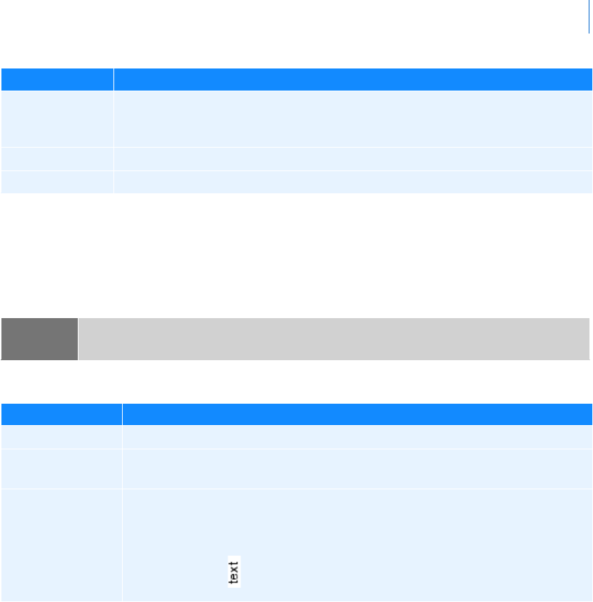
49
Dialog Box - F1 help
Property Editor - Axes
Labels Tab
Sets label parameters. By default, Adams PostProcessor displays a label next to an axis to help identify the
values in the axis. The label identifies the unit of measurement in the axis. You can change the text of the
label, its placement, font size, and color.
Placement Set to where you want to place the axis. The options available depend on whether you
are modifying the horizontal or vertical axis. You can place an axis on the right or left
or at the top or bottom.
Offset Set how far from the border of the plot you want to display the axis.
Color Select the color for the axis.
For the option: Do the following:
Note: You can also modify the label text using the instructions in Adding Notes and Modifying Text, which
enables you to create multi-line labels.
For the option: Do the following:
Label Enter the text for the label.
Font Size Enter a font size. The font size you can enter depends on the type of font you
selected.
Horizontal/Vertical Set the orientation of the label, either:
Horizontal - text
Vertical -
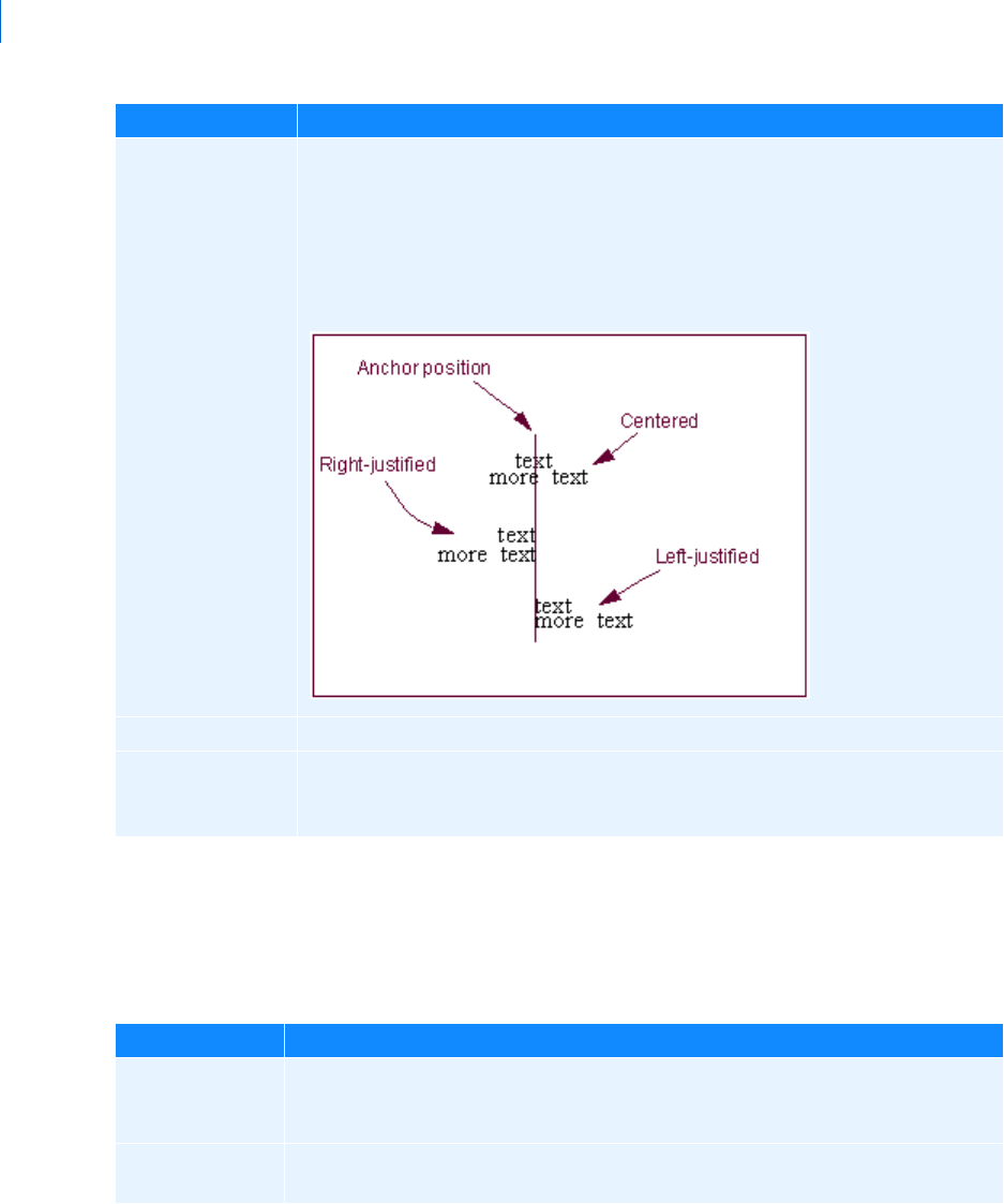
Adams PostProcessor
Property Editor - Axes
50
Numbers Tab
Sets the display of numeric values for an axis. By default, Adams PostProcessor displays numeric values for an
axis at each major increment. You can change the way in which Adams PostProcessor displays the values, such
as the number of decimal places displayed and whether or not Adams PostProcessor uses scientific notation.
Left/Center/Right Select how you want the label to be aligned relative to its anchor position, which is
the center of the text. See the figure below. You can select:
Left - Left-justifies the text from the anchor position.
Center - Centered the text on its anchor position.
Right - Right-justifies the text from the anchor position.
Color Select the color for the axis.
Auto Place/Offset/
No Choice
Select to have Adams PostProcessor place the text, or clear the selection of Auto Place
and, in the Offset text box, enter an offset value to define the distance the label is
offset from the border of the plot.
For the option: Do the following:
Tr a i l i n g Ze r o s Select to have Adams PostProcessor display zeros after the numbers in the axis. The
number of zeros depends on the number of decimal places you selected as explained
next.
Decimal Places Enter the number of decimal places to which the numbers in the axes should be
displayed.
For the option: Do the following:
51
Dialog Box - F1 help
Property Editor - Column
Tics Tab
By default, Adams PostProcessor displays short lines, called tic marks, at regular intervals across the axis. The
tic marks help to define the scale of the axis. Adams PostProcessor displays the major tic marks at every unit
value and the minor tic marks halfway between the major tic marks.
For major tic marks, you can set the spacing by setting:
Increments - Specifies intervals across the axis, such as at every unit value, every second unit value,
and so on, at which tic marks should appear.
Divisions - Divides the axis evenly into a number of segments and places a tic mark at every division.
For minor tic marks, you can set how many minor tic marks appear between each major tic mark.
Property Editor - Column
In treeview -> page -> plot set as table -> curve
Lets you change the properties of the independent data column of a plot set to be viewed as a table.
Learn about setting the general properties of the table.
Scientific Range Enter the exponential form for scientific notation.
Font Size Enter a font size. The font size you can enter depends on the type of font you selected.
Color Select the color for the numbers.
For the option: Do the following:
Auto Divisions To turn off automatic divisions, clear the selection of Auto Divisions and select how
you want the major tic marks spaced from the pull-down menu. Enter the number of
increments or divisions in the text box.
Minor Divisions Enter the number of divisions between each major tic mark. The number of divisions
sets the number of minor tic marks. For example, if you set the number of divisions to
two, Adams PostProcessor places one minor tic mark between each major tic mark.
Color Select the color for the numbers.
For the option: Do the following:
Note: Even though you toggled a plot to display as a table, the treeview still lists it as a plot and all
of its columns as curves.
Adams PostProcessor
Property Editor - Curve
52
Property Editor - Curve
In treeview -> plot -> curve
Lets you edit the attributes of a curve on a plot. You can also set defaults for how Adams PostProcessor creates
curves, as explained in
PPT Preferences - Curves.
For the option: Do the following:
Legend Change the legend text that appears above the column. If you set the columns so they
are brief (for example, Column 1 instead of LEFT FRONT CONTACT MATCH
MOTION_Z), Adams PostProcessor changes the text that appears in the row
containing the legend text. Learn about
Changing Table Properties. Examples of Complete
and Brief Headers for Tables
.
Tr a i l i n g ze r o s Select to have Adams PostProcessor display zeros after the numbers in the axis. The
number of zeros depends on the number of decimal places you selected as explained
next.
Decimal places Enter the number of decimal places to which the numbers in the axes should be
displayed.
Scientific range Enter the exponential form for scientific notation.
Note: In addition to setting a curve's properties, you can edit the data in the curves. Learn about
Performing Calculations on Curves.
53
Dialog Box - F1 help
Property Editor - Curve
For the option: Do the following:
Legend Enter the text to appear in the legend associated with this curve. Adams
PostProcessor displays the legend with a short line segment illustrating the
color and line style of the curve. If you updated your plots, Adams
PostProcessor creates a second legend, called the simulation legend. You
modify the simulation legend text separately. For more information on
modifying legends, see
Modifying Legend Properties. For more information on
the types of legends, see
Updating Plot Data.
Tip: You may want to expand the width of the Property Editor so you
have more space for entering the legend text. To expand the
property editor, point to its right border. When the cursor
changes to a double-sided arrow, drag the cursor to increase the
property editor's size.
Line Color Select the Line Color for the text and curve.
Line Style/Line Weight Select the type of line style and weight for the curve. The weight values
range from 1 to 5 screen pixels. Set the line style to None so that Adams
PostProcessor does not display the curve line. If you selected to display
symbols along the curves, the symbols still appear when you turn off the
curve line.
Symbol/Symbol increment Select the type of symbol that you want at data points along the curve and
select how often you would like the symbol to be displayed along the curve.
Hotpoints Select to turn on Hotpoints that let you manually edit the data points in the
curve. You can also control how you edit the hotpoints, only vertically or
only horizontally, so you have greater control. For more on hotpoints and
manually editing curves, see
Manually Changing Data Point Values.
Select one of the following:
No - To have no hotpoints displayed.
Yes - Turn on hotpoints, to allow the editing of the data points in
any direction.
Horizontal - Turn on hotpoints, but only allows the editing of the
data points in the horizontal direction.
Vertical - Turn on hotpoints, but only allows the editing of the
data points in the vertical direction.
Note: You can use the Hotpoints tool on the Curve Edit toolbar
to override this setting. See
Displaying the Curve Edit Toolbar.

Adams PostProcessor
Property Editor - Flexible Body
54
Property Editor - Flexible Body
In treeview -> page -> model-> flexible body
Lets you change the display and animation properties for a flexible body.
Display Attrs tab
For more on the options in the Display Atts tab, see the help for the Property Editor - Modeling Object.
55
Dialog Box - F1 help
Property Editor - Flexible Body
Flex Props tab
For the option: Do the following:
Plot Type Set to the type of plot (Contour, Vector, or Both). Learn more about flexible body
plots with
Animating Deformations, Modal Forces, and Stress/Strain.
Scale Enter a value by which to scale the deformations. Set a large scale to exaggerate the
deformations.
Note: By default, animations containing flexible bodies display the nodal
deformations for the bodies at each frame of the animation. To display
these nodal deformations, Adams PostProcessor computes a cache of
information before displaying the animation. The generation of this cache
can cause a delay in the initial display of the animation. You can avoid the
caching delay by turning off the nodal deformations and displaying the
flexible bodies in their undeformed shapes only. To turn off the nodal
deformations, set the scale to 0, which treats the flexible body like a rigid
body, showing no physical deformations. You can still display the
Contour
plots
and Vector plots. Note that these settings only apply to animations and
will not affect the simulation of the specified bodies.
Adams PostProcessor
Property Editor - Flexible Body
56
Render Set the flexible body rendering to:
Flat - Renders flexible bodies more simply, with flat edges. Uses face normals
to produce a faceted rendition of the body. Also, the normals are calculated
for the undeformed body and are reused when showing its deformed shaped.
This is the fastest of the rendering options but can produce some incorrect
light intensities for bodies with large nodal deformations.
Smooth - Renders the flexible body with smooth, rounded edges, appropriate
for presentations, but slows down the animation. It uses vertex normals to
produce the smooth rendition of the body and also uses normals calculated
for the undeformed body.
Precision - Renders the highest quality image for the flexible body at a cost of
decreased drawing speed for the body. It uses vertex normals to produce a
smooth rendition of the body. When the body is displayed in a deformed
context, such as when contained in an animation, the normals are calculated
for each deformed shape. This option produces the most accurate shading for
each body but is slower than the other options. We recommend that this
option only be used when producing movie files or hardcopy images for
presentation purposes.
Datum Node Set the datum node to which you want deformation color changes to be relative.
Adams PostProcessor considers the deformation to be relative to the origin of the
flexible body (its local body reference frame (LBRF) or coordinate system) by default.
For example, if you were modeling a cantilever beam, you could specify that
deformations should be relative to the clamped end.
Tip: To select a node from the screen, right-click the Datum Node text box, and
then select Pick Flexbody Node. Select the node from the screen. The node
number appears in the Datum Node text box.
For the option: Do the following:
57
Dialog Box - F1 help
Property Editor - Legend
Property Editor - Legend
In treeview -> plot -> legend_object
Lets you change the placement and border of legends on your plots. There are two types of legends in Adams
PostProcessor:
Curve legend text that describes the data that each curve on the plot represents.
If you update your plot data, as explained in Updating Plot Data, Adams PostProcessor creates a second
legend, called the simulation legend. The simulation legend contains groups of text that describe the
data in a specific simulation.
This does not let you change the text of legends. Learn about
Setting Curve Properties.
You also cannot change the legend when a plot is displayed as a table. Learn about
Displaying Plots as Tables.
Mode Filter Select a filter type, as explained below. By default, all enabled modes are used to
generate nodal displacements for each flexible body during animations. To increase
animation performance, Adams PostProcessor has three filters that let you remove
graphically insignificant modes for animations. A mode that is filtered out is excluded
from the modal superposition and any contribution to the deformation of the body is
ignored. Note that these modes are not filtered out for numeric operations, such as
signal processing or xy plotting.
None - Includes all modes for computing the graphics display.
Frequency - Excludes any mode that is activated above the specified
frequency.
Min Displacement - Excludes any mode that does not contribute the
minimum displacement specified for at least one vertex of the flexible body.
For example, if you are viewing the animation of a vehicle driving down the
road, it is unlikely that you would be able to see deformations of 0.5 mm or
less. Therefore, if you set a mode filter value of 0.5, any mode that contributes
less then 0.5 is considered insignificant and is ignored for animations. This
calculation is performed at each frame of the animation, allowing the set of
significant modes to change throughout the simulation event.
Percentage - Determines the maximum displacement contributed by all
modes, and excludes any mode that doesn't contribute displacement of one
vertex at least as significant as a percentage of the maximum. For example,
setting the percentage filter at 15% excludes any mode not contributing at
least 15% of the most dominant mode. This calculation is performed for each
frame of the animation, therefore, allowing the set of significant modes to
change throughout the simulation event.
For the option: Do the following:
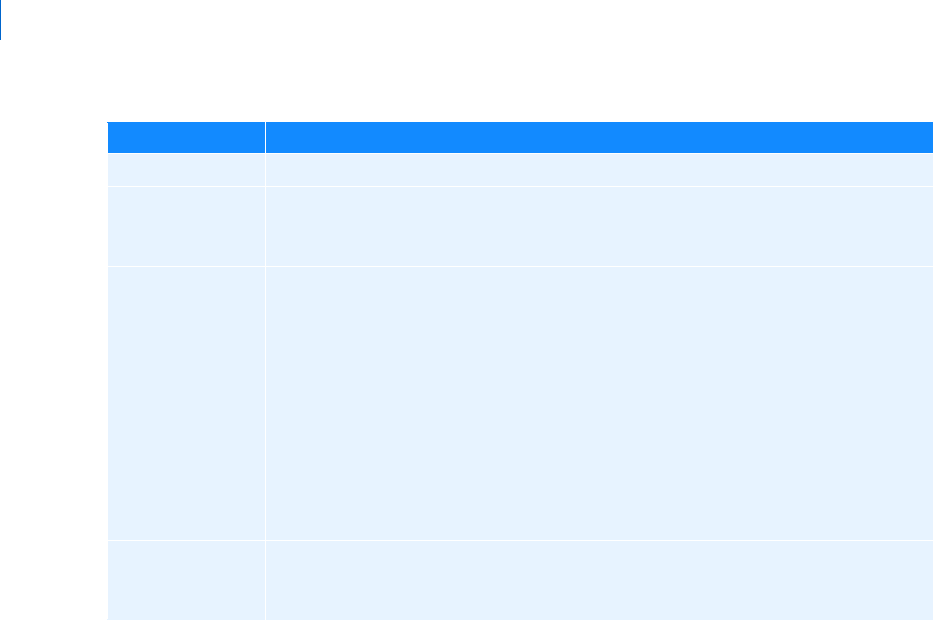
Adams PostProcessor
Property Editor - Modeling Object
58
Property Editor - Modeling Object
In treeview -> page -> model -> object
Lets you edit the display properties for a modeling objects, such as a parts, geometry, or Markers. By default,
all objects inherit the display options that you specify for their parents. For example, geometry and markers
inherit the options set for the part to which they belong. Therefore, if you turn off the display of a part, you
no longer see its geometry or markers. You can override the inheritance, however, by selecting a particular
geometry and turning on its display, as shown below.
For the option: Do the following:
Display Legend Select to turn on the display of legend.
Legend
Background
Clear its selection if you want the legend to be transparent. Any plot information
behind the legend shows through. When you select Legend Background, the legend
is opaque and covers any information behind it.
Placement Set to one of the following:
Top Right
Top Left
Bottom Left
Bottom Right
Axis - Places the legend text for each legend on the appropriate dependent
axis.
User-placed - Sets the legend so you can move it to any position, as explained
in
Moving Text.
Legend Borderline Clear the selection if you do not want a borderline around the legend. If you do want
a borderline, keep Legend Borderline selected and then select a line color, line weight,
and line style for the borderline.
59
Dialog Box - F1 help
Property Editor - Modeling Object
Learn about:
Changing display options for spring dampers
Setting Animation Display Options for Flexible Bodies
Here display is set to on for parent part, and
all its children inherit the display setting.
But here, display is set to off for the parent
part but on for one geometry in part, so its
setting overrides the parent setting.
For the option: Do the following:
Visibility Set Visibility to whether or not you want to turn on the display of the selected object.
You can select:
On - Turns on the display of the object.
Off - Turns off the display of the object.
Inherit - Lets the object simply inherit the display settings from its parent.
No Choice - Does not change the current settings. Lets you make changes to
other display options without affecting the visibility of the objects.
Name Visibility Select if you want the names of objects displayed. Refer to Visibility above for an
explanation of the choices.
Adams PostProcessor
Property Editor - Note, Title, or Subtitle
60
Property Editor - Note, Title, or Subtitle
In treeview -> plot -> title/note/subtitle
Lets you edit the text of notes, titles, and subtitles.
Color Select the color for the object.
Icon Size Enter the size you want for the Screen icons of the object or select the amount by which
you want to scale the icons. The scale factor is relative to the current size set. A scale
factor of 1.0 keeps the icons the same size. A scale factor less than 1.0 reduces the size
of the icons, and a scale factor greater than 1.0 increases the size of the icons. Note
that these changes take precedence over the size you specify globally for the modeling
database.
Tr a n s Set how transparent the object is. The higher the value, the more transparent the
object is, allowing other objects to show through. The lower the value, the more
opaque the object is, covering other objects. (Not available for spring-dampers.)
Tip: Setting the transparency of objects can have a negative impact on rendering
performance if you are using a graphics card without hardware acceleration
for OpenGL. Instead of setting an object's transparency, consider setting
the object's render mode to wireframe.
For the option: Do the following:
For the option: Do the following:
Text a r e a Enter or change the text in the text area. You can enter multiple lines of text.
Font Size Enter a font size. The font size you can enter depends on the type of font you
selected.
Horizontal/Vertical Set the orientation of the text, either:
Horizontal - text
Vertical -
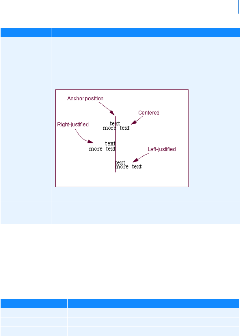
61
Dialog Box - F1 help
Property Editor - Page
Property Editor - Page
In treeview -> page
Lets you display headers and footers on all pages. Each header and footer can have three items of information
(left, center, and right). Each item on the header footer can be a bitmapped image (.jpg, .xpm, or .bmp) or
text.
You can also set up default headers and footers to appear on all pages as explained in
PPT Preferences - Page.
Left/Center/Right Select how you want the text to be aligned relative to its anchor position, which is
the center of the text. See the figure below. You can select:
Left - Left-justifies the text from the anchor position.
Center - Centered the text on its anchor position.
Right - Right-justifies the text from the anchor position.
Color Select the color for the text.
Auto Position Select Auto Position to have Adams PostProcessor automatically set the location of
the text or clear the selection of Auto Position and enter a location for the text in
the text boxes that appear.
For the option: Do the following:
For the option: Do the following:
Header/Footer/None Select to set up a header, footer, or neither.
Left/Center/Right Select the item of information (left, center, or right) that you are setting up.
Source Choose either Text or Image.
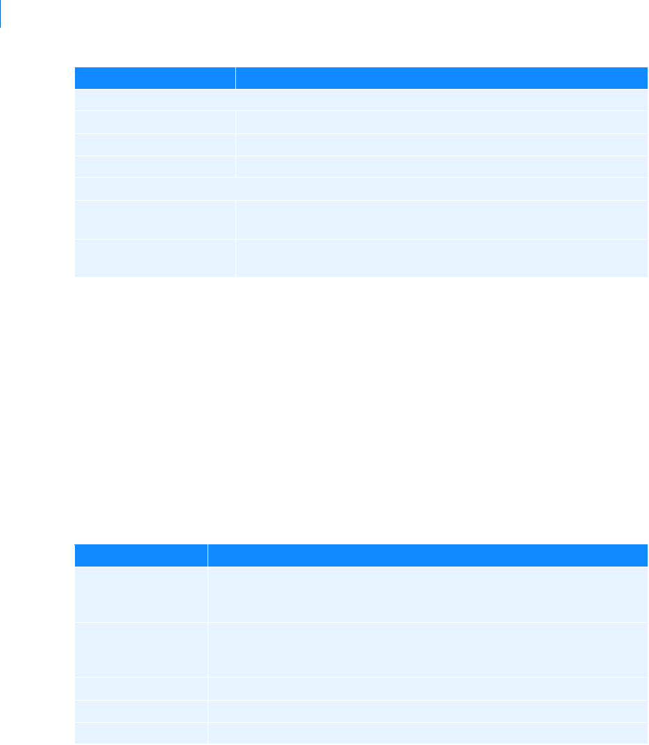
Adams PostProcessor
Property Editor - Plot
62
Property Editor - Plot
In treeview -> plot
Lets you set plot parameters. See Listing of Plot Parameters.
Select a tab:
General
Border
Grid/2nd Grid
General Tab
Sets plot parameters for title, subtitle, and axis placement.
If you set Source to Text, Adams PostProcessor displays the following options:
Te xt Enter the text you want to appear in the header or footer.
Font Size Enter the font size.
Color Select a color from the pull-down menu.
If you set Source to Image, Adams PostProcessor displays the following options:
Image Enter the image you want to appear in the header or footer. The image can
be a .jpg, .xpm, or .bmp.
Height Enter the height at which you want the image displayed. Adams
PostProcessor automatically displays the image as 50 pixels high.
For the option: Do the following:
For the option: Do the following:
Auto Title/Title Select to have Adams PostProcessor automatically generate titles or clear the
selection, and in the Title box, enter the text for the title. The title can only be a
single line of text.
Auto Subtitle/Subtitle Select to have Adams PostProcessor automatically generate subtitles or clear the
selection of Auto Title or Auto Subtitle, and in the Subtitle box, enter the text
for the subtitle. The subtitle can only be a single line of text.
Analysis Select to have the analysis name appear on the plot.
Date Stamp Select to have the date on which the analysis was generated appear on the plot.
Legend Select to add legend text. Learn about Modifying Legend Properties.
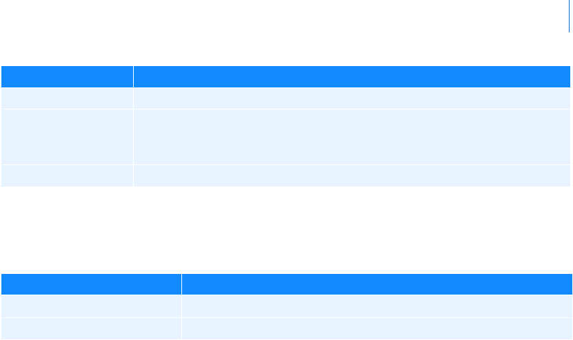
63
Dialog Box - F1 help
Property Editor - Plot
Border Tab
Sets border parameters.
Zero Line Select to create a line at the position 0,0.
Dep. Axis Set where you want the dependent axis of data to appear by selecting either
Horizontal (along the x-axis) or Ve rtic al (along the y-axis). Note that you can
only change the orientation if there are no curves on the plot.
Table Select to display plot in tabular form. Learn about Displaying Plots as Tables.
For the option: Do the following:
Line Color Select a Line Color for the border.
Line Style Select the type of line style for the border.
For the option: Do the following:
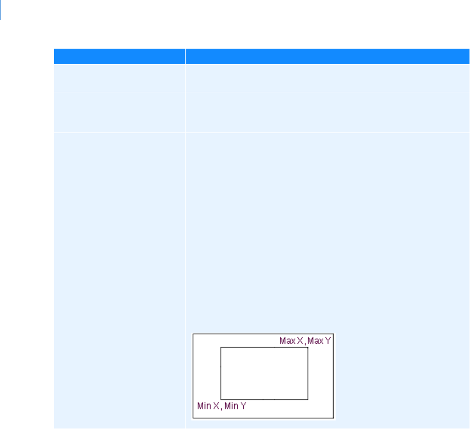
Adams PostProcessor
Property Editor - Plot
64
Grid/2nd Grid Tabs
Sets grid parameters. Adams PostProcessor displays grids on a plot to provide visual guides for inspecting
curves. You can have primary and secondary grid lines. Primary grid lines appear at all major unit sections.
Secondary grid lines appear at specified intervals between the primary grid lines. If you turn off the primary
grid lines, Adams PostProcessor also turns off the secondary grid lines.
Line Weight Select the weight for the border. The weight values range from 1 to 5
screen pixels.
Auto Fit Border Select to center the plot in the viewport (see Viewports) and keep it
centered even when you make modifications to its layout, or clear to set
your own margins for the plot.
Min X, Max X, Min Y, Max Y To set your own margins for the plot, after clearing the selection of Auto
Fit Border, and then enter the minimum and maximum values for the
margin in the x and y directions in pixels. See the figure below for
assistance.
Min X - Sets the space from the left edge of the window to the
left edge of the plot.
Max X - Sets the width of the plot. It includes the left margin
that Min X defines.
Min Y - Sets the size of the space from the bottom edge of the
window to the bottom edge of the plot.
Max Y - Sets the height of the plot including the bottom margin
that Min Y defines.
Minimum and Maximum Values for Borders
For the option: Do the following:
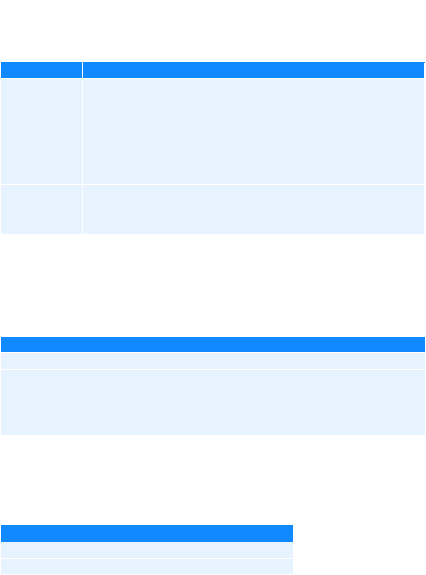
65
Dialog Box - F1 help
Property Editor - Reports
Property Editor - Reports
In treeview -> page -> report
Lets you change the properties of Reports. After you import a report, you can change the source file associated
with the report and the size of the font used to display the report.
Property Editor - Scatter
In treeview -> page -> plot -> scatter
Lets you change the properties of scatter plot of eigenvalues from a Linear simulation.
For the option: Do the following:
Visible Clear to turn off the display of the grid.
Line
Count/Increment/
No Choice
(Primary grid only)
Set the number of lines by selecting either:
Line Count and entering the number of lines in the grid.
Increment and entering the amount of space between each grid line in the x
and y directions. Enter the values in length units.
Line Color Select a Line Color for the grid.
Line Style Select a line style for the grid.
Line Width Select a weight for the grid. The weight values range from 1 to 5 screen pixels.
For the option: Do the following:
File Name Change the source file for report.
Font Size Enter the size for logical font size 3 (HTML logical font point sizes are from 1 to 7;
they define font point sizes relative to one another; not in absolute values). All other
font point sizes are scaled according to the value you enter for font size 3. For example,
if you set the report font point size to 10 points, then logical font size 3 is 10; font size
2 is 8 points; and so on.
For the option: Do the following:
Color Select the color for the symbols.
Symbol Select the symbol used to display the scatter plot.
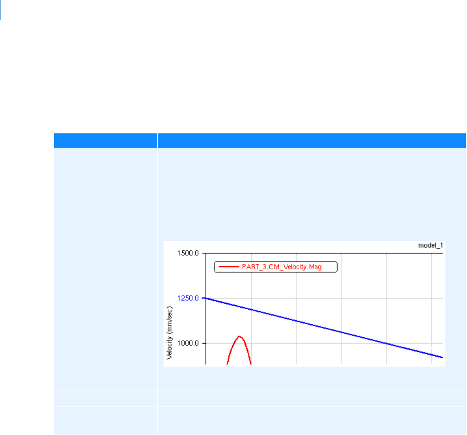
Adams PostProcessor
Property Editor - Spec Line
66
Property Editor - Spec Line
In treeview -> plot -> spec_line
Lets you edit the properties of spec lines.
Learn more about
Adding Spec Lines.
Property Editor - Spring Damper
In treeview -> page -> model -> spring_damper
Lets you edit the display of a spring damper. The tab Disp Attrs is explained below. For information on the
Object Props tab, see
Property Editor - Modeling Object.
A spring damper is a graphic representation of a spring and damper drawn between two
Markers. The spring
damper stretches along the axis created by its I and J markers. The figure below illustrates the display options
you can set.
For the option: Do the following:
X Value/Y Value For a horizontal spec line, enter only a y value.
For a vertical spec line, enter only an x value.
For a diagonal spec line, enter both an x and y values.
For example, entering both x and y values, provides the following diagonal spec
line:
Line Color Select the Line Color for the text.
Line Style/Line Weight Select the type of line style and weight for the spec line. The weight values range
from 1 to 5 screen pixels.

67
Dialog Box - F1 help
Property Editor - Table
Property Editor - Table
In treeview -> page -> plot set as table
Lets you change the properties of a plot in tabular format.
Select a tab:
General
Independent Column
For the option: Do the following:
Coil Count Enter the number of coils drawn in the spring.
Spring Diameter Enter the diameter of the spring.
Damper Diameter: I and J Enter the diameters of the dampers at the I and J markers.
Tip Length: I and J Enter the distances between the ends of the dampers and the I and J markers.
Cup Length: I and J Specify the length of the damper cups in a spring-damper graphic. The first
value defines the length of the cup at I marker. Adams PostProcessor measures
the length from the bottom of the cup to its top along the line that I and J
define. The second value defines the length of the cup at J. Adams View
measures the length from the bottom of the cup to the top along the line that
I and J define.
Note: Even though you toggled a plot to display as a table, the Treeview still lists it as a plot and all of
its columns as curves.
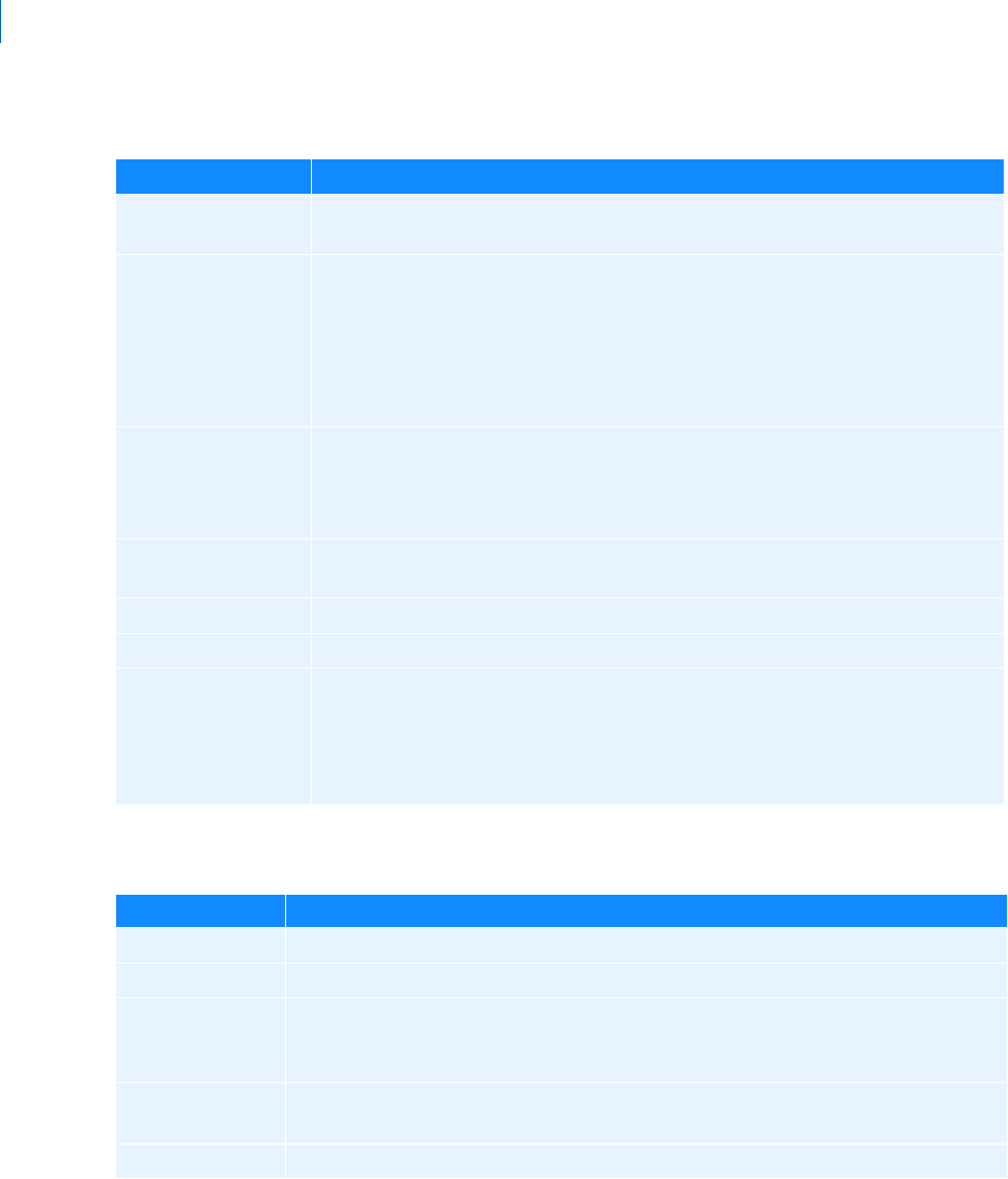
Adams PostProcessor
Property Editor - Table
68
General Tab
Independent Column
For the option: Do the following:
Auto Header Select to have Adams PostProcessor automatically generate a header for the report.
Clear to create your own header.
Header If you selected to create your own header,enter the text for the title and subtitle.
The title and subtitle can only be a single line of text.
Tip: You may want to expand the width of the property editor so you have
more space for entering the text. To expand the property editor, point to
the sash on its right border. When the cursor changes to a double-sided
arrow, drag the cursor to increase the property editor's size.
Limits Specify the start and end for values in the table (start and end are specified as values
in the independent data column). Note that these limits are the axis limits on the
independent axis. When you toggle back to a plot, they will be in effect on that
axis.
Row inc Set the increment for the data to be included. For example, select 1 to include every
data point; select 5 to include every 5th data point.
Font Size Enter a font size. The font type is always Helvetica.
Alignment of Values Set to where you want to position the values in the columns.
Legend Select to add legend text and set the column legends so they are brief (for example,
Column 1 instead of LEFT FRONT CONTACT MATCH MOTION_Z).
Adams PostProcessor adds a new row under the title containing the legend text.
The legend text maps column names to data names.
Examples of Complete and Brief
Headers for Tables. Learn about changing the legend text
.
For the option: Do the following:
On Clear its selection to remove the display of the independent column.
Legend Enter the text in the text box to change the legend for the independent column.
Tr a i l i n g Ze r o s Select to have Adams PostProcessor display zeros after the numbers in the table. The
number of zeros depends on the number of decimal places you selected as explained
next.
Decimal Places Enter the number of decimal places to which the numbers in the table should be
displayed.
Scientific Range Enter the exponential form for scientific notation.
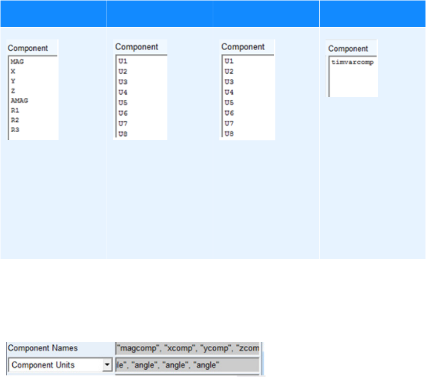
Appendix
About the "REQSAVE_COMPATIBILITY" analysis
Requests in Adams View sessions create results components by default in Adams PostProcessor
These components names are generic and user may want to override it using specific names for customized
requests, for example, bearing_stiffness_x, bearing_stiffness_y and so on. User can change these default
names by using 'component_names' fields in request dialog box as below:
(Default component_name 'MAG' is replaced by 'magcomp' as seen next)
The names could be confusing to another/same user who is reviewing the request in Adams PostProcessor.
Hence, there is a provision to create/discard dummy analysis retaining default names.
Using Type and Markers Using Subroutine
Using Function
Expressions
Using Variables
Eight components:
magnitude and x-y-z
components, each for
translational and
rotational elements
Typ i cal ly ge n era t ed f o r
displacement, velocity,
acceleration and force
Eight components based
on type of request (could
be GFOSUB, REQSUB,
MOTSUB and so on.)
Hence, names are
generic like U1, U2 and
so on.
Eight components based
on type of request (could
be any adams function
like JOINT, AX(), DM()
and so on.)
Hence, names are
generic like U1, U2 and
so on.
One component created
per request
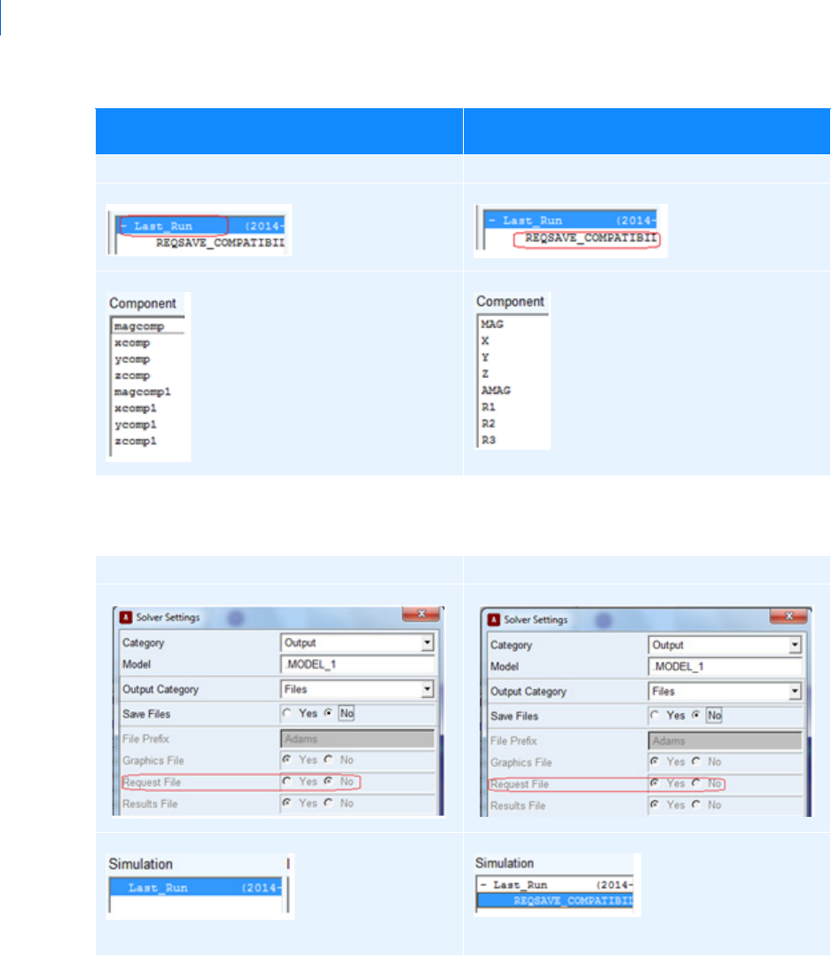
Adams PostProcessor
About the "REQSAVE_COMPATIBILITY" analysis
78
This dummy analysis can be turned off by setting Request file flag in the solver settings as shown below:
Please note that while REQSAVE_COMPATIBILITY is being turned ON/OFF, the choice is combined with
save_files → yes/no.
Hence, for making request_file flag (and hence REQSAVE_COMPATIBILITY) ON/OFF:
User created request with customized component
names
Dummy analysis saved by Adams retaining
original default names
Analysis_Name: LAST_RUN (or other) Analysis_Name: REQSAVE_COMPATIBILITY
No REQSAVE_COMPATIBILITY required REQSAVE_COMPATIBILITY required
No REQSAVE_COMPATIBILITY created
REQSAVE_COMPATIBILITY created
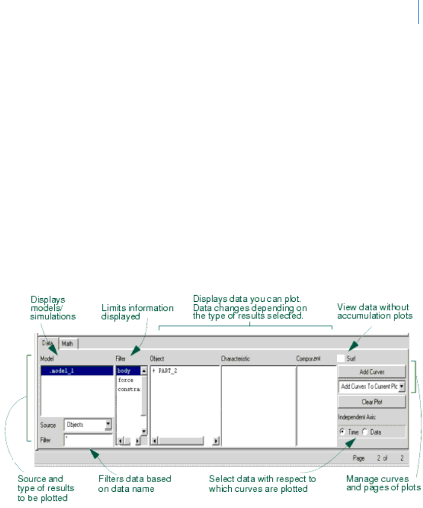
79
Appendix
Contour plots
1. User needs to first set 'Save_file' to 'YES' to make choice 'Request_File' enabled, change the option
to YES/NO as required
2. Next; set the 'Save_File' to YES/NO as per requirement (setting it to YES will save analysis files too,
that is, .gra, .res, .req with internal solver)
Contour plots
Contour plots graphically display scalar data on the elements of flexible bodies and FE Parts at each output
step. Different quantities are available and displayed in the option menu for the different modeling objects
supporting contour plots: flexible bodies (linear and nonlinear types) and FE Parts. For more information
about contour plotting for linear flexible bodies see Adding Contour or Vector Plotting, for nonlinear flexible
bodies see Reviewing Results and for the FE Part see Animation Capabilities.
See also Vector plots.
Dashboard
Provides functions for controlling animations or plotting results. It appears at the bottom of Adams
PostProcessor.
Entering Object Names in Text Boxes
To enter object names in text boxes, you can do either of the following:
Enter the object name directly in the text box.
Clear the text box and then double-click to open the Database Navigator.
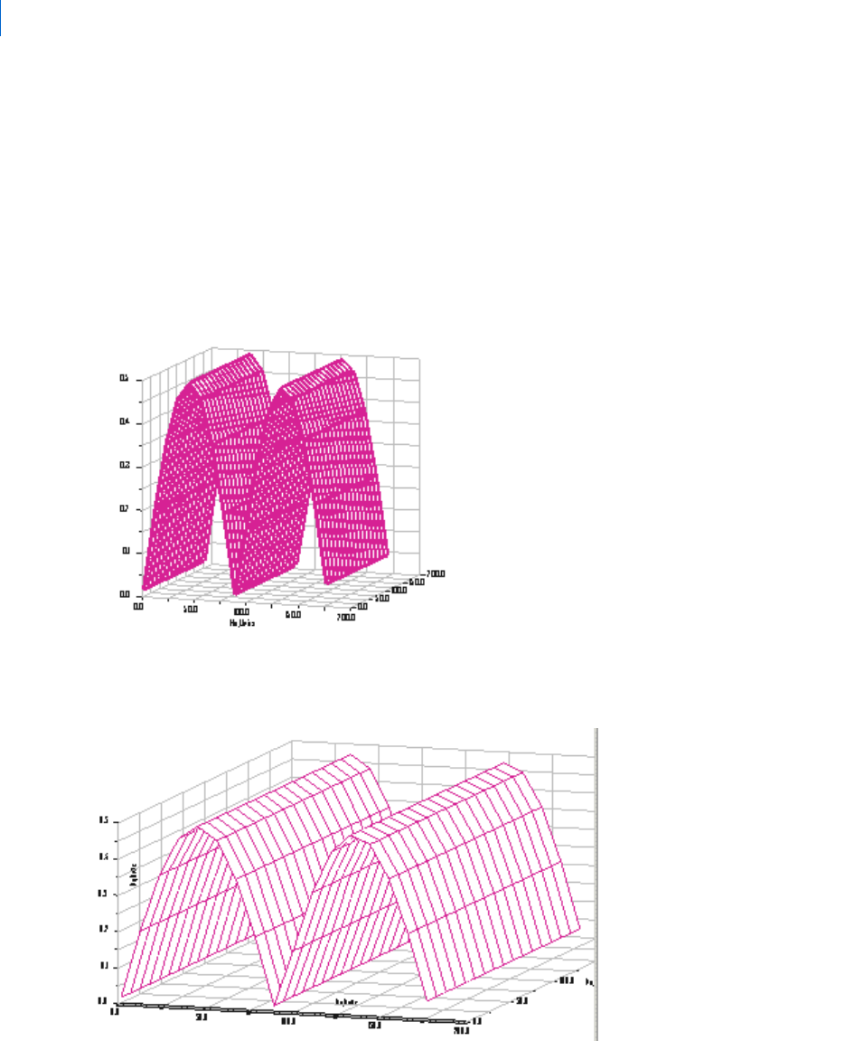
Adams PostProcessor
Example of Same Data with Different Graph Volumes
80
Right-click to either:
• Pick an object shown on the screen.
• Browse a complete list of available objects.
• Choose from a product-generated list of guesses.
Example of Same Data with Different Graph Volumes
Graph Volume 1,1,1
Graph Volume 2,3,1
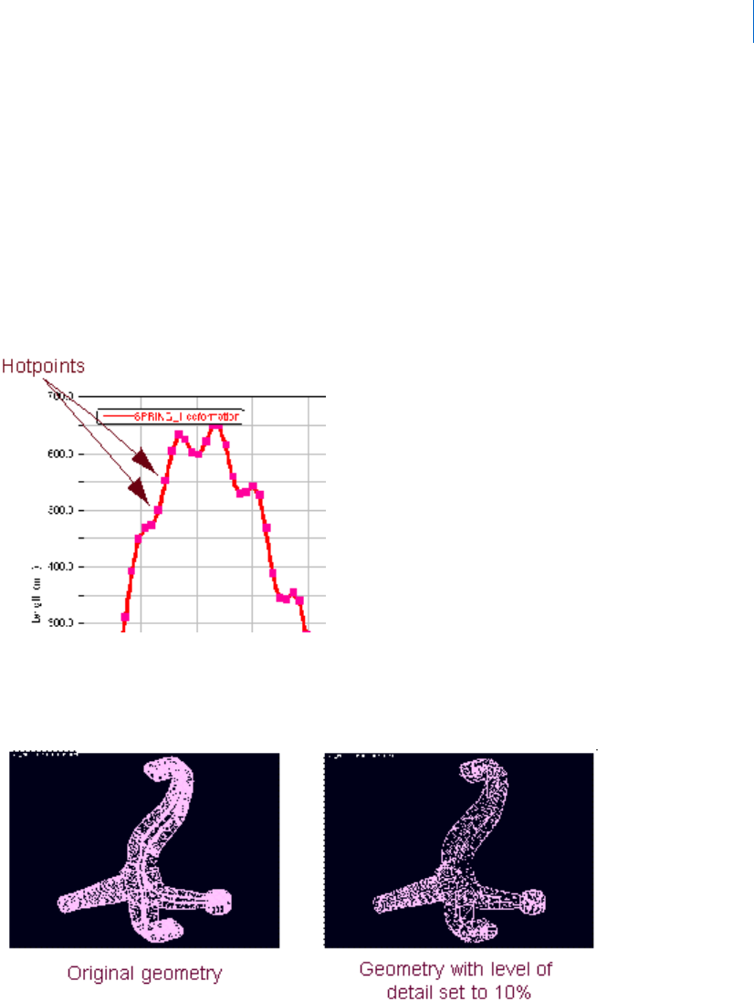
81
Appendix
Frequency-domain animations
Frequency-domain animations
Frequency-domain animations let you view your model oscillating at one of its natural frequencies. It cycles
through the model deformation starting from the operating point of the requested natural frequency of the
eigensolution. You can also see the effect of the damping on the model and display a table of eigenvalues.
Learn more About Frequency-Domain Animations.
Hotpoints
Small squares that appear on plot curves when selected. They enable you to change the data of the curve
manually.
Level of Detail Example
The following figure shows the impact of reducing a geometry’s level of detail to 10%.

Adams PostProcessor
Modes
82
Modes
Adams PostProcessor has four modes: animation, plotting, reports, and 3D plotting (only available with
Adams Vibration data). It switches its modes automatically depending on the contents of the active viewport.
For example, the tools in the Main toolbar change if you load an animation or a plot into a viewport. See
Viewports.
Notebooks
Notebooks are binary files that store all the simulation results, Animations, and plots that you are working
on in Adams PostProcessor in Stand-alone mode. To get results of simulations into your notebook, you
import the results.
Objects
Characteristics of objects in your model, such as the position of the center of mass of a part for the x
component. They correspond directly to object measures. To view objects, you must run Adams
PostProcessor with Adams View or import a Adams View command file.
Page
Pages display animations and plots. A page can have up to six Viewports.
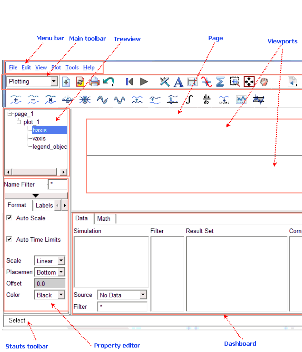
83
Appendix
Page
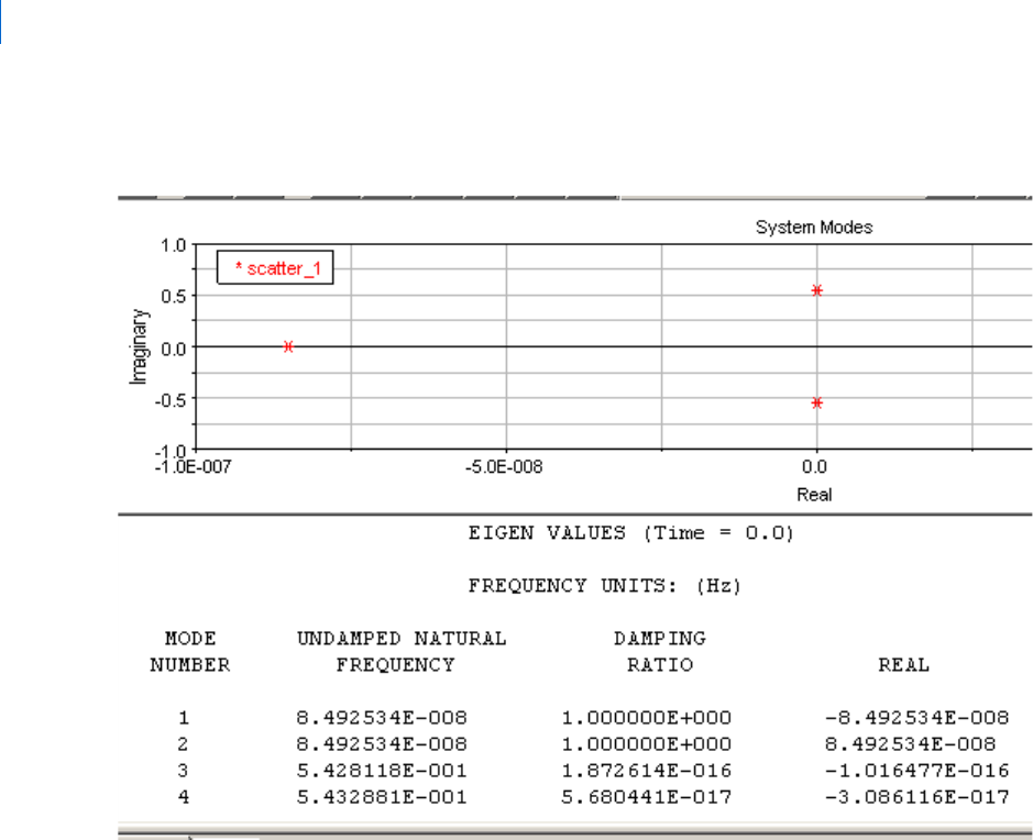
Adams PostProcessor
Picture of Plotting System Modes
84
Picture of Plotting System Modes
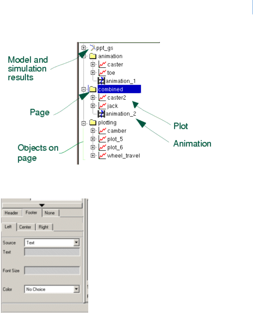
85
Appendix
Picture of Treeview
Picture of Treeview
Picture of property editor
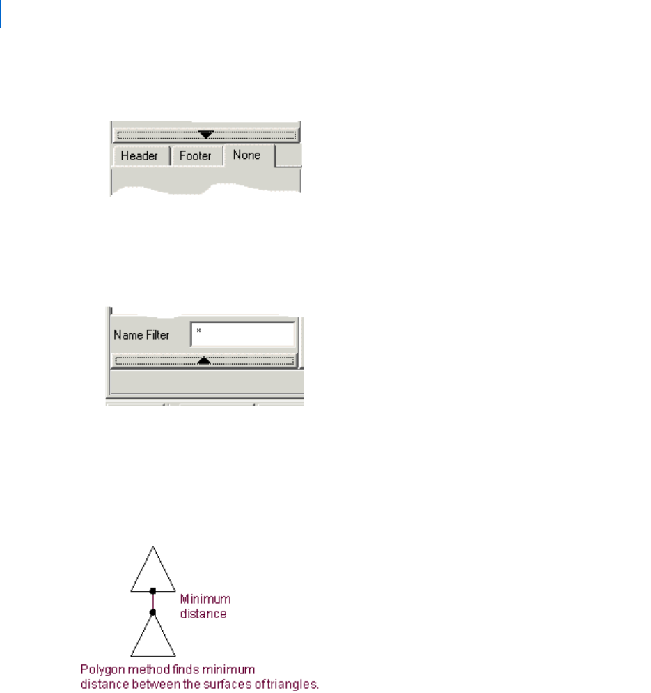
Adams PostProcessor
Picture of Property Editor Down Arrow
86
Picture of Property Editor Down Arrow
Picture Property Editor Up Arrow
Polygon
In the Polygon method, Adams PostProcessor calculates the minimum distance between the surfaces of the
triangles that make up the geometry. This is the most accurate method but requires the most time and
calculations. See also Vertex.
Property Editor
The Property Editor lets you change the properties of selected objects. It appears in the lower left corner of
the Adams PostProcessor window. The options in the Property Editor change depending on the element
selected in the Treeview.
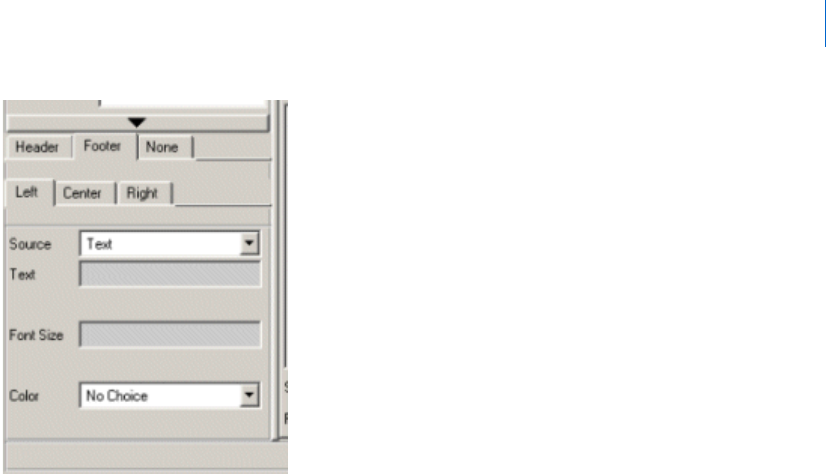
87
Appendix
Reports
Reports
Reports are data in simple HTML or ASCII format. For example, you can view the reports Adams
PostProcessor creates during a clearance study or create reports that help explain the plots and animations in
a presentation in Adams PostProcessor, much like the report displayed in the tutorial in
Getting Started Using
Adams PostProcessor
.
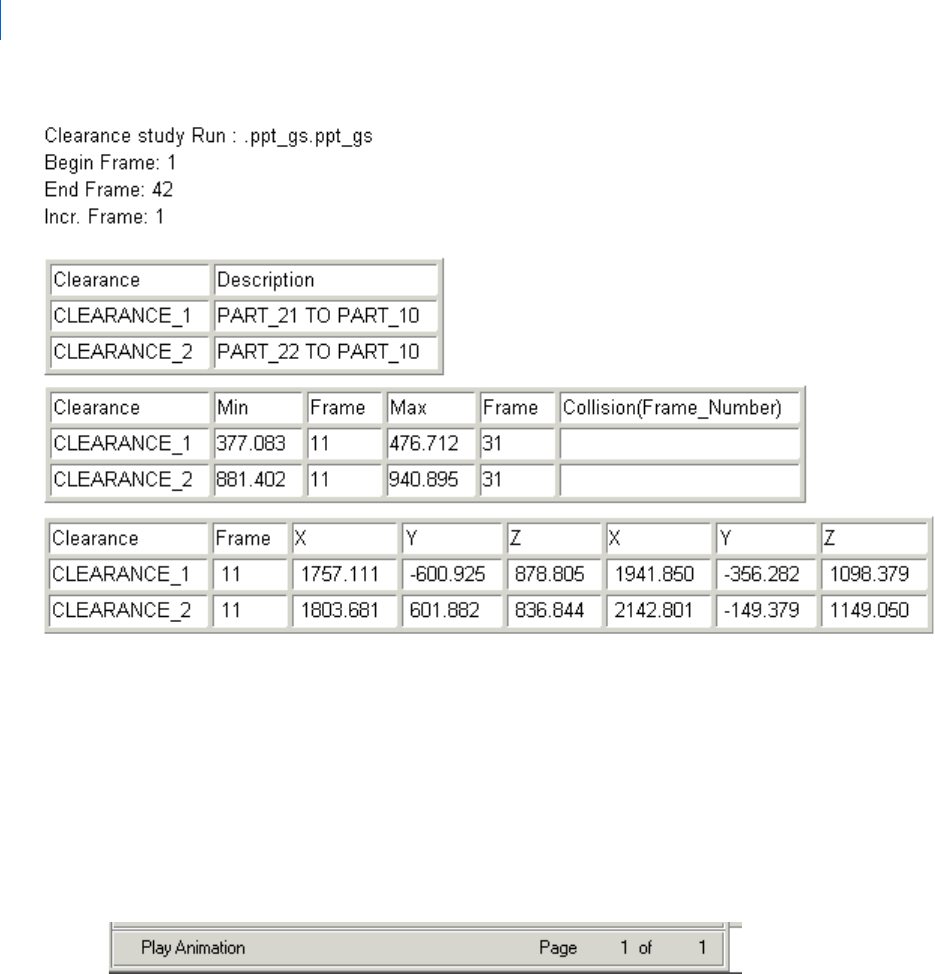
Adams PostProcessor
Stand-alone mode
88
Stand-alone mode
Stand-alone mode is when you start Adams PostProcessor separately from other Adams products. You can
also run it from within other Adams products, such as Adams View or Adams Car.
Status Bar
Displays information messages and prompts while you work. It appears at the bottom of the Adams
PostProcessor window.
Time-domain animations
A time-domain animation consists of one animation frame for every output step that you request in a time-
based Simulation in an Adams product, such as a Dynamic simulation in Adams View. For example, if you
performed a simulation from 0.0 to 10.0 seconds and asked for output every 0.1 seconds, Adams Solver
records data at 101 steps or frames. It creates a frame every tenth of a second for ten seconds plus one at time
0.0.
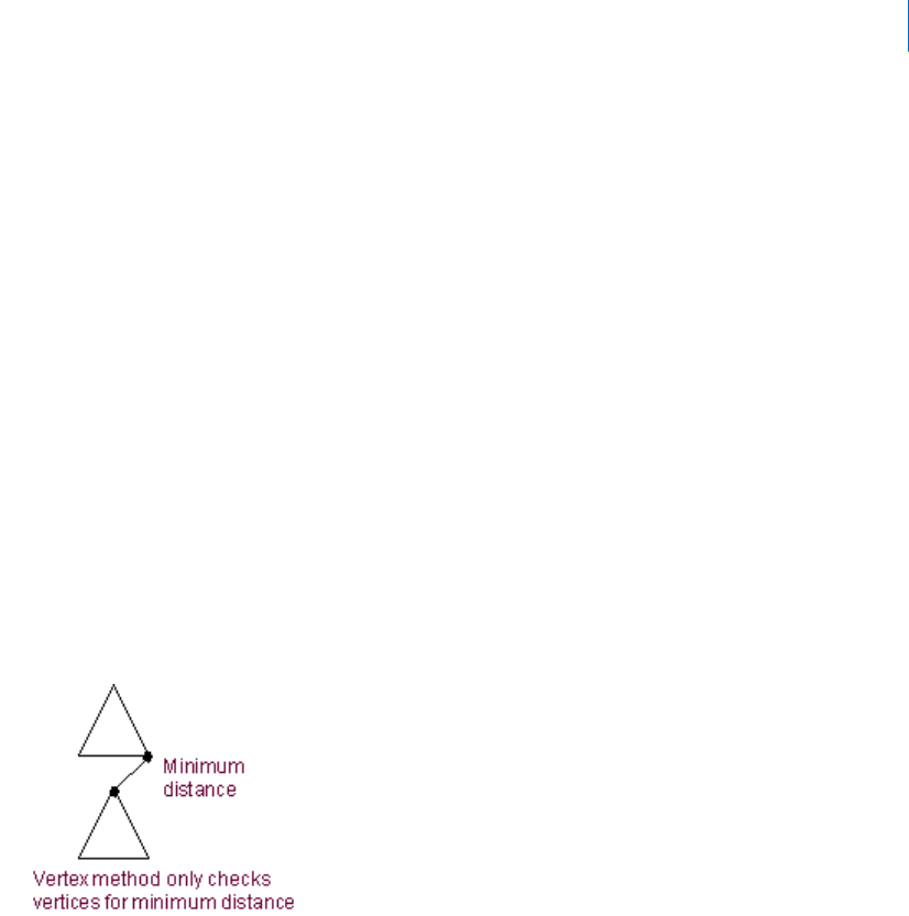
89
Appendix
Treeview
Treeview
The treeview is a hierarchical listing of objects in your current session. It appears along the left side of the
Adams PostProcessor window. A folder appears in front of each page in the tree to indicate that there are
objects stored on the page.
See About the Adams PostProcessor Window.
Learn more about Using the Treeview.
Vector plots
Vector plots display all three components of the vector at the same time. They consist of a force vector
attached to each node of a flexible body. You can select to animate modal forces (MFORCEs) acting on the
flexible body as vector plots to better visualize a result that is defined by its position on a body. Note that the
MNF must include nodal masses to use this feature.
See also Contour plots.
Vertex
In Vertex method, Adams PostProcessor calculates only the minimum distances between the vertices of the
triangles that make up the geometry. This method is less accurate than Polygon, but calculates faster.
Viewports
Rectangular areas of the window that display different views of plots, animations, or reports. You can place
up to six viewports on a page. Adams PostProcessor provides you with 12 viewport layouts from which you
can choose.

Adams PostProcessor
Viewports
90
