Introduction to Application Builder

COMSOL Multiphysics

Application Programming Guide

Contact Information

Visit the Contact COMSOL page at www.comsol.com/contact to submit general inquiries, contact

Technical Support, or search for an address and phone number. You can also visit the Worldwide

Sales Offices page at www.comsol.com/contact/offices for address and contact information.

If you need to contact Support, an online request form is located at the COMSOL Access page at

www.comsol.com/support/case. Other useful links include:

• Support Center: www.comsol.com/support

• Product Download: www.comsol.com/product-download

• Product Updates: www.comsol.com/support/updates

•COMSOL Blog: www.comsol.com/blogs

• Discussion Forum: www.comsol.com/community

•Events: www.comsol.com/events

• COMSOL Video Gallery: www.comsol.com/video

• Support Knowledge Base: www.comsol.com/support/knowledgebase

Part number: CM020012

Application Programming Guide

Protected by patents listed on www.comsol.com/patents, and U.S. Patents 7,519,518; 7,596,474; 7,623,991; 8,457,932;

8,954,302; 9,098,106; 9,146,652; 9,323,503; 9,372,673; 9,454,625; and 10,019,544. Patents pending.

This Documentation and the Programs described herein are furnished under the COMSOL Software License

Agreement (www.comsol.com/comsol-license-agreement) and may be used or copied only under the terms of the

license agreement.

COMSOL, the COMSOL logo, COMSOL Multiphysics, COMSOL Desktop, COMSOL Compiler, COMSOL Server,

and LiveLink are either registered trademarks or trademarks of COMSOL AB. All other trademarks are the property

of their respective owners, and COMSOL AB and its subsidiaries and products are not affiliated with, endorsed by,

sponsored by, or supported by those trademark owners. For a list of such trademark owners, see www.comsol.com/

trademarks.

Version: COMSOL 5.5

| 3

Contents

Introduction . . . . . . . . . . . . . . . . . . . . . . . . . . . . . . . . . . . . . . . . . . . 7

Syntax Primer . . . . . . . . . . . . . . . . . . . . . . . . . . . . . . . . . . . . . . . . . . 8

Data Types. . . . . . . . . . . . . . . . . . . . . . . . . . . . . . . . . . . . . . . . . . 8

Declarations. . . . . . . . . . . . . . . . . . . . . . . . . . . . . . . . . . . . . . . . 14

Built-in Elementary Math Functions. . . . . . . . . . . . . . . . . . . . . 15

Control Flow Statements. . . . . . . . . . . . . . . . . . . . . . . . . . . . . 15

Important Programming Tools . . . . . . . . . . . . . . . . . . . . . . . . . . . 18

Ctrl+Space for Code Completion . . . . . . . . . . . . . . . . . . . . . 18

Recording Code . . . . . . . . . . . . . . . . . . . . . . . . . . . . . . . . . . . . 20

Methods Called from the Model Builder . . . . . . . . . . . . . . . . 23

Global Methods, Form Methods, and Local Methods . . . . . 23

Method Names . . . . . . . . . . . . . . . . . . . . . . . . . . . . . . . . . . . . . 24

Introduction to the Model Object. . . . . . . . . . . . . . . . . . . . . . . . 25

Model Object Tags . . . . . . . . . . . . . . . . . . . . . . . . . . . . . . . . . . 25

Creating a Model Object . . . . . . . . . . . . . . . . . . . . . . . . . . . . . 28

Creating Model Components and Model Object Nodes . . 28

Get and Set Methods for Accessing Properties . . . . . . . . . . 29

Parameters and Variables. . . . . . . . . . . . . . . . . . . . . . . . . . . . . 34

Unary and Binary Operators in the Model Object . . . . . . . . 36

Geometry. . . . . . . . . . . . . . . . . . . . . . . . . . . . . . . . . . . . . . . . . . 37

Mesh . . . . . . . . . . . . . . . . . . . . . . . . . . . . . . . . . . . . . . . . . . . . . . 39

Physics . . . . . . . . . . . . . . . . . . . . . . . . . . . . . . . . . . . . . . . . . . . . 40

Material. . . . . . . . . . . . . . . . . . . . . . . . . . . . . . . . . . . . . . . . . . . . 42

Study. . . . . . . . . . . . . . . . . . . . . . . . . . . . . . . . . . . . . . . . . . . . . . 44

Results . . . . . . . . . . . . . . . . . . . . . . . . . . . . . . . . . . . . . . . . . . . . 48

4 |

Multiphysics . . . . . . . . . . . . . . . . . . . . . . . . . . . . . . . . . . . . . . . . 50

Working with Model Objects . . . . . . . . . . . . . . . . . . . . . . . . . 51

The Model Object Class Structure. . . . . . . . . . . . . . . . . . . . . 53

The Application Object . . . . . . . . . . . . . . . . . . . . . . . . . . . . . . . . 55

Shortcuts . . . . . . . . . . . . . . . . . . . . . . . . . . . . . . . . . . . . . . . . . . 55

Accessing the Application Object. . . . . . . . . . . . . . . . . . . . . . 57

The Name of User Interface Components . . . . . . . . . . . . . . 57

Important Classes . . . . . . . . . . . . . . . . . . . . . . . . . . . . . . . . . . . 57

Get and Set Methods for the Color of a Form Object . . . . 58

General Properties . . . . . . . . . . . . . . . . . . . . . . . . . . . . . . . . . . 59

The Main Application Methods. . . . . . . . . . . . . . . . . . . . . . . . 60

Main Window . . . . . . . . . . . . . . . . . . . . . . . . . . . . . . . . . . . . . . 61

Form. . . . . . . . . . . . . . . . . . . . . . . . . . . . . . . . . . . . . . . . . . . . . . 62

Form Object . . . . . . . . . . . . . . . . . . . . . . . . . . . . . . . . . . . . . . . 63

Item . . . . . . . . . . . . . . . . . . . . . . . . . . . . . . . . . . . . . . . . . . . . . . 83

Data Source. . . . . . . . . . . . . . . . . . . . . . . . . . . . . . . . . . . . . . . . 84

Method Class . . . . . . . . . . . . . . . . . . . . . . . . . . . . . . . . . . . . . . 89

Form, Form Object, and Item List Methods . . . . . . . . . . . . . 89

The Built-in Method Library for the Application Builder. . . . . . 91

Model Utility Methods . . . . . . . . . . . . . . . . . . . . . . . . . . . . . . . 91

License Methods . . . . . . . . . . . . . . . . . . . . . . . . . . . . . . . . . . . . 93

File Methods . . . . . . . . . . . . . . . . . . . . . . . . . . . . . . . . . . . . . . . 96

Operating System Methods. . . . . . . . . . . . . . . . . . . . . . . . . . 103

Email Methods. . . . . . . . . . . . . . . . . . . . . . . . . . . . . . . . . . . . . 107

Email Class Methods. . . . . . . . . . . . . . . . . . . . . . . . . . . . . . . . 107

GUI-Related Methods . . . . . . . . . . . . . . . . . . . . . . . . . . . . . . 111

GUI Command Methods. . . . . . . . . . . . . . . . . . . . . . . . . . . . 122

Debug Methods . . . . . . . . . . . . . . . . . . . . . . . . . . . . . . . . . . . 123

| 5

Methods for External C Libraries . . . . . . . . . . . . . . . . . . . . .123

Progress Methods . . . . . . . . . . . . . . . . . . . . . . . . . . . . . . . . . .125

Date and Time Methods . . . . . . . . . . . . . . . . . . . . . . . . . . . .131

Conversion Methods . . . . . . . . . . . . . . . . . . . . . . . . . . . . . . .134

Array Methods . . . . . . . . . . . . . . . . . . . . . . . . . . . . . . . . . . . .136

String Methods . . . . . . . . . . . . . . . . . . . . . . . . . . . . . . . . . . . .144

Collection Methods . . . . . . . . . . . . . . . . . . . . . . . . . . . . . . . .145

Model Builder Methods for Use in Add-ins. . . . . . . . . . . . .148

Programming Examples. . . . . . . . . . . . . . . . . . . . . . . . . . . . . . . . 150

Running the Examples . . . . . . . . . . . . . . . . . . . . . . . . . . . . . .150

Visualization Without Solution Data: Grid Data Sets. . . . .150

Visualization of Points, Curves, and Surfaces . . . . . . . . . . . .152

Reading and Writing Data to File . . . . . . . . . . . . . . . . . . . . .162

Converting Interpolation Curve Data. . . . . . . . . . . . . . . . . .186

Plotting Points on a Parametric Surface . . . . . . . . . . . . . . . .188

Using Selections for Editing Geometry Objects . . . . . . . . .189

Recursion and Recursively Defined Geometry Objects. . .194

Mesh Information and Statistics. . . . . . . . . . . . . . . . . . . . . . .198

Accessing Higher-Order Finite Element Nodes . . . . . . . . .199

Accessing System Matrices and Vectors. . . . . . . . . . . . . . . .201

Using Built-In Methods from an External Java Library. . . . .205

Measuring the Java Heap Space Memory. . . . . . . . . . . . . . .206

Time-Limited and Hardware-Locked Applications . . . . . . .206

6 |

| 7

Introduction

This book is a guide to writing code for COMSOL

models and applications

using the Method editor. The Method editor is an important part of the

Application Builder and is available in the COMSOL Desktop

environment in

the Windows

version of COMSOL Multiphysics. For an introduction to using

the Application Builder and its Form editor and Method editor, see the book

Introduction to Application Builder.

Writing a method is needed when an action is not already available in the standard

run commands associated with functionality in the model tree nodes of the Model

Builder. A method may, for example, contain loops, process inputs and outputs,

and send messages and alerts to the user of the application.

In the Model Builder, the model tree is a graphical representation of the data

structure that represents a model. This data structure is called the model object

and stores the state of the underlying COMSOL Multiphysics model that is

embedded in an application.

The contents of the application tree in the Application Builder is accessed through

the application object, which is an important part of the model object. You can

write code using the Method editor to directly access and change the user interface

of a running application, for example, to update button text, icons, colors, and

fonts.

In the COMSOL Multiphysics environment, you use the Java

programming

language to write methods, which means that you can utilize the extensive

collection of Java

libraries. In addition to the Java

libraries, the Application

Builder includes a built-in library for building applications and modifying the

model object. A number of tools and resources are available to help you

automatically create code for methods. For more information on autogeneration

of code, see the book Introduction to Application Builder.

This book assumes no prior knowledge of the Java

programming language.

However, some familiarity with a programming language is helpful.

8 |

Syntax Primer

If you are not familiar with the Java

programming language, read this section to

quickly get up to speed with its syntax. When creating applications, it is useful to

know the basics of Java such as how to use the

if, for, and while control

statements. The more advanced aspects of Java will not be covered in this book.

For more detail, see any dedicated book on Java

programming or one of the many

online resources. You can also learn a lot by reviewing the methods in the example

applications available in the Application Libraries.

Data Types

RIMITIVE DATA TYPES

Java contains eight primitive data types, listed in the table below.

Other data types such as strings are classes, which are also referred to as composite

data types.

In methods, you can use any

of the primitive or composite data types available in

Java and the Java libraries. Many of the Application Builder built-in methods make

use of primitive or composite data types. For example, the

timeStamp() method

provides a

long integer as its output.

ASSIGNMENTS AND LITERALS

A few examples of using literals in assignments are:

DATA TYPE DESCRIPTION NUMBER OF BYTES EXAMPLE

byte

Integer between -127 and 128 1 byte b=33;

char

Unicode character; integer between

0 and 65535 (0 and 2

-1)

2 char c=’a’;

char c=97;

short

Integer between -32768 and 32767

(-2

-1 and 2

-1)

2 short s=-1025;

int

Integer between -2

and 2

-1 4 int i=15;

long

Integer between -2

and 2

-1 8 long l=15;

float

32-bit floating point number 4 float f =4.67f;

double

64-bit floating point number 8 double d=4.67;

boolean

Boolean with values false or true N/A boolean b=true;

| 9

int i=5; // initialize i and assign the value 5

double d=5.0; // initialize d and assign the value 5.0

boolean b=true; // initialize b and assign the value true

The constants 5, 5.0, and true are literals. Java distinguishes between the literals

5 and 5.0, where 5 is an integer and 5.0 is a double (or float).

UNARY AND BINARY OPERATORS IN METHODS (JAVA SYNTAX)

You can perform calculations and operations using primitive data types just like

with many other programming languages. The table below describes some of the

most common unary and binary operators used in Java code.

TYPE CONVERSIONS AND TYPE CASTING

When programming in Java, conversion between data types is automatic in many

cases. For example, the following lines convert from an integer to a double:

int i; // initialize i

double d; //initialize d

i=41;

d=i; // the integer i is assigned to the double d and d is 41.0

However, the opposite will not work automatically (you will get a compilation

error). Instead you can use explicit type casting as follows:

PRECEDENCE LEVEL SYMBOL DESCRIPTION

1 ++ -- unary: postfix addition and subtraction

2 ++ -- + - ! unary: addition, subtraction, positive sign,

negative sign, logical not

3 * / % binary: multiplication, division, modulus

4 + - binary: addition, subtraction

5 ! Logical NOT

6 < <= > >= comparisons: less than, less than or equal,

greater than, greater than or equal

7 == != comparisons: equal, not equal

8 && binary: logical AND

9 || binary: logical OR

10 ?: conditional ternary

11 = += -= *= /=

%= >>= <<= &=

^= |=

assignments

12 , element separator in lists

10 |

int i; // initialize i

double d; //initialize d

d=41.0;

i=(int) d; // the double d is assigned to the integer i and i is 41

You can convert between integers and doubles within arithmetic statements in

various ways, however you will need to keep track of when the automatic type

conversions are made. For example:

int i; // initialize i

double d; //initialize d

i=41;

d=14/i; // d is 0

In the last line, 14 is seen as an integer literal and the automatic conversion to a

double is happening after the integer division

14/41, which results in 0.

Compare with:

int i; // initialize i

double d; //initialize d

i=41;

d=14.0/i; // d is 0.3414...

In the last line, 14.0 is seen as a double literal and the automatic conversion to a

double is happening before the division and is equivalent to

14.0/41.0.

You can take charge over the type conversions with explicit casting by using the

syntax

(int) or (double):

int i; // initialize i

double d,e; //initialize d and e

i=41;

d=((int) 14.0)/i; // d is 0

e=14/((double) i); // e is 0.3414...

STRINGS AND JAVA OBJECTS

The String data type is a Java object. This is an example of how to declare a string

variable:

String a="string A";

When declaring a string variable, the first letter of the data type is capitalized. This

is a convention for composite data types (or object-oriented classes).

After you have declared a string variable, a number of methods are automatically

made available that can operate on the string in various ways. Two such methods

are

concat and equals as described below, but there are many more methods

available in the

String class. See the online Java documentation for more

information.

Concatenating Strings

To concatenate strings, you can use the method concat as follows:

| 11

String a="string A";

String b=" and string B";

a.concat(b);

The resulting string a is "string A and string B". From an object-oriented

perspective, the variable

a is an instance of an object of the class String. The

method

concat is defined in the String class and available using the a.concat()

syntax.

Alternatively, you can use the

+ operator as follows:

a=a+b;

which is equivalent to:

a="string A" + " and string B";

and equivalent to:

a="string A" + " " + "and string B";

where the middle string is a string with a single whitespace character.

Comparing Strings

Comparing string values in Java is done with the equals method and not with the

== operator. This is due to the fact that the == operator compares whether the

strings are the same when viewed as class objects and does not consider their

values. The code below demonstrates string comparisons:

boolean streq=false;

String a="string A";

String b="string B";

streq=a.equals(b);

// In this case streq==false

streq=(a==b);

// In this case streq==false

b="string A";

streq=a.equals(b);

// In this case streq==true

Special Characters

If you would like to store, for example, a double quotation mark or a new line

character in a string you need to use special character syntax preceded by a

backslash (\). The table below summarizes some of the most important special

characters.

SPECIAL CHARACTER DESCRIPTION

Single quotation mark

Double quotation mark

12 |

Note that in Windows the new line character is the composite \r\n whereas in

Linux and macOS

\n is used.

The example below shows how to create a string in Windows that you later on

intend to write to file and that consists of several lines.

String contents = "# Created by me\r\n"

+"# Version 1.0 of this file format \r\n"

+"# Body follows\r\n"

+"0 1 \r\n"

+"2 3\r\n"

+"4 5\r\n";

The string is here broken up into several lines in the code for readability. However,

the above is equivalent to the following:

String contents = "# Created by me\r\n# Version 1.0 of this file format \r\n#

Body follows\r\n0 1 \r\n2 3\r\n4 5\r\n

which is clearly less readable.

ARRAYS

In the application tree, the Declarations node directly supports 1D and 2D arrays

of type string (

String), integer (int), Boolean (boolean), or double (double). A

1D array may be referred to as a vector and a 2D array referred to as a matrix,

provided that the array is rectangular. A non-rectangular array is called jagged or

ragged. In methods, you can define higher-dimensional arrays as well as arrays of

data types other than string, integer, Boolean, or double.

1D Arrays

If you choose not to use the Declarations node to declare an array, then you can

use the following syntax in a method:

double dv[] = new double[12];

This declares a double array of length 12.

The previous line is equivalent to the following two lines:

double dv[];

dv = new double[12];

Backslash

Tab

Backspace

Carriage return

Formfeed

Newline

SPECIAL CHARACTER DESCRIPTION

| 13

When a double vector has been declared in this way, the value of each element in

the array will be zero.

To access elements in an array you use the following syntax:

double e;

e=dv[3]; // e is 0.0

Arrays are indexed starting from 0. This means that dv[0] is the first element of

the array in the examples above, and

dv[11] is the last element.

You can simultaneously declare and initialize the values of an array by using curly

braces:

double dv[] = {4.1, 3.2, 2.93, 1.3, 1.52};

In a similar way you can create an array of strings as follows:

String sv[] = {"Alice", "Bob", "Charles", "David", "Emma"};

2D Arrays

2D rectangular arrays can be declared as follows:

double dm[][] = new double[2][3];

This corresponds to a matrix of doubles with 2 rows and 3 columns. The row

index comes first.

You can simultaneously declare and initialize a 2D array as follows:

double dm[][] = {{1.32, 2.11, 3.43},{4.14, 5.16, 6.12}};

where the value of, for example, dm[1][0] is 4.14. This array is a matrix since it is

rectangular (it has same number of columns for each row). You can declare a

ragged array as follows:

double dm[][] = {{1.32, 2.11}, {4.14, 5.16, 6.12, 3.43}};

where the value of, for example, dm[1][3] is 3.43.

Copying Arrays

For copying arrays, the following code:

for(int i1=0;i1<=11;i1++) {

for(int i2=0;i2<=2;i2++) {

input_array[i1][i2]=init_input_array[i1][i2];

}

is not equivalent to the line:

input_array=init_input_array;

since the last line will only copy by reference.

Instead, you can use the

copy method as follows:

input_table = copy(init_input_table);

which allocates a new array and then copies the values.

14 |

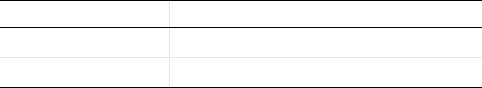
Declarations

Variables defined in the Declarations node in the application tree are directly

available as global variables in a method and need no further declarations.

Variables declared in methods will have local scope unless you specify otherwise.

The

Declarations node directly supports integers (int), doubles (double), and

Booleans (

boolean). In addition, strings are supported (see “Strings and Java

Objects” on page 10). In the

Declarations node, variables can be scalars, 1D arrays,

and 2D arrays.

To simplify referencing form objects as well as menu, ribbon, and toolbar items by

name, you can create shortcuts with a custom name. These names are available in

the

Declarations node under Shortcuts. They are directly available in methods along

with the other global variables defined under

Declarations. For more information

on shortcuts, see “Shortcuts” on page 55.

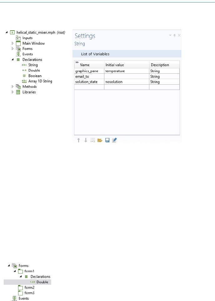
FORM DECLARATIONS

Variables can also be defined as Form Declarations under each respective form node

in the application tree.

| 15

Form declarations can be of the types Scalar, Array 1D, Array 2D and Choice List.

Global declarations are exposed to all components of the application whereas form

declarations are only exposed to the form that they are defined in and the form

objects within that form. Form declarations are used to limit the scope of variables

and thereby logically separate the different parts of an application.

Built-in Elementary Math Functions

Elementary math function for use in methods are available in the Java math library.

Some examples:

double a = Math.PI; // the mathematical constant pi

double b = Math.sin(3*a); // trigonometric sine function

double c = Math.cos(4*a); // trigonometric cosine function

double d = Math.random(); // random number uniformly distributed in [0,1)

double e = Math.exp(2*a); // exponential function

double f = Math.log(1+e); // natural base e logarithm

double g = Math.pow(10,3) // power function

double h = Math.log10(2.5); // base 10 logarithm

double k = Math.sqrt(81.0); // square root

There are several more math functions available in the Java math library. For

additional information, see any Java book or online resource.

Control Flow Statements

Java supports the usual control flow statements if-else, for, and while. The

following examples illustrate some of the most common uses of control flow

statements.

THE IF-ELSE STATEMENT

This is an example of a general if-else statement:

if(a<b) {

alert("Value too small.");

} else {

alert("Value is just right.");

}

Between curly braces {} you can include multiple lines of code, each terminated

with a semicolon. If you only need one line of code, such as in the example above,

this shortened syntax is available:

if(a<b)

alert("Value too small.");

16 |

else

alert("Value is just right.");

THE FOR STATEMENT

Java supports several different types of for statements. This example uses the

perhaps most conventional syntax:

// Iterate i from 1 to N:

int N=10;

for (int i = 1; i <= N; i++) {

// Do something

}

An alternative syntax is shown in the example on page 64 where the loop is over

all form objects in a list of form objects:

for (FormObject formObject : app.form("form1").formObject()) {

if ("Button".equals(formObject.getType())) {

formObject.set("enabled", false);

}

where the local iteration variable looped over is formObject of the type, or class,

FormObject. The collection of objects, in this case

app.form("form1").formObject(), can be an array or other types of lists of

objects. Using this syntax, the iteration variable loops over all entries in the

collection, from start to finish. Another example can be found on page 90.

THE WHILE STATEMENT

This example shows a while statement.

double t=0,h=0.1,tend=10;

while(t<tend) {

//do something with t

t=t+h;

}

For a more advanced example of a while statement, see “Creating and Removing

Model Tree Nodes” on page 41.

Note that Java also supports

do-while statements.

THE WITH STATEMENT

When writing methods in the Method editor, in addition to the standard Java

control flow statement, there is also a

with statement that is used to make

Application Builder code more compact and easier to read. A simple example is

shown below:

// Set the global parameter L to a fixed value

with(model.param());

| 17

set("L", "10[cm]");

endwith();

The code above is equivalent to:

model.param().set("L", "10[cm]");

In this case using the with statement has limited value since just one parameter is

assigned but for multiple assignments readability increases. See “Parameters and

Variables” on page 34 for an example with multiple assignments.

Note that the

with statement is only available when writing code in the Method

editor. It is not available when using the COMSOL API for use with Java

. You

can turn off the use of

with statements in the section for Methods in Preferences.

The method

descr returns the variable description for the last parameter or

variable in a

with statement:

with(model.param());

set("L", "10[cm]");

String ds = descr("L");

endwith();

Assuming that the parameter description of the parameter L is Length. The string

ds will have the value Length.

EXCEPTION HANDLING

An exception is an error that occurs at run time. The Java

programming language

has a sophisticated machinery for handling exceptions and each exception

generates an object of an exception class. The most common way to handle

exceptions is by using

try and catch, as in the example below.

double d[][] = new double[2][15];

try {

d = readMatrixFromFile(

"common:///my_file.txt");

} catch (Exception e) {

error(

"Cannot find the file my_file.txt.");

}

where an error dialog box is shown in case the file my_file.txt is not found in

the application file folder

common. See the Java

documentation for more

information about using

try and catch.

18 |

Important Programming Tools

The Application Builder includes several tools for automatically generating code.

These tools include code completion,

Record Method, Record Code, Convert to New

Method

, Editor Tools, Language Elements, and Copy as Code to Clipboard, and are

described in the book Introduction to Application Builder. These utilities allow

you to quickly get up and running with programming tasks even if you are not

familiar with the syntax.

The following sections describes two of the most important tools: code

completion using Ctrl+Space and

Record Code. Using these tools will make you

more productive, for example, by allowing you to copy-paste or auto-generate

blocks of code.

Ctrl+Space for Code Completion

While typing code in the Method editor, the Application Builder can provide

suggestions for code completions. The list of possible completions are shown in a

separate completion list that opens while typing. In some situations, detailed

information appears in a separate window when an entry is selected in the list.

Code completion can always be requested with the keyboard shortcut Ctrl+Space.

Alternatively Ctrl+/ can be used to request code completion, which is useful if

Ctrl+Space is in use by the Windows operating system such as for certain

languages. When accessing parts of the model object, you will get a list of possible

completions, as shown in the figure below:

Select a completion by using the arrow keys to choose an entry in the list and

double-click, or press the Tab or Enter key, to confirm the selection.

If the list is long, you can filter by typing the first few characters of the completion

you are looking for.

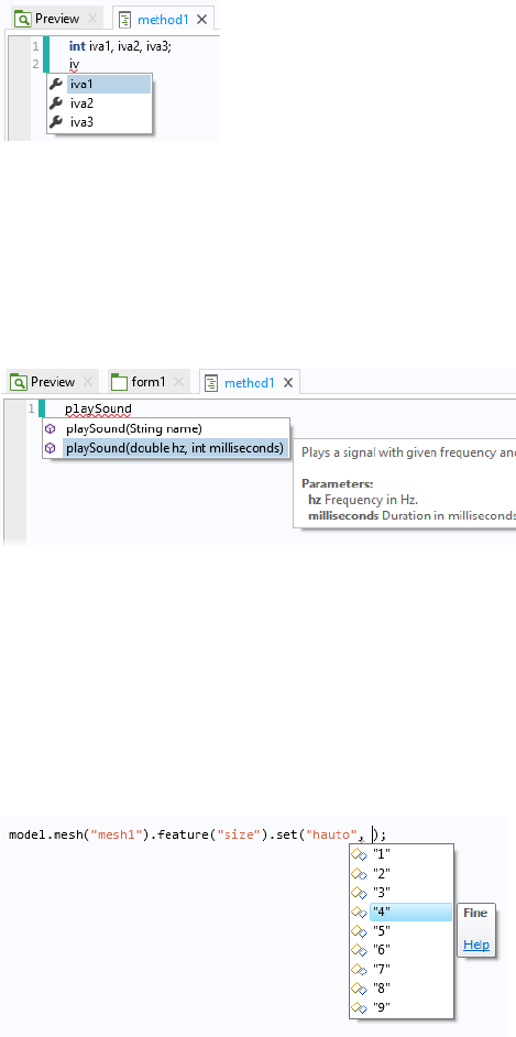
| 19

For example, if you enter the first few characters of a variable or method name,

and press Ctrl+Space, the possible completions are shown:

In the example above, only variables that match the string

iv are shown. This

example shows that variables local to the method also appear in the completion

suggestions.

You can also use Ctrl+Space to learn about the syntax for the built-in methods that

are not directly related to the model object. Type the name of the command and

use Ctrl+Space to open a window with information on the various calling

signatures available.

Additional information is also available in the form of tool tips that are displayed

when hovering over the different parts of the code.

The Method editor also supports code completion for properties, including listing

the properties that are available for a given model object feature node, and

providing a list of allowed values that are available for a given property.

The figure below shows an example of code completion for the mesh element size

property, where a list of the allowed values for the predefined element sizes is

presented.

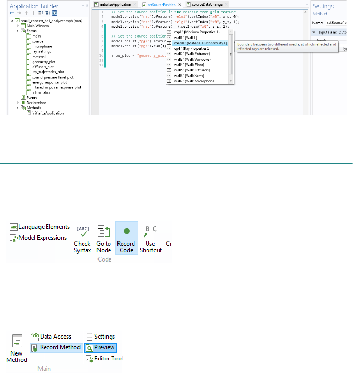
20 |

COMSOL Multiphysics and its add-on modules contain thousands of physics

features that you can learn about by using, for example,

Record Code, Save

as>Model File for Java

, and code completion. The figure below shows code

completion for a particular feature in the Ray Optics Module.

Recording Code

Click the Record Code button in the Code section of the Method editor ribbon to

record a sequence of operations that you perform using the model tree, as shown

in the figure below.

Certain operations in the application tree can also be recorded, for example, code

that changes the color of a text label in a running application may be generated.

To record a new method, click the

Record Method button in the Main section of

the Method editor ribbon.

| 21

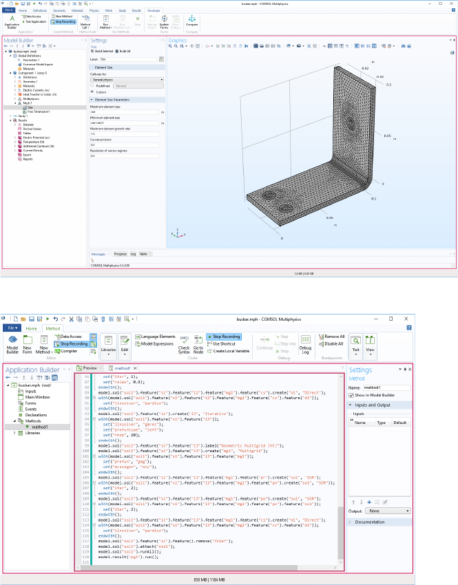
While recording code, the COMSOL Desktop windows are surrounded by a red

frame:

22 |

To stop recording code, click one of the Stop Recording buttons in the ribbon of

either the Model Builder or the Application Builder.

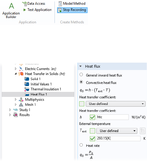
By using

Data Access, you can set the values of the Heat transfer coefficient and the

External temperature properties of the busbar tutorial model used in the books

Introduction to COMSOL Multiphysics and Introduction to Application

Builder.

To generate similar code using

Record Code (Data Access is not used when

recording code), follow these steps:

• Create a simple application based on the busbar model (MPH file).

• In the Model Builder window, in the Developer tab, click Record Method, or

with the Method editor open, click

Record Code.

• Change the value of the Heat transfer coefficient to 5.

• Change the value of the External temperature to 300[K].

• Click Stop Recording.

• If it is not already open, open the method with the recorded code.

The resulting code is listed below:

with(model.physics("ht").feature("hf1"));

set("h", "5");

set("Text", "300[K]");

endwith();

| 23

In this case, the autogenerated code contains a with() statement in order to make

the code more compact. For more information on the use of

with(), see “The

With Statement” on page 16.

To generate code corresponding to changes to the application object, use

Record

Code

or Record Method, then go to the Form editor and, for example, change the

appearance of a form object. The following code corresponds to changing the

color of a text label from the default

Inherit to Blue:

with(app.form("form1").formObject("textlabel1"));

set("foreground", "blue");

endwith();

Built-in methods that changes the application object are only available when

running applications and not when running methods from the Model Builder.

Use the tools for recording code to quickly learn how to interact with the model

object or the application object. The autogenerated code shows you the names of

properties, parameters, and variables. Use strings and string-number conversions

to assign new parameter values in model properties. By using

Data Access while

recording, you can, for example, extract a parameter value using

get, process its

value in a method, and save it back into the model object using

set. For more

information on

Data Access, see the Introduction to Application Builder.

Methods Called from the Model Builder

Methods called from the Model Builder directly modify the model object

represented by the Model Builder in the current session. Using methods in this

way can be used to automate modeling tasks that consist of several manual steps.

For example, in a model with multiple studies, you can record code for the process

of first computing Study 1; then computing Study 2, which may be based on the

solution from Study 1; and so on.

To customize the workflow in the Model Builder you can create an add-in based

on methods by using a

Method Call or a Settings Form. For an introductory example

of using methods from the Model Builder and for information on how to create

add-ins, see the Introduction to Application Builder.

Global Methods, Form Methods, and Local Methods

There are global methods, form methods, and local methods. Global methods are

displayed in the application tree and are accessible from all methods and form

objects. Form methods are displayed in the application tree as child nodes to the

24 |

form it belongs to. A local method is associated with a form object or event and

can be opened from the corresponding

Settings window.

Global methods are exposed to all components of the application whereas form

methods are only exposed to the form that they are defined in and the form objects

within that form. You can use form methods to provide a logical separation of the

different parts of an application.

Method Names

A method name has to be a text string without spaces. The string can contain

letters, numbers, and underscores. Java® programming language keywords

cannot be used. The name must not begin by a number (this is also true for the

name of a form object, variable, and method.)

A global method cannot have the same name as a form method and vice versa. In

addition, the following names are reserved:

• onDataChange

• onPickingChanged

• focusGained

• focusLost

• onLoad

• onClose

• onStartup

• onShutdown

• onClick

• onEvent

| 25

Introduction to the Model Object

The model object is the data structure that stores the state of the COMSOL

Multiphysics model. The model object contents are reflected in the COMSOL

Desktop user interface by the structure of the Model Builder and its model tree.

The model object is associated with a large number of methods for setting up and

running sequences of operations such as geometry sequences, mesh sequences,

and study steps. As an alternative to using the Model Builder, you can write

programs in the Method editor that directly access and change the contents of the

model object.

The model object methods are structured in a tree-like way, similar to the nodes

in the model tree. The top-level methods just return references that support

further methods. At a certain level the methods perform actions, such as adding

data to the model object, performing computations, or returning data.

For a complete list of methods used to edit the model object, see the

Programming Reference Manual. For an introduction to using the Model

Builder, see the book Introduction to COMSOL Multiphysics.

The contents of the application tree in the Application Builder are accessed

through the application object, which is an important part of the model object.

You can write code using the Method editor to alter, for example, button text,

icons, colors, and fonts in the user interface of a running application.

This section gives an overview of the model object. The section “The Application

Object” on page 55 gives an overview of the application object.

Model Object Tags

In the model tree and when working with the model object from methods, tags

are used as handles to different parts of the model object. These tags can also be

26 |

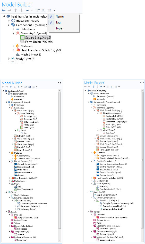
made visible in the Model Builder by first clicking the Model Builder toolbar

Model Tree Node Text and then choosing Tag, as shown in the figure below.

The figures below show an example of a model tree without tags shown in the left

figure and with tags shown in the right figure.

| 27

In code, the tags are referenced using double quotes. For example, in the

following line

model.geom("geom1").create("r1", "Rectangle");

geom1 is a tag for a geometry object and r1 is a tag for a rectangle object. The

following sections contain multiple examples of using tags to create and edit parts

of a model object.

The option

Name, available in the Model Tree Node Text menu in the Model Builder

toolbar, represents the name used for scoping. The scope names are used to access

the different parts of the model object. This is important, for example, when

working with global variables for defining the constraints and objective functions

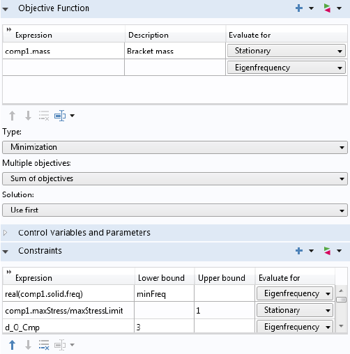
for an optimization study. In the figure below, the variables

mass, freq, and

maxStress are referenced by scope names: comp1.mass, comp1.solid.freq, and

comp1.maxStress.

Using scope names avoids name collisions in cases where there are multiple model

components or multiple physics interfaces with identical variable names.

28 |

Creating a Model Object

If you create an application using the Model Builder and the Application Builder,

then a model object

model is automatically created the first time you enter the

Model Builder. You may also create an embedded model with a call to the

createModel method:

Model model = createModel("Model1");

The model tag Model1 is automatically created and may instead be Model2,

Model3, and so on, to ensure a unique model tag (this depends on which model

tags were used previously). Alternatively by not specifying the model tag a unique

model tag is created automatically:

Model model = createModel();

When using the Model Wizard, the creation of the model tag is automatically

handled.

When writing methods in the Method editor you can directly access the model

object

model without first calling createModel.

If you want to create additional model objects in the same application, then you

need to call

createModel or load a model object from file. For more information

on working with several model objects, see the section “Working with Model

Objects” on page 51.

Creating Model Components and Model Object Nodes

A model contains one or more model components. You create a model

component as follows:

model.modelNode().create("comp1");

The component is given a definite spatial dimension when you create a geometry

node:

model.geom().create("geom1", 2);

where the second argument can be 0, 1, 2, or 3, depending on the spatial

dimension. In the example above, the spatial dimension is

In addition to creating model components and geometry nodes, there are

create

methods for many of the nodes in the model tree.

Whether the geometry should be interpreted as being axisymmetric or not is

determined by a Boolean property that you can assign as follows:

boolean makeaxi=true;

model.geom("geom1").axisymmetric(makeaxi);

| 29

The axisymmetric property is only applicable to models of spatial dimension 1 or

Using the Model Wizard, if you first create a

Blank Model and then add a

component using the Model Builder, you will be prompted to choose the

space dimension of the component. This operation will, in addition to

creating a component, also create a geometry and mesh node. For

example, selecting a 2D component corresponds to the following lines of

code:

model.modelNode().create("comp1");

model.geom().create("geom1", 2);

model.mesh().create("mesh1", "geom1");

Get and Set Methods for Accessing Properties

The get and set methods are used to access and assign, respectively, property

values in the different parts of the model object. To assign individual elements of

a vector or matrix, the

setIndex method is used. The property values can be of

the basic data types:

String, int, double, and boolean, as well as vectors or

matrices of these types (1D or 2D arrays).

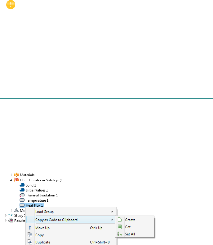
The

get, set, and create methods (described in the previous section) are also

accessible from the model tree by right-clicking and selecting

Copy as Code to

Clipboard

THE GET METHODS

The family of get methods is used to retrieve the values of properties. For

example, the

getDouble method can be used to retrieve the value of the

predefined element size property

hauto for a mesh and store it in a variable hv:

double hv = model.mesh("mesh1").feature("size").getDouble("hauto")

30 |

See the section “Example Code” on page 32 below for more information on the

property

hauto.

The syntax for the family of get methods for the basic data types is summarized in

the following table:

All arrays are returned as copies of the data; writing to a retrieved array does not

change the data in the model object. To change the contents of an array in the

model object, use one of the methods

set or setIndex.

Automatic type conversion is attempted from the property type to the requested

return type.

THE SET METHOD

The syntax for assignment using the set method is exemplified by this line of

code, which sets the title of a plot group

pg1:

model.result("pg1").set("title", "Temperature T in Kelvin");

The first argument is a string with the name of the property, in the above example

"title". The second argument is the value and can be a basic type as indicated by

the table below.

TYPE SYNTAX

String

getString(String name)

String array

getStringArray(String name)

String matrix

getStringMatrix(String name)

Integer

getInt(String name)

Integer array

getIntArray(String name)

Integer matrix

getIntMatrix(String name)

Double

getDouble(String name)

Double array

getDoubleArray(String name)

Double matrix

getDoubleMatrix(String name)

Boolean

getBoolean(String name)

Boolean array

getBooleanArray(String name)

Boolean matrix

getBooleanMatrix(String name)

TYPE SYNTAX

String

set(String name,String val1)

String array

set(String name,new String[]{"val1","val2"})

String matrix

set(String name,new String[][]{{"1","2"},{"3","4"}})

| 31

Using the set method for an object returns the object itself. This allows you to

append multiple calls to

set as follows:

model.result("pg1").set("edgecolor", "black").set("edges", "on");

The previous line of code assigns values to both the edgecolor and edges

properties of the plot group

pg1 and is equivalent to the two lines:

model.result("pg1").set("edgecolor", "black");

model.result("pg1").set("edges", "on");

In this case, the set method returns a plot group object.

Automatic type conversion is attempted from the input value type to the property

type. For example, consider a model parameter

a that is just a decimal number

with no unit. Its value can be set with the statement:

model.param().set("a", "7.54");

where the value "7" is a string. In this case, the following syntax is also valid:

model.param().set("a",7.54);

THE SETINDEX METHOD

The setIndex method is used to assign a value to a 1D or 2D array element at a

position given by one or two indices (starting from index 0).

The following line illustrates using

setIndex with one index:

model.physics("c").feature("cfeq1").setIndex("f", "2.5", 0);

The following line illustrates using setIndex with two indices:

model.physics("c").feature("cfeq1").setIndex("c", "-0.1", 0, 1);

For the setIndex method in general, use one of these alternatives to set the value

of a single element:

setIndex(String name,String value,int index);

setIndex(String name,String value,int index1,int index2);

Integer

set(String name,17)

Integer array

set(String name,new int[]{1,2})

Integer matrix

set(String name,new int[][]{{1,2},{3,4}})

Double

set(String name,1.3)

Double array

set(String name,new double[]{1.3,2.3})

Double matrix

set(String name,new double[][]{{1.3,2.3},{3.3,4.3}})

Boolean

set(String name,true)

Boolean array

set(String name,new boolean[]{true,false})

Boolean matrix

set(String name,new boolean[][]{{true, false},{false, false}})

TYPE SYNTAX

32 |

The name argument is a string with the name of the property. The value argument

is a string representation of the value. The indices start at 0, for example:

setIndex(name,value,2)

sets the third element of the property name to value.

The

setIndex method returns an object of the same type, which means that

setIndex methods can be appended just like the set method.

If the index points beyond the current size of the array, then the array is extended

as needed before the element at

index is set. The values of any newly created

intermediate elements are undefined.

The method

setIndex and set can both be used to assign values in ragged arrays.

For example, consider a ragged array with 2 rows. The code statements:

setIndex(name,{"1","2","3"},0);

setIndex(name,{"4","5"},1);

sets the first and second row of the array and are equivalent to the single statement:

set("name",new String[][]{{"1","2","3"},{"4","5"}});

METHODS ASSOCIATED WITH SET AND GET METHODS

For object types for which the set, setIndex, and get methods can be used, the

following additional methods are available:

String[] properties();

returns the names of all available properties,

boolean hasProperty(String name);

returns true if the feature has the named property,

String[] getAllowedPropertyValues(String name);

returns the allowed values for named properties, if it is a finite set.

EXAMPLE CODE

The following code block can be used to warn an application’s user of excessive

simulation times based on the element size:

if (model.mesh("mesh1").feature("size").getDouble("hauto")<=3) {

exp_time = "Solution times may be more than 10 minutes for finer element

sizes.";

}

In the above example, getDouble is used to retrieve the value of the property

hauto, which corresponds to the Element Size parameter Predefined in the Settings

window of the

Size node under the Mesh node. This setting is available when the

Sequence type is set to User-controlled mesh, in the Settings window of the Mesh

node.

| 33

The following line of code retrieves an array of strings corresponding to the

legends of a 1D point graph.

String[] legends =

model.results("pg3").feature("ptgr1").getStringArray("legends");

The figure below shows an example of a vector of legends in the Settings window

of the corresponding

Point Graph.

The following line of code sets the

Data Set dset1 for the Plot Group pg1:

model.result("pg1").set("data", "dset1");

The following lines of code set the anisotropic diffusion coefficient for a Poisson’s

equation problem on a block geometry.

model.geom("geom1").create("blk1", "Block");

with(model.geom("geom1").feature("blk1"));

set("size", new String[]{"10", "1", "1"});

endwith();

model.geom("geom1").run();

with(model.physics("c").feature("cfeq1"));

setIndex("c", "-0.1", 0, 1);

setIndex("c", "-0.2", 0, 6);

setIndex("f", "2.5", 0);

endwith();

The code below sets the global parameter L to a fixed value.

with(model.param());

set("L", "10[cm]");

endwith();

The code below sets the material link index to the string variable alloy, defined

under the

Declarations node.

with(model.material("matlnk1"));

set("link", alloy);

endwith();

The code below sets the coordinates of a cut point data set cpt1 to the values of

the 1D array

samplecoords[].

with(model.result().dataset("cpt1"));

set("pointx", samplecoords[0]);

34 |

set("pointy", samplecoords[1]);

set("pointz", samplecoords[2]);

endwith();

The code below sets the components of a deformation plot.

with(model.result("pg7").feature("surf1").feature("def"));

setIndex("expr", withstru, 0);

setIndex("expr", withstrv, 1);

setIndex("expr", withstrw, 2);

endwith();

The code below sets the title and color legend of a plot group pg2 and then

regenerates the plot.

with(model.result("pg2"));

set("titletype", "auto");

endwith();

with(model.result("pg2").feature("surf1"));

set("colorlegend", "on");

endwith();

model.result("pg2").run();

Parameters and Variables

This code defines a global parameter L with Expression 0.5[m] and Description

Length:

model.param().set("L", "0.5[m]");

model.param().descr("L", "Length");

There is an alternative syntax using three input arguments:

model.param().set("L", "0.5[m]", "Length");

You can also use the with syntax to set the Expression and Description for several

parameters, for example:

with(model.param());

set("L", "0.5[m]");

descr("L", "Length");

set("wd", "10[cm]");

descr("wd", "Width");

set("T0", "500[K]");

descr("T0", "Temperature");

endwith();

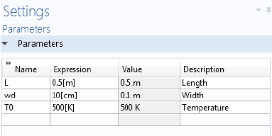
| 35

which corresponds to the following Settings window for Global

Definitions>Parameters

ACCESSING A GLOBAL PARAMETER

You would typically use the Editor Tools window for generating code for setting

the value of a global parameter. While in the Method editor, right-click the

parameter and select

Set.

To set the value of the global parameter

L to 10 cm:

model.param().set("L", "10[cm]");

To get the global parameter L and store it in a double variable Length:

double Length=model.param().evaluate("L");

The evaluation is in this case with respect to the base Unit System defined in the

model tree root node.

To return the unit of the parameter

L, if any, use:

String Lunit=model.param().evaluateUnit("L");

To write the value of a model expression to a global parameter, you typically need

to convert it to a string. The reason is that model expressions may contain units.

Multiply the value of the variable

Length with 2 and write the result to the

parameter

L including the unit of cm.

Length=2*Length;

model.param().set("L", toString(Length)+"[cm]");

To return the value of a parameter in a different unit than the base Unit System,

use:

double Length_real = model.param().evaluate("L","cm");

For the case where the parameter is complex valued, the real and imaginary parts

can be returned as a double vector of length 2:

double[] realImag = model.param().evaluateComplex("Ex","V/m");

For parameters that are numbers without units, you can use a version of the set

method that accepts a double instead of a string. For example, the lines

36 |

double a_double=7.65;

model.param().set(“a_param”,a_double);

assigns the value 7.65 to the parameter a_param.

VARIABLES

The syntax for accessing and assigning variables is similar to that of parameters.

For example, the code:

with(model.variable("var1"));

set("F", "150[N]");

descr("F", "Force");

endwith();

assigns the Expression 150[N] to the variable with Name F.

The following code assigns a model expression to the variable

with(model.variable("var1"));

set("f", "(1-alpha)^2/(alpha^3+epsilon)+1");

endwith();

and the following code stores the model expression for the same variable in a string

fs.

String fs = model.variable("var1").get("f");

Unary and Binary Operators in the Model Object

The table below describes the unary and binary operators that can be used when

accessing a model object, such as the model expressions used when defining

parameters, variables, material properties, and boundary conditions, as well as in

expressions used in results for postprocessing and visualization.

PRECEDENCE LEVEL SYMBOL DESCRIPTION

1 () {} . grouping, lists, scope

2 ^ power

3 ! - + unary: logical not, minus, plus

4 [] unit

5 * / binary: multiplication, division

6 + - binary: addition, subtraction

7 < <= > >= comparisons: less-than, less-than or equal,

greater-than, greater-than or equal

8 == != comparisons: equal, not equal

9 && logical and

| 37

The following example code creates a variable to indicate whether the effective von

Mises stress exceeds 200 MPa by using the inequality

solid.mises>200[MPa]:

model.variable().create("var1");

model.variable("var1").model("comp1");

model.variable("var1").set("hi_stress", "solid.mises>200[MPa]");

The following code demonstrates using this variable in a surface plot:

model.result().create("pg3", "PlotGroup3D");

model.result("pg3").create("surf1", "Surface");

with(model.result("pg3").feature("surf1"));

set("expr", "hi_stress");

endwith();

model.result("pg3").run();

The same plot can be created by directly using the inequality expression in the

surface plot expression as follows:

with(model.result("pg3").feature("surf1"));

set("expr", "solid.mises>200[MPa]");

endwith();

model.result("pg3").run();

Geometry

Once the Geometry node is created (see “Creating Model Components and Model

Object Nodes” on page 28) you can add geometric features to the node. For

example, add a square using default position (0, 0) and default size 1:

model.geom("geom1").create("sq1", "Square");

The first input argument "sq1" to the create method is a tag, a handle, to the

square. The second argument

"Square" is the type of geometry object.

Add another square with a different position and size:

model.geom("geom1").create("sq2", "Square");

with(model.geom("geom1").feature("sq2"));

set("pos", new String[]{"0.5", "0.5"});

set("size", "0.9");

endwith();

The with statement in the above example is used to make the code more compact

and, without using

with, the code statements above are equivalent to:

model.geom("geom1").feature("sq2").set("pos", new String[]{"0.5", "0.5"});

model.geom("geom1").feature("sq2").set("size", "0.9");

10 || logical or

11 , element separator in lists

PRECEDENCE LEVEL SYMBOL DESCRIPTION

38 |

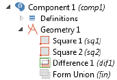
Take the set difference between the first and second square:

model.geom("geom1").create("dif1", "Difference");

with(model.geom("geom1").feature("dif1").selection("input"));

set(new String[]{"sq1"});

endwith();

with(model.geom("geom1").feature("dif1").selection("input2"));

set(new String[]{"sq2"});

endwith();

To build the entire geometry, you call the method run for the Geometry node:

model.geom("geom1").run();

The above example corresponds to the following Geometry node settings:

In this way, you have access to the functionality that is available in the geometry

node of the model tree. Use

Record Code or any of the other tools for automatic

generation of code to learn more about the syntax and methods for other

geometry operations.

REMOVING MODEL TREE NODES

You can remove geometry objects using the remove method:

model.geom("geom1").feature().remove("sq2");

Remove a series of geometry objects (circles) with tags c1, c2, ..., c10:

for(int n=1;n<=10;n=n+1) {

model.geom("geom1").feature().remove("c"+n);

}

The syntax "c"+n automatically converts the integer n to a string before

concatenating it to the string

"c".

To remove all geometry objects:

for(String tag : model.geom("geom1").feature().tags()) {

model.geom("geom1").feature().remove(tag);

}

However, the same can be achieved with the shorter:

model.geom("geom1").feature().clear();

In a similar way, you can remove other model tree nodes.

| 39

Mesh

The following line adds a Mesh node, with tag mesh1, linked to the geometry with

tag

geom1:

model.mesh().create("mesh1", "geom1");

You can control the mesh element size either by a preconfigured set of sizes or by

giving low-level input arguments to the meshing algorithm.

The following line:

model.mesh("mesh1").autoMeshSize(6);

corresponds to a mesh with Element size set to Coarse. The argument to the

method

autoMeshSize ranges from 1-9, where 1 is Extremely fine and 9 is

Extremely coarse.

To generate the mesh, you call the

run method for the mesh node:

model.mesh("mesh1").run();

Use Record Code to generate code for other mesh operations.

The code below shows an example where the global mesh parameters have been

changed.

model.mesh("mesh1").automatic(false); // Turn off Physics-controlled mesh

with(model.mesh("mesh1").feature("size"));

set("custom", "on"); // Use custom element size

set("hmax", "0.09"); // Maximum element size

set("hmin", "3.0E-3"); // Minimum element size

set("hgrad", "1.2"); // Maximum element growth rate

set("hcurve", "0.35"); // Curvature factor

set("hnarrow", "1.5"); // Resolution of narrow regions

endwith();

model.mesh("mesh1").run();

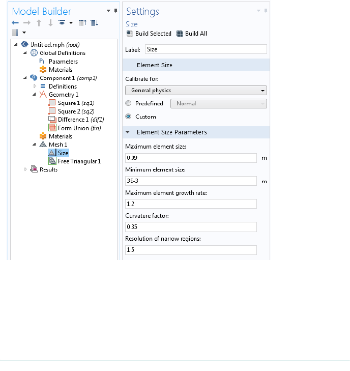
40 |

The above example corresponds to the following Mesh node settings:

Note that you can also set local element size properties for individual points,

edges, faces, and domains. Use

Record Code or any of the other tools for automatic

generation of code to learn more about the syntax and methods for other mesh

operations.

Physics

Consider analyzing stationary heat transfer in the solid rectangular geometry

shown earlier. To create a physics interface, for

Heat Transfer in Solids, use:

model.physics().create("ht", "HeatTransfer", "geom1");

The first input argument to the create method is a physics interface tag that is

used as a handle to this physics interface. The second input argument is the type

of physics interface. The third input argument is the tag of the geometry to which

the physics interface is assigned.

To set a fixed temperature boundary condition on a boundary, you first create a

TemperatureBoundary feature using the following syntax:

| 41

model.physics("ht").create("temp1", "TemperatureBoundary", 1);

The first input argument to create is a feature tag that is used as a handle to this

boundary condition. The second input argument is the type of boundary

condition. The third input argument is the spatial dimension for the geometric

entity that this boundary condition should be assigned to. Building on the

previous example of creating a 2D rectangle, the input argument being 1 means

that the dimension of this boundary is 1 (that is, an edge boundary in 2D).

The next step is to define which selection of boundaries this boundary condition

should be assigned to. To assign it to boundary 1 use:

model.physics("ht").feature("temp1").selection().set(new int[]{1});

To assign it to multiple boundaries, for example 1 and 3, use:

model.physics("ht").feature("temp1").selection().set(new int[]{1,3});

To set the temperature on the boundary to a fixed value of 400 K, use:

model.physics("ht").feature("temp1").set("T0", "400[K]");

The following lines of code show how to define a second boundary condition for

a spatially varying temperature, varying linearly with the coordinate

model.physics("ht").create("temp2", "TemperatureBoundary", 1);

model.physics("ht").feature("temp2").selection().set(new int[]{4});

model.physics("ht").feature("temp2").set("T0", "(300+10[1/m]*y)[K]");

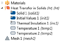
The resulting model tree structure is shown in the figure below.

Use

Record Code or any of the other tools for automatic generation of code to learn

more about the syntax and methods for other physics interface features and other

physics interfaces.

CREATING AND REMOVING MODEL TREE NODES

Below is a larger block of code that removes, creates, and accesses physics interface

feature nodes. It uses the

Iterator class and methods available in the java.util

package. For more information, see the Java

documentation.

String[] flowrate = column1;

String[] Mw = column2;

java.util.Iterator<PhysicsFeature> iterator =

model.physics(

"pfl").feature().iterator();

while (iterator.hasNext()) {

if (iterator.next().getType().equals(

"Inlet"))

42 |

iterator.remove();

}

if (flowrate != null) {

for (int i = 0; i < flowrate.length; i++) {

if (flowrate[i].length() > 0) {

if (Mw[i].length() > 0) {

int d = 1+i;

model.physics(

"pfl").create("inl"+d, "Inlet");

model.physics(

"pfl").feature("inl"+d).setIndex("spec", "3", 0);

model.physics(

"pfl").feature("inl"+d).set("qsccm0", flowrate[i]);

model.physics(

"pfl").feature("inl"+d).set("Mn", Mw[i]);

model.physics(

"pfl").feature("inl"+d).selection().set(new int[]{d});

}

The need to remove and create model tree nodes is fundamental when writing

methods because the state of the model object is changing each time a model tree

node is run. In the method above, the number of physics feature nodes are

dynamically changing depending on user inputs. Each time the simulation is run,

old nodes are removed first and then new nodes are added.

Material

A material, represented in the Model Builder by a Materials node, is a collection of

property groups, where each property group defines a set of material properties,

material functions, and model inputs that can be used to define, for example, a

temperature-dependent material property. A property group usually defines

properties used by a particular material model to compute a fundamental quantity.

To create a

Materials node:

model.material().create("mat1", "Common", "comp1");

You can give the material a name, for example, Aluminum, as follows:

model.material("mat1").label("Aluminum");

The following lines of code shows how to create a basic material property group

for heat transfer:

with(model.material("mat1").propertyGroup("def"));

set("thermalconductivity", new String[]{"238[W/(m*K)]"});

set("density", new String[]{"2700[kg/m^3]"});

set("heatcapacity", new String[]{"900[J/(kg*K)]"});

endwith();

| 43

The built-in property groups have a read-only tag. In the above example, the tag

def represents the property group Basic in the model tree.

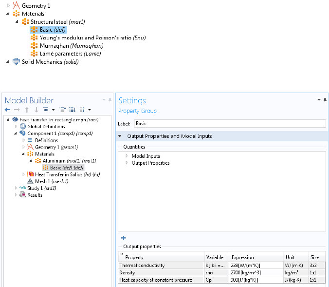
The resulting model tree and

Material node settings are shown in the figure below.

Note that some physics interfaces do not require a material to be defined. Instead,

the corresponding properties can be accessed directly in the physics interface. This

is also the case if the physics model settings are changed from

From material to User

defined

. For example, for the Heat Transfer in Solids interface, this setting can be

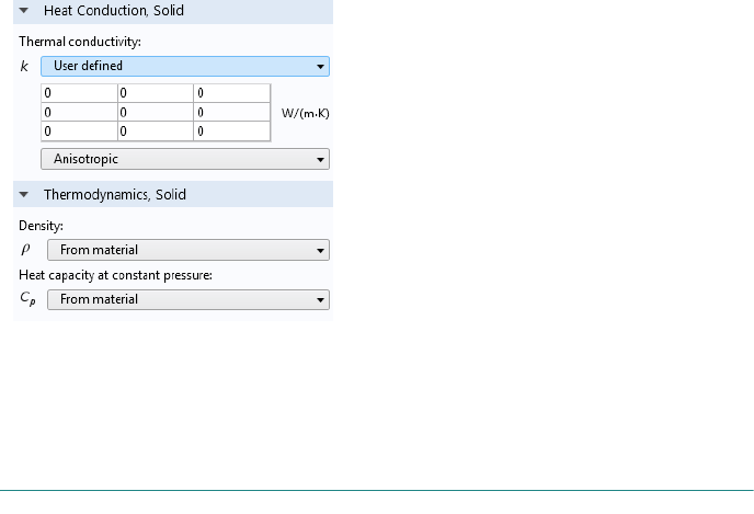
44 |

found in the Settings window of the subnode Solid, in the sections Heat Conduction,

Solid

and Thermodynamics, Solid, as shown in the figure below.

Use

Record Code or any of the other tools for automatic generation of code to learn

more about the syntax and methods for materials.

Study

The Study node in the model tree contains one or more study steps, instructions

that are used to set up solvers and solve for the dependent variables. The settings

for the

Study and the Solver Configurations nodes can be quite complicated.

Consider the simplest case for which you just need to create a study, add a study

step, and run it.

Building on the example from the previous sections regarding stationary heat

transfer, let’s add a

Stationary study step.

model.study().create("std1"); // Study with tag std1

model.study("std1").create("stat", "Stationary");

model.study("std1").run();

The call to the method run automatically generates a solver sequence in a data

structure

model.sol and then runs the corresponding solver. The settings for the

solver are automatically configured by the combination of physics interfaces you

have chosen. You can manually change these settings, as shown later in this

section. The data structure

model.sol roughly corresponds to the contents of the

Solver Configurations node under the Study node in the model tree.

All low-level solver settings are available in

model.sol. The structure

model.study is used as a high-level instruction indicating which settings should

be created in

model.sol when a new solver sequence is created.

| 45

For backward compatibility, some of the low-level settings in model.sol are

automatically generated when using

Record Code.

The example below shows a somewhat more elaborate case of programing the

study that would be applicable for the stationary heat transfer example shown

earlier. The instructions below more closely resemble the output autogenerated by

using the

Record Code option.

First create instances of the

Study node (with tag std1) and a Stationary study step

subnode:

model.study().create("std1");

model.study("std1").create("stat", "Stationary");

The actual settings that determine how the study is run are contained in a

sequence of operations in the

Solution data structure, with tag sol1, which is

linked to the study:

model.sol().create("sol1");

model.sol("sol1").study("std1");

The following code defines the sequence of operations contained in sol1.

First, create a

Compile Equations node under the Solution node to determine which

study and study step will be used:

model.sol("sol1").create("st1", "StudyStep");

model.sol("sol1").feature("st1").set("study", "std1");

model.sol("sol1").feature("st1").set("studystep", "stat");

Next, create a Dependent Variables node, which controls the scaling and initial

values of the dependent variables and determines how to handle variables that are

not solved for:

model.sol("sol1").create("v1", "Variables");

Now create a Stationary Solver node. The Stationary Solver contains the

instructions that are used to solve the system of equations and compute the values

of the dependent variables.

model.sol("sol1").create("s1", "Stationary");

Add subnodes to the Stationary Solver node to choose specific solver types. In this

example, use an

Iterative solver:

model.sol("sol1").feature("s1").create("i1", "Iterative");

Add a Multigrid preconditioner subnode:

model.sol("sol1").feature("s1").feature("i1").create("mg1", "Multigrid");

You can have multiple Solution data structures in a study node (such as sol1, sol2,

and so on) defining different sequences of operations. The process of notifying the

study of which one to use is done by “attaching” the

Solution data structure sol1

with study

std1:

model.sol("sol1").attach("std1");

46 |

The attachment step determines which Solution data structure sequence of

operations should be run when selecting

Compute in the COMSOL Desktop user

interface.

Finally, run the study, which is equivalent to running the

Solution data structure

sol1:

model.sol("sol1").runAll();

The resulting Study node structure is shown in the figure below. Note that there

are several additional nodes added automatically. These are default nodes and you

can edit each of these nodes by explicit method calls. You can edit any of the nodes

while using

Record Code to see the corresponding methods and syntax used.

MODIFYING LOW-LEVEL SOLVER SETTINGS

To illustrate how some of the low-level solver settings can be modified, consider

a case where the settings for the

Fully Coupled node are modified. This subnode

controls the type of nonlinear solver used.

| 47

The first line below may not be needed depending on whether the Fully Coupled

subnode has already been generated or not (it could have been automatically

generated by code similar to what was shown above).

model.sol("sol1").feature("s1").create("fc1", "FullyCoupled");

with(model.sol("sol1").feature("s1").feature("fc1"));

set("dtech", "auto"); // The Nonlinear method (Newton solver)

set("initstep", "0.01"); // Initial damping factor

set("minstep", "1.0E-6"); // Minimum damping factor

set("rstep", "10"); // Restriction for step-sized update

set("useminsteprecovery", "auto"); // Use recovery damping factor

set("minsteprecovery", "0.75"); // Recovery damping factor

set("ntermauto", "tol"); // Termination technique

set("maxiter", "50"); // Maximum number of iterations

set("ntolfact", "1"); // Tolerance factor

set("termonres", "auto"); // Termination criterion

set("reserrfact", "1000"); // Residual factor

endwith();

For more information on the meaning of these and other low-level solver settings,

see the Solver section of the Programming Reference Manual.

Changing the low-level solver settings requires that

model.sol has first been

created. It is always created the first time you compute a study, however, you can

trigger the automatic generation of

model.sol as follows:

model.study().create("std1");

model.study("std1").create("stat", "Stationary");

model.study("std1").showAutoSequences("sol");

where the call to showAutoSequences corresponds to the option Show Default

Solver

, which is available when right-clicking the Study node in the model tree.

This can be used if you do not want to take manual control over the settings in

model.sol (the solver sequence) and are prepared to rely on the physics interfaces

to generate the solver settings. If your application makes use of the automatically

generated solver settings, then updates and improvements to the solvers in future

versions are automatically included. Alternatively, the automatically generated

model.sol can be useful as a starting point for your own edits to the low-level

solver settings.

CHECKING IF A SOLUTION EXISTS

When creating an application it is often useful to keep track of whether a solution

exists or not. The method

model.sol("sol1").isEmpty() returns a boolean and

true if the solution structure sol1 is empty. Consider an application where the

solution state is stored in a string

solution_state. The following code sets the

state depending on the output from the

isEmpty method:

if (model.sol("sol1").isEmpty()) {

solution_state = "nosolution";

}

48 |

else {

solution_state = "solutionexists";

}

Almost all of the example applications in the Application Libraries use this

technique.

Results

The Results node contains nodes for Data Sets, Derived Values, Tables, Plot Groups,

Export, and Reports. As soon as a solution is obtained, a set of Plot Group nodes

are automatically created. In the example of

Heat Transfer in Solids, when setting

up such an analysis in the Model Builder, two

Plot Group nodes are added

automatically. The first one is a

Surface plot of the Temperature and the second one

is a

Contour plot showing the isothermal contours. Below you will see how to set

up the corresponding plots manually.

First create a 2D plot group with tag

pg1:

model.result().create("pg1", "PlotGroup2D");

Change the Label of the Plot Group:

model.result("pg1").label("Temperature (ht)");

Use the data set dset1 for the Plot Group:

model.result("pg1").set("data", "dset1");

Create a Surface plot for pg1 with settings for the color table used, the

intra-element interpolation scheme, and the data set referring to the parent of the

Surface plot node, which is the pg1 node:

model.result("pg1").feature().create("surf1", "Surface");

model.result("pg1").feature("surf1").label("Surface");

with(model.result("pg1").feature("surf1"));

set("colortable", "ThermalLight");

set("smooth", "internal");

set("data", "parent");

endwith();

Now create a second 2D plot group with contours for the isotherms:

model.result().create("pg2", "PlotGroup2D");

model.result("pg2").label("Isothermal Contours (ht)");

with(model.result("pg2"));

set("data", "dset1");

endwith();

model.result("pg2").feature().create("con1", "Contour");

model.result("pg2").feature("con1").label("Contour");

with(model.result("pg2").feature("con1"));

set("colortable", "ThermalLight");

set("smooth", "internal");

| 49

set("data", "parent");

endwith();

Finally, generate the plot for the Plot Group pg1:

model.result("pg1").run();

To find the maximum temperature, add a Surface Maximum subnode to the Derived

Values

node as follows:

First create the

Surface Maximum node with tag max1:

model.result().numerical().create("max1", "MaxSurface");

Note that in this context the method corresponding to the Derived Values node is

called

numerical.

Next, specify the selection. In this case there is only one domain 1:

model.result().numerical("max1").selection().set(new int[]{1});

Create a Table node to hold the numerical result and write the output from max1

to the

Table:

model.result().table().create("tbl1", "Table");

model.result().table("tbl1").comments("Surface Maximum 1 {max1} (T)");

model.result().numerical("max1").set("table", "tbl1");

model.result().numerical("max1").setResult();

Use Record Code or any of the other tools for automatic generation of code to learn

more about the syntax and methods for

Results.

Using Parameterized Solutions in Results

The code below changes the visualization of a plot group pg1 by setting the

property

looplevel, which controls the solution parameter, to the string variable

svar.

with(model.result("pg1"));

set("looplevel", new String[]{svar});

endwith();

model.result("pg1").run();

The property looplevel has a central role in accessing parameterized solutions.

Its argument is a 1D string array with one index per

"loop level" in a study. The

different loop levels correspond to the different nested parameters in a parametric

sweep with multiple parameters.

Loading Data to Tables

By using the loadFile method you can import data into a table and then display

it using a results table form object or a table surface plot. The following example

demonstrates loading data from an Excel file into a table and visualizing the

contents using a table surface plot. The file in this example is assumed to be

imported, in an application, using a file import form object with a file declaration

file1 as the File Destination.

50 |

model.result().table("tbl1").loadFile("upload:///file1", "", cells);

The string variable cells contains the spreadsheet selection to be

imported, for example A1:J7.

The following code creates a plot group pg1 with a table surface plot.

This code is not needed if the embedded model already contains a table

and a table surface plot.

model.result().create("pg1", 2);

model.result("pg1").create("tbls1", "TableSurface");

with(model.result("pg1").feature("tbls1"));

set("table", "tbl1");

endwith();

with(model.result("pg1").feature("tbls1"));

set("dataformat", "cells");

endwith();

model.result("pg1").feature("tbls1").create("hght1", "TableHeight");

with(model.result("pg1").feature("tbls1").feature("hght1"));

set("view", "view3");

endwith();

with(model.view("view3").camera());

set("viewscaletype", "manual");

set("xscale", "1");

set("yscale", "1");

set("zscale", "1");

endwith();

// The following line is needed to update the plot

model.result("pg1").run();

Multiphysics

Some of the physics interfaces define a multiphysics analysis by themselves without

being coupled to any other interface. This is the case when the physics interface is

used for a coupling that is so strong that it doesn’t easily lend itself to be separated

into several physics interfaces. In other cases, a set of single physics interfaces,

typically two, can be combined by the use of the

Multiphysics node. For example,

Joule Heating analysis is defined as the combination of an Electric Currents

interface and a

Heat Transfer in Solids interface with an additional Electromagnetic

Heat Source

node under the Multiphysics node. The following lines of code

illustrate the corresponding method calls.

model.physics().create("ec", "ConductiveMedia", "geom1");

model.physics().create("ht", "HeatTransfer", "geom1");

model.multiphysics().create("emh1", "ElectromagneticHeatSource", "geom1",

2);

model.multiphysics("emh1").selection().all();

with(model.multiphysics("emh1"));

| 51

set("EMHeat_physics", "ec");

set("Heat_physics", "ht");

endwith();

When using the Model Builder to set up a Joule Heating analysis, nodes in addition

to those shown above will be created corresponding to Joule heating in thin shells,

should they exist in the model, and temperature couplings if there are multiple

field variables for electric potential and temperature.

Working with Model Objects

When using the Model Builder in the COMSOL Desktop, an embedded model

with variable name

model is automatically created. The embedded model has a

special status. For example, the automatic code generation tools only consider the

embedded model. In addition, when you save to or load from an MPH file, only

the embedded model is saved or loaded. General tools include the

Save Application

command in the Application Builder and File > Save As, from the File menu of

the COMSOL Desktop environment.

However, in an application you are allowed to create and edit multiple models.

Saving and loading such models is done by using the built-in methods

saveModel

and

loadModel. An MPH file can only contain a single model object.

If you need to create model objects, in addition to the embedded model, use the

built-in method

createModel.

To create a new model you use:

Model extmodel = createModel();

A unique model tag is created automatically and assigned to the model. If you

want to explicitly control the model tag, use:

Model extmodel = createModel("My_model_1");

where My_model_1 is a unique tag. It is recommended that you do not use the

names

Model1, Model2, Model3, and so on, since these names are used by the

mechanism that automatically generates model tags for the embedded model

when loading and saving MPH files.

The following example retrieves the model tag of the embedded model:

String my_modeltag = model.tag();

however, you rarely need to use the model tag of the embedded model object.

Instead of creating and building up the contents of a model from scratch, you can

load an existing model and edit it.

For example in the Windows operating system, load a model

my_model.mph from

the folder

C:\COMSOL_Work, by using the built-in method loadModel:

52 |

Model extmodel = loadModel("C:\\COMSOL_Work\\my_model.mph");

A unique model tag is created automatically and is assigned to the model upon

load. Note the double-backslash syntax in the file name. Backslash (\) is a special

character in Java and the double backslash is needed in this case.

To make your application portable, you can use the file scheme syntax available in

the Application Builder. Assuming you stored the MPH file in the

common folder,

the call to

loadModel should be:

Model extmodel = loadModel("My_Model_1", "common:///my_model.mph");

In this example, the tag My_Model_1 is important since it is used to retrieve the

model from other methods. Once loaded, the model

extmodel exists in the work

space of the current COMSOL Multiphysics or COMSOL Server session. Note

that an MPH file can only contain one model object, so there is no ambiguity on

which model you refer to when loading an MPH file.

Assume that you, in one method, have loaded the model

extmodel with the tag

My_Model_1, such as in the example above. The model variable extmodel is not

available in other methods. In order to retrieve the model from another method

use:

Model mymodel = getModel("MyModel_1");

The contents of mymodel and extmodel are the same, but these variables exist in

the variable space of two different methods.

The tag

My_Model_1 uniquely identified and retrieved the model object from the

current COMSOL Multiphysics or COMSOL Server session.

To clear the contents of a model object, use the built-in method

clearModel.

For a list of model utility methods, see “Model Utility Methods” on page 91.

TURNING OFF AND RESET THE MODEL HISTORY

When running method code in applications or otherwise in order to automate

modeling tasks, the stored model history may become excessively large. The

model history is used, for example, when saving to Model M-file or Model

Java-file. Because of this, depending on the repetitive nature of your code, you

may need to temporarily turn off model history recording, as illustrated by the

following example:

model.hist().disable();

// some code

model.hist().enable();

If you wish to reset the model history to an almost minimal sequence of

commands that creates the current state of the model object you can use:

model.resetHist();

In the File menu, this functionality is referred to as Compact History.

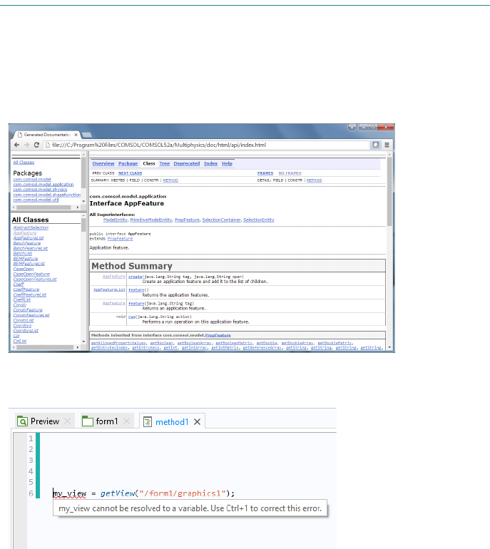
| 53

The Model Object Class Structure

For a full description of the class structure and method signatures, see the HTML

document Java Documentation available in the COMSOL Documentation. You

find the Java documentation under

COMSOL API for use with Java

at the bottom

of the Documentation window.

The figure below shows the document as displayed in a browser.

If you encounter a class that you are unfamiliar with you will get help by a tooltip

as in the figure below for the output of the

getView method.

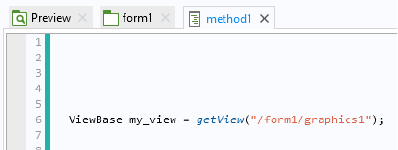
54 |

By using the keyboard shortcut Ctrl+1 the correct type declaration is assigned to

the variable as shown in the figure below.

This way you can avoid having to consult the Java Documentation.

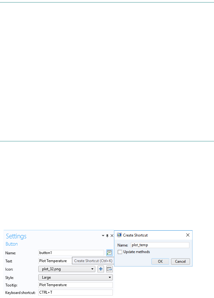
| 55

The Application Object

The application object is a part of the model object and is the data structure that

allows access to the user interface features of an application from within a method.

The state of the application object is reflected in the COMSOL Desktop user

interface by the contents of the Application Builder and its application tree.

You can write code using the Method editor to directly access and change the

features presented in a running application, including button text, icons, colors,

and fonts.

The application object gives you access to a subset of the features and settings

available in the Application Builder. You can use the application object methods

for run time modifications to the user interface, but not for building a complete

user interface. For building the user interface of an application, you need to use

the Form editor as described in the book Introduction to Application Builder.

This section gives an overview of the application object.

Shortcuts

Form objects and other user interface components are referenced in methods by

using a certain syntax. For example, using the default naming scheme

form3/button5 refers to a button with name button5 in form3 and

form2/graphics3 refers to a graphics object with name graphics3 in form2. You

can also change the default names of forms and form objects. For example, if

form1 is your main form then you can change its name to main.

To simplify referencing form objects as well as menu, ribbon, and toolbar items by

name, you can create shortcuts with a custom name. In the

Settings window of an

object or item, click the button to the right of the

Name field and type the name

of your choice.

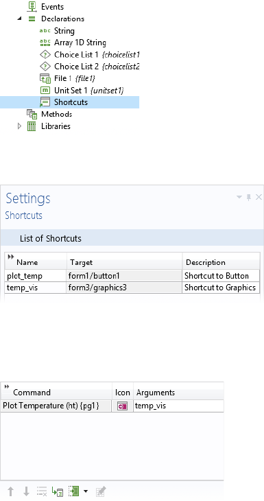
56 |

To create or edit a shortcut, you can also use the keyboard shortcut Ctrl+K.

All shortcuts that you create are made available in a

Shortcuts node under

Declarations in the application tree.

In the

Settings window for Shortcuts shown below, two shortcuts plot_temp and

temp_vis were created for a button and a graphics object, respectively.

The shortcuts can be referenced in other form objects or in code in the Method

editor. The example below shows a shortcut

temp_vis used as an input argument

to a temperature plot.

Shortcuts are automatically updated when objects are renamed, moved, copied,

and duplicated. They are available in application methods as read-only Java

variables, similar to string, integer, double, and Boolean declarations.

Using shortcuts is recommended because it avoids the need to update methods

when the structure of the application user interface changes.

Shortcuts can also be created for most objects in the model builder tree.

| 57

EXAMPLE CODE

If the application contains a button named button1 in a form named form1, and

the button has a shortcut named

b1, the following two ways to change the button

text to red are equivalent:

b1.set("foreground", "red");

app.form("form1").formObject("button1").set("foreground", "red");

Accessing the Application Object

In the Method editor you can directly access the application object part of the

model object by using the

app variable. This variable is a shorthand for

model.app().

The Name of User Interface Components

Access the various parts of the application object by using the name of a form

object, form, item, etc. A name in the application object has the same function as

the tag

in the model object omitting the model.app part.

For example, in the line of code

app.form("form1").formObject("button1").set("enabled", false);

the string form1 is the name of a form and button1 is the name of a button.

Important Classes

HE MAIN APPLICATION CLASS

When working with an application object, the main application class is AppModel,

which is the type of

model.app().

DECLARATION CLASSES

In addition to the basic data types and shortcut declarations, the Declaration node

may include Choice List and Unit List declarations. The corresponding classes are

ChoiceList and UnitSet. The parent class to ChoiceList and UnitSet is called

DataSource. In addition, Scalar, Array 1D, and Array 2D data types are handled

by the

DataSource class. For more information, see “Data Source” on page 84.

58 |

METHOD CLASS

The Method class is used to represent methods. For more information, see

“Method Class” on page 89.

MAIN USER INTERFACE COMPONENT CLASSES

In an application object, the main user interface components correspond to the

following classes:

• MainWindow

- The class representing the Main Window node in the application tree.

• Form

- The class representing a form.

• FormObject

- The class representing a form object.

• Item

- The class representing, for example, a menu, toolbar, or ribbon item.

Each class has a set of associated methods that are used to edit the corresponding

user interface component at run time. These are described in the following

sections.

In addition to the main user interface component classes, there are also list

versions of the

Form, FormObject, and Item classes. These are: FormList,

FormObjectList, and ItemList.

Get and Set Methods for the Color of a Form Object

The get and set methods described in the section “Get and Set Methods for

Accessing Properties” on page 29 are applicable to the model object as well as the

model.app part of the model object. In addition, the following methods are

available for changing the color of a form object:

NAME SYNTAX DESCRIPTION

setColor setColor(String prop, int r, int g, int b)

Set a color property using

red, green, and blue values.

getColor int[] getColor(String prop)

Get the value of a color

property as an array of red,

green, and blue values.

| 59

Not all methods are applicable to all properties. Use Ctrl+Space to use code

completion to find out what methods are applicable for a certain object, and what

property names and property values are applicable for a certain method.

General Properties

The following table lists properties that are available for several different user

interface components, including form objects. In the table below, a user interface

component is referred to as an object.

A foreground or background color property is represented by a string value. The

available colors are:

black, blue, cyan, gray, green, magenta, red, white, and

yellow, or a custom color may also be defined. The special value default means

PROPERTY VALUE DEFAULT DESCRIPTION

visible true | false true

If the value is true, the corresponding

object is visible in the user interface.

enabled true | false true

If the value is true, the

corresponding object is enabled in

the user interface, which means that

the user can interact with the object.

background String default

The background color for the

corresponding user interface element.

foreground String default

The foreground color for the

corresponding user interface element.

font String default

The font family name. The special

value default means that the font to

use is determined by the parent

object, which is the corresponding

setting in the Settings window of the

Forms node.

fontbold true | false false

If true the font uses boldface style.

fontitalic true | false false

If true the font uses italic style.

fontunderline true | false false

If true the font uses underline style.

fontsize String -1

The font size in points. The special

value

-1 represents the default size,

which means that the size is taken

from the parent object (the Forms

node) or from the system default size

if no parent object defines the size.

60 |

that the color is taken from the parent object. Depending on the parent type, this

could mean that

default is Inherit or Transparent, referring to the corresponding

setting in the

Settings window in the Form editor. An arbitrary RGB color can be

represented by a string of the form

rgb(red,green,blue) where red, green, and

blue are integers between 0 and 255. Color properties can also be manipulated

using the

getColor and setColor methods to directly access the red, green, and

blue color components. If a color property has the value

default, it does not have

red, green, and blue values. In this case, the

getColor method returns the array

[0,0,0].

EXAMPLE CODE

The following example reads the current background color for a form, makes the

color darker, and applies the modified color to the same form.

int[] rgb = app.form("form1").getColor("background");

for (int i = 0; i < 3; i++)

rgb[i] /= 2;

app.form("form1").setColor("background", rgb[0], rgb[1], rgb[2]);

The following line of code sets the background color to black:

app.form("form1").set("background", "black");

The following line of code sets the background color to default which in the case

of the background color property corresponds to the Form editor setting

Transparent.

app.form("form1").set("background", "default");

The following line of code sets the background color to the RGB values 125, 45,

and

43.

app.form("form1").set("background", "rgb(125,45,43)");

The Main Application Methods

The main application class AppModel has the following methods:

NAME SYNTAX DESCRIPTION

mainWindow MainWindow mainWindow()

Returns the MainWindow object.

form FormList form()

Returns the list of forms.

form Form form(String name)

Returns the form with the specified name.

| 61

The AppModel class has the following properties:

EXAMPLE CODE

app.set("asktosave", true);

The following code appends a text string to the application window title.

String oldTitle = app.mainWindow().getString("title");

app.mainWindow().set("title", oldTitle+" modified");

Main Window

The MainWindow class has the following methods:

declaration DataSource

declaration(String name)

Returns the declaration object (Scalar, Array 1D,

Array 2D, ChoiceList, or UnitSet) with the

specified name.

hasProperty boolean hasProperty(String

name)

Returns true if there is a modifiable property with

the specified name.

PROPERTY VALUE DEFAULT DESCRIPTION

asktosave true | false false

If true, ask user if changes should be saved before

the application is closed.

startmode edit | run edit

Determines whether the application is opened

for editing or running when you double-click the

MPH file, including Windows desktop icons.

NAME SYNTAX DESCRIPTION

menuBar ItemList menuBar()

Returns the list of items in the menu bar.

menuBar Item menuBar(String

name)

Returns the menu bar item with the specified

name.

toolBar ItemList toolBar()

Returns the list of items in the toolbar.

toolBar Item toolBar(String

name)

Returns the toolbar item with the specified name.

ribbon ItemList ribbon()

Returns the list of items in the ribbon.

ribbon Item ribbon(String name)

Returns the ribbon item with the specified name.

fileMenu ItemList fileMenu()

Returns the list of items in the file menu.

NAME SYNTAX DESCRIPTION

62 |

The menuBar and toolBar items are visible in the application user interface if the

menu type is set to

Menu bar in the Settings window of the Main Window. The

ribbon and

fileMenu items are visible in the user interface if the menu type is set

Ribbon. It is possible to access and modify items that are not visible based on

the menu type setting, but doing so will not have any visible effect in the user

interface.

The

MainWindow class has the following properties:

EXAMPLE CODE

app.mainWindow().set("showfilename", false);

Form

The Form class has the following methods:

fileMenu Item fileMenu(String

name)

Returns the file menu item with the specified

name.

hasProperty boolean

hasProperty(String name)

Returns true if there is a modifiable property with

the specified name.

PROPERTY VALUE DEFAULT DESCRIPTION

showfilename true

| false true

If true the filename is included in the

window title bar title.

title String My application

The text to display in the window

title bar.

NAME SYNTAX DESCRIPTION

getName String getName()

Returns the name of this

form.

getParentForm Form getParentForm()

Returns the parent form that

contains this form. Useful for

local cards in a card stack.

formObject FormObjectList formObject()

Returns the list of form

objects.

formObject FormObject formObject(String name)

Returns the form object with

the specified name.

NAME SYNTAX DESCRIPTION

| 63

The Form class has the following properties:

EXAMPLE CODE

app.form("form1").set("icon", "compute.png");

app.form("form1").formObject("button1").set("enabled", false);

DataSource ds = app.form("form1").declaration("var");

Form Object

The FormObject class has the following methods:

hasProperty boolean hasProperty(String name)

Returns true if there is a

modifiable property with the

specified name.

declaration DataSource declaration(String name)

Returns a form declaration

object (Scalar, Array 1D,

Array 2D, or ChoiceList) with

the specified name.

method MethodList method()

Returns the list of methods.

method Method method(String name)

Gets a method with the

specified name.

PROPERTY VALUE DEFAULT DESCRIPTION

icon String

The name of the background image.

Valid values are images defined in

Images>Libraries node in the

application tree.

iconhalign left | center |

right | fill |

repeat

center

Horizontal alignment for the

background image.

iconvalign top | center |

bottom | fill |

repeat

center

Vertical alignment for the background

image.

title String Form N

The form title for an integer N.

NAME SYNTAX DESCRIPTION

getName String getName()

Returns the name of this form object.

getParentForm Form getParentForm()

Returns the parent form that contains this form

object.

NAME SYNTAX DESCRIPTION

64 |

Most form objects have one or more of the properties listed in “General

Properties” on page 59. A form object has a certain property if the corresponding

setting is available in the Form editor. Additional properties are supported for

several types of form objects. The general properties that are supported and any

additional properties for form objects are listed in the following sections.

EXAMPLE CODE

The following code loops over all buttons and disables them:

for (FormObject formObject : app.form("form1").formObject()) {

if ("Button".equals(formObject.getType())) {

formObject.set("enabled", false);

}

The getType method retrieves the type of form object. In the above example the

type of form object is Button and the statement

"Button".equals(formObject.getType()) represents a string comparison

between the output of the

getType method and the string "Button".

The following table lists all form object types that can be returned by

getType:

getType String getType()

Returns the form object type name, as defined in

the following sections.

form FormList form()

For a CardStack form object, returns the list of

local cards.

form Form form(String name)

For a CardStack form object, returns the local card

with the specified name.

item ItemList item()

For a Toolbar, Graphics or Table form object,

returns the list of user-defined buttons.

item Item item(String name)

For a Toolbar, Graphics or Table form object,

return the user-defined button with the specified

name.

hasProperty boolean

hasProperty(String

name)

Returns true if there is a modifiable property with

the specified name.

FORM OBJECT TYPE

ArrayInput Hyperlink SelectionInput

Button Image Slider

CardStack InformationCardStack Spacer

CheckBox InputField Table

ComboBox Line Text

NAME SYNTAX DESCRIPTION

| 65

ARRAY INPUT

Example Code

app.form("form1").formObject("arrayinput1").set("enabled", false);

BUTTON

In the Form editor, if a button has its Size setting set to Large, it always displays its

text property. If the button is Small, it either displays the icon or the text

DataDisplay ListBox TextLabel

Equation Log ToggleButton

FileImport MessageLog Toolbar

Form ProgressBar Unit

FormCollection RadioButton Video

Graphics ResultsTable WebPage

Property Value Default Description

background

enabled

font

fontbold

fontitalic

fontsize

foreground

visible

See “General Properties” on page 59.

PROPERTY VALUE DEFAULT DESCRIPTION

enabled

font

fontbold

fontitalic

fontsize

foreground

visible

See “General Properties” on page 59.

icon String

The button icon. Valid values are

images defined in

"Images > Libraries"

in the Application Builder.

text String

Generated

automatically

The button text. The text must not be

an empty string.

tooltip String

The button tooltip text.

FORM OBJECT TYPE

66 |

according to the following rule: if the icon property is empty, the text is

displayed, if the

icon property is not empty, the icon is displayed.

Example Code

app.form("form1").formObject("button1").set("enabled", false);

CARD STACK

Example Code

app.form("form1").formObject("cardstack1").set("visible", false);

To access objects in a local card, either use shortcuts or use the form method:

app.form("form1").formObject("cardstack1").form("card1").formObject("butto

n1").set("enabled", false);

CHECK BOX

Example Code

app.form("form1").formObject("checkbox1").set("tooltip", "tooltip text");

PROPERTY VALUE DEFAULT DESCRIPTION

enabled

visible

See “General Properties” on

page 59.

PROPERTY VALUE DEFAULT DESCRIPTION

background

enabled

font

fontbold

fontitalic

fontsize

fontunderline

foreground

visible

See “General Properties” on

page 59.

text String

Generated

automatically

The check box label text.

tooltip String

The check box tooltip text.

| 67

COMBO BOX

Example Code

app.form("form1").formObject("combobox1").set("foreground", "blue");

PROPERTY VALUE DEFAULT DESCRIPTION

enabled

font

fontbold

fontitalic

fontsize

foreground

visible

See “General Properties” on

page 59.

68 |

DATA DISPLAY

Example Code

app.form("form1").formObject("datadisplay1").setColor("background", 192,

192, 192);

PROPERTY VALUE DEFAULT DESCRIPTION

background

enabled

font

fontbold

fontitalic

fontsize

foreground

visible

See “General Properties” on

page 59.

exponent superscript | E superscript

When set to superscript,

exponents are displayed using

superscript font. When set to

exponents are displayed using

the character

E followed by the

exponent value.

notation auto |

scientific |

decimal

auto

When the value is scientific,

numbers are always displayed

using scientific notation. When

the value is

decimal, numbers

are never displayed using

scientific notation. When the

value is

auto, the notation

depends on the size of the

number.

precision Integer 4

The number of significant digits

that are displayed.

showunit true | false true

Controls if the unit is displayed

in addition to numerical values.

tooltip String

The tooltip text.

| 69

EQUATION

Example Code

app.form("form1").formObject("equation1").set("visible", false);

FILE IMPORT

Example Code

app.form("form1").formObject("fileimport1").set("filetypes", new

String[]{"ALL2DCAD"});

FORM

A form used as a subform does not have any modifiable properties.

PROPERTY VALUE DEFAULT DESCRIPTION

enabled

fontsize

foreground

visible

See “General Properties” on

page 59.

equation

String The string in LaTeX syntax

defining the equation.

PROPERTY VALUE DEFAULT DESCRIPTION

background

enabled

font

fontbold

fontitalic

fontsize

foreground

visible

See “General Properties” on page 59.

buttontext String Browse...

Text to display on the button that opens

the file browser.

dialogtitle String File import

Text to display as dialog title for the file

browser dialog. Also displayed as a tooltip

for the

FileBrowser form object.

filetypes String[] {"ALLFILES"}

Defines the list of file types that can be

selected in the file browser.

70 |

FORM COLLECTION

To modify the active pane, change the corresponding declaration variable.

Example Code

This line of code changes the font:

app.form("form1").formObject("collection1").set("font", "Arial");

The expanded state of sections in form collections can be controlled by:

app.form("form1").formObject("formcollection1").expanded("form2", false);

The expanded method is only supported by form collections which use sections.

The first argument is the tag of the form which is represented by the section. The

second argument determines if the sections should be expanded or collapsed.

GRAPHICS

Example Code

This line of code displays plot group 5 (pg5) in the graphics object graphics1 in

the form with the name

Temperature:

app.form("Temperature").formObject("graphics1").set("source",

model.result("pg5"));

PROPERTY VALUE DEFAULT DESCRIPTION

enabled

font

fontbold

fontitalic

fontsize

foreground

visible

See “General Properties” on page 59.

PROPERTY VALUE DEFAULT DESCRIPTION

enabled

visible

See “General Properties” on page 59.

datapick true | false false

If true, data picking is enabled in the

graphics form object.

datapicktarget ProbeFeature |

GraphicsData

Defines where the picked data is

stored. Valid values are probe features

and GraphicsData declarations.

source ModelEntity

Defines the type of model entity (Plot

Group, Geometry, Mesh, Explicit

Selection or Player Animation) used

to plot in the graphics form object.

| 71

The following line of code using useGraphics is equivalent to the above example:

useGraphics(model.result("pg5"), "Temperature/graphics1");

Either method changes the source of the graphics form object and then plots the

contents.

To clear the contents of a graphics object, use:

app.form("Temperature").formObject("graphics1").set("source",

(ModelEntity) null);

or equivalently

useGraphics(null, "Temperature/graphics1");

The code below displays the mesh in the model tree node mesh1 in the graphics

object

graphics1 contained in the card of a card stack:

app.form("mesh").formObject("cardstack1").form("card1").formObject("graphi

cs1").set("source", model.mesh("mesh1"));

The code below enables data picking for a graphics object and sets the data picking

target to a domain point probe:

app.form("form1").formObject("graphics1").set("datapick", true);

app.form("form1").formObject("graphics1").set("datapicktarget",

model.component("comp1").probe("pdom1"));

If a shortcut graphics1 has been created for the graphics object and a shortcut

pdom1 has been created for the probe object, the above can be shortened to:

graphics1.set("datapick", true);

graphics1.set("datapicktarget", pdom1);

HYPERLINK

Example Code

with (app.form("form1").formObject("hyperlink1"));

set("text", "COMSOL");

set("url", "www.comsol.com");

endwith();

PROPERTY VALUE DEFAULT DESCRIPTION

background

enabled

font

fontbold

fontitalic

fontsize

visible

See “General Properties” on page 59.

text String

Generated

automatically

The text to display on the HyperLink

form object.

url String

The URL to open when the HyperLink

is activated.

72 |

IMAGE

Example Code

app.form("form1").formObject("image1").set("icon", "compute.png");

INFORMATION CARD STACK

Example Code

app.form("form1").formObject("infocard1").set("fontunderline", true);

PROPERTY VALUE DEFAULT DESCRIPTION

enabled

visible

See “General Properties” on page 59.

icon String cube_large.png

Defines the icon name to display in the

Image form object. Valid values are

images defined in the Images>Libraries

node in the application tree.

PROPERTY VALUE DEFAULT DESCRIPTION

background

enabled

font

fontbold

fontitalic

fontsize

fontunderline

visible

See “General Properties” on page

59.

| 73

INPUT FIELD

PROPERTY VALUE DEFAULT DESCRIPTION

background

enabled

font

fontbold

fontitalic

fontsize

foreground

visible

See “General Properties” on

page 59.

editable true | false true

If true then the text in the input

field can be edited by the user.

exponent superscript | E superscript

When set to superscript,

exponents are displayed using

superscript font. When set to E,

exponents are displayed using

the character

E followed by the

exponent value.

inputformatting on | off off

If the value is on, then numerical

values in the input field are

formatted according to the

exponent, notation and

precision properties. When the

user is editing the text in the

input field, the formatting is

temporarily disabled so that the

original text can be edited.

maxdouble

double

1000

The maximum allowed double

value. This property is only

accessible when the Filter setting

is set to Double and the

corresponding check box is

enabled in the Data Validation

section.

mindouble

double

The minimum allowed double

value. This property is only

accessible when the Filter setting

is set to Double and the

corresponding check box is

enabled in the Data Validation

section.

74 |

Example Code

app.form("form1").formObject("inputfield1").set("precision", 6);

maxinteger Integer 1000

The maximum allowed integer

value. This property is only

accessible when the Filter setting

is set to Integer and the

corresponding check box is

enabled in the Data Validation

section.

mininteger Integer 0

The minimum allowed integer

value. This property is only

accessible when the Filter setting

is set to Integer and the

corresponding check box is

enabled in the Data Validation

section.

notation auto |

scientific |

decimal

auto

When the value is scientific,

numbers are always displayed

using scientific notation. When

the value is

decimal, numbers

are never displayed using

scientific notation. When the

value is

auto, the notation

depends on the size of the

number.

precision Integer 4

The number of significant digits

displayed.

tooltip String

The tooltip displayed when the

mouse pointer is located over

the input field.

PROPERTY VALUE DEFAULT DESCRIPTION

| 75

LINE

Example Code

app.form("form1").formObject("line1").set("text", "divider text");

app.form("form1").formObject("line1").set("thickness", 10);

app.form("form1").formObject("line1").set("linecolor", blue);

LIST BOX

Example Code

app.form("form1").formObject("listbox1").set("foreground", "red");

To change the list box contents, modify the corresponding choice list:

app.declaration("choicelist1").appendListRow("new value", "new name");

PROPERTY VALUE DEFAULT DESCRIPTION

enabled

font

fontbold

fontitalic

fontsize

foreground

visible

See “General Properties” on page 59.

text String

Text to display on the line. The text is only

displayed for horizontal lines that have Include

divider text enabled in the Line object Settings

window.

thickness Integer

The line thickness.

linecolor String

default

The line color.

PROPERTY VALUE DEFAULT DESCRIPTION

enabled

font

fontbold

fontitalic

fontsize

foreground

visible

See “General Properties” on page 59.

76 |

LOG

Example Code

app.form("form1").formObject("log1").set("fontsize", "20");

MESSAGE LOG

Example Code

app.form("form1").formObject("messages1").set("background", "gray");

PROGRESS BAR

To create and update progress information see “Progress Methods” on page 125.

Example Code

app.form("form1").formObject("progressbar1").set("visible", false);

PROPERTY VALUE DEFAULT DESCRIPTION

background

enabled

font

fontbold

fontitalic

fontsize

foreground

visible

See “General Properties” on page 59.

PROPERTY VALUE DEFAULT DESCRIPTION

background

enabled

font

fontbold

fontitalic

fontsize

foreground

visible

See “General Properties” on page 59.

PROPERTY VALUE DEFAULT DESCRIPTION

enabled

visible

See “General Properties” on page 59.

| 77

RADIO BUTTON

To change the display name for a radio button, modify the value in the

corresponding choice list.

For a choice list that is used by a radio button, it is not possible to change the value

of any row, or to add or remove rows. Only the display name can be changed.

Example Code

app.form("form1").formObject("radiobutton1").set("fontitalic", true);

app.declaration("choicelist1").setDisplayName("new name", 0);

RESULTS TABLE

To change the contents of the results table use the method useResultsTable or

evaluateToResultsTable. See also “GUI-Related Methods” on page 111.

Example Code

app.form("form1").formObject("resultstable1").set("visible", true);

app.form(“form1”).formObject(“resultstable1”).set(“source”,

model.result().table("tbl2"));

useResultsTable(model.result().table("tbl2"), "/form1/resultstable1");

PROPERTY VALUE DEFAULT DESCRIPTION

background

enabled

font

fontbold

fontitalic

fontsize

fontunderline

foreground

visible

See “General Properties” on page 59.

PROPERTY VALUE DEFAULT DESCRIPTION

enabled

font

fontbold

fontitalic

fontsize

foreground

visible

See “General Properties” on page 59.

source

TableFeature Set the contents of the results table.

78 |

SELECTION INPUT

Example Code

app.form("form1").formObject("selectioninput1").set("graphics",

"graphics1");

Alternatively, if there are shortcuts sel1 and g1 to the selectioninput1 and

graphics1 form objects:

sel1.set("graphics", g1);

To change the model selection, assuming sel1 is a shortcut to the selection input

form object:

sel1.set("source", model.selection("sel2"));

PROPERTY VALUE DEFAULT DESCRIPTION

background

enabled

font

fontbold

fontitalic

fontsize

foreground

visible

See “General Properties” on page 59.

graphics FormObject

Defines the graphics form object to

use when the selection form object is

active.

source SelectionFeature

Defines the model selection the

selection form object is connected to.

| 79

SLIDER

The min value is allowed to be larger than the max value, in which case the slider

behaves as if the values were swapped. The smallest value always corresponds to

the left side of the slider.

Example Code

app.form("form1").formObject("slider1").set("min", 1);

app.form("form1").formObject("slider1").set("max", 12);

app.form("form1").formObject("slider1").set("steps", 11);

SPACER

A spacer object does not have any modifiable properties.

PROPERTY VALUE DEFAULT DESCRIPTION

enabled

visible

See “General Properties” on page 59.

max double 1

The largest possible slider value.

min double 0

The smallest possible slider value.

steps integer 5

The number of steps between the min and

max values. The number of tick marks is one

more than the number of steps.

tooltip String

The tooltip text.

type real | integer real

If type has the value integer, then the slider

value is restricted to integer values. If

type

has the value

real, the slider value can be a

noninteger value.

80 |

TABLE

To change the contents of the table, change the declaration variables or model

entities the table is displaying.

Example Code

app.form("form1").formObject("table1").set("enabled", false);

TEXT

Example Code

app.form("form1").formObject("text1").set("textalign", "center");

PROPERTY VALUE DEFAULT DESCRIPTION

enabled

font

fontbold

fontitalic

fontsize

foreground

visible

See “General Properties” on page 59.

headers

String[]

Generated

automatically

Column headers.

showheaders

boolean

Generated

automatically

Show column headers.

PROPERTY VALUE DEFAULT DESCRIPTION

background

enabled

font

fontbold

fontitalic

fontsize

foreground

visible

See “General Properties” on page 59.

editable on | off off

If the value is on, the text can be

edited by the user of the application. If

the value is

off, the text can only be

changed programmatically.

textalign left | center |

right

left

Defines how the text is aligned within

the text area.

wrap on | off on

If the value is on, word wrapping is

used to break lines that are too long

to fit within the text area. If the value

off, long lines may not be

completely visible.

| 81

TEXT LABEL

Example Code

app.form("form1").formObject("textlabel1").set("text", "custom text");

TOGGLE BUTTON

A button with size large always displays the text, a button with size small displays

either the icon or the text. If the icon property is empty, the text is displayed. If

the icon property is not empty, the icon is displayed.

Example Code

app.form("form1").formObject("togglebutton1").set("icon",

"about_information.png");

PROPERTY VALUE DEFAULT DESCRIPTION

background

enabled

font

fontbold

fontitalic

fontsize

fontunderline

foreground

visible

See “General Properties” on

page 59.

text String

Generated

automatically

The text to display in the

label when the label is not in

multiline mode.

textmulti String

Generated

automatically

The text to display in the

label when the label is in

multiline mode.

PROPERTY VALUE DEFAULT DESCRIPTION

enabled

font

fontbold

fontitalic

fontsize

foreground

visible

See “General Properties” on page 59.

icon String

The button icon. Valid values are images

defined in

"Images>Libraries" in the

Application Builder.

text String

Generated

automatically

The button text. The text must not be

an empty string.

tooltip String

The button tooltip text.

82 |

TOOLBAR

Example Code

app.form("form1").formObject("toolbar1").set("background", "gray");

UNIT

Example Code

app.form("form1").formObject("unit1").set("visible", false);

VIDEO

Example Code

app.form("form1").formObject("video1").set("visible", false);

PROPERTY VALUE DEFAULT DESCRIPTION

background

enabled

font

fontbold

fontitalic

fontsize

foreground

visible

See “General Properties” on page 59.

PROPERTY VALUE DEFAULT DESCRIPTION

background

enabled

font

fontbold

fontitalic

fontsize

foreground

visible

See “General Properties” on page 59.

PROPERTY VALUE DEFAULT DESCRIPTION

visible

See “General

Properties” on page 59.

| 83

WEB PAGE

Example Code

app.form("form1").formObject("webpage1").set("type", "report");

app.form("form1").formObject("webpage1").set("report", "rpt1"));

model.result().report("rpt1"));

model.result().report("rpt1").run();

Item

Item objects represent items, toggle items, user defined buttons in Toolbar,

Graphics and Table form objects, and submenus in the menu bar, toolbar, ribbon

and file menu. The following methods are available:

PROPERTY VALUE DEFAULT DESCRIPTION

visible

See “General Properties” on

page 59.

file

String The file to display. File scheme

syntax is supported.

html

String

The HTML code to display.

report

ReportFeature

or String

The report feature to display.

type page | url |

type | report

page

Determines which property is

used to specify the browser

display contents.

url

String

http://www.comsol.com

The URL to display.

NAME SYNTAX DESCRIPTION

item ItemList item()

Returns the list of subitems.

item Item item(String name)

Returns the subitem with the specified name.

getParentItem Item getParentItem()

Returns the parent item, or null for a

top-level item.

hasProperty boolean

hasProperty(String

name)

Returns true if there is a modifiable property

with the specified name.

84 |

The Item class contains the following properties:

In order for an item to be enabled, the

enabled property needs to have the value

on for the item itself as well as for all of its parents. In other words, disabling an

item also disables all of its subitems.

Item objects also include separators. However, separators do not have any

accessible properties.

Item objects for user-defined buttons do not have the

title and tooltip

properties. For Table form objects, predefined items such as “move up” and

“move down” do not have any modifiable properties.

EXAMPLE CODE

app.mainWindow().menuBar("menu1").set("title", "new title");

app.mainWindow().menuBar("menu1").item("toggle_item1").set("text",

"test");

Data Source

A DataSource object is either a Scalar, Array 1D, Array 2D, ChoiceList a

UnitSet or a GraphicsData.

PROPERTY VALUE DEFAULT DESCRIPTION

enabled on | off on

If the value is on, the item can be activated

by the user. If the value is

off, the item

cannot be activated.

icon

String Generated

automatically

The icon name. Valid values are images

defined in Images > Libraries in the

Application Builder.

text

String Generated

automatically

The text for a menu or ribbon item.

title

String Generated

automatically

The title text for a menu or submenu.

tooltip

String

The tooltip text.

visible on | off on

Controls whether the item is visible or not.

| 85

SCALAR, ARRAY 1D, AND ARRAY 2D METHODS

The methods described in the following table are applicable for Scalar, Array 1D,

and

Array 2D objects (of types String, Boolean, Integer, Double). These

methods are used to manipulate such variable objects during run time.

NAME SYNTAX DESCRIPTION

getBoolean boolean getBoolean()

Gets the Boolean value stored in

the data source.

getBooleanArray boolean[] getBooleanArray()

Gets the Boolean array value

stored in the data source.

getBooleanMatrix boolean[][] getBooleanMatrix()

Gets the Boolean matrix value

stored in the data source.

getDouble double getDouble()

Gets the double value stored in

the data source.

getDoubleArray double[] getDoubleArray()

Gets the double array value

stored in the data source.

getDoubleMatrix double[][] getDoubleMatrix()

Gets the double matrix value

stored in the data source.

getInt int getInt()

Gets the int value stored in the

data source.

getIntArray int[] getIntArray()

Gets the int array value stored in

the data source.

getIntMatrix int[][] getIntMatrix()

Gets the int matrix value stored

in the data source.

getString String getString()

Gets the String value stored in

the data source.

getStringArray String[] geStringArray()

Gets the String array value stored

in the data source.

getStringMatrix String[][] getStringMatrix()

Gets the String matrix value

stored in the data source.

set set(boolean value)

set(boolean[] value)

set(boolean[][] value)

set(double[] value)

set(double[][] value)

set(int value)

set(int[] value)

set(int[][] value)

set(String value)

set(String[] value)

set(String[][] value)

Set the value stored in the data

source. Available methods

depend on the type of the

underlying declaration.

86 |

EXAMPLE CODE

// Get a scalar double declaration.

DataSource ds = app.declaration("var");

// The 'var' declaration is a scalar double so we use the getDouble method

// to read its value.

double cur = ds.getDouble();

// Modifying the local field 'cur' doesn't affect the value stored in the

// data source 'ds'.

cur = cur + 1;

// Set the value of the data source.

ds.set(cur);

CHOICE LIST AND UNIT SET METHODS

The methods described in the following table are applicable for both ChoiceList

and

UnitSet objects. These methods are used to manipulate choice lists and unit

sets during run time.

NAME SYNTAX DESCRIPTION

setListRow setListRow(String value, String

displayName, int row)

Sets the value and display name

for the given row (0-based). If the

row is equal to the length of the

list, a new row is added.

setList setList(String[] values, String[]

displayNames)

Sets all of the values and display

names, replacing the contents of

the choice list or unit set.

setValue setValue(String value, int row)

Sets the value for the given row

(0-based). If the row is equal to

the length of the list, a new row is

added with the value and an

empty display name.

setDisplayName setDisplayName(String displayName, int

row)

Sets the display name for the

given row (0-based). If the row is

equal to the length of the list, a

new row is added with the

display name and an empty value.

getValue String getValue(int row)

Returns the value for the given

row (0-based).

getDisplayName String getDisplayName(int row)

Returns the display name for the

given row (0-based).

getDisplayName String getDisplayName(String value)

Returns the display name for the

row with the given value.

getValues String[] getValues()

Returns all values as an array.

| 87

Example Code

The code below adds the string Aluminum 3004 to a choice list. Note that the

choice list index starts at 0, whereas the material tags start at 1 (

mat1, mat2, mat3,

and

mat4).

ChoiceList choiceList = getChoiceList("choicelist1");

choiceList.setListRow("mat4", "Aluminum 3004", 3);

For more information on using choice lists for changing materials, see the book

Introduction to Application Builder.

UNIT SET METHODS

When the object is a UnitSet the following additional methods are also available:

GRAPHICSDATA METHODS

When the object is a GraphicsData the following methods are available:

getDisplayNames String[] getDisplayNames()

Returns all display names as an

array.

addListRow addListRow(String value, String

displayName, int row)

Inserts a new row with the given

value and display name at the

specified row (0-based).

appendListRow appendListRow(String value, String

displayName)

Inserts a new row with the given

value and display name at the end

of the list.

removeListRow removeListRow(int row)

Removes the given row (0-based)

from the list.

NAME SYNTAX DESCRIPTION

set set(String value)

Switch unit for the unit set.

getString String getString()

Returns the currently selected value for the unit

set.

getString String

getString(String

unitList)

Returns the selected unit for the given unit list.

NAME SYNTAX DESCRIPTION

set set(String name, String value)

set(String name, double value)

set(String name, double[] value)

Sets a new value for the property

with the specified name.

getString String getString(String name)

Returns the value of the specified

property as a string.

NAME SYNTAX DESCRIPTION

88 |

The GraphicsData class has the following properties:

Example code

The following code enables data picking for the graphics1 object, connects it to

the

graphicsdata1 object and sets some properties on the graphicsdata1 object:

app.form("form1").formObject("graphics1").set("datapick", true);

app.form("form1").formObject("graphics1").set("datapicktarget",

app.declaration("graphicsdata1"));

app.declaration("graphicsdata1").set("edim", "boundary");

app.declaration("graphicsdata1").set("method", "pointdir");

getDouble double getDouble(String name)

Returns the value of the specified

property as a double value.

getDoubleArray double[] getDoubleArray(String

name)

Returns the value of the specified

property as a double array value.

PROPERTY VALUE DEFAULT DESCRIPTION

coord

double[]

0, 0, 0

Point location of picked data. Array of

1, 2, 3 or 6 elements, corresponding

to 1D, 2D, 3D, or Smith plot,

respectively.

depth

double

Point along a line when data picking in

a domain. Valid values are between 0

and 1, inclusive.

edim

domain |

boundary

domain

Geometric entity level.

eval

double

Evaluated value of picked data.

method

pointnormal |

pointdir |

twopoints |

none

pointnormal

Method of selecting a point in a 3D

geometry.

twopoint

first | second

first

Point being picked in the twopoints

line entry method.

NAME SYNTAX DESCRIPTION

| 89

Method Class

The Method class is used to represent a method. The following method is available

for a

Method object:

The following code exemplifies using a

Method object:

// Get a Method object representing a Form Method.

Method m = app.form("form1").method("method1");

// The method takes a String parameter and returns a double.

double res = (Double) m.run("input");

Form, Form Object, and Item List Methods

The FormList, FormObjectList, and ItemList classes have the following

methods:

Additionally the FormList class has the following methods:

NAME SYNTAX DESCRIPTION

run Object run(Object... input)

Run the method with the specified

input parameters.

NAME SYNTAX PURPOSE

names String[] names()

Returns an array of names for all objects in the

list.

size int size()

Returns the number of objects in the list.

index int index(String name)

Returns the 0-based position of the object with a

given name in the list.

get Form get(String name)

FormObject get(String

name)

Item get(String name)

Returns the object with a given name.

get Form get(int index)

FormObject get(int

index)

Item get(int index)

Returns the object at a certain index.

NAME SYNTAX PURPOSE

hasProperty boolean

hasProperty(String name)

Returns true if there is a modifiable property with

the specified name.

90 |

It is also possible to use a list in an enhanced for loop to operate on all objects in

the list.

In the following example, the background color is set to red in all forms, by

looping over all forms:

for (Form f : app.form()) { // app.form() is of type FormList

f.set("background", "red");

}

| 91

The Built-in Method Library for the Application Builder

This section lists built-in methods available in the Method editor in addition to

the methods that operate on the model and application objects. For more

information on the model object and its methods, refer to earlier sections of this

book and the Programming Reference Manual. For more information on the

application object, see “The Application Object” on page 55. Some of the listings

have associated example code but for more extensive programming examples, see

“Programming Examples” on page 150.

The syntax rules are those of the Java

programming language. Note that each line

of code needs to end with a semicolon (

;), but the semicolon is omitted in the

listings below.

Model Utility Methods

The following table summarizes the model utility methods for querying, creating,

loading, and saving model objects. The model object is stored on the MPH file

format.

NAME SYNTAX DESCRIPTION

clearModel clearModel(Model model)

clearModel(String tag)

Remove everything from the

model except for the application

part and the things you can

change on the root node in the

Model Builder, such as thumbnail,

comment and author.

createModel Model createModel(String tag)

Creates a new model with the

given tag.

createModel Model createModel()

Create a new model with a

unique tag.

getModel Model getModel(String tag)

Returns the model with a

specified tag.

loadModel Model loadModel(String tag, String

filename)

Loads a model with a specified

tag from a file.

loadModel Model loadModel(String filename)

Loads a model from a file. The

model is given a unique tag.

loadProtectedModel Model loadProtectedModel(String tag,

String filename, String password)

Loads a password protected

model with a specified tag from a

file.

92 |

Example Code

The code below loads a model using loadModel, presented in the table above. It

extracts the x-, y-, and z-coordinates of all mesh nodes and stores them in a 2D

double array

coords[3][N], where N is the number of mesh nodes. The individual

x-,y-, and z- coordinates are available as the length-N 1D arrays

coords[0],

coords[1], coords[2], respectively. (The node locations can be plotted by using

the Cut Point 3D data set in combination with a 3D Point Trajectories plot.)

Model extmodel = loadModel("C:\\Paul\\pacemaker_electrode.mph");

SolverFeature step = extmodel.sol("sol1").feature("v1");

XmeshInfo xmi = step.xmeshInfo();

XmeshInfoNodes nodes = xmi.nodes();

double[][] coords = nodes.coords();

For more information on methods operating on the model object, see the

Programming Reference Manual.

Note that to make the code above platform independent for use in an application

you can instead use the common application file folder:

Model extmodel = loadModel("common:///pacemaker_electrode.mph");

loadProtectedModel Model loadProtectedModel(String

filename, String password)

Loads a password protected

model from a file. The model is

given a unique tag.

loadRecoveryModel Model loadRecoveryModel(String tag,

String foldername)

Loads a model from a recovery

directory/folder structure.

loadRecoveryModel Model loadRecoveryModel(String

foldername)

Loads a model from a recovery

directory/folder structure. The

model is given a unique tag.

modelTags String[] modelTags()

Returns an array of model tags

for all loaded models, including

the embedded model.

removeModel removeModel(String tag)

removeModel(Model model)

Removes a model. The

embedded model cannot be

removed.

saveModel saveModel(Model model, String

filename)

Saves a model to a file. The

filename can be a file scheme

path or (if allowed by security

settings) a server file path.

uniqueModeltag String uniqueModeltag(String prefix)

Returns a model tag that is not in

use.

getComsolVersion getComsolVersion()

Returns the current software

version as a string.

NAME SYNTAX DESCRIPTION

| 93

License Methods

The license methods read the license number and check out or test the licenses of

the current session or for an MPH file. This functionality can be used, for example,

to limit the use of an application to one or a few license numbers or to dynamically

adapt functionality of an application depending on which product licenses are

available.

NAME SYNTAX DESCRIPTION

checkoutLicense boolean checkoutLicense(String...

product)

Checks out licenses for all

specified products. If not all

licenses can be checked out, no

licenses are checked out.

checkoutLicenseFor

File

boolean checkoutLicenseForFile(String

file)

Checks out licenses required to

use a given MPH file. If not all

required licenses can be checked

out, no licenses are checked out.

checkoutLicenseFor

FileOnServer

boolean

hasLicenseForFileOnServer(String

file);

Checks out licenses required to

use a given MPH file. If not all

required licenses can be checked

out, no licenses are checked out.

getLicenseNumber String license = getLicenseNumber()

Returns a string with the license

number for the current session.

hasProduct boolean hasProduct(String... product)

Returns true if the COMSOL

installation contains the software

components required for running

the specified products. Code

completion can be used to get a

list of valid product names.

hasProductForFile boolean hasProductForFile(String file)

Returns true if the COMSOL

installation contains the software

components required for running

the products required by a given

MPH file.

hasProductForFileO

nServer

boolean

checkoutLicenseForFileOnServer(String

file);

Returns true if the COMSOL

installation contains the software

components required for running

the products required by a given

MPH file.

94 |

EXAMPLE CODE

The following code tries to check out a license for the AC/DC Module, and

displays an error message if it fails:

if (!checkoutLicense(“ACDC”))

alert(“There seems to be a problem. Please contact Alice and Bob at

123-456-7890.”);

You can use this to customize license error messages by calling a method

containing this code before any add-on product specific features are used by the

application.

In the Application Builder root node you can further select the

Ignore license errors

during launch

check box. This will make it possible for users to start an application

regardless of which licenses are available. However, this will not work if the

application, at startup, uses features required by an add-on product. The

application has to be created in such a way that the add-on product specific

features are not used in the start-up phase of the application but instead are

deferred to later in the work-flow.

To emulate a scenario where there are not enough available licenses you can, for

example, disable one or more products in the

Licensed and Used Products in Session

dialog box, available from the

File menu in the COMSOL Desktop environment.

The following code tests if the COMSOL installation has the capability to use an

MPH file:

boolean ok = hasProductForFile(“model_file.mph”);

Note that even if hasProductForFile return true, in a floating network license

situation there may not be any free licenses to check out. If your application is

going to process several MPH files and you want to make sure all licenses are

checked out before the processing starts, instead use the

checkoutLicense or

checkoutLicenseForFile methods.

LICENSE FEATURE STRINGS

The following table contains the product strings for all add-on products in the

COMSOL 5.5 product suite that can be used by the method

checkoutLicense:

PRODUCT/FEATURE FEATURE NAME

AC/DC Module ACDC

Acoustics Module ACOUSTICS

Batteries & Fuel Cells Module BATTERIESANDFUELCELLS

CAD Import Module CADIMPORT

CFD Module CFD

| 95

Chemical Reaction Engineering Module CHEM

Corrosion Module CORROSION

Design Module DESIGN, CADIMPORT

ECAD Import Module ECADIMPORT

Electrochemistry Module ELECTROCHEMISTRY

Electrodeposition Module ELECTRODEPOSITION

Fatigue Module FATIGUE

File Import for CATIA V5 CATIA5

Geomechanics Module GEOMECHANICS

Heat Transfer Module HEATTRANSFER

LiveLink™

for AutoCAD® LLAUTOCAD, CADIMPORT

LiveLink™

for PTC® Creo® Parametric™ LLCREOPARAMETRIC,

CADIMPORT

LiveLink™

for Excel® LLEXCEL

LiveLink™

for Inventor® LLINVENTOR, CADIMPORT

LiveLink™

for MATLAB® LLMATLAB

LiveLink™

for Revit® LLREVIT, CADIMPORT

LiveLink™

for PTC® Pro/ENGINEER® LLPROENGINEER, CADIMPORT

LiveLink™

for Solid Edge® LLSOLIDEDGE, CADIMPORT

LiveLink™

for SOLIDWORKS® LLSOLIDWORKS, CADIMPORT

Material Library MATLIB

MEMS Module MEMS

Metal Processing Module METALPROCESSING

Microfluidics Module MICROFLUIDICS

Mixer Module MIXER

Molecular Flow Module MOLECULARFLOW

Multibody Dynamics Module MULTIBODYDYNAMICS

Nonlinear Structural Materials Module NONLINEARSTRUCTMATERIALS

Optimization Module OPTIMIZATION

Particle Tracing Module PARTICLETRACING

Pipe Flow Module PIPEFLOW

Plasma Module PLASMA

Porous Media Flow Module POROUSMEDIAFLOW

PRODUCT/FEATURE FEATURE NAME

96 |

File Methods

File methods are used to read and write data to a file or portions of a file. Note

that higher-level techniques for reading and writing to files are available from

within the Application Builder user interface. For more information, see the book

Introduction to Application Builder and “GUI Command Methods” on page

122.

Ray Optics Module RAYOPTICS

RF Module RF

Rotordynamics Module ROTORDYNAMICS

Semiconductor Module SEMICONDUCTOR

Structural Mechanics Module STRUCTURALMECHANICS

Subsurface Flow Module SUBSURFACEFLOW

Wave Optics Module WAVEOPTICS

NAME SYNTAX DESCRIPTION

readFile String readFile(String name)

Returns the contents in the given

file name as a string. The string

name is the absolute path to a file

or a path given by the file scheme

syntax.

openFileStreamReader CsReader

openFileStreamReader(String

name)

Returns a CsReader that can be

used to read line-by-line or

character-by-character from the

given file

name.

openBinaryFileStreamReader CsBinaryReader

openBinaryFileStreamReader(Stri

ng name)

Returns a CsBinaryReader that

can be used to read from the

given file byte-by-byte.

readMatrixFromFile double[][]

readMatrixFromFile(String name)

Reads the contents of the given

file into a double matrix. The file

has the same spreadsheet type

format as available in the model

tree Export node.

PRODUCT/FEATURE FEATURE NAME

| 97

readStringMatrixFromFile String[][]

readStringMatrixFromFile(String

name)

Reads the contents of the given

file into a string matrix. The file

has the same spreadsheet type

format as available in the model

tree Export node.

readCSVFile String[][] readCSVFile(String

name)

Reads a file with

comma-separated values (CSV

file) into a string matrix. Expects

file to use the RFC 4180 format

for CSV.

writeFile writeFile(String name, String

contents)

Writes the given string contents

to the given file

name.

writeFile writeFile(String name, String

contents, boolean append)

Writes the given string contents

to the given file

name. If append is

true, then the contents are

appended instead of overwritten.

writeFile writeFile(String name,

double[][] data)

Writes the array data to the

given file. The spreadsheet format

is used, which means it can be

read by

readMatrixFromFile.

writeFile writeFile(String name,

double[][] data, boolean

append)

Writes the array data to the

given file. The spreadsheet format

is used, which means it can be

read by

readMatrixFromFile. If

append is true, then the contents

are appended instead of

overwritten.

writeFile writeFile(String name,

String[][] data)

Writes the array data to the

given file. The spreadsheet format

is used, which means it can be

read by

readStringMatrixFromFile.

writeFile writeFile(String name,

String[][] data, boolean

append)

Writes the array data to the

given file. The spreadsheet format

is used, which means it can be

read by

readStringMatrixFromFile. If

append is true, then the contents

are appended instead of

overwritten.

NAME SYNTAX DESCRIPTION

98 |

openFileStreamWriter CsWriter

openFileStreamWriter(String

name)

Returns a CsWriter that can

write to the given file.

openFileStreamWriter CsWriter

openFileStreamWriter(String

name, boolean append)

Returns a CsWriter that can

write to the given file. If

append is

true, then the contents are

appended instead of overwritten.

openBinaryFileStreamWriter CsBinaryWriter

openBinaryFileStreamWriter(Stri

ng name)

Returns a CsBinaryWriter that

can be used to write to the given

file byte-by-byte.

openBinaryFileStreamWriter CsBinaryWriter

openBinaryFileStreamWriter(Stri

ng name, boolean append)

Returns a CsBinaryWriter that

can be used to write to the given

file byte by byte. If

append is true,

then the contents are appended

instead of overwritten.

writeCSVFile writeCSVFile(String name,

String[][] data)

Writes the given string array

data to a CSV file. The RFC 4180

format is used for the CSV.

writeCSVFile writeCSVFile(String name,

String[][] data, boolean

append)

Writes the given string array

data to a CSV file. The RFC 4180

format is used for the CSV. If

append is true, then the contents

are appended instead of

overwritten.

writeCSVFile writeCSVFile(String name,

double[][] data)

Writes the given double array

data to a CSV file. The RFC 4180

format is used for the CSV.

writeCSVFile writeCSVFile(String name,

double[][] data, boolean

append)

Writes the given double array

data to a CSV file. The RFC 4180

format is used for the CSV. If

append is true, then the contents

are appended instead of

overwritten.

NAME SYNTAX DESCRIPTION

| 99

exists boolean exists(String name)

Tests whether a file with the given

name exists.

If the name is not a file scheme

path name or an absolute path,

then the method first finds out

whether a file with file scheme

path

embedded:/// + argument

exists. If such a file does not exist,

then it tests whether there is a

file with a matching

name in the

current working directory.

deleteFile deleteFile(String file)

Delete a file with the given name

if it exists. The file is deleted on

the server,. The name can use a

file scheme path.

copyFile copyFile(String sourceFile,

String destFile)

Copies a file on the server. Both

the source and target names can

use file scheme paths.

importFile importFile(String name)

importFile(String name,

String[] fileTypes)

Displays a file browser dialog box

and uploads the selected file to

the file declaration with the given

name. After this, the uploaded file

can be accessed with

upload:///<name>. The optional

fileTypes argument can be used

to filter which file types are

available for selection in the file

browser. The easiest way to get a

list of valid file types is to use

code completion in the method

editor.

NAME SYNTAX DESCRIPTION

100 |

importFile importFile(ModelEntity entity,

String name)

Displays a file browser dialog box

and uploads the selected file to

the Filename text field in the

given model object entity. This

defines an input file that the

application will need at a later

stage. For example, the Filename

of an interpolation function

accessed with

model.func(’<tag>’)). The

uploaded file can be accessed

with

upload:///<tag>/filename.

writeExcelFile writeExcelFile(String name,

String[][] data)

Writes the given string array

data starting from the first cell in

the first sheet of an Excel file.

This method requires LiveLink™

for

Excel

writeExcelFile writeExcelFile(String name,

String sheet, String cell,

String[][] data)

Writes the given string array

data starting from the specified

cell in the specified sheet of an

Excel file. This method requires

LiveLink™ for

Excel

readExcelFile String[][] readExcelFile(String

name)

Reads the first sheet of an Excel

file, starting from the first cell,

into a String[][]. This method

requires LiveLink™ for

Excel

readExcelFile String[][] readExcelFile(String

name, String sheet, String

cell)

Reads the specified sheet of an

Excel file, starting from the

specified cell, into a String[][].

This method requires LiveLink™

for

Excel

NAME SYNTAX DESCRIPTION

| 101

getFilePath String getFilePath(String name)

Returns the absolute server file

path of the server proxy file

corresponding to a certain file

scheme path, or null if the server

proxy file for the given path does

not exist.

This method can be used to pass

the path to, for example, a file

using the

temp:/// scheme to

external code or an application.

In addition, this method is used to

retrieve the file name of an

uploaded file when using the file

scheme

upload:///inputFile,

for example by using a File

declaration together with a File

Import form object.

getClientFileName String getClientFileName(String

name)

Returns the original name of an

uploaded file on the client file

system (or null if there is no

uploaded file matching the given

file scheme path).

This method is only useful for

providing user interface feedback.

For example, to get information

on which uploaded file is being

used. There is no guarantee that

the original file would still exist on

the client or even that the

current client would be the same

as the original client.

NAME SYNTAX DESCRIPTION

102 |

EXAMPLE CODE

This line of code copies the uploaded file file1 to the temp folder with new file

name

file2.mphbin and then prompts the user to save the file to a any location.

copyFile("upload:///file1", "temp:///file2.mphbin");

fileSaveAs("temp:///file2.mphbin");

This line of code deletes the file file2.mphbin from the temp folder.

deleteFile("temp:///file2.mphbin");

This line of code creates a directory in the user folder, as specified in Preferences.

createDirectory("user:///a/b");

This line of code creates a directory in the Temp folder under C:.

createDirectory("C:\\Temp\\a\\b");

getClientFilePath String getClientFilePath(String

name)

Returns the original path of an

uploaded file on the client file

system (or null if there is no

uploaded file matching the given

file scheme path). Returns only

the file name part of the path

when called from an application

running in a web browser.

This method is only useful for

providing user interface feedback.

For example, to get information

on which uploaded file is being

used. There is no guarantee that

the original file would still exist on

the client or even that the

current client would be the same

as the original client.

createDirectory createDirectory(String name)

Creates a file directory name, see

examples below in the Example

Code section.

NAME SYNTAX DESCRIPTION

| 103

Operating System Methods

Operating system methods are used for accessing operating system information

and commands from an application.

NAME SYNTAX DESCRIPTION

executeOSCommand String executeOSCommand(String

command, String... params)

Executes the OS command with

the given command (full path)

and parameters. Execution times

out after a default 180 seconds.

Returns everything the process

printed to its out stream as a

string. When applicable, the

command is run server side.

executeOSCommand String executeOSCommand(String

command, int timeoutSec, String

params...)

Executes the OS command with

the given command (full path)

and parameters. Returns

everything the process printed to

its out stream as a string. The

execution is forcibly stopped after

timeoutSec seconds if the

command has not finished. To

disable the timeout functionality,

timeoutSec value 0 can be used.

When applicable, the command

is run server side.

fileOpen fileOpen(String name)

Opens the file represented by

name with the associated

program on the client. Also see

the section “Example code”.

getUser String username = getUser()

Returns the username of the user

that is running the application. If

the application is not run from

COMSOL Server, then the value

of the preference setting

General>Username>Name is

returned.

openURL openURL(String url)

Opens a URL in the default

browser on the client.

104 |

EXAMPLE CODE

The line of code below plays one of the sounds available in the data/sounds folder

of the COMSOL installation and has been embedded in the application and stored

in the Sounds library.

playSound("embedded:///success_1.wav");

In the command sequence of a form object, this is equivalent to selecting a sound

node under

Libraries and clicking Run.

The line of code below opens a PDF file embedded in the application and stored

in the File library.

fileOpen("embedded:///tubular_reactor.pdf");

In the command sequence of a form object, this is equivalent to selecting an Open

File

node under GUI Commands>File Commands and clicking Run.

playSound playSound(String name)

Plays the sounds in the given file

on the client. Only

.wav files are

supported; no external libraries

are required.

playSound playSound(double hz, int millis)

Plays a signal at a given frequency

hz and with given duration

millis in milliseconds on the

client.

NAME SYNTAX DESCRIPTION

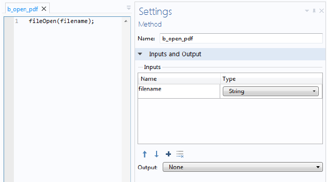
| 105

As an alternative technique, you can call a method in a command sequence with

an input argument, as shown in the example below. The figure below shows a

method

b_open_pdf that opens a file with filename as an input argument.

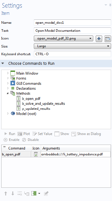
106 |

The figure below shows the corresponding command sequence for a ribbon menu

item.

Note that the same functionality is available from a command sequence by

selecting the editor tree node

GUI Commands>File Commands>Open File.

This line of code opens the COMSOL home page in the default browser:

openURL("http://www.comsol.com");

This line of code runs an application by means of an OS command:

executeOSCommand("C:\\COMSOL55\\Multiphysics\\bin\\win64\\comsol.exe",

"-run", "C:\\work\\tubular_reactor.mph");

| 107

Email Methods

Email methods are used for sending emails from an application, typically with

attachments containing results from a simulation.

Email Class Methods

The class EmailMessage can be used to create custom email messages.

NAME SYNTAX DESCRIPTION

emailFromAddress String emailFromAddress()

Returns the email from address

from the COMSOL Server or

preferences setting.

sendEmail sendEmail(String subject, String

bodyText)

Sends an email to the default

recipient(s) with the specified

subject and body text.

sendEmail sendEmail(String subject, String

bodyText, ModelEntity... modelEntity)

Sends an email to the default

recipient(s) with the specified

subject, body text, and zero or

more attachments created from

Report, Export, and Table nodes

in the embedded model.

sendEmail sendEmail(String toAddress, String

subject, String bodyText,

ModelEntity... modelEntity)

Sends an email to the specified

recipient(s) with the specified

subject, body text, and zero or

more attachments created from

Report, Export, and Table nodes

in the embedded model.

userEmailAddress String userEmailAddress()

Returns the user email

address(es) corresponding to the

currently logged in user, or an

empty string if the user has not

configured an email address.

NAME SYNTAX DESCRIPTION

EmailMessage EmailMessage mail = new EmailMessage()

Creates a new EmailMessage

object.

EmailMessage.setSer

ver

mail.setServer(String host, int port)

Sets the email (SMTP) server

host and port to use for this

email message.

108 |

EmailMessage.setUse

mail.setUser(String name, String

password)

Sets the username and password

to use for email (SMTP) server

authentication. This method must

be called after the

setServer

method.

EmailMessage.setSec

urity

mail.setSecurity(String security)

Sets the connection security type

for email (SMTP) server

communication. Valid values are

’none’, ’starttls’ and ’tls’.

This method must be called after

the setServer method.

EmailMessage.setFro

mail.setFrom(String fromAddress)

Sets the from address.

EmailMessage.setTo mail.setTo(String... to)

Sets the to addresses.

EmailMessage.setCc mail.setCc(String... cc)

Sets the cc addresses.

EmailMessage.setBcc mail.setBcc(String... bcc)

Sets the bcc addresses.

EmailMessage.setSub

ject

mail.setSubject(String subject)

Sets the email subject line. Note

that newline characters are not

allowed.

EmailMessage.setBod

yText

mail.setBodyText(String body)

Sets the email body as plain text.

An email can contain both a text

and an HTML body.

EmailMessage.setBod

yHtml

mail.setBodyHtml(String body)

Sets the email body as HTML

text. An email can contain both a

text and an HTML body.

EmailMessage.attach

File

mail.attachFile(String filename)

Adds an attachment from a file.

The attachment MIME type is

determined by the file name

extension.

EmailMessage.attach

File

mail.attachFile(String filename,

String mimeType)

Adds an attachment from a file

with the specified MIME type.

EmailMessage.attach

FromModel

mail.attachFromModel(ModelEntity

modelEntity)

Adds an attachment created

from a report, export, or table

feature in the model.

EmailMessage.attach

Text

mail.attachText(String text, String

mimeSubType)

Adds a text attachment with a

specified sub-MIME type, such as

plain or HTML.

NAME SYNTAX DESCRIPTION

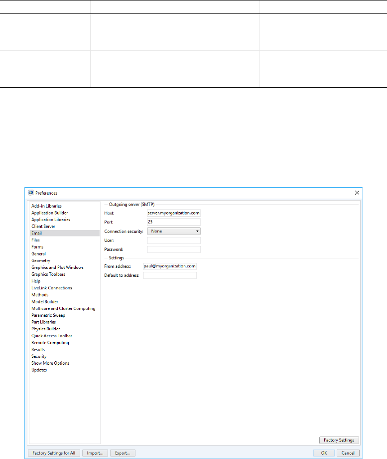
| 109

Each to, cc, and bcc address string can contain multiple email addresses separated

by a comma or a semicolon character. Whitespace is allowed before and after the

separator character.

EMAIL PREFERENCES

To set preferences for an outgoing email (SMTP) server, open the Email page of

the

Preferences dialog box, as shown in the figure below.

COMSOL Server provides a similar set of email preferences.

EmailMessage.attach

Binary

mail.attachBinary(byte[] binary,

String mimeType)

Adds an attachment from a byte

array with the specified MIME

type.

EmailMessage.send mail.send()

Sends the email to the email

(SMTP) server. An email object

can only be sent once.

NAME SYNTAX DESCRIPTION

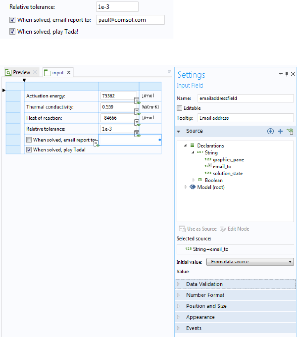
110 |

EXAMPLE CODE

The following code sends an email and attaches a report:

EmailMessage mail = new EmailMessage();

mail.setTo(email_to);

mail.setSubject("Tubular Reactor Simulation");

mail.setBodyText("The computation has finished. Please find the report

attached.");

mail.attachFromModel(model.result().report("rpt1"));

mail.send();

This code is run in the Tubular Reactor application, which is available as an

application example in the Application Libraries. The figure below shows part of

the user interface with an input field for the email address.

The figure below shows the corresponding form object and

Settings window.

The following code is similar but also configures the email server settings.

| 111

EmailMessage mail = new EmailMessage();

mail.setServer("smtp.myemail.com", 587);

mail.setUser("user@myemail.com", "password");

mail.setSecurity("starttls");

mail.setFrom("user@myemail.com");

mail.setTo("otheruser@somedomain.com");

mail.setSubject("Tubular reaction simulation");

mail.setBodyText("The computation has finished");

mail.send();

GUI-Related Methods

The graphical user interface (GUI) related methods are used for displaying dialog

boxes with messages, editing form objects and user interface content, getting

run-time properties of the application user interface, and running methods.

NAME SYNTAX DESCRIPTION

Call a method directly

<methodName>()

Call a method from the

Methods list by using its

name, for example,

method1(), method2().

callMethod callMethod(String name)

Alternate way to call a

method from the Methods

list; used internally and in

cases of name collisions.

useGraphics useGraphics(ModelEntity entity,

String name)

useGraphics(ModelEntity entity,

FormObject graphics)

Plots the given entity (Plot

Group, Geometry, Mesh,

Explicit Selection or Player

Animation) in the graphics

form object given by the

name, name path, or graphics

form object in the second

argument.

useForm useForm(String name)

Shows the form with the

given name in the current

main window. Equivalent to

the

use method of a Form

object; see below.

closeDialog closeDialog(String name)

Closes the form, shown as a

dialog box, with the given

name.

112 |

dialog dialog(String name)

Shows the form with the

given name as a dialog box.

Equivalent to the

dialog

method of a

Form object; see

below.

alert alert(String text)

Stops execution and displays

an alert message with the

given text.

alert alert(String text, String title)

Stops execution and displays

an alert message with the

given text and title.

confirm String confirm(String text)

Stops execution and displays

a confirmation dialog box

with the given text. It also

displays two buttons,

"Yes"

and "No". The method

returns

"Yes" or "No"

depending on what the user

clicks.

confirm String confirm(String text, String

title)

Stops execution and displays

a confirmation dialog box

with the given text and title.

It also displays two buttons,

"Yes" and "No". The

method returns "Yes" or

"No" depending on what

the user clicks.

confirm String confirm(String text, String

title, String yes, String no)

Stops execution and displays

a confirmation dialog box

with the given text and title.

It also displays two buttons

with the given strings as

labels. The method returns

the label of the button that

the user clicks.

NAME SYNTAX DESCRIPTION

| 113

confirm String confirm(String text, String

title, String yes, String no,

String cancel)

Stops execution and displays

a confirmation dialog box

with the given text and title.

It also displays three buttons

with the given strings as

labels. The method returns

the label of the button that

the user clicks.

error error(String message)

Stops execution and opens

an error dialog box with the

given message.

error error(String message, Throwable

cause)

Stops execution and opens

an error dialog box with the

given message including the

underlying

cause of class

Throwable, the general Java

exception class, or one of its

subclasses, such as

RuntimeException. This can

be used to “wrap” native

COMSOL Multiphysics error

messages with custom error

messages.

request String request(String text)

Stops execution and displays

a dialog box with a text field,

requesting input from the

user. The given text is the

label of the text field. The

method returns the entered

text or

null if the cancel

button is clicked.

request String request(String text, String

defaultString)

Stops execution and displays

a dialog box with a text field,

requesting input from the

user. The given text is the

label of the text field and the

default string is the text

initially shown in the text

field. The method returns the

entered text or

null if the

cancel button is clicked.

NAME SYNTAX DESCRIPTION

114 |

request String request(String text, String

title, String defaultString)

Stops execution and displays

a dialog box with a text field,

requesting input from the

user. The given text is the

label of the text field, the

default string is the text

initially shown in the text

field, and the title is the title

of the dialog box. The

method returns the entered

text or

null if the cancel

button is clicked.

message message(String message)

Sends a message to the

message log if available in the

application.

message message(arg)

Sends a message arg to the

message log. For an

application this requires that

a message log is added to the

application user interface.

The input argument

arg can

be a scalar, 1D array, or 2D

array of the types string,

double, int or Boolean.

evaluateToResultsTable evaluateToResultsTable(NumericalFe

ature entity, String name, boolean

clear)

evaluateToResultsTable(NumericalFe

ature entity, FormObject graphics,

boolean clear)

Evaluates the given entity, a

Derived Value, in the table

object given by the name,

name path, or graphics form

object in the second

argument, which will then be

the default target for the

evaluations of the Derived

Value. If the third argument is

true, the table is cleared

before adding the new data,

otherwise the data is

appended.

NAME SYNTAX DESCRIPTION

| 115

evaluateToDoubleArray2D double[][]

evaluateToDoubleArray2D(NumericalF

eature entity)

Evaluates the given entity, a

Derived Value, and returns

the non-parameter column

part of the real table that is

produced as a double matrix.

All settings in the numerical

feature are respected, but

those in the current table

connected to the numerical

feature are ignored.

evaluateToIntegerArray2D int[][]

evaluateToIntegerArray2D(Numerical

Feature entity)

Evaluates the given entity, a

Derived Value, and returns

the non-parameter column

part of the real table that is

produced as an integer

matrix. All settings in the

numerical feature are

respected, but those in the

current table connected to

the numerical feature are

ignored.

evaluateToStringArray2D String[][]

evaluateToStringArray2D(NumericalF

eature entity)

Evaluates the given entity, a

Derived Value, and returns

the non-parameter column

part of the, potentially

complex, table that is

produced as a string matrix.

All settings in the numerical

feature are respected but

those in the current table

connected to the numerical

feature are ignored.

useResultsTable useResultsTable(TableFeature

tableFeature, String resultsTable)

useResultsTable(TableFeature

tableFeature, FormObject

resultsTable)

Shows the values from the

tableFeature in the

resultsTable form object.

NAME SYNTAX DESCRIPTION

116 |

getChoiceList ChoiceList getChoiceList(String

name)

Returns an object of the type

ChoiceList, representing a

choice list node under the

declarations branch. The type

ChoiceList has methods

that make it easier to change

the matrix value with respect

to changing and accessing

values and display names

individually.

setFormObjectEnabled setFormObjectEnabled(String name,

boolean enabled)

Sets the enable state for the

form object specified by the

name or name path.

setFormObjectVisible setFormObjectVisible(String name,

boolean visible)

Sets the visible state for the

form object specified by the

name or name path.

setFormObjectText setFormObjectText(String name,

String text)

Sets the text for the form

object specified by the name

or name path in the second

argument. This method

throws an error if it is

impossible to set a text for

the specified form object.

setFormObjectEditable setFormObjectEditable(String name,

boolean editable)

Sets the editable state for the

form object specified by the

name or name path. This

functionality is only available

for text field objects.

setMenuBarItemEnabled setMenuBarItemEnabled(String name,

boolean enabled)

Sets the enable state for the

menu bar item specified by

the

name or name path (from

menu bar) in the first

argument.

setMainToolbarItemEnabled setMainToolbarItemEnabled(String

name, boolean enabled)

Sets the enable state for the

main toolbar item specified

by the name or name path

(from main toolbar) in the

first argument.

NAME SYNTAX DESCRIPTION

| 117

setFileMenuItemEnabled setFileMenuItemEnabled(String name,

boolean enabled)

Sets the enable state for the

file menu item specified by

the name or name path

(from file menu) in the first

argument.

setRibbonItemEnabled setRibbonItemEnabled(String name,

boolean enabled)

Sets the enable state for the

ribbon item specified by the

name or name path (from

main window) in the first

argument.

setToolbarItemEnabled setToolbarItemEnabled(String name,

boolean enabled)

Sets the enable state for the

toolbar form object item

specified by the name or

name path in the first

argument.

useView useView(View view, String name)

useView(View view, FormObject

graphics)

Applies a view to the

graphics contents given by

the name, name path, or

graphics form object in the

second argument.

resetView resetView(String name)

resetView(FormObject graphics)

Resets the view to its initial

state in the graphics contents

given by the name, name

path, or graphics form object

in the second argument.

getView ViewBase getView(String name)

ViewBase getView(FormObject

graphics)

Returns the view currently

used by the graphics contents

given by the name, name

path, or graphics form object

in the second argument.

setWebPageSource setWebPageSource(String name,

String source)

Sets the source for the form

object specified by the name

or name path in the first

argument. This method

throws an error if the name

does not refer to a Web Page

form object.

NAME SYNTAX DESCRIPTION

118 |

ALERTS AND MESSAGES

The methods alert, confirm, and request display a dialog box with a text string

and optional user input. The following example uses

confirm to ask the user if a

direct or an iterative solver should be used in an application. Based on the answer,

the

alert function is then used to show the estimated memory requirement for

the selected solver type in a message dialog box:

String answer = confirm("Which solver do you want to use?",

"Solver Selection","Direct", "Iterative");

if(answer.equals(

"Direct")) {

alert(

"Using the direct solver will require about 4GB of memory when

solving.");

} else {

alert(

"Using the iterative solver will require about 2GB of memory when

solving.");

}

EXAMPLE CODE

The following code changes the camera position and updates the graphics for each

change.

useView(model.view("view1"), "/form1/graphics1");

for (int i = 0; i < 25; i++) {

sleep(2000);

model.view("view1").camera().set("zoomanglefull", 12-i*5.0/25);

useGraphics(model.geom("geom1"), "/form1/graphics1");

}

This line of code displays plot group 5 (pg5) in the graphics object graphics1 in

the form with the name

Temperature:

useGraphics(model.result("pg5"), "/Temperature/graphics1");

The code below displays the mesh in the model tree node mesh1 in the graphics

object

graphics1 contained in the card of a card stack. The second line runs a

zoom extents command to ensure proper visualization of the mesh.

getScreenHeight int getScreenHeight()

Returns the height in pixels of

the primary screen on client

system, or of the browser

window if Web Client is

used.

getScreenWidth int getScreenWidth()

Returns the width in pixels of

the primary screen on client

system, or of the browser

window if Web Client is

used.

NAME SYNTAX DESCRIPTION

| 119

useGraphics(model.mesh("mesh1"), "/mesh/cardstack1/card1/graphics1");

zoomExtents("/mesh/cardstack1/card1/graphics1");

To clear the contents of a graphics object use a call such as

useGraphics(null, "/form1/graphics1")

The code below displays a request dialog box that lets the user type in a file name

for an HTML report. If the user has typed a file name, then a report is generated.

String answerh = request("Enter file name","File Name", "Untitled.html");

if(answerh != null){

model.result().report("rpt1").set("format","html");

model.result().report("rpt1").set("filename","user:///"+answerh);

model.result().report("rpt1").run();

}

The code below is similar to the code above, but in this case the report is saved in

Microsoft

Word

format (.docx).

String answerw = request("Enter file name","File Name", "Untitled.docx");

if(answerw != null){

model.result().report("rpt2").set("format","docx");

model.result().report("rpt2").set("filename","user:///"+answerw);

model.result().report("rpt2").run();

}

This line of code sets the view of the graphics object form1/graphics1 to View 5,

as defined in the model tree:

useView(model.view("view5"), "form1/graphics1");

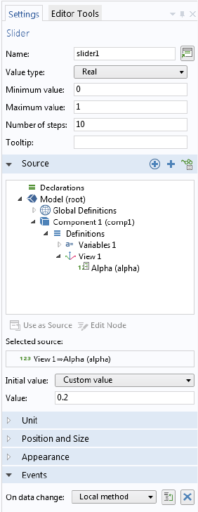
120 |

You can use Data Access in combination with Editor Tools to create a slider or an

input field that sets the transparency level (alpha) of a plot group. The figure

below shows a

Settings window of a slider with the transparency level as Source.

In this case you need to create a method for updating the view that is called to

handle an event from the slider or form object. In the example above, the slider

uses a

Local method defined in the Events section. This method contains one line

of code that updates the view:

useView(getView("/form1/graphics1"), "/form1/graphics1");

Note that different transparency levels are not supported when accessing an

application from a browser using COMSOL Server.

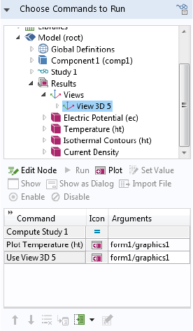
| 121

Note that you can also set a view from the command sequence of, for example, a

button: select a view subnode under the

Views node in the editor tree and click the

Plot button under the tree.

This line of code sets the URL source of the form object webpage1 to the

COMSOL web page:

setWebPageSource("/form1/webpage1", "http://www.comsol.com");

This line of code forms a string containing the screen width and height:

screenSize =

toString(getScreenWidth())+"-by-"+toString(getScreenHeight());

You can present the string with an input field or a data display object using this

string as a source (the string

screenSize needs to be declared first).

122 |

GUI Command Methods

The GUI command methods correspond to the GUI Commands node in the editor

tree. The editor tree is displayed in, for example, the

Choose Commands to Run

section in the

Settings window for a button object in the Application Builder.

EXAMPLE CODE

For examples of how to use fileSaveAs, see the Introduction to Application

Builder.

You can create an application that saves and exits automatically by running the

following lines of code, for example, after solving:

saveModel(model,"C:\\COMSOL\\file.mph");

NAME SYNTAX DESCRIPTION

clearAllMeshes clearAllMeshes()

Clears all meshes.

clearAllSolutions clearAllSolutions()

Clears all solutions.

clearSelection clearSelection(String graphics)

clearSelection(FormObject graphics)

Clears the selection in the given

graphics object.

exit exit()

Exits the application.

fileOpen fileOpen(String name)

Opens a file with the associated

program on the client.

fileSaveAs fileSaveAs(String file)

Downloads a file to the client.

more readable units for

longer times. This format is

localized and the output is

translated to the current

language setting.

For example, you can

retrieve the time in ms by

using

getLastComputationTime("

ms").

NAME SYNTAX DESCRIPTION

| 133

EXAMPLE CODE

The following code overrides the built-in computation time that is available in the

information nodes in the model tree.

long t0 = timeStamp(); // initialize record of computation time

// code and computations

model.setLastComputationTime(timeStamp()-t0); // record computation time

If it is possible to give a rough estimate of the computation time based on the

given inputs of an application, you can update the expected computation time and

display it in an information card stack or a text object. Assume that there is an

integer input called

objects that controls the number of objects in a geometry

array and that the computation roughly increases linearly with this number. The

following code adjusts the expected computation time accordingly.

// Number of minutes of computation time per object

int minutes = objects*2.1;

model.setExpectedComputationTime("About " + minutes + " minutes" );

Sleep

The code below makes the application idle for 1000 ms.

long delay = 1000;

sleep(delay);

This technique can be used to display graphics in a sequence.

For more information on information nodes and information cards, as well as the

sleep method, see the book Introduction to Application Builder.

134 |

Conversion Methods

Conversion methods are used to convert between the different data types

Booleans, integers, doubles, strings, and arrays. These methods are shorthand

versions of conversion methods in the standard Java libraries.

NAME SYNTAX DESCRIPTION

toBoolean boolean toBoolean(String str)

Converts the given string to a

Boolean. (

’true’ returns true, all

other strings return false).

toBoolean boolean [] toBoolean(String[]... strs)

Converts all the strings in the

given array to Booleans (’true’

returns true, all other strings

return false) and returns a

Boolean array.

toBoolean boolean [][] toBoolean(String[][]... strs)

Converts all the strings in the

given matrix to Booleans (

’true’

returns true, all other strings

return false) and returns a

Boolean matrix.

toDouble double toDouble(String str)

Converts the given string to a

double.

toDouble double[] toDouble(String... strs)

Converts all the strings in the

given arrray to doubles and

returns a double array.

toDouble double[][] toDouble(String[]... strs)

Converts all the strings in the

given matrix to doubles and

returns a double matrix.

toDouble double toDouble(float flt)

Converts the given float to a

double.

toDouble double[] toDouble(float... flt)

Converts all the floats in the

given arrray to doubles and

returns a double array.

toDouble double[][] toDouble(float[]... flt)

Converts all the floats in the

given matrix to doubles and

returns a double matrix.

toInt int toInt(String str)

Converts the given string to an

integer.

toInt int[] toInt(String... strs)

Converts all the strings in the

given arrray to integers and

returns an integer array.

| 135

toInt int[][] toInt(String[]... strs)

Converts all the strings in the

given matrix to integers and

returns an integer matrix.

toString String toString(int value)

Converts the given integer to a

string.

toString String toString(double value)

Converts the given double to a

string.

toString String toString(boolean value)

Converts the given Boolean to a

string.

toString String toString(double value, int decimals)

Converts the given double to a

string with the given number of

decimals.

toString String toString(double value, int

decimals,boolean remove)

Converts the given double to a

string with the given number of

decimals with trailing zeros

removed if the Boolean

remove is

true. For example, 10.0000001

with number of decimals set to 3

will return

10 rather than 10.000.

toString String toString(double value, String format)

Converts the given double to a

string using the given format

specifier, which is the same as

java.util.Formatter. See the

corresponding Java format string

documentation for more

information.

toString String[] toString(double[] darray)

Converts all the doubles in the

given array to strings and returns

a string array.

toString String[][] toString(double[][] dmatrix)

Converts all the doubles in the

given matrix to strings and

returns a string matrix.

toString String[] toString(int[] iarray)

Converts all the integers in the

given array to strings and returns

a string array.

toString String[][] toString(int[][] imatrix)

Converts all the integers in the

given matrix to strings and

returns a string matrix.

NAME SYNTAX DESCRIPTION

136 |

Array Methods

Array methods are used to add, remove, insert, and extract subsets of 1D and 2D

arrays.

toString String[] toString(boolean[] barray)

Converts all the Booleans in the

given array to strings and returns

a string array.

toString String[][] toString(boolean[][] bmatrix)

Converts all the Booleans in the

given matrix to strings and

returns a string matrix.

NAME SYNTAX DESCRIPTION

getColumn String[] getColumn(String[][] matrix, int

column)

Returns a String[] for a

specified column in the matrix.

Useful when values have been

read from a file and only certain

columns should be shown in a

table.

getColumn double[] getColumn(double[][] matrix, int

column)

Returns a double[] for a

specified column in the matrix.

getColumn int[] getColumn(int[][] matrix, int column)

Returns an int[] for a specified

column in the matrix.

getColumn boolean[] getColumn(boolean[][] matrix, int

column)

Returns a boolean[] for a

specified column in the matrix.

getSubMatrix String[][] getSubMatrix(String[][] matrix,

int startCol, int endCol, int startRow, int

endRow)

Returns a rectangular submatrix

of the input matrix spanning

columns from startCol to

endCol, and rows from startRow

to endRow.

getSubMatrix double[][] getSubMatrix(double[][] matrix,

int startCol,int endCol, int startRow, int

endRow)

Returns a rectangular submatrix

of the input matrix spanning

columns from startCol to

endCol, and rows from startRow

to endRow.

NAME SYNTAX DESCRIPTION

| 137

getSubMatrix int[][] getSubMatrix(int[][] matrix, int

startCol, int endCol, int startRow, int

endRow)

Returns a rectangular submatrix

of the input matrix spanning

columns from startCol to

endCol, and rows from startRow

to endRow.

getSubMatrix boolean[][] getSubMatrix(boolean[][] matrix,

int startCol, int endCol, int startRow, int

endRow)

Returns a rectangular submatrix

of the input matrix spanning

columns from startCol to

endCol, and rows from startRow

to endRow.

insert String[] insert(String[] array, String value,

int index)

Inserts an element at position

index in an array and returns the

expanded array.

insert double[] insert(double[] array, double value,

int index)

Inserts an element at position

index in an array and returns the

expanded array.

insert int[] insert(int[] array, int value, int

index)

Inserts an element at position

index in an array and returns the

expanded array.

insert boolean[] insert(boolean[] array, boolean

value, int index)

Inserts an element at position

index in an array and returns the

expanded array.

insert String[] insert(String[] array, String[]

value, int[] index)

Inserts elements in an array at

positions given by the index array

and returns the expanded array.

insert double[] insert(double[] array, double[]

value, int[] index)

Inserts elements in an array at

positions given by the index array

and returns the expanded array.

insert int[] insert(int[] array, int[] value, int[]

index)

Inserts elements in an array at

positions given by the index array

and returns the expanded array.

insert boolean[] insert(boolean[] array, boolean[]

value, int[] index)

Inserts elements in an array at

positions given by the index array

and returns the expanded array.

append String[] append(String[] array, String value)

Adds an element to the end of an

array and returns the expanded

array.

append double[] append(double[] array, double value)

Adds an element to the end of an

array and returns the expanded

array.

NAME SYNTAX DESCRIPTION

138 |

append int[] append(int[] array, int value)

Adds an element to the end of an

array and returns the expanded

array.

append boolean[] append(boolean[] array, boolean

value)

Adds an element to the end of an

array and returns the expanded

array.

append String[] append(String[] array, String[]

value)

Adds elements to the end of an

array and returns the expanded

array.

append double[] append(double[] array, double[]

value)

Adds elements to the end of an

array and returns the expanded

array.

append int[] append(int[] array, int[] value)

Adds elements to the end of an

array and returns the expanded

array.

append boolean[] append(boolean[] array, boolean[]

value)

Adds elements to the end of an

array and returns the expanded

array.

remove String[] remove(String[] array, int index)

Removes an element from an

array and returns the shortened

array.

remove double[] remove(double[] array, int index)

Removes an element from an

array and returns the shortened

array.

remove int[] remove(int[] array, int index)

Removes an element from an

array and returns the shortened

array.

remove boolean[] remove(boolean[] array, int index)

Removes an element from an

array and returns the shortened

array.

remove String[] remove(String[] array, int[] index)

Removes elements from an array

and returns the shortened array.

remove double[] remove(double[] array, int[] index)

Removes elements from an array

and returns the shortened array.

remove int[] remove(int[] array, int[] index)

Removes elements from an array

and returns the shortened array.

remove boolean[] remove(boolean[] array, int[]

index)

Removes elements from an array

and returns the shortened array.

NAME SYNTAX DESCRIPTION

| 139

insertRow String[][] insertRow(String[][] matrix,

String[] value, int rowIndex)

Inserts a row into a rectangular

2D array and returns the

expanded array.

insertRow double[][] insertRow(double[][] matrix,

double[] value, int rowIndex)

Inserts a row into a rectangular

2D array and returns the

expanded array.

insertRow int[][] insertRow(int[][] matrix, int[]

value, int rowIndex)

Inserts a row into a rectangular

2D array and returns the

expanded array.

insertRow boolean[][] insertRow(boolean[][] matrix,

boolean[] value, int rowIndex)

Inserts a row into a rectangular

2D array and returns the

expanded array.

insertRow String[][] insertRow(String[][] matrix,

String[][] value, int[] rowIndex)

Adds rows to a rectangular 2D

array and returns the expanded

array.

insertRow double[][] insertRow(double[][] matrix,

double[][] value, int[] rowIndex)

Adds rows to a rectangular 2D

array and returns the expanded

array.

insertRow int[][] insertRow(int[][] matrix, int[][]

value, int[] rowIndex)

Adds rows to a rectangular 2D

array and returns the expanded

array.

insertRow boolean[][] insertRow(boolean[][] matrix,

boolean[][] value, int[] rowIndex)

Adds rows to a rectangular 2D

array and returns the expanded

array.

replaceRow String[][] replaceRow(String[][] matrix,

String[] value, int rowIndex)

Replaces a row in a rectangular

2D array and returns the array.

replaceRow double[][] replaceRow(double[][] matrix,

double[] value, int rowIndex)

Replaces a row in a rectangular

2D array and returns the array.

replaceRow int[][] replaceRow(int[][] matrix, int[]

value, int rowIndex)

Replaces a row in a rectangular

2D array and returns the array.

replaceRow boolean[][] replaceRow(boolean[][] matrix,

boolean[] value, int rowIndex)

Replaces a row in a rectangular

2D array and returns the array.

replaceRow String[][] replaceRow(String[][] matrix,

String[][] value, int[] rowIndex)

Replaces rows in a rectangular

2D array and returns the array.

replaceRow double[][] replaceRow(double[][] matrix,

double[][] value, int[] rowIndex)

Replaces rows in a rectangular

2D array and returns the array.

replaceRow int[][] replaceRow(int[][] matrix, int[][]

value, int[] rowIndex)

Replaces rows in a rectangular

2D array and returns the array.

NAME SYNTAX DESCRIPTION

140 |

replaceRow boolean[][] replaceRow(boolean[][] matrix,

boolean[][] value, int[] rowIndex)

Replaces rows in a rectangular

2D array and returns the array.

appendRow String[][] appendRow(String[][] matrix,

String[] value)

Adds a row to the end of a

rectangular 2D array and returns

the expanded array.

appendRow double[][] appendRow(double[][] matrix,

double[] value)

Adds a row to the end of a

rectangular 2D array and returns

the expanded array.

appendRow int[][] appendRow(int[][] matrix, int[]

value)

Adds a row to the end of a

rectangular 2D array and returns

the expanded array.

appendRow boolean[][] appendRow(boolean[][] matrix,

boolean[] value)

Adds a row to the end of a

rectangular 2D array and returns

the expanded array.

appendRow String[][] appendRow(String[][] matrix,

String[][] value)

Adds rows to the end of a

rectangular 2D array and returns

the expanded array.

appendRow double[][] appendRow(double[][] matrix,

double[][] value)

Adds rows to the end of a

rectangular 2D array and returns

the expanded array.

appendRow int[][] appendRow(int[][] matrix, int[][]

value)

Adds rows to the end of a

rectangular 2D array and returns

the expanded array.

appendRow boolean[][] appendRow(boolean[][] matrix,

boolean[][] value)

Adds rows to the end of a

rectangular 2D array and returns

the expanded array.

removeRow String[][] removeRow(String[][] matrix, int

rowIndex)

Removes a row from a 2D array

and returns the smaller array.

removeRow double[][] removeRow(double[][] matrix, int

rowIndex)

Removes a row from a 2D array

and returns the smaller array.

removeRow int[][] removeRow(int[][] matrix, int

rowIndex)

Removes a row from a 2D array

and returns the smaller array.

removeRow boolean[][] removeRow(boolean[][] matrix, int

rowIndex)

Removes a row from a 2D array

and returns the smaller array.

removeRow String[][] removeRow(String[][] matrix, int[]

rowIndex)

Removes rows from a 2D array

and returns the reduced array.

removeRow double[][] removeRow(double[][] matrix, int[]

rowIndex)

Removes rows from a 2D array

and returns the reduced array.

NAME SYNTAX DESCRIPTION

| 141

removeRow int[][] removeRow(int[][] matrix, int[]

rowIndex)

Removes rows from a 2D array

and returns the reduced array.

removeRow boolean[][] removeRow(boolean[][] matrix,

int[] rowIndex)

Removes rows from a 2D array

and returns the reduced array.

insertColumn String[][] insertColumn(String[][] matrix,

String[] value, int columnIndex)

Adds a column into a rectangular

2D array and returns the

expanded array.

insertColumn double[][] insertColumn(double[][] matrix,

double[] value, int columnIndex)

Adds a column into a rectangular

2D array and returns the

expanded array.

insertColumn int[][] insertColumn(int[][] matrix, int[]

value, int columnIndex)

Adds a column into a rectangular

2D array and returns the

expanded array.

insertColumn boolean[][] insertColumn(boolean[][] matrix,

boolean[] value, int columnIndex)

Adds a column into a rectangular

2D array and returns the

expanded array.

insertColumn String[][] insertColumn(String[][] matrix,

String[][] value, int[] columnIndex)

Adds columns to a rectangular

2D array and returns the

expanded array.

insertColumn double[][] insertColumn(double[][] matrix,

double[][] value, int[] columnIndex)

Adds columns to a rectangular

2D array and returns the

expanded array.

insertColumn int[][] insertColumn(int[][] matrix, int[][]

value, int[] columnIndex)

Adds columns to a rectangular

2D array and returns the

expanded array.

insertColumn boolean[][] insertColumn(boolean[][] matrix,

boolean[][] value, int[] columnIndex)

Adds columns to a rectangular

2D array and returns the

expanded array.

replaceColumn String[][] replaceColumn(String[][] matrix,

String[] value, int columnIndex)

Replaces a column in a

rectangular 2D array and returns

the array.

replaceColumn double[][] replaceColumn(double[][] matrix,

double[] value, int columnIndex)

Replaces a column in a

rectangular 2D array and returns

the array.

replaceColumn int[][] replaceColumn(int[][] matrix, int[]

value, int columnIndex)

Replaces a column in a

rectangular 2D array and returns

the array.

NAME SYNTAX DESCRIPTION

142 |

replaceColumn boolean[][] replaceColumn(boolean[][] matrix,

boolean[] value, int columnIndex)

Replaces a column in a

rectangular 2D array and returns

the array.

replaceColumn String[][] replaceColumn(String[][] matrix,

String[][] value, int[] columnIndex)

Replaces columns in a rectangular

2D array and returns the array.

replaceColumn double[][] replaceColumn(double[][] matrix,

double[][] value, int[] columnIndex)

Replaces columns in a rectangular

2D array and returns the array.

replaceColumn int[][] replaceColumn(int[][] matrix, int[][]

value, int[] columnIndex)

Replaces columns in a rectangular

2D array and returns the array.

replaceColumn boolean[][] replaceColumn(boolean[][] matrix,

boolean[][] value, int[] columnIndex)

Replaces columns in a rectangular

2D array and returns the array.

appendColumn String[][] appendColumn(String[][] matrix,

String[] value)

Adds a column at the end of a

rectangular 2D array and returns

the expanded array.

appendColumn double[][] appendColumn(double[][] matrix,

double[] value)

Adds a column at the end of a

rectangular 2D array and returns

the expanded array.

appendColumn int[][] appendColumn(int[][] matrix, int[]

value)

Adds a column at the end of a

rectangular 2D array and returns

the expanded array.

appendColumn boolean[][] appendColumn(boolean[][] matrix,

boolean[] value)

Adds a column at the end of a

rectangular 2D array and returns

the expanded array.

appendColumn String[][] appendColumn(String[][] matrix,

String[][] value)

Adds columns to the end of a

rectangular 2D array and returns

the expanded array.

appendColumn double[][] appendColumn(double[][] matrix,

double[][] value)

Adds columns to the end of a

rectangular 2D array and returns

the expanded array.

appendColumn int[][] appendColumn(int[][] matrix, int[][]

value)

Adds columns to the end of a

rectangular 2D array and returns

the expanded array.

appendColumn boolean[][] appendColumn(boolean[][] matrix,

boolean[][] value)

Adds columns to the end of a

rectangular 2D array and returns

the expanded array.

removeColumn String[][] removeColumn(String[][] matrix,

int columnIndex)

Removes a column from a

rectangular 2D array and returns

the smaller array.

NAME SYNTAX DESCRIPTION

| 143

removeColumn double[][] removeColumn(double[][] matrix,

int columnIndex)

Removes a column from a

rectangular 2D array and returns

the smaller array.

removeColumn int[][] removeColumn(int[][] matrix, int

columnIndex)

Removes a column from a

rectangular 2D array and returns

the smaller array.

removeColumn boolean[][] removeColumn(boolean[][] matrix,

int columnIndex)

Removes a column from a

rectangular 2D array and returns

the smaller array.

removeColumn String[][] removeColumn(String[][] matrix,

int[] columnIndex)

Removes columns from a

rectangular 2D array and returns

the reduced array.

removeColumn double[][] removeColumn(double[][] matrix,

int[] columnIndex)

Removes columns from a

rectangular 2D array and returns

the reduced array.

removeColumn int[][] removeColumn(int[][] matrix, int[]

columnIndex)

Removes columns from a

rectangular 2D array and returns

the reduced array.

removeColumn boolean[][] removeColumn(boolean[][] matrix,

int[] columnIndex)

Removes columns from a

rectangular 2D array and returns

the reduced array.

matrixSize int[] matrixSize(String[][] matrix)

Returns the number of rows and

columns of a matrix as an integer

array of length 2.

matrixSize int[] matrixSize(double[][] matrix)

Returns the number of rows and

columns of a matrix as an integer

array of length 2.

matrixSize int[] matrixSize(int[][] matrix)

Returns the number of rows and

columns of a matrix as an integer

array of length 2.

matrixSize int[] matrixSize(boolean[][] matrix)

Returns the number of rows and

columns of a matrix as an integer

array of length 2.

transpose String[][] transpose(String[][] matrix)

Returns the transpose of a

matrix.

transpose double[][] transpose(double[][] matrix)

Returns the transpose of a

matrix.

NAME SYNTAX DESCRIPTION

144 |

String Methods

String methods are used to process string variables and string arrays.

transpose int[][] transpose(int[][] matrix)

Returns the transpose of a

matrix.

transpose boolean[][] transpose(boolean[][] matrix)

Returns the transpose of a

matrix.

NAME SYNTAX DESCRIPTION

concat String concat(String separator, String ...

strs)

Concatenates the given

varargs-array of strings into a

single string using the given

separator.

concat String[] concat(String colSepar, String

rowSepar, String[]... matr)

Concatenates the given string

matrix (which can be given as a

varargs of rows) into a single

string. Puts

colSepar between

values of columns of a row, and

rowSepar between rows.

contains boolean contains(String[] strs, String str)

Returns true if the given string

array

strs contains the given

string str.

find int[] find(String[] strs, String str)

Returns an array with the indices

to all occurrences of str in strs.

findIn int findIn(String[] strs, String str)

Returns the index to the first

occurrence of

str in strs or -1 if

no match.

findIn int findIn(String str, String toFind)

Returns the first index of str that

is the start of the substring

toFind. If there is no substring

matching toFind in str, -1 is

returned.

length int length(String str)

Returns the length of the string

str.

replace String replace(String str, String orig,

String replacement)

Returns a string where orig has

been replaced by replacement.

NAME SYNTAX DESCRIPTION

| 145

Collection Methods

Collection methods are used to copy, compare, sort, and merge variables and

arrays.

split String[] split(String str)

Returns an array of strings by

splitting the given string at spaces.

split String[] split(String str, String separator)

Returns an array of strings by

splitting the given string at the

given separator.

substring String substring(String str, int start, int

length)

Returns a substring with the given

length starting at the given

position.

unique String[] unique(String[] strs)

Returns an array of strings with

the unique values in the given

array of strings.

NAME SYNTAX DESCRIPTION

copy String[] copy(String... toCopy)

Returns a copy of the given array

of strings, which can also be

specified as a varargs of strings.

copy String[][] copy(String[]... toCopy)

Returns a copy of the given string

matrix, which can also be

specified as a varargs of rows

(string arrays).

copy double[] copy(double... toCopy)

Returns a copy of the given array

of doubles, which can also be

specified as a varargs of doubles.

copy double[][] copy(double[]... toCopy)

Returns a copy of the given

double matrix, which can also be

specified as a varargs of rows

(double arrays).

copy int[] copy(int... toCopy)

Returns a copy of the given array

of integers, which can also be

specified as a varargs of integers.

copy int[][] copy(int[]... toCopy)

Returns a copy of the given

integer matrix, which can also be

specified as a varargs of rows

(integer arrays).

NAME SYNTAX DESCRIPTION

146 |

copy boolean[] copy(boolean... toCopy)

Returns a copy of the given array

of booleans, which can also be

specified as a varargs of booleans.

copy boolean[][] copy(boolean[]... toCopy)

Returns a copy of the given

boolean matrix, which can also

be specified as a vararags of rows

(boolean arrays).

equals boolean equals(String[] str1, String[] str2)

Returns true if all strings in the

given array are equal and they

have the same number of

elements.

equals boolean equals(String[][] matr1, String[][]

matr2)

Returns true if all strings in the

given matrix are equal and they

have the same number of

elements.

equals boolean equals(int[] ints1, int[] ints2)

Returns true if all integers in the

given array are equal and they

have the same number of

elements.

equals boolean equals(int[][] ints1, int[][] ints2)

Returns true if all integers in the

given matrix are equal and they

have the same number of

elements.

equals boolean equals(double dl1, double dl2, double

relErrorTolerance)

Compares whether the relative

error of two doubles is within

allowed tolerance using abs( ( a -

b ) / b ), where b is the larger of

the doubles (by absolute value).

equals boolean equals(double dl1, double dl2)

Same as above, but uses a default

relErrorTolerance of 0.0001.

equals boolean equals(double[] dbls1, double[]

dbls2, double relErrorTolerance)

Compares the relative errors ( ~

abs( ( a - b) / b ) of elements in

the arrays pairwise and returns

true if all relative errors are

below

relErrorTolerance and

the arrays have the same number

of elements.

equals boolean equals(double[] dbls1, double[]

dbls2)

Same as above, but uses a default

relErrorTolerance of 0.0001.

NAME SYNTAX DESCRIPTION

| 147

equals boolean equals(double[][] dbls1, double[][]

dbls2, double relErrorTolerance)

Compares the relative errors ( ~

abs( ( a - b ) / b ) of elements in

the matrices pairwise and returns

true if all relative errors are

below

relErrorTolerance and

the matrices have the same

number of elements.

equals boolean equals(double[][] dbls1, double[][]

dbls2)

Same as above, but uses a default

relErrorTolerance of 0.0001.

sort sort(String[] strs)

Sorts the given array of strings.

NOTE: The array is sorted in

place.

sort sort(int[] ints)

Sorts the given array of integers.

NOTE: The array is sorted in

place.

sort sort(double[] doubles)

Sorts the given array of doubles.

NOTE: The array is sorted in

place.

sort sort(String[][] strs)

Sorts the given 2D array of

strings. The columns are sorted

by their row values from top to

bottom. NOTE: The array is

sorted in place.

sort sort(int[][] ints)

Sorts the given 2D array of

integers. The columns are sorted

by their row values from top to

bottom. NOTE: The array is

sorted in place.

sort sort(double[][] doubles)

Sorts the given 2D array of

doubles. The columns are sorted

by their row values from top to

bottom. NOTE: The array is

sorted in place.

merge merge(String[]... toMerge)

Returns an array of strings with all

strings merged from the given

arrays.

NAME SYNTAX DESCRIPTION

148 |

Model Builder Methods for Use in Add-ins

For writing add-in method code that operates on the current component, current

mesh, current physics etc. use the methods in the table below.

These methods return the corresponding entity such that the method code in an

add-in can operate on it. When called from an application a method in this

merge merge(int[]... toMerge)

Returns an array of integers with

all integers merged from the two

given arrays.

merge merge(double[]... toMerge)

Returns an array of doubles with

all doubles merged from the two

given arrays.

NAME SYNTAX DESCRIPTION

getCurrentComponent getCurrentComponent()

Returns an object of the type

ModelNode for the current

component.

getCurrentMesh getCurrentMesh()

Returns an object of the type

MeshSequence for the current

mesh.

getCurrentNode getCurrentNode()

Returns an object of the type

ModelEntity for the current

component.

getCurrentPhysics getCurrentPhysics()

Returns an object of the type

Physics for the current physics

interface.

getCurrentPlotGroup getCurrentPlotGroup()

Returns an object of the type

ResultFeature for the current

component.

getCurrentStudy getCurrentStudy()

Returns an object of the type

Study for the current

component.

selectNode selectNode(ModelEntity entity)

Selects a model tree node and

displays its Settings window after

the execution of a method from

the Model Builder.

NAME SYNTAX DESCRIPTION

| 149

category returns null. Also, null is returned if no entity of the corresponding

type exists such that nothing is current.

To learn more about using these methods you can review the Application Builder

settings for one of the built-in add-ins by opening the corresponding MPH file.

In a typical Windows

installation the built-in add-in library is located at

C:\Program Files\COMSOL\COMSOL55\Multiphysics\addins

150 |

Programming Examples

This section contains examples that illustrate solving practical tasks by accessing

and manipulating the model object and using the built-in methods. Note that

additional examples of user-defined methods are provided in the example

applications of the Application Libraries accessible from the

File menu.

Running the Examples

To run the code in the examples below, you can create a method for use in a model

or application. You can, for example, choose the option

Blank Model in the Model

Wizard. To create a new method, go to the

Developer tab in the Model Builder

and click the

New Method button in the ribbon. In the Application Builder, paste

the code into the new method. Finally, you can run the code from the

Developer

tab in the Model Builder by choosing the method you just created from the

Run

Method

toolbar menu.

Visualization Without Solution Data: Grid Data Sets

The section “Results” on page 48 shows how to write code for various parts of the

Results node in the model tree, including

Data Sets, Tables, and Plot Groups. These

examples assume that you have solution data available from solving, for example,

a heat transfer, CFD, or structural mechanics problem.

You can also create visualizations without having associated solution data by either

using grid data sets or using low-level functionality only available through

methods. You can, for example, write code for plotting points and triangles

without any associated solution data. These techniques are useful when creating

applications where customized plot functionality is needed. This section shows

how to use grid data sets, and the next section shows how to use low-level

functionality.

PLOTTING A UNIT SPHERE USING A GRID DATA SET

Grid data sets are available in the Model Builder and can be used in applications

for the sole purpose of visualization without any associated solution data. The

code below creates a visualization of a unit sphere as an isosurface with the

z-coordinate as color data.

| 151

model.func().create("an1", "Analytic");

model.result().dataset().create(

"grid1", "Grid3D");

with(model.result().dataset(

"grid1"));

set(

"source", "data");

set(

"parmin1", -1);

set(

"parmax1", +1);

set(

"parmin2", -1);

set(

"parmax2", +1);

set(

"parmin3", -1);

set(

"parmax3", +1);

set(

"source", "function");

set(

"function", "an1");

endwith();

model.result().create(

"pg1", "PlotGroup3D");

model.result(

"pg1").create("iso1", "Isosurface");

with(model.result(

"pg1").feature("iso1"));

set(

"expr", "x^2+y^2+z^2-1");

set(

"levelmethod", "levels");

set(

"levels", 0.0);

endwith();

model.result(

"pg1").feature("iso1").create("col1", "Color");

with(model.result(

"pg1").feature("iso1").feature("col1"));

set(

"expr", "z");

endwith();

model.result(

"pg1").run();

Comments

If there is no solution-based Data set available, then the Grid3D data set needs to

have a

Function as its Source. In the example above, a default Analytic function is

created with tag

an1. A default Analytic function corresponds to f(x) = x, and its

only purpose is to give the grid data set an evaluation context.

Note: The alternative is to solve a physics problem on a mesh and reference the

corresponding solution data set. The method of referencing a

Function makes it

possible to create visualizations without solution data.

The source for the

Grid3D data set with tag grid1 is set to function, and finally,

the

function property of grid1 is set to an1.

The

Grid3D data set has options for max and min parameter bounds, shown in the

example code above. An additional grid resolution option is not shown in this

example. However, you can learn about its syntax by using

Record Code from the

Model Builder.

152 |

Visualization of Points, Curves, and Surfaces

The following examples describe low-level functionality for visualization that is

only available from methods and is not associated with any solution data. For

visualization based on solution data, see the section “Results” on page 48.

The examples below illustrate using the following plot types:

• Point Data

• Line Data

• Surface Data

• Tube Data

• Arrow Data

• Annotation Data

Once created, the plot type names are visible in the Settings window of each plot.

In addition to the properties modified by the examples below, in the

Settings

window of these plot types, you can see the number of geometric entities created,

such as number of points, line segments, and triangles. Just as for other types of

plots, you can also change the

Range of color and data, as well as Coloring and Style.

POINTS IN 2D

The following code plots a circle of points using the Point Data plot type.

// A circle of points

String pgTag = model.result().uniquetag(

"pg");

ResultFeature pg = model.result().create(pgTag, 2);

ResultFeature plot = pg.create(

"pt1", "PointData");

int N = 17;

double[][] p = new double[2][N];

double[] color = new double[N];

double R = 1000;

for (int i = 0; i < N; i++) {

double angle = i*2*Math.PI/N;

p[0][i] = R*Math.cos(angle);

p[1][i] = R*Math.sin(angle);

color[i] = p[1][i];

}

plot.set(

"pointdata", p)

.set(

"colordata", color)

.set(

"coloring", "colortable");

plot.run();

Comments

The first line

String pgTag = model.result().uniquetag("pg");

| 153

creates a unique tag for the plot group to be created. This is useful if you intend

to add a varying number of plot groups in your model or application.

The line

ResultFeature pg = model.result().create(pgTag, 2);

creates a 2D Plot Group using the newly created unique tag. The second argument

create defines the dimension of the plot group (2 for 2D, 3 for 3D, etc.).

The line

ResultFeature plot = pg.create("pt1", "PointData");

creates a plot of the type PointData. This plot type is only available through

methods.

The middle part of the example code generates the points making up the circle.

The point coordinates are stored in the

2-by-N array p, along with color data in the

array

color of length N. The color data is, in this example, simply based on the

index of the points and is used to control the coloring of each point based on a

color table.

The last few lines populate the fields of the

Point Data plot.

plot.set("pointdata", p)

.set(

"colordata", color)

.set(

"coloring", "colortable");

The property pointdata takes the 2-by-N array p as its input. The options for the

coloring property are colortable or uniform.

To learn about the syntax for the additional properties available for a

Point Data

plot, you can run the above code in a blank model, browse to the

Settings window

for the

Point Data plot, click Record Code, and change the corresponding plot

properties. Note that the name of the plot type in the

Settings window of the plot

in the model tree is

Point Data.

TURNING OFF MODEL HISTORY

When using this type of low-level functionality for larger sets of data, such as a

large number of points, the stored model history may become excessively large.

Because of this, it is recommended to temporarily turn off model history recording

when using this type of functionality; see “Turning Off and Reset The Model

History” on page 52.

POINTS IN 3D

The following code plots points in an undulating pattern in 3D using the Point

Data

plot type.

// Undulating points in 3D

154 |

String pgTag = model.result().uniquetag("pg");

ResultFeature pg = model.result().create(pgTag, 3);

ResultFeature plot = pg.create(

"pt1", "PointData");

int N = 37;

double[][] p = new double[3][N];

double[] color = new double[N];

double R = 1000;

for (int i = 0; i < N; i++) {

double angle = i*2*Math.PI/N;

p[0][i] = R*Math.cos(angle);

p[1][i] = R*Math.sin(angle);

p[2][i] = R*Math.cos(3*angle);

color[i] = p[1][i];

}

plot.set(

"pointdata", p)

.set(

"colordata", color)

.set(

"coloring", "colortable")

.set(

"sphereradiusscale", 1);

plot.run();

selectNode(pg);

Comments

When plotting 3D points the line

model.result().create(pgTag, 3);

has the second argument set to 3 in order to create a 3D Plot Group. In 3D, the

point coordinates,

p is a 3-by-N array.

The line

.set("sphereradiusscale", 1);

controls the radius of the sphere used to render each point.

To automatically display the newly created plot, the line

selectNode(pg);

is added last in the code segment.

To get a denser set of points, you can increase the integer

N to, say, 370.

CURVE IN 3D

The following code plots line segments in the shape of a 3D helix using the Line

Data

plot type.

// A 3D helix from line segments

String pgTag = model.result().uniquetag(

"pg");

ResultFeature pg = model.result().create(pgTag, 3);

ResultFeature plot = pg.create(

"line1", "LineData");

int N = 100;

double[][] p = new double[3][N];

int[][] t = new int[2][N-1];

for (int i = 0; i < N; i++) {

double s = 4*Math.PI*i/N;

| 155

p[0][i] = s/5;

p[1][i] = Math.sin(s);

p[2][i] = Math.cos(s);

if (i > 0) {

t[0][i-1] = i-1;

t[1][i-1] = i;

}

plot.set(

"pointdata", p)

.set(

"elementdata", t);

plot.run();

selectNode(pg);

Comments

The line

ResultFeature plot = pg.create("line1", "LineData");

creates a plot of the type LineData. This plot type is only available through

methods. Just as for

Point Data plots, the point coordinates p is a 3-by-N array. In

addition to

pointdata, the LineData plot type takes elementdata as its input. In

the example, this is represented by the

2-by-N array t and contains indexes to the

columns of

p, corresponding to the start and end points of the lines.

In a similar way, line segments can be plotted in 2D by creating a 2D plot group

and by letting the point coordinates be a

2-by-N array. See also “Points in 2D” on

page 152.

TRIANGULATED SHAPE IN 2D

The following code plots triangles in the shape of a 2D pentagon by using the

Surface Data plot type.

// A 2D pentagon from triangles

String pgTag = model.result().uniquetag(

"pg");

ResultFeature pg = model.result().create(pgTag, 2);

ResultFeature plot = pg.create(

"surf1", "SurfaceData");

int N = 5;

double[][] p = new double[2][N+1];

int[][] t = new int[3][N];

p[0][0] = 0;

p[1][0] = 0;

for (int i = 0; i < N; i++) {

double angle = i*2*Math.PI/N;

p[0][i+1] = Math.cos(angle);

p[1][i+1] = Math.sin(angle);

t[0][i] = 0;

t[1][i] = i+1;

t[2][i] = 1+(i+1)%N;

}

plot.set(

"pointdata", p)

.set(

"elementdata", t);

plot.run();

156 |

selectNode(pg);

Comments

The line

ResultFeature plot = pg.create("surf1", "SurfaceData");

creates a plot of the type SurfaceData. This plot type is only available through

methods. Just as for 2D

Point Data plots, the point coordinates p is a 2-by-N array.

In addition to

pointdata, and similar to the LineData plot type, the SurfData

plot type takes

elementdata as its input. In the example, this is represented by the

3-by-N array t and contains indexes to the columns of p, corresponding to the

vertexes of the triangles. The ordering of the point indexes in the array

t is not

important for 2D Surface Data plots.

FUNCTION SURFACE IN 3D

The following code plots triangles in the shape of a 3D rotationally symmetric

sinc-function surface by using the

Surface Data plot type.

// A 3D sinc(r) function surface

String pgTag = model.result().uniquetag(

"pg");

ResultFeature pg = model.result().create(pgTag, 3);

ResultFeature plot = pg.create(

"surf1", "SurfaceData");

int Nx = 51;

int Ny = 51;

double[][] p = new double[3][Nx*Ny];

int[][] t = new int[3][2*(Nx-1)*(Ny-1)];

double[] color = new double[Nx*Ny];

int pos = 0;

for (int i = 0; i < Ny; i++) {

for (int j = 0; j < Nx; j++) {

double x = 20*(j-Nx/2)/Nx;

double y = 20*(i-Ny/2)/Ny;

double r = Math.sqrt(x*x+y*y);

double z = 4*((r == 0) ? 1 : (Math.sin(r)/r));

p[0][pos] = x;

p[1][pos] = y;

p[2][pos] = z;

color[pos] = z;

pos++;

}

pos = 0;

for (int i = 0; i < Ny-1; i++) {

for (int j = 0; j < Nx-1; j++) {

int p00 = Nx*i+j;

int p01 = Nx*i+j+1;

int p10 = Nx*(i+1)+j;

int p11 = Nx*(i+1)+j+1;

t[0][pos] = p00;

t[1][pos] = p01;

t[2][pos] = p11;

| 157

pos++;

t[0][pos] = p00;

t[1][pos] = p11;

t[2][pos] = p10;

pos++;

}

plot.set(

"pointdata", p)

.set(

"elementdata", t)

.set(

"colordata", color)

.set(

"coloring", "colortable");

plot.run();

selectNode(pg);

Comments

This example is similar to “Triangulated Shape in 2D” on page 155, but with the

point array being a

3-by-N array for 3D surfaces. For Surface Data plots in 3D, the

ordering of the indexes in the

elementdata array t matters. It determines the

direction of the surface normal, which is used for the lighting effect when using

Scene Light in the Graphics window. The surface normal of a triangle is determined

according to the “right-hand rule”. In mathematical terms, the surface normal is

defined as the vector product:

where the indexes into

t represent the rows in one of the columns of t and p

represents a column in the array of points

To ensure that the lighting effect produces expected results, the triangle surface

normal directions need to consistently point in the same direction as the intended

overall surface normal direction. As an alternative to making sure that the indexes

come in the correct order, the normal direction may be given as an additional

input to a

Surface Data plot. This is shown in the next example section, Sphere in

3D.

SPHERE IN 3D

The following code plots triangles in the shape of a 3D sphere by using the Surface

Data

plot type.

// A coarse sphere with user-supplied normals

int Nx = 20;

int Ny = 10;

String pgTag = model.result().uniquetag(

"pg");

ResultFeature pg = model.result().create(pgTag, 3);

ResultFeature plot = pg.create(

"surf1", "SurfaceData");

double[][] p = new double[3][Nx*Ny];

double[][] normals = new double[3][Nx*Ny];

int[][] t = new int[3][2*(Nx-1)*(Ny-1)];

double[] color = new double[Nx*Ny];

npt 1[][]p t 0[][]–()p t 2[][]p t 0[][]–()×=

158 |

int pos = 0;

double R = 10;

for (int i = 0; i < Ny; i++) {

for (int j = 0; j < Nx; j++) {

double theta = Math.PI*i/(Ny-1);

double phi = 2*Math.PI*j/(Nx-1);

double x = R*Math.sin(theta)*Math.cos(phi);

double y = R*Math.sin(theta)*Math.sin(phi);

double z = R*Math.cos(theta);

p[0][pos] = x;

p[1][pos] = y;

p[2][pos] = z;

normals[0][pos] = x;

normals[1][pos] = y;

normals[2][pos] = z;

color[pos] = z;

pos++;

}

pos = 0;

for (int i = 0; i < Ny-1; i++) {

for (int j = 0; j < Nx-1; j++) {

int p00 = Nx*i+j;

int p01 = Nx*i+j+1;

int p10 = Nx*(i+1)+j;

int p11 = Nx*(i+1)+j+1;

t[0][pos] = p00;

t[1][pos] = p01;

t[2][pos] = p11;

pos++;

t[0][pos] = p00;

t[1][pos] = p11;

t[2][pos] = p10;

pos++;

}

plot.set(

"pointdata", p)

.set(

"elementdata", t)

.set(

"colordata", color)

.set(

"normaldata", normals)

.set(

"coloring", "colortable");

plot.run();

selectNode(pg);

Comments

In this example, information about the surface normal direction is not given

implicitly by the triangle orientation, but instead explicitly by the parameter

normaldata by means of the 3-by-Nx*Ny array normals containing surface normal

vectors at each point. The normal vectors do not need to be normalized; only the

direction is used. The coloring of the sphere is based on the z-coordinate of each

triangle point and is stored for each point in the

3-by-Nx*Ny array color.

| 159

The sphere is constructed from a discrete grid defined in terms of spherical

coordinate angles, where each grid cell is divided into two triangles. The number

of triangles

t is then given by 2*(Nx-1)*(Ny-1).

TUBE PLOT IN 3D, LOGARITHMIC SPIRAL

The following code plots a tube in 3D in the shape of a logarithmic spiral by using

the

Tube Data plot type.

// A logarithmic tube spiral in 3D

String pgTag = model.result().uniquetag(

"pg");

ResultFeature pg = model.result().create(pgTag, 3);

ResultFeature plot = pg.create(

"tube1", "TubeData");

int N = 1000;

double[][] p = new double[3][N];

double[] radius = new double[N];

double[] color = new double[N];

for (int i = 0; i < N; i++) {

double par = 0.005*i;

p[0][i] = Math.exp(par)*Math.cos(10*par);

p[1][i] = Math.exp(par)*Math.sin(10*par);

p[2][i] = 0.1*i;

radius[i] = 0.2*Math.sqrt(i+1);

color[i] = i;

}

plot.set(

"pointdata", p)

.set(

"radiusdata", radius)

.set(

"colordata", color)

.set(

"coloring", "colortable");

plot.run();

selectNode(pg);

Comments

A Tube Data plot is similar to a Point Data, plot but with an absolute radius array

given as an argument to

radiusdata. For the Point Data plot type, there is a similar

sphereradiusscale.

ARROWS IN 2D

The following code plots arrows in a circular pattern by using the Arrow Data plot

type.

// Arrows in a circular pattern in 2D

String pgTag = model.result().uniquetag(

"pg");

ResultFeature pg = model.result().create(pgTag, 2);

ResultFeature plot = pg.create(

"arrow1", "ArrowData");

int N = 17;

double[][] p = new double[2][N];

double[][] vec = new double[2][N];

double len = 0.2;

for (int i = 0; i < N; i++) {

160 |

double angle = 2*Math.PI*i/N;

p[0][i] = Math.cos(angle);

p[1][i] = Math.sin(angle);

vec[0][i] = -len*p[0][i];

vec[1][i] = -len*p[1][i];

}

plot.set(

"pointdata", p)

.set(

"vectordata", vec);

plot.run();

selectNode(pg);

Comments

An Arrow Data plot associates an array of vectors, in the example vec, to each point

ARROWS IN 3D

The following code plots arrows in a logarithmic spiral pattern by using the Arrow

Data

plot type.

// Arrows in a logarithmic spiral pattern in 3D

String pgTag = model.result().uniquetag(

"pg");

ResultFeature pg = model.result().create(pgTag, 3);

ResultFeature plot = pg.create(

"arrow1", "ArrowData");

int N = 1000;

double[][] p = new double[3][N];

double[][] vec = new double[3][N];

double[] color = new double[N];

for (int i = 0; i < N; i++) {

double par = 0.005*i;

p[0][i] = Math.exp(par)*Math.cos(10*par);

p[1][i] = Math.exp(par)*Math.sin(10*par);

p[2][i] = 0.1*i;

double len = Math.sqrt(p[0][i]*p[0][i]+p[1][i]*p[1][i]+p[2][i]*p[2][i]);

for (int j = 0; j < 3; j++) {

vec[j][i] = 4*p[j][i]/len;

}

color[i] = i;

}

plot.set(

"pointdata", p)

.set(

"vectordata", vec)

.set(

"colordata", color)

.set(

"coloring", "colortable");

plot.run();

selectNode(pg);

Comments

In this example, in addition to the example in the section “Arrows in 2D”, color

data is used based on the point index.

| 161

ANNOTATIONS IN 2D

The following code renders text strings in a circular pattern by using the

Annotation Data plot type.

// Letters in a circlular pattern in 2D

String pgTag = model.result().uniquetag(

"pg");

ResultFeature pg = model.result().create(pgTag, 2);

for (int i = 0; i < 26; i++) {

double angle = 2*Math.PI*i/26;

ResultFeature plot = pg.create(

"ann"+i, "AnnotationData");

plot.set(

"pos", new double[]{Math.cos(angle), Math.sin(angle)})

.set(

"text", "ABCDEFGHIJKLMNOPQRSTUVWXYZ".substring(i, i+1))

.set(

"showpoint", false);

}

pg.run();

selectNode(pg);

Comments

The property pos takes as its input an array of length 2 representing 2D

coordinates for the position of the string to be rendered. The property

text takes

as its input the string to be rendered. The Boolean property

showpoint determines

if a point, at the 2D coordinate position, should be rendered or not.

ANNOTATIONS IN 3D WITH LATEX SYNTAX

The following code renders text strings with Greek letters of different colors at the

corners of a cube by using the

Annotation Data plot type.

// Greek letters at the corners of a cube

String pgTag = model.result().uniquetag(

"pg");

ResultFeature pg = model.result().create(pgTag, 3);

String[] texts = {

"\\alpha", "\\beta", "\\gamma", "\\delta", "\\epsilon",

"\\zeta", "\\eta", "\\theta"};

String[] colors = {

"black", "blue", "cyan", "gray", "green", "magenta", "red",

"yellow"};

for (int x = 0; x < 2; x++) {

for (int y = 0; y < 2; y++) {

for (int z = 0; z < 2; z++) {

int index = x+2*y+4*z;

ResultFeature plot = pg.create(

"ann"+index, "AnnotationData");

plot.set(

"pos", new double[]{x, y, z})

.set(

"text", "$"+texts[index]+"$")

.set(

"latexmarkup", true)

.set(

"color", colors[index]);

}

pg.run();

selectNode(pg);

162 |

Comments

The Boolean property latexmarkup determines if the text should be interpreted

using LaTeX syntax or not.

Reading and Writing Data to File

The Application Builder provides several built-in methods for reading and writing

different types of files: text files, CSV-files, Excel

files (requires LiveLink™ for

Excel

), and binary files. These file methods are listed in the table “File Methods”

on page 96.

Note that easy-to-use user-interface-based techniques for reading and writing to

file are available in the Form editor of the Application Builder. It is recommended

that you consider those techniques first before using the programming-based ways

described in this section. For more information, see the book Introduction to

Application Builder and “GUI Command Methods” on page 122. There, you

can also find information on the various file schemes used in the Application

Builder for reading and writing files when running applications in a web browser.

READING AND WRITING TEXT AND SPREADSHEET FILES OVERVIEW

The following built-in methods are available for reading and writing text files:

• readFile

• readMatrixFromFile

• readStringMatrixFromFile

• readCSVFile

• writeFile

• writeCSVFile

In addition, you can use the low-level methods available in the class CsReader to

read text files line by line or character by character. See the next section,

“Processing Text Files using the CsReader and CsWriter Classes” on page 177, for

more information.

If you have a LiveLink™ for

Excel

license, then the following methods are

available for reading and writing Microsoft Excel Workbook files:

• readExcelFile

• writeExcelFile

| 163

INTRODUCTION TO READING FILES WITH A CSV-FILE EXAMPLE

Assume that you want to automate a certain thermal analysis of a circuit board by

creating an application that reads in data from a spreadsheet. Further assume that

information about the circuit board components is given by a proprietary format

in a spreadsheet with columns for component type, heat dissipation, locations, and

sizes. Assume that such a file looks like:

B,0,0,0,-1.57,350,200,1.57

B,3,30,10,0,40,10,2

C,1,100,30,0,3,10,

C,1,110,30,0,3,10,

B,4,30,30,0,40,10,2

...

C,1,200,30,0,3,10,

B,10,100,150,0,10,20,30

B,10,130,150,0,10,20,30

B,10,160,150,0,10,20,30

Each row of the spreadsheet represents a different component. The first column

can contain a letter, either B or C, denoting that the component can be modeled

as either a

Block or a Cylinder primitive. The next column is the total heat

dissipation within the component (measured in watts). The next three columns

represent the location of the component in the global Cartesian coordinate system

(measured in millimeters). Lastly, if the row contains a block component, there are

three more columns that denote the width, depth, and height of the block. If the

row contains a cylinder component, then there are two more columns that contain

the radius and height information, respectively.

For the example shown above, the first row of the spreadsheet represents the

circuit board itself, which is 1.57 mm thick and 350 mm x 200 mm. It is offset

from the origin by -1.57 mm in the z-direction and does not dissipate any heat.

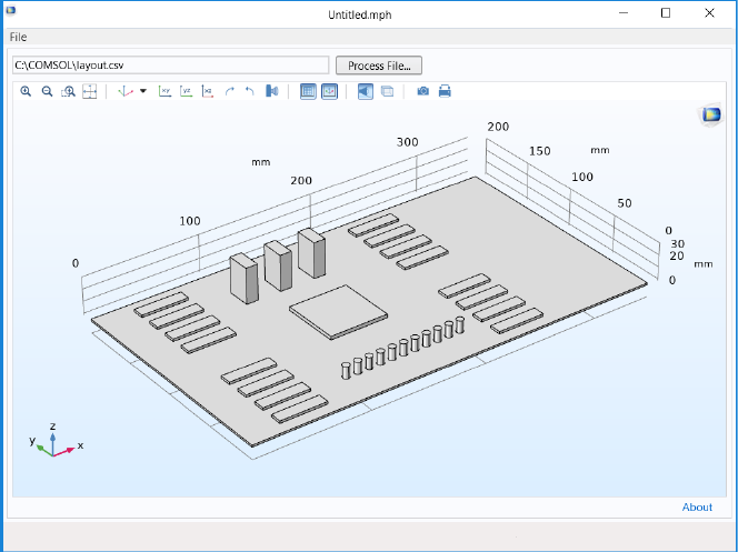
164 |

You can write the data in the spreadsheet out to a comma-delimited text file, also

known as a CSV-file. The user interface of the application used to read the data is

shown in the figure below.

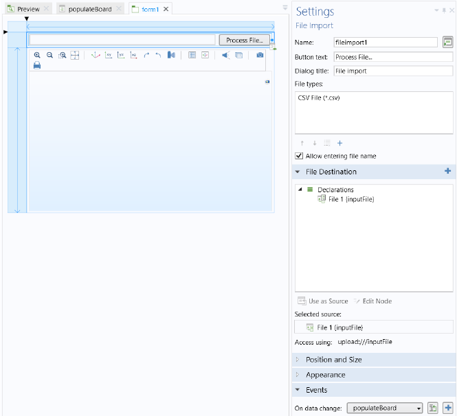
| 165

The Settings window for the File Import form object is shown in the figure below.

In the

Settings window, CSV File (*.csv) is added to the File types list. When

browsing for the file, this setting will filter out any file that is not a CSV-file.

There is also a

File Declaration called File 1, which is referenced by the file scheme

syntax

upload:///inputFile in the method populateBoard, which is used to

read and process the data. The method is called as an event shown at the bottom

of the

Settings window of the File Import form object in the Events section.

Note that if you would like to open a file browser from a button or a menu item,

instead of using a

File Import object, you can create a method that calls the built-in

method

importFile; for example

importFile("file1");

assuming there is a file declaration file1.

The method

populateBoard is listed below.

String[][] D = readCSVFile("upload:///inputFile");

model.geom("geom1").feature().clear();

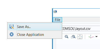
166 |

for (int k = 0; k < D.length; k++) {

if (D[k][0].equals("B")) { // Read in a block

model.geom("geom1").create("P"+k, "Block").set("pos", new

String[]{D[k][2], D[k][3], D[k][4]});

model.geom("geom1").feature("P"+k).set("size", new String[]{D[k][5],

D[k][6], D[k][7]});

}

else if (D[k][0].equals("C")) { // Read in a cylinder

model.geom("geom1").create("P"+k, "Cylinder").set("pos", new

String[]{D[k][2], D[k][3], D[k][4]});

model.geom("geom1").feature("P"+k).set("r", D[k][5]);

model.geom("geom1").feature("P"+k).set("h", D[k][6]);

}

model.geom("geom1").feature("P"+k).set("selresult", "on");

model.variable().remove("var"+k);

model.variable().create("var"+k).model("comp1");

model.variable("var"+k).selection().named("geom1_P"+k+"_dom");

model.variable("var"+k).set("Q", D[k][1]);

}

model.geom("geom1").run();

zoomExtents(

"/form1/graphics1");

Comments

In the first line, the data read from the CSV-file is stored in the 2D array D. The

rest of the code parses this array and populates the various parts of a model object.

The application allows you to save the result as an MPH-file with variables defined

for the heat sources and geometry objects defined for the components, as shown

in the figures below.

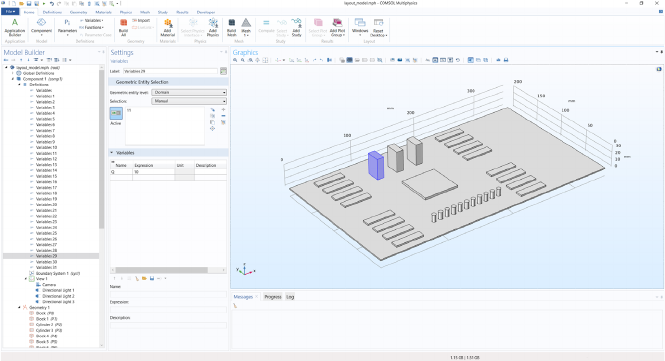
| 167

You can download the MPH-file for this app from:

https://www.comsol.com/model/using-text-files-to-automate-model-preprocessing-46721

READING EXCEL FILES

The application described above can easily be extended to also read Microsoft

Excel

Workbook files. Note that this requires LiveLink™ for Excel

. In the

Settings window for the File Import form object, you can add Microsoft Excel

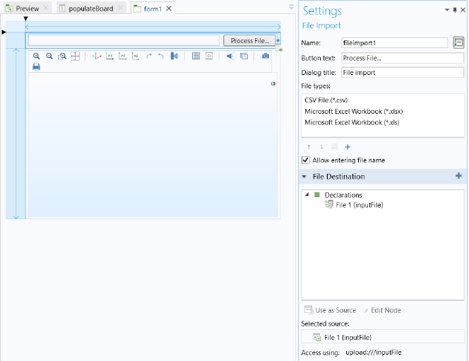
168 |

Workbook (*.xlsx) and Microsoft Excel Workbook (*.xls) to the File types section, as

shown in the figure below.

The next step is to add a few lines of code in the beginning of the method

populateBoard, as shown below.

String file_name = getFilePath("upload:///inputFile");

if (file_name.endsWith(

".xls") || file_name.endsWith(".xlsx"))

D = readExcelFile(

"upload:///inputFile");

else if (file_name.endsWith(

".csv"))

D = readCSVFile(

"upload:///inputFile");

else

error(

"Unknown file type.");

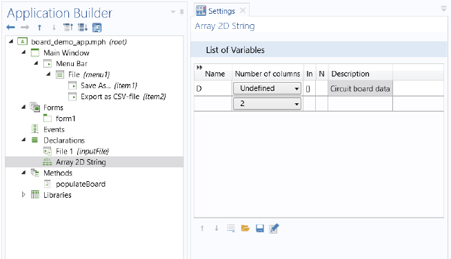
| 169

Comments

Here the 2D array D is defined as a global array in the Declarations node in the

application tree, as shown below.

Alternatively, it can be declared as an array that is local to the method by adding

the line

String[][] D = null;

before the if statement. Which option to choose depends on how you would like

to use the 2D array data after having read the file.

The method

getFilePath returns the full path and name of the uploaded file. The

if statements control which method is used to read the file based on its file

extension. The file extension is retrieved with the Java

method endsWith(),

which belongs to the

String class. Note that you can see which methods are

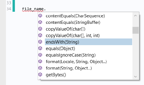
170 |

available for a string by typing the name of the string followed by a period and

Ctrl+Space, as shown in the figure below.

WRITING CSV-FILES

You can write to a CSV-file using four different call syntaxes for the method

writeCSVFile, depending on if the contents are strings or doubles and whether

you would like to overwrite an already existing file or appending to its contents.

In the case above, the contents are a mix of numbers and characters, so the 2D

array storing the information needs to be a string array.

Assume that we would like to move one of the components, say, the second to last

one, in the file listed above. We would like to change the corresponding line in the

file from

B,10,130,150,0,10,20,30

B,10,130,140,0,10,20,30

This corresponds to a change in the y-coordinate of one of the blocks from 150 to

140.

The following code shows how to make this change and then write data on this

format, assuming that the array

D has been declared as a global variable in the

Declarations node, as described above.

int[] sz = matrixSize(D);

D[sz[0]-2][3] =

"140.0";

writeCSVFile(

"temp:///my_layout.csv", D);

fileSaveAs(

"temp:///my_layout.csv");

| 171

Comments

The first line stores the size of the 2D array (or matrix) D in a 1-by-2 array (or

vector)

sz. The second line sets the string value of the y-coordinate of the block

of the second-to-last row in

The line

writeCSVFile("temp:///my_layout.csv", D);

writes the data to a file my_layout.csv in a temporary folder whose location is

determined by the

Preferences of either COMSOL Multiphysics or COMSOL

Server, depending on which software is used to run the application. For example,

in a typical Windows

installation of COMSOL Multiphysics, the location will be

similar to

C:\Users\paul\AppData\Local\Temp\

where the username is paul.

WRITING FILES IN GENERAL

Note that as a first step in the example above, the file is written to a temporary file

using the

writeCSVFile method. This step is done automatically by the

application. In the second step, the method

fileSaveAs opens a file browser and

lets the user of the application choose the file location; for example, a folder on

the computer’s local file system or to a network folder. This extra step is needed

in order for the application to function in a web browser. Due to the security

settings of a typical web browser, the application is not permitted to automatically

save a file to an arbitrary location. Instead, the application is allowed to save to a

few specific locations, including the

temp folder, whose location is specified in the

Preferences settings. The other locations are the user and common folders, also

specified in the

Preferences settings. For more information, see the Introduction

to Application Builder.

WRITING EXCEL FILES

If you have licensed LiveLink™ for Excel

, then you can write to a Microsoft Excel

Workbook file in a way that is similar to that of a CSV-file, with the exception that

the append option is not available. The following code, corresponding to the

previous CSV-file example, shows how to write to an Excel file.

int[] sz = matrixSize(D);

D[sz[0]-2][3] =

"140.0";

writeExcelFile(

"temp:///my_layout.xlsx", D);

fileSaveAs(

"temp:///my_layout.xlsx");

172 |

READING MATRIX FILES

Reading files with numerical data in matrix format is easiest when using the

readMatrixFromFile method. This method assumes that the file has the

spreadsheet format, as available in the model tree

Export node. The example below

shows a file on the spreadsheet format.

% Model: my_model.mph

% Version: COMSOL 5.4.0.123

% Date: May 1 2018, 8:00

% Dimension: 1

% Nodes: 5

% Expressions: 1

% Description: Line graph

% x y

1.2 -0.45

1.11 -0.3

1.0440468877558806 -0.38655264416650392

1.041666666666667 -0.49166666666666667

1.02 -0.15

The first few lines with comments start with the character % and are ignored by the

readMatrixFromFile method. You can optionally omit such lines and just have

the numerical part of a file read by

readMatrixFromFile. Assume that this file is

uploaded to an application using a

File Import form object and a File declaration

file1. The following code can then be used to read the data into a double array p.

double p[][] = readMatrixFromFile("upload:///file1”);

The code below shows how to both import and visualize these points in an

application that, in addition to a

File Import form object and a File declaration

file, has a form form1 and a graphics object graphics1.

double p[][] = readMatrixFromFile("upload:///file1");

double pt[][] = transpose(p);

String pgTag = model.result().uniquetag(

"pg");

ResultFeature pg = model.result().create(pgTag, 2);

ResultFeature plot = pg.create(

"pt1", "PointData");

plot.set(

"pointdata", pt);

plot.run();

useGraphics(model.result(pgTag),

"form1/graphics1");

Reading files on the spreadsheet format as a string array can be done with the

method

readStringMatrixFromFile. Also, in this case, the comment lines will be

ignored. The code below shows how you can replace the first few lines in the

above example using

readStringMatrixFromFile instead of

readMatrixFromFile.

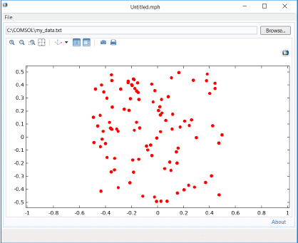
| 173

String p[][] = readStringMatrixFromFile("upload:///file1");

double pt[][] = transpose(toDouble(p));

The method readStringMatrixFromFile is most useful when parts of the read

file contains text.

WRITING MATRIX FILES

To write numerical matrix data to file, you can use the method writeFile.

Assume that you want to write a matrix of random 2D coordinate values to a file

on the spreadsheet format; for example:

-0.3604014719437022 0.06964952539192892

-0.043869911848460674 -0.14152948348300798

0.08279441507358754 0.3101282179426158

...

0.4419748551931647 0.4139106589169702

0.15830016844077643 -0.08445989494858042

0.38236182707603905 0.4837445802317204

The code below shows how to do this.

int N = 100;

double[][] p = new double[N][2];

for (int k = 0; k < N; k++) {

p[k][0] = Math.random()-0.5;

p[k][1] = Math.random()-0.5;

}

writeFile(

"temp:///my_data.txt", p);

fileSaveAs(

"temp:///my_data.txt");

The resulting file can now be read back in and plotted by using the code of the

previous example. The result, in an application, may look like the figure below.

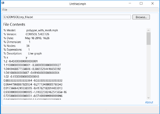
174 |

Note that you can append data to an already existing file by providing an

additional Boolean input argument; for example:

writeFile("temp:///my_data.txt", p,true);

fileSaveAs(

"temp:///my_data.txt");

If you would like to export a matrix with a mix of numeric and text data, you can

use the

writeFile method with a string array instead of a double array. The syntax

for this case is otherwise identical to that of the double array shown in the example

above.

READING A TEXT FILE TO A STRING

For reading text files into a string, you can use the method readFile. A

straightforward use of

readFile is for previewing a text file; for example, before

importing and parsing it, as illustrated by the example application in the figure

below.

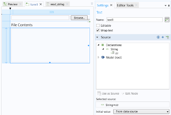
| 175

This application has two form objects: a File Import form object referencing a File

declaration

file1 and a Text form object referencing a string str declared in the

Declarations node as a global variable.

The

File Import form object has an Event that calls the method read_string upon

data change.

This method has one line of code, as shown below.

str = readFile("upload:///file1");

Since the Text object is referencing the global string str, the contents of the file

are displayed in the

Text object immediately after import.

Parsing of smaller text files can be done with

readFile in combination with the

many text processing methods available in the

String class. However, it is often

more efficient to use methods in the

CsReader class, as described in the section

“Processing Text Files using the CsReader and CsWriter Classes” on page 177,

especially for larger text files. The reason is that when using the

readFile method,

the entire file is read into a string with all its contents kept in memory; whereas

when using the

CsReader class methods, only small portions of the file are kept in

memory at any given time.

If you would like to parse smaller text files using

readFile, then the built-in

“String Methods” on page 144 are useful. The example code below illustrates

using the built-in methods

findIn, substring, split, as well as the regular Java

methods

System.getProperty and String.startsWith. The example parses the

header of a text file containing polygon information to retrieve information about

the number of points of each polygon in the main body of the file (not shown) as

176 |

well as the number of properties (for example, color or material property). The

header portion of the file may look like the example below.

Demo file for string parsing

Created on May 1st 2018

begin_header

number_of_points 4

number_of_properties 4

end_header

The code for parsing the header is listed below. It stores the number of points and

properties in the variables

n_of_points and n_of_properties, respectively. To

keep things simple, no error handling is done. For example, the code assumes that

there is exactly one instance of

begin_header and end_header.

int n_of_points = 0;

int n_of_properties = 0;

String fileContents = readFile(

"upload:///file1");

String eol = System.getProperty(

"line.separator"); // find the system end of line

int headerBeginIndex = findIn(fileContents,

"begin_header");

int headerEndIndex = findIn(fileContents,

"end_header");

String headerContents = substring(fileContents, headerBeginIndex,

headerEndIndex-headerBeginIndex); // Convert to string array by splitting at

each line.

String[] headerContentsArr = split(headerContents, eol);

int ix = 1;

String[] headerRowArr = new String[2];

do {

// Split each line at space.

headerRowArr = split(headerContentsArr[ix],

" ");

if (headerRowArr.length == 2) {

if (headerRowArr[0].trim().equalsIgnoreCase(

"number_of_points"))

n_of_points = toInt(headerRowArr[1]);

if (headerRowArr[0].trim().equalsIgnoreCase(

"number_of_properties"))

n_of_properties = toInt(headerRowArr[1]);

}

ix++;

} while (ix < headerContentsArr.length);

The Java

String class has many methods for text processing. See the online Java

documentation for more information.

WRITING A STRING TO A TEXT FILE

The following example shows how to use the method writeFile to write a string

to file.

String contents = "# Created by me\r\n"

+"# Version 1.0 of this file format \r\n"

+"# Body follows\r\n"

+"0 1 \r\n"

| 177

+"2 3\r\n"

+"4 5\r\n";

writeFile(

"temp:///my_data.txt", contents);

fileSaveAs(

"temp:///my_data.txt");

The use of the file scheme syntax temp:/// is described above in the earlier

examples of this section. The end-of-line characters of this example are for

Windows

; see also “Special Characters” on page 11.

To append additional data to the same file, for example:

String contents_2 = "6 7\r\n"

+"8 9\r\n"

+"10 11\r\n";

use an additional Boolean input argument, which appends data when set to true:

writeFile("temp:///my_data.txt", contents_2, true);

fileSaveAs(

"temp:///my_data.txt");

PROCESSING TEXT FILES USING THE CSREADER AND CSWRITER CLASSES

The most efficient and flexible way to read and write to a text file is to use the

methods in the

CsReader and CsWriter classes, respectively. However, using the

methods of these classes is more complicated than using any of the built-in

methods described above.

The

CsReader class inherits all public methods of the abstract Java

class Reader.

In a similar way, the

CsWriter class inherits all public methods of the abstract

Java

class Writer. This means that when using these classes, you get access to a

large number of methods for processing text files. These methods are not

documented here, but you can find a lot of information with regards to using these

methods online as well as in books on Java

programming. In addition, you can

see which methods are available by using code-completion Ctrl+Space.

READING TEXT FILES USING THE CSREADER CLASS

The example code below shows how to parse the text file header of the earlier

example for reading strings using the built-in method

readFile. The header may

look like:

Demo file for string parsing

Created on May 1st 2018

begin_header

number_of_points 4

number_of_properties 4

end_header

and the corresponding code is listed below (compare with the example “Reading

a Text File to a String” on page 174).

int n_of_points = 0;

int n_of_properties = 0;

178 |

int max_header_length = 100;

CsReader reader = openFileStreamReader(

"upload:///file1");

String line; // Each line in the file

String[] lineArr; // The contents of each line in an array

int li = 0; // Line counter

boolean begin_header_found = false;

boolean end_header_found = false;

while (!begin_header_found && li < max_header_length && ((line =

reader.readLine()) != null)) {

if (line.trim().startsWith(

"begin_header"))

begin_header_found = true;

li++;

}

while (begin_header_found && !end_header_found && li < max_header_length &&

((line = reader.readLine()) != null)) {

lineArr = split(line,

" ");

if (lineArr[0].trim().equalsIgnoreCase(

"number_of_points"))

n_of_points = toInt(lineArr[1]);

if (lineArr[0].trim().equalsIgnoreCase(

"number_of_properties"))

n_of_properties = toInt(lineArr[1]);

if (line.trim().startsWith(

"end_header"))

end_header_found = true;

li++;

}

if (!begin_header_found || !end_header_found)

error(

"File does not have the right format.");

Comments

The line

CsReader reader = openFileStreamReader("upload:///file1");

opens a Java

character stream and assigns it to the object reader belonging to

the class

CsReader.

The while loop condition contains the statement

(line = reader.readLine()) != null)

which is reading a line from the character stream and storing the result in the string

line. A line is considered to be terminated by one of the characters carriage return

\r, line feed \n, or the composite \r\n. If there are no more lines to read, then

null is returned.

For more information on the string methods used in this and earlier examples,

including

findIn, substring, and split, see the section “Writing a String to a

Text File” on page 176.

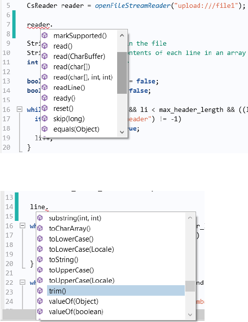
| 179

Note that you can see which additional methods are available for the reader

object by using Ctrl+Space, as shown in the figure below.

By using Ctrl+Space following a string, you can see the many additional methods

available for strings, including the

trim method used in the example above:

WRITING TEXT FILES USING THE CSWRITER CLASS

The example of the section “Reading Matrix Files” on page 172 uses an example

on the spreadsheet data format. This section contains an example that writes a file

on the sectionwise format, the other primary format in COMSOL Multiphysics for

saving postprocessing data. Data on the sectionwise format can, for example, be

read into an

Interpolation Curve geometry primitive. A file on the sectionwise

format may look like this:

% Version: COMSOL 5.4.0.123

% Date: May 5 2018, 8:00

% Description: Interpolation curve

% Coordinates

180 |

-1.1 -0.8

1.2 -0.9

0.9 1.3

-0.8 1.05

% Elements (segments)

1 2

2 3

3 4

The first few lines with comments start with the character % and are ignored when

imported as an

Interpolation Curve. The first section containing data starts on the

line after

% Coordinates. The second section containing data starts on the line

after

% Elements (segments). Note that the strings Coordinates and Elements

(segments)

are not necessary but each section containing data will be assumed to

start after each block of comments, regardless of what comes after the character

There may be additional blocks of data when, for example, exporting

Contour plot

data.

The following example code uses a

CsWriter stream to write interpolation curve

data to a text file. A template point set

p is copied in a circular pattern for a given

radius

R and number of copies n_of_copies.

CsWriter writer = openFileStreamWriter("temp:///my_curve.txt");

int n_of_copies = 10;

double[][] p = {{-1.2, -0.9}, {0.9, -1.1}, {1.3, 0.8}, {-0.9, 1.0}}; // template

int template_length = p.length;

double R = 10;

double px, py;

double pi = Math.PI;

String line;

int i1, i2;

String header =

"% Version:\tCOMSOL 5.4.0.123\r\n"

+"% Date:\tMay 5 2018, 8 : 00\r\n"

+"% Description:\tInterpolation curve\r\n"

+"% Coordinates:\r\n";

writer.append(header);

for (int j = 0; j < n_of_copies; j++) {

for (int i = 0; i < template_length; i++) {

px = p[i][0];

py = p[i][1];

px = px+R*Math.cos(2*pi*j/n_of_copies);

py = py+R*Math.sin(2*pi*j/n_of_copies);

line = toString(px)+

"\t"+toString(py)+"\r\n";

writer.append(line);

}

writer.append(

"% Elements (segments):\r\n");

for (int j = 0; j < n_of_copies; j++) {

| 181

for (int i = 0; i < template_length; i++) {

i1 = i+1;

i2 = (i+1)%template_length+1;

i1 = i1+j*template_length;

i2 = i2+j*template_length;

line = toString(i1)+

"\t"+toString(i2)+"\r\n";

writer.append(line);

}

writer.flush();

writer.close();

fileSaveAs(

"temp:///my_curve.txt");

Comments

The line

CsWriter writer = openFileStreamWriter("temp:///my_curve.txt");

opens a Java

character stream and assigns it to the object writer belonging to

the class

CsWriter.

The line

writer.append(header);

appends the contents of the string header to the (empty) file my_curve.txt.

The line

writer.flush();

writes the contents of the character stream buffer to file and empties the buffer but

does not close the stream permanently. At this point, you can still write more data

to the stream.

The line

writer.close();

closes the stream permanently. If you wish to write additional data to the file, you

have to open the stream again and append additional data.

182 |

Just as described above for the reader object, you can see which additional

methods are available for the

writer object by using Ctrl+Space, as shown in the

figure below.

You can import the resulting interpolation data as an

Interpolation Curve by

selecting the

Sectionwise option for Data format. This can be done for a 2D

geometry object or for a

Work Plane in 3D. The figure below shows the data

imported to a 2D model.

| 183

WRITING BINARY FILES

You write data to a binary file by using the methods of the class CsBinaryWriter

in a way that is somewhat similar to that of writing text using

CsWriter. However,

instead of writing strings and characters, you are writing bytes. To see how many

bytes each data type requires, see the table in the section “Primitive Data Types”

on page 8.

The example code below writes random 3D point data to a binary file. Each point

coordinate is stored as a

double and takes 8 bytes to store. The first 4 bytes of the

file stores the number of points in the file as an

int.

To conveniently convert between the regular data types, such as

double, int, and

byte arrays, the Java

library method java.nio.ByteBuffer is needed. This

method is not part of the standard methods available in the Method editor and

you need to use the fully qualified Java

class name java.nio.ByteBuffer, as

shown in the example code below.

byte[] bytes8 = new byte[8];

byte[] bytes4 = new byte[4];

CsBinaryWriter bwriter =

openBinaryFileStreamWriter(

"temp:///my_binary_file.dat");

int N = 1000;

java.nio.ByteBuffer.wrap(bytes4).putInt(N);

bwriter.write(bytes4);

double p[][] = new double[N][3];

for (int k = 0; k < N; k++) {

p[k][0] = Math.random();

java.nio.ByteBuffer.wrap(bytes8).putDouble(p[k][0]);

bwriter.write(bytes8);

p[k][1] = Math.random();

java.nio.ByteBuffer.wrap(bytes8).putDouble(p[k][1]);

bwriter.write(bytes8);

p[k][2] = Math.random();

java.nio.ByteBuffer.wrap(bytes8).putDouble(p[k][2]);

bwriter.write(bytes8);

bwriter.flush();

}

bwriter.close();

fileSaveAs(

"temp:///my_binary_file.dat");

Comments

The first two lines declare byte arrays of size 8 and 4, respectively

The line

CsBinaryWriter bwriter =

openBinaryFileStreamWriter(

"temp:///my_binary_file.dat");

opens a Java

byte stream.

The line

184 |

int N = 1000; // The number of points

denotes the number of points written to file.

The line

ByteBuffer.wrap(bytes4).putInt(N);

uses the imported ByteBuffer method to convert the integer N to a byte array

bytes4 of length 4.

The line

bwriter.write(bytes4);

writes the value of N to file.

The

for-loop creates N points and writes each x-, y-, and z-coordinate as doubles

using a byte array

bytes8 of length 8.

The line

bwriter.flush();

empties the byte buffer and the last two lines

bwriter.close();

fileSaveAs(

"temp:///my_binary_file.dat");

close the byte stream and display a file browser to the user to select a location to

save the binary file.

READING BINARY FILES

Based on the data format of the previous example, the code below reads a

corresponding binary file and plots the points as 3D point data.

byte[] bytes8 = new byte[8];

byte[] bytes4 = new byte[4];

CsBinaryReader breader = openBinaryFileStreamReader(

"upload:///file1");

breader.read(bytes4);

int N = java.nio.ByteBuffer.wrap(bytes4).getInt();

double p[][] = new double[N][3];

for (int k = 0; k < N; k++) {

breader.read(bytes8);

p[k][0] = java.nio.ByteBuffer.wrap(bytes8).getDouble();

breader.read(bytes8);

p[k][1] = java.nio.ByteBuffer.wrap(bytes8).getDouble();

breader.read(bytes8);

p[k][2] = java.nio.ByteBuffer.wrap(bytes8).getDouble();

}

breader.close();

| 185

double pt[][] = transpose(p);

String pgTag = model.result().uniquetag(

"pg");

ResultFeature pg = model.result().create(pgTag, 3);

ResultFeature plot = pg.create(

"pt1", "PointData");

plot.set(

"pointdata", pt);

plot.run();

useGraphics(model.result(pgTag),

"form1/graphics1");

Comments

The line

CsBinaryReader breader = openBinaryFileStreamReader("upload:///file1");

opens a Java

byte stream based on a File declaration file1, typically referenced

in a

File Browser form object, as in the earlier examples on reading text files.

The two lines

breader.read(bytes4);

int N = ByteBuffer.wrap(bytes4).getInt();

read the first 4 bytes and convert them to an int N.

The following

for-loop reads chunks of 8 bytes into the byte array bytes8,

converts them and stores the results in a 2D double array

The line

breader.close();

closes the byte stream.

The last section of the example code plots the data and is similar to the example

in “Reading Matrix Files” on page 172.

ADDITIONAL COMMENTS ON READING AND WRITING BINARY FORMATS

When processing binary files, there are two formats in which bytes can be stored:

little endian and big endian, respectively. By default, Java

uses the big endian

format. For example, the line

p[k][2] = ByteBuffer.wrap(bytes8).getDouble();

is the same as

p[k][2] = ByteBuffer.wrap(bytes8).order(ByteOrder.BIG_ENDIAN).getDouble();

In case the format you are reading is on the little endian format, the corresponding

line should be

p[k][2] = ByteBuffer.wrap(bytes8).order(ByteOrder.LITTLE_ENDIAN).getDouble();

186 |

Converting Interpolation Curve Data

The following method converts a geometry Interpolation Curve to an Interpolation

function (by creating an interpolation table). The method demonstrates extracting

geometry information from the underlying parameterization of an edge. The edge

doesn’t have to be an

Interpolation Curve but can be any single edge.

The curve is checked for being monotonous, which is required in order to be able

to convert to an interpolation function. Note that since an interpolation curve is

represented using splines, even though the interpolation points form a

monotonous sequence, the resulting curve may not; hence, the second consistency

check (the first check can potentially be skipped).

// Convert using N points

int N = 100;

double monoTol = 1e-6;

int edgeNum=1;

// Update and get geometry information

model.component("comp1").geom("geom1").run("fin");

GeomSequence geom1 = model.component("comp1").geom("geom1");

GeomFeature ic1 = geom1.feature("ic1");

double[][] curvePoints = ic1.getDoubleMatrix("table");

int len = curvePoints.length;

double minX = curvePoints[0][0];

double maxX = curvePoints[len-1][0];

double scale = maxX-minX;

double scaledTol = monoTol*scale;

| 187

for (int i = 1; i < len; i++) {

if ((curvePoints[i][0]-curvePoints[i-1][0]) < scaledTol) {

error("Curve needs to be a function curve with monotonously growing x

coordinates.");

}

double minMaxS[] = geom1.edgeParamRange(edgeNum);

double minS = minMaxS[0];

double maxS = minMaxS[1];

double sList[] = new double[N];

for (int k = 0; k < N; k++) {

sList[k] = (double) (N-1-k)/(double) (N-1)*minS+k/(double) (N-1)*maxS;

}

double[][] XY = geom1.edgeX(1, sList);

for (int j = 1; j < N; j++) {

if ((XY[j][0]-XY[j-1][0]) < scaledTol) {

error("Curve needs to be a function curve with monotonously growing x

coordinates.");

}

// Create interpolation table

model.func().create("int1", "Interpolation");

with(model.func("int1"));

set("funcname", "int1");

set("interp", "cubicspline");

set("extrap", "linear");

endwith();

model.func("int1").set("table", toString(XY));

Comments

The method assumes that there is a geometry sequence geom1 with an

interpolation curve

ic1. It further assumes that there are no other geometry

features and that the geometry object has a single edge. The integer

N determines

how granular the interpolation table should be. It is assumed that there is only one

edge in the geometry sequence (

edgeNum). Note that the curve parameter range

may not be the unit interval (

minS does not have to be 0.0 and maxS does not have

to be

1.0). To run the method more than once, you can create a cleanup method

that contains the lines:

model.func().remove("int1");

model.result().remove("pg1");

for removing previously created model tree nodes.

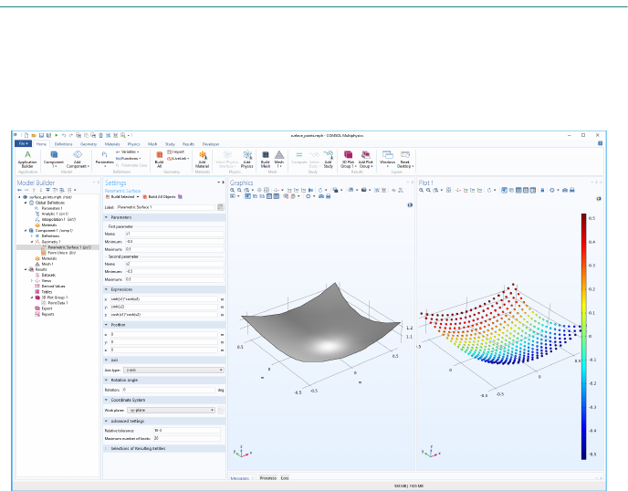
188 |

Plotting Points on a Parametric Surface

The following method retrieves coordinate values for a regularly sampled

parametric surface and plots the corresponding points using a

Point Data plot. The

method demonstrates extracting geometry information from the underlying

parameterization of a surface.

// Sample and plot N-by-N points on a parametric surface

int N = 20;

int faceNum = 1;

// Update and get geometry information

model.component("comp1").geom("geom1").run("fin");

GeomSequence geom1 = model.component("comp1").geom("geom1");

GeomFeature ps1 = geom1.feature("ps1");

double minMaxS[] = geom1.faceParamRange(faceNum);

double minS1 = minMaxS[0];

double maxS1 = minMaxS[1];

double minS2 = minMaxS[2];

double maxS2 = minMaxS[3];

double s1List[] = new double[N];

double s2List[] = new double[N];

for (int k = 0; k < N; k++) {

s1List[k] = (double) (N-1-k)/(double) (N-1)*minS1+k/(double) (N-1)*maxS1;

s2List[k] = (double) (N-1-k)/(double) (N-1)*minS2+k/(double) (N-1)*maxS2;

}

double s12List[][] = new double[N*N][2];

for (int i = 0; i < N; i++) {

| 189

for (int j = 0; j < N; j++) {

s12List[i+N*j][0] = s1List[i];

s12List[i+N*j][1] = s2List[j];

}

double[][] XY = geom1.faceX(faceNum, s12List);

// Plot points

String pgTag = model.result().uniquetag("pg");

ResultFeature pg = model.result().create(pgTag, 3);

ResultFeature plot = pg.create("pt1", "PointData");

double[][] p = new double[3][N*N];

double[] color = new double[N*N];

for (int i = 0; i < N*N; i++) {

p[0][i] = XY[i][0];

p[1][i] = XY[i][1];

p[2][i] = XY[i][2];

color[i] = p[1][i];

}

plot.set("pointdata", p)

.set("colordata", color)

.set("coloring", "colortable")

.set("sphereradiusscale", 1);

plot.run();

selectNode(pg);

Using Selections for Editing Geometry Objects

The following method generates a plate with an array of cylinders. The cylinders

may be used, for example, in a difference operation to create an array of holes in

the plate.

GeomSequence geom = model.component("comp1").geom("geom1");

geom.create("blk1", "Block");

geom.feature("blk1").set("size", new int[]{10, 10, 1});

geom.create("start_cyl1", "Cylinder");

geom.feature("start_cyl1").set("pos", new double[]{2.5, 2.5, 0});

geom.create("arr1", "Array");

geom.feature("arr1").selection("input").set("start_cyl1");

geom.feature("arr1").set("fullsize", new int[]{2, 2, 1});

geom.feature("arr1").set("displ", new int[]{5, 5, 0});

geom.run("arr1");

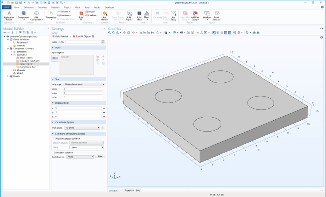
190 |

The resulting geometry is shown in the figure below.

Assume now that the resulting geometry, from the previous step, corresponds to

an imported geometry object and that you would like to replace the cylinders with

larger cylinders before subtracting and generating the holes. Furthermore, assume

that the cylinder objects are generated by an external software in such a way that,

although you know these objects are cylinders, they are represented as generic

geometry objects with no information on radius, height, or position. The

following method finds the array of cylinders, extracts coordinate information for

each cylinder, deletes the cylinders, creates a new array of wider cylinders, and

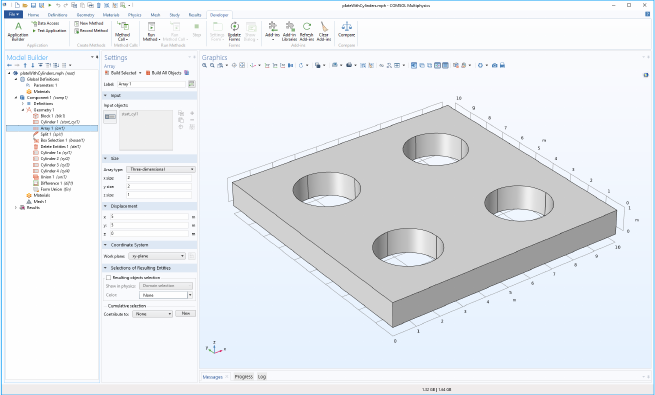
| 191

finally subtracts the cylinders from the plate. The resulting geometry is shown in

the figure below.

The method exemplifies retrieval of geometry object names, coordinate

information, and the use of selections. To start from another geometry object

(which is also necessarily a plate with cylinders), you can replace the string tag in

the variable

plateAndCylinders accordingly.

double selTol = 1e-2; // Selection tolerance

double newR = 1.25; // New cylinder radius

double newH = 1; // New cylinder height

double plateThickness = 1; // Plate thickness

String plateAndCylinders = "arr1";

// Update and split geometry

GeomSequence geom = model.component("comp1").geom("geom1");

geom.run(plateAndCylinders);

geom.create("spl1", "Split");

geom.feature("spl1").selection("input").set(plateAndCylinders);

geom.run("spl1");

// Find extents of geometry in x,y,z directions

double[] bBox = geom.getBoundingBox();

double MinX = bBox[0];

double MaxX = bBox[1];

double MinY = bBox[2];

double MaxY = bBox[3];

double MinZ = bBox[4];

double MaxZ = bBox[5];

// Define scaled coordinate tolerance

double scale = Math.max(Math.max(MaxX-MinX, MaxY-MinY), MaxZ-MinZ);

192 |

double scaleSelTol = scale*selTol;

// Create box selection based on geometry extents

geom.create("boxsel1", "BoxSelection");

with(geom.feature("boxsel1"));

// Select boundaries inside box in X-Y direction using tolerance

set("xmin", MinX+scaleSelTol);

set("xmax", MaxX-scaleSelTol);

set("ymin", MinY+scaleSelTol);

set("ymax", MaxY-scaleSelTol);

set("zmin", MinZ-scaleSelTol);

set("zmax", MaxZ+scaleSelTol);

set("condition", "inside");

set("entitydim", -1); // Select objects

endwith();

geom.run("boxsel1");

// Get object names

String[] so = geom.selection("boxsel1").objects();

int nso = so.length;

// Extract cylinder parameters

double[] MinXC = new double[nso];

double[] MaxXC = new double[nso];

double[] MinYC = new double[nso];

double[] MaxYC = new double[nso];

double[] MinZC = new double[nso];

double[] MaxZC = new double[nso];

double[] bBoxC = new double[6];

for (int i = 0; i < nso; i++) {

bBoxC = geom.obj(so[i]).getBoundingBox();

MinXC[i] = bBoxC[0];

MaxXC[i] = bBoxC[1];

MinYC[i] = bBoxC[2];

MaxYC[i] = bBoxC[3];

MinZC[i] = bBoxC[4];

MaxZC[i] = bBoxC[5];

}

double[] radius = new double[nso];

double[] xc = new double[nso];

double[] yc = new double[nso];

double[] zc = new double[nso];

double[] hc = new double[nso];

double ry;

double tol = scale*1e-6; // Tolerance check for skew cylinders, optional

consistency check

for (int i = 0; i < nso; i++) {

xc[i] = (MaxXC[i]+MinXC[i])/2;

yc[i] = (MaxYC[i]+MinYC[i])/2;

zc[i] = (MaxZC[i]+MinZC[i])/2;

hc[i] = MaxZC[i]-MinZC[i];

radius[i] = (MaxXC[i]-MinXC[i])/2;

ry = (MaxYC[i]-MinYC[i])/2;

if (Math.abs(radius[i]-ry) > tol)

| 193

error("Object is not a circular cylinder.");

}

// Delete all cylinder objects

geom.create("del1", "Delete");

geom.feature("del1").selection("input").init();

geom.feature("del1").selection("input").set(so);

geom.run("del1");

// Add new cylinders

String[] cylname = new String[nso];

for (int i = 0; i < nso; i++) {

cylname[i] = "cyl"+toString(i+1);

geom.create(cylname[i], "Cylinder");

with(geom.feature(cylname[i]));

set("r", newR);

set("h", newH+2*scaleSelTol);

set("pos", new double[]{xc[i], yc[i], plateThickness-2*zc[i]-scaleSelTol});

endwith();

}

// Combine all cylinders into one object

geom.create("uni1", "Union");

geom.feature("uni1").selection("input").set(cylname);

geom.run("uni1");

// Difference between all objects and cylinders

geom.create("dif1", "Difference");

String[] objs = geom.objectNames();

geom.feature("dif1").selection("input").set(objs);

geom.feature("dif1").selection("input2").set("uni1");

geom.run("dif1");

Comments

The method assumes that the input geometry objects have the same structure

as the plate with cylinders example above. Note that to clear the geometry

sequence, you can create a method with the line

model.component("comp1").geom("geom1").feature().clear();

This can be useful if you are running the main method from above repeatedly,

since you need to clear the geometry sequence before each run.

The first of the lines

geom.feature("del1").selection("input").init();

geom.feature("del1").selection("input").set(so);

initializes the selection to be empty of type object. The second line then selects all

objects with names in the array

so. In general, a call to init() without input

argument means that the selection is for objects and

init(n), where n=0,1,2, or

3, means that the selection is for points, edges, faces, and domains, respectively.

Note that in some cases

n=-1 is used to denote the object level (instead of an

empty input argument); see the Programming Reference Manual.

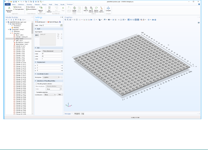
194 |

The figure below shows an example based on a larger array of cylinders.

Recursion and Recursively Defined Geometry Objects

Methods can support recursion by having a function calling itself in a recursive

loop. The following examples create recursive CAD geometry models of a

Sierpinski carpet in 2D and a Menger sponge in 3D.

Sierpinski Carpet

The following method, create_carpet, initiates the recursion to a certain

recursive level according to a user-defined

Parameter mslevel, defined under

Global Definitions in the Model Builder. It sets a limit at 5 levels in order to avoid

creating an exceedingly large geometry. The method assumes that you have

created a 2D Component and that you have declared an integer scalar variable

counter.

int level = (int) model.param().evaluate("mslevel");

if (level < 1)

error(

"Carpet level needs to be at least 1.");

if (level > 5)

error(

"Carpet level needs to be at most 5.");

counter = 0;

model.component(

"comp1").geom("geom1").feature().clear();

model.component(

"comp1").geom("geom1").autoRebuild("off");

double cx0 = 0, cy0 = 0;

double si0 = 1;

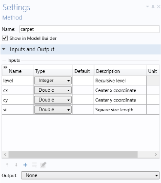
| 195

carpet(level, cx0, cy0, si0);

model.component(

"comp1").geom("geom1").runPre("fin");

The method create_carpet in turn calls the main recursive function carpet,

listed below, using four input arguments for the recursion level, the center x- and

y-coordinates, and the current side length.

The input arguments are defined in the method’s

Settings window, as shown

below.

The

code for the method carpet is shown below.

int l = level;

double posx, posy, si1;

String strix;

int l1;

for (int i = 0; i < 3; i++) {

for (int j = 0; j < 3; j++) {

posx = cx+i*si-si;

posy = cy+j*si-si;

strix = toString(i)+toString(j);

if ((Math.abs((i-1))+Math.abs((j-1))) > 0) {

if (l == 1) {

counter = counter+1;

model.component(

"comp1").geom("geom1").create("sq"+strix+"C"+toString(counter)

"Square");

with(model.component(

"comp1").geom("geom1").feature("sq"+strix+"C"+toString(co

unter)));

set(

"base", "center");

set(

"size", new double[]{si});

set(

"pos", new double[]{posx, posy});

endwith();

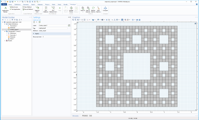
196 |

model.component(

"comp1").geom("geom1").feature("sq"+strix+"C"+toString(counter

)).label(

"Square"+strix+"C"+toString(counter));

} else {

l1 = l-1;

si1 = si/3;

carpet(l1, posx, posy, si1);

}

The figure below shows the resulting geometry for a level-3 carpet.

Note that the number of square geometry objects defined for the level 3 carpet is

512. The number of geometry objects for a level-N carpet is 8

. This means that

for the maximum level 5 set by the method

create_carpet, the resulting

geometry has 32,768 geometry objects.

Menger Sponge

The methods for the Sierpinski carpet readily generalize to 3D. However, in 3D,

you need to be careful not to generate more objects than your computer can

handle. The method assumes that you have created a 3D Component and that you

have declared an integer scalar variable

counter.

The following method,

create_sponge, initiates the recursion.

int level = (int) model.param().evaluate("mslevel");

if (level < 1)

error(

"Sponge level needs to be at least 1.");

if (level > 3)

error(

"Sponge level needs to be at most 3.");

| 197

counter = 0;

model.component(

"comp1").geom("geom1").feature().clear();

model.component(

"comp1").geom("geom1").autoRebuild("off");

double cx0 = 0, cy0 = 0, cz0 = 0;

double si0 = 1;

sponge(level, cx0, cy0, cz0, si0);

model.component(

"comp1").geom("geom1").runPre("fin");

The method sponge, shown below, is called by the above method and recursively

creates a Menger sponge.

int l = level;

double posx, posy, posz, si1;

String strix;

int l1;

for (int i = 0; i < 3; i++) {

for (int j = 0; j < 3; j++) {

for (int k = 0; k < 3; k++) {

posx = cx+i*si-si;

posy = cy+j*si-si;

posz = cz+k*si-si;

strix = toString(i)+toString(j)+toString(k);

if ((Math.abs((i-1))+Math.abs((j-1))+Math.abs((k-1))) > 1) {

if (l == 1) {

counter = counter+1;

model.component(

"comp1").geom("geom1").create("blk"+strix+"C"+toString(counter

"Block");

with(model.component(

"comp1").geom("geom1").feature("blk"+strix+"C"+toString(c

ounter)));

set(

"base", "center");

set(

"size", new String[]{toString(si), toString(si), toString(si)});

set(

"pos", new double[]{posx, posy, posz});

endwith();

model.component(

"comp1").geom("geom1").feature("blk"+strix+"C"+toString(counte

r)).label(

"Block"+strix+"C"+toString(counter));

} else {

l1 = l-1;

si1 = si/3;

sponge(l1, posx, posy, posz, si1);

}

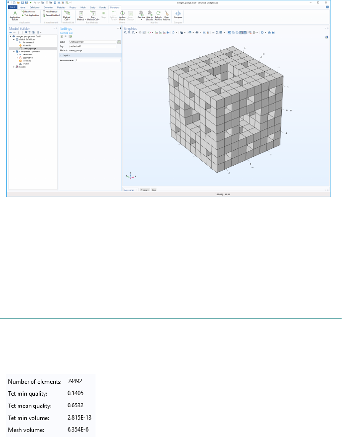
198 |

The figure below shows the resulting geometry for a level-2 sponge.

In this case, the number of geometry objects grows with the level N as 20

and

the level-2 sponge shown above has 400 block geometry objects.

Note that if you have any of the add-on products for additional CAD

functionality, you can export these geometry objects on standard CAD formats.

Without add-on products, you can export the meshed geometry to any of the

supported mesh formats.

Mesh Information and Statistics

You can retrieve a variety of mesh information and statistics quantities, such as

element quality, the total number of elements, mesh volume, and so on. The

figure below shows part of an application displaying such information.

Assuming that you would like to link the various mesh quantities to variables

declared under the

Declarations node, the corresponding method code would

include the following lines of code:

| 199

a = model.component("comp1").mesh("mesh1").getNumElem();

b = model.component(

"comp1").mesh("mesh1").getMinQuality("tet");

c = model.component(

"comp1").mesh("mesh1").getMeanQuality("tet");

d = model.component(

"comp1").mesh("mesh1").getMinVolume("tet");

e = model.component(

"comp1").mesh("mesh1").getVolume("tet");

For more information on available mesh quantities, see the Reference Manual.

Accessing Higher-Order Finite Element Nodes

The extended mesh data structure contains information related to the finite

element method including, for example, the placement of higher-order element

nodes. The extended mesh information is contained in the class

XmeshInfo and

provides information about the numbering of elements, nodes, and degrees of

freedom (DOFs) in the extended mesh and in the matrices returned by the

Assemble feature and the solvers. For detailed information on XmeshInfo, see the

Programming Reference Manual.

The following example method illustrates how to use the extended mesh

information to plot higher-order nodes in a few important special cases. The

example covers cases with one model component, one geometry, and a subset of

physics combinations. If you apply it to other cases, you will get an error message.

// Note that this method is only implemented for one component and one geometry

and doesn't work for all physics combinations.

String stdTag = model.study().uniquetag(

"stdfe");

model.study().create(stdTag);

model.study(stdTag).label(

"FE Nodes Study "+stdTag.substring(5));

model.study(stdTag).showAutoSequences(

"sol");

String solTag = model.sol().uniquetag(

"sol");

model.sol().create(solTag);

model.sol(solTag).create(

"st1", "StudyStep");

model.sol(solTag).create(

"v1", "Variables");

SolverFeature step = model.sol(solTag).feature(

"v1");

XmeshInfo xmi = step.xmeshInfo();

try {

XmeshInfoNodes testnodes = xmi.nodes();

} catch (Exception e) {

error(

"Cannot access finite element data. Only implemented for one geometry and

stationary studies.

");

}

XmeshInfoNodes mynodes = xmi.nodes();

double[][] coords = mynodes.gCoords();

int[] coordsize = matrixSize(coords);

int sdim = 0;

if (coordsize[0] == 3) {

200 |

sdim = 3;

} else if (coordsize[0] == 2) {

sdim = 2;

} else

error(

"The geometry of the first component is not 2D or 3D.");

String mesh =

"mesh"+stdTag;

model.result().dataset().create(mesh,

"Mesh");

String pgTag = model.result().uniquetag(

"pgfe");

ResultFeature pg = model.result().create(pgTag, sdim);

model.result(pgTag).label(

"FE Nodes Plot "+pgTag.substring(4));

String nodes = pgTag;

model.result(nodes).create(

"mesh", "Mesh");

if (sdim == 3) {

with(model.result(nodes).feature(

"mesh"));

set(

"data", mesh);

set(

"meshdomain", "volume");

endwith();

} else {

with(model.result(nodes).feature(

"mesh"));

set(

"data", mesh);

set(

"meshdomain", "surface");

endwith();

}

with(model.result(nodes).feature(

"mesh"));

set(

"elemcolor", "none");

set(

"wireframecolor", "gray");

set(

"elemscale", 0.999);

endwith();

with(model.result(nodes));

set(

"edges", true);

set(

"data", mesh);

endwith();

ResultFeature plot = pg.create(

"pt1", "PointData");

plot.set(

"pointdata", coords)

.set(

"coloring", "uniform")

.set(

"color", "red");

plot.run();

selectNode(pg);

Comments

The first few lines of the method set up a solver step object step, which is used to

extract the extended mesh information. The extended mesh information, which

contains information on the higher-order nodes, is extracted in the line

XmeshInfo xmi = step.xmeshInfo();

The lines

XmeshInfoNodes mynodes = xmi.nodes();

double[][] coords = mynodes.gCoords();

| 201

int[] coordsize = matrixSize(coords);

access and store the finite element node coordinates in a 2-by-coordsize (2D) or

3-by-coordsize (3D) array.

The following code segments set up a mesh data set and an associated mesh plot.

The last section uses the low-level

PointData plot type to visualize the finite

element nodes. For more information on this plot type, see “Points in 3D” on

page 153.

Accessing System Matrices and Vectors

You can gain low-level access to the finite element system matrices and vectors by

adding nodes of the types Assemble and Input Matrix under a Study node.

The example below shows how to set up and solve a 2D electrostatics problem on

the unit square [0,1]-by-[0,1]. After the original problem is solved, the load

vector is modified at a user-defined coordinate. The code searches for the degree

of freedom closest to the target user-defined coordinate and modifies the load

vector to a user-defined value. The physical interpretation of the modified load is

that of an added volume charge.

To run the example code below, first use the Model Wizard to create a blank

model. Then, add a new method and paste the example code below. Finally, run

the method. You can try changing the variable values in the Initializations section

at the beginning of the code and run again.

// Initializations

double x_load = 0.2; // Target x-coordinate for load

double y_load = 0.2; // Target y-coordinate for load

double load = 1e-9; // Load, volume charge

double dist = 10.0; // Distance to (x_load,y_load) from degree of freedom

int index = 0; // Index of the degree of freedom closest to (x_load,y_load)

// Clear any previous model.

clearModel(model);

// Create a new model component.

model.modelNode().create(

"comp1");

// Create the 2D geometry.

model.geom().create(

"geom1", 2);

model.geom(

"geom1").feature().create("sq1", "Square");

model.geom(

"geom1").run();

// Create the mesh.

model.mesh().create(

"mesh1", "geom1");

model.mesh(

"mesh1").feature().create("fre1", "FreeTri");

model.mesh(

"mesh1").run();

202 |

// Setup the electrostatics physics problem.

model.physics().create(

"es", "Electrostatics", "geom1");

model.physics(

"es").feature().create("gnd1", "Ground", 1);

model.physics(

"es").feature("gnd1").selection().set(new int[]{1});

model.physics(

"es").feature().create("sfcd1", "SurfaceChargeDensity", 1);

model.physics(

"es").feature("sfcd1").selection().set(new int[]{4});

// Add a varying distributed charge density along the rightmost boundary.

model.physics(

"es").feature("sfcd1").set("rhoqs", "1e-9*y");

model.component(

"comp1").physics("es").feature("ccn1").set("epsilonr_mat",

"userdef");

model.component(

"comp1").physics("es").feature("ccn1").set("epsilonr", "1");

// Change to 1st order shape functions, to keep things simple.

model.component(

"comp1").physics("es").prop("ShapeProperty").set("order_electr

icpotential

", 1);

// Create and run the study.

model.study().create(

"std1");

model.study(

"std1").feature().create("stat1", "Stationary");

model.study(

"std1").run();

// Create a 2D plot group with a surface plot for the original problem.

model.result().create(

"pg1", 2);

model.result(

"pg1").set("data", "dset1");

model.result(

"pg1").feature().create("surf1", "Surface");

selectNode(model.result(

"pg1")); // Set focus on the plot node.

// Create a reusable solver feature variable.

SolverFeature solft;

model.study().create(

"std2"); // Create a Study 2 node.

model.sol().create(

"sol2"); // Create a data set Solution 2.

// Create a Solver configurations node under Study 2

model.sol(

"sol2").study("std2");

model.sol(

"sol2").create("st1", "StudyStep"); // Create a Compile Equations

node.

solft = model.sol(

"sol2").feature("st1"); // Assign solver step to variable

solver.

solft.set(

"study", "std2");

model.sol(

"sol2").create("v1", "Variables"); // Create a Dependent Variables

node.

solft = model.sol(

"sol2").feature("v1");

model.sol(

"sol2").attach("std2");

model.sol(

"sol2").create("a1", "Assemble"); // Add an Assemble node.

solft = model.sol(

"sol2").feature("a1");

// Now define which system matrices should be output (Non-Eliminated Output).

// L=Load vector, K=Stiffness matrix, M=Constraint vector, N=Constraint Jacobian

// For more information see the Programming Reference Manual.

solft.set(

"L", "on");

solft.set(

"K", "on");

solft.set(

"M", "on");

solft.set(

"N", "on");

| 203

//Create a Stationary Solver 2 node: Study 2>Solver Configurations>Solution 2.

model.sol(

"sol2").create("s2", "Stationary");

// Create an Input Matrix node under Stationary Solver 2.

solft = model.sol(

"sol2").feature("s2").create("im1", "InputMatrix");

// Define which system matrices should be input.

solft.set(

"L", "on");

solft.set(

"K", "on");

solft.set(

"M", "on");

solft.set(

"N", "on");

// Find the degree of freedom coordinate closest to the target coordinate.

solft = model.sol(

"sol2").feature("v1");

XmeshInfo xmi = solft.xmeshInfo();

XmeshInfoDofs mydofs = xmi.dofs();

double[][] coords = mydofs.gCoords();

int[] coordsize = matrixSize(coords);

double new_dist = dist;

for (int k = 0; k < coordsize[1]; k++) {

new_dist =

Math.sqrt((coords[0][k]-x_load)*(coords[0][k]-x_load)+(coords[1][k]-y_load)*(co

ords[1][k]-y_load));

if (new_dist < dist) {

index = k;

dist = new_dist;

}

// Run the solver sequence up to and including the Assemble node.

model.sol(

"sol2").runFromTo("st1", "a1");

// Extract system matrices and vectors.

solft = model.sol(

"sol2").feature("a1");

// K

int KM = solft.getM(

"K");

int KN = solft.getN(

"K");

int KNnz = solft.getNnz(

"K");

int[] Ki = solft.getSparseMatrixRow(

"K");

int[] Kj = solft.getSparseMatrixCol(

"K");

double[] Kv = solft.getSparseMatrixVal(

"K");

// For more information, see the Programming Reference Manual.

// L

double[] Lv = solft.getVector(

"L");

// N

int NM = solft.getM(

"N");

int NN = solft.getN(

"N");

int NNnz = solft.getNnz(

"N");

int[] Ni = solft.getSparseMatrixRow(

"N");

int[] Nj = solft.getSparseMatrixCol(

"N");

double[] Nv = solft.getSparseMatrixVal(

"N");

// M

double[] Mv = solft.getVector(

"M");

204 |

// Modify the load

Lv[index] = load;

// Put the system matrices and vectors back in again.

solft = model.sol(

"sol2").feature("s2").feature("im1");

// K

solft.createSparseMatrix(

"K", KM, KN, KNnz, true);

solft.addSparseMatrixVal(

"K", Ki, Kj, Kv);

// L

solft.createVector(

"L", Lv.length, true);

solft.setVector(

"L", Lv);

// N

solft.createSparseMatrix(

"N", NM, NN, NNnz, true);

solft.addSparseMatrixVal(

"N", Ni, Nj, Nv);

// M

solft.createVector(

"M", Mv.length, true);

solft.setVector(

"M", Mv);

// Solve Stationary Solver 2 with the modified system.

model.sol(

"sol2").runFromTo("s2", "s2");

// Plot the results.

model.result().create(

"pg2", "PlotGroup2D");

with(model.result(

"pg2"));

set(

"data", "dset2");

endwith();

model.result(

"pg2").create("surf1", "Surface");

// Plot electric potential and original mesh overlayed with no smoothing.

with(model.result(

"pg2").feature("surf1"));

set(

"resolution", "norefine");

set(

"smooth", "none");

endwith();

model.result(

"pg2").create("surf2", "Surface");

with(model.result(

"pg2").feature("surf2"));

set(

"resolution", "norefine");

set(

"coloring", "uniform");

set(

"color", "gray");

set(

"wireframe", true);

endwith();

model.result(

"pg2").run();

selectNode(model.result(

"pg2")); // Set focus on the plot node.

Comments

In the previous example, “Accessing Higher-Order Finite Element Nodes” on

page 199, the

XmeshInfoNodes methods are used to access finite element nodes

that have the same length as the number of finite element nodes. In this example,

the

XmeshInfoDofs methods are used to access the degrees of freedom vector,

which has the same length as the load vector.

| 205

Note that only the load vector is modified. The other matrices and vectors are

merely extracted and then put back into the system again.

Using Built-In Methods from an External Java Library

When developing an external Java

library to be used in the Application Builder,

it is possible to call the built-in methods from the external library. In order to do

so, the

com.comsol.api JAR-file needs to be added to the project build path, and

the classes that call the methods need to extend the

ApplicationLanguageBase

class. The following steps explain how to create a simple example JAR library when

using the Eclipse

integrated development environment:

1 Start Eclipse

2 Create a new Java

project. Enter JavaLibDemo as the project name and click

Next.

3 Go to the

Libraries tab and click Add External JARs. Add the JAR-file

com.comsol.api_1.0.0.jar from the plugins directory under the COMSOL

Multiphysics installation directory; for example

C:\Program Files\COMSOL\COMSOL54\Multiphysics\plugins

4 Click Finish.

5 Right-click the

src folder in your Eclipse project and select New... Package. Enter

demo as the package name and click Finish.

6 Right-click the

demo package in your Eclipse project and select New... Class. Enter

Hello as the class name.

7 Click on

Superclass > Browse... and select ApplicationLanguageBase. Click OK

and

Finish.

8 In the editor window for the

Hello class, add the following method and save

the file:

public static void hello() {

alert(

"Hello!");

}

9 Right-click the JavaLibDemo project and select Export... > Java > JAR file. Select

the export destination JAR-file and click

Finish.

10 Start COMSOL Multiphysics and create a

Blank Model.

11 In the Application Builder, under the application tree, right-click

Libraries and

select

External Java Library. In the Settings window, click Browse... and select the

JAR-file previously exported from Eclipse

12 In the Application Builder, add a form, button, and method for the button.

206 |

13 In the Method editor for the method, add the following code:

Hello.hello();

14 Click Test Application and click the button in the application to verify that the

alert method is invoked.

Measuring the Java Heap Space Memory

Software components that are based on Java

, such as certain parts of COMSOL

Multiphysics, are predefined to use only a limited amount of memory. This limit,

the Java

heap space, is specified during startup. Note that the Java

heap space

only affects certain parts of the software and not, for example, meshing or solvers.

By default, COMSOL Multiphysics allocates 2 GB of Java

heap space memory.

See the Reference Manual for information about increasing the available heap

space memory.

In a method, you can measure the amount of heap space memory currently in use.

For example, while debugging, you can add the following code:

Runtime runtime = java.lang.Runtime.getRuntime();

runtime.gc();

debugLog("Used memory (MB):

"+(runtime.totalMemory()-runtime.freeMemory())/(1024*1024));

The first line adds a request to run the Java

garbage collector.

In order to monitor the memory usage in an application, you can replace

debugLog with message.

Time-Limited and Hardware-Locked Applications

By writing a few lines of code, you can make your application expire after a set date

and lock the application to specific hardware.

The example MPH-file used in this section is available in the Application

Gallery at https://www.comsol.com/model/70151

PASSWORD PROTECTION

The settings of an application can in principle be read from the file system by a

user, including method code. By making your application password protected for

editing, the method code will no longer be readable. This setting is available from

the root node in either the model tree or the application tree, as shown in the

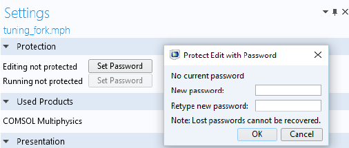
| 207

figure below.

Before implementing a time limit or hardware lock, as described below, make sure

your application is password protected. Password protection for running the

application is not required for this purpose.

TIME-LIMITED APPLICATION

To have an application expire after a specific date, create a method as follows:

java.text.SimpleDateFormat f = new java.text.SimpleDateFormat("yyyy-MM-dd");

//java.text.SimpleDateFormat f = new java.text.SimpleDateFormat("MM/dd/yyyy");

ok = false;

try {

java.util.Date d = f.parse(timeoutDate);

long currentTime = timeStamp();

long timeoutTime = d.getTime()+24*60*60*1000; // To allow running until the end

of the day

if (currentTime < timeoutTime) {

ok = true;

}

catch (java.text.ParseException e) {

debugLog("Failed to parse timeout date "+timeoutDate);

debugLog(e.getMessage());

}

In this method, you need to decide on a date format. Two format examples are

shown and you can uncomment the line corresponding to the format you would

like to use. For more details on available formats, see the Java

documentation for

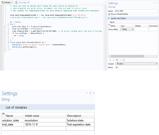
208 |

SimpleDateFormat. This method has one string input argument, timoutDate,

and one Boolean output argument,

ok, as shown below.

The expiration date is defined as a string variable,

trial_date, in

Declarations>String, as shown below.

HARDWARE-LOCKED APPLICATION

To lock an application to the MAC address of a specific network card on a

computer, create a method as follows:

ok = false;

try {

java.util.List < java.net.NetworkInterface > nis =

java.util.Collections.list(java.net.NetworkInterface.getNetworkInterfaces());

for (java.net.NetworkInterface ni : nis) {

StringBuilder macString = new StringBuilder();

byte[] macBytes = ni.getHardwareAddress();

if (macBytes != null && macBytes.length > 0) {

for (byte b : macBytes) {

if (macString.length() > 0) {

macString.append(":");

}

macString.append(String.format("%02x", b));

}

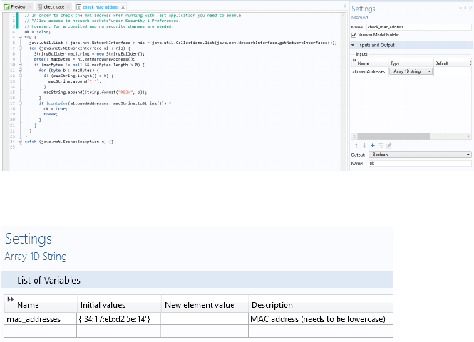
| 209

if (contains(allowedAddresses, macString.toString())) {

ok = true;

break;

}

catch (java.net.SocketException e) {}

In order to check the MAC address when running an application, you need to

enable

Allow access to network sockets under Security in Preferences. However, for

a compiled application, no security changes are needed.

This method has one array 1D string input argument,

allowedAddresses, and

one Boolean output argument,

ok, as shown below.

The MAC address is defined as a string array

mac_addresses in Declarations>Array

1D String

, as shown below.

Note that you can provide a list of MAC addresses to allow use on a computer with

multiple network cards or multiple computers.

CHECKING FOR ALLOWED DATE AND HARDWARE

To check for both the MAC address and the date, create a method

check_allowed_to_run as follows:

if (!check_mac_address(mac_addresses)) {

alert("You are not allowed to run this application on this computer.",

"COMSOL");

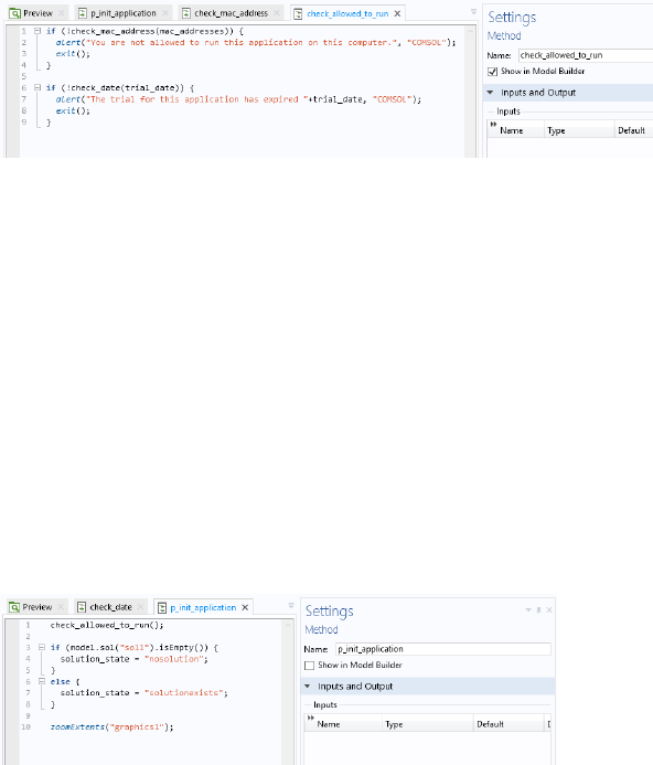
210 |

exit();

}

if (!check_date(trial_date)) {

alert("The trial for this application has expired "+trial_date, "COMSOL");

exit();

}

The figure below shows this method in the Method editor.

You can call this type of method at startup of the application, for example, as an

On load event for the main form of the application. In the Tuning Fork example

application, available in the Application Library of COMSOL Multiphysics, there

is a method

p_init_application that is run as an On load event for the main

form. In this case, the method

p_init_application can be edited as follows:

check_allowed_to_run();

if (model.sol("sol1").isEmpty()) {

solution_state = "nosolution";

}

else {

solution_state = "solutionexists";

}

zoomExtents("graphics1");

Notice the call to the method check_allowed_to_run in the first line. The figure

below shows this method in the Method editor.

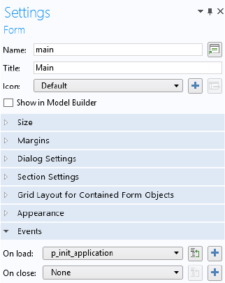
| 211

The method p_init_application is then called as an On load event. This is

specified in the

Settings window of the main form, as shown in the figure below.

212 |

| 213

Index

1D array 12, 31, 136

2D array 13, 31, 136

A accessing 201

add-in 23, 148

alert 112, 118

anisotropic diffusion coefficient 33

Annotation Data plot type 161

Application Builder 55

Application Builder Reference Manual

124

application example

tubular reactor

110

application object 7, 25, 55, 91

app variable 57

classes 57

application tree 55

array 12

methods 136

array 1D

object

array 2D

object

array input object 65

Arrow Data plot type 159, 160

assignments 8

auto complete 18

automatic solver sequence 47

axisymmetric property 29

B backslash 12

backspace 12

basic data type 29

big endian 185

binary file

processing

185

reading 184

writing 183

Blank Model 29

boolean

data type

8, 29

Boolean variable 8

conversion 134

boundary condition 41

built-in method library 91

button

object

C C libraries

external

123

card stack object 66

carriage return 12

catch 17

C-code

linking

123

char

data type

character

data type

character stream 178

characters

special

177

check box object 66

choice list 57, 86, 116

methods 86

object 84

classes

application object

code completion 18

code generation 18

collection methods 145

color 59

of user interface component 58

214 |

combo box object 67

Compact History 52

Compile Equations node 45

computation time 133

last 132

Compute 46

COMSOL Desktop 51

COMSOL Help Desk 53

COMSOL Multiphysics 7, 25

confirm 11, 112, 118

contour plot 48

contour plot data 180

control flow statements 15

conversion

between data types

methods 134

coordinate information 190, 191

Copy as Code to Clipboard 29

creating

feature node

37, 41

model object 28, 51

CSV-file 162, 170

curve

interpolation

179

parameterization 186

cut point

data set

33, 92

D data display object 68

data set 48, 151

Data Source

class

57, 84

data types

primitive

date and time methods 131

debug

methods

123

Debug Log window 123

declaration

type

Declarations 12, 14, 56

deformation plot 34

degrees of freedom 199

Dependent Variables node 45

description 17

parameter 17, 34

variable 17

Developer tab 150

dialog box 111, 112

diffusion coefficient

anisotropic

dimension

spatial

disable form object 59, 63, 64, 116

Display Name

for choice list

116

double 9

data type 8, 29

variable conversion 134

double quotation mark 11

E edge

parameterization

186

Editor Tools window 35

Electric Currents 50

element

order

199

size 32, 39

elementary math functions 15

class

107

methods 107

preferences 109

email attachment

export

107

report 107

table 107

embedded model 51

enable form object 57, 59, 63, 64, 116

endian 185

| 215

equation

object

error dialog box 17

example code 91, 150

Excel® file 49, 100, 162, 167, 171

exception

handling

exit 122

application 122

expiration date for application 206

export

email attachment

107

external C libraries 123

external Java® library 205

F face

parameterization

188

feature node

creating

37, 41

removing 38, 41

file

methods

name 100

open 103

reading 162

writing to 162

File Declaration 165

file import 165

file import object 69

file open

system method

103

file scheme

syntax

96, 165

finite element

accessing

199

system matrix 201

vector 201

floating point number 8

for loop 16, 64, 90

form

class

58, 62

declarations 14

list methods 89

form collection 70

form method 23

form object 69

class 58, 63

list methods 89

types 64

formfeed 12

Fully Coupled node 46

G general properties 59

generating code 18

Geometry node 37

geometry object 37, 38

names 191

get 29

global method 23

global parameter 34

graphics

object

70, 111

grid data set 150

GUI command

methods

122

GUI related methods 111

H hardware lock 206

heap space 206

Heat Transfer in Solids 40, 50

higher-order element nodes 199

history

model

HTML

report

119

hyperlink object 71

I if-else statement 15

image object 72

import

216 |

file 165

information card stack object 72

information node 133

inherit

color

input field object 73

integer

data type

8, 29

variable conversion 134

interpolation curve 179, 186

interpolation function 186

Introduction to Application Builder 7,

18, 22, 23, 55, 87, 96, 133, 162

Introduction to COMSOL Multiphysics

22, 25

isosurface 150

item

class

list methods 89

menu 83

object 83

ribbon 83

toolbar 83

iterative solver 45

Iterator class and method 41

J jagged arrays 12

Java

Documentation, model object class

structure

math library 15

programming language 7, 8, 91

syntax 9

unary and binary operators 9

Java®

character stream

178

classes for read/write 177

external library 205

heap space 206

K keyboard shortcut

Ctrl+Space

L legend 33, 34

license

check out

123

method 93

lighting 157

Line Data plot type 154

line object 75

list box object 75

literals 8

little endian 185

load vector 204

model

51, 92

local method 23

locking application to hardware 206

log object 76

looplevel property 49

M MAC address 206

main application class 57, 60

main user interface component classes

Main Window

class

58, 61

node 58

material

link

tag 87

Materials node 42

math functions 15

maximum value 49

item

mesh

information and statistics

198

mesh element size 32, 39

Mesh node 39

| 217

message log object 76, 114

message method 118

method 7, 91

form 23

get 29

global 23

local 23

name 24

Method class 89

Method editor 91

using 7, 18

method name 24

Microsoft® Word® format 119

model 51

loading 51, 92

saving 51, 92

Model Builder 25

model component 28

model data access 22

model history 52, 153

recording 52

turning off 153

Model Java-file 52

Model M-file 52

model object 7, 25, 42, 55, 91

class structure 53

tag 25

model tag 28

model tree 25

node 41, 42

model utility methods 52, 91

Model Wizard 29, 51

models, working with multiple 51

MPH file 51, 91, 122

multiphysics 50

Multiphysics node 50

multiple models 51

N name

form

55, 57

form object 55, 57

in application object 57

method 24

scoping 27

shortcut 14, 55

user interface component 55, 57

network card 206

newline 11, 12

node

finite element

199

nonlinear solver 46

normal

surface

157, 158

numerical

Derived Values

O operating system

methods

103

operators 36

Java 9

model object 36

OS commands 103

P parameter 17, 33, 34, 49

method 16, 23

real and imaginary part 35

parameterization

edge

186

face 188

parameterized solution 49

parsing

text file

177

physics interface 40, 44

play sound 104

plot

group

34, 118

mesh element nodes 92

point trajectories 92

surface 37, 48

table surface 49

218 |

useGraphics 111

Plot Group node 48

plot type

Annotation Data

161

Arrow Data 159, 160

Line Data 154

Point Data 152, 153, 201

Surface Data 155, 156, 157

Tube Data 159

Point Data plot type 152, 153, 201

point trajectories plot 92

precedence, of operators 9, 36

primitive data types 8

printing

graphics

122

programming examples 91, 150

Programming Reference Manual 25, 47,

91, 92, 193, 199

progress 125

dialog box 126, 130

methods 125

progress bar object 76, 127, 129, 130

properties

general

property and property values 29

R radio button object 77

ragged arrays 12, 32

reading

binary file

184

CSV-file 163

Excel® file 167

file 162

matrix file 172

Microsoft Excel® Workbook file 167

spreadsheet 163

text file 177

text file to string 174

real and imaginary part

of parameter

Record Code 20, 46

recursion 194

recursive loop 194

Reference Manual 199

removing

feature node

38, 41

report 110

email attachment 107

HTML 119

Microsoft® Word® format 119

request 113, 118

reset

model history

Results node 48

results table object 77, 115

RGB color 60

ribbon item 83

S save application 122

save as 122

saving

model

51, 92

scalar

object

scene light 122

sectionwise

format

179, 182

sectionwise format 179

selection input

object

selections 191

set 29

setIndex 29

shortcuts 14, 55

Shortcuts node 14

single quotation mark 11

sleep 133

slider object 79

SMTP 109

solution

| 219

data 150

data structure 45

parameterized 49

Solution node 45

Solver Configurations node 44

solver sequence 44

spacer object 79

spatial dimension 28

special character 11

Java 52

special characters 177

sphere 150

spreadsheet 163

format 96, 172, 173, 179

Stationary Solver node 45

Stationary study step 44

status bar 125

stream

character

178

String

data type

10, 29

methods 144

string variable 49

conversion 135

methods 144

strings

comparing

concatenating 10

Study node 44

subform object 69

surface

parameterization

188

Surface Data plot type 155, 156, 157

surface normal 157, 158

surface plot 37, 48

system matrix

accessing

201

system methods 103

OS commands 103

system vector 201

T tab 12

table 49

email attachment 107

object 80, 114

Table node 49

table surface plot 49

tag 57

model 28

model object 25

physics interface 40

temporary folder

location

171

text file 162

reading 177

writing 177

text label object 81

text object 80

time 131

time-limited application 206

title 112

toggle button object 81

toolbar

item

object 82

transparency 120, 122

transparent

color

try and catch 17

Tube Data plot type 159

type declaration 54

U unit 35

object 82

Unit List 57

unit set

methods

object 84

unit sphere 150

220 |

Unit System 35

username 103

V variable 23

description 17

name completion 19

video object 82

view

graphics

117, 119

visualization 150

W web page object 83

while loop 16

with statement 16

writing

CSF-file

170

Excel file 171

matrix file 173

string to text file 176

text file 177

to binary file 183

to file 162, 171

Z zoom extents 118, 122