Bank Funding Risk, Reference Rates, and Credit Supply

Bank Funding Risk,

Reference Rates, and

Credit Supply

Harry Cooperman | Darrell Duffie | Stephan Luck |

Zachry Wang | Yilin (David) Yang

NO. 1042

DECEMBER 2022

REVISED

FEBRUARY 2023

Bank Funding Risk, Reference Rates, and Credit Supply

Harry Cooperman, Darrell Duffie, Stephan Luck, Zachry Wang, and Yilin (David) Yang

Federal Reserve Bank of New York Staff Reports, no. 1042

December 2022; revised February 2023

JEL classification: G00, G01, G02, G20, G21, E4, E43

Abstract

Corporate credit lines are drawn more heavily when funding markets are more stressed. This covariance

elevates expected bank funding costs. We show that credit supply is dampened by the associated debt-

overhang cost to bank shareholders. Until 2022, this impact was reduced by linking the interest paid on

lines to credit-sensitive reference rates such as LIBOR. We show that transition to risk-free reference

rates may exacerbate this friction. The adverse impact on credit supply is offset if drawdowns are

expected to be left on deposit at the same bank, which happened at some of the largest banks during the

COVID recession.

Key words: bank funding risk, credit supply, reference rates, credit lines, London Interbank Offered Rate

(LIBOR), Secured Overnight Financing Rate (SOFR)

_________________

Luck: Federal Reserve Bank of New York (email: [email protected]). Cooperman, Duffie, Wang:

Stanford Graduate School of Business (emails: [email protected], [email protected],

[email protected]). Yang: City University of Hong Kong (email: yiliy[email protected]). The

authors thank discussants Anne Duquerroy, Dan Greenwald, David Glancy, Anil Kashyap, Elie Lewi,

Jose-Luis Peydro, and Peter Zimmermann, as well as Alena-Kang Landsberg for her excellent research

assistance. The authors are also grateful for conversations with Gara Afonso, Yacov Amihud, Leif

Andersen, Viral Acharya, Roc Armenter, Tom Baxter, Antje Berndt, Alastair Borthwick, Tim Bowler,

Laurent Clerc, Natalie Cox, Tom Deas, Fulvia Fringuelotti, Jason Granet, Vivien Lévy-Garboua, Andrei

Magasiner, John Marynowski, Bill Nelson, Peter Phelan, Michael Roberts, Richard Sandor, Gagan Singh,

Jeremy Stein, Jonathan Wallen, and Nathaniel Wuerffel, as well as seminar and conference participants at

the Federal Reserve Bank of New York, Stanford University, NYU Stern, Wharton, the Federal Reserve

Bank of San Francisco, the Financial Stability Conference at the Federal Reserve Bank of Cleveland,

System Committee on Financial Institutions, Regulation, and Markets held at the Federal Reserve Bank

of Kansas City, ES European Winter Meeting 2022, EFA 2022, AFA 2023 in New Orleans, Banque de

France, Symposium on Private Firms at University of Chicago, and Summer Finance Symposium at

London Business School. Duffie is an NBER research associate, a CDI research fellow, and a resident

scholar at the Federal Reserve Bank of

New York.

This paper presents preliminary findings and is being distributed to economists and other interested

readers solely to stimulate discussion and elicit comments. The views expressed in this paper are those of

the author(s) and do not necessarily reflect the position of the Federal Reserve Bank of New York or the

Federal Reserve System. Any errors or omissions are the responsibility of the author(s).

To view the authors’ disclosure statements, visit

https://www.newyorkfed.org/research/staff_reports/sr1042.html.

1 Introduction

In the US, most bank credit to corporate borrowers takes the form of revolving credit lines that

give borrowers the option to draw any amount of credit, up to an agreed line limit, at any time

before maturity and at committed pricing terms. Until 2022, the majority of US corporate loans,

including revolvers, had interest rates set to the London interbank offered rate (LIBOR) plus a

ﬁxed spread.

In most of the world, however, banking has made a transition from credit-sensitive

interest rate benchmarks such as LIBOR to new “risk-free” benchmark reference rates such as the

secured overnight ﬁnancing rate (SOFR). Credit-sensitive reference rates like LIBOR reduce borrowers’

incentives to draw on committed credit lines when the banks’ costs of funding drawdowns are high,

for example during the global ﬁnancial crisis (GFC) and the COVID recession. Risk-free loan reference

rates, in contrast, typically fall when markets are stressed, encouraging borrowers to draw more

heavily on credit lines just when bank funding costs rise sharply. Because of this, a collection of

large US banks argued that transitioning to risk-free reference rates may reduce ex-ante incentives

for providing bank credit.

This paper shows how the choice of loan reference rate affects the supply of revolving credit lines.

We show that bank shareholders bear a disproportionate share of the interest expense for funding

line draws, a form of debt overhang. This debt-overhang wedge is priced ex-ante into the terms of

credit lines. The resulting adverse impact on credit provision is mitigated by using credit-sensitive

reference rates such as LIBOR that reduce borrowers’ incentives to draw on their lines when LIBOR

is high, which is most often when a bank’s funding spreads are high.

We show that the transition from LIBOR to SOFR will indeed lead to much heavier drawdowns

on credit lines when bank credit spreads rise sharply. Our calibrated representative bank prices this

behavior into the terms of new lines, increasing the expected cost of drawn credit by about 15 basis

points, reducing total line commitments by about 5%, and reducing the expected quantity of drawn

credit by about 3%. The corresponding welfare loss is about 3%. We also show that although these

results are quite sensitive to certain modeling assumptions, they are qualitatively robust.

Our analysis proceeds in three steps. First, we provide a simple equilibrium model of credit

We ﬁnd that at the end of 2019, more than 70% of all US bank-ﬁrm lending referenced LIBOR as the underlying

ﬂoating interest rate.

See the letter of September 23, 2019 of banks in the Credit Sensitivity Group to Randall Quarles, vice chair of

supervision of the Board of Governors of the Federal Reserve System, Joseph Otting, Comptroller of the Currency, and

Jelena McWilliams, Chair Federal Deposit Insurance Corporation.

provision. We show that giving borrowers the option to draw funds at a pre-agreed ﬁxed spread

over a ﬂoating reference rate induces a debt-overhang cost to bank shareholders that is roughly

equal to the covariance between the quantity of line draws and credit spreads on bank funding

transactions. This debt-overhang wedge inefﬁciently dampens banks’ incentives to offer committed

lines of credit. However, the adverse impact on the provision of credit lines is attenuated to the extent

that (1) reference rates are credit-sensitive, which reduces borrowers’ incentives to draw heavily

under stressed-market conditions and (2) drawn funds are expected to be left on deposit at the bank,

thus reducing the bank’s funding costs.

The second part of our analysis is an empirical evaluation of funding costs associated with the

provision of revolving credit. We use several data sources, including conﬁdential bank-level data

from the Federal Reserve, such as reporting forms FR 2052a, FR Y-14Q, and FR 2420, which cover the

largest US bank holding companies (BHCs). The high granularity of the balance-sheet data collected

in the FR2052a dataset—designed to monitor the liquidity proﬁle of large US BHCs—allows us to

pin down the composition and dynamics of bank funding costs for large US BHCs in much more

detail than was possible in prior work.

As of the end of 2019, for our main sample consisting of the 20 largest US BHCs, non-ﬁnancial

ﬁrms borrowed more from large banks by utilizing credit lines ($544 billion) than with conventional

term loans and other forms of commercial and industrial (C&I) lending ($444 billion). Moreover, the

largest 20 BHCs alone had around $1.3 trillion of undrawn credit-line commitments, more than the

total utilized credit from term lending and revolving credit combined. Contractually, these lines can

be drawn at any time, including under stressed market conditions – times when wholesale bank

funding spreads, typiﬁed by the difference between LIBOR and overnight index swap (OIS) rates, are

elevated.

Consistent with the premise of our theoretical model, we ﬁnd that banks were indeed subject

to substantial drawdowns on credit lines during recent stress episodes, such as the GFC (Ivashina

and Scharfstein, 2010) and the COVID recession (Acharya and Steffen, 2020; Greenwald, Krainer,

and Paul, 2020). However, we show that bank funding sources were much different across these

two episodes. During the GFC, most line draws were not left on deposit. Instead a large fraction of

the funds left the banking sector, causing banks to fund the drawdowns with other new borrowing

just when wholesale bank funding spreads were extremely high (Acharya and Mora, 2015). In

contrast, we show that during the COVID recession, drawdowns were generally of a “precautionary”

nature. That is, ﬁrms largely kept the drawn funds in their corporate deposit accounts. Given their

uncertainty regarding their own future credit quality over the course of the ensuing pandemic, many

ﬁrms plausibly chose to draw the cash on their lines before their banks might have invoked covenants

that could have blocked them from doing so. We estimate that for every dollar drawn, an average

of 89 cents was placed into low-interest-rate corporate deposit accounts at the same set of banks.

Moreover, rates on uninsured corporate deposits did not exhibit sensitivity to the LIBOR-OIS spread.

Banks raised the remaining needed funds with secured advances from the Federal Home Loan Bank

(FHLBs), which tended to be cheaper than unsecured wholesale funding. Unlike during the GFC,

the high fraction of line draws that were left on deposit during COVID signiﬁcantly insulated bank

shareholders from the costs of funding the draws, on average across banks. Nevertheless, some large

regional banks funded a substantially larger part of their drawdowns with FHLB advances. Thus,

even during the COVID recession, elevated funding costs arising from committed credit lines did

materialize for this subset of banks.

Were it not for the debt-overhang cost to bank shareholders of funding line draws, the choice of

reference rate would merely determine how funding-cost risks are shared between banks and their

corporate borrowers. With risk-free reference rates, banks bear the majority of this risk, whereas

with credit-sensitive reference rates, corporate borrowers absorb the bulk of this risk. However, our

paper brings to light a funding-cost wedge that is not related to risk sharing: the ex-ante expected

debt-overhang cost to bank shareholders associated with funding committed credit to corporate

borrowers at a pre-agreed spread to a reference rate. This wedge, roughly equal to the covariance

between bank funding spreads and the quantity of drawn credit, is higher under new risk-free

reference rates than under legacy credit-sensitive reference rates. For the alternative of term lending,

transitioning to risk-free reference rates does not affect this wedge because the quantity of credit is

ﬁxed, eliminating the covariance component of expected bank funding costs. Reference-rate transition

therefore has a negligible impact on the incentives of banks to supply term loans.

In the third and ﬁnal part of our analysis, we combine our theoretical and empirical results into a

calibrated equilibrium model of credit-line provision and estimate the impact on credit supply of

the transition from the legacy credit-sensitive reference rate, LIBOR, to the risk-free reference rate,

SOFR. For our calibrated representative bank, we ﬁnd that transition from LIBOR to SOFR implies a

moderate reduction in both aggregate credit-line commitments and expected line draws, 5% and

3%, respectively. However, our model predicts a dramatic change in line utilization across states

of the world. The transition from LIBOR to SOFR increases the amount drawn by borrowers when

LIBOR-OIS is high. Borrowers will exploit the opportunity to draw on SOFR-linked lines under

stressed market conditions, to a much greater extent than they would for LIBOR-linked lines. For

instance, we estimate that in a scenario in which wholesale bank funding spreads reach GFC levels,

draws on SOFR lines will be nearly 55% higher than they would be on LIBOR lines. Because of

this, in equilibrium, the ﬁxed spread over SOFR offered to credit-line customers incorporates the

increased cost to bank shareholders of funding more line draws when LIBOR-OIS is elevated. As a

consequence, when bank funding spreads are at normal low levels, borrowers will draw less credit on

lines linked to SOFR than they would have on lines linked to LIBOR. For our representative calibrated

bank, we ﬁnd that a welfare-maximizing reference rate has about 80% of the credit sensitivity of

LIBOR. The welfare-maximal reference rate is estimated to be much closer to SOFR, however, for

banks with much lower funding costs than our representative calibrated bank.

Our calibration also implies that the impact of LIBOR-SOFR transition on credit supply varies

markedly across types of banks. Banks that face less severe debt overhang—whether due to lower

wholesale funding spreads or higher expected deposit inﬂows from drawn credit—are less affected

by the transition, or may even increase overall credit provision. As we discuss in more detail in

Section 6, our analysis suggests that low-debt-overhang banks may gain market share and that the

aggregate impact on credit provision of the transition from LIBOR to SOFR is thus likely to be more

muted than would be suggested by our partial-equilibrium analysis, especially for a borrower with a

low cost of switching its banking relationship to a new bank. A broader equilibrium analysis that

incorporates the industrial organization of banking relationships is, however, beyond the scope of

this paper.

Our analysis helps explain why some US banks have argued that the transition to risk-free

reference rates will exacerbate bank funding shocks and reduce incentives for credit provision. In

September 2019, a collection of banks, predominantly large regional banks that we show are the most

affected by this transition,

wrote to bank regulators:

Our empirical analysis shows that regional banks experienced signiﬁcantly less depositing of line draws during the

COVID recession than did the larger money-center banks, and that regional banks have historically had somewhat higher

funding spreads.

“Speciﬁcally, borrowers may ﬁnd the availability of low cost credit in the form of SOFR-linked credit lines

committed prior to the market stress very attractive and borrowers may draw-down those lines to ‘hoard’

liquidity. The natural consequence of these forces will either be a reduction in the willingness of lenders to

provide credit in a SOFR-only environment, particularly during periods of economic stress, and/or an increase

in credit pricing through the cycle. In a SOFR-only environment, lenders may reduce lending even in a stable

economic environment, because of the inherent uncertainty regarding how to appropriately price lines of credit

committed in stable times that might be drawn during times of economic stress.”

Banking regulators responded by convening the Credit Sensitivity Group,

a group of these banks

that were invited to a series of meetings at the New York Fed to discuss this issue and eventually to

consider a “credit sensitive rate/spread that could be added to SOFR.”

Since January 2022, supervisory guidance provided in interagency statements has suggested that

US banks should not reference LIBOR in their loan contracts.

Banks have generally followed the

guidance of the Alternative Reference Rates Committee (ARRC) and now use primarily SOFR as

their loan reference rate. For example, ARRC reported that over 95% of US syndicated loans issued

in April 2022 referenced SOFR.

LIBOR is no longer acceptable as a reference rate because of the small number of wholesale

unsecured funding transactions at short maturities that are available to support a robust daily ﬁxing

of LIBOR. The reporting of US dollar LIBOR is scheduled to end on June 30, 2023.

This does not

rule out the possibility that some banks may choose to link some of their corporate lending contracts

to other credit-sensitive reference rates.

Our work is the ﬁrst to probe the implications of reference rate choice for incentives to provide

credit, and the ﬁrst to quantify the impacts of reference rate transition on credit provision based on

detailed data on bank assets and liabilities.

The rest of the paper unfolds as follows. Section 2 relates our work to the most relevant prior

See Transition from LIBOR: Credit Sensitivity Group Workshops, Federal Reserve Bank of New York, February 04,

2021.

See, for instance, SR 20-27 which states: “Given consumer protection, litigation, and reputation risks, the agencies believe

entering into new contracts that use USD LIBOR as a reference rate after December 31, 2021, would create safety and soundness risks

and will examine bank practices accordingly.”

See Alternative Reference Rates Committee May 18 Meeting Readout, May 18, 2022.

See "Federal Reserve Board invites comment on proposal that provides default rules for certain contracts that use the

LIBOR reference rate, which will be discontinued next year," Press Release, Federal Reserve Board, July 19, 2023.

Alternative US dollar credit sensitive reference rates currently include Ameribor, BSBY, and AXI. One of the authors of

this paper, Dufﬁe, is a co-author of the proposal for AXI (Berndt, Dufﬁe, and Zhu, 2020), but has no related compensation

or afﬁliation with its commercialization.

research. Section 3 provides a simple equilibrium model of credit-line provision. Section 4 describes

our data. Our main empirical analysis, in Section 5, consists of mapping bank funding risk for

large US BHCs and quantifying the importance of reference rates in mitigating funding shocks. In

Section 6, we calibrate our theoretical model to key empirical moments and quantify the effects of

the LIBOR-SOFR transition on credit-line supply and welfare-maximal reference rates. Section 7

concludes.

2 Related Literature

Our paper is related to at least three strands of the literature. First, we contribute to the literature on

bank liquidity provision through revolving credit lines. Credit lines allow ﬁrms to access funds on

demand and can thus provide insurance against liquidity shocks (Holmström and Tirole, 1998). Banks

that are ﬁnanced by deposits are naturally well positioned to provide this type of liquidity insurance

(Kashyap, Rajan, and Stein, 2002; Gatev and Strahan, 2006).

Existing work on the pricing of credit

lines typically emphasizes that drawdowns are more likely when a borrower’s ﬁnancial condition

deteriorates (Thakor, Hong, and Greenbaum, 1981). Adverse selection with respect to borrower

credit quality thus creates incentives for banks to screen borrowers and to price credit lines with a

combination of spreads and fees (Thakor and Udell, 1987; Berg, Saunders, and Steffen, 2016). Our

paper focuses on a previously unstudied aspect of credit-line provision that stems from bank debt

overhang costs. We show that an extra source of debt overhang arises from the covariance between

bank funding spreads and the quantity of line draws. The associated cost to bank shareholders is

priced into line terms and inefﬁciently dampens the provision of revolving credit. We further show

that credit-sensitive reference rates mitigate the adverse impact of this debt-overhang wedge, relative

to risk-free reference rates.

Our paper also adds to prior work on elevated drawdowns during times of distress. During

the GFC, many non-ﬁnancial ﬁrms drew on committed credit lines (see, for example, Ivashina and

Scharfstein, 2010; Campello, Giambona, Graham, and Harvey, 2011; Acharya and Mora, 2015).

Empirical evidence from Brown, Gustafson, and Ivanov (2021) and Santos and Viswanathan (2020) suggests that credit

lines indeed insure ﬁrms against liquidity shocks, although Chodorow-Reich, Darmouni, Luck, and Plosser (2021) ﬁnd that

this insurance is only available to large ﬁrms but not to small ﬁrms. Other important work on credit lines includes Suﬁ

(2009), Acharya, Almeida, Ippolito, and Perez (2014), and Acharya, Almeida, Ippolito, and Orive (2020). Kiernan, Yankov,

and Zikes (2021) studies how interbank fronting networks mitigate bank funding risk in syndicated credit lines, from the

perspective of the borrower’s ability to quickly receive funds.

See also Berrospide, Meisenzahl, and Sullivan (2012), Acharya, Almeida, Ippolito, and Orive (2020), and Chodorow-

Drawdowns possibly resulted from concern by borrowers about their banks’ abilities to provide

credit in the future (Ivashina and Scharfstein, 2010; Ippolito, Peydró, Polo, and Sette, 2016). During

the COVID recession, ﬁrms drew on existing credit lines to an even larger extent than during the

GFC, with $300 billion to $500 billion drawn in March 2020 alone (Li, Strahan, and Zhang, 2020;

Acharya and Steffen, 2020) and these draws were accompanied by a large increase in deposits (Li

et al., 2020; Levine et al., 2021).

Using the novel FR 2052a data, we provide more detailed information on drawdowns and deposit

ﬂows during the COVID recession. In contrast to the GFC, we show that drawing induced by COVID

was largely precautionary, in that borrowers left most of their drawn funds on deposit. Our evidence

bearing on the dynamics of bank balance sheets during the COVID recession thus emphasizes that

most banks did not need to raise costly external funding. However, heavy drawing on lines impinges

on bank capital requirements because drawn credit weighs more heavily on required capital than

unfunded commitments (Acharya, Engle, and Steffen, 2021; Greenwald, Krainer, and Paul, 2020;

Kapan and Minoiu, 2021).

Second, our paper adds to recent research concerning the transition from LIBOR to risk-free

reference rates.

Jermann (2019) shows that LIBOR-linked loan revenues act as a form of insurance

to banks against risks to their funding costs. Jermann (2021) shows, in effect, that SOFR is not as

effective as LIBOR for hedging his risk. Kirti (2022) models how reference rate choice affects loan

provision in a model with risk-averse banks and risk-averse borrowers. The risk-sharing properties of

alternative reference rates are not our concern. We focus instead on the implications of reference rate

choice for the equilibrium supply of credit lines. We calibrate an equilibrium model of credit line

provision and estimate the impact to both prices and quantities of switching from LIBOR to SOFR.

We ﬁnd that the expected pricing of drawn credit is likely to be higher under SOFR, relative to LIBOR,

because banks adjust the terms of revolvers to reﬂect debt-overhang costs to their shareholders. By

Reich and Falato (2022).

After the 1998 Russian default, banks also experienced both credit-line drawdowns and transaction deposit inﬂows

(Gatev, Schuermann, and Strahan, 2007).

There is also work on LIBOR as a measure of bank funding costs, documenting historical divergences between

LIBOR and risk-free rates, such as SOFR or SOFR proxies. For example, Schrimpf and Sushko (2019) and Abate (2020)

document that the LIBOR-SOFR was extremely elevated for extended periods of time during past ﬁnancial market stress

and recessions. Kuo, Skeie, and Vickery (2018) ﬁnd that during the GFC, LIBOR broadly tracked alternative measures

of short-term bank funding costs but they also document a large dispersion in bank borrowing costs not captured by

LIBOR. However, Bowman, Scotti, and Vojtech (2020) question whether LIBOR is even a good measure of the marginal

funding costs of banks, noting that (1) wholesale unsecured funding is a tiny fraction of GSIB and non-GSIB liabilities and

(2) depending on time period and type of term SOFR (in arrears versus in advance), SOFR can be more correlated with

average funding costs than LIBOR.

contrast, our theory implies essentially no impact on term lending. This aligns with recent evidence

provided by Klingler and Syrstad (2022), who ﬁnd only a small effect of reference rate transition on

the pricing of ﬂoating-rate bonds.

Third, we contribute to the theoretical literature on reference rates. Santomero (1983), Chang,

Rhee, and Pong (1995), and Kirti (2020) provide a rationale for ﬂoating-rate loans based on the

assumption that banks are risk averse. Ho and Saunders (1983) analyze hedging in the context of

ﬁxed-rate unfunded loan commitments. Their model also highlights the importance of the covariance

between borrower draws and loan costs for pricing at origination. Risk aversion plays no role in

our analysis. In any case, only the credit-spread component of bank funding costs matters in our

analysis because uncertain changes in risk-free interest rates do not contribute to debt overhang in

this setting. By contrast, prior work that focuses on hedging total interest expense, including the

above cited work and Bowman, Scotti, and Vojtech (2020), applies even to banks that have no credit

spreads. In our model, banks maximize equity market value; they are not risk averse.

3 A Model of Credit Line Provision

This section provides a simple equilibrium model of credit lines that shows the degree to which

banks’ incentives to provide credit lines are affected by the choice of the ﬂoating reference rate. In

Section 6, we calibrate this model to the empirical experience with LIBOR credit lines originated by

large US banks, illustrating the potential impact of reference rate transition and the key economic

channels at work.

Credit lines are contracted at time 0, giving a borrower the option to draw on the line at time 1 at

an interest rate equal to a ﬁxed contractual spread over the reference rate. We also analyze special

cases in which the reference rate

is either a credit-sensitive rate like LIBOR or the risk-free rate

These interest rates apply to loans funded at time 1 and maturing at time 2.

At time 0, as depicted in Figure 1, the bank offers the borrower a menu

{(L

s(L)) : L ≥

}

credit-line terms distinguished by the size

of the line and the associated ﬁxed spread

s(L)

over

the variable loan benchmark rate

. The borrower selects its preferred choice

s(L))

from this

menu. At time 1, information reveals the rates

, and the credit spread

of the bank for unsecured

wholesale funding maturing at time 2. By “wholesale," we mean that bank creditors break even in

market value by providing marginal quantities of new funding to the bank at the interest rate

r + S

Bank

and borrower

negotiate the line amount L

and the spread s over

the reference rate R.

The

reference rate R is realized.

Borrower draws q ≤ L and deposits d.

Bank funds q − d at wholesale rate r + S.

Borr

ower pays bank q(1 + R + s).

If the bank survives, it pays

(q − d)( 1 + r + S) + d(1 + r).

Figure 1:

Model timeline.

A credit-sensitive reference rate

such as LIBOR is of the form

r + W

, for some

credit-spread benchmark W. With a risk-free reference rate, for example SOFR, R = r.

At time 1, after observing

, and

, the borrower chooses the quantity

q ≤ L

of cash to draw

and leaves

d ≤ q

of the drawn funds on deposit at the same bank. In this basic version of the

model, the deposited fraction

ϕ = d/q

can be contingent on the state of the market at time 1 but

is exogenously chosen. In Appendix C, we endogenize

based on the borrower’s fear that the

condition of the borrower or the bank may deteriorate so as to block drawing on the line at an

intermediate date before maturity.

As shown in Figure 1, the undeposited quantity

q − d

of drawn cash is funded by the bank at its

unsecured wholesale rate

r + S

. The interest rate offered to the borrower on the deposited amount

is assumed to be the risk-free rate

. (Empirically, we will later show that the interest rate paid

on corporate transaction deposits is near the risk-free rate.) At time 2, the bank’s total assets and

total liabilities are revealed and the bank is either solvent or not. For simplicity, the bank will not

default before time 2 because the bank has no liabilities maturing before time 2. If solvent at time

2, the bank pays back

( q − d)(

+ r + S) + d(

+ r)

on the funding that it obtained at time 1. The

corporate borrower repays

+ R + s(L))

on the line, and receives

+ r)

in interest, whether or

not the bank is solvent at time 2. For simplicity, our basic model assumes that the borrower will

not default on the credit line. Borrower default risk plays no signiﬁcant role in the debt-overhang

channel that is central to our results. It remains to specify the preferences of the bank’s shareholders

and the borrower, and then solve for the equilibrium line size

, contractual spread

s(L)

, and amount

q drawn.

At time 1, the beneﬁt to the borrower of access to

in cash

b(x

ψ)

, where

is a liquidity-

preference shock that is revealed at time 1 and

is a function in two non-negative variables such that

(i) for any

b(x

is increasing, differentiable, and strictly concave with respect to

, and (ii), for

any x, the marginal beneﬁt b

(x, y) of cash is at least 1 and is increasing in the outcome y of ψ.

At time 1, given the committed size

of the credit line and the borrower’s observations of

and

, the borrower chooses the amount

Q(L)

to draw that maximizes the beneﬁt of receiving the

cash, net of the present value of the loan repayment less deposit proceeds. The net present value

to the borrower of giving up

qϕ

in deposited cash at time 1 and receiving the corresponding cash

payback

qϕ(

+ r)

at time 2 is

−qϕ + δqϕ(

+ r) =

0, where

δ =

+ r)

, so we can ignore cash

deposit effects insofar as the borrower’s choice of

Q(L)

. The borrower’s liquidity beneﬁt

b(q

ψ)

however, reﬂects the beneﬁt of immediate access to both the deposited and undeposited cash amounts.

State by state, Q(L) thus solves

sup

q ≤ L

b(q, ψ) − qδ(1 + R + s(L)). (1)

In the event that

(

ψ) ≤ δ(

+ R + s(L))

, the optimal cash draw

Q(L)

is zero. In the event

that

ψ) ≥ δ(

+ R + s(L))

, the optimal cash draw

Q(L)

. Otherwise, from the ﬁrst-order

condition for optimality,

Q(L) = B

(

δ(1 + R + s(L)), ψ

)

, (2)

where

B( ·

is the inverse of

( ·

, meaning that

(B(z

y) = z

. At time 0, the borrower

chooses the size L

∗

of the credit line that achieves the maximal expected net beneﬁt

sup

[

b(Q(L), ψ) − Q(L)δ(1 + R + s(L) )

]

− f L, (3)

where

f ≥

0 is the proportional line fee.

To simplify, we assume that the line fee

f L

compensates

bank shareholders for the cost of meeting any capital requirements associated with the committed

Our modeling of the liquidity beneﬁt to the borrower is of a reduced form. Beneﬁts from liquidity insurance can

be motivated, for instance, by a borrower’s ability to avoid liquidating otherwise proﬁtable projects when obtaining an

amount of credit q when subject to a liquidity shock (see for example, Holmström and Tirole, 1998).

For notational simplicity, we vary from how revolver terms are stated in practice, with a proportional fee

on only the

undrawn amount

L − Q(L)

and a ﬁxed spread

over the reference rate

on the drawn amount. These contractual terms

are equivalent to those of our model, by taking

s = s(L) − f

. The difference is purely notational. There are no implications

for drawn rates, line size, drawn amounts, or any other substantive equilibrium quantities.

line size

. There is also an equity capital requirement

CQ(L)

for the drawn

amount

Q(L)

, for

some constant capital ratio C.

From Theorem 1 of Andersen, Dufﬁe, and Song (2019), the marginal increase

at time 1 in the

equity value of the bank associated with the given contractual credit line terms (L, s(L)) is

G(L) = p

− p

δ(1 + C)(1 − ϕ)Q(L)S, (4)

where p

is the conditional probability

at time 1 of bank solvency at time 2, and

= δQ(L)(1 + R + s(L)) − Q(L)

is the bank’s proﬁt on the drawn line, which is the net present value of the loan cash ﬂows. The ﬁrst

term of

(4)

is the expectation at time 1 of credit-line proﬁt going to bank shareholders, noting that

equity owners get paid at time 2 if and only if the bank is solvent. The second term of (4),

τ = p

δ(1 + C)(1 − ϕ)Q(L)S, (5)

is the debt-overhang cost to bank shareholders of funding

(

− ϕ)Q(L)

at the wholesale spread

For large US banks, the factor

δp

(

+ C)

is typically close to 1 and the majority of the debt-overhang

wedge is the product of the bank’s wholesale credit spread

and the quantity

(

− ϕ)Q(L)

required wholesale (non-deposit) funding.

When the credit line is contracted at time zero, the bank prices the expected debt-overhang wedge

E(τ)

into the terms of the line. This expected wedge includes the effect of covariance between the

The impacts of capital requirements on credit provision are widely discussed in the literature. For example, Favara,

Infante, and Rezende (2022) show how drawdowns during March 2020 reduced bank participation in Treasury markets.

The market value of the bank’s equity at time 1, for some incremental quantity

of credit-line customers, is

V(c) =

δE

[(X + cY)

]

, where

denotes conditional expectation at time 1,

is the payoff at time 2 of the bank’s legacy assets

net of its legacy liabilities, and

is the cash ﬂow at time 2 per unit of credit-line customers, net of the associated payback

on the associated funding. Under mild technical regularity conditions, the marginal value of a credit line customer at time

1 is shown in Andersen, Dufﬁe, and Song (2019) to be

G(L)

, which is the right derivative

∂

)/∂c

of the market value

V(c)

of the bank’s equity with respect to the incremental quantity

of customers contracting credit lines with the bank,

evaluated at

c =

0. A sufﬁcient set of technical conditions is that the legacy bank liabilities total to a ﬁxed constant and

that X and Y are integrable and have a joint probability density function.

Given the fractional loss

at default to the bank’s unsecured creditors, we can solve for the credit spread

S = (

− p

and substitute

− S/`

into

(4)

. As shown by Andersen, Dufﬁe, and Song (2019), for a borrower with default risk

that is positively correlated with the default risk of the bank, there is also a risk-shifting beneﬁt to bank shareholders

δ cov

(

)

, where 1

is the indicator of the event

of bank solvency and cov

denotes covariance conditional on

information available at time 1. This term is zero in our setting because the borrower is default free.

credit spread

and the required quantity

(

− ϕ)Q(L)

of wholesale funding. Section 5 explains

that, empirically, this covariance has been signiﬁcantly positive for LIBOR credit lines because ﬁrms

have tended to draw heavily on their revolvers when bank credit spreads are sharply elevated. In

Section 6, we calibrate this model to empirical evidence for LIBOR-linked credit lines. With the

resulting calibrated model, we show that most corporate borrowers will draw even more heavily on

SOFR-linked lines when bank wholesale funding spreads spike, given the opportunity to borrow

at a drawn rate that is far below LIBOR. This increases the covariance between the bank’s required

amount wholesale funding per credit line and the bank’s wholesale funding spread, exacerbating the

debt-overhang wedge for the representative calibrated large bank.

We also show in Section 6 that the resulting potential adverse impact of reference-rate transition

on credit provision is mitigated for banks with low debt-overhang wedges, whether due to high

levels of capitalization (low S), or an expectation of a high fraction ϕ of depositing of line draws.

We assume that the bank maximizes the initial market value of its equity and Bertrand-competes

against other banks of the same credit quality for providing credit lines. At time 0, the bank therefore

offers the borrower, for any line size

, a ﬁxed spread

s(L)

at which the bank’s shareholders break

even on marginal new credit lines, implying that

E[G(L)] =

0. This pins down the contractual spread

s(L) =

E[p

Q(L)(1 − δ (1 + R − (1 + C)(1 − ϕ)S) )]

E[δp

Q(L)]

. (6)

The borrower then solves

(3)

for the optimal line amount

∗

. An alternative would be to model

imperfect competition between banks, which would be more realistic with respect to the magnitudes

of proﬁt markups, but would not alter the thrust of our characterization of the effect of reference

rate choice on incentives for loan provision. This is so because the rents associated with imperfect

competition are likely to be about the same for LIBOR-linked lines as for SOFR-linked lines.

In summary, in our setting, the switch from credit-sensitive reference rates like LIBOR to risk-free

reference rates could increase the expected pricing of credit obtained on committed lines because

borrowers will draw more credit when bank funding costs are sharply elevated. Section 6 shows,

As calibrated in Section 6 to empirical data for our sample of large banks, spanning 2015-2021, the borrower’s liquidity

shock

and the bank’s funding spread

are afﬁliated random variables. This is so because the calibrated model has

ψ = (K(S) + e)

, where

is strictly increasing and

is independent of

. The afﬁliation of

and

and the concavity

of the liquidity beneﬁt function

b( ·

ψ)

imply that the drawn quantity

(

δ(1 + r + s(L))), ψ

)

and

are also afﬁliated for

the risk-free reference, and this covariance

cov(Q(L)

is anticipated to be higher than for the case of a credit-sensitive

reference rate.

however, that this simple effect is sharply reduced, or even reversed, if corporate borrowers deposit a

sufﬁciently high fraction of their drawn credit. In Section 5 we therefore focus attention on the extent

to which corporate borrowers deposit their line draws under stressed market conditions, such as

during the COVID recession. We show that this propensity to deposit depends signiﬁcantly on the

type of bank. We also show in Section 6 that the impact of reference rate choice on borrower welfare

has a somewhat different character, and also depends importantly on bank quality.

4 Data

Our empirical analysis builds mainly on two conﬁdential data sets available at the Federal Reserve:

the FR 2052a and the FR Y-14Q. We use several additional sources such as the FR Y-9C, FR 2420,

FRED, RateWatch, Bloomberg, S&P Compustat, and Capital IQ. Here, we brieﬂy describe these data.

A more detailed documentation of the data can be found in Appendix A.

Our primary data source is the FR 2052a data collection, which is designed to monitor the

liquidity proﬁle of large US bank holding companies (BHCs). The respondent panel consists of

BHCs designated as global systemically important banks (G-SIBs) and foreign banking organizations

(FBOs) with US broker-dealer assets greater than $100 billion. The data collection was started in

December 2015 and expanded to a larger panel of banks in July 2017. This data source has two crucial

advantages over publicly available regulatory bank ﬁlings such as the FR Y-9C. First, the FR 2052a

data are more granular and report assets and liabilities by product type, maturity, collateral status,

and counterparty. This additional granularity allows us to establish several previously unreported

facts about US banks’ funding structures and exposures to variation in bank funding spreads. For

instance, Appendix Figure A.1 illustrates how the FR2052a data allow us to break down deposits and

wholesale funding by more detailed categories than would be possible from the publicly available

data in FR Y-9C. Second, the data are collected at a higher frequency. Firms with $700 billion or more

in total consolidated assets or $10 trillion or more in assets under custody must submit a report on

each business day. Firms with more than $50 billion but less than $700 billion in consolidated assets

report at the end of each month. These higher frequencies allow us to document how bank balance

sheets evolved during the COVID recession more precisely than was possible in previous work.

Our second main data source is the FR Y-14Q data collection, which is a supervisory data set

maintained by the Federal Reserve to support capital stress testing. The reporting institutions

comprise US BHCs, intermediate holding companies (IHCs) of foreign banking organizations, and

savings and loan holding companies with more than $100 billion in total consolidated assets. We

use the corporate loan schedule (H.1) and the commercial real estate schedule (H.2). Both schedules

contain loan-level information for commitments of at least $1 million. These data allow us to study

how reference rates are used in C&I and CRE lending. The corporate loan schedule (H.1) also

includes borrower reference information such as employer identiﬁcation numbers (EINs), stock

tickers, and CUSIPs. We use these reference data to merge ﬁrm ﬁnancials from S&P Compustat and

Capital IQ to analyze ﬁrm-level drawdowns and cash management during the COVID shock.

Combining the above data sets with publicly available information from the FR Y-9C and bank

call reports, our primary sample of banks consists of 24 of the largest US banks. We exclude the

US operations of foreign banks from the parts of our analysis that rely on the FR 2052a, as we do

not observe the full liability proﬁle for these institutions. For our analysis, we distinguish between

different bank types: “universal” banks, “regional” banks, credit-card ﬁrms, trusts, and investment

banks. For some analyses, namely when using the FR Y-14Q to identify details on bank loan terms,

we restrict our sample further to a subset of 20 banks that reported Y-14Q data as of December 31,

2019. A list of all banks in our sample, their types, and the panels in which they report can be found

in Appendix Table A.1.

We also construct measures of bank funding rates using various sources. First, we use the FR

2420 to construct these measures for corporate deposits, interbank deposits, and other deposit and

wholesale funding rates. The FR 2420 is a transaction-based report that collects daily liability data on

federal funds purchased, certiﬁcates of deposits (CDs), and selected deposits by counterparty type,

allowing us to distinguish between rates paid by ﬁnancial versus non-ﬁnancial counterparties. The

reporting panel comprises US commercial banks and thrifts that have $18 billion or more in total

assets. Bank savings and checking deposit rates are taken from RateWatch. Additional information

on bank funding costs is sourced from FRED and Bloomberg, including term LIBOR, SOFR, and

BSBY rates. We also source data on ﬁxed-rate advances provided by the Federal Home Loan Banks

(FHLBs) of Des Moines, Pittsburgh and Dallas.

5 Bank Funding Exposures and Revolving Credit at Large US Banks

In this section, we analyze the empirical implications of the provision of revolving credit for bank

funding risk. First, we provide a set of key facts about the composition of bank funding and document

the historical sensitivity of various bank funding rates to measures of bank funding spreads such

as the LIBOR-OIS spread. We measure LIBOR-OIS as the difference between three-month LIBOR

and three-month overnight index swap rates (OIS), for which the underlying rate is the effective fed

funds rate. Second, we investigate the extent to which revolving credit could pose bank funding risk

by studying the outstanding amounts of revolving credit for BHCs and the funding of drawdowns,

during both the COVID recession and the GFC.

5.1 The Composition of Bank Deposit and Wholesale Funding

Table 1 provides evidence bearing on the composition of bank funding, as reported in the FR 2052a,

allowing us to establish several important novel facts about the composition of bank funding. In

Panel A of Table 1 we report deposits by counterparty, maturity, and type. The level of granularity

offered by the FR 2052a was not available for US banks before the recent introduction of the FR 2052a

dataset.

As of December 2019, deposits account for 59% of total bank assets. The largest providers of

bank deposits are retail customers, who provide around 50% of all deposit funding. The second most

important source of deposit funding is non-ﬁnancial corporate deposits (23%) followed by deposits

from ﬁnancial institutions (15%) and small businesses (7%). Most ﬁnancial deposits are held by

non-bank ﬁnancial institutions (NBFIs), around 11%.

Across all counterparty types, more than 91% of all deposits are without a speciﬁed maturity

date and available on demand—this form of deposit is referred to as “open.” Time deposits are

uncommon. The share of deposits with a ﬁxed term is largest among retail depositors, at less than

14%. Retail and small-business deposits are mostly FDIC insured, in contrast to deposits from all

other counterparties, which are almost entirely uninsured. Further, most deposits – around 62% –

are considered stable, labeled as “relationship” accounts in Table 1, and are thus unlikely to cause an

There is also heterogeneity across banks, see for instance Table E.1 in the Appendix that shows cross-bank distributions.

While most banks predominantly rely on retail deposits, the reliance on these deposits varies, as the interquartile range

varies from 43% to 83%. Regional banks are slightly more reliant on retail and small business deposits than the rest of the

industry.

increase in banks’ funding costs under stressed market conditions.

Finally, only a small portion of

deposits (under 5%) are brokered deposits, which are less stable and more rate-sensitive.

We turn next to the composition of wholesale funding in Panel (B) of Table 1. Around 16% of

outstanding bank assets are ﬁnanced by wholesale funding. Reﬂecting regulatory reforms after the

GFC, the majority of wholesale funding of large US BHCs is longer term. As of December 2019, less

than one-third of outstanding wholesale funding was expected to mature within 12 months and only

13% within one month (see also Anderson, Du, and Schlusche, 2021). Most wholesale funding is

provided through unstructured or structured long-term debt issues, which together account for 71%

of total wholesale funding

and are mostly at ﬁxed interest rates.

The second most important type of wholesale funding is an advance from a Federal Home Loan

Bank (FHLB). Banks that join the FHLB system can obtain secured loans from FHLBs, which in turn

raise funds from money market funds (Gissler and Narajabad, 2017). FHLB advances are typically

secured by real estate mortgages and a “super lien” on other bank assets. The maturity of FHLB

advances can range from very short term (overnight) to very long term (30 years). Overall, FHLB

funding is an important source of bank funding and accounts for 8% of wholesale funding.

There is relatively little reliance on other forms of wholesale funding, especially types of funding

that have signiﬁcant credit sensitivity. For instance, large US banks rely very little on unsecured fund-

ing sources such as wholesale certiﬁcates of deposits (2.4%) and commercial paper (1.2%). Instead,

banks more often use secured funding provided by conduits (such as asset-backed commercial paper),

which constitute around 6% of wholesale funding. Free credits (deposits placed at broker-dealers)

account for around 6% of wholesale funding, half of which come from prime-brokerage clients.

We use categories of funding as deﬁned in the liquidity coverage ratio (LCR) rule to identify these types of deposits. For

retail and small business deposits, relationships accounts consist of transaction accounts (for example, demand deposits)

or non-transaction accounts (for example, savings accounts). For corporates and other counterparty types, relationship

accounts are operational deposits, deﬁned as those used for cash management, clearing, or custody services.

Structured debt refers to debt instruments with original maturity greater than one year whose principal or interest

payments are linked to an underlying asset (for example, commodity-linked notes). Unstructured debt refers to vanilla

products with original maturity greater than one year, for instance ﬂoating rate notes linked to indexes like LIBOR or

effective fed funds or with standard embedded options (that is, call/put).

According to data obtained from Bloomberg, we ﬁnd that most of long-term bank debt is ﬁxed rate. Only 29% of

claims are ﬂoating rate, and of those 11% reference LIBOR, see Table E.2.

There is also cross-sectional variation in the types of wholesale funding used. For instance, regional banks rely more

on FHLB advances, which made up around 30% of their wholesale funding as of December 31, 2019. These regional

banks’ overall lending tends to have a larger share of C&I lending. They also rely relatively more on deposit funding

than the average bank, as 76% of all assets are ﬁnanced by deposits and only around 11% by wholesale funding. The US

operations of FBOs also have a substantially different funding proﬁle than the domestic U.S. banks. Nearly all deposits

are uninsured, and the US operations of FBOs rely primarily on corporate deposits and internal funding from overseas

branches (via deposits or wholesale funding). We exclude FBOs from our primary analyses because we do not observe the

full consolidated asset and liability proﬁle of the institution – only that of their US operations.

Table 1: Deposit and Wholesale Funding Breakdown as of December 31, 2019

Panel A: Deposit Funding by Counterparty (percent)

Counterparty Open 1 Day- 1 Year+ Uninsured Relation Brokered Total Total

1 Year -ship Deposits Assets

Retail 86.6 9.2 4.2 28.6 67.8 7.2 50.0 29.5

Non-Financial Corp. 96.5 3.3 0.1 96.1 45.2 1.0 23.3 13.7

NBFI 94.7 3.7 1.6 94.6 60.2 1.6 11.2 6.6

Small Business 98.0 1.9 0.1 45.8 80.5 6.0 6.6 3.9

Bank 96.7 2.8 0.5 97.3 65.4 0.1 4.2 2.5

Other Counterparty 90.1 8.9 1.0 95.6 59.1 0.1 2.5 1.5

Public Sector Entity 96.0 3.7 0.2 97.3 50.6 0.3 2.4 1.4

All Counterparties 91.3 6.3 2.4 59.0 61.8 4.4

Panel B: Wholesale Funding by Type (percent)

Product Open- 1-6 6 Months- Long- Collateral Prime Wholesale Total

30 Days Months 1-Year Term -ized Brokerage Funding Assets

Unstructured LTD 1.1 4.5 5.3 89.1 0.0 0.0 59.1 9.1

Structured LTD 3.1 8.4 9.3 79.2 0.0 0.0 12.4 1.9

FHLB 22.5 31.9 13.0 32.6 100.0 0.0 8.1 1.3

Conduit and SPV 13.9 23.3 8.3 54.5 99.4 0.0 6.5 1.0

Free Credits 100.0 0.0 0.0 0.0 0.0 50.7 6.3 1.0

Other Wholesale 55.7 30.8 10.5 3.1 0.0 0.0 4.0 0.6

Wholesale CDs 15.9 54.9 25.3 3.8 0.0 0.1 2.4 0.4

CP 27.8 64.9 7.3 0.0 0.0 0.0 1.2 0.2

All Products 13.0 11.2 7.0 68.9 14.6 3.2

Notes: Data Sources: FR2052a, FR Y-9C. Panel A represents the distribution of deposit characteristics by counterparty type across

24 banks in the monthly FR 2052a panel. Other Counterparty includes central banks, debt-issuing special purpose entities (SPEs),

GSEs, multilateral development banks, sovereigns, other supranationals, counterparties categorized as "other" and deposits with

missing information on counterparty type. Maturity information reﬂects remaining maturity as of Dec. 31, 2019, and not maturity at

origination. Relationship deposits reﬂect retail and small business deposits classiﬁed as transactional accounts (for example, demand

deposits) or non-transactional relationship accounts (e.g. savings accounts), and operational deposits at all other counterparties.

Panel B represents the distribution of wholesale funding characteristics by product type in the monthly FR 2052a panel across all

banks. Conduit and SPV ﬁnancing includes asset-backed commercial paper, other asset-backed securities, collateralized CP, covered

bonds, and tender option bonds. Other Wholesale Funding includes banks’ draws on committed lines, government supported debt,

onshore and offshore borrowing (for example, fed funds), structured notes, and unsecured notes.

5.2 Sensitivity of Bank Funding Rates to the LIBOR-OIS Spread

To understand which types of funding sources are relatively more expensive to bank shareholders

when used to fund drawdowns, we next study the sensitivity of various types of bank funding rates

to changes in funding conditions. Given the variation in market power, riskiness, sophistication, or

opportunity costs across different counterparties and product types, the extent to which the various

types of short-term debt empirically correlate with LIBOR-OIS spreads may vary.

We thus study the historical sensitivity of bank funding rates that correspond to the different

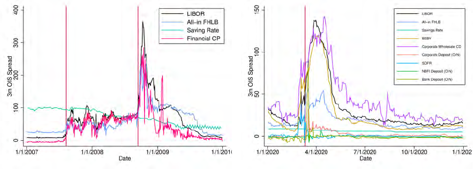
funding sources listed in Table 1 to LIBOR-OIS during periods of ﬁnancial distress. Figure 2 shows

data bearing on some key funding rates during the GFC in Panel (a) and during the COVID recession

in Panel (b). During the GFC, LIBOR-OIS started to increase around August 2007, at the collapse of

the asset-backed commercial paper (ABCP) market (Covitz, Liang, and Suarez, 2013). Between the

summer of 2007 and September 2008, LIBOR-OIS remained elevated and just below 100bp. Reported

LIBOR rates, however, were downward biased by manipulative reporting (Dufﬁe and Stein, 2015).

LIBOR-OIS returned toward normal levels near the end of the crisis.

Rates for retail deposits (proxied by savings and checking account rates from RateWatch) were

insensitive to movements in LIBOR-OIS spreads during the GFC. This is unsurprising. Most retail

deposits are insured and banks exhibit substantial market power over depositors, implying a low

sensitivity to changes in economic conditions (Driscoll and Judson, 2013; Drechsler, Savov, and

Schnabl, 2017). Rates on ﬁnancial CP, however, rose sharply with increases in LIBOR-OIS, as shown

in Figure 2. As documented by Ashcraft, Bech, and Frame (2010), rates on “safer" borrowing—such

as collateralized advances from FHLBs—were signiﬁcantly lower than LIBOR in the early stages of

the crisis, but rates on these somewhat lower-risk instruments also increased at the peak of the GFC.

(a) Global Financial Crisis (b) COVID-19 Recession

Figure 2:

Bank funding rates during ﬁnancial distress

. Various wholesale and deposit funding rates are

shown for periods covering the GFC (Panel (a)), and COVID pandemic (Panel (b)). Data Sources: FR2420, FRED, Bloomberg,

FDIC, RateWatch, FHLB Des Moines Historical Rate File. “All-in” FHLB spreads are calculated similarly to Ashcraft, Bech,

and Frame (2010), with additional parameters to capture equity cost for FHLB stock. Appendix A provides details. In the

COVID ﬁgure, Corporate Wholesale CD and Bank, Corporate, and NBFI O/N deposit rates are calculated from bank-level

transactions in the FR 2420 report. 3M CD rates reﬂect issuances with maturities between 89 and 92 days. "O/N" refers to

overnight rates. We aggregate trades by date, calculating the median daily interest rate weighted by transaction amount.

We exclude dates with fewer than 10 transactions, and carry forward the prior date’s rate. We then calculate a rolling

average rate that averages the interest rates paid on the ﬁve most recent trading dates, to smooth our series.

A similar pattern holds for the COVID recession, as shown in Panel (b) of Figure 2. LIBOR-OIS

increased throughout March, especially once the World Health Organization announced on March 11

that COVID-19 had become a global pandemic. However, LIBOR-OIS reached a much lower peak

than it had during the GFC.

For the COVID episode, we have more precise measures for bank funding costs. For instance,

we can obtain the rates for overnight corporate deposits and rates on deposits held by other banks

or non-bank ﬁnancial institutions (NBFIs). These rates, unlike retail deposit rates, are sensitive to

the effective fed funds rate. However, spreads of deposit rates over the effective federal funds rate

are relatively insensitive to LIBOR-OIS during the COVID episode.

We ﬁnd that an increase in

LIBOR-OIS of 100 basis points is associated with a mere 10-basis-point increase in overnight corporate

deposit spreads, a 5-basis-point increase in bank deposit spreads, and a 1-basis-point increase in

NBFI deposit spreads, as illustrated in Appendix Figure E.1.

As expected, wholesale bank funding spreads, such as spreads of corporate wholesale CDs

over OIS, closely track LIBOR-OIS during the COVID recession. A recently introduced Bloomberg

credit-sensitive three-month bank funding rate index, BSBY, also closely tracks LIBOR during the

COVID pandemic. In line with patterns observed during the GFC, “All-in” FHLB spreads also rose,

but peaked at less than 40% of LIBOR-OIS.

Our analysis of funding rate sensitivity shows that deposits are a cheap source of funding for

banks. While this is less surprising for retail deposits, it also holds for corporate deposits and for

open deposits from ﬁnancial institutions, which are sensitive to risk-free rates but not to LIBOR-

OIS. Wholesale funding is, in contrast, credit sensitive and more expensive. FHLB advances are

the cheapest form of wholesale funding while CDs and CP closely track LIBOR. Our analysis in

Section 5.1 shows that banks make little use of these more credit-sensitive forms of funding and,

to the extent they are used, the funding tends to be longer term and at ﬁxed rates. Our analysis,

however, does not preclude the use of unsecured wholesale funding—which is expensive for bank

shareholders especially during times of distress—to fund drawdowns. We next study the potential

need to fund drawdowns, using the funding sources discussed above.

5.3 Undrawn Commitments

Our theoretical analysis in Section 3 emphasizes that BHCs expose themselves to funding risk when

providing revolving credit. Table 2 shows that this risk is economically large. For the 20 largest

BHC, overall commitments sum to more than $3.5 trillion—more than twice the $1.6 trillion in

We construct these spread by averaging across overnight deposits held by either non-ﬁnancial corporates, banks or

NBFIs as reported in the FR 2420 and subtract the effective fed funds rate.

Table 2: Bank Credit by Loan Type for Large U.S BHCs as of December 31, 2019

Loan Type Util ($B) Comm ($B) % Utilized No. Banks

All Loans 1579.16 3551.52 44.46 21

Credit Line 543.76 1876.39 28.98 20

Term Loan 310.37 375.26 82.71 20

Other C&I 133.88 540.05 24.79 21

Commercial Real Estate 591.16 759.82 77.80 20

This table displays the distribution of utilized and committed credit across loan products. We source exposures from the

FR Y-14Q Schedule H1 B (corporate loans) and Schedule H2 (commercial real estate). Data are as of 2019q4. We include

only domestic C&I and CRE lending. US subsidiaries of foreign banks are excluded from our analysis. “Other” C&I

loans include non-revolving credit lines, capitalized lease obligations, standby letters of credit, other assets, fronting

exposures, commitments to commit, and exposures classiﬁed as “other.”

funded credit across C&I and CRE lending. The BHCs in our sample alone had around $1.3 trillion

of undrawn credit-line commitments, more than the total utilized credit from term lending and

revolving credit combined.

These unfunded commitments represent a substantial risk to bank liquidity if drawn during

times of stressed funding markets when bank credit spreads are elevated. Our theory suggests,

however, that linking lines to credit-sensitive reference rates has historically mitigated this funding

risk. Approximately 70% of these loans are indexed to LIBOR as of 2019 (Appendix Table E.4). Going

forward, this will not be the case. Our theoretical analysis implies that the funding risk associated

with credit lines may become much higher when LIBOR is replaced with a risk-free alternative such

as SOFR.

If borrowers draw on their lines in periods of distress, banks may need to pay expensive funding

costs in order to obtain the cash demanded by their borrowers.

As we show in Section 3, the

funding-spread component of these costs is borne by bank shareholders. However, as we have shown,

the manner in which banks fund these draws signiﬁcantly inﬂuences the funding spreads. We have

shown empirically that corporate deposit rates exhibit almost no credit sensitivity. Thus, the funding

cost to shareholders is minimal if borrowers leave most of their drawn funds on deposit at the same

bank. If, however, banks are forced to obtain funding at more credit-sensitive rates, shareholders can

bear a substantial cost.

For revolving credit lines, borrowers can draw and repay funds at their discretion, at least “on paper.” In practice,

however, not all commitments can be drawn, because covenants (Suﬁ, 2009) or other loan terms can limit the ability or the

incentives of borrowers to draw (Chodorow-Reich, Darmouni, Luck, and Plosser, 2021). Nonetheless, the extent to which

credit line draws need to be funded is largely out of a bank’s control.

5.4 Dynamics of Assets and Liabilities During Times of Distress

Given the large outstanding unfunded credit commitments of banks and the high associated potential

funding cost to bank shareholders, we next ask: How have bank balance sheets historically evolved

during periods of market stress accompanied by elevated bank funding spreads? Is the covariance

between drawdowns and bank funding spreads—a key determinant of credit supply according to

our theory in Section 3—positive and large? And how are drawdowns actually funded?

As descriptive evidence bearing on the evolution of bank balance sheets, Figure 3 shows cumu-

lative industry-level changes, in billions of dollars, of various balance sheet items in the periods

surrounding the COVID recession and the GFC. For the GFC, we rely on publicly available data

from the Federal Reserve H8 series, sourced via FRED. These data allow us to distinguish between

broad loan types (for example, C&I and home equity lines) on the asset side and, on the liability

side: deposits, interbank funding, and “other borrowing," which pools wholesale funding, FHLB

funding, and borrowing from the Federal Reserve. For the COVID recession, we use FR 2052a data,

which are more detailed. For instance, the FR 2052 gives us the ability to distinguish within the

categories of loans and deposits between counterparty types, allowing us to separate C&I lending to

large corporates and to small businesses. Figure 3 shows the dynamics of bank balance sheets, split

into assets and liabilities. Panels (a) and (b) show the dynamics for large US BHCs, which report

monthly in the FR2052a, around the COVID recession. Panels (c) and (d) show the dynamics for

large domestically chartered banks around the Lehman failure.

There is substantial growth in C&I lending following both shocks, partly or entirely driven by

credit line drawdowns, as shown in Panels (a) and (c) of Figure 3. During the COVID recession, we

observe for our sample of large banks that drawdowns on corporate credit lines increased by close to

$300 billion by April, which is an increase of almost 20% in total C&I lending (Li, Strahan, and Zhang,

2020; Acharya and Steffen, 2020). Most of these draws were from LIBOR-linked facilities

and were

driven by the largest ﬁrms (Greenwald, Krainer, and Paul, 2020; Chodorow-Reich, Darmouni, Luck,

and Plosser, 2021). Consistent with the presumption that ﬁrms drew on their lines to weather the

market turmoil, line draws were repaid quickly after the bond market started to recover (Darmouni

and Siani, 2022). Following Lehman’s failure, there was a $50 billion (6%) increase in C&I lending

overall, as large corporations drew on their lines in fear of future bank failures (Ivashina and

See Panel (a) of Figure E.3 in the Appendix.

(a) Loans During COVID Recession (b) Funding During COVID Recession

Figure 3:

Industry Assets & Liabilities in Periods of Distress.

This ﬁgure shows the evolution of aggregate

assets and liabilities during the GFC (following Lehman’s collapse) and during the COVID pandemic (following the

declaration of the global pandemic in March 2020). Values represent cumulative growth/decreases compared to the starting

month in billions of dollars. Data from the GFC are sourced from the FRED series for large domestically chartered banks,

adjusted for large M&A based on public notes to H8 series. Data from COVID are sourced from the FR 2052a monthly

balanced panel of 24 banks. Due to balance reclassiﬁcations between business segments in the FR 2052a, we exclude one

bank from our aggregate series for: small business loans, small business deposits. We include a version of the COVID

graphs for U.S. Branches of FBOs in Appendix Figure E.2.

Scharfstein, 2010).

Altogether, the increase in C&I lending due to drawdowns during both episodes

suggests that the covariance between drawdowns and bank funding spreads is indeed large.

We next turn to the evolution of bank liabilities, shown in Panels (b) and (d) of Figure 3. In

contrast to corporate lending, which increased during both periods, the evolution of bank liabilities

varied more between the COVID pandemic and the Lehman failure. Starting with the COVID

pandemic, we notice that the increase in bank liabilities was driven by debt whose pricing exhibited

limited credit sensitivity. Both corporate and ﬁnancial deposits increased by around $340 billion

(20%) in March 2020, almost entirely in open-maturity deposits (see Appendix Figure E.3). Rates

on these deposits largely tracked the federal funds rate during the COVID recession and were thus

far cheaper than unsecured wholesale funding (see Figure E.1). We also notice a striking increase

in FHLB advances—nearly $100 billion, or 40% of funding—in March 2020. The reliance on FHLB

advances in distress aligns with evidence from the GFC (Ashcraft, Bech, and Frame, 2010; Acharya

and Mora, 2015), as FHLBs provide cheaper funding than unsecured wholesale markets.

Retail deposits also rose signiﬁcantly in March of 2020, by $200 billion, with steady increases in

subsequent months. The increase in retail deposits can be explained in part by government stimulus

checks and precautionary savings (Cox, Ganong, Noel, Vavra, Wong, Farrell, Greig, and Deadman,

2020). Small business deposits also increased starting in April-May, likely related to the disbursement

of PPP funds. We also see a decrease in more expensive sources of short-term wholesale funding,

such as commercial paper (CP), certiﬁcates of deposits (CDs), and funding from off-balance sheet

conduits. The sole increase in expensive funding was in the form of long-term debt issuance, starting

in April-May 2020, which may have been a response to reduced yields that came on the back of the

Fed’s announcement on March 23 that it would purchase corporate bonds.

Following Lehman’s failure, we see an increase of around $160 billion (approximately 15%) in

“other borrowing”—a broad category of liabilities that includes short-term unsecured wholesale

funding, as well as advances from FHLBs. Deposits grew by over $300 billion (about 9%), of which

There was also a sustained increase in C&I lending after the ABCP run in 2007, partly due to draws on corporate credit

lines (Berrospide, Meisenzahl, and Sullivan, 2012). Further, there was limited growth in other loans after the COVID shock.

Following the March 2020 pandemic declaration, there was a decrease in aggregate retail lending. Small business only

increased in April with the launch of the Paycheck Protection Program (PPP) (Granja, Makridis, Yannelis, and Zwick, 2022).

After Lehman’s collapse, there were continued draws on home equity lines and consumer loans (and, possibly, credit

cards), although both increases generally followed pre-Lehman growth trends.

See Federal Reserve announces extensive new measures to support the economy, Board of Governors of the Federal

Reserve System, March 23, 2021 as well as Boyarchenko, Kovner, and Shachar (2022). Further, note that most of these

aggregate trends for the COVID pandemic also hold true in the cross-section of banks.

a signiﬁcant portion (by October 2008, nearly 50%) was in more expensive large time deposits. A

crucial difference between the GFC and the COVID recession is that the GFC saw a collapse of

interbank borrowing following Lehman’s failure (Afonso, Kovner, and Schoar, 2011), requiring some

banks to raise additional wholesale funds to make up for the lost interbank funding.

While both of these episodes saw signiﬁcant credit line drawdowns, the composition of aggregate

bank funding tilts toward more expensive sources during the GFC than during the COVID recession.

During the COVID recession, cheap deposit funding increased and relatively expensive wholesale

funding decreased. In contrast, the evidence suggests that the increase of deposit funding during

the GFC was in the form of relatively more expensive time deposits, especially at weaker banks

(Acharya and Mora, 2015). Further, corporate drawdowns during the GFC were akin to a run on

some banks (Ivashina and Scharfstein, 2010), forcing some banks to turn to relatively expensive

wholesale funding.

5.5 How Credit-Line Drawdowns Are Funded

We next address how banks ﬁnance drawdowns. At the bank level, we can exploit the granularity

of FR 2052a data and use cross-sectional variation to tighten our empirical understanding of how

drawdowns are funded during the COVID recession. At the borrower level, we use data from FR

Y-14Q, Compustat, and Capital IQ to study the relationships between drawdowns and cash holdings

during both the COVID recession and the GFC.

Bank-level Evidence.

We ﬁrst study the raw data and correlate changes in outstanding utilized

C&I exposure from the end of February 2020 through end of April 2020 with changes in corporate

deposits, FHLB advances, and unsecured wholesale funding. The left panel of Figure 4 shows linear

ﬁts. Here, for conﬁdentiality reasons, we group BHCs into bins, with several BHCs per bin.

There is a strong correlation between an increase in C&I loans on the one hand and corporate

deposits and FHLB advances on the other, with the slope being much higher for the former. Thus,

our ﬁndings suggest that drawdowns in March and April 2020 were by and large for precautionary

purposes, with corporates drawing their credit lines but leaving the drawn amounts in their deposit

accounts. Firms plausibly chose to draw the cash on their lines before lenders might have invoked

covenants that could have blocked them from doing so at a later stage. Further, to the extent that this

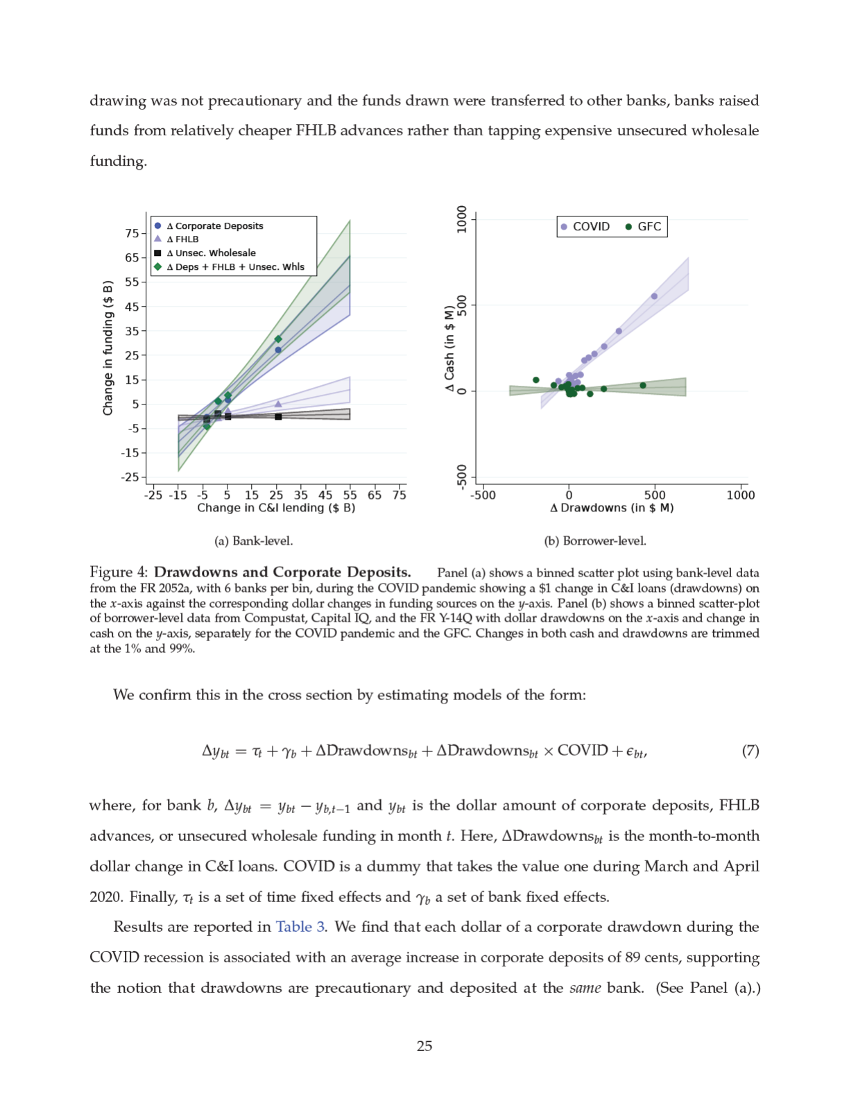
However, this was mostly driven by the largest banks in our sample. For the regional banks in our

sample, captured in in Panel (b), only around 40% of drawdowns were deposited. The regional

banks instead relied on advances from FHLBs, which funded around 40% of additional draws.

Importantly, the banks in our sample did not require additional unsecured wholesale funding to fund

corporate draws, irrespective of their business model. In fact, the largest banks experienced deposit

growth signiﬁcantly in excess of their drawdowns, as shown in column (5) of Panel (a).

This was

driven by a growth in deposits at non-bank ﬁnancial institutions, possibly because of Federal Reserve

asset purchases and the concentration of reserve balances at larger banks. The simultaneous increase

in deposits and drawdowns is also consistent with the theoretical synergies of banks as liquidity

providers through both deposits and committed credit lines (Kashyap, Rajan, and Stein, 2002).

Borrower-level Evidence.

Our ﬁndings thus far indicate that, during the COVID shock, a

substantial portion of drawdowns were deposited. However, our bank-level data do not include

account-level deposit information, so we cannot establish a direct link between drawdowns and

precautionary deposit increases at the borrower level. To address this concern, we turn to granular

borrower-level information from the FR Y-14Q, Compustat, and Capital IQ to examine the extent

to which draws were associated with an increase in borrower cash—a proxy for corporate deposit

holdings. We conduct this analysis for both COVID and the GFC to see how drawdown motives

differed across the two stress events.

The right panel of Figure 4 shows the correlation between changes in borrower-level drawdowns

and changes in cash holdings for both the GFC and COVID recession. The data indicate a strong

correlation for the COVID recession, in line with precautionary drawdown motives. This correlation

is not present during the GFC, in line with ﬁrms not depositing drawdowns in the banking sector

during this episode.

A potential explanation for the fact that regional banks had to raise relatively more funding from FHLBs is that

drawdowns on syndicated facilities may not be deposited at the lending bank but rather at the main relationship bank of

the borrower. See also Kiernan, Yankov, and Zikes (2021) for an analysis of liquidity co-insurance in syndicates. While we

do not observe each borrower’s relationship bank, there is a signiﬁcant correlation between bank size and being agent

on a syndicated facility (which is possibly correlated with being the main relationship bank. Our results also echo the

ﬁndings of Glancy, Gross, and Ionescu (2020), that smaller banks saw a smaller portion of drawdowns deposited than did

larger banks. However, we show that even among the largest US banks (those with over $ 100 billion in assets), there were

differences in the fractions of deposited line draws.

This increase in both total deposits and drawdowns during COVID is also consistent with a “ﬂight to safety” during

previous stress events (Gatev and Strahan, 2006), excluding the GFC when banks were at the center of the crisis (Acharya

and Mora, 2015).

Table 3: Drawdowns and Deposits in the Cross-Section: Monthly Data.

Dependent variable ∆ Corp. ∆ FHLB ∆ Unsec. ∆ Total ∆ Total

Deposits WSF Cols. (1-3) Deposits

Panel A: All Banks

(1) (2) (3) (4) (5)

∆ Drawdowns 0.01 -0.01 -0.00 0.00 -0.03

(0.01) (0.03) (0.01) (0.03) (0.03)

∆ Drawdowns × COVID 0.89*** 0.16 0.02 1.07*** 1.79**

(0.27) (0.10) (0.05) (0.37) (0.78)

N 1107 1107 1107 1107 1107

No. Banks 25 25 25 25 25

0.397 0.177 0.100 0.394 0.424

Panel B: Regional Banks Only

(1) (2) (3) (4) (5)

∆ Drawdowns 0.01* -0.01 -0.00 -0.01 0.02

(0.00) (0.03) (0.01) (0.03) (0.02)

∆ Drawdowns × COVID 0.42** 0.40*** -0.05 0.77*** 0.37

(0.20) (0.14) (0.06) (0.23) (0.46)

N 522 522 522 522 522

No. Banks 12 12 12 12 12

0.387 0.320 0.143 0.381 0.454

Notes: This table reports estimates from a bank-month-level panel regression of the form:

∆y

= α + ∆Drawdowns

+ ∆Drawdowns

× COVID + γ

+ η

+ e

Robust standard errors in parentheses; *, **, and *** indicate signiﬁcance at the 10%, 5%, and 1% level, respectively. We

exclude from our analysis the bank-month in which BB&T merged with SunTrust. We include bank and time ﬁxed effects

in all speciﬁcations. The dependent variable in column (3), unsecured wholesale funding (WSF), captures short-term

wholesale funding categories: CP, CD, non-prime brokerage free credits, and other unsecured wholesale funding. The

dependent variable in column (4) is the change in the sum of corporate deposits, FHLB advances, and unsecured wholesale

funding. Data Source: FR2052a.

We next estimate cross-sectional regressions of the form:

∆Cash

= α + β

∆Drawdowns

+ X

+ e

, (8)

where

∆Cash

is the change in the dollar amount of deposit holdings

of borrower

and

∆Drawdowns

is the change in the dollar-amount of drawdowns over the same time period.

Results can be found in Table 4. The estimation conﬁrms the patterns from the right panel of

Figure 4. We ﬁnd that for this period, a one dollar increase in drawdowns is associated with an

increase in cash holdings of 86 to 97 cents, roughly in line with our bank-level evidence reported

earlier. In contrast, for the GFC, we ﬁnd no statistically signiﬁcant relationship between drawdowns

For our analyses using Compustat, we use CHQ to measure cash. Importantly, cash does not include money market

fund holdings or reverse repo transactions. For our analyses solely using the FR Y-14Q in columns 1 and 2 of Table 4, since

the FR Y-14Q does not separate cash from cash equivalents, these analyses pool both cash and cash-like instruments.

Table 4: Precautionary Draws: COVID versus GFC

COVID GFC

Y-14 Y-14 / Compustat

(1) (2) (3) (4) (5) (6) (7)

∆ Util. 0.97*** 0.97*** 0.92*** 0.86*** -0.01 0.04 -0.01

(0.07) (0.07) (0.11) (0.09) (0.07) (0.07) (0.07)

Industry FE Yes Yes Yes Yes Yes Yes Yes

Fiscal Year No Yes No Yes No Yes Yes

Match Quality No No No No Yes

Data Y-14 Y-14 / Compustat Compustat/CIQ

.275 .275 .314 .303 .0791 .0859 .148

N 7130 7130 1635 1468 1317 1217 811

Notes: This table shows estimates from cross-sectional regressions of the form

∆Cash

= α + β

∆Drawdowns.

+ X

+ e

where the dependent variable is the change in cash for ﬁrm

before and after the shock,

∆Drawdowns

is the change in

credit-line utilization of ﬁrm

, and

are ﬁrm controls, such as industry ﬁxed effects and other cash ﬂows. Columns

1-2 use quarterly data from the FR Y-14Q (aggregated by borrower TIN) of borrowers who reported ﬁnancials in either

2019q3 or 2019q4 and also in March 2020. Columns 3-4 merge Y-14 credit line usage to updated ﬁnancials as reported in

Compustat. Columns 5-7 conduct ﬁrm level analyses on annual data during the GFC using drawdowns from Capital IQ

and ﬁnancials from Compustat. In Columns 2, 4, 6, and 7, we restrict to borrowers whose ﬁnancial statement “as-of” dates

correspond to calendar year quarters (that is, March, not February). In Column 7, we restrict our sample to a sub-sample

of ﬁrms where we match long-term debt between Compustat and Capital IQ within 10% on average. We trim both

∆

cash

and

∆

draws at the 1% and 99% levels to attenuate the impact of outliers. Robust standard errors in parentheses; *, **, and

*** indicate signiﬁcance at the 10%, 5%, and 1% levels, respectively.

and deposits (columns 5-7).

This indicates that drawdowns were not deposited in the banking

system, but instead were deployed elsewhere – either via other investments or for ﬁrm expenditures,

such as investment or compensation. Importantly, since these drawdowns were apparently not

merely left in deposit accounts,

banks would have been required to fund them via other methods,

which may have included costly unsecured wholesale funding.

6 Calibrated Impacts of Reference Rates on Credit Supply

In this section, we quantify how the choice of loan reference rate affects the equilibrium provision of

revolving credit by large US banks. To do this, we parameterize and calibrate versions of the simple

theoretical model presented in Section 3, based on the empirical analysis and insights of Section 5.

This is consistent with evidence from Ivashina and Scharfstein (2010) that drawdowns following Lehman’s failure were

of the form of a bank run on institutions with greater Lehman exposure. It is also in line with results from Berrospide

and Meisenzahl (2021) that drawdowns during the GFC were not precautionary in nature and instead funded capital

expenditures.

For drawdowns to be precautionary, it is necessary for deposit holdings to increase in response to credit-line drawdowns.

Since we do not observe an increase in deposit holdings following drawdowns, we can conclude that drawdowns following

Lehman’s failure were not precautionary. This does not preclude reshufﬂing of corporate deposits among banks; however,

that poses a different funding risk beyond the scope of this paper.

We consider the implications for credit provision of heterogeneous banks and borrowers. Further, we

analyze how ex-ante credit supply depends on the extent to which line draws are expected to be left

on deposit at times of high bank funding stress. Finally, we show how the welfare-maximizing degree

of credit sensitivity of a reference rate depends on the quality of the bank or the banking system.

Consistent with the insights gained from our theoretical model, welfare-maximal reference rates are

more credit sensitive for banking systems of lower credit quality, given their greater debt-overhang

costs for funding line draws during crisis periods.

Parametrization and Outcomes.

We start by parameterizing a version 75 of the model discussed

in Section 3. The probability density of the spread

between LIBOR and OIS is modeled as a

mixture of normals, as plotted in the left side of Figure 5. In our baseline model, with probability

0.96,

log W

has a mean and variance ﬁt by maximum likelihood to daily LIBOR-OIS observations

from January 2005 to April 2021. With a “crisis” probability of 0.04, however,

has a log-normal

distribution with a mean of 350 basis points, which is roughly the highest level reached by LIBOR-OIS

during the GFC, and with a standard deviation of 40 basis points. Because our model has annual

periods,

this corresponds to the assumption that a GFC-like event is expected to occur once every

quarter century. We later quantify the sensitivity of our results to varying the likelihood of this crisis

shock, among other key parameters.

Our representative bank is assumed to be of “LIBOR quality,” thus having an unsecured wholesale

credit spread of

. Later, we consider the implications of the model for banks with wholesale funding

costs that are higher or lower than LIBOR. The bank has a continuum of borrowers of total mass

A borrower’s cash liquidity beneﬁt is speciﬁed as

b(q, ψ) =

1−α

1 − α

, (9)

for a positive constant

, where

is the borrower’s liquidity preference shock.

The price elasticity

of drawn credit is 1

/α

at any line utilization strictly between 0 and 1. We take a baseline assumption

α =

25, implying an elasticity of 25 that is in the range suggested by prior empirical work (for

Because we calibrate to quarterly LIBOR-OIS and our model has a single annual period of drawing, we are effectively

assuming that drawn loans are rolled over quarterly for one year.

This speciﬁcation respects the natural restriction that, in equilibrium, the marginal value

(Q(L)

ψ)

of drawn funds is

at least 1 in every state.

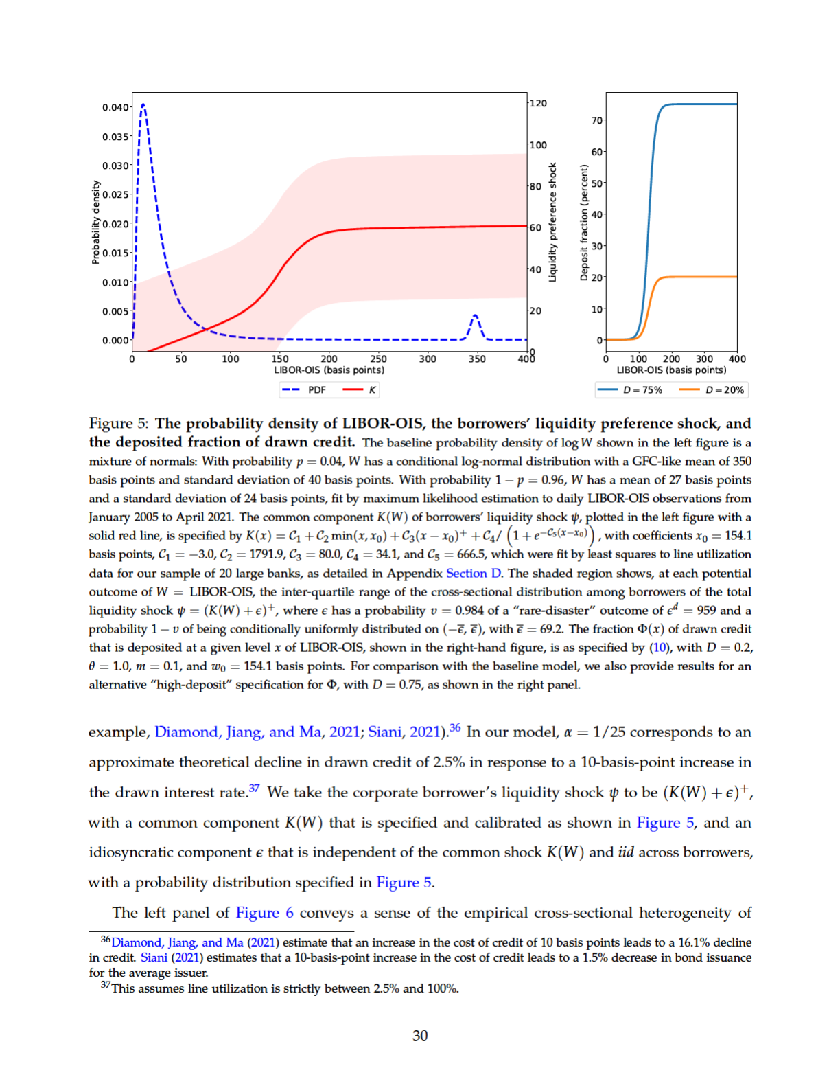
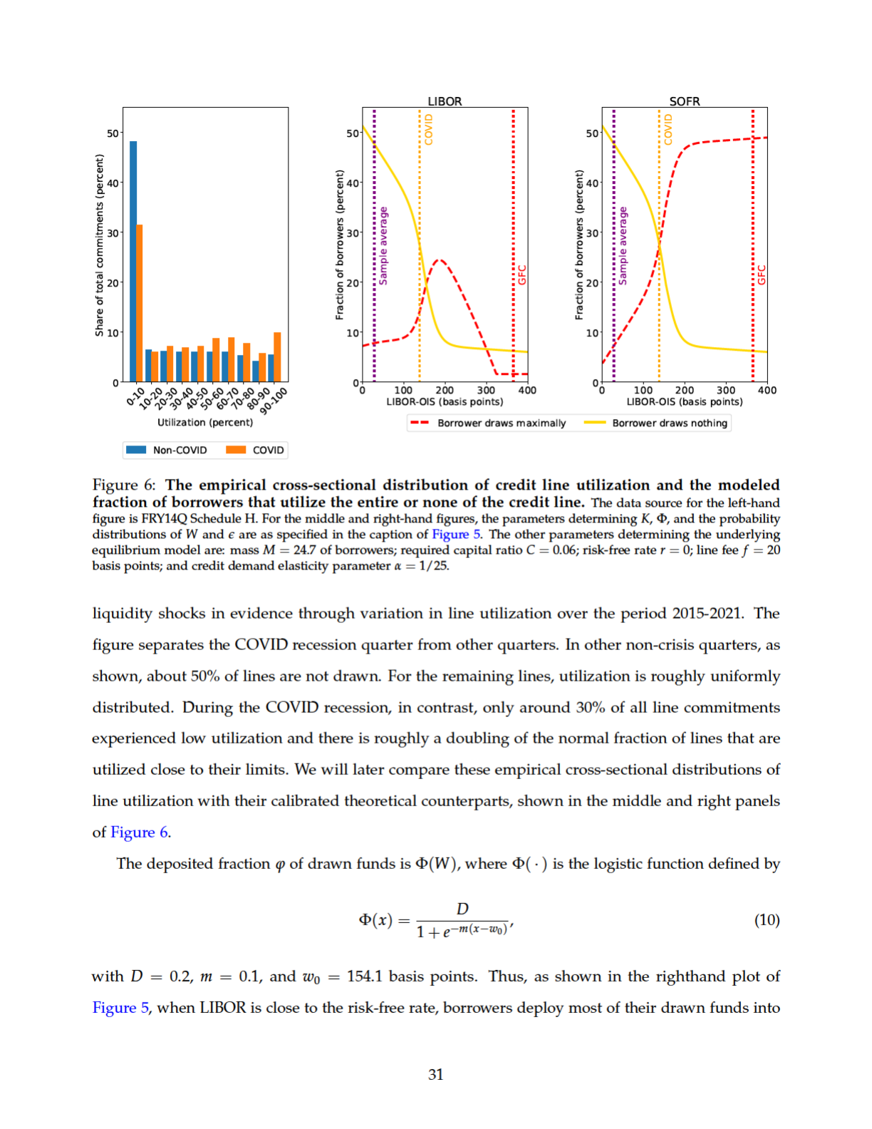
business operations and leave very little on deposit. However, in crisis states, when LIBOR-OIS is

large, borrowers could potentially deposit a higher fraction of drawn funds, given the precautionary

motives that may apply in a macro shock like COVID, as documented in Section 5.5. The deposited

fraction Φ(x) of drawn funds that it increases with x to a “crisis limit” of D.

Section 5.5 shows that even when LIBOR-OIS rose to over 300 basis points during the GFC, there

was little depositing of drawn funds. What matters for credit line provision is the ex-ante expected

fraction of drawdowns left on deposit, conditional on LIBOR-OIS. Future shocks to LIBOR-OIS could

result in low depositing of drawn funds, as with GFC, or much higher depositing behavior, as with

COVID. Our base-case choice of

D =

0.2 is plausibly between the average GFC and COVID outcomes,

but represents an assumption rather than an empirically identiﬁed parameter. Given the crucial

role of this parameter, we will analyze the effect of varying

. We will also run experiments that

vary

jointly with the bank’s expected unsecured wholesale funding costs, given the observed

heterogeneity of depositing behavior across bank types that we uncovered in Section 5.5.

From Section 3, the modeled optimal quantity of credit drawn from a line of size

with a ﬁxed

spread s over the chosen reference rate R is

Q(L) = min



(K(W) + e)

(1 + R + s)

−1/α

, L



. (11)

For states in which the borrower is drawing more than zero and less than the line limit

, the optimal

drawn amount

Q(L)

is strictly decreasing in the drawn interest rate

R + s

and strictly increasing in

both the macro liquidity shock K(W) and the idiosyncratic liquidity shock e.

The calculations in Section 3 determine, for any candidate reference rate

, the bank’s menu

{(L

s(L)) : L ≥

}

of offers of line size

and ﬁxed interest rate spread

s(L)

over the reference rate.

In equilibrium, borrowers pick their optimal line size

from this menu. The exact law of large

numbers implies that the aggregate amount of drawn credit is

M · E[Q(L) | W] = M · E



min



(K(W) + e)

(1 + R + s)

−1/α

, L







. (12)

This equality holds with probability equal to one under measure-theoretic conditions on the space of borrowers

and states of the world described by Sun (2006). The fraction of borrowers whose idiosyncratic liquidity shocks have

an outcome in any given interval

is the same as

P(e ∈ (a

b))

. This implies

(12)

and

(13)

, by integration over the

probability distribution of e.

Similarly, the fraction of borrowers that draw their lines to the limit is

P[Q(L) = L | W] = P



(K(W) + e)

(1 + R + s)

−1/α

≥ L





. (13)

For simplicity, we take the risk-free rate

to be zero and the loss given default (LGD) on the bank’s

unsecured funding to be 50%. The proportional line fee

is assumed to be 20 basis points. The

parameters determining the macro component

K(W)

and idiosyncratic component

of the borrowers’

liquidity preference shocks, and the quantity

of borrowers, are jointly ﬁt to our data bearing on

the aggregate quantity of credit lines and the variation across borrowers and states of credit-line

utilization, for our sample of historical experience for LIBOR-linked credit lines, for which the

reference rate is

R = r + W

. Appendix D provides details on the ﬁtting method. As Figure 5 shows,

is an increasing function, implying that the cross-sectional average of line utilization increases

with bank funding costs. Aside from parameters chosen to match speciﬁc empirical counterparts,

the parameters are chosen to minimize the weighted sum of squares of (i) the difference between

the empirical average of the total dollar quantity of lines and its model-implied analogue

M · L

, (ii)

for each quarter, the difference between the actual quantity of line draws and the model-implied

quantity of line draws given by

(12)

, and (iii) for each quarter, the difference between the actual

fraction of lines drawn to their limits and the model-implied analogue given by (13).

With the resulting parameters calibrated to our sample of historical experience for LIBOR-linked

credit lines, we next consider the effects of varying the chosen reference rate, bank quality, borrower

deposit behavior, and other properties of the model.

The Effects of LIBOR-SOFR Transition on Credit Supply.

The model-implied impact of a

transition from LIBOR to SOFR on credit provision through revolvers by large US banks is shown in

Figure 7. This ﬁgure displays, for each outcome of LIBOR-OIS, the equilibrium interest rate paid per

unit of credit drawn (left panel) and the aggregate amount of line commitments and drawn credit

(right panel). For the representative calibrated bank, transition from LIBOR to risk-free reference rates

causes a modest reduction of about 5% in equilibrium line sizes and a reduction of around 3% in the

expected quantity of drawn credit, but with a substantial change in line utilization across different

outcomes for LIBOR-OIS. For example, with SOFR as a reference rate, our baseline calibration implies

Based on an informal communication, we observed that a large non-bank borrower had line fees for its two revolvers

of 15 basis points and 25 basis points.

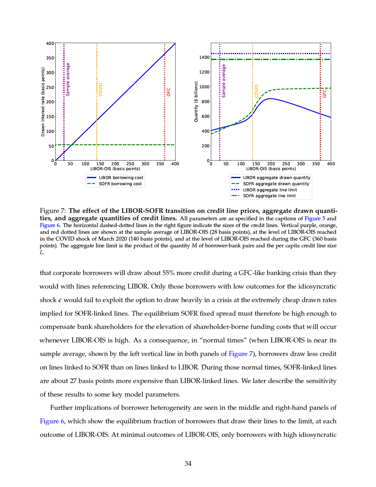
liquidity shocks exhaust their line limits. However, as LIBOR-OIS increases, the associated increase

in the drawn rate on LIBOR-linked lines eventually dominates the liquidity preference shocks of

most borrowers, and LIBOR lines are relatively less likely to be drawn than SOFR lines. By contrast,

when LIBOR-OIS is high, the low drawn interest rate on SOFR-linked causes most borrowers to draw

SOFR lines to the limit.

Our model is calibrated, in part, to approximate the empirical fraction of borrowers that draw

their lines to the maximum in normal times. The left panel of Figure 6 shows that, empirically,

around 5.5% of borrowers were at or close to their line limits in normal quarters, and that this fraction

doubles to around 9.9% during the COVID recession. In our calibrated model, as shown by the

middle panel of the ﬁgure, around 8% of borrowers are at their line limits during normal times, and

this modeled fraction increases to around 14% during the COVID recession. For SOFR-linked lines,

in contrast, while around 7% of borrowers draw the maximum amount during normal times, around

27% of borrowers would have been at the line limit during the COVID recession and a striking 49%

of borrowers are predicted by the model to be drawing revolvers to their limits if LIBOR-OIS reaches

its GFC level.

Model sensitivity.

Table 5 shows a sensitivity analysis of some of the main results with respect

to two key parameters: the price elasticity 1

/α

of borrower demand for credit and the probability

of a GFC-like increase in LIBOR-OIS. For example, reducing the assumed price elasticity of credit

demand from 25 to 24 (by 4%) causes the model-implied impact of LIBOR-to-SOFR reference-rate

transition on the aggregate dollar amount of lines to change from a 5.5% reduction in lines at

baseline to a 7.5% reduction in lines, after re-calibrating other parameters for best ﬁt following the

procedure described in Appendix D. Because of the resulting adjustment of other parameters, this is

a check on model robustness, and not a comparative-static analysis of the effect of price elasticity

on credit demand. Increasing the likelihood of a GFC shock from 4% at baseline to 5% leads to an

increase in the model-implied reduction in aggregate lines from 5.5% to 8.1%. A higher probability

of distressed funding markets implies relatively higher expected debt-overhang costs to banks for

offering SOFR lines. Overall, it is important to caveat that, while our ﬁndings are qualitatively robust,

the magnitudes of transition impacts are uncertain due to model sensitivity.

Table 5: Sensitivity of modeled transition impacts to demand elasticity and crisis probability

Total credit lines ($ billions) Impact on drawn rate (bps) Impact on drawn credit

(1) (2) (3) (4) (5) (6) (7)

Assumed parameters LIBOR- SOFR- Impact LIBOR-OIS LIBOR-OIS LIBOR-OIS LIBOR-OIS

linked linked at 28 bps at GFC level at 28 bps at GFC level

1/α = 25, p = 4% 1,444 1,365 −5.5% 22.3 −313.7 −5.43% 67.6%

1/α = 24, p = 4% 1,602 1,483 −7.5% 28.9 −307.1 − 6.80% 53.2%

1/α = 25, p = 5% 1,538 1,412 −8.1% 30.7 −305.3 −7.50% 60.9%

Notes: Row 1 of the table corresponds to the baseline model, which assumes an unconstrained price elasticity of credit

demand of 25 (

α =

0.04) and assumes a probability of

p =

4% for a GFC-like conditional distribution of LIBOR-OIS. Row 2

corresponds to the model that is re-calibrated to empirical data based on an assumed price elasticity of 24 (

α =

0.04167)

and

p =

4%. Row 3 corresponds to the model that is re-calibrated to empirical data based on an assumed price elasticity of

25 and

p =

5%. Column 1 is the modeled aggregate quantity of credit lines if LIBOR is the reference rate. Column 2 is

the aggregate quantity of credit lines if SOFR is the reference rate. Column 3 is the percentage difference between the

quantities of SOFR-linked lines and LIBOR-linked lines. Column 4 is the difference between the drawn interest rates on

SOFR-linked lines and LIBOR-linked lines when LIBOR-OIS is at its sample average of 28 basis points. Column 5 is the

difference between the drawn interest rates on SOFR-linked lines and LIBOR-linked lines when LIBOR-OIS is at the GFC

level of 360 basis points. Column 6 is the percentage difference in the drawn amounts of credit on SOFR-linked lines and

LIBOR-linked lines when LIBOR-OIS is at its sample average of 28 basis points. Column 7 is the percentage difference in

the drawn amounts of credit on SOFR-linked lines and LIBOR-linked lines when LIBOR-OIS is at the GFC level of 360

basis points.

Bank Heterogeneity.

Section 5 provides evidence of substantial heterogeneity across banks in

how drawdowns are funded during the COVID recession. We ﬁnd that while banks, on average,

received 90 cents of corporate deposits for each dollar drawn, some banks receive much higher

deposit inﬂows than others. For instance, we ﬁnd that regional banks (listed in Appendix Table A.1)

received only about 40 cents in deposits per dollar drawn and had to raise the remaining funds with

more expensive wholesale funding such as FHLB advances. There is also substantial heterogeneity

across large banks in unsecured funding spreads (Berndt, Dufﬁe, and Zhu, 2021). We therefore turn

next to an analysis of how the implications of reference rate transition for credit provision vary with

the type of bank.

We ﬁrst consider the effect of varying bank funding costs by taking the external funding spread

of the modeled bank to be

S = θW

, for some constant

that we allow to vary parametrically.

For

our base-case calibration, we took

θ =

1, corresponding to a LIBOR-quality bank. For instance, with

θ =

1.5, the credit spread of the modeled bank is 50% higher than that of an average LIBOR-quality

bank, state by state. The left panel of Figure 8 illustrates how the equilibrium dollar quantity of

From the results of Section 3, for a given θ, the contractual spread s(L) over LIBOR, with an LGD of 50%, is

s(L) =

E[2θWQ(L)(1 − δ(1 + R − (1 + C)(1 − Φ(W))θW))]

E[δ2θWQ(L)]

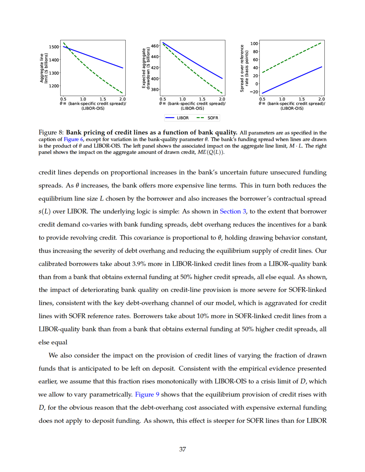
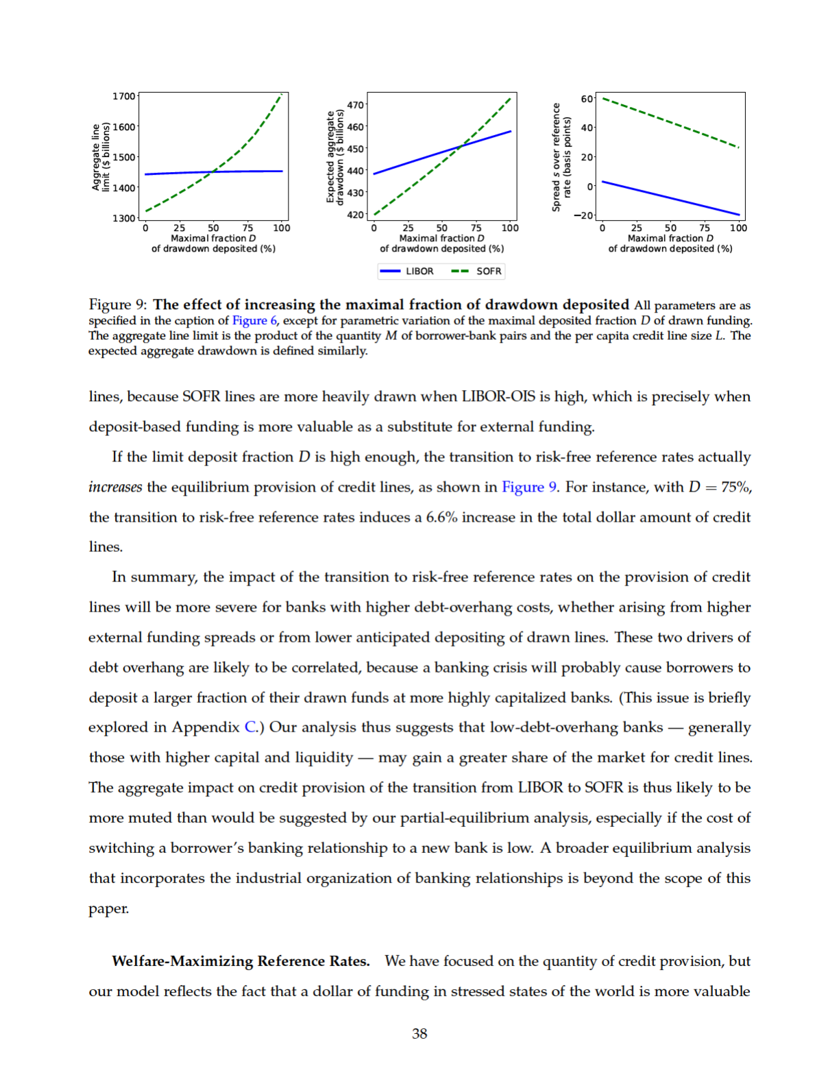
to borrowers than a dollar of funding in normal states. One can view a credit line as a form of

insurance against liquidity shocks. Thus, the welfare-maximal reference rate could in principle be

quite different than the reference rate that maximizes the expected quantity of credit granted. We

now consider the welfare-maximizing degree of credit sensitivity of the reference rate, taking as our

welfare measure the expected liquidity beneﬁt to borrowers, which is

E[b(Q(L)

ψ)]

. All other costs

and beneﬁts in our model are merely transfers. Figure 10 shows how total welfare in our model

depends on the degree

of credit sensitivity of the reference rate. The risk-free reference rate, SOFR,

corresponds to

λ =

0. LIBOR corresponds to

λ =

1. A point

on the horizontal axis corresponds to

a reference rate that is the linear combination λ × LIBOR + (1 − λ)× SOFR.

The vertical dotted line in the left-hand ﬁgure indicates the convex combination of LIBOR and

SOFR deﬁning the reference rate that maximizes the welfare gain of a new credit line. As shown,

our analysis suggests that the welfare-optimal reference rate for our modeled LIBOR-quality bank

has about 80% of the credit sensitivity of LIBOR. The right-hand panel of the ﬁgure shows that the

reference rate that maximizes the provision of credit lines is slightly more credit sensitive.

Our marginal analysis of credit-line provision, however, ignores the impact of reference-rate

design on bank distress costs. Because there can be non-zero bank distress costs associated with

heavier drawing of lines in stressed states, our marginal analysis understates the credit sensitivity of

welfare-optimal reference rates that would apply in a full general-equilibrium setting.

The welfare-maximizing reference rate varies with the type of bank or banking system. Figure 10

corresponds to our base case of a LIBOR-quality bank (

θ =

)

and a maximal anticipated deposited

fraction

D =

0.2 of drawn funds. Figure 11 shows how welfare is affected by the credit sensitivity

of the reference rate for a “low-debt-overhang bank,” whose credit spread is only

θ =

75% of

LIBOR-OIS, and for a “high-debt-overhang bank," whose credit spread is assumed to be 50% higher

than LIBOR-OIS. Whereas the low-debt-overhang bank is assumed to receive in deposits a maximum

D =

75% of drawn funds, the high-debt-overhang bank is assumed to receive a maximum of only

D =

20% in deposits. A negative relationship between bank funding spreads and the fraction of

deposited line draws is natural, as we discuss in Appendix C.

Figure 11 shows that the welfare associated with credit-line provision by high-debt-overhang

banks is maximized by a reference rate whose credit sensitivity is close to that of LIBOR. Low-

debt-overhang banks, however, offer better credit provision, in the sense of this experiment, with a

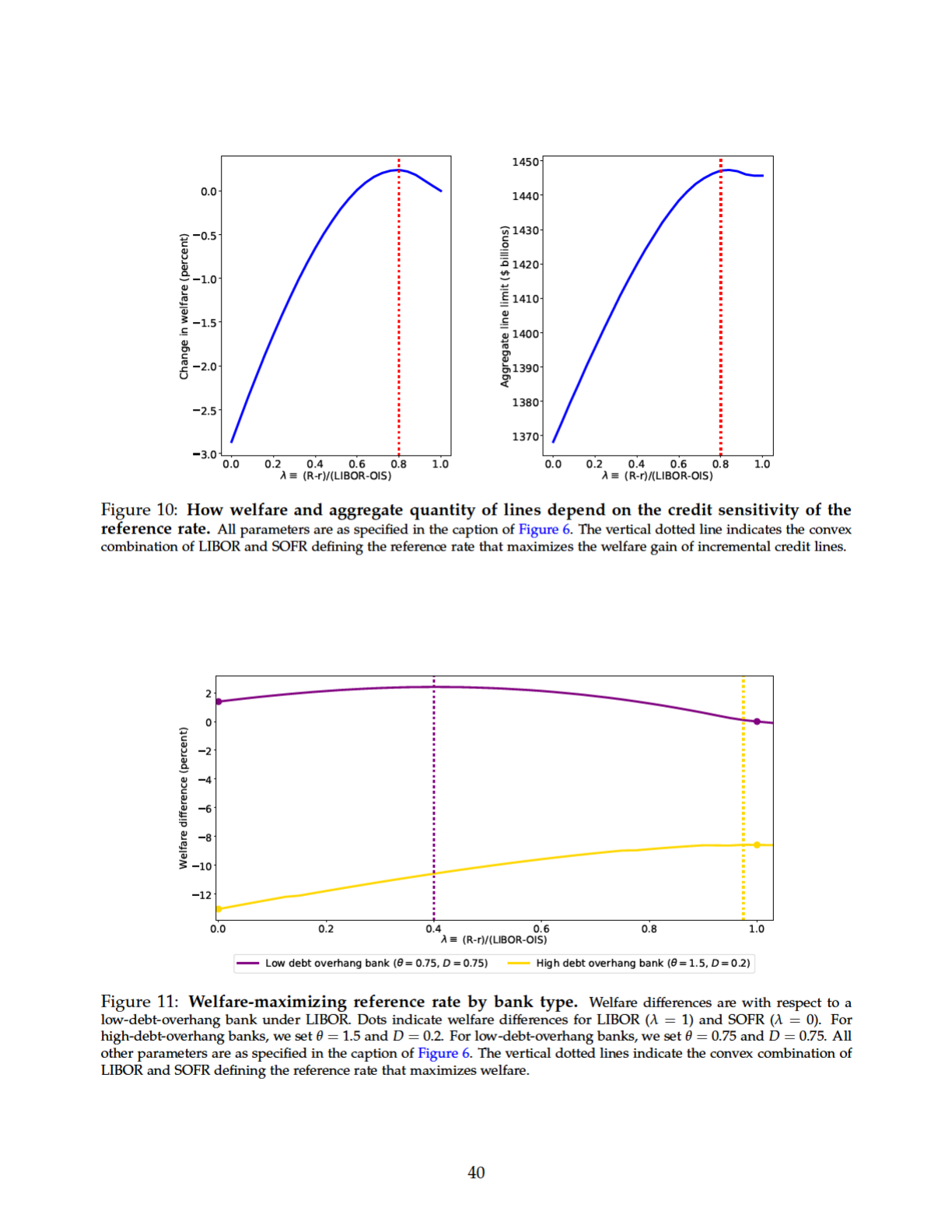
reference rate that is closer to the risk-free rate, although the responsiveness of welfare to the credit

sensitivity of the reference rate is muted for low-debt-overhang banks.

This analysis may help explain why regional US banks have dominated the collection of banks

arguing that the transition to risk-free reference exacerbates bank funding shocks and reduces

incentives for credit provision. Their joint letter to the heads of the US banking authorities

emphasized that “borrowers may ﬁnd the availability of low cost credit in the form of SOFR-linked

credit lines committed prior to the market stress very attractive and borrowers may draw-down those

lines to ‘hoard’ liquidity. The natural consequence of these forces will either be a reduction in the

willingness of lenders to provide credit in a SOFR-only environment, particularly during periods of

economic stress, and/or an increase in credit pricing through the cycle.” Our analysis in Appendix B

shows that the wholesale unsecured funding spreads of regional banks are only slightly higher than

those of the largest US bank holding companies,

an estimated average of 22 basis points higher

post-GFC, and about 10 basis points higher from 2015-2021, controlling for maturity and time ﬁxed

effects. That reference-rate transition may have a higher impact on the provision of revolvers by

regional banks is also suggested by our ﬁnding in Section 5 that regional banks experienced a much

lower extent of depositing of drawn lines during the Covid shock of 2020 than did the largest banks

in our sample.

7 Discussion

Bank shareholders do not break even when banks raise cash to invest in assets unless the bank

extracts a proﬁt margin from its counterparties that offsets the credit-spread component of the bank’s

funding cost. In market practice, this wedge is called a “funding value adjustment” (Andersen,

Dufﬁe, and Song, 2019). We ﬁnd that the transition from credit-sensitive reference rates like LIBOR

and EURIBOR to risk-free reference rates such as SOFR and ESTR increases this wedge by inciting

borrowers to draw on their lines even more heavily during periods of market stress. This is so

See the letter of September 23, 2019 from Credit Sensitivity Group to Randall Quarles, vice-chair of supervision of the

Board of Governors of the Federal Reserve System, Joseph Otting, Comptroller of the Currency, and Jelena McWilliams,

chair of the Federal Deposit Insurance Corporation.

These estimates arises from ﬁtting the model

= β

+ β

+ δ

+ e

, where

is the average secondary-

market yield spread of debt instrument

during month

is its remaining maturity,

is an indicator for regional

banks (1 if regional, 0 otherwise),

is a month ﬁxed effect, and

is a noise term. We ﬁt by weighted least squares, with

weights proportional to traded volumes, corresponding to best linear unbiased estimation under the assumption that the

model is correctly speciﬁed with noise terms that are uncorrelated and have variances proportional to the reciprocals of

trade volumes.

because drawing on a line referencing a risk-free rate is typically very cheap when credit markets are

stressed. When a SOFR-linked line is originally contracted, the higher expected future funding cost

wedge is priced into the terms of credit facilities, leading to an equilibrium reduction in revolving

credit for our representative calibrated bank. We show that this impact on credit provision is smaller

for banks with lower funding spreads, or even reversed if it is anticipated that borrowers will leave

the majority of their future line draws on deposit at the same bank. Empirically, we ﬁnd that the

extent to which line draws induced by the COVID pandemic shock were left on deposit was much

lower at regional US banks than at the largest US banks. Because of this, reference rate transition

is likely to impact the provision of credit lines more for regional US banks than for the largest US

banks.

As opposed to prior work offering a risk-sharing rationale for credit-sensitive reference rates, our

ﬁnding that credit-sensitive reference rates improve credit provision is not driven by hedging or risk

aversion, and does not apply to term loans, which do not give borrowers the option to increase the

loan size when market stress increases.

Our paper also identiﬁes a new channel of synergy between deposit taking and credit-line

provision. Kashyap, Rajan, and Stein (2002) emphasize the synergy associated with a bank’s ability to

draw on a common pool of liquid assets, whether to meet line draws or for other funding needs. We

show that there is a complementary source of synergy between these two business lines – revolvers

and deposit taking – via a reduction in debt-overhang costs to bank shareholders. This synergy is

stronger for risk-free reference rates than for credit-sensitive reference rates because, when markets

are stressed and bank funding costs rise, borrowers are expected to draw more heavily on lines

linked to risk-free reference rates, making the inﬂow of cheap deposits especially valuable.

The synergy between revolvers and deposit taking is arguably weaker for syndicated loans,

because the associated deposit inﬂows tend to be more concentrated among the syndicate of banks,

especially at the lead arranger. Given that deposit inﬂows are relatively more valuable under risk-free

reference rates, we speculate that the transition away from credit-sensitive rates may create incentives

to change loan pricing terms across a syndicate or even lead to a reduction in loan syndication.

Our results also suggest that reference-rate transition may cause some credit-line provision to

move away from banks with high funding costs toward banks with lower funding costs. A key metric

here is the blended average spread on marginal sources of funding of credit-line draws, which is a

combination of the spreads on wholesale external funding and on corporate deposits, to the extent

that line draws are left on deposit. However, relationships between banks and corporate borrowers

are somewhat sticky; otherwise credit lines would already have been highly concentrated at banks

with the lowest funding costs, well before LIBOR transition. This is clearly not the case. Corporate

borrowers are paired with banks in somewhat stable relationships, whether because of monitoring

costs, geography, or other reasons (Chodorow-Reich, 2013; Schwert, 2018). It is beyond the scope of

our work to analyze the degree to which the stability of banking relationships could be disrupted by

reference-rate transition.

Adverse impacts of reference-rate transition on credit-line provision could seemingly be mitigated

by the ability of borrowers to substitute some of their credit lines with term loans, given the negligible

impact of reference rate transition on the pricing of term loans. In additional (unreported) analysis,

however, we ﬁnd relatively little substitution into term loans. In our calibrated model, the demands

for term loans and credit lines are relatively separable; one is not a signiﬁcant substitute for the

other. At least in our calibrated model setting, credit lines are primarily a form of insurance against

unanticipated liquidity shocks, whereas term loans are cost effective for meeting known funding

requirements.

Actually, via a different channel, term-loan origination during periods of stress could be reduced

by the transition to risk-free reference rates. We have shown that, relative to LIBOR-linked lines,

revolvers linked to risk-free rates like SOFR are much more heavily utilized in stressed market

conditions. This could lead banks to become more capital-constrained in periods of stress, which

could further crowd-out new term-loan origination (Greenwald, Krainer, and Paul, 2020; Acharya,

Engle, and Steffen, 2021).

Indeed, for the same reason, forward-looking capital requirements such those arising implicitly

through the Dodd-Frank Acts Stress Tests could reasonably be adapted to incorporate the impact on

bank balance sheets of line draws in a stress scenario, especially given the much larger line draws

under stress that our modeling suggests for SOFR-linked lines, relative to LIBOR-linked lines. Banks

would then consider, when pricing revolvers, the additional debt-overhang costs to their shareholders

of having sufﬁcient capital to pass the stress test. SOFR-linked lines could therefore become even

more expensive, relative to LIBOR-linked lines, than suggested by our model.

Finally, our ﬁndings should not be interpreted as suggesting that a transition away from LIBOR

has negative overall beneﬁts. It is well documented that LIBOR is not a trustworthy benchmark,

given the extent of its past manipulation and the paucity of underlying transaction data needed

to determine LIBOR robustly, especially under stressed market conditions.

Our analysis does

suggest, however, that when debt overhang is high, alternative credit-sensitive reference rates can

have beneﬁcial effects in the market for C&I lending.

References

Abate, J. (2020). Libor transition and credit sensitivity. Technical report, Barclays Interest Rates

Research.

Acharya, V., H. Almeida, F. Ippolito, and A. P. Orive (2020). Bank lines of credit as contingent

liquidity: Covenant violations and their implications. Journal of Financial Intermediation 44, 100817.

Acharya, V., H. Almeida, F. Ippolito, and A. Perez (2014). Credit lines as monitored liquidity

insurance: Theory and evidence. Journal of Financial Economics 112(3), 287 – 319.

Acharya, V., R. Engle, and S. Steffen (2021). What explains the crash of bank stock prices during

COVID-19? The role of health, ﬁnancial and oil price risks. Technical report, NYU Stern School of

Business.

Acharya, V. V. and N. Mora (2015). A crisis of banks as liquidity providers. The Journal of Finance 70(1),

1–43.

Acharya, V. V. and S. Steffen (2020, 07). The Risk of Being a Fallen Angel and the Corporate Dash for

Cash in the Midst of COVID. The Review of Corporate Finance Studies 9(3), 430–471.

Afonso, G., A. Kovner, and A. Schoar (2011). Stressed, not frozen: The federal funds market in the

ﬁnancial crisis. The Journal of Finance 66(4), 1109–1139.

Andersen, L., D. Dufﬁe, and Y. Song (2019, May). Funding value adjustments. Journal of Finance 74(2),

145–192.

Anderson, A. G., W. Du, and B. Schlusche (2021). Arbitrage capital of global banks. Finance and

Economics Discussion Series 2021-032. Washington: Board of Governors of the Federal Reserve

System.

Ashcraft, A., M. L. Bech, and W. S. Frame (2010). The Federal Home Loan Bank system: The lender

of next-to-last resort? Journal of Money, Credit and Banking 42, 551–583.

Bailey, A. (2017). The future of LIBOR. Speech by Andrew Bailey, Chief Executive of the Financial

Conduct Authority.

Berg, T., A. Saunders, and S. Steffen (2016). The total cost of corporate borrowing in the loan market:

Don’t ignore the fees. The Journal of Finance 71(3), 1357–1392.

Berndt, A., D. Dufﬁe, and Y. Zhu (2020). Across-the-Curve Credit Spread Indices. Working paper,

Australia National University, July.

See Vaughan (2017); Bailey (2017); Dufﬁe and Stein (2015); Kuo, Skeie, and Vickery (2018).

Berndt, A., D. Dufﬁe, and Y. Zhu (2021). The Decline of Too Big to Fail. Stanford University Graduate

School of Business, Research Paper.

Berrospide, J. M. and R. R. Meisenzahl (2021). The real effects of credit line drawdowns. Working

Paper, Federal Reserve Board.

Berrospide, J. M., R. R. Meisenzahl, and B. Sullivan (2012). Credit line use and availability in the

ﬁnancial crisis: the importance of hedging. FEDS Working Paper, Federal Reserve Board.

Bowman, D., C. Scotti, and C. M. Vojtech (2020). How Correlated is LIBOR with Bank Funding Costs?

FEDS Notes 2020-06.

Boyarchenko, N., A. Kovner, and O. Shachar (2022). It’s What You Say and What You Buy: A Holistic

Evaluation of the Corporate Credit Facilities. Journal of Financial Economics 144, 695–731.

Brown, J. R., M. Gustafson, and I. Ivanov (2021). Weathering cash ﬂow shocks. Journal of Finance 76,

1731–1772.

Campello, M., E. Giambona, J. R. Graham, and C. R. Harvey (2011, 04). Liquidity Management and

Corporate Investment During a Financial Crisis. The Review of Financial Studies 24(6), 1944–1979.

Chang, E. C., M.-W. Rhee, and W. K. Pong (1995). A note on the spread between the rates of ﬁxed

and variable rate loans. Journal of Banking & Finance 19(8), 1479–1487.

Chodorow-Reich, G. (2013). The employment effects of credit market disruptions: Firm-level evidence

from the 2008–9 ﬁnancial crisis. The Quarterly Journal of Economics 129, 1–59.

Chodorow-Reich, G., O. Darmouni, S. Luck, and M. Plosser (2021). Bank liquidity across the ﬁrm

size distribution. Journal of Financial Economics 144, 908–932.

Chodorow-Reich, G. and A. Falato (2022). The loan covenant channel: How bank health transmits to

nonﬁnancial ﬁrms. Journal of Finance 77, 85–128.

Covitz, D., N. Liang, and G. A. Suarez (2013). The evolution of a ﬁnancial crisis: Collapse of the

asset-backed commercial paper market. Journal of Finance 68(3), 815–848.

Cox, N., P. Ganong, P. Noel, J. Vavra, A. Wong, D. Farrell, F. Greig, and E. Deadman (2020). Initial

Impacts of the Pandemic on Consumer Behavior: Evidence from Linked Income, Spending, and

Savings Data. Brookings Papers on Economic Activity, pages 35-69, Summer.

Darmouni, O. and K. Siani (2022). Bond Market Stimulus: Firm-Level Evidence. Technical report,

Columbia University, November.

Diamond, W., Z. Jiang, and Y. Ma (2021). The Reserve Supply Channel of Unconventional Monetary

Policy. Technical report, Working Paper, Columbia University, April.

Drechsler, I., A. Savov, and P. Schnabl (2017). The Deposits Channel of Monetary Policy. The Quarterly

Journal of Economics 132(4), 1819–1876.

Driscoll, J. and R. Judson (2013). Sticky deposit rates. Finance and Economics Discussion Series

Report 2013-80, Federal Reserve Board.

Dufﬁe, D. and J. C. Stein (2015, May). Reforming LIBOR and other ﬁnancial market benchmarks.

Journal of Economic Perspectives 29(2), 191–212.

Favara, G., S. Infante, and M. Rezende (2022). Leverage Regulations and Treasury Market Participation:

Evidence from Credit Line Drawdowns. Technical report, Working paper, Federal Reserve Board.

Gatev, E., T. Schuermann, and P. Strahan (2007). The Risks of Financial Institutions, Chapter How Do

Banks Manage Liquidity Risk? Evidence from the Equity and Deposit Markets in the Fall of 1998,

pp. 105–132. University of Chicago Press.

Gatev, E. and P. E. Strahan (2006). Banks’ advantage in hedging liquidity risk: Theory and evidence

from the commercial paper market. The Journal of Finance 61(2), 867–892.

Gissler, S. and B. N. Narajabad (2017, October). The Increased Role of the Federal Home Loan Bank

System in Funding Markets, Part 1: Background. FEDS Notes 2017-10-18-1, Board of Governors of

the Federal Reserve System.

Glancy, D., M. Gross, and F. Ionescu (2020). How Did Banks Fund C&I Drawdowns at the Onset of

the COVID-19 Crisis? FEDS Notes 2020-07, Board of Governors of the Federal Reserve System

(U.S.).

Granja, J., C. Makridis, C. Yannelis, and E. Zwick (2022). Did the paycheck protection program hit

the target? Journal of Financial Economics 145, 725–761.

Greenwald, D. L., J. Krainer, and P. Paul (2020). The Credit Line Channel. Working Paper, Federal

Reserve Bank of San Francisco.

Ho, T. S. Y. and A. Saunders (1983). Fixed rate loan commitments, take-down risk, and the dynamics

of hedging with futures. The Journal of Financial and Quantitative Analysis 18(4), 499–516.

Holmström, B. and J. Tirole (1998). Private and public supply of liquidity. Journal of Political

Economy 106(1), 1–40.

Ippolito, F., J.-L. Peydró, A. Polo, and E. Sette (2016). Double bank runs and liquidity risk management.

Journal of Financial Economics 122(1), 135 – 154.

Ivashina, V. and D. Scharfstein (2010). Bank lending during the ﬁnancial crisis of 2008. Journal of

Financial Economics 97(3), 319–338.

Jermann, U. J. (2019). Is SOFR better than LIBOR? Working paper, Wharton School, University of

Pennsylvania, May.

Jermann, U. J. (2021). Interest Received by Banks During the Financial Crisis: LIBOR vs Hypothetical

SOFR Loans. Working paper, Wharton School, University of Pennsylvania, December.

Kapan, T. and C. Minoiu (2021). Liquidity Insurance vs. Credit Provision: Evidence from the

COVID-19 Crisis. Working paper, Federal Reserve Board.

Kashyap, A. K., R. Rajan, and J. C. Stein (2002). Banks as liquidity providers: An explanation for the

coexistence of lending and deposit-taking. The Journal of Finance 57(1), 33–73.

Kiernan, K. F., V. Yankov, and F. Zikes (2021). Liquidity Provision and Co-insurance in Bank

Syndicates. Finance and Economics Discussion Series, Board of Governors of the Federal Reserve

System.

Kirti, D. (2020). Why do bank-dependent ﬁrms bear interest-rate risk? Journal of Financial Intermedia-

tion 41, 100823.

Kirti, D. (2022). What are reference rates for? Working paper, International Monetary Fund, July.

Klingler, S. and O. Syrstad (2022). Benchmark Transition Spreads. Working Paper, Norges Bank.

Kuo, D., D. R. Skeie, and J. I. Vickery (2018). A comparison of Libor to other measures of bank

borrowing costs. Working paper, Federal Reserve Bank of New York, March.

Levine, R., C. Lin, M. Tai, and W. Xie (2021, 06). How Did Depositors Respond to COVID-19? The

Review of Financial Studies 34(11), 5438–5473.

Li, L., P. E. Strahan, and S. Zhang (2020, 07). Banks as Lenders of First Resort: Evidence from the

COVID-19 Crisis. The Review of Corporate Finance Studies 9(3), 472–500.

Santomero, A. M. (1983). Fixed versus variable rate loans. The Journal of Finance 38(5), 1363–1380.

Santos, J. A. C. and S. Viswanathan (2020). Bank Syndicates and Liquidity Provision. Working paper,

Federal Reserve Bank of New York, NBER Working Paper No. 27701.

Schrimpf, A. and V. Sushko (2019). Beyond LIBOR: A primer on the new benchmark rates. BIS

Quarterly Review, March.

Schwert, M. (2018). Bank capital and lending relationships. The Journal of Finance 73(2), 787–830.

Siani, K. (2021). Raising Bond Capital in Segmented Markets. Technical report, Princeton University,

October.

Suﬁ, A. (2009). Bank lines of credit in corporate ﬁnance: An empirical analysis. The Review of Financial

Studies 22(3), 1057–1088.

Sun, Y. (2006). The exact law of large numbers via Fubini extension and characterization of insurable

risks. Journal of Economic Theory 126, 31–69.

Thakor, A., H. Hong, and S. I. Greenbaum (1981). Bank loan commitments and interest rate volatility.

Journal of Banking and Finance 5(4), 497 – 510.

Thakor, A. V. and G. F. Udell (1987). An economic rationale for the pricing structure of bank loan

commitments. Journal of Banking & Finance 11(2), 271 – 289.

Vaughan, L. (2017). Libor: The Rise and Fall of “The World’s Most Important Number. Bloomberg,

July 27.

APPENDIX [FOR ONLINE PUBLICATION ONLY]

• Appendix A: Data.

• Appendix B: Heterogeneity in Bank Funding Costs.

• Appendix C: Incitements to Draw Early or to Run.

• Appendix D: Details on Calibration.

• Appendix E: Additional Tables and Figures.

A Data

We make use of several conﬁdential and public data sources to reconstruct bank balance sheets,

lending terms, funding costs, and exposure to LIBOR.

We source daily and monthly bank balance-sheet information from the FR 2052a. This conﬁdential

regulatory report collects quantitative information on selected assets, liabilities, funding activities, and

contingent liabilities on a consolidated basis and by material entity subsidiary. Banks’ outstanding

balances are reported at a granular level, including by counterparty type, maturity bucket, product

type, and collateral category. U.S. bank holding companies designated as global systemically

important banks (G-SIBs) and foreign banking organizations (FBOs) with US assets greater than $100

billion are required to report.

For our analysis, we only include line items reported for the consolidated holding company level

(that is, the highest holder). We also exclude all FBO reporting banks, as we do not observe the full

asset and liability proﬁle for these institutions (only that of their U.S. operations). Additionally, as

the reporting frequency varies by the size and risk proﬁle of the institution,

we create two balanced

panels of banks for our analysis. The ﬁrst of these is a daily panel of the eight largest banks in the

U.S, for which we include observations between Dec. 30, 2015, and May 21, 2021. The second is a

monthly panel of 24 large U.S. banks, for which we include observations between Sept. 30, 2017, and

April 30, 2021. A list of banks in each sample is included in Table A.1.

We rely primarily on a few select schedules within the FR 2052a. For bank liabilities (and

contingent liabilities), we focus on the Deposits-Outﬂow Schedule, the Wholesale-Outﬂow Schedule,

FHLB Advances and Exceptional Central Bank Operations from the Secured-Outﬂow Schedule, and

unfunded commitments on credit and liquidity facilities from the Outﬂows-Other Schedule. We

exclude other secured funding and contingent liabilities from our analysis.

For bank assets, we

restrict our attention primarily to bank loan balances—which we source from the Inﬂows-Unsecured

Schedule (Outstanding Draws on Revolving Credit Facilities and Other Loans) and the Inﬂows-

Secured Schedule (Margin Loans and Other Secured Loans)—and central bank reserves—which

we source from the Inﬂows-Assets Schedule (Restricted and Unrestricted Reserve Balances). We

reconcile the liabilities that we collect from the FR 2052a to total liabilities reported in the FR Y-9C for

the same bank and ﬁnd that we cover most of our sample banks’ balance sheets with these schedules.

The largest institutions, which are those designated by the Federal Reserve as part of the Large Institution Supervision

Coordinating Committee (LISCC) portfolio or have more than $700 billion in assets, report the FR 2052a on a daily basis

with a T+2 day lag, while smaller institutions report monthly with a T+10 day lag.

For some of the analyses that we include in our appendix, we also consider a third balanced panel. This panel consists

of the consolidated US branches of 14 foreign banking organizations (FBOs): BARC, BNPP, TD, SOGN, DB, UBS, BMO,

BBVA, KN, CS, MUFG, SMBC, MFG, and RY. These banks are not included in our main analyses, as we do not observe the

full asset and liability proﬁle of these institutions, only that of their US operations.

This primarily includes non-balance-sheet funding, such as collateral swaps and dollar rolls, as well as certain balance

sheet funding, namely repo.

Table A.1: Banks in FR 2052a and FR Y-14 Samples

Bank Name Bank Type Assets % Committed FR 2052a Y-14

C&I / Assets Monthly Daily

JPMORGAN CHASE & CO Universal 2687.8 0.16 Yes Yes Yes

BANK OF AMER CORP Universal 2434.1 0.25 Yes Yes Yes

CITIGROUP Universal 1951.2 0.19 Yes Yes Yes

WELLS FARGO & CO Universal 1927.6 0.20 Yes Yes Yes

GOLDMAN SACHS GROUP THE IB 993.0 0.14 Yes Yes Yes

MORGAN STANLEY IB 895.4 0.11 Yes Yes Yes

U S BC Regionals 495.4 0.35 Yes No Yes

TRUIST FC Regionals 473.1 0.34 Yes No Yes

PNC FNCL SVC GROUP Regionals 410.4 0.43 Yes No Yes

TD GRP US HOLDS LLC Other 408.6 0.16 No No Yes

CAPITAL ONE FC Cards 390.4 0.14 Yes No Yes

BANK OF NY MELLON CORP Trust 381.5 0.03 Yes Yes Yes

CHARLES SCHWAB CORP Trust 294.0 0.01 Yes No Yes

HSBC N AMER HOLDS Other 249.1 0.37 No No Yes

STATE STREET CORP Trust 245.6 0.02 Yes Yes Yes

AMERICAN EXPRESS CO Cards 198.3 0.26 Yes No No

ALLY FNCL Regionals 180.6 0.32 Yes No Yes

BMO FNCL CORP Other 172.9 0.40 No No Yes

MUFG AMERS HOLDS CORP Other 170.8 0.22 No No Yes

FIFTH THIRD BC Regionals 169.4 0.50 Yes No Yes

CITIZENS FNCL GRP Regionals 166.1 0.42 Yes No Yes

SANTANDER HOLDS USA Other 149.5 0.19 No No Yes

KEYCORP Regionals 145.6 0.49 Yes No Yes

RBC US GRP HOLDS LLC Other 139.7 0.09 No No Yes

NORTHERN TR CORP Trust 136.8 0.13 Yes No Yes

REGIONS FC Regionals 126.6 0.37 Yes No Yes

BNP PARIBAS USA Other 125.3 0.21 No No Yes

M&T BK CORP Regionals 119.9 0.24 Yes No Yes

DISCOVER FS Cards 114.0 0.00 Yes No No

DB USA CORP Other 109.4 0.03 No No Yes

HUNTINGTON BSHRS Regionals 109.0 0.36 Yes No Yes

SYNCHRONY FNCL Cards 104.8 0.01 Yes No No

BBVA USA BSHRS Other 93.6 0.33 No No Yes

Note: The table captures bank holding companies (BHCs) and intermediate holding companies (IHCs) of foreign banks operating in the US that are present in our ﬁnal balanced

panel samples. As part of our data cleaning process, we drop certain banks from the FR 2052a and FR Y-14 samples even though they ﬁle the respective schedules. We exclude

IHCs of FBOs from our FR 2052a panels. We also exclude some banks from the Y-14 panel due to the data checks we apply. Assets and C&I values are sourced from the FR Y-9C

as of December 31, 2019. Committed C&I is calculated as the sum of C&I loans (BHCK1763 & BHCK1764) and unfunded C&I commitments (BHCKJ457).

One additional bank included in our FR 2052a monthly balanced panel and Y-14 panel but not listed above is Suntrust; in December 2019, Suntrust merged with BB&T to form

Truist (which is included). Given that we fully observe both the predecessor and successor entities for this merger, we do not drop Suntrust from our sample prior to the merger.

In regressions, we often exclude the bank-month in which the Truist merger occurred.

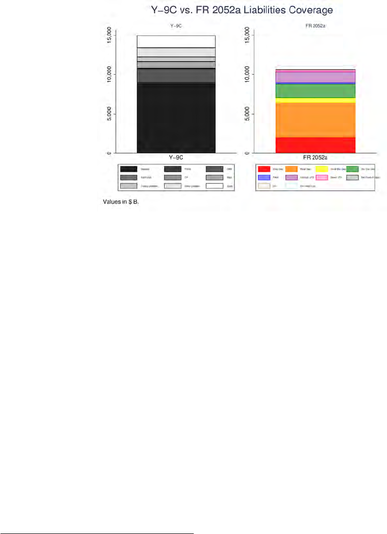
Figure A.1:

Y-9C vs. FR 2052a Total Liabilities Coverage.

Data Source: FR 2052a and FR Y-9C for

banks in the FR 2052a monthly panel.

We note only one institution with a deviation of more than 10% between the two reports in any

quarter.

Importantly, we do not try to reconcile loans reported in the FR Y-9C with those reported

in the FR 2052a, as this requires banks to report the lifetime cash ﬂows from a loan, which includes

both its principal and interest payments. This is in contrast to the FR Y-9C, which reports the book

(or market) value of bank loans.

We also make use of the FR Y-14Q, a conﬁdential supervisory data set maintained by the Federal

Reserve to assess capital adequacy and to support stress testing. The FR Y-14Q data contain detailed

quarterly data on: various asset classes, capital components, and categories of pre-provision net

revenue. These data are for US bank holding companies, intermediate holding companies of foreign

banking organizations, and savings and loan holding companies with more than $100 billion in total

consolidated assets.

We primarily make use of the FR Y-14Q corporate loan and commercial real estate schedules to

analyze loan terms to C&I and CRE borrowers. For this purpose, the FR Y-14Q covers approximately

two-thirds of the bank C&I lending market (Chodorow-Reich et al., 2021). It includes key information

on loan-terms, including the utilized and committed amount each quarter, interest rate, interest rate

index (for ﬂoating rate loans), and interest rate ﬂoors and ceilings, if they exist. For some of our

analyses, we restrict our sample to a sub-sample of Y-14 loans. For our accounting counterfactal

analysis, we restrict our sample to domestic C&I and CRE loans so we can compare estimated Y-14

revenues to Y-9C call report income for the same line item. In most of our analyses, we include

Speciﬁcally, we compare total deposits and wholesale funding that we source from the FR 2052a to Total Liabilities less

Other Liabilities less Trading Liabilities less Repo in the FR Y-9C to construct a like-for-like comparison. We also compare

component balances to the extent possible. For deposits speciﬁcally, we note only a single bank-quarter observation with

a > 5% deviation between the FR 2052a and the FR Y-9C. The remaining deviations are expected, as values reported in

the FR 2052a reﬂect contractual cash ﬂows, while values in the FR Y-9C reﬂect balance sheet book values, which can be

adjusted for various accounting reasons, such as securities recorded at fair value.

The size cutoff is based on: “(i) the average of the ﬁrm’s total consolidated assets in the four most recent quarters as

reported quarterly on the ﬁrm’s Consolidated Financial Statements for Holding Companies (FR Y-9C); or (ii) if the ﬁrm has

not ﬁled an FR Y-9C for each of the most recent four quarters, then the average of the ﬁrm’s total consolidated assets in the

most recent consecutive quarters as reported quarterly on the ﬁrm’s FR Y-9Cs.” Prior to 2020Q2, the respondent panel was

composed of any top-tier BHC or IHC with $50 billion or more in total consolidated assets.

loans secured by owner-occupied real estate (which are reported on the Y-14Q C&I schedule) with

other loans secured by real estate (loans reported on the Y-14Q CRE schedule) to align with the Y-9C

reporting aggregation.

We also use the FR 2420 data collection to analyze bank funding costs prior to and at the onset

of the COVID pandemic. This conﬁdential report is ﬁled daily by US banks with greater than $18

billion in assets, and contains transaction-level information for bank wholesale Certiﬁcate of Deposit

(CD) and time deposit issuances of greater than $1 million, including interest rate, maturity term,

and counterparty type. It also includes transaction-level information for selected deposits of greater

than $1 million and with a maturity between 1 and 7 days. In our analyses of interest rates at the

onset of the COVID pandemic, we compute period-speciﬁc interest rates as volume-weighted means

or medians among banks that reported transactions during that period. For overnight deposit rates,

we include all transactions with the relevant counterparty (for example, bank, NBFI, or non-ﬁnancial

corporate) that have a term of 1-day. For 3-month wholesale deposit rates, we include all transactions

with the speciﬁed counterparty that have terms between 89- and 92-days. This includes transactions

from banks that are both within and outside our main sample from the FR 2052a and FR Y-14

bank-level results.

For publicly available interest rates, including LIBOR and SOFR, we source data from FRED. We

source OIS, BSBY, and term SOFR rates via Bloomberg. Interest rates for Federal Home Loan Banks

(FHLBs) are not publicly available for all 11 FHLBs. We rely primarily on the publicly available

FHLB Des Moines historical rate ﬁle. However, we compared these rates to other publicly available

FHLB rates for the ﬁrst six months of 2020 (FHLB Boston and FHLB Pittsburgh) and note that these

rates follow similar trends during the pandemic, after adjusting for required investment in FHLB

activity-based capital and dividends that FHLBs pay on those investments.

We adjust for FHLB dividends and for the cost of holding FHLB activity-based capital stock in a

way similar to Ashcraft, Bech, and Frame (2010),

using the formula:

Adjusted Rate

= r

× (1 − h) + (h × LIBOR

) − (c ∗ (1 − h) ∗ d)

+ (c ∗ (1 − h) ∗ (1 − CET1 ∗ rw) ∗ LIBOR

) + (c ∗ (1 − h) ∗ CET1 ∗ rw ∗ ROE),

where

Adjusted Rate

is the all-in FHLB rate,

is the notional FHLB rate for a given term

the collateral haircut,

LIBOR

is the LIBOR rate for term

is the FHLB’s activity-based capital

requirement,

CET1

is a bank’s minimum CET1 ratio target,

is the risk weight that banks must

apply to FHLB stock, and ROE is the bank’s cost of equity (the ROE target). In essence, this formula

captures the all-in interest rate for funding a dollar of collateral via the FHLB. We assume that the

collateralized portion of the advance is funded at the FHLB notional rate (ﬁrst term) and that the

un-collateralized portion of the FHLB advance is funded via LIBOR (second term). We also account

for the bank’s requirement to purchase additional FHLB activity-based capital that is partially funded

by unsecured funding at LIBOR (fourth term) and partially funded by equity at the bank’s ROE

target (ﬁfth term). We also reduce the rate by the value of expected dividends that the bank receives

from the FHLB for its activity-based capital purchase (third term).

Details on our assumptions vary between the GFC and COVID period because collateral haircuts,

activity-based capital requirements, and dividend expectations have changed since the GFC. To

account for these time-varying parameters, we leverage the FHLB Des Moines historical dividend ﬁle,

which reports quarterly dividends on activity-based capital since 2000. We use the prior quarter’s

dividend rate in our calculations for the current quarter’s “All-in” rate. We also assume the existence

of a 4.45% activity-based stock purchase requirement until 2013, when SEC ﬁlings show that the

requirement decreased to 4%. For both periods, we assume a static 19% collateral haircut. We also

We build on this adjustment by also including factors to adjust for the cost of capital for holding FHLB activity-based

capital.

account for the incremental cost of capital to purchase FHLB stock using static adjustment parameters:

15% minimum bank CET1 ratio, 20% FHLB stock risk weight, and 15% ROE target.

We source additional bank-level information from the FR Y-9C and bank call reports, which

are public and reported quarterly. These reports include information on bank assets, capital ratios,

and quarterly interest income and expenses. For certain ﬁelds reported only in the call reports, for

instance small business loans, FHLB advances, and interest income on C&I loans, we aggregate

across all bank subsidiaries to estimate exposure at the holding company-level.

We obtain aggregate time series from FRED on bank assets and liabilities during the GFC. We

focus primarily on asset and liability series for large domestically chartered banks, and adjust these

for large non-bank mergers based on public notes on the Fed’s H8 series.

We also use data from S&P Compustat and Capital IQ to conduct ﬁrm-level analysis of drawdowns

during the COVID recession and the GFC. We source standard ﬁnancial statement variables, including

cash (CHQ), cash and equivalents (CHEQ), annual operating cash ﬂow (OANCFY), annual cash

dividends paid (DVY), and annual long-term debt issuance (DLTISY) from Compustat. We source

credit lines outstanding (IQ_RC) from Capital IQ. As credit lines outstanding are only reported on

an annual basis for most ﬁrms during the GFC, our main cross-sectional GFC analysis is conducted

at an annual frequency. In some analyses (for example, Table 4), we also ﬁlter, based on data quality

in Capital IQ, by restricting our sample to a sub-sample of ﬁrms for which we are able to match

long-term debt between Compustat (DLTTQ) and Capital IQ (IQ_TOTAL_DEBT - IQ_ST_DEBT)

within 10%, on average.

B Heterogeneity in Bank Funding Costs

This section provides further details on the calculation of heterogeneity in bank funding costs, with a

focus on the incremental funding costs of regional banks.

To estimate the heterogeneity in bank short-term funding costs, we use secondary market

transaction data from TRACE and FISD/Mergent between July 2002 and July 2021 for our sample of

large banks. We source these data via WRDS, using a cleaned version of merged TRACE/Mergent

data, aggregated to the monthly level at the instrument-level. The WRDS-cleaned version of this data

set has several advantages over the raw data, including the de-duplication of trades that are reported

by both buyer and seller, and the removal of canceled trades and variable-rate securities. We further

restrict our sample of transactions by dropping securities that are subordinated or convertible. We

restrict our focus to instruments with a remaining maturity of between 3 months and 3 years.

We calculate instrument-level yield spreads as the difference between the trade-weighted yield on

the instrument and the maturity-matched constant-maturity US Treasury yield.

We then estimate

the following equation via weighted least squares:

ibt

= β

+ β

ibt

+ β

+ δ

+ e

ibt

, (14)

where

i,b,t

is the yield spread on instrument

issued by bank

trading at time

ibt

is the remaining

maturity on that instrument in month

is an indicator variable bank set to 1 if and only if bank

is listed in Table A.1 as a regional bank, and

is a month ﬁxed effect. A summary of the results

of this regression are in Table B.1, for three different sample periods. The results suggest that the

unsecured wholesale funding costs of regional banks are about 22 basis points higher than those of

For comparison, in December 2019 the median call report bank had a 15% CET1 ratio and 10% ROE.

We interpolate between the yield on 3-month and 3-year US Treasuries, based on the remaining maturity of the bank

debt instrument. For instance, a bank note with remaining maturity of 6 months would be spread against a rate that is

the 3-month US Treasury rate and

the 3-year US Treasury rate.

the largest banks in our sample, post-GFC (Column 2), and about 10 basis points higher since 2015

(Column 3).

These results are based on weighted-least-squares (WLS) estimation, with a weight on the squared

residual

ibt

that is proportional to the total trade volume

ibt

of instrument

during month

. This

is the optimal linear unbiased estimator (generalized least squares) under the assumption that the

noise terms

ibt

}

are uncorrelated and that the variance of

ibt

is proportional to the inverse of the

trade volume of instrument

in month

. Ordinary least squares (OLS) estimation generated a much

poorer ﬁt, a much higher

-value, and a counter-intuitive negative sign for the estimated coefﬁcient

, the slope of the term structure of yield spreads.

Table B.1: Heterogeneity in Bank Funding Costs.

Variable (1) (2) (3)

Remaining Maturity 0.2137 0.2486 0.146

[0.0002] [0.0] [0.0]

Regional Indicator 0.015 0.2227 0.1053

[0.79] [0.00] [0.00]

Sample Full Post-GFC Recent

Reg Type WLS WLS WLS

0.0014 0.0796 0.1432

N 39279 24560 12773

Notes: The table summarizes estimates of model

(14)

obtained by weighted-least-squares (WLS), with a weight on the

squared residual

ibt

that is proportional to the total trade volume

ibt

of instrument

during month

. The

shown

corresponds to the weighted sum of squares. The

-values shown are rounded to two signiﬁcant ﬁgures and estimated

with heteroskedastic robust standard errors, and reported in brackets. The “Full" sample period (Column 1) is July 2002

to July 2021. The Post-GFC period (Column 2) is January 2010 to July 2021. The “Recent” sample period is January

2015 to July 2021.

C Incitements to Draw Early or to Run

The following extension addresses a borrower’s incentives to draw on its credit lines even before they

are needed, and when drawing to deposit the resulting funds at the same bank. These incentives

are inﬂuenced by the combined effects of potential future deteriorations in the credit qualities of the

bank or the borrower. Ideally, we want to capture the following incentives:

There is a relationship beneﬁt or convenience to keeping drawn funds on deposit in the same

bank.

If the bank’s credit quality is at risk of worsening signiﬁcantly, the borrower has an incentive to

maintain liquidity by drawing early and placing the funds in another cash instrument, such as

deposits in a different bank. This could be part of a run on the bank.

If the borrower’s or the bank’s credit quality is at risk of worsening signiﬁcantly, the borrower

has an incentive to draw on the line early, before the bank blocks the borrower from doing so

by claiming that the borrower has not met the necessary covenants. If the bank’s credit quality

were to deteriorate signiﬁcantly, then the bank has an incentive to block the drawing on lines to

preserve its liquidity, even if the borrower’s quality has not deteriorated, in which case there is

an associated relationship cost to the bank.

First, however, we ignore for simplicity the borrower’s credit risk, which makes the problem

complicated.

Lines are contracted at time 0, giving the borrower the option to draw on the line at time 1 or at

time

at an interest rate equal to a ﬁxed contractual spread

over the reference rate. We analyze

cases in which the reference rate is either a credit-sensitive rate like LIBOR or a risk-free rate

SOFR. Purely for notational simplicity, given the increased model complexity, we assume that the

risk-free rate

is always zero. The reference rate is

for loans taken at time 1 and maturing at time

, and

for loans taken at time

and maturing at time 2. We ignore risk aversion throughout. For

the case of credit-sensitive reference rates, we take

and

to be positively correlated with the

unsecured borrowing rates of the bank, r + S

at time 1 and r + S

at time a.

The borrower will be blocked from drawing at time

≥

, for some threshold

. Because we

are conducting a marginal analysis, we take

as given, although it may depend on the borrower

type. The spreads

and

are afﬁliated, so the conditional probability at time 1 that the borrower is

blocked from drawing at time

is increasing in

. The borrower will endogenously choose whether

to deposit any funds drawn at time 1. Any drawn funds outstanding at time

are for uses by the

borrower at that time, and are not left on deposit. If the borrower does not need cash at time a, any

previously drawn funds are repaid.

At time 0, the bank offers the borrower a menu

{(L

s) : L ≥

}

of credit line terms distinguished

by the size

of the line and the associated ﬁxed spread

over the variable loan benchmark rate

At time 1, information reveals the credit spread

of the bank for unsecured wholesale funding

maturing at time

. Likewise, at time

, the credit spread

of the bank for loans maturing at time 2

is observed. Information is symmetric throughout.

The borrower will use the drawn funds only at time

, if at all. At time

, the beneﬁt to the

borrower of having access to

in cash is

b(x

ψ)

, where

is a liquidity-preference variable that is

revealed at time 1 and

is a function with the same properties assumed in the basic model. At time 1,

given the committed size

of the credit line, the borrower chooses the amounts

to borrow at time

1. At time

, the borrower chooses the incremental amount

to borrow, if not blocked by the bank,

so as to maximize the beneﬁt of access to the cash, net of the present value of the loan repayment. We

allow

to be negative, subject to

+ q

≥

0, with the idea that by time

, the borrower will either

have used the drawn funds or paid back funds drawn at time 1. At time 2, the total assets and total

liabilities of the bank are revealed and the bank is either solvent or not. For simplicity, the bank will

not default before time

, for example because the bank has no liabilities maturing before time 2. If

solvent at time 2, the bank pays back

(

+ S

)(

+ S

) + q

(

+ S

)

. The corporate borrower repays

the outstanding loan amount,

+ q

, whether or not the bank is solvent at time 2. The proportional

reputational or convenience cost to the borrower of not leaving the drawn funds on deposit at the

same bank is

. For simplicity, we assume that the borrower will not default on the credit line and

take

= r + S

. We don’t take

= r + S

, because we want to allow for the risk that the bank will

become much worse at time

than “LIBOR quality,” which as a result could prevent the borrower

from drawing or even make the bank unable to fund the draw request.

State by state, the borrower thus solves

V(L) = sup

0 ≤ q

≤ L, W

[

b(Q + q

, ψ) − Wq

e − Q(1 + R

+ s)( 1 + R

+ s) − q

(1 + R

+ s) | S

, ψ

]

(15)

where q

is constrained to be non-positive on the event {S

≥

S}, where

Q = q

(H + (1 − H)W),

and where

is the indicator of the event that the bank honors its deposit obligation at time

. We

take

P(H | S

)

to be a simple given function, for example linear, assuming that

has a sufﬁciently

bounded range. Or, for another example, we can take

H =

∗

}

, where

∗

is a threshold above

As reﬂected in

(15)

, if the borrower loses its deposits at time

, then of course it is not obligated to

pay back the loan.

The problem can be solved inductively as follows. At time

, for each given amount

of funding

obtained at time 1, the optimal incremental borrowing amount

is the solution of the associated

Kuhn-Tucker conditions, which have an explicit ﬁrst-order interior condition whenever the solution

is interior. We can thus treat

as an explicit function of variables observable at time

. We ignore for

now cases in which the fraction

of withdrawn cash may interior, and take

to be chosen as zero

or 1 for simplicity. Then, given

and

, the optimal amount

of funding at time 1 can be solved

by a line search for each of two cases,

W =

0 and

W =

1. The better of these two cases determines

and q

, state by state, and from these, q

The marginal increase at time 1 in the equity value of the bank associated with given contractual

credit line terms (L, s) is

L,s

= E

(

[(1 + R

+ s)( 1 + R

+ s) − 1] + q

+ s) − q

((1 + S

W)(1 + S

) − 1) − q

]

)

(16)

where 1

is the event of bank solvency at time 2. The ﬁrst two terms inside the expectation of

(16)

are the bank’s proﬁt markups. The third and fourth terms are debt overhang costs to shareholders.

For each line size

, the bank offers a competitive spread

at which the bank’s shareholders break

even on marginal new credit lines, meaning that

L,s

0. Given the resulting menu of feasible line

terms, the borrower solves (15) for the optimal line amount L

∗

D Model Calibration Details

This section of the appendix provides additional details on the calibration of the theoretical model.

The main goal of the calibration is to match the aggregate quarterly credit line drawing behavior

from the ﬁrst quarter of 2015 to the second quarter of 2021. We ﬁrst provide some properties of the

model used in the calibration. In the following, we let e = −e .

Theorem 1.

For a given credit line limit

, the optimal quantity

Q(L)

of drawn credit has the following

properties.

1. On the event {K(W) + e > 0, K(W) + e < L((1 + R + s)

E[Q(L) | W] = υ

L(K(W) + e − L(((1 + R + s)

))

( e − e)

+ υ

− max(0,

(K(W)+e)

(1+R+s)

)

+ min(L,

(K(W)+e)

(1+R+s)

)

2(e−e)

(1+R+s)

+ (1 − υ) min

(K(W) + e

)

(1 + R + s)

2. On the event {K(W) + e

≤ 0}, we have E[Q(L) | W] = 0.

On the event

{K(W) + e ≤

}

and

{K(W) + e

}

, we have

E[Q(L) | W] = (

− υ) min(L

(K(W)+e

)

(1+R+s)

)

4. On the event {K(W) + e ≥ L(1 + R + s)

}, we have E[Q(L) | W] = L.

Theorem 2.

For a given credit line limit

, the cumulative distribution function

of the cross-sectional

distribution of credit line utilization has the properties

F(0) = P(Q(L) = 0 | W) =











1 on the event K(W) + e

≤ 0

1 − υ on the event K(W) + e ≤ 0 and K(W) + e

> 0

0 on the event

(K(W)+e)

(1+R+s)

≥ 0

−

(K(W)+e)

e−e

otherwise,

and

F(L) = P(Q(L) = L | W) =











1 on the event

(K(W)+e)

(1+R+s)

≥ L

0 on the event

(K(W)+e

)

(1+R+s)

< L

1 − υ on the event

(K(W)+e)

(1+R+s)

≤ L and

(K(W)+e

)

(1+R+s)

≥ L

e−L((1+R+s)

+K(W)

−e+e

+ 1 − υ otherwise.

Motivated by calibrating the model so as to match the aggregate utilization of credit lines observed

in our sample, we assume the following functional form for the function

K(·)

that determines the

macro component K(W) of borrowers’ liquidity shocks:

K(x) = C

+ C

min(x, x

) + C

(x − x

)

1 + e

−C

(x−x

)

, (17)

for some constants

, and

to be calibrated. This functional form captures the

features of the data that borrowers sharply increased their total draw-down quantity during the

COVID shock when LIBOR-OIS rose to around

140 basis points, the level at which drawing

sharply increases for the median borrower. The sensitivity to LIBOR of this increase is captured by

the parameter C

We calibrate the model in the following steps

For any parameter choices

P = (M

υ)

, we can calculate the

bank’s marginal improvement in equity value per credit line when the equilibrium spread is

as,

Π(P, s) = E[(1 − 2W)δE[Q(L) | W](s + W − κ(W)W)],

by numerical integration with respect to the probability density of W.

2. Fixing P, we solve s(L) with a numerical binary search for the solution to

Π(P, s(L)) = 0.

3. Let

shock+

= (M, C

, C

, x

, 1.1L, e, e

, υ)

and

shock−

= (M, C

, C

, x

, 0.9L, e, e

, υ).

We solve s(1.1L) and s(0.9L) such that

Π(P

shock+

, s(1.1L)) = 0

and

Π(P

shock−

, s(0.9L)) = 0.

We ﬁx a credit line fee

of 20 basis points. We solve for the line size

that maximizes a

borrower’s expected net beneﬁt, using numerical integration. This expected beneﬁt, for each of

three parameter choices, is

U(P, L, s(L) ) = E



(K(W) + e)

1 − α

Q(L)

1−α

) − Q(L)δ(1 + R + s(L))



− f L

U(P

shock+

, 1.1L, s(1.1L)) = E



(K(W) + e)

1 − α

Q(1.1L)

1−α

) − Q(1.1L)δ(1 + R + s(1.1L))



− 1.1 f L

U(P

shock−

, 0.9L, s(0.9L)) = E



(K(W) + e)

1 − α

Q(0.9L)

1−α

) − Q(0.9L)δ(1 + R + s(0.9L))



− 0.9 f L.

In equilibrium, borrowers choose a line size L with the property that Ξ(P) = 0, where

Ξ(P) = max(U(P

shock−

, 0.9L, s(0.9L)), U( P

shock+

, 1.1L, s(1.1L)), U( P, L, s(L))) − U(P, L, s(L)).

For the realization

of LIBOR-OIS observed in the data in quarter

, we solve the equilibrium

assuming that the equilibrium

and

are the actual spread and credit limit observed in the

historical data. From this, we calculate the modeled aggregate amount drawn,

∗

( P ) =

M · E[Q(L) | W = w

]

. The empirical analogue is the actual aggregate quantity

drawn in

quarter

. Likewise, we compute the modeled fraction of borrowers utilizing their entire credit

line, which is

∗

( P ) = P(Q(L) = L | W = w

)

. As an approximation of the precise empirical

analogue to

∗

, we take the empirical analogue to be the fraction

of lines that were drawn in

quarter

to within 95% of their line limits. We also calculate the average across sample periods

of the total across borrowers of credit line sizes in the data. This average is denoted L

sum

Because

is conditionally uniformly distributed with probability

, we know that for any

and

in {0, 1, 2, 3, 4, 5, 6, 7, 8},

m,∗

( P ) ≡ P



Q(L) ∈



ιL

( ι + 1)L





W = w



= P



Q(L) ∈



( ι

+ 1)L





W = w



In the data, we observe the fraction of borrowers with line utilization between

(

80l

)

and

(

80(l+1)

)

% for each

l ∈ {

1, 2, 3, 4, 5, 6, 7, 8

}

. These empirical fractions are roughly the

same across these “interior” deciles. For each quarter, we calculate the average of these interior

fractions, denoted Z

As a ﬁrst step in calibrating the model, we choose the model parameters

that minimize the

sum of squared model errors, deﬁned by

( P ) = Ξ(P)

+ (L

sum

− M · L)

∑

i=1

∗

( P ) − Q

)

∑

i=1

∗

( P ) − Z

)

∑

i=1

m,∗

( P ) − Z

)

Here, we abuse the conditional-expectation notation by using a regular version

w 7→ E[ Q(L) | W = w]

of the conditional

expectation, a function that exists under a mild technical integrability condition.

where the summation over i is across all N quarters in our 2015-2021 sample period.

Minimizing the unweighted sum

( P )

does not account for the quite different magnitudes

of the different types of terms in the sum. This could result in heavily overweighting some

types of model errors over other types. So, we perform a second calibration step by using the

ﬁrst-step parameters P

to estimate the error moments

≡|Ξ(P

) |

≡|L

sum

− M

· L|

≡

−1

∑

∗

( P

) − Q

)

≡

−1

∑

∗

( P

) − Z

)

≡

−1

∑

m,∗

( P

) − Z

)

where M

denotes the quantity of borrowers associated with P

Our ﬁnal model parameters

∗

are those minimizing the weighted sum of squared model

errors,

( P ) =

Ξ(P)

sum

− M · L)

∑

i=1

∗

( P ) − Q

)

∑

i=1

∗

( P ) − Z

)

∑

i=1

m,∗

( P ) − Z

)

At the ﬁtted parameters, the ﬁrst term is zero, so in fact plays no role in determining the ﬁtted

model.

10.

It turns out that

is not well identiﬁed in our sample, because LIBOR-OIS spreads vary within

our sample by no more than 150 basis points, but

is 140.6 basis points. We ultimately chose

80 so that the modeled line utilization during the GFC is roughly 7% more than the

maximum sample utilization in non-crisis sample periods for which LIBOR-OIS is 80 basis

points or less. We experimented with a wide choice of

and found that our main results are

quite robust to this choice.

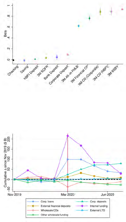
E Additional Tables and Figures

Figure E.1:

Bank Funding Rates and LIBOR

Notes: This table displays the coefﬁcient on 3M LIBOR-OIS in a regression of the form

= β × [LIBOR

− OIS

] + e

, where y

is the interest rate or OIS spread on date t. Table E.3 in the Appendix also shows the corresponding detailed regression output. Conﬁdence

intervals calculated from robust standard errors. Series represent different maturities and different start dates, which are further detailed in Table E.3. Checking and Saving series

represent demand deposit rates. NBFI, Bank and Corporate Deposit are spreads over the effective fed funds rate. 3M SOFR, 3M “All-in” FHLB Advance, 3M CD (corporate), 3M CD

(NBFI), and 3M BSBY represent spreads over 3M OIS.

Figure E.2:

Corporate Drawdowns and Funding Sources: U.S. Operations of Foreign Banking

Organizations (FBOs). Data Source: FR 2052a. This ﬁgure shows the evoluation of aggregate assets and liabilities during the COVID pandemic for the

consolidated US branches of a balanced panel of 14 FBOs: BARC, BNPP, TD, SOGN, DB, UBS, BMO, BBVA, KN, CS, MUFG, SMBC, MFG, and RY. Values represent cumulative

growth/decreases compared to the starting month in $ billion.

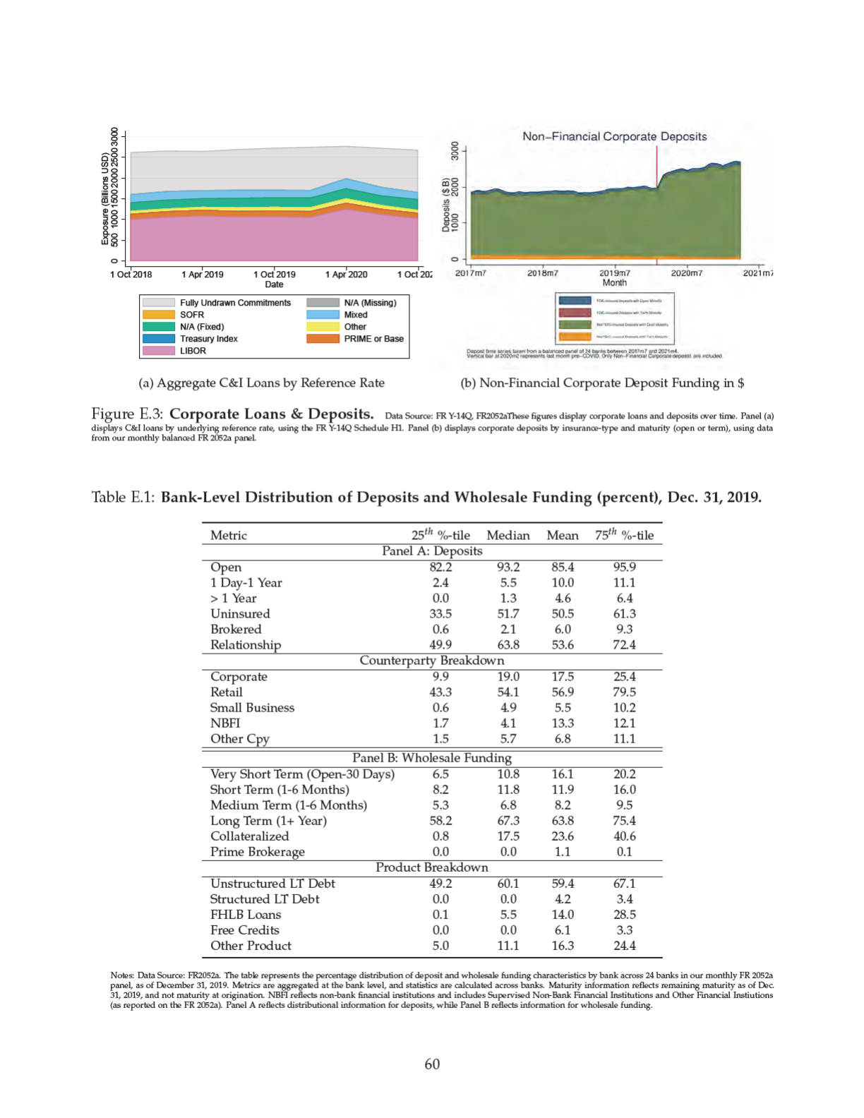
Table E.2: Bank-Level Distribution of Floating Rate Long-Term Debt

in % Industry Mean 25

% Median % 75

% No. Banks

Fixed 69.93 78.24 69.70 78.56 88.73 14

Floating 29.02 21.51 11.27 21.34 30.30 14

LIBOR 11.36 11.94 8.97 10.82 18.67 14

SOFR 11.34 5.70 0.00 0.00 9.67 14

This table displays statistics from the cross-sectional distribution of banks for which we were able to “conﬁdently" source

long-term debt issuance terms via Bloomberg. Data are as of June 30, 2021. We deﬁne our “conﬁdence" by measuring

the bank-level difference between outstanding amounts as reported in Bloomberg and borrowings as reported in the FR

Y-9C. Borrowing in the FR Y-9C is deﬁned as other borrowed money plus subordinated debt less advances from FHLBs.

“Conﬁdence” is deﬁned as matching Y-9C within 10% or matching non-deposit liabilities within 5%. Floating rate debt

includes both current ﬂoating rate notes, as well as variable notes (which start paying ﬁxed and convert to ﬂoating at a

future date).

Table E.3: Interest Rate Correlations with LIBOR-OIS

Deposit & Risk-Free Rates

Checking Saving ON Corp ON NBFI ON Bank SOFR

LIBOR-OIS -0.01 -0.01 0.09*** 0.01 0.05*** 0.04***

(0.01) (0.02) (0.01) (0.01) (0.01) (0.01)

N 447 447 696 696 693 615

Start Date 14 May 2009 14 May 2009 01 Oct 2018 01 Oct 2018 04 Oct 2018 03 Jan 2019

Wholesale Rates

FHLB FHLB Adj. Fin. CP Corp. NBFI BSBY

LIBOR-OIS 0.51*** 0.62*** 0.77*** 0.88*** 0.89*** 0.93***

(0.01) (0.01) (0.01) (0.04) (0.02) (0.01)

N 4875 4875 4639 1340 1385 1351

Start Date 04 Dec 2001 04 Dec 2001 04 Dec 2001 15 Jan 2016 11 Jan 2016 06 Jan 2016

This table displays the coefﬁcient on LIBOR-OIS in regressions of the form

= α + β × LIBOR-OIS

+ e

where Y

is the interest rate or OIS spread on date t. The rates displayed in this table are: Interest and Savings Rate, sourced from FDIC calculations using RateWatch Data; overnight

corporate, non-bank ﬁnancial, and bank deposit spread vs. effective fed funds, where O/N rates are calculated by counterparty type from FR 2420 data; 3M term SOFR and 3M

BSBY spreads to 3M OIS, sourced from Bloomberg; 3M Financial CP-OIS spread, sourced from FRED; the 3M FHLB Des Moines rate on ﬁxed rate advances spread to 3M OIS; and

the average 3M non-ﬁnancial corporate CD and non-bank ﬁnancial CD rates, calculated from the FR 2420, spread to 3M OIS. Regression coefﬁcients can be interpreted as the average

relationship between LIBOR-OIS and the corresponding rate or spread. Note: The relatively low observation count for savings and checking deposit rates is due to the weekly nature

of the data series, compared to other series, which are reported daily.

Table E.4: Floating Rate Loans at Large US BHCs (as of December 31, 2019)

(in %) Industry Bank Holding Company No. of

25th Median 75th Banks

Panel A: Credit Lines

% LIBOR 70.51 53.75 74.95 84.79 20

% Prime 6.92 2.51 5.07 9.22 20

% Fixed 6.22 0.52 2.52 6.75 20

% Other 16.36 9.36 13.82 32.14 20

Panel B: Term Loans

% LIBOR 72.80 51.73 84.01 89.88 20

% Prime 4.15 0.10 0.83 1.64 20

% Fixed 14.99 4.74 12.65 17.84 20

% Other 8.05 0.58 1.60 5.57 20

Panel C: Commercial Real Estate

% LIBOR 65.61 54.82 75.06 83.27 20

% Prime 3.58 0.08 0.98 2.78 20

% Fixed 28.38 9.89 18.80 29.77 20

% Other 2.43 0.45 1.32 2.69 20

Panel D: C&I and CRE Loans

% LIBOR 68.49 62.21 75.37 80.75 21

% Prime 5.08 0.61 2.49 4.90 21

% Fixed 17.18 8.18 12.71 15.69 21

% Other 9.25 4.21 7.85 10.49 21

LIBOR Util. / Assets 7.39 1.99 10.81 20.38 21

LIBOR Util. / STWF 129.73 34.13 171.79 287.65 21

This table displays the distribution of ﬂoating rate loan terms across banks that ﬁle the FR Y-14Q Schedule H1 B (corporate loans) and FR Y-14Q Schedule H2 (commercial real estate).

In Panels A and B, we restrict our sample to domestic C&I loans only. In Panel C, we restrict our sample to domestic loans secured by real estate. In Panel D, we pool loans across

C&I and CRE schedules. We also exclude all holding companies that are owned by foreign (non-U.S.) banks. Data are as of December 31, 2019 and reﬂect utilized loans (and not

unfunded commitments). We deﬁne short-term wholesale funding (STWF) similarly to Bowman et al. (2020), as the sum of commercial paper, fed funds purchased, and large time

deposits with remaining maturity less than one year, as reported in the FR Y-9C. We add to their deﬁnition other borrowed money maturing in one year or less.