Predicting Premier League Final Points and Rank Using Linear

Predicting Premier League Final Points and

Rank Using Linear Modeling Techniques

By Junyuan Gao

Advisor: David Aldous

Index

Introduction -------------------------------------------------------------2

Description of Data ----------------------------------------------------3

Preliminary Analysis --------------------------------------------------4

Model Construction and Simulation---------------------------------6

Test and Model Selection---------------------------------------------11

Prediction --------------------------------------------------------------13

Future Developments ------------------------------------------------15

Conclusion ------------------------------------------------------------15

Reference ------------------------------------------------------------- 16

I. Introduction

Soccer, one of the most popular sports in the world, has its own fascination. Soccer

fans enchant in the tense and exciting moments of goals, especially those last-gasp goals

that determine the game result and then determine the final rank and points of teams.

For example, in the 2015-16 season of English Premier League, the dark horse team

Leicester, who just ascended to the Premier League in 2014-15 season, surprisingly beat

all the other teams and won the champion. This phenomenon reflects one of the most

charming part of soccer— complexity, which makes the game result hard to be

predicted.

Though soccer game results and team ranks are hard to predict, curious people

always want to figure out the keys to determine the game result for their own reasons.

Betting companies has to correctly, or as correctly as possible, predict the game results

and ranks since they have to design a series of odds that produce stable profit from

gamblers. Their methodology might be complex and various—from analyzing the

strength of two teams and the possible strategies of two coachs, to the choice of the

referee at the game day, the injury situation of two teams and both teams’ future

schedule, etc. Gamblers and sports fans want to predict the game results and ranks

correctly since gamblers want to predict correctly since gamblers want to earn money

from betting companies and gain pleasure from correctly predict their favorite club

winning the game and the seasonal championship. Restricted to the lack of information

and experience in the industry, they have to make prediction based on less parameters

such as general performance of two teams in this season(which can be easily obtained

from game table), historical game records and odds from betting companies.

As a statistician and a soccer fan, I mainly focus on predicting the game results

using statistical modeling techniques. I choose to predict the game results and the team

ranks in a very straight way—predicting the number of the goals for each team. The

reason I choose to predict the number of goals is that regardless what strategies that

coachs use or what types of the goals are, whenever a team achieve more goals than the

other, that team will win the game. Within each game result produced, I can easily

generate the results to make a final table contains team ranks and final points. The goal

of the project is to predict the final ranks and points of 2016-17 premier league season.

This goal will be achieved mainly in following steps:

(1) Data collection and re-organization in order to be used to construct prediction

models

(2) Several models will be evaluated and tested on 2015-16 season

(3) Select the one among those models

(4) Predictions will be made via the best model on selected in step(2)

II. Description of Data

The data that I used in this project are collected from github and

www.premierleague.com. I collected the detailed match data of 2015-16 premier league

season, which can be regard as my training set, from github and obtained the completed

game results and future game schedule of 2016-17 premier league season, which can

be regard as the prediction set, from www.premierleague.com. Moreover, all execution

on data is under R.

The original data is a data frame with 380 rows and 49 columns, in which each row

stands for full information of one game in 2015-16 season. The information contains

team names, managers of teams, general information(date, location, name of referee,

etc.) and detailed statistics(e.g. number of assists, number of goals, number of tackles,

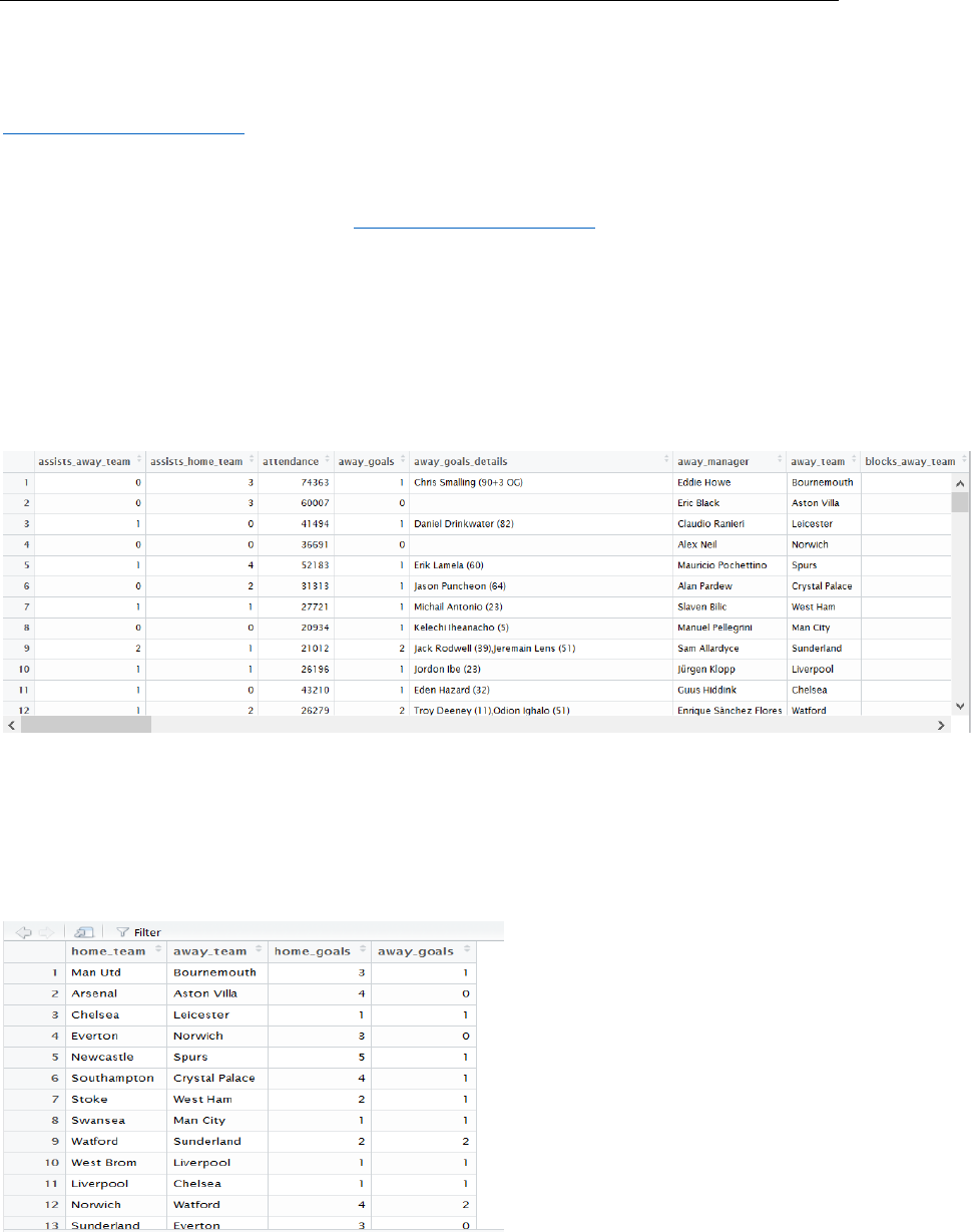
etc.). We can have a rough glance of the data in figure 1:

Figure 1: first 12 rows and 8 columns of original data frame

However, the data is too messy for the further research—as I mentioned in part I,

what I need is only the number of goals of home and away teams, so I simplify the

original data and produced the reduced data that only contains 380 rows and 4 columns,

which can be seen in Figure 2.

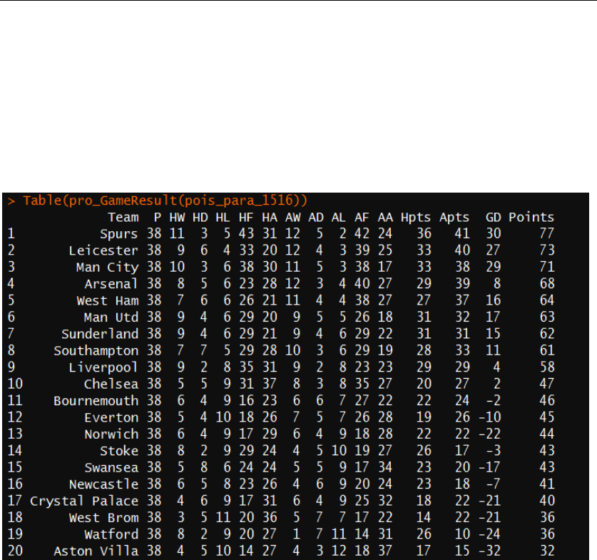
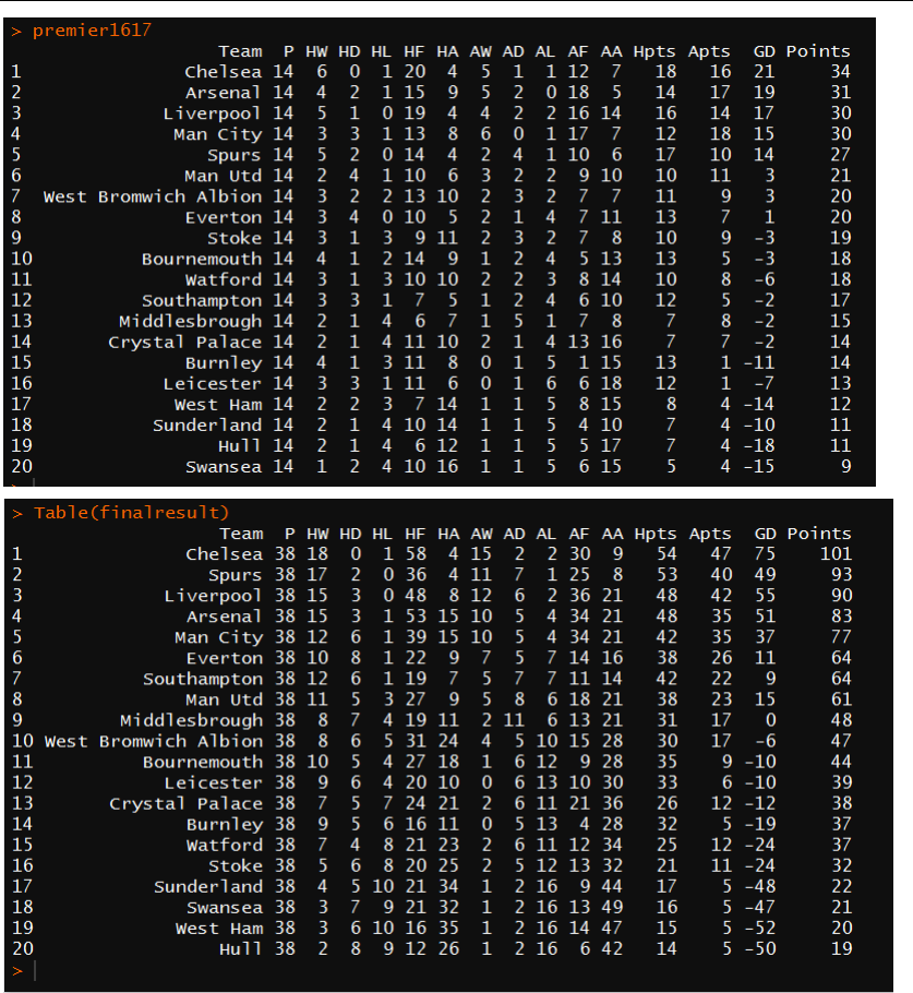
After obtaining the original match results in 2015-16 season, I created a function

Table() to generate the match results into a result table. Besides the similar statistics on

the other result tables, this table contains detailed statistics like the numbers of wins

that particular team play as home team and so on. The 2015-16 season table is shown

Figure 2: first 13 rows and

4 columns of reduced data.

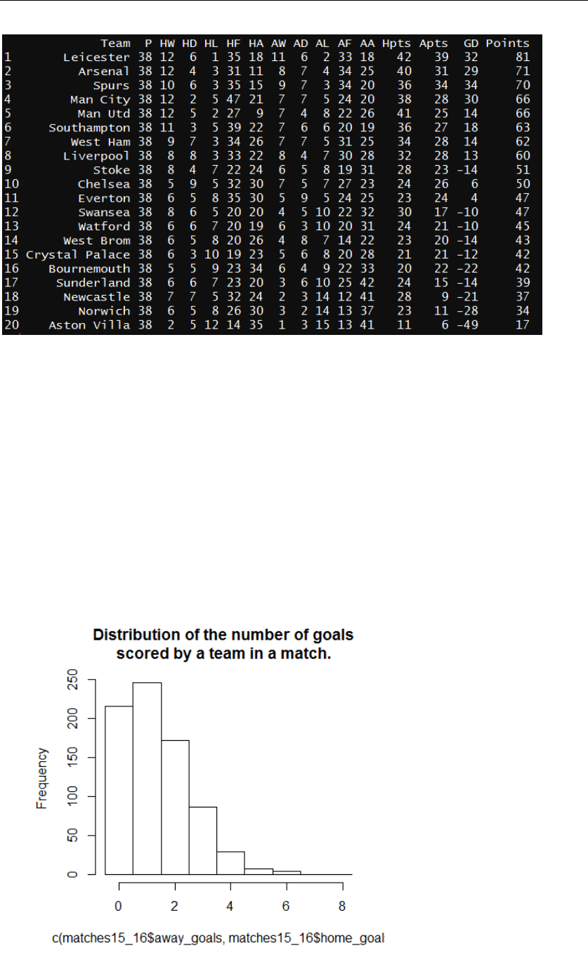
on Figure 3.

Figure 3: The detailed result table of 2015-16 Premier League season. P=number of matches played,

H= Home, A= Away, w=number of winning games, D=number of draw games, L=number of losing

games, HF/AF=Goal scored in home/away games, HA/AA= number of goals against in home/away

games, Hpts/Apts=points earned in home/away games, GD= goal difference.

By the same way, game results data and result table of 2016-17 season can also be

generated. Within this data, we are ready to step to the next part.

III. Preliminary Analysis

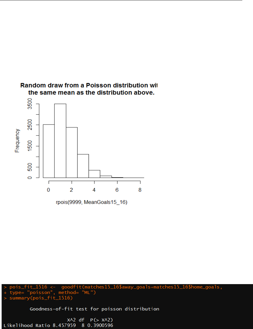
At first, I tried to figure out whether there is a trend, regardless of the difference

between home game and away game, of the number of goals in each match. The

following visualization can provide a directly perception:

Figure 4: Distribution of

numbers of goals of a team

in one match (regardless

the difference of home or

away)

Inspired by Rasmus Baath’s paper “Modeling Match Results in Soccer using a

Hierarchical Bayesian Poisson Model”, I realized that if we assume both teams have

equal probability of making a goal in each chance and both teams have many chances

in the equally long game time(90 minutes), the distribution of the number of goals

should follows a Poisson Distribution. To intuitively confirm this hypothesis, I plotted

a random draw of a Poisson Distribution whose mean is equal to the mean of number

of goals in each match and resulted in the following graph:

Observing Figure 4 and 5, we can easily detect that they looks really same, which

strengthen the power of this hypothesis. However, to officially check whether it’s true

or not, I made a hypothesis testing by using function goodfit() from package “vcd”. I

set the null hypothesis H

: The distribution of number of goals in one game is

approximately Poisson distributed. The test result can be viewed through figure 6:

Figure 6: Test statistics of goodness-of-fit test for Poisson distribution

This test statistics shows that X

= 8.457959 with 8 degrees of freedom and p-

value= 0.3900596, which indicates that the probability of the data follows the

distribution is approximately 39%. Though it looks a little bit small, it is quite

significant since our amount of data is also large. Just as Prof. Aldous noted: All models

are wrong but some are useful. Thus, by intuitively thinking, empirical observation and

Figure 5: Distribution of

results of random draw from

Poisson(mean= the mean of

goals scored in one match in

2015-16 season).

statistical test, I think that the test statistics could be a strong evidence to accept my null

hypothesis that the distribution of number of goals in each match in 2015-16 season

follows Poisson distribution.

IV. Model Construction and Simulation

After accepting the assumption of the number of goals in each match follows

Poisson distribution, I can start construct regression models based on the assumption.

In this part, two models are considered:

Model 1: Poisson regression separately on 2 parameters: home goals(Offence) and

away goals(Defence) of teams.

Model 2: Based on Model 1, consider an extra parameter—home advantage parameter.

Theoretically, the Poisson regression formula for this project can be represented as

Y=exp(Xβ), where Y is a vector of dependent variable that consists of the home goals

and away goals in games, X is a matrix of explanatory variables that records the home

and away teams corresponding to the games. β is a vector containing the parameters,

Offence and Deffence, of the model. Note that Y and β are at length 2n which is 2 times

of number of mathces since each of 20 teams has its Offence parameter and Defence

parameter, and each of the times will appear as either a home team or an away team.

Thus we can say Y and β are of the forms: Y=(y

i1, j1

, y

i1, j1

, …)

and β= (O

, …,O

, …,D

)

, where y

a,b

is the number of goals scored by team a versus team b in game

i; O

and D

stands for the Offence and Defence parameter of team j. To be specific, I

will show readers the structure with a naïve example:

Example: Assume we have 3 teams: Man Utd, Man City and Chelsea plays 3 games

pairwisely. Then we can write following table and representations:

Table 1: example of 3 games

Game

Home team

Away team

# of home

goals

# of away

goals

Man Utd

Chelsea

Man City

Man Utd

Chelsea

Man city

Hence, we have Y=(0, 3, 2, 2, 3, 1)

β=(O

, O

Che

, O

MC,

, D

Che

, D

MC,

)

and

MU Che MC MU Che MC







     

     

     

     

     

     







Game1

Game2

Game3

If we consider the home advantage parameter in model 2, our β and X will change

into β= (O

, O

Che

, O

MC,

, D

Che

, D

MC,

)

and

MU Che MC MU Che MC home







      

      

      

      

      

      







Moreover, to construct both model 1 and model 2 in practice, the following

guideline is considered:

(1) Estimate the Poisson parameters of each team based on the average amount of

home goals and away goals in each match.

(2) Produce a table of probabilities for the set of results possible for a football

match based on (1)

(3) Simulate game results of a season based on (1) and (2), then using bootstrap to

diminish the randomness

(1)

For the first step, I set the mean of the home/away goals of one team in the season

as its Poisson parameter , and create a function Y_beta_x() to calculate the Poisson

parameters. Inside the function, the build-in function glm() is used to calculate the

Poisson parameters. However, when dealing with model 2, I observed that the matrix

X in this case contains 41 columns while the rank is 40, which means that the glm

function will not produce a unique least square estimator of β. So I just modified the

function Y_beta_x() to make Y vector fit on X after reduced the 1

column.

Equivalently, we can write the Poisson regression R code as

glm(Y~ 0+ X_reduced_1

Column, family= poisson).

Within this modification, the number of columns of X is reduced to 40 and the

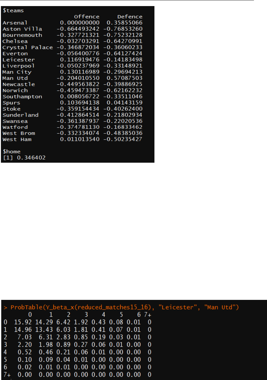
function will return a least square estimate of β. The result of the estimated parameters

in 2015-16 season is shown on Figure 7:

Game1

Game2

Game3

(2)

For the second step, I designed a function ProbTable() that produce a probability

matrix to show the probability of possible game result of two teams. The basic formula

to calculate the probability of a certain outcome is:

For team A, B whose number of goals scored are j and k, P(A v.s B has result j v.s

k)= P(# of goals of A= j) x P(# of goals of B= k).

For each team A, B whose number of goals scored are j and k, I used function

dpois() to obtain the probability P(A=j) under the Pois(O

- D

) distribution and obtain

the probability P(B=k) under the Pois(O

- D

) distribution. When using model 2, since

the home parameter is added, the distributions correspondingly change into Pois(O

+) and Pois(O

- D

). An example in figure 8 shows the probability matrix of the

possible outcomes of the game (in season 2015-16) between Leicester and Manchester

United:

Figure 8: The probability matrix of the outcomes of the game between Leicester City and

Manchester United(in percentage, e.g. 0-0 has 15.92% chance). The numbers 0~7+ on the row

indicates the possible number of goals of Leicester while the numbers on the column indicates the

number of goals of Manchester United.

Figure 7: Estimated Offence

and Defence parameters of

each teams as well as the

home advantage parameter

of model 2.

(3)

For the third step, I designed a function GameResult() to simulate the game results

for a whole season based on repetitively using the methods I mentioned in part (1) and

(2). After the game results of a whole season created, I used the Table() function

mentioned above to generate the game results into a final result table, which is more

clear and readable to readers. The following figure 9 is a nice example of the result of

one-time simulation of a whole season:

Figure 9: A result table of one-time simulation of games of the whole 2015-16 season of model 1

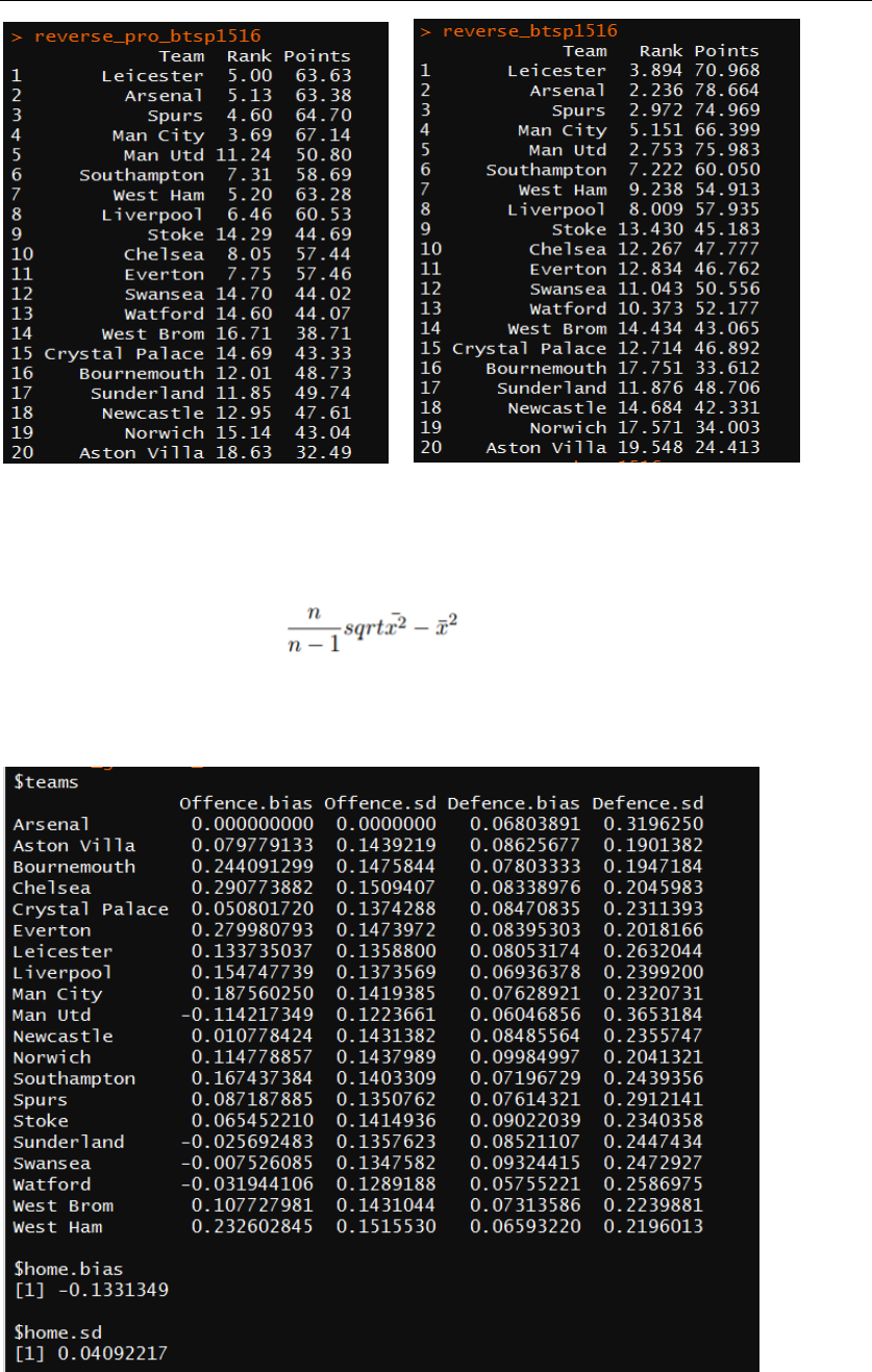
However, since one-time simulation might be badly affected by randomness, I used

the 1000 times bootstrap to produce game results of 1000 seasons and then take average

of them, which will weaken the effect of randomness. Since this part will mainly work

for the next section, only the bootstrapping game results, average rank and final points

are recorded after the bootstrap. Figure 10 is a comparison of average ranks and final

points between model 1 and model 2 after bootstrapping.

Figure 10: Comparison of average ranks and final points between model 1 and model 2 after

bootstrapping. Left: model 1 Right: model 2

Moreover, I created a function Accuracy() to calculate the bias= E(-_hat) and

the standard deviation dev= of every parameters of each team over

the bootstrap process. The smaller the bias and standard deviation are, the less

randomness does the simulation have. Figure 11 is the generated result of bias and

standard deviation of model 2 after 1000-times bootstrapping:

Figure 11: bias and std deviation of parameters model 2 over 1000-times bootstrapping

From the figure, we can see that the standard deviation for most of parameters are

less than 0.30, which is a very small number and indicates that the set of parameters

using the original ones are very closed to the original estimators I got in part (1).

Furthermore, the bias values also appears to be very small, which shows that little bias

occurred during the 1000-times bootstrapping process. Both the results of bias and

deviation reflect that my method of estimating parameters is doing well, and

surprisingly, the low bias and standard deviation of home parameter indicates that the

home advantage parameter is useful.

V. Test and Model Selection

The object of this section is to select the best model based on the real world result

of 2015-16 Premier League season. In order to choose the best model for the future

prediction, I designed three tests to determine which model is optimal.

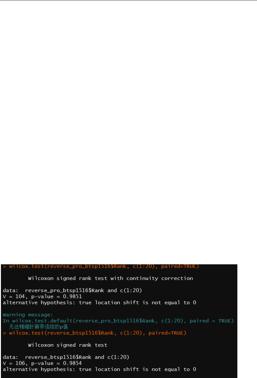
(1)

The first test is the non-parametric Wilcoxon rank sum test on team ranks and final

points towards model 1 and model 2. Observing and comparing figure 10 and figure 3

by eye, we can see that both 2 models have a nice prediction of the top 6 rank teams

and the bottom 3 rank teams towards the real-world result. However, it’s hard to

determine the goodness of simulation of those middle-ranked teams. By using

Wilcoxon rank sum test, I can quantitatively determine the rank sum of two simulated

tables and figure out its goodness of simulation. I set the null hypothesis H

: The

simulation ranks does not shift from the real-world ranks and test result is shown on

figure 12.

Figure 12: Wilcoxon rank test statistics for model 1(above) and model 2(bottom)

Looking at the test statistics of two models, I saw that they are really same: both of

them fail to reject null hypothesis due to the really large p-value, and there is nearly no

difference between their rank sum and p-value. To classify the best model more

efficiently, I designed the second test.

(2)

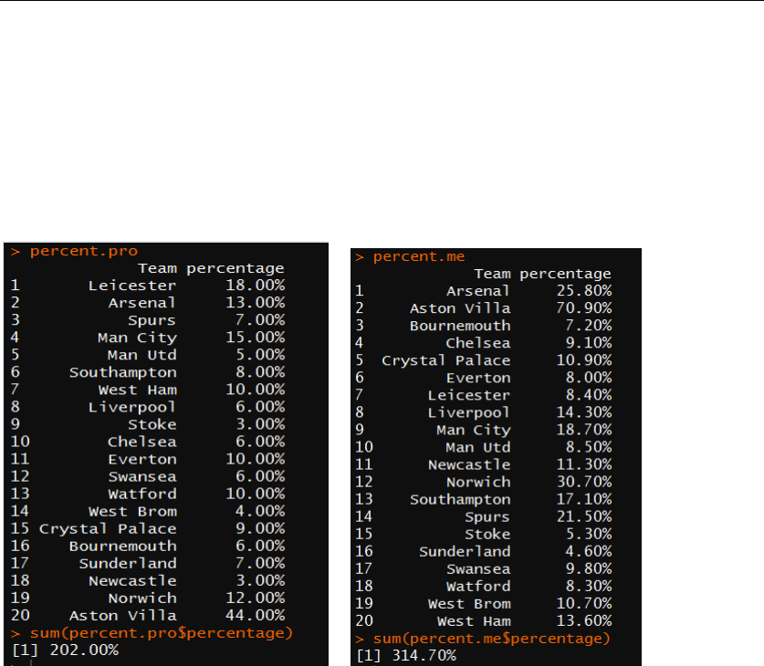
The second test is a percentage test—that is, to test the percentage of the teams

occur to be at their correct rank(i.e. the real-world rank) in the simulation. In this part,

I created a function percentage_test() to solve the problem. Moreover, I calculated the

sum of percentages of each team. The larger the summation is, the more accurate the

model performs. Test results is shown on figure 13.

Figure 13: Percentage of teams at their right place and the summation of the percentages.

Left: model 1 Right: Model 2

From the test results, I noticed that model 2 has much better accuracy on middle-

ranked teams and has an average 5.635% higher accuracy on each team than model 1,

which indicates that generally speaking model 2 performs a significantly higher

accuracy than model 1.

(3)

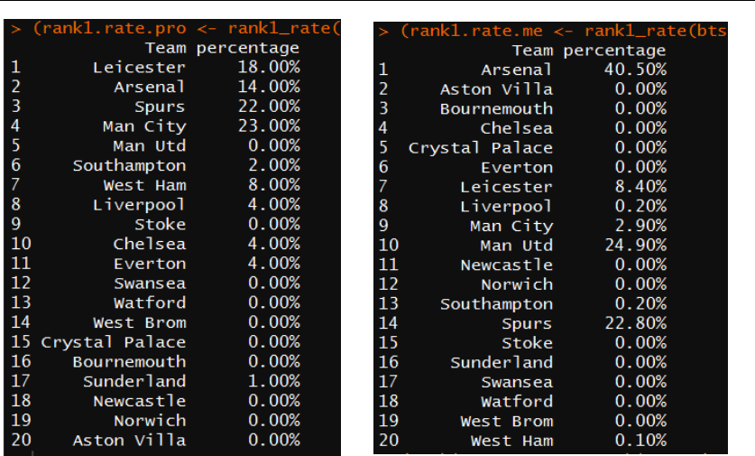
The third test that I designed is about the accuracy of simulating the champion,

which is measured by the percentage of each teams win the champion in simulated

2015-16 season. Since Leicester City was a surprising dark horse in last year, I required

my best model for predicting 2016-17 season to do its best on predicting the

championship without influence the accuracy of other ranks. To complete the test, I

wrote a function rank1_rate() and the next figure is the result of the tests:

Figure 14: Test results of the percentages of win a champion. Left: model 1 Right: model 2

From the above figure, I saw that model 1 does better in predicting the champion.

However, an interesting appearance is that in model 2, all the top 6 teams except

Leicester has extremely high percentage to win the champion while on the other side,

many middle-ranked teams and relegation avoiders still have considerable chance to

win the chance, which is ridiculous and might indicates that even though model 1

performs better in predicting the champion, it sacrifices a lot in accuracy of other ranks.

After general consideration of all 3 tests, I choose model 2 as my prediction model

in the next section.

VI. Prediction

Knowing that model 2 is the better one, now I start predict the 2016-17 Premier

League final points and team ranks. Since there were 3 teams from 2015-16 season

degraded down to the Football League Championship and 3 new teams upgraded to

Premier League, I can’t simply take the model 2 in 2015-16 season to predict the results

in 2016-17 season. Therefore, I chose to re-construct a model that based on the ideas of

model 2 in 2015-16 season.

One crucial problem occurred in this part is the estimation of Poisson parameters

of each team. Since the season is still in progress, I imported and select the completed

14 rounds of game results(last updated at 12/06/2016, total 14 rounds) as training sets

and estimate the Offence, Defence and home parameters to predict the result of rest of

games. Like what I have shown on section IV, I predicted the result of rest of games

and combined them with the finished games to produce the following predicted final

table of 2016-17 Premier League Season:

Figure 15: Top: Result table of finished 14 rounds of games(up to 12/06/2016)

Bottom: Predicted result table of 2016-17 Premier League Season using first 14-round

games data

Comparing the top and the bottom of figure 15, we can see that the top 5 teams in

the first 14 rounds stay consistent in the rest of the matches and Chelsea, who has

outstanding home results and steady away performance win the champion of 2016-17.

Tragically, the defending champion, Leicester city, performs bad in this season and

could only strive to avoid relegation. Surprisingly, Spurs who ranks 5

in first 14 rounds

seems to have huge potential in the next 24 rounds and finally win a 2

rank while

Arsenal seems to become laxity in the second half and wastes their accumulated

advantages in the first 14- rounds.

VII. Future Developments

The project might be improved in those ways:

1. Our predictors only cover those naïve ones and more possible parameters that may

have influence on the game results should be considered. For instance, the injuries

situations is neglected in this project but is actually crucial in the real world. If

haunted by a large amount of injuries, those top teams like Arsenal and Chelsea

might face a hard time even when they are playing with those less competitive teams.

Another nice example is the influence of schedule and other game events like

champions league. If Manchester United has to play against Real Madrid in the

weekdays on Champions league and has also to play against Arsenal at the weekend,

the travel fatigue and the intense schedule might make them lose the game that they

ought not to lose.

2. There might be other models that performs better than naïve Poisson regression

model. For example, Hierarchical Bayesian Poisson Model introduced by Rasmus

Baath seems to have full use of given data as prior information, and its detailed

hierarchy might lead to more accurate results. Moreover, stepwise prediction that

produces new estimation of parameters for the next step might also have a higher

prediction accuracy.

3. One possible way to improve the accuracy in the current project is to augment the

matrix and increase the data of those teams that are never relegated from the Premier

League to figure out more accuracy estimators of those teams’ parameters.

VIII. Conclusion

In this project, I discovered that the goals of each game follows Poisson distribution

and figured out the least square estimator of Poisson parameter λs for each team by

fitting the number of goals Y with a generalized linear model onto the team indicator

matrix X. Based on this, I constructed two models with several modeling techniques

and simulated the game results to obtain the predictions. Then, I designed three tests on

two models and chose the best one for the prediction after an overall consideration of

various aspects.

Within the best model, I successfully predicted the final result table of 2016-17

Premier League within the completed games. An overall observation indicates that my

predicted results have a consistent trend as the completed games, which indicates that

the result is reasonable and acceptable.

IX. References

1. Rasmus Bååth. “Modeling Match Results in Soccer using a Hierarchical Bayesian

Poisson Model”.

http://www.sumsar.net/papers/baath_2015_modeling_match_resluts_in_soccer.pdf

2. Pinnacle.com. https://www.pinnacle.com/en/betting-articles/soccer/how-to-

calculate-poisson-distribution, Aug 12, 2014

3. Premier League website. https://www.premierleague.com/

4. Github user Jargnar. https://raw.githubusercontent.com/jargnar/premier-league-

data/master/2015-16/data.csv