
Murray State's Digital Commons Murray State's Digital Commons
Honors College Theses Student Works
Spring 4-25-2024
Examination of the Top 10 Stocks in the S&P500 Examination of the Top 10 Stocks in the S&P500
Isaac Fulton
Follow this and additional works at: https://digitalcommons.murraystate.edu/honorstheses
Part of the Finance and Financial Management Commons
Recommended Citation Recommended Citation
Fulton, Isaac, "Examination of the Top 10 Stocks in the S&P500" (2024).
Honors College Theses
. 241.
https://digitalcommons.murraystate.edu/honorstheses/241
This Thesis is brought to you for free and open access by the Student Works at Murray State's Digital Commons. It
has been accepted for inclusion in Honors College Theses by an authorized administrator of Murray State's Digital
Commons. For more information, please contact [email protected].
Murray State University Honors College
HONORS THESIS
Cercate of Approval
Examinaon of the Top 10 Stocks in the S&P500
Isaac Fulton
April/2024
Approved to fulll the _____________________________
requirements of HON 437 Dr. David Durr
Finance
Approved to fulll the _____________________________
Honors Thesis requirement Dr. Warren Edminster, Execuve Director
of the Murray State Honors Diploma Honors College

Examinaon Approval Page
Author: Isaac Fulton
Project Title: Examinaon of the top 10 stocks in the S&P500 in relaon to the overall porolio
Department: Finance
Date of Defense: 4/25/2024
Approval by Examining Commiee:
________________________________________ ____________________
(Dr. David Durr, Advisor) (Date)
________________________________________ _____________________
(Professor Chistopher Wooldridge, Commiee Member) (Date)
________________________________________ ______________________
(Dr. Leiza Nochebuena-Evans, Commiee Member) (Date)
Examinaon of the Top 10 Stocks in the S&P500
Submied in paral fulllment
of the requirements
for the Murray State University Honors Diploma
Isaac Fulton
April / 2024
i
Abstract
The major goal of this research was to invesgate how the returns of a porolio
containing only the 10 largest stocks in the S&P500 index, based on market cap, would compare
to the overall index’s return and volality over mulple me frames. This project invesgated
whether a porolio of the 10 largest stocks in the S&P500, at the beginning of each year, would
be considered superior in terms of returns while not unproporonately increasing volality.
First, the SPDR S&P 500 ETF Trust, or SPY, was selected as the S&P500 index measure and was
used to evaluate the index’s returns. Second, the largest stocks in the index for each year
between 2016 and 2022 were selected and each of their market capitalizaons at the beginning
of that year were measured as a percentage of the total index’s. Returns for each stock, for each
month, were then sourced from a database provided by faculty at Murray State. Two dierent
test porolios were then generated containing the largest 10 stocks for each year, only diering
on how the ten largest stocks were weighed. Finally, the Invesco S&P 500 Top 50 ETF (XLG)’s
returns were also calculated to determine how a porolio containing the 50 largest stocks in the
index would perform compared to the index and the test porolios. Since the XLG is comprised
of only the 50 largest stocks in the S&P500, it may give us a good measure of how powerful the
ten largest stocks are, even in comparison to the other 40 largest rms. Once all the returns of
the four porolios had been collected, the index and test porolios’ return, betas, and standard
deviaons were calculated and compared to nd results. Aer comparing the test porolios
with the SPY, what was discovered was that during 2016 through 2022 a porolio containing the
10 largest stocks in the S&P500, as measured at the beginning of each year and weighed in
accordance with each stock’s index weight, would produce the best possible returns of any
ii
porolio analyzed, but would increase the porolio’s standard deviaon and beta. Aer running
a risk-adjusted analysis, what ulmately was discovered was that while the porolios containing
only the largest stocks did experience larger returns during the 7 years, that on a total risk-
adjusted basis, they produced less returns per unit of risk taken. This was concluded to be
because of the porolios’ lack of diversicaon, which no maer its larger returns, could not
outperform that of the market when accounng for its volality. Finally, to demonstrate that
there are sll benets to these types of porolios and the increased returns they can generate, I
ran a new scenario analysis, ending the study aer 2021.
iii
Table of Contents
Abstract………………………………………………………………………………………………………….….…i
Table of Contents……………………………………………………………………………………………..…..iii
List of Figures and Tables……………………………………………………………………………….……….iv
Introducon …………………………………………………………………………………………………………1
Goals of Research……………………………………………………………………………………………….…4
S&P500 Stock Weighng…………………………………………………………………………………………4
Analysis Methodology………………………………………………………………………………………..…..6
Test Porolios – Equally weighted and Index weighted…………………………………………………7
Market Players – Test Porolios Composion…………………………………………….…...10
Rebalancing the Porolios……………………………………………………………………….….12
Individual Stock Analysis………………………………………………………………………….…13
Monthly Return Comparison………………………………………………………………………………….15
Total Return Comparison………………………………………………………………………………………17
Yearly Return Comparison…………………………………………………………………………………….18
Standard Deviaon Comparison – Yearly and Monthly Basis……………………………………….19
Beta…………………………………………………………………………………………………………………..22
Invesng Scenarios……………………………………………………………………………………………...23
Analysis Limitaons……………………………………………………………………………………………..26
Risk-Adjusted Comparison………………………………………………………………………………......26
Sharpe……………………………………………………………………………………………………..27
Drawbacks of Sharpe Measure………………………………………………………………….….29
Treynor’s Measure………………………………………………………………………………….…..30
Jenson’s Alpha…………………………………………………………………………………….…….32
Risk-Adjusted Comparison Summary…………………………………………………….….….35
Alternave Analysis: What if the analysis ended aer 2021?............................................35
Research Findings Summary………………………………………………………………………………….37
References………………………………………………………………………………………………………….41
iv
List of Figures and Tables
Figure 1- Invesng $1000 into the S&P500 in 2000 and leaving unl 2023 ……………………….3
Figure 2- S&P 500 monthly returns (2000-2023)………………………………………………………….4
Figure 3 – Percentage of total Index market cap residing in the Largest 10 stocks in the S&P500
as of January 1st, 2024…………………………………………………………………………….….6
Figure 4 – Largest 10 stocks in the S&P500 and their index weights at the beginning of each year
between 2016 and 2022………………………………………………………………………………….11
Figure 5 – Ten largest Stocks’ names, rankings, weights per test porolio, betas, and standard
deviaons of monthly returns from 2016 through 2022…………………………………15
Figure 6 – Number of Months the test porolios out/underperformed the SPY from 2016-
2022…………………………………………………………………………………………………………………..16
Figure 7 – Correlaon of our test porolios’ Monthly Returns to that of the SPY………………16
Figure 8 – Porolio Total Returns from 2016 through 2022…………………………………………..17
Figure – 9 Porolio’s yearly returns.…………………………………………………………………………18
Figure 10 – Comparison of Porolio Standard deviaon…………………………………………..…20
Figure 11 – Porolio Monthly return standard deviaon for each year in study……………..…20
Figure 12 – Porolio Beta of each year – using Monthly returns for each year (2016-2022)..22
Figure 13 – Porolio Beta of enre period – Using Monthly Returns for enre period (2016-
2022)………………………………………………………………………………………………………………….22
Figure 14 – Porolio Beta of enre period – Using yearly Returns for enre period (2016-
2022)…………………………………………………………………………………………………………………22
Figure 15 – Risk-Adjusted Rao Analysis Summary……………………………………………………27
Figure 16– Sharpe and Treynor Measure Component Informaon………………………………..30
Figure 17 – Treynor Measure Component Informaon………………………………………………..31
Figure 18– The SML on investments invested from 2016 through 2022………………………….34
Figure 19 – Porolios’ Yearly Compounded Returns from 2016-2022…………………………...36
Figure 20 – Alternave Analysis – Risk-Adjusted Analysis Summary…………………………..…37
Figure 21 – The SML on investments invested from 2016 through 2021…………………………37
1
Introducon
The S&P500 is one of the best-known equity indexes in the enre world and is
comprised of the ve-hundred largest companies traded on either the NYSE, Nasdaq, or CBOE.
The porolio technically includes over 500 separate stocks, as 3 of these companies have
mulple classes of stock, resulng in 503 tradable stocks in the index. The Index had a market
capitalizaon, as of January 1
st
, 2024, of over 40 trillion dollars, which comprises 80% of total US
business’s market capitalizaon. The S&P500 is preferred for instuonal investors over its
competors, such as the DOW JONEs index (Yahoo Finance, 2024), because of its inclusion of
more stocks across dierent sectors, and therefore is considered to be a more accurate
representaon of the US’s equies market (KENTON, 2023). The S&P500 index’s construcon
seeks to include stocks from all industries in an aempt to mimic how the overall economy is
moving. Through including many stocks from every sector, the index is thought to diversify out
unsystemac risk. This is why many investors use the S&P500 as a benchmark for the market
and many ETFs and Index funds have been created to mirror the composion of the index.
Currently, there are many ETFs and index funds that track the S&P500, all with their
slightly dierent goals. The oldest and most popular ETF mirroring the S&P500, was created in
1993 and is named the SPDR S&P 500 ETF Trust (SPY). SPY is a passively managed fund run by
State Street, with a goal of mirroring the S&P500. Another ETF tracking the S&P500, is the
Invesco S&P 500 Top 50 ETF (XLG), which only includes the 50 largest companies in the S&P500
and was created in 2005. Because both funds are passively managed, this means that both aim
to replicate the performance of the underlying index as closely as possible. Both ETFs oer
2
unique ways to compare porolios to the market and for this reason, I used both these ETFs as
market measures to compare my research’s porolios return and volality against.
Aside from ETFs, the three largest S&P500 index funds currently are the Fidelity 500
index fund, Schwab S&P 500 index fund, and the Vanguard 500 Index Admiral Fund (Reeves,
2024). While index funds and ETFs are very similar, they do have some dierences that can
result in dierent returns for the porolio. Index funds are generally considered safer than ETFs,
but they cannot be traded during the day and cannot be bought and sold on exchanges like
ETFs. This allows Index funds to provide more stable, long-term investment avenues, as they
primarily trade in securies via asset management companies and are therefore great for
paent investors. ETFs on the other hand oer more exibility, lower costs, and higher tax
eciency than Index funds, but are also more volale and garner more trading fees. While both
ETFs and index funds seek to match the performance of the market, ETFs have proven to be
beer for short-term investors and Index funds have shown to be beer for long-term investors.
Because this analysis only invesgates 7 years’ worth of data, and hence will be looking at a
relavely small-me frame, it will ulize both the SPY and XLG ETFs’ returns and volality to
compare to that of my test porolios.
Overall, the S&P500 is viewed as a safe investment by most analysts as it has
experienced a consistent history of long-term growth. In fact, if you invested $1000 in a
porolio mirroring the S&P500 index in 2000, by the end of 2023 you’d have $4,880.49, a return
of 388.05%, or 6.93% per year (Webster, 2024). A graphical depicon of this investment can be
seen in gure 1. Adjusng for inaon this would give the investor a 175.82% return over the 23
years. While the market does go through bull and bear markets, the S&P500 has proven over its
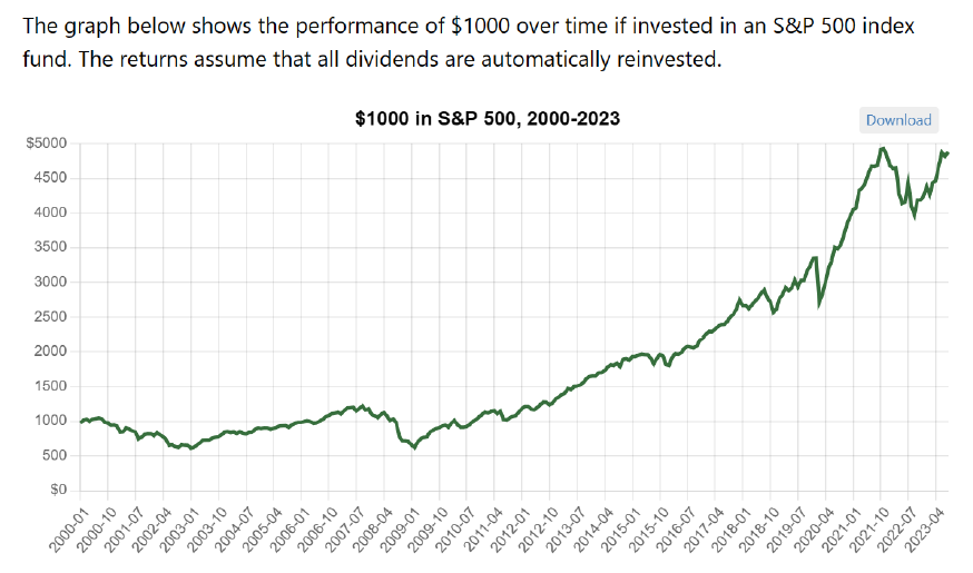
3
history that it will connue to grow and produce posive results in the long term. A graphic
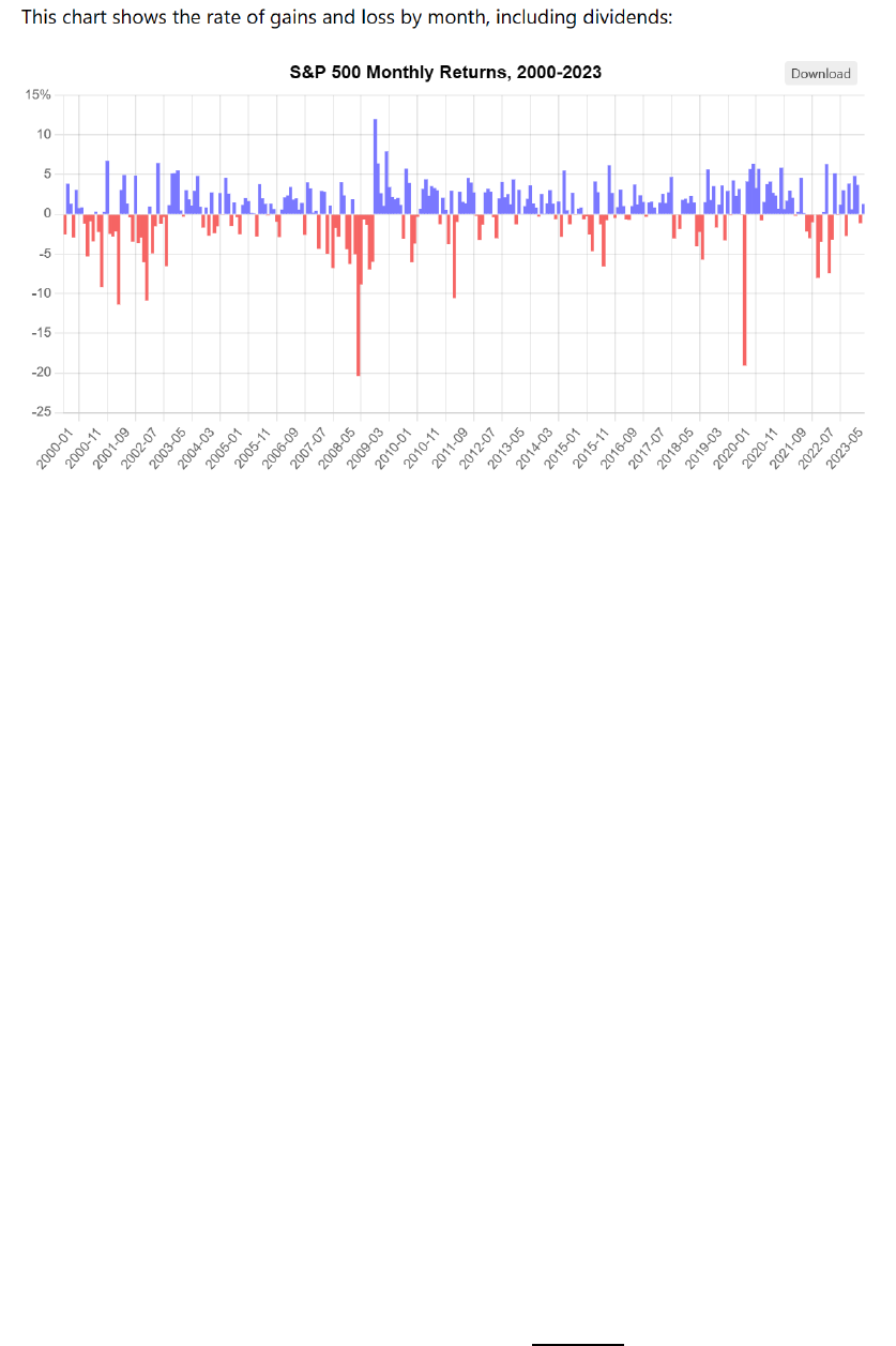
depicon of the S&P500’s returns from 2000 to 2023 can be seen in gure 2. As we can see in
gure 2, while there have been plenty of negave months in terms of returns, they are
outnumbered by the posive returns that the index has generated. This history of long-term
growth is one of the reasons the S&P500 has become so popular as a measure of the market
and is why I used its measure as the benchmark for this analysis.
Figure 1- Invesng $1000 into the S&P500 in 2000 and leaving unl 2023. From Ocial Data, 2024., Retrieved from
hps://www.ocialdata.org/us/stocks/s-p-500/2000?amount=1000&endYear=2023. Copyright 2024 by Ian Webster.
4
Figure 2- S&P 500 monthly returns (2000-2023). From Slick Charts, 2024., Retrieved from
hps://www.slickcharts.com/sp500/returns. Copyright 2024 by Slick Charts.
Goals of Research
The goal of this paper ulmately is to discover whether a porolio containing the ten
largest stocks in the S&P500 index could potenally outperform the market, as measured by the
SPY, in terms of total returns as well as on a risk-adjusted basis. Addionally, a secondary goal of
this paper will be to get a sense of how much the ten largest stocks of any given year aect the
overall return and volality of the index. Through analyzing the SPY, I will seek to measure the
ten largest stocks impact on the overall market, and by analyzing the XLG, I will seek to view the
ten largest stocks impact compared to that of only the 50 largest stocks.
S&P500 Stock Weighng
The S&P500 index weighs its stocks based on their percentage of total market
capitalizaon, and therefore those stocks with more weight can aect the price more
dramacally. Recently, a real-life example of this would be Microso which, as of March 12
th
,

5
2024, was the largest stock in the S&P500 with an index weight of 6.98%. V.F. Corporaon as of
March 12
th
was the smallest stock in the S&P500 with an index weight of .01%. This meant that
at that me Microso, the largest stock, had 698 mes the weight of the smallest stock in the
index, demonstrang the sheer power that the largest stocks have in the index. Now while
obviously the largest stock might be much greater than the smallest stock, how would it
compare to the median stock, the 250
th
largest stock in the index? In this case, Electronic Arts
(EA), the 250th largest stock as of March 12
th
, had an index weight of .08%. Therefore, in this
case, Microso would sll possess 87.5 mes the weight of EA, demonstrang that this one
stock controls much more of the total return of the index than the enre boom half of the
index.
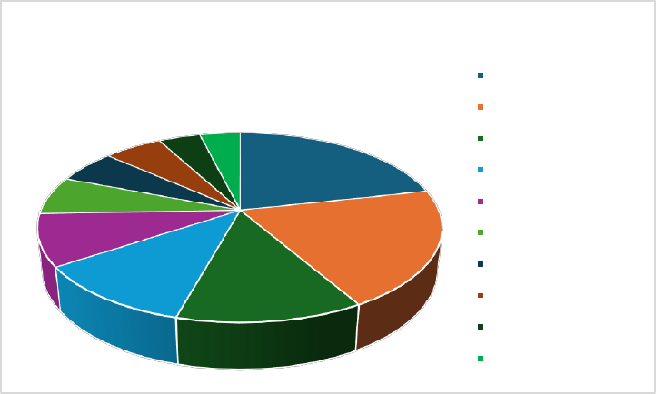
Through this paper’s analysis it was discovered that the S&P500 index is very top heavy,
as its largest 10 stocks in any given year between 2015 and 2023 accounted for, on average, 26%
of the total index’s market cap. This 26% is also not telling of the whole story either, as the top
ten stocks percentage increased throughout the 7-year period, with every year aer 2020
having a larger percentage than 26%. Figure 3 below depicts just this, as it shows the rankings of
the 10 largest stocks in the S&P500 as of January 1
st
, 2024, with these stocks collecvely holding
34.7% of the whole market cap of the index. This disparity between the top stocks in the index
can be seen even clearer when I also included the top 11-20 stocks. Between 2015 and the end
of 2023, on average, 36.9% of the index’s market cap resided within its top 20 stocks, with a
similar increasing percentage trend as seen with the top 10 stocks. This concentraon at the top
of the index leaves the remaining 480 or so stocks to have on average .13% of the index’s
market capitalizaon per stock. This disparity at the top is what led me to our queson in this
6
paper; would invesng in a porolio of only the top 10 largest stocks in the S&P500, over a
mul-year period, produce superior returns while not unproporonally increasing risk and
volality? Many believe that to achieve the best returns, a porolio or index must be well
diversied, but with the power that resides in the ten largest stocks of the S&P500, there is
room to queson whether that remains true.
Figure 3 – Percentage of total Index market cap residing in the Largest 10 stocks in the S&P500 as of January 1
st
, 2024.
Analysis Methodology
The 10 and even 20 largest stocks of the S&P500 index represent a massive poron of
the overall index’s market capitalizaon. To invesgate whether it is sll true that the other 490
or so stocks are sll necessary to diversify risk in a porolio and return the best possible returns,
an analysis and comparison of the returns of the top 10 stocks in the S&P500 over a 7-year
period was conducted.
The Ten Largest Stocks' Percentage of the Total
Index's Market Cap
34.7%
Apple
Microsoft
Alphabet
Amazon
NVIDIA
Meta/Facebook
Tesla
Berkshire Hathaway
Eli Lilly
Visa
7
To begin this analysis, rst the largest 10 stocks at the beginning of each year between
2016 and 2022 were ranked by their total market capitalizaon. Then the overall S&P500 index’s
market capitalizaon was found for each of these years. To test the performance of solely the
largest ten stocks in the index, two test porolios were created and compared to the index over
the 7 years. Aer the returns for each month, year, and total period were calculated for the test
porolios and SPY, each porolio’s beta and standard deviaon was calculated for the same
periods. To see how returns can dier depending on frequency, mulple invesng scenarios
were then examined to see how invesng $1000 in each porolio could dier over the 7-year
me in regards to compounding. Aer the returns and volality of the test porolios were
analyzed, a risk-adjusted review was completed, to determine whether these porolios could
outperform the market without increasing risk unproporonately. The results of the analysis are
shown in the following secons and gures in this paper.
Test Porolios – Equally weighted and Index weighted
To evaluate the eect of the ten largest stocks on the total return of the S&P500, this
analysis used two dierent test porolios comprised of the largest 10 stocks as of the beginning
of each year. The two test porolios were comprised of the same stocks each year and diered
only based upon how these stocks were weighed in the porolio. The rst test porolio equally
weighed each of the 10 largest stocks of the S&P500 each year, and therefore each stock’s
performance inuenced the porolio’s total return equally. The second test porolio weighed
each stock relave to its weight in the index. This second porolio allowed for the very largest
stocks to inuence the total porolio’s returns and volality more than the 9
th
or 10
th
largest
stocks and more accurately reects the power that each stock has in the index.
8
We will invesgate the results of both test porolios because each weighng method
brings its own benets and drawbacks to the analysis. To begin, the benets of the equally
weighted test porolio are that it removes the large cap bias of the index and returns results
that reect every stock’s performance equally. Market-cap weighted porolios on the other
hand, are overweight in companies that are currently outperforming the market and thus they
allow themselves to have a large concentraon of funds at the top of the porolio. Because of
this concentraon in overvalued stocks, market-cap weighted porolios are great for when the
largest companies are on a tear, but over the long-term, these porolios can be massively hurt
when the overpriced stocks inevitably fall back to their fair value. Therefore, market-cap
weighted porolios have long been viewed as a great tool for momentum invesng strategies,
as during good mes they can outperform the market, yet during contracons are oen le
desolated. Oppositely, Equal Weighted porolios are more resistant to drop os like these,
because of their beer diversicaon due to less concentraon in any one stock. Equally
weighted porolios are considered value-based invesng strategies, which means that this
approach favors undervalued stocks with the potenal to rise in price and return to their fair
value. A downside to this style of invesng, however, is that it will lead to more selling and
buying acvies and potenally larger tax consequences than a market-cap weighted porolio.
For example, when shares in Company A grow and become more highly valued, a poron will
have to be sold and deployed into the lower-priced Company B, C, and D to maintain the equal
weighng of all companies in the porolio. Therefore, while the equally weighted porolio may
have greater diversicaon and focus on the true value of the stocks, it too has its downsides,
as its higher management fees can eat into its returns. Ulmately then, the type of weight used
9
in porolios depends on the goals of the investor as each method can produce superior returns
and risk depending on investment strategy.
Because of the dierences in porolios and invesng strategies, this study will ulize
both equally and market-cap weighted porolios to determine which would have performed the
best from 2016-2022. Even though equally weighted porolios tend to require more
rebalancing, and therefore can generate larger fees, there is a generally accepted view that they
sll produce superior returns and risk to that of market-cap weighted porolios (Friedberg,
2018). While this may be held as true by many investors, this paper will seek to see if this
statement would hold true between 2016 and 2022, when the market was experiencing mainly
posive years. As a control for this research, the SPY was used as the benchmark for which I will
compare both porolios returns and volality to that of the market. The XLG will also be
compared to the test porolios and the market, to see how a porolio containing only the 50
largest stocks in the index would compare.
To begin the analysis, each of the largest stocks in the SPY, as of January 1st of each year,
were selected and weighed in accordance with their test porolio. Because the largest stocks in
the index changed market capitalizaon and therefore index weight throughout the 7-year
period, each year the manager would need to rebalance the porolio, removing companies who
had shrunk, and replacing them with the new largest companies. Once the ten largest
companies had been selected for each year in the study, each stocks’ monthly returns for that
year were collected, and the porolio’s monthly returns were then calculated based on the test
porolio’s stock weights. The SPY and XLG’s monthly returns for each year during the study
were then also calculated using data from Yahoo Finance. Once each porolios’ monthly returns
10
for the enre period were calculated, each year’s twelve-monthly returns were annualized to
nd the year’s total return. Likewise, once each year’s monthly returns were calculated using
the proper stocks and weights, the total 7 year holding period return was calculated.
A fault with the returns found using this method is that it does not include the
processing fees that would be incurred to rebalance each of the test porolios each year. What
this ulmately means is that less money would be invested each year as compared to my
calculaons, as some principal would be lost to these fees. These fees would not be apparent in
investments in the SPY, as it is a market-cap weighted ETF that would be fully passively invested
in. The SPY would only require fees when the money is ulmately pulled out at the end of the
period to realize a return. These calculaons also do not account for the equally weighted
porolios larger management fees in order to keep the porolio equal and therefore may not
accurately represent the dierence between equally weighted and market-cap weighted
porolios. Therefore, while these calculaons can oer insight into how these investments
could compare to the index, their returns may be slightly inated.
Market Players – Test Porolios Composion
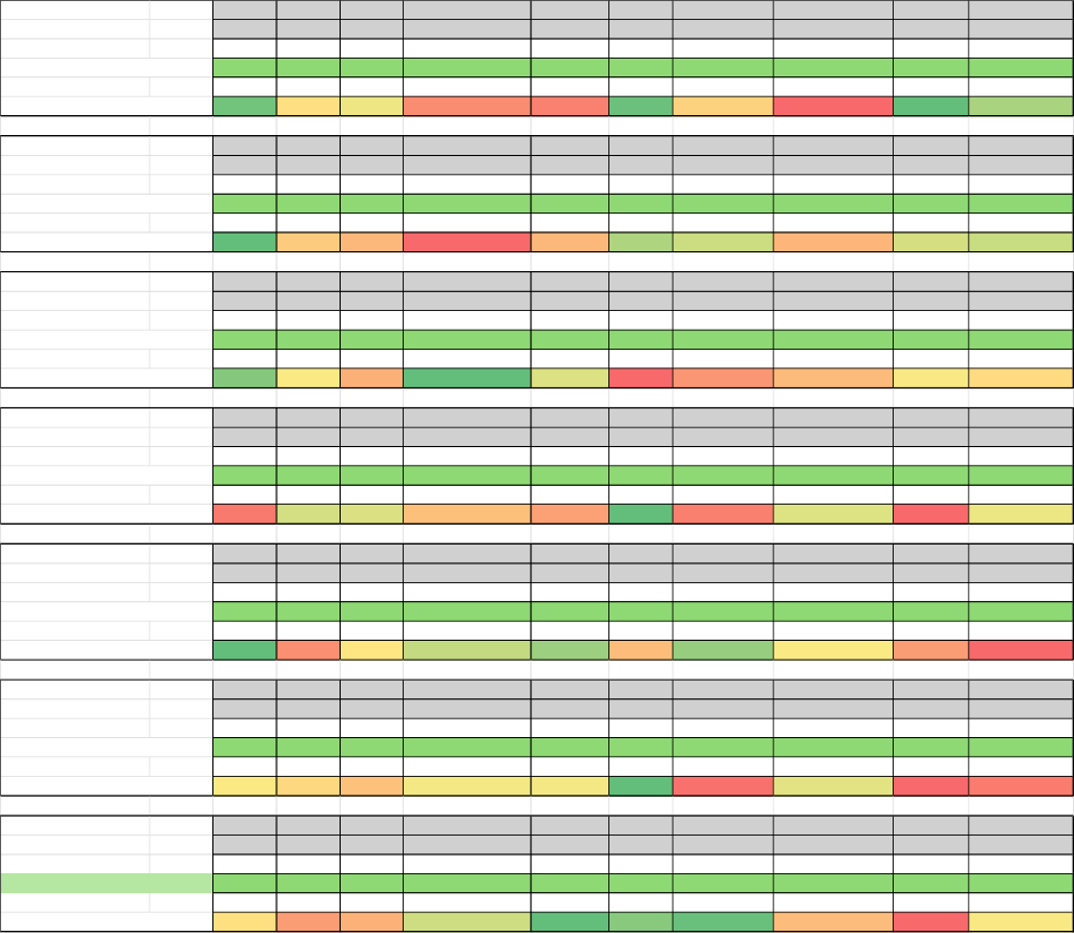
When looking at the largest stocks throughout these seven years, it is apparent who the
largest players in the market have been. Apple has been the largest company almost every year
since 2016, only being usurped by Microso at the beginning of 2019. Between 2016 and 2019
Apple consistently comprised the largest weight of the index at approximately 3.5% of the
enre index’s market capitalizaon. However, starng in 2020, the company’s market
capitalizaon began to increase to around 7% of the total index weight. Unl the end of 2019,

11
no stock had been over 4% of the total index weight, but during 2020, the disparity between the
largest companies in the index and the smallest began to grow. By the beginning of 2022, four
dierent stocks had individual index weights greater than 4%, with Apple reaching its peak
index weight of 7.19%. Another notable trend during these 7 years is that many of the largest
stocks in the index stayed consistent. Stocks such as Apple, Microso, Alphabet, and Amazon
were among the ten largest every year during the study. While the largest ve stocks were
almost always the same, albeit shued, the sixth through tenth largest stocks in the index
would occasionally dier in composion. The largest stocks and their percentage of the total
Index market capitalizaon for 2016 through 2022 can be seen in gure 4 below.
Market Cap
Rank:
2022
% of
Total
S&P
2021
% of
Total
S&P
2020
% of
Total
S&P
2019
% of
Total
S&P
2018
% of
Total
S&P
2017
% of
Total
S&P
1/1/2016
% of
Total
S&P
1
Apple
7.19%
Apple
7.05%
Apple
4.81%
Microso
3.71%
Apple
3.77%
Apple
3.16%
Apple
3.26%
2
Microsoft
6.25%
Microsoft
5.30%
Microso
4.48%
Apple
3.55%
Alphabet
3.21%
Alphabet
2.83%
Alphabet
2.99%
3
Alphabet
4.75%
Amazon
5.17%
Alphabet
3.45%
Amazon
3.51%
Microso
2.89%
Microso
2.51%
Microso
2.46%
4
Amazon
4.20%
Alphabet
3.74%
Amazon
3.44%
Alphabet
3.46%
Amazon
2.47%
Berkshire
Hathaway
2.09%
Berkshire Hathaway
1.82%
5
Tesla
2.71%
Meta/Facebook
2.46%
Meta/Facebook
2.19%
Berkshire
Hathaway
2.39%
Meta/Facebook
2.25%
Exxon Mobil
1.94%
Exxon Mobil
1.81%
6
Meta/Facebook
2.28%
Tesla
2.14%
Berkshire Hathaway
2.06%
Meta/Facebook
1.78%
Berkshire
Hathaway
2.14%
Amazon
1.85%
Amazon
1.78%
7
NVIDIA
1.82%
Berkshire
Hathaway
1.70%
JPMorgan Chase
1.61%
Johnson &
Johnson
1.63%
Johnson & Johnson
1.64%
Meta/Facebook
1.72%
Meta/Facebook
1.66%
8
Berkshire Hathaway
1.64%
Visa
1.50%
Visa
1.53%
JPMorgan Chase
1.52%
JPMorgan Chase
1.63%
Johnson & Johnson
1.63%
Johnson & Johnson
1.59%
9
United Health
1.17%
Johnson & Johnson
1.31%
Johnson & Johnson
1.43%
Visa
1.40%
Exxon Mobil
1.55%
JPMorgan Chase
1.60%
Wells Fargo
1.55%
10
JPMorgan Chase
1.16%
Walmart
1.29%
Walmart
1.26%
Exxon Mobil
1.37%
Bank of America
1.35%
Wells Fargo
1.44%
JPMorgan Chase
1.35%
Figure 4 – Largest 10 stocks in the S&P500 and their index weights at the beginning of each year between 2016 and 2022.
Informaon was adapted from “Top 20 S&P 500 Companies by Market Cap (1990 – 2024)” (FINHACKER, 2024)
Rebalancing the Porolios
12
As can be seen in gure 4, each year the largest stocks in the SPY change and their
weight moves in accordance with their companies’ new market capitalizaon. Depending on
invesng schedule, even if funds invested in each of these test porolios were le for the enre
7-year period, the largest stocks in the SPY would change each year and would result in the
porolios needing to be rebalanced. Each year, the manager would calculate the largest ten
stocks in the SPY and then appropriately weigh the stocks based on the test porolio. For this
analysis, these calculated monthly returns of the SPY, XLG, and test porolios were used to
calculate the annualized yearly and 7-year returns.
The Ecient Market Hypothesis (EMH) demonstrates that no acve manager can beat
the market for long, as their success is only a maer of chance. Therefore, longer-term, passive
management has proven to deliver beer returns overme. My inial quesons for this paper
then were: how would a hybrid strategy perform where stocks are acvely selected and
rebalanced, but funds are le passively to grow? I try to answer this queson below, as well as:
would the ten largest stocks of the index, if acvely managed and rebalanced once a year,
provide superior returns without increasing the risk of the porolio unproporonately to that of
the index? The following secons of this paper seek to invesgate whether the two test
porolios would provide superior returns and measures of volality as compared to the market
between 2016 and 2022. The next part then seeks to compare the test porolios to the market
on a risk-adjusted basis.
Individual Stock Analysis
13
Throughout the 7-year period under analysis, the 10 largest stocks in the index remained
relavely stable. There were 6 dierent stocks who maintained top 10 status throughout the
enre period, with 13 dierent stocks in total being included at some point in the test
porolios. Each of these stocks played a role in determining the return and volality of the test
porolios as well as the SPY and XLG. To discover where volality came from during these years
under invesgaon, the standard deviaon, beta, and average stock rank were calculated for
each stock. A summary of the individual analysis of each company included in the index can be
found in gure 5.
As can be seen in gure 5, Apple was the largest company for all but one year of the
study. This means that throughout my analysis, Apple was the main driver of returns and
volality for all the porolios under analysis, except the equally weighted porolio. In fact, aer
analyzing the stocks who were included in my test porolios, 4 specic stocks, which were
present every year, stood out as drivers of returns and volality. These were, unsurprisingly,
Apple, Microso, Alphabet, and Amazon. These four stocks consistently ranked within the
largest 4 throughout the period and none of them even dropped below the 6
th
largest posion.
While these stocks were found to be the largest throughout the period, they were also found to
have experienced the largest standard deviaon during their me in the test porolios. This
leads to the idea that while the very largest stocks are responsible for generang the majority of
returns for even a porolio containing only the largest 10 stocks, they are also responsible for
generang the majority of volality for that porolio. In fact, every stock that ranked within the
10 largest every year of the study (7 mes) had a standard deviaon larger than that of the test
porolios. This means that while the largest returns of the test porolios are generated by the
14
largest stocks, the risk reducon of the test porolios comes from the boom half of the
porolio.
Another interesng thing discovered about these largest stocks was that, except for two
instances at the beginning of the study, the majority of stocks experienced betas of over 1.
Having a beta above 1 means these stocks are more volale and therefore riskier than the
market. What this ulmately means is that when the market reacts to changes, these stocks on
a whole will react more drascally than the market. This can be good for years when the market
is performing well, but as we can see when calculang yearly returns, when the market goes
south, the test porolios take even larger nose dives.
15
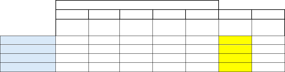
Figure 5 – Ten largest Stocks’ names, rankings, weights per test porolio, betas, and standard deviaons of monthly returns from
2016 through 2022.
Monthly Return Comparison
To perform my monthly return analysis, the returns of each of the ten largest stocks in
the SPY were calculated, for each month of the 7 years. Each stock’s monthly return would be
weighted according to the test porolio to calculate the porolios’ total return for each month.
To calculate the returns of the XLG and SPY, their historical prices were sourced from Yahoo
Finance, and the holding period formula was used to calculate their monthly returns.
Stock Size 1 2 3 4 5 6 7 8 9 10
Top 10 as of 1/1/16 Apple Alphabet Microsoft Berkshire Hathaway Exxon Mobil Amazon Meta/Facebook Johnson & Johnson Wells Fargo JPMorgan Chase
Equal Weight Portfolio
10% 10% 10% 10% 10% 10% 10% 10% 10% 10%
Index Weighted Portfolio
16.10% 14.75% 12.13% 8.98% 8.94% 8.78% 8.18% 7.84% 7.64% 6.67%
Stock Beta
1.54 1.04 1.10
0.67 0.29
1.50
-0.03 0.09
1.48 1.59
Standard Deviation (Monthly Ret)
7.52% 5.63% 6.06% 4.03% 3.80% 7.61% 5.36% 3.33% 7.70% 6.86%
Stock Size 1 2 3 4 5 6 7 8 9 10
Top 10 as of 1/1/17 Apple Alphabet Microsoft Berkshire Hathaway Exxon Mobil Amazon Meta/Facebook Johnson & Johnson
JPMorgan Chase
Wells Fargo
Equal Weight Portfolio
10% 10% 10% 10% 10% 10% 10% 10% 10% 10%
Index Weighted Portfolio
15.22% 13.65% 12.07% 10.04% 9.35% 8.90% 8.29% 7.83% 7.72% 6.92%
Stock Beta
1.90 1.02
0.61 0.88 -0.32
1.85 1.13
0.95 0.91 0.30
Standard Deviation (Monthly Ret)
6.16% 3.73% 3.42% 2.10% 3.41% 5.25% 4.89% 3.38% 4.77% 4.92%
Stock Size 1 2 3 4 5 6 7 8 9 10
Top 10 as of 1/1/18 Apple Alphabet Microsoft Amazon
Meta/Facebook
Berkshire Hathaway
Johnson & Johnson
JPMorgan Chase Exxon Mobil Bank of America
Equal Weight Portfolio
10% 10% 10% 10% 10% 10% 10% 10% 10% 10%
Index Weighted Portfolio
16.47% 14.00% 12.63% 10.78% 9.81% 9.36% 7.18% 7.10% 6.78% 5.89%
Stock Beta 0.83
1.25 1.25 2.12
0.75 0.93 0.73
1.06 1.14 1.17
Standard Deviation (Monthly Ret)
10.21% 6.62% 5.81% 11.25% 7.56% 5.00% 5.52% 5.93% 6.69% 6.28%
Stock Size 1 2 3 4 5 6 7 8 9 10
Top 10 as of 1/1/19 Microsoft Apple Amazon Alphabet
Berkshire Hathaway
Meta/Facebook
Johnson & Johnson
JPMorgan Chase Visa Exxon Mobil
Equal Weight Portfolio
10% 10% 10% 10% 10% 10% 10% 10% 10% 10%
Index Weighted Portfolio
15.26% 14.59% 14.42% 14.21% 9.83% 7.32% 6.72% 6.25% 5.75% 5.65%
Stock Beta 0.77
1.35 1.37
0.69 0.90
2.14
0.73
1.28
0.49
1.30
Standard Deviation (Monthly Ret)
4.12% 6.80% 6.58% 5.04% 4.63% 9.87% 4.20% 6.52% 3.91% 6.12%
Stock Size 1 2 3 4 5 6 7 8 9 10
Top 10 as of 1/1/20 Apple Microsoft Alphabet Amazon
Meta/Facebook
Berkshire Hathaway
JPMorgan ChaseVisa
Johnson & Johnson
Walmart
Equal Weight Portfolio
10% 10% 10% 10% 10% 10% 10% 10% 10% 10%
Index Weighted Portfolio
18.33% 17.07% 13.12% 13.09% 8.33% 7.86% 6.12% 5.83% 5.46% 4.80%
Stock Beta
1.23
0.64 0.98 0.83
1.22
0.88
1.24 1.05
0.71 0.35
Standard Deviation (Monthly Ret)
11.48% 6.73% 8.99% 10.01% 10.62% 7.92% 10.72% 9.19% 7.08% 5.75%
Stock Size 1 2 3 4 5 6 7 8 9 10
Top 10 as of 1/1/21 Apple Microsoft Amazon Alphabet
Meta/Facebook
Tesla
Berkshire Hathaway
Visa
Johnson & Johnson
Walmart
Equal Weight Portfolio
10% 10% 10% 10% 10% 10% 10% 10% 10% 10%
Index Weighted Portfolio
22.28% 16.75% 16.35% 11.81% 7.77% 6.76% 5.36% 4.73% 4.13% 4.07%
Stock Beta 0.84
1.39
0.71
1.65 1.19 1.36 1.03
0.99 0.62
1.08
Standard Deviation (Monthly Ret)
6.50% 6.01% 5.71% 6.92% 6.91% 14.96% 4.64% 7.83% 4.52% 4.78%
Stock Size 1 2 3 4 5 6 7 8 9 10
Top 10 as of 1/1/22 Apple Microsoft Alphabet Amazon Tesla
Meta/Facebook
NVIDIA
Berkshire Hathaway
United Health
JPMorgan Chase
Equal Weight Portfolio
10% 10% 10% 10% 10% 10% 10% 10% 10% 10%
Index Weighted Portfolio
21.67% 18.84% 14.32% 12.67% 8.16% 6.89% 5.49% 4.95% 3.53% 3.48%
Stock Beta
1.21
0.90 0.93
1.25 1.37
0.51
2.46 1.01
0.44
1.21
Standard Deviation (Monthly Ret)
9.50% 6.95% 7.72% 12.63% 18.39% 16.38% 18.14% 8.13% 4.94% 10.34%
16
When analyzing the four porolios’ returns, I began by comparing them on a monthly
basis. To do this, I started by lisng each porolio’s monthly returns for the enre 84-month
period. Then, each of the test porolio’s returns, as well as the XLG’s, were subtracted from the
SPY’s to see which performed beer during each month. Of the 84-month period analyzed, the
index weighted porolio outperformed the index 50 mes, which was far more than it lagged
behind. The equally weighted porolio performed similarly, outperforming the Index 48 mes.
Interesngly, the XLG, comprised of the 50 largest stocks in the SPY, outperformed the index the
exact same number of months as it underperformed it. The results of this analysis are shown
below in gure 6.
Equal
Index W
XLG
Months Outperformed
48
50
42
Months Underperformed
36
34
42
Figure 6 – Number of Months the test porolios out/underperformed the SPY from 2016-2022
The next step of analyzing the monthly returns of the porolios was to see how
correlated the 84 returns were to those of the index. Aer running an analysis, not surprisingly
all three delivered very high scores. What can be seen from these results is that just as the Index
weighted porolio outperformed the market in more months, it was also the least correlated of
the three. Similarly, the XLG with its higher correlaon was also the porolio that performed the
most similarly to the SPY on the monthly comparison.
Equal
Index W
XLG
Correlation of Monthly Returns
0.934
0.903
0.980
Figure 7 – Correlaon of our test porolios’ Monthly Returns to that of the SPY
Total Return Comparison
17
To calculate the total return of each test porolio, the annualized total return formula
was used to calculate the returns of each porolio. This total includes compounding monthly
returns and assumes the investor would leave investments for the enre 84-month period. For
each test porolio and the two index measures, their yearly and total 7-year holding period
returns were calculated for 2016-2022 using their monthly returns. As can be seen in gure 8
below, the SPY performed the worst throughout these 7 years, only experiencing a return of
113.04%. The XLG, with its less diversied holdings, experienced only a slightly higher 7-year
total return, experiencing a 113.31% total annualized return.
The equally weighted porolio was found to have experienced a 128.84% growth from
2016 to 2022, outperforming both the market and XLG in terms of total compounded returns.
The Index weighted test porolio experienced the largest total compounded return over the 7–
year period, realizing a 158.09% increase by the end of 2022. A summary of these total returns
is shown below in gure 8. An issue that arises with these returns is that they do not take into
account the fees required to rebalance the porolio each year, and therefore, the test
porolio’s return may be slightly inated. To get a beer understanding of how the test
porolios would perform on a year-by-year basis, in the next secon I calculated the yearly
returns for each porolio.
Total HPR (2016-2022)
SPY
113.04%
XLG
113.31%
Equal
128.84%
Index
158.09%
Figure 8 – Porolio Total Returns from 2016 through 2022.
Yearly Return Comparison
18
What if an investor did not want to leave their money in any of these porolios for the
enre 7-year period? If an investor were to invest $1000 in one of these porolios each year,
leaving their money passively compounding throughout the year, then withdrawing it at the end
of each year and realizing a return, how would the porolio’s returns compare? Figure 9 below
shows the yearly returns for each of my analyzed porolios.
XLG
SPY
EQUAL
INDEX
2016
11.28%
12.00%
16.17%
14.92%
2017
22.97%
21.80%
31.59%
33.27%
2018
-3.66%
-4.64%
-1.85%
0.16%
2019
32.32%
31.34%
37.32%
40.46%
2020
23.82%
18.41%
30.82%
40.99%
2021
30.60%
28.82%
27.80%
32.22%
2022
-24.37%
-18.26%
-33.56%
-35.74%
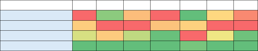
Figure – 9 Porolio’s yearly returns. (Dark Green Means Highest, Dark Red Means Lowest, Yellow means middle)
The equally weighted porolio consistently performed in between both the SPY and
Index weighted porolio from 2016 through 2022. The index weighted porolio outperformed
the SPY in every year but 2022, when the market turned south, and all 4 porolios felt large
losses. Not surprisingly, the index weighted porolio, as well as the equally weighted porolio,
appeared to follow a similar trend as the SPY in terms of yearly and monthly returns. The index
weighted porolio outperformed the index in 6 out of the 7 years, making a case for itself as the
smartest investment during this period. While the index weighted porolio did appear to
perform beer on a year-to-year comparison as well as overall, the drasc loss in 2022 cannot
be ignored. Since the largest stocks of the S&P500 have the largest eect on the returns of the
index, the other 490 stocks mainly aid the index by diversifying some of the largest stocks’
losses in bad years. As a result, while a porolio of the largest ten stocks in the S&P500 would
19
appear to produce superior returns in years when those companies did well, the lack of
diversicaon outside of those stocks, would lead to larger losses in years when these stocks did
not perform well. What can be seen by looking at the SPY, XLG, and index weighted porolios is
that as the porolio becomes less diversied in its holdings (500,50,10 stocks), the returns
appeared to become larger but change more drascally on a yearly basis.
It has long been taught that passively managed porolios outperform acvely managed
ones over the long-term. However, the superior returns of the test porolios do oer some
potenal that a combinaon of acvely managing the composion of the porolio while
passively invesng the money could outperform the market in the short-run and potenally
even in the long run. Whether or not these larger returns are accompanied by addional risk
will be invesgated next.
Standard Deviaon Comparison – Yearly and Monthly Basis
Now that I have invesgated the monthly, yearly and total returns for each of the
porolios, I shall look at the risk involved in each. To measure each porolios’ risk, the standard
deviaon of each porolio was rst calculated using the monthly returns. The standard
deviaon of a porolio includes both systemac (market) risk and unsystemac risk. The
standard deviaons of each porolio’s monthly returns as well as the standard deviaon of the
SPY and XLG, between 2016 and 2022, are shown in gure 10 below.
Monthly Return SD
(2016-2022)
Yearly Return SD
(2016-2022)
SPY
4.79%
14%
XLG
4.87%
21%
Equal Weighted
5.44%
25%
Index Weighted
5.71%
28%
20
Figure 10 – Comparison of Porolio Standard deviaon
We can see from the table above, as well as in Figure 11 below, that all the porolios
had similar risk structures. Each test porolio’s standard deviaons only varied above the
market’s by less than 1% each month. Yet when comparing the yearly return’s standard
deviaons, the increased variability that the test porolios experienced was made even more
evident. The porolios containing only the largest 10 stocks of the S&P500 would clearly have
more variability in their returns than that of more diverse porolios like the SPY or XLG.
Addionally, as I would expect, the equally weighted porolio, with its lower concentraon risk,
had a lower standard deviaon than the market-cap weighted porolio during every year.
STANDARD DEVIATION
2016
2017
2018
2019
2020
2021
2022
SPY
2.21%
1.85%
4.90%
3.25%
7.65%
3.81%
7.11%
XLG
2.66%
1.41%
4.61%
3.84%
7.51%
3.44%
6.90%
EQUAL WEIGHTED
2.92%
1.68%
5.21%
4.36%
7.24%
3.93%
8.38%
INDEX WEIGHTED
3.29%
1.88%
5.43%
4.37%
7.64%
4.45%
8.43%
Figure 11 – Porolio Monthly return standard deviaon for each year in study. (red means low, green means high, goes by year)
Beta
The beta of each stock is comprised of the market’s variance and the stock returns’
covariance. Variance measures how far apart the market’s data points spread out from their
average, while covariance measures how changes in a stock’s returns are related to changes in
the market’s returns. When the covariance of the stock is divided by the variance of the market,
the beta of the stock is produced. To calculate each porolio’s beta, I rst found the beta each
21
year, of the ten largest stocks. To determine the porolio beta for the year, these individual
stock betas were then weighed in accordance with their test porolio. The equally weighted
porolio would average the beta out evenly among the stocks, while the index weighted
porolio would allow for the largest stocks to inuence the beta more. Another way I found the
beta of the test porolios was to run the EXCEL slope funcon on the returns of the test
porolios and SPY, which unsurprisingly returned the same results as the previous method. The
beta of the test porolios was calculated using monthly and yearly returns and we will
invesgate the results in the secon below.
The monthly returns of the equally and index weighted porolios were found to have
had a 1.06 and 1.08 beta respecvely throughout the enre period. This means that the
monthly returns of both test porolios moved more dramacally in the face of market changes
than did the S&P500. While the monthly returns of the test porolios did experience a beta
above 1, there were mulple years where the betas were below 1. However, a beta of .90 is sll
considered very high and would indicate that the test porolios were only slightly less volale in
those years. Figure 12 through 14, below, depicts the betas for the test porolios on a yearly
basis as well as two dierent measures of the porolios’ beta during the enre period.
Beta of Monthly Returns
Equal W
Index W
XLG
2016
0.93
0.98
0.94
2017
0.92
0.99
1.00
2018
1.12
1.13
1.00
2019
1.10
1.09
1.00
2020
0.91
0.93
0.96
2021
1.09
1.09
0.99
2022
1.13
1.11
1.00
Figure 12 – Porolio Beta of each year – using Monthly returns for each year (2016-2022)

22
Equal W
Index W
XLG
Beta of Monthly Returns (84-Count)
1.06
1.08
.996
Figure 13 – Porolio Beta of enre period – Using Monthly Returns for enre period (2016-2022)
Equal W
Index W
XLG
Beta of Yearly Returns
1.34
1.46
1.13
Figure 14 – Porolio Beta of enre period – Using yearly Returns for enre period (2016-2022)
Since both the test porolios’ monthly returns experienced posive betas each year of
the study, the idea that the largest stocks could greatly outperform the market without adding
risk can be brought under serious queson. With the beta of the test porolios yearly returns
being found to be 1.34 and 1.46, this brings the idea even more under scruny. But all hope is
not lost. While these test porolios have indeed been proven to increase the volality of the
porolio, as their high betas represent, it is yet to be seen whether or not they sll produced
adequate returns for risk-averse investors to have chosen to accept their addional risk.
The benets of calculang the betas of these porolios using their monthly returns
included having a higher frequency of data points to give us a beer idea of short-term
uctuaons, as well as increased sensivity, as using monthly returns allows for a more granular
analysis of how a porolio reacts to market movements. The benets of using yearly returns, on
the other hand, is that yearly returns smooth out short-term uctuaons, giving us a beer
long-term perspecve. While each method has its benets and drawbacks, they both provide
valuable informaon about the volality of the porolios and give us some insight into how
returns will behave on a yearly and enre period basis.
Invesng Scenarios
23
To get a beer picture of how investors could ulize these test porolios, a couple
invesng scenarios were conducted. Each scenario assumed that an investor would invest
$1000 into one of the four porolios only diering in their investment frequency. To begin, my
rst scenario analysis assumed that an investor would invest $1000, starng on January 1
st
,
2016, into each of the porolios for each month and realize a return. The manager would then
reinvest $1000 into the porolio for the next month, keeping the weight the same as at the
beginning of the year, only changing stocks and weights at the beginning of the next year. These
monthly returns, added together throughout each year, provide us with the simplest form of
the investor’s total returns for the 7 years. In this scenario the index weighted, equally
weighted, XLG and SPY porolios would produce returns of 108.95%,95.62%, 85.97% and
83.76% respecvely. The benet of this invesng scenario is that it allows us to invesgate each
month’s returns separately, without the eect of compounding. What I discovered was that the
SPY experienced the most months with a posive return (58), the equally weighted porolio
was close behind with 57, and both the XLG and market-cap weighted porolios had posive
returns 55 mes. This means that the porolio with the lowest total return also had the most
posive monthly returns. This is because the SPY did have more months of growth, but the
other porolios, with their larger betas, produced larger returns during their good months that
ulmately made up for their addional few months of losses. Interesngly, while this scenario’s
yearly returns were obviously less than those that allowed for compounding in most years, this
scenario performed the best in 2018 for all four porolios. While every porolio felt a loss in
2018, this scenario’s porolios experienced the smallest loss, as losses too are not compounded
in this scenario. Ulmately, this scenario yet again depicts the larger variance of the test

24
porolios and demonstrates that this scenario’s returns would be much smaller than if an
investor were able to let their investment compound for the enre 7-year period.
The second invesng scenario assumed that the investor would invest $1000 into each
of the porolios at the beginning of each year and wait to fully realize and withdraw their gains
only aer that year ends. Aer rebalancing the porolios at the beginning of each year, the
investor would then only invest $1000 into each porolio at the start of the new year. This
scenario would garner some of the benets of compounding, and would produce returns of
126.27%, 108.28%, 92.94% and 83.41% for the index weighted, equally weighted, XLG and SPY,
respecvely. While this scenario would take some advantage of compounding returns, each year
the $1000 would only compound for 12 months. This scenario allows us to get a sense for how
these porolios dier depending on year and allows us to see trends in the long-term. While
this scenario takes advantage of compounding, there is sll one more scenario to maximize
investor returns.
In the third scenario, the investor would invest $1000 into each of the porolios on
January 1
st
, 2016, and leave the total value of the investment in the porolios for the enre 7-
years. This scenario diers from scenario two because while the investor would sll rebalance
his porolio yearly, choosing the new largest 10 stocks each year and weighing them
accordingly, they would reinvest their inial $1000 as well as any money they had made from
previous years. If investors let their money grow and were able to reap the full benets of
compounding returns, then the index weighted, equally weighted, XLG and SPY, would
experience returns of 158.09%,128.84%, 113.31% and 113.04%, respecvely. In this scenario,
25
both the equally weighted porolio (128.84%) and index weighted porolio (158.09%) would
vastly outperform the index in terms of total returns.
While analyzing the enre holding period return can be useful for comparing which
porolio would perform the best in the long run, it can vastly depend on starng and ending
points. As an example of this, if in this analysis I had placed the end date at the end of 2021, all
three porolios’ total returns would be higher, because up unl 2022, all four porolios had
experienced only posive, or near posive yearly returns. In 2022, however, both test porolios
compounded returns sharply fell by 142.57% and 115.62% respecvely. These large losses over
the nal year of the analysis vastly underperformed the index, which only felt a loss in its
compound returns of 47.61% in 2022. A summary of all the porolios compounded returns for
each year can be seen in gure 19, later in this paper.
While compounding returns are obviously benecial for every investor, what is yet to be
seen is whether these larger returns would sll be present if all three porolios were compared
on an equally risk-adjusted basis. To determine whether these porolios’ returns actually
provide superior results to that of the S&P500, a risk-adjusted analysis was completed to
determine how much return was added per percentage of risk for each porolio.
Analysis Limitaons
The limitaons to this research begin with only having access to returns from 2016 to
2022, and therefore this research may not reect the enre history of the S&P500 or accurately
predict its future. While this research can be useful for porolios that can be le and
rebalanced yearly, this may not work for some investors who are seeking to acvely trade their

26
stocks and rebalance their porolios daily, monthly, or quarterly. This research addionally has a
limitaon of only using the stocks and index weights of the ten largest market cap stocks in the
S&P500 index as of the beginning of each year. Therefore, while this analysis can give us a rough
esmate of how a porolio of the ten largest stocks would perform, it would not account for
changes in individual stock market capitalizaons and index weights throughout the year,
potenally vastly changing returns and variability.
Risk-Adjusted Comparison
To beer compare the returns of these porolios, a risk-adjusted analysis was completed
to decern which porolios performed the best when holding risk constant. A risk-adjusted
analysis is meant to discern how well porolios perform above the risk-free rate in relaon to
their volality. Therefore, to begin my analysis, the risk-free rate, as measured by 1-year T-bills,
for each month between January 2016 and December 2022 was collected. Then, the excess
returns of the equally weighted porolio, index weighted porolio, XLG, and SPY were
calculated, and their average monthly excess returns discovered. In this secon I computed the
Sharpe rao, Treynor rao, and Jenson’s Alpha to compare my three porolios on a risk-
adjusted basis. A summary of the results of this risk-adjusted analysis is shown below in gure
15.
Equally Weighted
Index Weighted
XLG
S&P500
Sharpe
12.61
13.24
13.25
13.73
Treynor
62.59%
67.98%
62.54%
63.48%
Alpha
0.0006
0.0020
0.0001
0
Figure 15 – Risk-Adjusted Rao Analysis Summary
Sharpe
27
To begin my risk-adjusted analysis, the Sharpe measure was rst calculated for each
porolio. To calculate the Sharpe rao, rst the risk-free rate was subtracted from each
porolio’s monthly returns. Then, each porolio’s total excess returns for the 7-year me period
were calculated, as well as the standard deviaon of the porolios’ raw returns. Once the
excess returns and standard deviaon for each porolio was calculated, each porolio’s excess
returns were divided by their standard deviaon. These raos resulted in Sharpe measures of
12.61, 13.24,13.25 and 13.73 for the equally weighted, index weighted, XLG and SPY,
respecvely.
The Sharpe rao is a mathemacal expression that considers the porolio’s excess
returns in relaon to its volality and risk over me. Essenally, the formula is used to quanfy
the total amount of excess returns earned above the risk-free rate, per unit of risk taken. The
Sharpe rao formula subtracts the risk-free rate on a 1-year T-bill, from the monthly historical
return of the porolio and divides the result by the porolio’s standard deviaon. The standard
deviaon of a porolio’s returns is a measure aimed at considering both the systemac and
unsystemac risk that the porolio contains. By dividing the excess returns of each porolio by
their standard deviaon, the Sharpe rao puts them all on the same risk-adjusted level, and by
doing so, aims to discover which porolio will produce superior returns when accounng for its
total risk. The porolio with the highest rao is the one that produced the largest excess returns
with the smallest level of total risk.
The excess returns of each of porolio can give us insight into their performance before I
even divide by their standard deviaon. The excess returns, standard deviaon, and beta, for
each porolio can be seen below in gure 16. What the ndings in gure 16 depict, is that while
28
the two test porolios clearly have larger excess returns, they also have larger standard
deviaons. The queson that the Sharpe rao answers then is, how much more risk is added to
those porolios to garner those larger returns? As well as is the risk added low enough to
warrant investment into those porolios rather than the S&P500?
A higher Sharpe measure is always desirable, as it means the porolio has garnered
larger returns relave to its risk and therefore it is a beer investment decision than lower
raoed porolios. Simply put, what a higher Sharpe rao directly means is that holding risk
constant for all porolios, the porolio with the highest rao will produce the largest returns. A
generally accepted benchmark for what is considered a “good Sharpe measure” would be
anything above 3, which all this study’s porolios fall far above.
What can be discovered by looking at the porolios’ Sharpe raos is that, while all the
porolios I evaluated performed well over the period, none outperformed the SPY on both a
systemac and unsystemac risk-adjusted comparison. What can be discerned from this
research is that, while the index weighted and equally weighted test porolios did perform
almost as well as the XLG, the much more diversied SPY remained the most resistant to
volality. The SPY, while producing smaller returns than the test porolios, would sll be the
best choice for a risk-adverse investor. While this rao can give us useful insights into which
porolio might be the best investment decision for investors, it does not give a complete picture
of the porolio return and risk relaonship.
Drawbacks of Sharpe’s Measure
29
There are a few drawbacks to the Sharpe Rao that can make it untrustworthy as a
standalone metric. To begin, the rao is calculated in an assumpon that investment returns are
normally distributed, which results in relevant interpretaons of the Sharpe rao potenally
being misleading. The rao’s eecveness can also vary based on the choice of the risk-free rate
and market benchmark. While for this analysis 1-year T-Bills and the SPY were selected as the
risk-free rate and market benchmark, other rates could have been selected. Another drawback
is that the risk-free and benchmark rates do not remain constant, meaning that while this
analysis’s ndings might be true for 2016-2022, the risk-free rate and benchmark are always
moving, causing this analysis to not necessarily reect future performance. The Sharpe rao
addionally, places relavely higher weight on short-term volality, which might not accurately
reect an investment’s long-term potenal. Despite these limitaons, the Sharpe rao remains
a valuable tool for assessing risk-adjusted returns.
Equally Weighted
Index Weighted
XLG
S&P500
Excess Return
68.65%
75.64%
64.51%
65.72%
Standard Deviation
5.44%
5.71%
4.87%
4.79%
Monthly Return Beta
1.06
1.08
.996
1
Figure 16– Sharpe and Treynor Measure Component Informaon
Treynor’s Measure
Treynor’s rao is another risk-adjusted measure that is similar to Sharpe’s rao in many
aspects. Both metrics aempt to measure the risk-return trade-o in porolio management by
dividing the excess returns of porolios by a measure of risk. While the Sharpe rao aims to
capture all elements of a porolio’s total risk (systemac and unsystemac) by dividing excess
returns by standard deviaon, the Treynor rao only captures the systemac component by
30
dividing the porolios excess returns by the porolio’s beta. By dividing the excess returns by
the beta, the Treynor rao only seeks to see how much systemic risk the porolio contains and
does not account for the unsystemac risk associated with the individual monthly returns. This
dierence in focus on systemac vs total risk is why most investors choose the Treynor rao
over the Sharpe rao for a well-diversied porolio. For this paper however, since the test
porolios are not well diversied, but the XLG and SPY are, I will ulize both measures to try to
get the most comprehensive insight possible.
Similarly to the Sharpe measure, the Treynor measure begins with compung the excess
return of the porolios relave to the risk-free rate. This me, instead of dividing by the
standard deviaon, I divided the excess returns by the porolio’s beta, which is a measure of
systemac risk. The Treynor measure, excess returns, and betas of the monthly returns for each
of the three porolios is shown below in gure 17. What we can see once the Treynor measures
are computed, is that while the SPY resulted in a posive 63.48% rao and outperformed both
the XLG and equally weighted porolios, the Index weighted test porolio outperformed the
market with a Treynor measure of 67.98%. This means that on a risk-adjusted basis, only
accounng for systemac risk, the index weighted porolio would outperform the market
during this period. This could be aributed to the index weighted porolio having the highest
beta and the market mainly experiencing only growth years during this study, with only the nal
year of the analysis seeing any real downturn. This could also be due to the rao only taking
into account systemac risk, as it does not include the unsystemac risk that the non-well-
diversied porolio could bring.
31
Equal W
Index W
XLG
SPY
Treynor
62.59%
67.98%
62.54%
63.48%
Excess Returns
68.651%
75.636%
64.505%
65.719%
Beta
1.06
1.08
0.996
1.00
Figure 17 – Treynor Measure Component Informaon
What these two measures tell us then, is that while the top 10-stock porolios do
outperform the S&P500 index in terms of total returns, and the index weighted porolio does
outperform the index on a systemac adjusted basis, all three test porolios underperform the
benchmark in terms of total risk-adjusted returns. Because all three of these porolios are not
as well diversied as the SPY, I would put more weight into the results of the Sharpe measure
and conclude that while the test porolios do garner larger returns, they do so at the sake of
adding unproporonately larger risk. As a result of the high unsystemac risk associated with
my two top-10 stock porolios, I can begin to condently say that while these two porolios
outperform the S&P500 in terms of total raw returns, they are not superior in terms of risk-
adjusted returns.
Jenson’s Alpha
The third risk-adjusted measure I will compute is Jenson’s alpha. Jenson’s alpha is a
measure that quanes the excess returns obtained by a porolio of investments above the
returns implied by the capital asset pricing model (CAPM). Alpha is dened as the incremental
returns from a porolio of investments, typically consisng of equies, above a certain
benchmark return (Jensen’s Measure, 2024). When using Jensen’s measure, the chosen
benchmark return is the Capital Asset Pricing Model, rather than the S&P500 market index.
Aer calculang the porolios return, risk-free rate, porolio beta, and expected market return,
32
I can calculate Jenson’s alpha. This analysis was done on Excel, so to begin, each porolio’s
excess returns were calculated, and a regression was done on the returns of each porolio.
Once the regression was completed, the intercept of the test porolio and SPY’s monthly
returns was found in the summary table and noted as the porolio’s alpha. The results of this
analysis can be seen in gure 15 back on page 27.
A good Jenson’s alpha measure is usually considered anything posive, as this posive
number indicates that the porolio outperformed the benchmark on a risk-adjusted basis over
the me period. When an investment has an alpha of one, it means that its return during the
specied me frame outperformed the overall market average by 1%. If the measure were to
come back as zero, the porolio would be said to be priced fairly, as it returned exactly what
was esmated by the CAPM. The S&P500, as represented by the SPY in this analysis, is an
example of a 0-alpha porolio, as it itself is the benchmark for which alphas are compared. If a
porolio’s result is negave, however, the porolio could be seen as underperforming its
expected return and could be viewed as a poor investment decision. In general, for return-
oriented investors, a posive, higher Alpha is always the desired outcome.
As we can see from the table above, all four of this study’s porolios had very low
alphas. This means that all four of the porolios were priced fairly for their experienced return
and risk throughout the period. This also means that all four of the porolios realized returns
would have compared favorably with the return associated with the level of expected risk. As
with many of this analysis’s other measures, the index weighted porolio had the largest alpha,
with equally weighted coming in second, and the XLG being barely above the market.
33
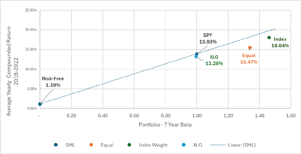
This relaonship can be easily seen on a graph, when the Security Market line is ploed,
and the porolio’s alpha’s shown in relaon. The graph will be set up with the X-Axis
represenng the beta of the porolio’s yearly returns and the Y-axis showing each porolio-
related yearly average return. To begin, a porolio only containing assets with the risk-free rate
is ploed. The average return of the risk-free rate during 2016-2022 was 1.19% and since an
asset with the risk-free rate has no systemac risk, its beta is 0. Aer the risk-free rate had been
marked, the S&P500, as measured by SPY, was ploed and the Security Market Line drawn
between them. What was found was, that during 2016 to 2022, the average return for the
S&P500 was 13.93%, which would mean a 12.74% market risk premium.
Figure 18– The SML on investments invested from 2016 through 2022.
The security Market Line above depicts dierent levels of systemac risk (or market risk)
for the dierent porolios. The line plots the porolios betas against the expected return of the
34
enre market at any given me. The SML can help analysts determine whether a porolio
would oer a favorable expected return compared to its level of risk. All stocks or porolios who
lie above the SML are considered undervalued because they oer larger returns compared to
their inherent risk. Porolios above the line are superior to those stocks or porolios with the
same or larger beta below the SML. Therefore, the two test porolios, while indeed producing
superior returns to that of the SPY and XLG, also lie below the SML. This means that the test
porolios would unproporonately add risk compared to their returns. Through my Jenson’s
alpha comparison then, the Equal weighed and Index weighted porolios would appear to
underperform the market in terms of proporonately adding risk for return. This does not make
the porolio useless, however, because for risk-neutral and risk-loving investors the added
returns that these test porolios produce could sll be worth the added risk that they would
have to accept.
Risk-Adjusted Comparison Summary
We can see through my risk-adjusted comparison of the four porolios that while the
two top-10 stock test porolios did underperform the market benchmark on a total risk-
adjusted basis (Sharpe measure), they did outperform the market when adjusted for only their
systemac risk (Treynor Measure). This is not surprising as the SPY is very well-diversied, with
over 500 or so stocks, but my two test porolios have much less ground to spread their
variability over. My risk-adjusted analysis indicates then that the test porolios did perform well
in terms of the systemac risk they contained, however, they also had high unsystemac risk
due to the fact that they only contained ten stocks. The small size of the test porolio means
even if only a few stocks have a bad month, then the whole porolio could be greatly aected.
35
Ulmately then, for investors interested in the high returns these test porolios can oer, they
must also be willing to accept the added unsystemac risk that comes with the simplicity of
these porolios.
Alternave Analysis: What if the analysis ended aer 2021?
If the analysis were to have ended at the end of 2021 the compounded returns of all
four of these porolios would have been much higher. When compung the compounded
returns of the porolios it is clear to see when would have been the ideal me to have
withdrawn our funds. Figure 19 below shows the compounded returns at the end of each year
of this study. Clearly, the end of 2021 would have been the ideal me to have withdrawn funds
invested in any of these porolios, but would the test porolios have performed any beer on a
risk-adjusted basis? To discover the answer to that queson, I performed the same analysis as
above, but only included data through the end of 2021.
Yearly Returns Compounded
2016
2017
2018
2019
2020
2021
2022
1 Year
Return
2 year
return
3 Year
Return
4 Year
Return
5 Year
Return
6 Year
Return
7 Year
Return
SPY
12.00%
36.42%
30.09%
70.87%
102.33%
160.65%
113.04%
Equal
16.17%
52.86%
50.04%
106.04%
169.53%
244.46%
128.84%
Index
14.92%
53.16%
53.41%
115.47%
203.78%
301.66%
158.09%
XLG
11%
37%
32%
74%
116%
182%
113%
Figure 19 – Porolios’ Yearly Compounded Returns from one to seven years (2016-2022)
As we can see, throughout the rst six years, the index and equally weighted porolios
vastly outperformed the market in terms of total compounded returns, with the XLG slowly
surpassing the market throughout the period. During the rst six years of this study the test
porolios also outperformed the market when adjusted for both total and only systemac risk,
most likely due to the sheer size of their returns. The Sharpe and Treynor measures, as well as

36
Jenson’s alpha for each of the porolios monthly returns from 2016-2021 are show below in
gure 20. Aer replong the porolios on a new graph, it was discovered that both test
porolios as well as the XLG, all appeared above the SML for the rst six years and
outperformed the market in terms of risk and return. This means that, at least for the rst six
years of this study, investors of all risk preferences would ideally have chosen my test porolios
or the XLG over invesng in the market.
Equally weighted
Index Weighted
XLG
S&P500
Sharpe
32.72
35.46
28.76
27.01
Treynor
148.43%
168.08%
126.12%
115.79%
Alpha
0.0041
0.0061
0.0014
0
Figure 20 – Alternave Analysis – Risk-Adjusted Analysis Summary
Figure 21 – The SML on investments invested from 2016 through 2021.
Research Findings Summary
This research’s test porolios were designed specically to invesgate how much weight
the ten largest stocks in the S&P500 carried, and whether a porolio of just those stocks could
SPY
17.96%
Risk-Free
1.23%
Equal
23.64%
Index
27.00%
XLG
19.55%
0.00%
5.00%
10.00%
15.00%
20.00%
25.00%
30.00%
- 0.20 0.40 0.60 0.80 1.00 1.20 1.40 1.60
Average Yearly Compounded Return
2016-2022
Portfolio - 7 Year Beta
SML Equal Index Weight XLG Linear (SML)
37
outperform the market in terms of total, yearly, and monthly returns on a risk-adjusted basis.
What this analysis discovered was that monthly, the test porolios outperformed the market far
more oen than they underperformed it. On a yearly basis, the test porolios outperformed
the market every year but 2022, where every porolio felt a massive drop o in returns, but the
test porolios specically felt a far worse impact than the market. While the test porolios did
outperform the market in the rst 6 years in terms of both raw returns and risk-adjusted
returns, their higher betas eventually led them to feel much worse reducons in their
compounded returns by the end of 2022. Overall, this loss in the nal year of the study did not
keep the test porolios from having larger total returns over the enre 7-years, as both the
index and equally weighted porolios sll were able to beat the market in terms of total
compounded returns from 2016 through 2022.
While the ten largest stocks in the index did perform well, and even performed very
closely to the market during these years, as the equally and index weighted 7-year monthly
return betas were only 1.06 and 1.08 respecvely, they did appear to have underperformed the
market in terms of total return per unit of total risk taken. While the porolios appeared to
outperform the market in terms of returns per unit of unsystemac risk taken, they failed to
surpass the market when the porolios’ total risk was accounted for. Because I sought to have a
hybrid invesng strategy, it was unsurprising to see my test porolios had near zero alphas.
While these alphas were slightly posive, indicang that they did produce returns larger than
expected for their level of risk taken, they were sll very low and should not be overvalued.
Therefore, while this study may not show that the largest stocks would outperform the total
index on a risk-adjusted basis, it does show that, the largest stocks in the S&P500 are
38
responsible for the majority of the index’s returns as well as its volality, while the rest of the
index would appear to be responsible for diversifying the returns and aiding in loss reducon in
bad years. My research showed that as the porolios grew and contained more stocks, their
returns would diminish, but so would their variability. What can be seen then from this analysis,
is that while the equally weighted and index weighted test porolios may not contain enough
stocks to adequately diversify their returns, the XLG, with its 50 component stocks, did appear
to barely outperform the index in terms of both its compounded raw returns and risk-adjusted
metrics. The XLG experienced superior raw returns for most of the years analyzed and even had
the lowest porolio standard deviaon of monthly returns for 4 of the 7 years. The XLG also
experienced yearly betas of exactly 1 or less, meaning it reacted to market changes the same or
even slightly less than the SPY. Therefore, on a risk-adjusted basis, the XLG outperformed the
SPY when it comes to all measures analyzed for the 7 years. On the Security Market Line,
however, the XLG appeared to barely underperform the market, as its 7-year beta was near 1,
yet it garnered a slightly lower average yearly return than the SPY. Altogether, my research
would appear to demonstrate that the index can be beaten in the short-term and even can
potenally be beaten in the long-term, albeit only slightly, and that more than the 10 largest
stocks are required in order to maintain proper diversicaon. While my test porolios may not
have outperformed the market on a risk-adjusted basis for the enre 7-year period, I was able
to see that in cases of bull markets, that this investment strategy could be a wise investment
decision.
Overall, even though I have proven that my test porolios cannot outperform the
market in the long term, they are not useless. Both test porolios sll performed well during
39
most of the years analyzed and while they did not perform well enough during the enre period
to beat the market on a risk-adjusted basis, they did ulmately produce larger compounded
returns. The fundamental principle of the risk-return tradeo holds true for the test porolios,
as in search of the larger returns both could in fact have generated, an investor would have also
had to accept their larger risk/volality. This would mean that for investors who are risk-neutral
or risk-loving, these porolios would have been aracve during these years. However, even
risk-adverse investors could have been interested in these porolios, had they only been
working with informaon from the rst six years. While there are ways to match the market and
even surpass it slightly with less than 500 stocks, in the long run, the sheer size and diversity of
the S&P500 index protects it from many of the unsystemac risks that can arise in a smaller, not
as well-diversied porolio. While managers can outperform the market on year and even
mul-year stretches, this research shows that the passively managed S&P500 index, with its use
of proporonately market cap weighted stocks, allows for it to be beer prepared for both bull
and bear markets and perform the best in the long run.
40
Works Cited
D'Antuono, M. (2023, February 13). Monthly_Stock_Return_Data. Murray, Kentucky, United
States of America.
FINHACKER. (2024, February 11). Top 20 S&P 500 Companies by Market Cap (1990 – 2024).
Retrieved from FINHACKER.cz: hps://www.nhacker.cz/top-20-sp-500-companies-by-
market-cap/#2024
Friedberg, B. (2018, November 28). Know Which Weighted-Index Fund to Choose. Retrieved
from USNews: hps://money.usnews.com/invesng/funds/arcles/which-are-beer-
equal-weighted-or-cap-weighted-index-funds
Jensen’s Measure. (2024, February 20). Retrieved from WallStreet Prep:
hps://www.wallstreetprep.com/knowledge/jensens-measure-alpha/
KENTON, W. (2023, Septemer 22). S&P 500 Index: What It’s for and Why It’s Important in
Invesng. Retrieved from Investopedia:
hps://www.investopedia.com/terms/s/sp500.asp
Multpl. (2024, March 26). 1 Year Treasury Rate by Year. Retrieved from Multpl:
hps://www.multpl.com/1-year-treasury-rate/table/by-year
Reeves, J. (2024, February 2). 5 Best S&P 500 Index Funds Of February 2024. Retrieved from
Forbes: hps://www.forbes.com/advisor/invesng/best-sp-500-index-funds/
Sather, A. (2023, July 12). Historical S&P 500 Industry Weights – [20+ Year History]. Retrieved
from EInvesng For Beginners: hps://einvesngforbeginners.com/historical-sp-500-
industry-weights-20-years/
SlickCharts. (2024, April 5). S&P 500 Total Returns. Retrieved from SlickCharts:
hps://www.slickcharts.com/sp500/returns
SPY VS. SPYD. (2024, March 26). Retrieved from Porolio Labs:
hps://porolioslab.com/tools/stock-comparison/SPY/SPYD
41
Webster, I. (2024, February 27). S&P500 Data. Retrieved from S&P500 Data:
hps://www.ocialdata.org/us/stocks/s-p-500/2000?amount=1000&endYear=2023
Yahoo Finance. (2024, April 5). Invesco S&P 500 Top 50 ETF (XLG). Retrieved from Yahoo Finance:
hps://nance.yahoo.com/quote/XLG/history?period1=1451606400&period2=1669852
800&frequency=1mo
Yahoo Finance. (2024, April 5). SPDR S&P 500 ETF Trust (SPY). Retrieved from Yahoo FInance:
hps://nance.yahoo.com/quote/SPY/history?period1=1451606400&period2=1669852
800&frequency=1mo
