Towards a Homomorphic Machine Learning Big Data Pipeline for

the Financial Services Sector

Oliver Masters

, Hamish Hunt

, Enrico Steﬃnlongo

, Jack Crawford

, Flavio Bergamaschi

Maria Eugenia Dela Rosa

, Caio Cesar Quini

, Camila T. Alves

, Fernanda de Souza

, and Deise

Goncalves Ferreira

IBM Research, Hursley, UK

{oliver.masters,enrico.steffinlongo,jack.crawford}@ibm.com

{hamishhun,flavio}@uk.ibm.com

Banco Bradesco SA, Osasco, SP, Brasil

{maria.e.delarosa,caio.quini,camila.t.alves,fernanda.souza,deise.g.ferreira}@bradesco.com.br

Abstract. Machine learning (ML) is today commonly employed in the Financial Services Sector (FSS)

to create various models to predict a variety of conditions ranging from ﬁnancial transactions fraud to

outcomes of investments and also targeted marketing campaigns. The common ML technique used for

the modeling is supervised learning using regression algorithms and usually involves large amounts of

data that needs to be shared and prepared before the actual learning phase. Compliance with privacy

laws and conﬁdentiality regulations requires that most, if not all, of the data must be kept in a secure

environment, usually in-house, and not outsourced to cloud or multi-tenant shared environments.

This paper presents the results of a research collaboration between IBM Research and Banco Bradesco

SA to investigate approaches to homomorphically secure a typical ML pipeline commonly employed in

the FSS industry.

We investigated and de-constructed a typical ML pipeline used by Banco Bradesco and applied Homo-

morphic Encryption (HE) to two of the important ML tasks, namely the variable selection phase of the

model generation task and the prediction task. Variable selection, which usually precedes the training

phase, is very important when working with data sets for which no prior knowledge of the covariate set

exists. Our work provides a way to deﬁne an initial covariate set for the training phase while preserving

the privacy and conﬁdentiality of the input data sets.

Quality metrics, using real ﬁnancial data, comprising quantitative, qualitative and categorical features,

demonstrated that our HE based pipeline can yield results comparable to state of the art variable

selection techniques and the performance results demonstrated that HE technology has reached the

inﬂection point where it can be useful in batch processing in a ﬁnancial business setting.

Keywords: homomorphic encryption; variable reduction; variable selection; feature selection; pre-

diction

Table of Contents

Towards a Homomorphic Machine Learning Big Data Pipeline for the Financial Services

Sector . . . . . . . . . . . . . . . . . . . . . . . . . . . . . . . . . . . . . . . . . . . . . . . . . . . . . . . . . . . . . . . . . . . . . . . . . . . 1

Oliver Masters, Hamish Hunt, Enrico Steﬃnlongo, Jack Crawford, Flavio Bergamaschi,

Maria Eugenia Dela Rosa, Caio Cesar Quini, Camila T. Alves, Fernanda de Souza,

and Deise Goncalves Ferreira

1 Introduction . . . . . . . . . . . . . . . . . . . . . . . . . . . . . . . . . . . . . . . . . . . . . . . . . . . . . . . . . . . . . . . . . . . 3

2 Background . . . . . . . . . . . . . . . . . . . . . . . . . . . . . . . . . . . . . . . . . . . . . . . . . . . . . . . . . . . . . . . . . . . 4

2.1 CKKS in HElib . . . . . . . . . . . . . . . . . . . . . . . . . . . . . . . . . . . . . . . . . . . . . . . . . . . . . . . . . . . . 4

2.2 Homomorphic predictions . . . . . . . . . . . . . . . . . . . . . . . . . . . . . . . . . . . . . . . . . . . . . . . . . . . 4

2.3 Variable Selection via Logistic Regression . . . . . . . . . . . . . . . . . . . . . . . . . . . . . . . . . . . . . 5

3 Implementation . . . . . . . . . . . . . . . . . . . . . . . . . . . . . . . . . . . . . . . . . . . . . . . . . . . . . . . . . . . . . . . . 7

3.1 Pipeline Overview . . . . . . . . . . . . . . . . . . . . . . . . . . . . . . . . . . . . . . . . . . . . . . . . . . . . . . . . . . 7

3.2 Function Approximations . . . . . . . . . . . . . . . . . . . . . . . . . . . . . . . . . . . . . . . . . . . . . . . . . . . 8

3.3 HE logistic regression predictions . . . . . . . . . . . . . . . . . . . . . . . . . . . . . . . . . . . . . . . . . . . . 9

3.4 Homomorphic variable selection . . . . . . . . . . . . . . . . . . . . . . . . . . . . . . . . . . . . . . . . . . . . . . 10

4 Experimental Evaluation . . . . . . . . . . . . . . . . . . . . . . . . . . . . . . . . . . . . . . . . . . . . . . . . . . . . . . . . 11

4.1 Testing Environment . . . . . . . . . . . . . . . . . . . . . . . . . . . . . . . . . . . . . . . . . . . . . . . . . . . . . . . 12

4.2 CKKS Parameters . . . . . . . . . . . . . . . . . . . . . . . . . . . . . . . . . . . . . . . . . . . . . . . . . . . . . . . . . 12

4.3 Dataset preparation . . . . . . . . . . . . . . . . . . . . . . . . . . . . . . . . . . . . . . . . . . . . . . . . . . . . . . . . 13

4.4 Results and discussion . . . . . . . . . . . . . . . . . . . . . . . . . . . . . . . . . . . . . . . . . . . . . . . . . . . . . . 13

5 Conclusion . . . . . . . . . . . . . . . . . . . . . . . . . . . . . . . . . . . . . . . . . . . . . . . . . . . . . . . . . . . . . . . . . . . . 16

6 Further Work . . . . . . . . . . . . . . . . . . . . . . . . . . . . . . . . . . . . . . . . . . . . . . . . . . . . . . . . . . . . . . . . . . 17

Acknowledgements . . . . . . . . . . . . . . . . . . . . . . . . . . . . . . . . . . . . . . . . . . . . . . . . . . . . . . . . . . . . . . . . 19

References . . . . . . . . . . . . . . . . . . . . . . . . . . . . . . . . . . . . . . . . . . . . . . . . . . . . . . . . . . . . . . . . . . . . . . . 19

A Model Evaluation Metrics . . . . . . . . . . . . . . . . . . . . . . . . . . . . . . . . . . . . . . . . . . . . . . . . . . . . . . . 21

1 Introduction

Homomorphic encryption (HE) promises to generally transform and disrupt how business is cur-

rently done in many industries such as, but not limited to, healthcare, medical sciences, and ﬁnance.

One particular area of interest and value to apply HE across numerous industries is in machine

learning (ML). The ability to compute directly on the encrypted data allows that data to be shared

in areas that were once considered impossible or highly undesirable due to data leaks through single

point of failure (individuals or systems with the authority to see the data) which could be insecure.

Today, organizations make far more use of vast amounts of aggregated data to be able to perform

data analytics and ML. Many organizations ﬁnd themselves restricted from sharing data, internally

and externally, due to legislation, regulation, and their other need-to-know policies coming into

direct conﬂict with the need to collaborate by sharing the data (a.k.a. need-to-share). Approaches

leveraging homomorphic encryption can overcome these restrictions by allowing homomorphic data

aggregation intra- and/or inter-organization; meaning that a computation requiring the aggregated

data can be performed without other parties having access to data shared in the aggregation.

HE as a technology has undergone accelerated progress since Gentry’s inﬂuential work [13]

showed how to construct a fully homomorphic encryption scheme based on lattices. Several schemes

and algorithmic improvements have emerged since Gentry such as the BGV [5] and FV [12] schemes.

The community is aware that the technology is becoming adequately performant to be useful and/or

disrupt several areas [1]. In the last few years, the CKKS scheme [9] has emerged oﬀering a more

natural setting for performing operations on approximate numbers. CKKS is thus generally more

suitable to analytics and ML problems.

The terminology Machine Learning, ﬁrst introduced by Arthur Samuel in 1959 [25], today com-

prises several tasks with the fundamental goal of creating a model that can make predictions. Model

generation by learning is the main focus of ML and the motivation in doing this homomorphically

has been around for a few years. Many solutions have been shown to perform this task with varying

times from minutes to hours using diﬀerent HE schemes [20,8,4,21,10,16]. However, practitioners

are aware that in a typical ML pipeline this is but one necessary task.

Our work consists of exploring two tasks in the ML pipeline that HE can aid in the sharing of

data. The ﬁrst is running the prediction of a generated logistic regression model. This is the task

that is the re-usable part of the typical ML endeavor. Businesses will want to ensure that only

certain parts of the business will have access to the model and/or data. Although this tends to be

inherently performed in the learning aspect it has had little attention to as a separate facet and

metrics on it seem somewhat limited in the literature. Moreover, in previous works [14,6] the speed

of prediction was achieved through having the model itself unencrypted, thus only providing privacy

of the input data. This work explores the concept of keeping the generated model private in addition

to the data. The second task that we explore is performing variable reduction or more precisely

variable selection (a.k.a. feature selection in the literature). With real data, this is a very common

machine learning pipeline phase in the model generation and necessary to avoid overﬁtting of the

data and/or only perform learning with variables of importance thus reducing resource required.

To achieve our goals, we apply state-of-the-art techniques in homomorphic encryption and

ML. For our homomorphic encryption and computations, we use the homomorphic encryption

library HElib [15], explicitly making use of its CKKS capabilities in the work presented. Firstly, we

take an existing, encrypted logistic regression model that constitutes sensitive intellectual property

and demonstrate the feasibility of running a large number of encrypted prediction operations on

real, encrypted ﬁnancial data while retaining acceptable performance with both 128 and 256 bits

of security. Secondly, we build on work by Bergamaschi et al. [2] by exploring the feasibility of

homomorphic variable selection.

2 Background

In this section, we will introduce the key concepts which will be required throughout this work. All

homomorphic computations were done using HElib’s CKKS capabilities that were introduced to the

library in 2018 [2,15]. This allows us to code using approximates of real numbers. To solve both ML

tasks of predicting and variable selection, this is required. The way we determine the importance

of a variable for variable selection is to use the evaluation of a logistic regression model trained on

that variable individually.

2.1 CKKS in HElib

The CKKS scheme [9] has provided a large change for certain problems of how we think about

applying HE. In HElib’s variant of the scheme the ciphertext mechanisms are mostly the same as

they are for the BGV scheme [2]. The main diﬀerence lies in the CKKS plaintext space which we

will take advantage of.

CKKS has a decryption invariant form of [hsk, cti]

pt, where sk and ct are the secret key and

ciphertext vectors, respectively, [·]

denotes reduction modulo q into the interval (−q/2, q/2], and

pt is an element that encodes the plaintext and includes also some noise. CKKS uses an element

of low norm, |

pt|  q. Decoding to a plaintext, pt, is given by

pt = e + ∆ · pt where ∆ is a scaling

factor and, ideally, after performing our necessary computation we still have |e| < ∆.

Due to working with approximations of real numbers the scheme supports varying levels of

precision determined by the accuracy parameter r. The noise, e, introduced during the encoding

of the plaintext causes each operation performed in the CKKS scheme to be accurate up to an

absolute bound on the magnitude of the additive noise, namely 2

−r

The HElib implementation of the CKKS scheme maps to a plaintext space that is the integer

polynomial ring Z[X]/hΦ

(X)i where Φ

(X) is the m

cyclotomic polynomial with degree given

by Euler’s totient φ(m). The scheme provides encode and decode procedures to map the native

plaintext elements to and from plaintext complex vectors v = C

where l = φ(m)/2 determines the

number of complex numbers that can be packed into a single plaintext. For our purposes, we only

make use of the real part of the numbers.

2.2 Homomorphic predictions

Given a trained ML model, its primary purpose is the generation of an output estimate of whether a

given input has the condition or not. This is known as prediction. Many types of predictive models

can be considered to be another form of data which can be encrypted homomorphically.

Depending on the scenario there are choices to be made as whether the data, the model or both

are homomorphically encrypted. In all cases, the output will be encrypted as an operation between

a ciphertext or a plaintext with a ciphertext always results in a ciphertext.

The ﬁrst proposal of a privacy preserving Encrypted Prediction as a Service (EPaaS) solution

was CryptoNets [14] in 2016. CryptoNets achieved 99% accuracy and a throughput of roughly 59000

predictions per hour.

When applying a prediction model in an HE context, careful consideration must be taken to

ﬁnd a balance between the accuracy and the computational complexity. This is due to the natural

overhead that is introduced by encryption. Previous work has been carried out to reduce both the

limitation on the depth and breadth of the circuit as well as the latency of such applications.

One such notable work to produce a low latency, homomorphic neural network known as LoLa [6]

presents an application that achieves considerable speedups without sacriﬁcing on the level of secu-

rity provided in previous attempts. This was achieved via the use of alternative data representations

during the computation process. This application exhibited the feasibility of performing homomor-

phic predictions however left the exploration of homomorphically performing the training of ML

models to further study.

It should be noted that these previous schemes do not perform the prediction using a homo-

morphically encrypted model thus making the prediction less computationally expensive.

2.3 Variable Selection via Logistic Regression

Variable selection is the process of deciding which of the variables (or features) of a given dataset are

important to be kept when generating a predictive model. This also determines the variables which

are not worth preserving as they have negligible or detrimental impact on the model’s predictive

quality [17,19].

Homomorphic model generation by learning is a topic of increasing interest due to the ability

to generate models with training data that is encrypted. This is important in scenarios where the

data used for the training is private. In particular medical data is considered highly conﬁdential

and there is focus on applying HE to this sector. Another key industry in which data privacy and

ML techniques are of particular interest is the ﬁnancial sector.

Most notably, the work [4,8,10,21] related to the 2017 iDASH competition [18] as well as [20,16,3]

explore the use of logistic regression on homomorphically encrypted data to generate models. These

achieve varying computation times for data samples of diﬀering sizes. Applications range from 6

minutes for over 1500 samples containing 18 features in [20] to generating a model from over 420000

samples containing over 200 features in approximately 17 hours [16]. These works demonstrate

both the reality of generating a model homomorphically in a feasible amount of time as well as the

scalability of such methods to handle large datasets.

Our work focuses on the variable selection phase which precedes the training phase in a typical

ML pipeline. In addition, unlike previous work, our approach assumes and uses an empty covari-

ate set. This is very important when performing data analytics on data sets for which no prior

knowledge of the covariate set exists. Our solution provides a way to homomorphically determine

an appropriate initial covariate set for the training phase.

When attempting to predict a binary condition or attribute (also known as classiﬁcation) based

on other attributes given (not necessarily binary themselves), logistic regression is a standard ML

technique employed.

In this work, we are only dealing with the case where the condition that we want to predict

is binary (i.e. with condition or without condition). The data, which one can consider to form a

matrix, consists of n records or rows of the form (y

, x

) with y

∈ {0, 1} and x

∈ R

. The aim

is to predict the value of y ∈ {0, 1} given the attributes x, and the logistic regression technique

postulates that the distribution of y given x is given by

Pr[y = 1|x] =

1 + exp



−w

−

i=1



1 + exp (−x

where w ∈ R

d+1

is a ﬁxed vector of weights and x

= (1|x

) ∈ R

d+1

is a feature vector. Given the

training data {(y

, x

)}

i=1

, we can therefore make predictions if we can ﬁnd the vector w that best

matches this data, where the notion of best match is typically maximum likelihood. Such a weight

vector, w

∗

, can be expressed explicitly as

∗

= arg max







1 + exp



−x



1 + exp











where we use the probability postulate given above in conjunction with the following identity

1 −

1 + exp(−z)

1 + exp(z)

The formula for w

∗

can be written more compactly by setting y

= 2y

− 1 ∈ {±1} and

= y

· x

, then our goal is to compute or approximate

∗

= arg max

(

i=1

1 + exp (−z

)

= arg min

(

i=1

log



1 + exp



−z



)

For a candidate weight vector w, we denote the (normalized) loss function for the given training

set by

J(w)

def

i=1

log



1 + exp



−z



and our goal is to ﬁnd w that minimizes that loss.

Nesterov’s Accelerated Gradient Descent. We use Nesterov’s accelerated gradient decent [23]

which has been used successfully and applied previously in [2]. It is a variant of the iterative method

used by Kim et al. in [20]. Let σ be the sigmoid function,

σ(x)

def

= 1/(1 + e

−x

then the gradient of the loss function with respect to w can be expressed as

∇J(w) = −

i=1

1 + exp (z

· z

= −

i=1



−z



· z

Untrusted Container

Trusted Container

Simple

Key Management

Trusted Container

Financial

Data

Computation

Result

Data

Preparation

Data

Unencrypted

Clear

Computation

Encode

Encrypt

Data

Encrypted

Computati

Computation

Result

Encrypted

Decrypt

Decode

Computation

Result

Analysis

FHE Context

FHE Keys

Generator

Public key

+ Context

Secret key

+ Context

Secure Channel

Graphs

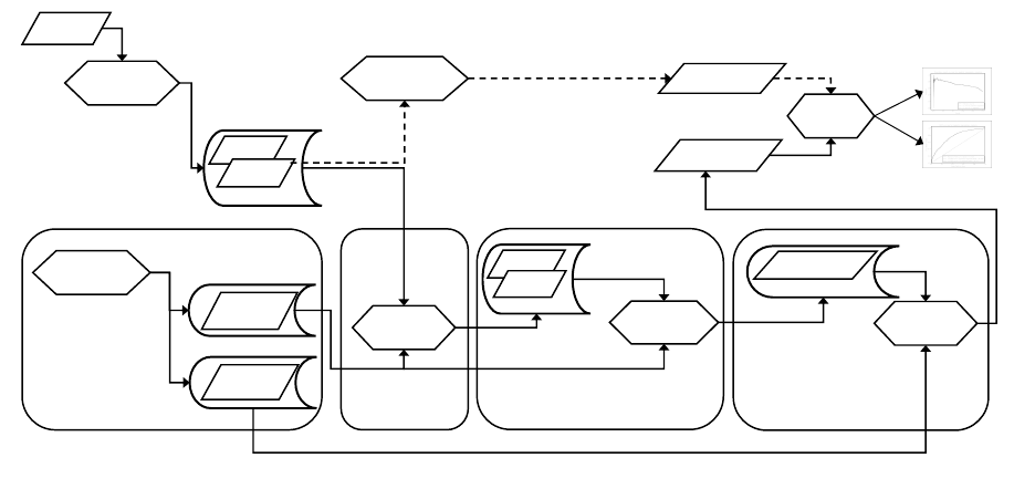
Fig. 1. Homomorphic and plaintext pipelines.

Nesterov’s method initializes two evolving vectors to the mean average of the input records.

Then each iteration computes

(t+1)

= v

(t)

− α

· ∇J



(t)



(t+1)

= (1 − γ

) · w

(t+1)

+ γ

· w

(t)

where α

, γ

are scalar parameters that change from one iteration to the next. The α parameter is

known as the learning rate and γ is called the moving average smoothing parameter. For how they

are set, see section 3.4.

3 Implementation

In this section, we will discuss our methodology for performing homomorphic predictions and ho-

momorphic variable selection. In the case of the logistic predictions, we provide a description of the

method used to eﬃciently pack data into CKKS ciphertexts as well as requisite function approxi-

mations employed. In the case of the variable selection, we provide greater detail of the technique

adopted for obtaining relevant scores for each variable as well as parameters and conﬁguration of the

Nesterov gradient descent algorithm. We present the modular ML pipeline of our experimentation.

3.1 Pipeline Overview

Figure 1 illustrates the basic model of the computation and ﬂow of data of the implemented

system, used for both prediction and variable selection. In this model, we have several parties

with the trusted parties operating in trusted containers (labeled 1, 2, and 4) and the untrusted

party operating in the untrusted container 3. Typically, this trust model would correspond to a

client-server relationship in which the server is considered to be acting under the honest-but-curious

attacker model.

The trusted container 1, hosted in a hardware security module, is responsible for key manage-

ment and generation of the public-private key pairs, and the key switching matrices required for

the computation, as described in [15]. For the sake of conciseness, we will henceforth refer to the

public key, the context, and the key switching matrices collectively as simply the public key.

Trusted container 2 is responsible for encrypting the plain data with the public key. The en-

crypted data is made available to container 3, the honest-but-curious untrusted environment where

the homomorphic computation can be performed. Both containers require and have access to the

public-key.

Trusted container 4 is responsible for decrypting the ﬁnal results using the secret key which is

accessed through a secure channel.

Considering the ﬂow of data through the system, ﬁrstly raw ﬁnancial data is sanitized and

pre-processed by the Data Preparation module, which then ﬂows into trusted container 2. The data

is then encoded according to the relevant Data packing method as described later on, which diﬀers

depending on whether prediction or variable selection is being performed. The encoded data is then

encrypted using the public key and then sent to the untrusted container.

The untrusted container 3 performs whichever homomorphic computation is required by using

the public key and encrypted data. In the prediction case, this will be an operation between en-

crypted data and an existing encrypted model as described in 3.3. In the variable reduction case,

this will be a large number of logistic regression model trainings followed by a log loss computation

as described in 3.4. In both cases, the encrypted output is passed to the trusted container 4 for

decryption. Trusted container 4 will decrypt the result with the secret key and then process it

directly or pass it elsewhere for usage.

In addition to this workﬂow, ﬁgure 1 also contains more steps which would not be used in a

typical system, but that we employed for evaluation purposes. These can be seen in the cells which

are connected with dotted lines. The Clear Computation block performs analogous computations

to the Encrypted Computation block, except they are performed with standard methods entirely

on the plaintext data. The results of the Clear Computation block and the HE pipeline are then

compared using standard statistical techniques. It is from this ﬁnal analysis step that the ﬁgures

seen in section 4.4 are derived.

3.2 Function Approximations

Our homomorphic computations necessitate the evaluation of several higher-order functions such

as sigmoid and logarithm. Despite the fact that addition and multiplication are the only operations

native to the CKKS scheme employed, we are able to use polynomial approximations of arbitrary

continuous functions. It was important to strike a balance between degree of polynomial approxi-

mation with higher degrees increasing the depth of the calculation and accuracy of approximation

which is harmed by lower-degree approximations. Due to the signiﬁcant disadvantages inherent to

high-degree polynomials, in terms of both computation time and noise growth, we use the lowest-

degree approximations possible which still yield good results.

Sigmoid approximation. For sigmoid function approximation, we use the same low-degree poly-

nomial function in a bounded symmetrical range around zero as in [20,2], namely with degree-3

and degree-7 approximation polynomials in the interval [−8, 8]

SIG3(x)

def

= 0.5 − 1.2





+ 0.81562





and (1)

SIG7(x)

def

= 0.5 − 1.734





+ 4.19407





(2)

−5.43402





+ 2.50739





Logarithm approximation. We apply the same technique to derive a quartic polynomial ap-

proximation function for the composition log ◦ σ directly rather than composing approximations

for both logarithm and sigmoid, since this allows us to perform the required computation with

minimal computational depth. We again use an approximation minimizing mean squared diﬀerence

in [−8, 8]:

LOGSIG4(x)

def

= 0.000527x

− 0.0822x

+ 0.5x − 0.78 (3)

3.3 HE logistic regression predictions

In this section, we describe a general implementation to perform logistic regression predictions.

This is achieved by encoding and encrypting both model and data. More precisely, taking data

that was segregated for testing from a real ﬁnancial dataset, the data was encoded and encrypted

then passed to the predictor. The predictor loads the required model and performs the prediction

algorithm. Essentially a inner product that is the input to a sigmoid function.

Data packing. To perform homomorphic logistic regression predictions, we require an encrypted

model and encrypted data. The model consists of a vector of weights β ∈ R

, where the 0

entry of

β is the bias term. In order to ﬁt best with our homomorphic implementation, we simply replicate

each entry β

, 0 ≤ i ≤ 16, into its own ciphertext. That is to say, we let m

be an encryption of

the vector u

∈ C

where each entry of u

is equal to β

. For packing of the data, we describe ﬁrst

the case where we have l predictions to perform, i.e. a set D of data where |D| = l. We pack all l

vectors {x

}

i=1

∈ R

into 16 ciphertexts by mapping the ﬁrst entry of each x into one ciphertext,

the second entry of every x into another ciphertext, and so on.

Prediction. If we denote the resulting ciphertexts {c

}

i=1

, we can perform l predictions by com-

puting

i=1

 m

where  is the entrywise product and σ is the sigmoid function (also computed entrywise in this

case). This amounts to an inner product operation on a vector of ciphertexts.

The resulting predictions will be one ciphertext which decrypts to a vector in C

corresponding

to l predictions. In order to perform n > l predictions, we simply partition the n data vectors into

e blocks, perform the prediction on each block, then concatenate the d

e vectors of size l at the

end. This can be performed completely in parallel for a large n.

The inner product can be computed natively due to our ability to perform additions and mul-

tiplications. However, subsequent to the inner product computation a sigmoid approximation is

applied to its result. As previously mentioned, the sigmoid function is approximated with a degree-

3 polynomial and evaluated on the output of the previous step depending on the level of accuracy

desired.

3.4 Homomorphic variable selection

Our variable selection method is to train a single-variable model for each of the variables in the

dataset then evaluate the quality of each model via a statistical score returning the scores to

a client. These scores are then used to sort the variables resulting in an ordering which should

roughly correspond to importance or predictive capability.

To perform this variable selection method homomorphically, we generate logistic regression

models and corresponding log loss scores for each of the variables in our dataset individually. In the

language of our logistic regression discussion in section 2.3, for each j with 1 ≤ j ≤ d we generate

a data set consisting solely of projections onto the j

variable. That is to say, we map each datum

(y, x) to (y, x

), then perform the logistic regression algorithm including log loss calculation on the

resulting data set for each j.

Data packing. A na¨ıve implementation of this might result in a large, albeit parallelizable, com-

putational requirement. However, we are able to take advantage of the slotwise vector operations

that the CKKS scheme gives us, packing each variable into an entry of a C

-vector, as discussed

in section 2.1. More explicitly, we perform the following transformation. For a dataset of size n,

, x

)

i=1

, with each x

∈ R

, d ≤ l, and y

∈ {0, 1}, we create 2n vectors in C

in the following

way:

For each datum (y, x), compute y

= 2y −1 as before, then create a ∈ C

by setting a

= y

i≤d

which is a repetition of y

in the ﬁrst d entries, padded with zeroes to the end of the ciphertext.

Next, generate the vector b ∈ C

by setting b

= y

i≤d

, which is a zero-padded version of x

with y

multiplied in. Now, we can use (a, b) ∈





in the same way as the z vectors are used in

section 2.3, thinking of d as 1 and exploiting the independence of entries of a CKKS ciphertext.

We henceforth refer to such vectors (a, b) as z with the understanding that all operations between

a and b are performed entrywise.

Initializing the algorithm. Since we need to use a small number of iterations, the initial values

of v, w are important to the convergence of the weights. We set them as the average of the inputs,

(0)

= w

(0)

i=1

as this yields better results than choosing them at random [2].

The number of iterations. The number of iterations, τ , that can be performed is very limited as

we are using a somewhat-homomorphic encryption scheme to implement the procedure on encrypted

data. For our implementation and tests, we used τ = 5 and τ = 6 iterations.

The α and γ parameters. The learning-rate parameter α was set just as in [20], namely in

iteration t = 1, . . . , τ we used α

= 10/(t + 1).

For setting the moving average smoothing parameter γ at each iteration, we used negative values

for gamma as suggested in [7]. Setting λ

= 0, we can compute for t = 1, . . . , τ

1 +

1 + 4λ

t−1

and γ

1 − λ

t+1

Values of γ for the ﬁrst 6 iterations are γ ≈ (0, −0.28, −0.43, −0.53, −0.6, −0.65).

Log loss. Logarithmic loss is a statistical measure commonly used in ML for evaluating the quality

of a classiﬁcation model which outputs probabilities. A log loss closer to zero implies a model with

greater predictive quality. This technique takes into account the level of certainty of the prediction

and compares it to the true value. For example, a probability prediction close to one will be rewarded

heavily if correct, but heavily penalized if incorrect.

In our logistic regression case with weights vector w and input data vectors z

, 1 ≤ i ≤ n, the

log loss function l is given by

l(w) = −

i=1

log





In this work, we make extensive use of the log loss function for two reasons: as a cost function

of w to minimize during our logistic regression model ﬁtting; and as a score by which to order

variables. To compute this homomorphically, we use the LOGSIG4 approximation (equation 3) to

give our (unscaled) log loss approximation function. We omit the

term for ease of calculation

since we are only concerned with the ordering resulting from these values.

LOGLOSS(w)

def

= −

i=1

LOGSIG4





(4)

Note that we also make use of the exact version of the log loss function in section 4 for assessing

the quality of models.

Decorrelation. In order to improve the quality of models obtained homomorphically or otherwise,

we apply decorrelation to the variables which is a standard technique in data analytics to improve

model stability and mitigate overﬁtting [19]. However, rather than blindly applying a decorrelation

policy during the data preparation phase (i.e. on the unordered set of variables), we delay the

decorrelation until after the variable ordering has been obtained. This post-processing phase is

advantageous to the resulting model as we are able to preferentially drop variables which are

considered by the ordering to have lower predictive capability.

The precise method that we use for removing correlated variables is as follows: given an ordering

of variables (V

, . . . , V

) where d is the number of variables, we consider the matrix M deﬁned by

= |ρ(V

, V

)|, where ρ(X, Y ) is the Pearson’s correlation coeﬃcient between two variables X

and Y . We drop the variable V

if and only if there exists an entry in the j

column of the upper

triangle of M with value greater than or equal to 0.75, i.e. if and only if there exists i ∈ N, 1 ≤ i < j

such that M

≥ 0.75.

Upon ﬁrst glance this might appear to go against the spirit of a homomorphic variable selection

pipeline since the ρ values require the original data to be computed, however this is not the case.

Notice that for any variable ordering, the utility matrix M is formed simply by rearranging the

values of any other such matrix of correlation values. Thus, pre-computing the

d(d−1)

real numbers

in the upper triangle of M before performing the variable ordering gives us enough information to

perform our decorrelation procedure without needing access to the data again.

Note that performing decorrelation before the variable selection phase would not result in any

performance optimization, since the way in which we pack data into C

vectors means that we can

treat up to l variables without any slowdown. As can be seen in table 1, we always have l  d.

4 Experimental Evaluation

The results from executing our pipeline are presented in this section. We primarily evaluate and

compare the quality of predictions as well as the quality of the variable selection process.

Firstly, we describe the conﬁguration of our pipelines including hardware speciﬁcations and

HE scheme parameters. We then discuss and analyze the results of the implemented methodology

with comparisons to plaintext equivalents. Other metrics and methods were chosen to evaluate the

quality of predictions as well as those used to evaluate our method of performing variable selection.

The particular methods chosen were area under curve (AUC) and average precision (AP), detailed

descriptions of these metrics are in Appendix A.

4.1 Testing Environment

Our approach has been tested on a hardware and software environment commonly available in

the ﬁnance industry data centers and/or cloud settings, capable of high volume shared and multi-

tenant workloads. The hardware used for our tests is an IBM z14 LPAR supporting 64 simultaneous

threads over 64 cores, 1 TB RAM, and 1.2 TB HDD, running Linux Ubuntu 18.04 LTS.

4.2 CKKS Parameters

Parameters for the algebra used for CKKS were chosen to give at least 128 bit security while having

enough qbits to support our required computational depth. Unlike the BGV scheme, parameters for

the CKKS plaintext space in HElib are easier to ﬁnd because there is no plaintext prime to consider.

Moreover, m as a power of two works better for the deep circuit of the variable selection because

the ciphertext sizes are a power of two, thus making the inherent FFTs that must be performed by

HElib more eﬃcient. Although not recorded in this work, we found that non-power-of-two algebras

slowed the computation down considerably.

The parameters selected for the experiments, in particular the variable selection, diﬀer from

those used by Bergamaschi et al. [2] because the security estimation in the newer version of HElib

is more conservative. The initial parameter value to select is the m

cyclotomic polynomial to use

as this is the main factor on the security level λ and on the number of slots in each ciphertext. As

mentioned previously, it is easier to select the value for this parameter in CKKS as the lack of a

plaintext prime means that the number of slots will always be l = φ(m)/2 as seen in table 1.

The value of the precision parameter r was set to 50 so as to ensure the highest level of precision

with the aim to generate a model of a greater predictive quality. We conducted some preliminary

investigations to determine a high value of r that we could use and not lead to decryption issues.

The next parameter to consider is qbits, the bitsize of the modulus of a freshly encrypted

ciphertext. Since we are using a somewhat HE scheme this needs to be larger for evaluation of

deeper circuits such as the variable selection, not so for homomorphic prediction. As seen in table

1, the number of bits used for prediction is 360 yet for the deeper circuit of variable selection we

must select qbits to be over 2000. As operations are performed upon a ciphertext, the noise increases

and this consumes the bits of modulus chain. It is important to ensure there are enough bits left

of the modulus chain to allow for decryption of the result without any wraparound occurring.

The ﬁnal parameter shown in table 1 is c. This parameter determines the number of columns

of our key switching matrices. The key switching is used to relinearize the ciphertext after each

multiplication operation. This was selected to be 2 so as to minimize the size of the key switching

matrices which reduces the size of the ﬁles being sent across the pipeline as well as reducing the

computation time of the relinearization process.

commit 67abcebf1f8c1bae9d51c9352e6fef7d5b8d71a3

4.3 Dataset preparation

Table 1 speciﬁes the parameters selected for the homomorphic prediction and homomorphic variable

selection experiments. The raw datasets used represents real ﬁnancial transactions over a 24-month

period comprising a table of 360000 entries with 564 features (a mix of quantitative, categorical

and binary features). Although a large data set, the data is very sparse and the condition to

be modeled (propensity of contracting a bank loan) is a rare event in the dataset (only ∼ 1%)

where it would lead to a biased model that would underestimate the condition and overestimate

the non-condition [22]. During data preparation the input data was diligently sanitized for missing

values, categorical variable processing performed, and the data balanced; resulting in a balanced set

with approximately 7500 entries with 546 explanatory features. The plaintext reference model for

the prediction experiment contained 16 variables and was generated using the Python scikit-learn

library.

Table 1. CKKS parameters used for homomorphic prediction and homomorphic variable selection.

Prediction Variable Selection

128 bit 256 bit sig3 sig3

security security 5 steps 6 steps

m 21491 33689 262144(=2

) 262144(=2

)

r 50 50 50 50

qbits 360 360 2000 2400

c 2 2 2 2

φ(m) 21490 33060 131072(=2

) 131072(=2

)

l 10745 16530 65536(=2

) 65536(=2

)

λ 128 256 193 140

4.4 Results and discussion

We now present the results of the pipeline described in section 3 applied to both homomorphic

prediction and homomorphic variable reduction. These experiments were performed using the pa-

rameters given in table 1.

Homomorphic predictions. We evaluated the pipeline for homomorphic predictions with sev-

eral conﬁgurations. In terms of CKKS parameters, we performed predictions with parameters which

result in 128 and 256 bits of security. The prediction computation consisted of an inner product

followed by application of an approximated sigmoid function. In order to approximate the sigmoid

function while still minimizing the computation depth of performing predictions. Then we experi-

mented with our degree-3 sigmoid approximation, SIG3. The results of these prediction operations

were then analyzed by means of comparison with predictions run entirely in plaintext against the

same model.

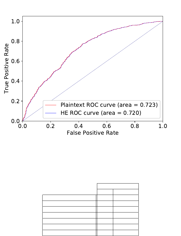
Figure 2 depicts the comparison between the predictions performed in plaintext and homomor-

phically. This is done by means of a ROC curve using a size 2271 sample with known condition to

test against. Both ROC curves are practically indistinguishable, demonstrating that any inaccu-

racies resulting from performing the predictions homomorphically do not signiﬁcantly impact the

quality of the predictions. Table 2 shows performance information including memory usage for the

aforementioned prediction pipeline. Due to the low depth of computation required for performing

a logistic regression prediction operation, our solution achieves acceptable performance even in

the case of 256 bit security. Based on these results, selecting SIG3 provides the solution with the

adequate balance of accuracy and performance.

Fig. 2. ROC curve for plaintext and homomorphic prediction.

Table 2. CPU time and RAM usage of prediction.

Prediction Security

128 bit 256 bit

# Predictions per thread 10745 16530

# Threads 1 1

Encrypted Model size 40 MB 61 MB

Model input time 1 sec 1.3 sec

Encrypted Data size 37 MB 57 MB

Data input time 0.8 sec 1.2 sec

Prediction time 5.4 sec 9.4 sec

Homomorphic variable selection. We performed extensive experimentation in order to deter-

mine the quality of the homomorphic log loss calculations (section 3.4) compared to a fully-plaintext

pipeline which performs similar calculations. In this experimentation, we consider not the log loss

values themselves, but the quality of relative ordering which results from sorting based on these

values. Once an adequate set of parameters were derived for homomorphic log loss calculations,

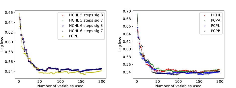
Fig. 3. Log loss for several homomorphic parameters. Fig. 4. Log loss for HE and plain.

we compared the results with various diﬀerent plaintext-based orderings, namely ordering by AUC

and by AP.

Our method for evaluating the quality of the selected ordering was as follows. We took the ﬁrst k

variables ordered by score, then used only these k variables to create a penalized logistic regression

model. We then evaluated the quality of the resultant model using 10-fold cross-validation to derive

a value for the typical scores: AUC, AP, and log loss. This procedure was carried out for each k

between 1 and 200. The results were then plotted on a scatter to evaluate any trends of diﬀering

performance.

The convention used for the curves with four-letter labels (e.g. HCHL) in the graphs below is

the following. The ﬁrst two letters indicate how the variable selection was computed; either HC

or PC for homomorphically computed or plaintext computed, respectively. The third letter H or

P indicate how ordering score was calculated, namely, homomorphically or in the plain. The last

letter indicates which metric was used for ordering (computing a score). This letter can take L, A

or P for ordering by log loss, AUC, or AP, respectively. Thus in combination, the last two letters

should be read as how the variable ordering was performed, e.g. HL for homomorphic log loss or

PL for plaintext log loss.

The ﬁrst step in our assessment was to compare how homomorphic variable selection by logistic

regression ordered by homomorphic log loss (HCHL) really compares with the plaintext version

of variable selection by logistic regression ordered by plaintext-computed log loss (PCPL). This

comparison is illustrated in ﬁgure 3. Furthermore, we compared variations of the diﬀerent HCHL

conﬁgurations, as described in section 4.2. The ﬁgure shows the comparison between diﬀerent

numbers of Nesterov steps and diﬀerent degrees of sigmoid approximations, alongside PCPL as a

baseline for comparison. It is clearly shown that ordering by log loss homomorphically is compa-

rable to computing it in the plain. We can also see that the HCHL conﬁgurations have negligible

diﬀerence. This is signiﬁcant because of the consequences of requiring a higher depth of computa-

tion; namely its considerable eﬀect on computation time and the adverse impact that the requisite

increase in qbits has on security. Nonetheless, for all remaining evaluations, we used the degree-7

sigmoid and 6 Nesterov steps.

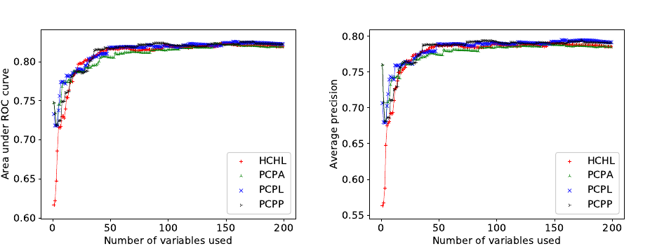
Fig. 5. Evaluation by AUC. Fig. 6. Evaluation by average precision.

Contemporary metrics commonly used for evaluation are AUC and AP. As discussed in ap-

pendix A, these are considered computationally heavy to implement homomorphically. However,

we compare the performance of ordering with these metrics in plaintext only. This comparison is

performed by measuring against all three of the aforementioned evaluation scoring methods. Eval-

uation by log loss can be seen in ﬁgure 4, AUC in ﬁgure 5, and AP in ﬁgure 6. All three of these

ﬁgures support the same conclusion: there is not signiﬁcant diﬀerence between the diﬀerent methods

of ordering, including the homomorphic methodology. One can read from any of the ﬁgures that

by around the time the 50 best-scoring variables have been included the model quality stabilizes at

around the same level.

Table 3 depicts the performance of the homomorphic variable selection with log loss ordering

comparing 5 and 6 Nesterov steps with degree-3 sigmoid approximation. These were run with the

algebras given in table 1. The 6 step version requires deeper computation, thus requiring an algebra

with a larger value for qbits. Consequently the ciphertexts are larger resulting in higher memory

usage than the 5 steps version. In both cases, increasing the number of threads decreases the running

time. However, in the shared and multi-tenant environment we observed that using more than 48

threads for computation did not further decrease the running time of the training phase, which is

a deep computation. This behavior is likely caused by memory locality issues resulting from the

large ciphertexts required. Since there is negligible diﬀerence in the quality of the results for 5 and

6 Nesterov steps as seen in ﬁgure 3, we choose 5 steps as a good compromise between memory

usage, performance, and quality of the results.

5 Conclusion

To progress towards a real-world ML pipeline, we investigated two common pipeline tasks. These

tasks need to be further considered when assessing if HE can be utilized to address whether data

can be aggregated. We have demonstrated that predictions can be performed in a typical business

setting with a powerful architecture in a reasonable amount of time for realistic workloads using

real ﬁnancial data.

Table 3. CPU time and RAM usage of the degree-3 sigmoid with 5-6 Nesterov iterations vs. number of threads.

# Nesterov Data input # Threads Data input Training LogLoss RAM

iterations ciphertext time time time usage

5 64 GB

64 30 s 6062 s 217 s 228 GB

48 37 s 6000 s 205 s 220 GB

32 47 s 6186 s 231 s 217 GB

24 62 s 6467 s 280 s 210 GB

16 92 s 7255 s 388 s 206 GB

8 180 s 9491 s 784 s 200 GB

6 80 GB

64 32 s 9584 s 295 s 284 GB

48 58 s 9481 s 273 s 271 GB

32 58 s 9658 s 303 s 260 GB

24 75 s 9920 s 349 s 257 GB

16 113 s 11349 s 502 s 252 GB

8 218 s 15119 s 987 s 243 GB

Note: The timings in this table are for reference only as the HE code implementation was focused on achieving

numerical ﬁdelity and adequate security.

Prediction on the encrypted reference model took less than 10 seconds with a security level of

256 bits. It was shown that over 16500 predictions can be performed in this time. Variable selection,

while preserving the privacy and conﬁdentiality of the input data, took 1 hour and 43 minutes to

perform for a security level above 128 bits, which is adequate considering that most training tasks

run as batch processes. To achieve these levels of security, we used algebras not previously used

in related work [2] with m = 2

allowing for variable selection to be performed for the depth

required. The CKKS scheme has demonstrated to be invaluable to achieving good accuracy despite

its approximate nature, and with HElib it is now possible to have high accuracy by having the r

parameter set as high as 50.

Moreover, we have shown through comparison that log loss is an adequate metric for ordering

during the homomorphic variable selection. The experimentation demonstrated comparable results

to ordering by common ML metrics such as AUC or AP. This is a good result as log loss is considered

to be of low depth computationally as opposed to homomorphically calculating the other metrics.

6 Further Work

Due to time constraints, we were not able to explore performing the decorrelation homomorphically.

This would be of interest and the next logical step to attempt to tie together a more complete

machine learning pipeline. This might involve homomorphic calculations of correlation coeﬃcients

such as the Pearson correlation coeﬃcient used in this work, then elimination of variables with a

suﬃciently high correlation. At the time of writing, the authors are unaware of any works which

attempt to achieve this and any such scheme would certainly push the depth of computation beyond

what this work performed.

Other future works may include attempting to calculate other model scores such as AUC or

AP in a novel homomorphic way, the latter of which might be of particular interest for heavily

imbalanced datasets. However, the homomorphic application of various threshold values may prove

problematic and high-depth in the absence of any innovative scheme for eﬃciently doing so.

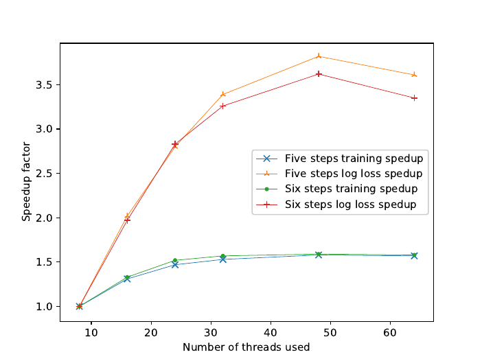
Fig. 7. Computation speed-up of training and log loss versus the number of threads.

It is reasonable to expect that more complete ML pipelines would require higher depth of

computation thus necessitating the requirement for bootstrapping. This would need to be taken

into consideration in implementation.

Acknowledgements

This research was part of the collaboration between IBM Research and Banco Bradesco SA to in-

vestigate the feasibility of utilizing homomorphic encryption technology to protect and preserve the

privacy and conﬁdentiality of ﬁnancial data utilized in machine learning based predictive modeling.

The views and conclusions contained in this document are those of the authors and should not be

interpreted as representing the oﬃcial policies, either expressed or implied, of Banco Bradesco SA.

References

1. Archer, D., Chen, L., Cheon, J.H., Gilad-Bachrach, R., Hallman, R.A., Huang, Z., Jiang, X., Kumaresan, R.,

Malin, B.A., Soﬁa, H., Song, Y., Wang, S.: Applications of homomorphic encryption. Tech. rep., Homomorphi-

cEncryption.org (July 2017)

2. Bergamaschi, F., Halevi, S., Halevi, T.T., Hunt, H.: Homomorphic training of 30, 000 logistic regression models.

In: Applied Cryptography and Network Security - 17th International Conference, ACNS 2019, Bogota, Colombia,

June 5-7, 2019, Proceedings. pp. 592–611 (2019)

3. Blatt, M., Gusev, A., Polyakov, Y., Rohloﬀ, K., Vaikuntanathan, V.: Optimized homomorphic encryption solution

for secure genome-wide association studies. IACR Cryptology ePrint Archive 2019, 223 (2019)

4. Bonte, C., Vercauteren, F.: Privacy-preserving logistic regression training. BMC Medical Genomics 11((Suppl

4)) (2018)

5. Brakerski, Z., Gentry, C., Vaikuntanathan, V.: (leveled) fully homomorphic encryption without bootstrapping.

ACM Transactions on Computation Theory 6(3), 13:1–13:36 (2014)

6. Brutzkus, A., Gilad-Bachrach, R., Elisha, O.: Low latency privacy preserving inference. In: Proceedings of the

36th International Conference on Machine Learning, ICML 2019, 9-15 June 2019, Long Beach, California, USA.

pp. 812–821 (2019)

7. Bubeck, S.: ORF523: Nesterov’s accelerated gradient descent. https://blogs.princeton.edu/imabandit/2013/

04/01/acceleratedgradientdescent, accessed January 2019 (2013)

8. Chen, H., Gilad-Bachrach, R., Han, K., Huang, Z., Jalali, A., Laine, K., Lauter, K.: Logistic regression over

encrypted data from fully homomorphic encryption. BMC Medical Genomics 11((Suppl 4)) (2018)

9. Cheon, J.H., Kim, A., Kim, M., Song, Y.S.: Homomorphic encryption for arithmetic of approximate numbers. In:

Advances in Cryptology - ASIACRYPT 2017 - 23rd International Conference on the Theory and Applications of

Cryptology and Information Security, Hong Kong, China, December 3-7, 2017, Proceedings, Part I. pp. 409–437

(2017)

10. Crawford, J.L.H., Gentry, C., Halevi, S., Platt, D., Shoup, V.: Doing real work with FHE: the case of logistic re-

gression. In: Proceedings of the 6th Workshop on Encrypted Computing & Applied Homomorphic Cryptography,

WAHC@CCS 2018, Toronto, ON, Canada, October 19, 2018. pp. 1–12 (2018)

11. Davis, J., Goadrich, M.: The relationship between precision-recall and ROC curves. In: Machine Learning, Pro-

ceedings of the Twenty-Third International Conference (ICML 2006), Pittsburgh, Pennsylvania, USA, June 25-29,

2006. pp. 233–240 (2006)

12. Fan, J., Vercauteren, F.: Somewhat practical fully homomorphic encryption. IACR Cryptology ePrint Archive

2012, 144 (2012)

13. Gentry, C.: Fully homomorphic encryption using ideal lattices. In: Proceedings of the 41st Annual ACM Sympo-

sium on Theory of Computing, STOC 2009, Bethesda, MD, USA, May 31 - June 2, 2009. pp. 169–178 (2009)

14. Gilad-Bachrach, R., Dowlin, N., Laine, K., Lauter, K.E., Naehrig, M., Wernsing, J.: Cryptonets: Applying neu-

ral networks to encrypted data with high throughput and accuracy. In: Proceedings of the 33nd International

Conference on Machine Learning, ICML 2016, New York City, NY, USA, June 19-24, 2016. pp. 201–210 (2016)

15. Halevi, S., Shoup, V.: HElib - An Implementation of homomorphic encryption. https://github.com/homenc/

HElib (Accessed August 2019)

16. Han, K., Hong, S., Cheon, J.H., Park, D.: Eﬃcient logistic regression on large encrypted data. IACR Cryptology

ePrint Archive 2018, 662 (2018)

17. Hastie, T., Friedman, J.H., Tibshirani, R.: The Elements of Statistical Learning: Data Mining, Inference, and

Prediction. Springer Series in Statistics, Springer (2001)

18. iDASH: Integrating Data for Analysis, Anonymization and SHaring (iDASH). http://www.humangenomeprivacy.

org

19. James, G., Witten, D., Hastie, T., Tibshirani, R.: An introduction to statistical learning, vol. 112. Springer (2013)

20. Kim, A., Song, Y., Kim, M., Lee, K., Cheon, J.H.: Logistic regression model training based on the approximate

homomorphic encryption. IACR Cryptology ePrint Archive 2018, 254 (2018)

21. Kim, M., Song, Y., Wang, S., Xia, Y., Jiang, X.: Secure logistic regression based on homomorphic encryption:

Design and evaluation. JMIR Med. Inform. 6(2), e19 (2018)

22. King, G., Zeng, L.: Logistic regression in rare events data. Political Analysis 9, 137–163 (2001)

23. Nesterov, Y.: Introductory Lectures on Convex Optimization - A Basic Course, Applied Optimization, vol. 87.

Springer (2004)

24. Provost, F.J., Fawcett, T., Kohavi, R.: The case against accuracy estimation for comparing induction algorithms.

In: Proceedings of the Fifteenth International Conference on Machine Learning (ICML 1998), Madison, Wisconsin,

USA, July 24-27, 1998. pp. 445–453 (1998)

25. Samuel, A.L.: Some studies in machine learning using the game of checkers. IBM Journal of Research and

Development 3(3), 210–229 (1959)

26. Su, W., Yuan, Y., Zhu, M.: A relationship between the average precision and the area under the ROC curve.

In: Proceedings of the 2015 International Conference on The Theory of Information Retrieval, ICTIR 2015,

Northampton, Massachusetts, USA, September 27-30, 2015. pp. 349–352 (2015)

27. Zweig, M.H., Campbell, G.: Receiver-operating characteristic (roc) plots: a fundamental evaluation tool in clinical

medicine. Clinical Chemistry 39(4), 561–577 (1993)

Appendix A Model Evaluation Metrics

In section 3.4, we introduced and selected log loss as the metric for the ordering as it is a relatively

simple-to-compute measure that can be calculated homomorphically. To demonstrate its beneﬁts

as a good common metric, we compared log loss to two other common metrics used to evaluate

machine learning models.

Area under curve. The receiver operating characteristic (ROC) curve is a standard tool in eval-

uating the performance of predictive models. The ROC space is typically deﬁned as [0, 1]

where

a point (a, b) ∈ [0, 1]

has the false positive rate a and the true positive rate b of a given set of

binary predictions. For a set of probability predictions, it is typical to trace out the curve in the

ROC space parameterized by a threshold value. Attributes of the ROC curve, including the area

under the curve (AUC) are considered to be superior measures of the quality of a set of predictions

compared to a single accuracy value [27,24].

Average precision. Precision-recall (PR) curves are another tool similar in use to ROC curves,

but are more frequently used in information retrieval or situations in which the two classes are

imbalanced in the dataset. With PR curves, a similar parameterization on threshold value is per-

formed, but the points in [0, 1]

are (precision, recall) pairs instead of (false positive rate, true

positive rate) pairs. The method of taking the area under this curve as a metric, known as the

average precision (AP), is also a common practice. PR and ROC curves have been shown to have

strong links to each other for a given predictor [11] as well as a direct relationship shown by Su et

al. [26] between the AP and AUC scores.

In this work, we experimented with using AUC, AP, and log loss for selecting models and

evaluating quality of derived models. However, we do not compute AUC or AP homomorphically for

the purpose of variable ordering as this would require the application of a large number of threshold

function approximations; likely requiring an extremely high-depth computation in comparison to

our fourth-order log loss approximation in equation (4).