NBER WORKING PAPER SERIES
PARDONS, EXECUTIONS AND HOMICIDE
H. Naci Mocan
R. Kaj Gittings
Working Paper 8639
http://www.nber.org/papers/w8639
NATIONAL BUREAU OF ECONOMIC RESEARCH
1050 Massachusetts Avenue
Cambridge, MA 02138
December
2001
We thank Steve Levitt, Jeff Zax, Woody Eckard for helpful suggestions, and Michael Grossman and Sara
Markowitz for providing us with the alcohol consumption data. The views expressed herein are those of the
authors and not necessarily those of the National Bureau of Economic Research.
© 2001 by H. Naci Mocan R. Kaj Gittings. All rights reserved. Short sections of text, not to exceed two
paragraphs, may be quoted without explicit permission provided that full credit, including © notice, is given
to the source.

Pardons, Executions and Homicide
H. Naci Mocan R. Kaj Gittings
NBER Working Paper No. 8639
December 2001
JEL No. K4, H7
ABSTRACT
This paper uses a data set that consists of the entire history of 6,143 death sentences between
1977 and 1997 in the United States to investigate the impact of capital punishment on homicide. This
data set is merged with state panels that include crime and deterrence measures as well as state
characteristics to analyze the impact of executions and governors’ pardons on criminal activity. Because
the exact month and year of each execution and pardon can be identified, they are matched with criminal
activity in the relevant time frame. Controlling for a variety of state characteristics, the paper investigates
the impact of the execution rate, pardon rate, homicide arrest rate, the imprisonment rate and the prison
death rate on the rate of homicide. The models are estimated in a number of different forms, controlling
for state fixed effects, common time trends, and state-specific time trends. Each additional execution
decreases homicides by 5 to 6, while three additional pardons generate one to 1.5 additional homicides.
These results are robust to model specifications and measurement of the variables.
H. Naci Mocan R. Kaj Gittings
Department of Economics Department of Economics
University of Colorado at Denver University of Colorado at Denver
Campus Box 181, P.O. Box 173364 Campus Box 181, P.O. Box 173364
Denver, CO 80217-3364 Denver, CO 80217-3364
and NBER Tel: 303-556-4934
Tel: 303-556-8540 Email: r[email protected].edu
Email: [email protected].edu

1
“I have inquired for most of my adult life about studies that might show that
the death penalty is a deterrent, and I have not seen any research that would
substantiate that point.”
Former U. S. Attorney General Janet Reno at a Justice Department Press
Briefing; January 20, 2000.
I. Introduction
Empirical studies of the economics of crime have established credible evidence
regarding the impact of sanctions on criminal activity. In particular, it has been
demonstrated that increased arrests and police have deterrent effects on crime (Corman
and Mocan 2000, Levitt 1997, Grogger 1991). The analysis of the determinants of
homicide is especially important because it poses an interesting test for economic theory.
According to the standard economic model of crime, a rational offender would respond to
perceived costs and benefits of committing crime. Murder is an important case to test
this behavioral hypothesis because murder may be considered a crime which can be
committed without regard to costs or benefits of the action. However, empirical tests
reveal that even murder responds to costs of crime. For example, Corman and Mocan
(2000) show that an increase in murder arrests decreases murders in New York City.
Capital punishment is particularly significant in this context, because it represents a very
high cost for committing murder (loss of life). Thus, the presence of capital punishment
in a state, or the frequency with which it is used should unequivocally deter homicide.
Yet, it has been a difficult empirical task to identify the impact of capital punishment on
homicide simply because there is not much variation in the execution rates across states
or over time to estimate its impact on homicide with precision.

2
The statement of former U.S. Attorney General Janet Reno cited above highlights
the mixed scientific evidence on the deterrent effect of the death penalty. Ehrlich (1975)
and Ehrlich (1977a) found a significant deterrent effect of capital punishment on murder
rates using aggregate time series, and cross-sectional data, respectively. Ehrlich’s
findings were challenged by subsequent work (Leamer 1983; Hoenack and Weiler 1980;
Passell and Taylor 1977; Bowers and Pierce 1975) based on the identification of the
murder supply equation, functional form of the equations estimated, the sample period
investigated and the choice of variables. Ehrlich and others responded to these criticisms
(Ehrlich and Liu 1999; Ehrlich and Brower 1987; Ehrlich 1977b). Nevertheless, the
issue of whether the death penalty deters murder is still debated in the media,
1
as well as
in academia (Sorensen et al. 1999; Cameron 1994; Cover and Thistle 1988; McManus
1985; McFarland 1983; Layson 1983; Forst 1983).
Because of the ethical, moral and religious aspects of capital punishment,
executing death row inmates generates repercussions, even from outside the United
States. For example, Pope John Paul II appealed to then-Governor George W. Bush to
stop an execution scheduled for January, 2000. Recently, state lawmakers have been
reacting to the sentiment that there is arbitrariness and possibly a racial bias in the
implementation of the death penalty by proposing legislation to either abolish it, or
1 Recent examples are: CNN Live Today, June 27, 2001, “Gallup Poll: Americans and the Death
Penalty;” Meet the Press, NBC, June 10, 2001 hosting former New York Governor Mario
Cuomo and Oklahoma Governor Frank Keating; The O’Reilly Factor on Fox New Network,
June 11, 2001, “Death Penalty as a Deterrent.”

3
instate a moratorium.
2
Similarly, a bill was introduced in United States Congress
recently to abolish the death penalty under Federal law.
3
In this paper we investigate whether the death penalty is a deterrent for homicide.
An inherent difficulty in uncovering an impact of deterrence on crime is to find
appropriate data sets to overcome the issue of simultaneity between criminal activity and
deterrence measures. Low-frequency time series data or cross-sectional data are not
satisfactory to address the issue (Corman and Mocan 2000, Levitt 1997). We use a state-
level panel data set that contains information on homicide and other crimes, deterrence
variables, relevant capital punishment measures along with a number of state
characteristics. Katz, Levitt and Shustorovich (2001) perform a similar analysis which
focuses on the impact of prison conditions on criminal activity. Differences between this
paper and theirs are highlighted in Section VI.
An innovation of this paper is the use of a Department of Justice data set, which
is new to the literature. This data set contains detailed information on the entire 6,143
deaths sentences between 1977 and 1997 in the United States. For example, the exact
month of removal from death row is identified for each prisoner. This information is
valuable as it allows us to link executions to criminal activity in the proper time frame.
More specifically, previous studies linked the crime rate in a given year to the number of
executions in the same year. However, if an execution takes place towards the end of a
2 Legislators in at least 21 states have recently proposed legislation to modify their current capital
punishment laws. Illinois imposed a moratorium in 2000.

4
year, it cannot considerably effect crime rates in that same year (as the number of crimes
for that year have been committed since January). Rather, such an execution is expected
to impact the crime rate of the following year. This issue is potentially significant
because 47.2 percent of all executions and 50.9 percent of all commutations (pardons of
the death row inmates by the governor) between 1977 and 1997 took place between the
months of July and December. This means that if executions and homicide rates in a
state are not linked in the proper time frame, the estimated coefficient of the execution
rate may be biased toward zero because of this measurement error.
Another innovation of this paper is to investigate the impact of clemency on
homicide. The governor of the state has the power to pardon a prisoner on death row.
According to economic theory, such an action represents a decrease in the cost of
committing the crime, and should have a positive impact on the homicide rate. The
impact of pardons on homicide or other crimes has not been investigated before.
We find a statistically significant relationship between executions, pardons and
homicide. Specifically, each additional execution reduces homicides by 5 to 6, and three
additional pardons generate 1 to 1.5 additional murders.
Section II gives the background on death penalty in the United States. Sections
III and IV describe the methodology and the data, respectively. Section V presents the
results. Section VI consists of the extensions, and Section VII is the conclusion.
3 Federal Death Penalty Abolition Act of 2001, introduced by Senator Russell Feingold; January
25, 2001, S191.

5
II. Recent History of Capital Punishment and the Data Set
In the late 1960s 40 states had laws authorizing use of the death penalty in the
United Sates. However, strong pressure by those opposed to capital punishment resulted
in few executions. For example, there were 145 executions between 1960 and 1962. In
1963 and 1964 there were 21 and 15 executions, respectively. Between 1965 and 1967
there were a total of 10 executions, and nobody was executed between 1968 and 1972.
All executions were halted and hundreds of inmates had their death sentences lifted by a
Supreme Court decision in 1972. In Furman v. Georgia, 408 U.S. 153 (1972) the
Supreme Court struck down federal and state laws that had allowed wide discretion
resulting in arbitrary and capricious application of the death penalty. Three of the
Supreme Court justices voiced concerns that included an appearance of racial bias against
black defendants. Furthermore, laws that imposed a mandatory death penalty and those
that allowed no judicial or jury discretion beyond the determination of guilt were
declared unconstitutional in 1976 [Woodson v. North Carolina, 428 U.S. 280 (1976),
Roberts v. Louisiana, 428 U.S. 325 (1976)].
Starting in the mid-1970s, many states reacted by adopting new legislation to
address the concerns of the Supreme Court, and these new state laws were later upheld by
the Supreme Court [e.g. Gregg v. Georgia, 428 U.S. 153 (1976), Jurek v. Texas, 428 U.S.
262 (1976), and Proffitt v. Florida, 428 U.S. 242 (1976)]. New state statutes created two-
stage trials for capital cases, where guilt/innocence and the sentence were determined in
two different stages. The first post-Gregg execution took place in 1977 in Utah, and the
number of executions has since continued to rise. Currently, only 12 states and the

6
District of Columbia do not have capital punishment, although a number of states
consider abolishing death penalty.
4
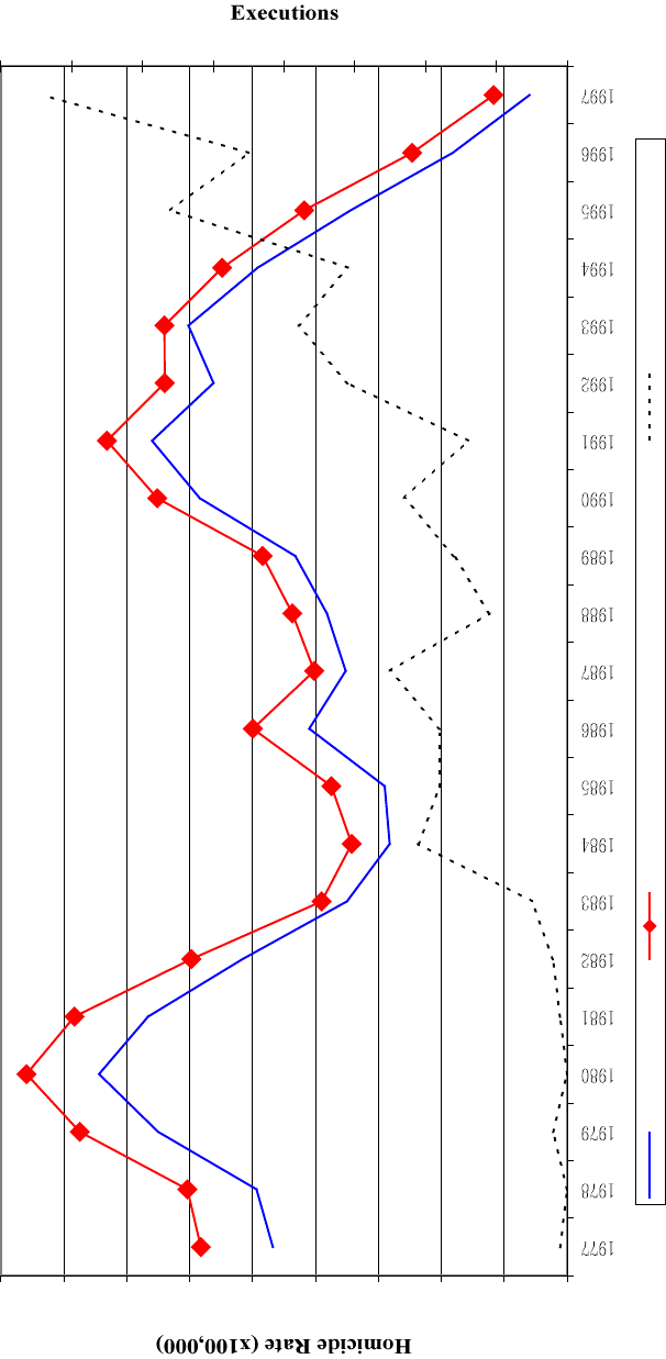
Figure 1 displays the murder rate in the United Sates per 100,000 people between
1977 and 1997, along with the number of executions during the same time period. Also
presented in Figure 1 is the murder rate in states where the death penalty was legal.
Following the first post-Gregg execution in 1977, the number of executions increased to
an average of about 20 per year around mid-1980s. After remaining stable until the early
1990s, the number of executions started rising in 1993, reaching 74 executions in 1997.
The homicide rate in the U.S. was 8.8 murders per 100,000 people in 1977. It reached
10.2 in 1980, and then started declining continuously until 1984. When the number of
executions was relatively stable in late 1980s, the murder rate rose again, reaching 9.8
murders per 100,000 people in 1991. It began declining after 1991 and went down 6.8 in
1997.
III. Empirical methodology
To investigate the impact of capital punishment and other forms of deterrence on
homicide, we estimate regressions of the following form:
(1) MURDER
it
= DETER
it-1
β
ββ
β + X
it
Ω
ΩΩ
Ω +µ
i
+η
t
+ε
it,
where MURDER
it
is the homicide rate in state i and year t, and DETER stands
for the vector of deterrence variables. Following Ehrlich (1975) and the literature that
4
The twelve states are Alaska, Hawaii, Iowa, Maine, Massachusetts, Michigan, Minnesota, North
Dakota, Rhode Island, Vermont, West Virginia and Wisconsin.
7
follows, DETER consists of the subjective probabilities (for potential offenders) that
offenders are apprehended, convicted and executed. The first one of these probabilities is
measured by the murder arrest rate (the proportion of murders cleared by an arrest).
Following Levitt (1998), and Katz, Levitt and Shustorovich (2001), the second
probability is calculated as the number of prisoners per violent crime. As Levitt (1998)
notes, the number of individuals in custody as a fraction of population may correspond
more closely to the theoretical notion of incapacitation. Thus, as an alternative measure
we also employ the number of prisoners per population. The third variable in DETER
pertains to the probability of execution given conviction. Ehrlich (1975) measured this
variable as the ratio of the number of individuals executed in a year to the number of
individuals convicted in the previous year, under the assumption that there is a one-year
lag between conviction and execution. The data set we employ in this paper (explained
below in detail) consists of the universe of persons who were on death row between 1977
and 1997. Since we know the month and year of the imposition of the death sentence for
each person and his/her execution date, we can calculate the time spent on death row.
The average duration on death row for those who are executed between 1977 and 1997 is
9.31 years. Therefore, using the ratio of executions in year t as a fraction of convictions
in year t-9 would lose almost half of our sample. We calculate the probability of
execution as the number of executions per death row inmates. This measure is more
closely linked to the theoretical risk of execution in comparison to some other measures,
such as executions per prisoners.
8
The data set also contains information on death row inmates who are pardoned by
state governors. An increase in pardons implies a decrease in the probability of execution,
which economic theory predicts should have a positive impact on murder rates. We use
the number of pardons per death row inmates as an (inverse) deterrence measure.
Following Katz, Levitt and Shustorovich (2001), Corman and Mocan (2000), and
Levitt (1998), deterrence variables are lagged once to minimize the impact of
simultaneity between the murder rate and deterrence measures. Because the number of
homicides appear in the numerator of the independent variable and in the denominator of
the arrest rate, measurement error in homicides generates biased estimates. Unlike other
types of crimes, measurement error in the homicide variable is unlikely to be
consequential. Nevertheless, lagging the deterrence measures also helps minimize this
potential bias (Levitt 1998).
The vector X contains state characteristics that may be correlated with criminal
activity. It includes information on the unemployment rate, real per capita income, the
proportion of the state population in the following age groups: 20-34, 35-44, 45-54 and
55 and over, the proportion of the state population in urban areas, the proportion which is
black, the infant mortality rate, and per capita beer consumption in the state. Theoretical
and empirical justification for the inclusion of these variables can be found in Levitt
(1998), and Lott and Mustard (1997). The variable µ
i
represents unobserved state-
specific characteristics that impact the murder rate and η
t
represents year effects. To
control for the impact of the 1995 Oklahoma City bombing, we included a dummy

9
variable, which takes the value of one in Oklahoma in 1995, and zero elsewhere. Most
specifications also include state-specific time-trends.
IV. Data
We use data from Capital Punishment in the United States, 1973-1998, complied
by the Department of Commerce and the Bureau of Census, and published by Bureau of
Justice Statistics of the U.S. Department of Justice. The data set contains information on
the exact month and year of the prisoner’s sentencing, and the month and year when the
prisoner is removed from death row. The removal takes place if the prisoner is executed,
commuted (granted clemency by the governor), died on death row, the capital sentence is
declared unconstitutional, the conviction is affirmed but the sentence is overturned, the
conviction is overturned, or the sentence is overturned for other reasons. These data
provide information on the history of 6,143 death sentences between 1977 and 1997 in
the United States.
5
This data set allows us to create deterrence constructs that are
closely linked to theory. For example, as explained above, economic theory suggests that
the murder rate depends on, among other factors, the risk of execution given the death
sentence. Most previous studies proxied the risk of execution by the ratio of executions
to the number of prisoners or murders committed. A more appropriate measure of
5 During this period, three-hundred and forty-six inmates were sentenced twice, 14 inmates
were sentenced three times, and one individual was sentenced four times. There may be a
variety of reasons for multiple sentencing. For example, a sentence can be overturned on
appeal and then be upheld at a later trial. It is also possible to be pardoned or have the
conviction overturned and then commit murder again and receive a separate death sentence.
10
execution risk, which we employ in this paper, is the ratio of executions to the number of
death row inmates.
Second, we analyze, for the first time in this literature, the impact of clemency on
the homicide rate. An increase in the number of pardons handed to death row inmates by
the governor implies a decrease in the risk of execution. Thus, an increase in the pardon
(clemency or commutation) rate is expected to be positively related to murders.
Third, as mentioned earlier, an advantage of our data set is the availability of the
exact date of each execution and pardon. This information enables us to create execution
and pardon measures that are more consistent with theory. More specifically, if
executions or pardons send signals to potential criminals, then the timing of the signal is
important. For example, an execution which took place in January of 1980 can have an
impact on the homicide rate for the full year. However, if the execution took place in
December 1980, it will have a trivial impact on the 1980 homicide rate. Rather, the
impact of this December execution on murder will be felt in 1981. The distribution of
executions are relatively uniform over the year. An investigation of the 432 executions
that took place between 1977 and 1997 shows that approximately 8 percent took place in
each month. Given this, we created the following algorithm: If an execution took place
within the first three quarters of a year, we attributed that execution to the same year. If
the execution took place in the last quarter of a year (October-December) we attributed
that execution to the following year under the assumption that the relative impact on
murders would be felt in the following year. The same was done for pardons.
11
As a second measure, we prorated the executions and pardons based on the month
in which they occurred. As above, an execution that took place in January 1980 is
expected to impact the state homicide rate for the entire twelve months in 1980.
Therefore we count this execution as a full execution in 1980. By contrast, if an
execution took place in November 1980, it is assumed that its deterrent impact on
homicide is felt during the subsequent 12-month period. Thus, this November execution
counts as 2/12 of an execution for 1980 and 10/12 of an execution for 1981. The same
algorithms are applied for pardons. Although these measures are arguably more accurate,
we investigate the sensitivity of the results to the use of a more traditional measure of the
execution rate later in the paper.
Table 1 presents the descriptive statistics of the data. The top-section of the table
presents information on the homicide rate, homicide arrests, two measures of the
execution and pardon rates as well as custody rates and prison deaths. The lower-section
of the table summarizes the data that captures state characteristics. These are per capita
consumption of malt beverages in the state, the state unemployment rate, real per capita
income, the infant mortality rate in the state, percent of population living in urbanized
areas, percent black, the age distribution of state population and a dichotomous variable
to indicate whether the governor is a republican. The bombing of the Federal Building in
Oklahoma City in 1995 is controlled for with the dummy variable Oklahoma City-1995,
although its omission from the models has no impact on the empirical results. The
sources of these data are described in the Appendix.

12
Table 1 also displays the means and standard deviation of the variables in the
sample along with standard deviations of the variables after removing state fixed-effects
and time effects (the middle column) and state fixed-effects, time effects and state-
specific time trends (the right-most column). The variation goes down significantly for
some variables such as Urbanization, Percent Black and age distribution, but substantial
variation remains for most variables.
V. Results
Table 2A displays the regressions where the homicide rate is explained by the
probability of arrest (the number of murder arrests divided by the number of murders),
the custody rate (the number of prisoners per violent crime, or number of prisoners per
population), the risk of execution (the number of executions divided by the number of
death-row inmates), and a number of state characteristics. Following the results of Katz,
Levitt and Shustovich (2001) we also included the prison death rate as a measure of
prison conditions.
Four specifications are presented in the table, all of which contain state fixed-
effects to control for state-specific characteristics that are not captured by the control
variables. All models also include time dummies. Thus, these specifications consider
within-state changes and eliminate the impact of time-invariant omitted factors that are
correlated with deterrence variables across states; while time dummies control for the
unobserved time-varying determinants of homicide which impact all states in the same
13
fashion. Columns 2 and 4 include state-specific time trends to capture the factors that
impact the time-series behavior of homicide which can be different from state to state.
In columns 1 and 2 of Table 2A we present the models where incapacitation is
measured as prisoners per violent crime, and columns 3 and 4 present the models where it
is measured by prisoners per population. Deterrence variables are lagged once and the
models are estimated with weighted-least squares, where the weights are state’s share in
the U.S. population. Robust standard errors are reported in parentheses.
In all specifications, the execution rate is negative and statistically significant,
indicating that an increase in the risk of execution lowers the homicide rate. The same is
true for the custody rates. The prison death rate and the arrest rate have negative
coefficients, but they are not significantly different from zero.
Table 2B is organized similarly, but it reports the results of the model with
Execution Rate-2, which is the pro-rated execution variable (see Section IV for the
description). The results are similar to those reported in Table 2A, as the execution rate
has a negative and statistically significant impact on the homicide rate. Tables 2A and
2B indicate that states with higher infant mortality have higher homicide rates, and an
increase in the share of the population which is 20 to 34 years of age has a positive
impact on the homicide rate. Controlling for state income, an increase in the
unemployment rate is related to a reduction in homicide. This result, which is not
intuitive, is consistent with those reported by Katz, Levitt and Shustorovich (2001),
Ruhm (2001, 2000), and Raphael and Winter-Ebmer (2001).
14
Tables 3A and 3B present the results where the risk of execution is replaced by
the probability of being pardoned by the governor. Theory suggests that an increase in
pardons represents a decrease in deterrence, and therefore should increase the propensity
to commit murder. Although there are only 123 pardons between 1977 and 1997, this
variable is estimated with surprising precision. The pardon rate is positive and
significantly different from zero in both tables, indicating that an increase in pardons
generates an increase in the homicide rate. The impact of other variables are consistent
with those reported in Tables 2A and 2B.
In tables 4A and 4B we present models where the risk of execution and the
probability of pardon are included jointly. The structure of these tables is similar to
Tables 2A-3B. Table 4A reports the results with the first measure of the execution and
pardon rates, and Table 4B displays the results obtained from the second measure. As
before, each table summarizes the results with two different custody rates (prisoners per
violent crime and prisoners per population). The deterrence variables have predicted
signs. Custody variables have a negative impact on the homicide rate. Although
homicide arrests and prison deaths have negative coefficients, they are not significantly
different from zero. Both execution and pardon variables are significant. An increase in
executions decreases the murder rate, and an increase in pardons increases it. The
magnitude of the impact of an execution is surprisingly similar to that reported by Ehrlich
(1975). Each additional execution results in a reduction of murders by 5 to 6. The
impact of pardons is smaller. Three additional pardons yield between 1 and 1.5
additional homicides.
15
In Table 5 we report the results of the models where the deterrence variables enter
with three lags to allow richer dynamics. Put differently, the homicide rate in year t is
impacted by the execution rate, pardon rate, arrest rate, custody rate and prison death rate
in years t-1, t-2 and t-3. The models include state fixed effects, time dummies and state
trends. The results are consistent with previous tables. With very few exceptions, the
individual coefficients of deterrence variables have expected signs: the coefficients of
executions, arrests, custody and prison deaths are negative, and those of pardons are
positive. Table 5 also reports the sum of the lags for the deterrence variables along with a
test for statistical significance of the sums. For example, the sum of three lags of the
execution rate is always significant, ranging from –0.07 to
–0.10. The sum of pardon rate lags is approximately 0.02 and it is significant in all four
specifications. The sums of custody lags is negative and significantly different from
zero, while the sum of prison death rate lags and the sum of arrest rate lags are not
significant. The signs and significance levels of other control variables are similar to
those reported in earlier tables.
To investigate whether the presence of the death penalty has a direct impact on
the homicide rate, we added a dichotomous variable to the models which takes the value
of one if capital punishment is legal in the state and zero otherwise. The existence of the
death penalty in a state is unlikely to be an exogenous event; rather it may be influenced
by the murder rate. To avoid this simultaneity, we lagged the dichotomous variable by
one year. The result is presented in column I of Table 6. The models include state and
year dummies as well as state trends. There is sufficient variation of the dummy variable
16
that measures the legality of the death penalty in a state as seven states legalized the death
penalty between 1977 and 1997 (Kansas, New Hampshire, New Jersey, New Mexico,
New York, Oregon and South Dakota), and Massachusetts and Rhode Island abolished it
during the same time period. The variable (Death Penalty Legal) is negative and
significantly different from zero indicating that the presence of death penalty has a
negative impact on the murder rate. In column two we report the result where Death
Penalty Legal is interacted with the lagged execution and pardon rates. The coefficients
of the execution and pardon rates are negative and positive, respectively; and both are
significant with magnitudes similar to those reported earlier. The coefficient of Legal,
which is the same as the one reported in column 1 suggests that the presence of death
penalty lowers the number of murders by 67.
As an alternative specification, it may be reasonable to assume that the presence
of capital punishment in the state is a function of past homicide rates in the state. More
specifically, consider the following formulation for the existence of capital punishment.
(2) L
t
= MURDER
t-1
+&MURDER
t-2
+&
2
MURDER
t-3
+&
3
MURDER
t-4
+…,
where L
t
represents the death penalty indicator in the state in year t, MURDER stands for
the homicide rate in the state, and & is less than one in absolute value. Equation (2)
portrays the existence of capital punishment in year t as a function of past homicide rates
in the state, where homicide rates in more distant past have smaller impacts. Our main
equation of interest, Equation (1), can be expressed more compactly as
(3) MURDER
t
=
β DETER
t-1
+ε
t,

17
where state subscripts and other determinants of homicide are suppressed for ease of
exposition. Substituting (3) into (2) gives
(4) L
t
= β DETER
t-2
+β&DETER
t-3
+β&
2
DETER
t-4
+β&
3
DETER
t-5
+…,
It is straightforward to show that Equation (4) can be re-written as
(5) L
t
= β DETER
t-2
+&L
t-1
Equation (5) suggests that the presence of capital punishment, although
endogenous, can be instrumented with twice-lagged deterrence variables and lagged
capital punishment law. The results of the instrumental variables estimation are
presented in column 3 of Table 6. Again, the coefficient of the death penalty indicator
(Death Penalty Legal) is negative and statistically significant. The magnitude of the
coefficient implies that the presence of the capital punishment in the state is associated
with a reduction of 95 homicides in this specification. Once again, this effect does not
influence the coefficient of the execution rate, which indicates that an additional
execution generates a reduction in homicide by a magnitude of 6. The coefficient of the
pardon rate gets slightly larger in this specification, indicating that each new pardon
generates one new homicide. The coefficients of other deterrence variables are also
consistent with those reported in previous tables.
VI. Extensions
To investigate the nonlinear impacts of executions and pardons on homicide, we
estimated the models by adding squared terms of the lagged execution and pardon rates.
18
The coefficient of the lagged execution rate was negative and significant at the nine
percent level, while its squared term was positive but insignificant. Similarly, the pardon
rate was positive and significant at the nine percent level, while its squared term was
negative but not significantly different from zero.
We also estimated the models in the logarithms of the murder rate. The results,
which are reported in tables APP-1A and APP-1B in the appendix are consistent with the
ones reported earlier where the homicide rate was in levels.
Katz, Levitt and Shustorovich (2001) estimated separate models that included
region-year and state-decade interactions. As explained in their paper, inclusion of
region-year interactions allows the parameters of the model to be identified off of
differences across states within a particular region and year. For this exercise we
classified the states into four regions: Northeast, Midwest, South and West. Inclusion of
state-decade interactions implies that we exploit the variation within a state around that
state’s mean value in a particular decade. Since our data starts in 1977, we split the
sample into two periods: 1990s and the rest of the sample. These results are reported in
APP-2A and APP-2B in the Appendix. Table APP-2A presents the results of the models
with the first measure of the execution and pardon rates. Columns I and II are models
with state-decade interactions, and columns III and IV are models with region-year
interactions. The first and third columns include prisoners per violent crime as a measure
of custody, and columns II and IV use prisoners per population as a measure of custody.
The results are consistent with earlier tables, but the execution rate is estimated with
smaller precision in specifications with region-year interactions. Table APP-2B, which

19
uses our alternative execution and pardon measures (Execution Rate-2, Pardon Rate-2),
reports similar results although the execution rate is not significant at conventional levels.
Katz, Levitt and Shustorovich (2001) find that prison deaths have a negative
impact on crime rates, while the impact of executions is not significant. Although the
methodology of this paper and that of theirs as well as much of the data used are the
same, there are some differences that may account for the dissimilarity in the results.
First, our data covers the post-Gregg time period 1977-1997 while theirs cover 1950-
1990.
6
Another difference between the papers is the measurement of the execution rate.
While we measure the risk of execution as executions per death row inmates, their
measure is executions per prisoners. Finally, their models do not contain murder arrest
rate as an explanatory variable and a few other control variables, while ours do.
To understand how these differences may impact the results, we estimated
models, where the measurement of variables and model specifications are almost
identical to those estimated by Katz, Levitt and Shustorovich (2001). The results are
reported in Table 7. Here, the execution rate is measured as the number of executions in
a year per 1,000 prisoners in the same year. Column I reports the result of the model
which is comparable to the benchmark specification of Katz, Levitt and Shustorovich
(2001). Following their specification, prisoners per violent crime and prisoners per
population are included jointly, and the model does not include the murder arrest rate. In
6 When Katz, Levitt and Shustorovich (2001) estimated their models between 1971 and 1990
the estimated coefficient of the execution rate was negative and not quite significant with a t-
statistics of -1.60.
20
this specification the prison death rate is not statistically significant, whereas the
execution rate and prisoners per violent crime are negative and significant.
Column II displays the same model with one change: the specification now
includes the murder arrest rate. The coefficients and their statistical significance are the
same as in column I. The murder arrest rate has a negative coefficient which is not
significantly different from zero. Column III adds the Oklahoma City dummy and the
Republican Governor dummy to the specification reported in column II, and column IV is
similar to our benchmark specification, which includes one custody variable, rather than
two. Consistent with the rest of the table, the execution rate and prisoners per violent
crime have negative coefficients which are significantly different from zero, while the
arrest rate and the prison death rate are not significant. The coefficients of the execution
rate per 1000 prisoners range from –0.013 to –0.014, which indicates that in this
specification an additional execution reduces homicide by a magnitude of 5 to 6 as
before.
These results suggest that differences in model specification and measurement of
variables are not likely reasons for the differences between our results and those reported
by Katz, Levitt and Shustorovich (2001). It is likely that the time span analyzed drives
the results. In particular, we focus on the period of 1977-1997 which includes a
significant number of executions in comparison to earlier periods. More specifically,
between 1971 and 1976 there were no executions in the United States because of the
actions of the Supreme Court, as described in Section II. There were three executions
between 1977 and 1979, and 140 prisoners were executed between 1980 and 1990. Thus,
21
in the 20 years covering 1971 to 1990 there were a total of 143 executions. On the other
hand, there were more than twice as many executions (312) in a seven-year time span
between 1991 and 1997. Thus, it is possible that the 1990s which is covered by our data
has increased the precision of the estimated impact of capital punishment on homicide.
To investigate how pardons, executions and other deterrence variables impact
crimes other than homicide, we investigated their impact on robberies, burglaries, rapes
and motor-vehicle thefts. To the extent that capital punishment is a murder-specific
deterrent, they are not expected to have significant impact on these crimes. On the other
hand, executions may impact violent crimes such robbery and rape if the offender is
aware of the possibility that a robbery or rape may end up as a homicide. Alternatively,
an execution may have a negative impact on all crimes if it provides a signal to potential
offenders regarding the attitude of the criminal justice system and that of the governor.
Along the same lines, a pardon by the governor may be taken as a signal for a more
lenient criminal justice environment and therefore may promote criminal activity.
Table App-3 presents the results for robbery, burglary, rape and motor-vehicle
theft. For each model, crime-specific arrests are included. An increase in the custody
rate, measured by prisoners per population, lowers all four crimes reported in the table.
An increase in robbery, burglary arrests and rape arrests reduces these crimes, while the
coefficient of motor vehicle arrests is positive. None of these crimes is influenced by the
execution rate or the pardon rate.

22
VII. Conclusion and Discussion
The investigation of whether the death penalty deters homicide is important from
an academic as well a public policy point of view. The effectiveness of capital
punishment as a crime control device and its appropriateness in a modern democratic
society have both been hotly debated in the United States. This paper uses a data set that
consists of the entire history of 6,143 death sentences between 1977 and 1997 in the
United States to investigate the impact of capital punishment on homicide. We merge
this data set with state panels that include crime and deterrence measures as well as state
characteristics. Our data set allows us not only to analyze the impact of executions, but
also for the first time in the literature, the impact of pardons by governors on criminal
activity. Because we can identify the exact month and year of each execution and
pardon, we can match them with criminal activity in the relevant time frame. Controlling
for a variety of state characteristics, we investigate the impact of the execution rate,
pardon rate, homicide arrest rate, the imprisonment rate and the prison death rate on the
rate of homicide. The models are estimated in a number of different forms, controlling for
state fixed effects, common time trends, and state-specific time trends. We find a
significant relationship between the execution and pardon rates and the rate of homicide.
Each additional execution decreases homicides by 5 to 6, while three additional pardons
generate one to 1.5 additional homicides. These results are very robust to model
specifications and measurement of the variables.
Although these results demonstrate the existence of the deterrent effect of capital
punishment, it should be noted that there remains a number of significant issues
23
surrounding the imposition of the death penalty. For example, although the Supreme
Court of the United States remains unconvinced that there exists racial discrimination in
the imposition of the death penalty, recent research points to the possibility of such
discrimination (Baldus et al. 1998, Pokorak 1998, Kleck 1981). Along the same lines,
there is evidence indicating that there is discrimination regarding who gets executed and
who gets pardoned once the death penalty is received (Argys and Mocan 2001). Given
these concerns, a stand for or against capital punishment should be taken with caution.
25
Figure 1
The Homicide Rate vs Total Executions in the United States
6.5
7
7.5
8
8.5
9
9.5
10
10.5
11
0
10
20
30
40
50
60
70
80
U.S. Homicide Rate Homicide Rate In States Where Death Penalty Is Legal Total Executions in the U.S.

26
Table 1
Descriptive Statistics of the Data
Full
Sample
Standard Deviation
Variable Description
Mean
(Std.Dev)
Filtering
State and
Time
Effects
Filtering
State, Time
and State
Trends
Homicide Rate The number of homicides divided by the
population, multiplied by 1000.
0.070
(0.038) (0.012) (0.010)
Homicide Arrest Rate The number of homicide arrests divided by
the number of reported homicides.
0.876
(0.312) (0.243) (0.219)
Execution Rate The number of executions in the first three
quarters of the current year and the last
quarter of the previous year, divided by the
number of persons on death row.
0.006
(0.036) (0.034) (0.033)
Execution Rate-2 A prorated count of the number of executions
in the previous and current year divided by
the number of persons on death row.
0.006
(0.035) (0.033) (0.032)
Pardon Rate The number of pardons in the first three
quarters of the current year and the last
quarter of the previous year, divided by the
number of persons on death row.
0.010
(0.175) (0.168) (0.159)
Pardon Rate-2 A prorated count of the number of pardons in
the previous and current year divided by the
number of persons on death row.
0.009
(0.140) (0.135) (0.128)
Prisoners Per
Population
The number of persons in custody of state
correctional authorities divided by the adult
population, multiplied by 1000.
2.755
(1.539) (0.520) (0.274)
Prisoners Per Violent
Crime
The number of persons in custody of state or
federal correctional authorities divided by the
total number of violent crimes.
0.518
(0.288) (0.135) (0.086)
Prison Death Rate The number of prison deaths other than
executions divided by the number of state
prisoners, multiplied by 1000.
2.457
(1.872) (1.700) (1.589)
Alcohol Consumption The per capita consumption of malt beverages
(gallons) in the current year.
23.649
(4.202) (1.312) (0.793)
Unemployment Rate The state unemployment rate. 6.398
(2.084) (1.111) (1.033)
Per Capita Income Real per capita income in 1982-1984 dollars,
divided by 1000.
13.438
(2.322) (0.638) (0.354)
Infant Mortality Rate The number of deaths under 1 year of age per
1000 live births.
10.076
(2.516) (0.953) (0.885)
Urbanization The percent of the state population residing in
urbanized areas.
67.781
(14.467) (0.877) (0.138)

27
(Table 1 Concluded)
Republican Governor Dummy Variable (=1) if the Governor is
Republican in that Year.
0.409
(0.492) (0.408) (0.351)
Percent Black The percent of the state population that is
Black.
9.388
(9.464) (1.420) (1.193)
Percent 20-34 The percent of the state population that is
age 20 to 34.
24.675
(2.406) (0.858) (0.459)
Percent 35-44 The percent of the state population that is
age 35 to 44.
13.866
(2.184) (0.370) (0.233)
Percent 45-54 The percent of the state population that is
age 45 to 54.
10.319
(1.199) (0.312) (0.142)
Percent 55+ The percent of the state population that is
age 55 or older.
20.292
(2.977) (0.539) (0.297)
Oklahoma City 1995 Dummy variable (=1) for Oklahoma in year
1995.
0.001
(0.031) (0.030) (0.028)
n = 1050
Ψ
Ψ We have 1047 observations for the Homicide Arrest Rate and 1049 observations for the Prison Death Rate.

28
Table 2A
The Determinants of the Homicide Rate
(Models with First Execution Rate Measure)
(I) (II) (III) (IV)
Variable
Execution Rate (-1) -0.046*
(0.025)
-0.041*
(0.022)
-0.041*
(0.024)
-0.039*
(0.022)
Homicide Arrest Rate (-1) -0.004
(0.003)
-0.002
(0.002)
-0.004
(0.003)
-0.002
(0.002)
Prisoners Per Violent Crime (-1) -0.03***
(0.008)
-0.045***
(0.006)
__ __
Prisoners Per Population (-1) __ __ -0.007***
(0.001)
-0.007***
(0.001)
Prison Death Rate (-1) -0.0002
(0.0003)
-0.0002
(0.0003)
-0.0001
(0.0003)
0.0003
(0.0003)
Percent Black -0.0006
(0.0004)
-0.0003
(0.0003)
-0.0004
(0.0004)
-0.0003
(0.0003)
Republican Governor -0.001
(0.001)
-0.002*
(0.001)
-0.001
(0.001)
-0.002**
(0.001)
Unemployment Rate -0.001***
(0.001)
-0.002***
(0.001)
-0.002***
(0.001)
-0.002**
(0.001)
Per Capita Income 0.001
(0.001)
0.002
(0.002)
-0.0003
(0.001)
0.003*
(0.002)
Infant Mortality Rate 0.002***
(0.001)
0.001
(0.001)
0.002***
(0.001)
0.001
(0.001)
Urbanization 0.002***
(0.001)
-0.011*
(0.006)
0.002***
(0.001)
-0.013**
(0.006)
Alcohol Consumption -0.001**
(0.001)
-0.001
(0.001)
-0.001*
(0.001)
-0.001
(0.001)
Percent 20-34 0.005***
(0.001)
0.003***
(0.001)
0.006***
(0.001)
0.004***
(0.001)
Percent 35-44 0.004***
(0.002)
-0.001
(0.002)
0.002
(0.002)
-0.0003
(0.002)
Percent 45-54 0.006***
(0.002)
-0.002
(0.003)
0.003*
(0.002)
-0.003
(0.003)
Percent 55+ 0.004***
(0.001)
-0.002
(0.002)
0.002*
(0.001)
-0.002
(0.002)
Oklahoma City 1995 0.053***
(0.004)
0.05***
(0.005)
0.054***
(0.004)
0.052***
(0.005)
Number of Observations 996 996 996 996
R-Squared 0.905 0.944 0.908 0.942
State-Fixed Effects? Yes Yes Yes Yes
Time Dummies? Yes Yes Yes Yes
State Trends? No Yes No Yes
Robust standard errors are in parentheses.
* indicates statistical significance between 10% and 5% ; ** indicates statistical significance between 5% to
1%; *** indicates statistical significance at the 1% level or better.

29
Table 2B
The Determinants of the Homicide Rate
(Models with Second Execution Rate Measure)
(I) (II) (III) (IV)
Variable
Execution Rate-2 (-1) -0.049*
(0.026)
-0.032*
(0.019)
-0.042*
(0.023)
-0.029
(0.019)
Homicide Arrest Rate (-1) -0.004
(0.003)
-0.002
(0.002)
-0.004
(0.003)
-0.002
(0.002)
Prisoners Per Violent Crime (-1) -0.029***
(0.008)
-0.045***
(0.006)
__ __
Prisoners Per Population (-1) __ __ -0.007***
(0.001)
-0.007***
(0.001)
Prison Death Rate (-1) -0.0003
(0.0003)
0.0002
0.0003
-0.0001
(0.0003)
0.0002
(0.0003)
Percent Black -0.0005
(0.0004)
-0.0003
(0.0003)
-0.0004
(0.0004)
-0.0003
(0.0003)
Republican Governor -0.001
(0.001)
-0.002*
(0.001)
-0.001
(0.001)
-0.002**
(0.001)
Unemployment Rate -0.001***
(0.001)
-0.002***
(0.001)
-0.002***
(0.001)
-0.002**
(0.001)
Per Capita Income 0.001
(0.001)
0.003
(0.002)
-0.0003
(0.001)
0.003*
(0.002)
Infant Mortality Rate 0.002***
(0.001)
0.001
(0.001)
0.002***
(0.001)
0.001
(0.001)
Urbanization 0.002***
(0.001)
-0.011*
(0.006)
0.002***
(0.001)
-0.013**
(0.006)
Alcohol Consumption -0.001**
(0.001)
-0.001
(0.001)
-0.001*
(0.001)
-0.001
(0.001)
Percent 20-34 0.005***
(0.001)
0.003***
(0.001)
0.006***
(0.001)
0.004***
(0.001)
Percent 35-44 0.004***
(0.002)
-0.001
(0.002)
0.002
(0.002)
-0.0003
(0.002)
Percent 45-54 0.006***
(0.002)
-0.002
(0.003)
0.003*
(0.002)
-0.003
(0.003)
Percent 55+ 0.004***
(0.001)
-0.002
(0.002)
0.002*
(0.001)
-0.002
(0.002)
Oklahoma City 1995 0.053***
(0.004)
0.05***
(0.005)
0.054***
(0.004)
0.052***
(0.005)
Number of Observations 996 996 996 996
R-Squared 0.905 0.944 0.908 0.942
State-Fixed Effects? Yes Yes Yes Yes
Time Dummies? Yes Yes Yes Yes
State Trends? No Yes No Yes
Robust standard errors are in parentheses.
* indicates statistical significance between 10% and 5% ; ** indicates statistical significance between 5% to
1%; *** indicates statistical significance at the 1% level or better.

30
Table 3A
The Determinants of the Homicide Rate
(Models with First Pardon Rate Measure)
(I) (II) (III) (IV)
Variable
Pardon Rate (-1) 0.003***
(0.001)
0.005***
(0.001)
0.003***
(0.001)
0.005***
(0.001)
Homicide Arrest Rate (-1) -0.004
(0.003)
-0.002
(0.002)
-0.004
(0.003)
-0.002
(0.002)
Prisoners Per Violent Crime (-1) -0.03***
(0.008)
-0.045***
(0.006)
__ __
Prisoners Per Population (-1) __ __ -0.007***
(0.001)
-0.007***
(0.001)
Prison Death Rate (-1) -0.0002
(0.0003)
0.0002
(0.0003)
-0.00003
(0.0003)
0.0003
(0.0003)
Percent Black -0.0006
(0.0004)
-0.0003
(0.0003)
-0.0004
(0.0004)
-0.0003
(0.0003)
Republican Governor -0.001
(0.001)
-0.002*
(0.001)
-0.001
(0.001)
-0.002**
(0.001)
Unemployment Rate -0.001***
(0.001)
-0.002***
(0.001)
-0.002***
(0.001)
-0.002***
(0.001)
Per Capita Income 0.001
(0.001)
0.003
(0.002)
-0.0002
(0.001)
0.003*
(0.002)
Infant Mortality Rate 0.002***
(0.001)
0.001
(0.001)
0.002***
(0.001)
0.001
(0.001)
Urbanization 0.002***
(0.001)
-0.011*
(0.006)
0.002***
(0.001)
-0.013**
(0.006)
Alcohol Consumption -0.001**
(0.001)
-0.001
(0.001)
-0.001*
(0.001)
-0.001
(0.001)
Percent 20-34 0.005***
(0.001)
0.003**
(0.001)
0.006***
(0.001)
0.004***
(0.001)
Percent 35-44 0.004**
(0.002)
-0.001
(0.002)
0.002
(0.002)
-0.00002
(0.002)
Percent 45-54 0.006***
(0.002)
-0.002
(0.003)
0.003
(0.002)
-0.003
(0.003)
Percent 55+ 0.003***
(0.001)
-0.002
(0.002)
0.002*
(0.001)
-0.002
(0.002)
Oklahoma City 1995 0.053***
(0.004)
0.05***
(0.005)
0.054***
(0.004)
0.052***
(0.005)
Number of Observations 996 996 996 996
R-Squared 0.905 0.944 0.908 0.942
State-Fixed Effects? Yes Yes Yes Yes
Time Dummies? Yes Yes Yes Yes
State Trends? No Yes No Yes
Robust standard errors are in parentheses.
* indicates statistical significance between 10% and 5% ; ** indicates statistical significance between 5% to
1%; *** indicates statistical significance at the 1% level or better.

31
Table 3B
The Determinants of the Homicide Rate
(Models with Second Pardon Rate Measure)
(I) (II) (III) (IV)
Variable
Pardon Rate-2 (-1) 0.003**
(0.002)
0.006***
(0.002)
0.004**
(0.002)
0.006***
(0.002)
Homicide Arrest Rate (-1) -0.004
(0.003)
-0.002
(0.002)
-0.004
(0.003)
-0.002
(0.002)
Prisoners Per Violent Crime (-1) -0.03***
(0.008)
-0.045***
(0.006)
__ __
Prisoners Per Population (-1) __ __ -0.007***
(0.001)
-0.007***
(0.001)
Prison Death Rate (-1) -0.0002
(0.0003)
0.0002
(0.0003)
-0.00004
(0.0003)
0.0003
(0.0003)
Percent Black -0.0006
(0.0008)
-0.0003
(0.0003)
-0.0004
(0.0004)
-0.0003
(0.0003)
Republican Governor -0.001
(0.001)
-0.002*
(0.001)
-0.001
(0.001)
-0.002**
(0.001)
Unemployment Rate -0.002***
(0.001)
-0.002***
(0.001)
-0.002***
(0.001)
-0.002***
(0.001)
Per Capita Income 0.001
(0.001)
0.003
(0.002)
-0.0003
(0.001)
0.003*
(0.002)
Infant Mortality Rate 0.002***
(0.001)
0.001
(0.001)
0.002***
(0.001)
0.001
(0.001)
Urbanization 0.002***
(0.001)
-0.011*
(0.006)
0.002***
(0.001)
-0.013**
(0.006)
Alcohol Consumption -0.001**
(0.001)
-0.001
(0.001)
-0.001*
(0.001)
-0.001
(0.001)
Percent 20-34 0.005***
(0.001)
0.003***
(0.001)
0.006***
(0.001)
0.004***
(0.001)
Percent 35-44 0.004**
(0.002)
-0.001
(0.002)
0.002
(0.002)
0.00006
(0.002)
Percent 45-54 0.006***
(0.002)
-0.002
(0.003)
0.003
(0.002)
-0.002
(0.003)
Percent 55+ 0.003**
(0.001)
-0.002
(0.002)
0.002*
(0.001)
-0.002
(0.002)
Oklahoma City 1995 0.053***
(0.004)
0.05***
(0.005)
0.054***
(0.004)
0.052***
(0.005)
Number of Observations 996 996 996 996
R-Squared 0.905 0.946 0.908 0.942
State-Fixed Effects? Yes Yes Yes Yes
Time Dummies? Yes Yes Yes Yes
State Trends? No Yes No Yes
Robust standard errors are in parentheses.
* indicates statistical significance between 10% and 5% ; ** indicates statistical significance between 5% to
1%; *** indicates statistical significance at the 1% level or better.

32
Table 4A
The Determinants of the Homicide Rate
(Models with First Measure of Execution Rate and Pardon Rate)
(I) (II) (III) (IV)
Variable
Execution Rate (-1) -0.045*
(0.024)
-0.041*
(0.022)
-0.039*
(0.023)
-0.039*
(0.022)
Pardon Rate (-1) 0.003***
(0.001)
0.005***
(0.001)
0.003***
(0.001)
0.005***
(0.001)
Homicide Arrest Rate (-1) -0.004
(0.003)
-0.002
(0.002)
-0.004
(0.003)
-0.002
(0.002)
Prisoners Per Violent Crime (-1) -0.029***
(0.008)
-0.045***
(0.006)
__ __
Prisoners Per Population (-1) __ __ -0.007***
(0.001)
-0.007***
(0.001)
Prison Death Rate (-1) -0.0002
(0.0003)
0.0002
(0.0003)
-0.00003
(0.0003)
0.0003
(0.0003)
Percent Black -0.0006
(0.0004)
-0.0003
(0.0003)
-0.0004
(0.0004)
-0.0003
(0.0003)
Republican Governor -0.001
(0.001)
-0.002*
(0.001)
-0.001
(0.001)
-0.002**
(0.001)
Unemployment Rate -0.001***
(0.001)
-0.002***
(0.001)
-0.002***
(0.001)
-0.002***
(0.001)
Per Capita Income 0.001
(0.001)
0.003
(0.002)
-0.0003
(0.001)
0.003*
(0.002)
Infant Mortality Rate 0.002***
(0.001)
0.001
(0.001)
0.002***
(0.001)
0.001
(0.001)
Urbanization 0.002***
(0.001)
-0.011*
(0.006)
0.002***
(0.001)
-0.013**
(0.006)
Alcohol Consumption -0.001**
(0.001)
-0.001
(0.001)
-0.001*
(0.001)
-0.001
(0.001)
Percent 20-34 0.005***
(0.001)
0.003***
(0.001)
0.006***
(0.001)
0.004***
(0.001)
Percent 35-44 0.004***
(0.002)
-0.001
(0.002)
0.002
(0.002)
0.0001
(0.002)
Percent 45-54 0.006***
(0.002)
-0.002
(0.003)
0.003*
(0.002)
-0.003
(0.003)
Percent 55+ 0.003**
(0.001)
-0.002
(0.002)
0.002*
(0.001)
-0.002
(0.002)
Oklahoma City 1995 0.053***
(0.004)
0.05***
(0.005)
0.054***
(0.004)
0.052***
(0.005)
Number of Observations 996 996 996 996
R-Squared 0.905 0.945 0.908 0.943
State-Fixed Effects? Yes Yes Yes Yes
Time Dummies? Yes Yes Yes Yes
State Trends? No Yes No Yes
Robust standard errors are in parentheses.
* indicates statistical significance between 10% and 5% ; ** indicates statistical significance between 5% to
1%; *** indicates statistical significance at the 1% level or better.

33
Table 4B
The Determinants of the Homicide Rate
(Models with Second Measure of Execution Rate and Pardon Rate)
(I) (II) (III) (IV)
Variable
Execution Rate-2 (-1) -0.048*
(0.026)
-0.033*
(0.019)
-0.04*
(0.023)
-0.03
(0.019)
Pardon Rate-2 (-1) 0.003**
(0.002)
0.006***
(0.002)
0.004**
(0.002)
0.007***
(0.002)
Homicide Arrest Rate (-1) -0.004
(0.003)
-0.002
(0.002)
-0.004
(0.003)
-0.002
(0.002)
Prisoners Per Violent Crime (-1) -0.029***
(0.008)
-0.045***
(0.006)
__ __
Prisoners Per Population (-1) __ __ -0.007***
(0.001)
-0.007***
(0.001)
Prison Death Rate (-1) -0.0002
(0.0003)
0.0002
(0.0003)
-0.00004
(0.0003)
0.0003
(0.0003)
Percent Black -0.006
(0.0004)
-0.0003
(0.0003)
-0.0004
(0.0004)
-0.0003
(0.0003)
Republican Governor -0.001
(0.001)
-0.002*
(0.001)
-0.001
(0.001)
-0.002**
(0.001)
Unemployment Rate -0.001***
(0.001)
-0.002***
(0.001)
-0.002***
(0.001)
-0.002***
(0.001)
Per Capita Income 0.001
(0.001)
0.003
(0.002)
-0.0003
(0.001)
0.003*
(0.002)
Infant Mortality Rate 0.002***
(0.001)
0.001
(0.001)
0.002***
(0.001)
0.001
(0.001)
Urbanization 0.002***
(0.001)
-0.011*
(0.006)
0.002***
(0.001)
-0.013**
(0.006)
Alcohol Consumption -0.001**
(0.001)
-0.001
(0.001)
-0.001*
(0.001)
-0.001
(0.001)
Percent 20-34 0.005***
(0.001)
0.003***
(0.001)
0.006***
(0.001)
0.004***
(0.001)
Percent 35-44 0.004***
(0.002)
-0.001
(0.002)
0.002
(0.002)
0.0002
(0.002)
Percent 45-54 0.006***
(0.002)
-0.002
(0.003)
0.003*
(0.002)
-0.003
(0.003)
Percent 55+ 0.003**
(0.001)
-0.002
(0.002)
0.002*
(0.001)
-0.002
(0.002)
Oklahoma City 1995 0.053***
(0.004)
0.05***
(0.005)
0.054***
(0.004)
0.052***
(0.005)
Number of Observations 996 996 996 996
R-Squared 0.905 0.945 0.908 0.942
State-Fixed Effects? Yes Yes Yes Yes
Time Dummies? Yes Yes Yes Yes
State Trends? No Yes No Yes
Robust standard errors are in parentheses.
* indicates statistical significance between 10% and 5% ; ** indicates statistical significance between 5% to
1%; *** indicates statistical significance at the 1% level or better.

34
Table 5
Models with Multiple Lags
(I) (II) (III) (IV)
Variable
Execution Rate (-1) -0.052**
(0.023)
-0.049**
(0.024)
__ __
Execution Rate (-2) -0.018
(0.015)
-0.013
(0.015)
__ __
Execution Rate (-3) -0.027
(0.018)
-0.026
(0.017)
__ __
Pardon Rate (-1) 0.008***
(0.003)
0.009***
(0.003)
__ __
Pardon Rate (-2) 0.01
(0.01)
0.012
(0.011)
__ __
Pardon Rate (-3) 0.002
(0.001)
0.002
(0.002)
__ __
Execution Rate-2 (-1) __ __ -0.04*
(0.022)
-0.045**
(0.022)
Execution Rate-2 (-2) __ __ -0.006
(0.017)
-0.01
(0.017)
Execution Rate-2 (-3) __ __ -0.027
(0.017)
-0.028
(0.017)
Pardon Rate-2 (-1) __ __ 0.01***
(0.003)
0.009***
(0.003)
Pardon Rate-2 (-2) __ __ 0.014**
(0.007)
0.013**
(0.006)
Pardon Rate-2 (-3) __ __ 0.003
(0.002)
0.003
(0.002)
Homicide Arrest Rate (-1) -0.002
(0.003)
-0.002
(0.003)
-0.001
(0.003)
-0.001
(0.003)
Homicide Arrest Rate (-2) 0.0001
(0.002)
-0.00001
(0.002)
0.0003
(0.002)
0.0004
(0.002)
Homicide Arrest Rate (-3) 0.0005
(0.002)
-0.0002
(0.002)
0.00003
(0.002)
0.001
(0.002)
Prisoners Per Violent Crime (-1) -0.042***
(0.008)
__ __ -0.042***
(0.009)
Prisoners Per Violent Crime (-2) 0.006
(0.01)
__ __ 0.007
(0.01)
Prisoners Per Violent Crime (-3) -0.018**
(0.009)
__ __ -0.018**
(0.009)
Prisoners Per Population (-1) __ -0.006***
(0.002)
-0.006***
(0.002)
__
Prisoners Per Population (-2) __ 0.004
(0.003)
0.004
(0.003)
__
Prisoners Per Population (-3) __ -0.008**
(0.003)
-0.008***
(0.003)
__
Prison Death Rate (-1) 0.0003
(0.0003)
0.0003
(0.0003)
0.0003
(0.0003)
0.0003
(0.0003)
Prison Death Rate (-2) 0.0005
(0.0003)
0.0001
(0.0003)
0.0001
(0.0003)
0.000003
(0.0003)
Prison Death Rate (-3) 0.0003
(0.0003)
0.0003
(0.0004)
0.0003
(0.0004)
0.0003
(0.0003)

35
(Table 5 Concluded)
Percent Black -0.0003
(0.0004)
-0.0002
(0.0004)
-0.0002
(0.0004)
-0.0002
(0.0004)
Republican Governor -0.002
(0.001)
-0.002*
(0.001)
-0.002
(0.001)
-0.001
(0.001)
Unemployment Rate -0.001
(0.001)
-0.001
(0.001)
-0.001
(0.001)
-0.001
(0.001)
Per Capita Income 0.003*
(0.002)
0.004*
(0.002)
0.004*
(0.002)
0.003*
(0.002)
Infant Mortality Rate 0.002***
(0.001)
0.002***
(0.001)
0.003***
(0.001)
0.002***
(0.001)
Urbanization -0.027***
(0.01)
-0.026**
(0.011)
-0.025**
(0.011)
-0.026**
(0.01)
Alcohol Consumption -0.001
(0.001)
-0.001
(0.001)
-0.001
(0.001)
-0.001
(0.001)
Percent 20-34
0.002
(0.001)
0.003**
(0.001)
0.003**
(0.001)
0.002
(0.001)
Percent 35-44 -0.0005
(0.002)
0.001
(0.002)
0.001
(0.002)
0.0001
(0.002)
Percent 45-54 -0.001
(0.003)
-0.003
(0.004)
-0.003
(0.004)
-0.001
(0.003)
Percent 55+ -0.005*
(0.003)
-0.005*
(0.003)
-0.005*
(0.003)
-0.005*
(0.003)
Oklahoma City 1995 0.05***
(0.005)
0.054***
(0.005)
0.054***
(0.005)
0.05***
(0.005)
Sum of Execution Equal to 0
Coefficient -0.097*** -0.089** -0.073** -0.082**
F-Statistic 7.33 6.15 4.47 5.48
P-value 0.007 0.013 0.035 0.020
Sum of Pardon Equal to 0
Coefficient 0.021* 0.023* 0.027*** 0.025***
F-Statistic 3.64 3.66 13.42 12.73
P-value 0.057 0.056 0.0003 0.0004
Sum of Arrest Equal to 0
Coefficient -0.0009 -0.002 -0.0009 -0.00009
F-Statistic 0.08 0.28 0.07 0.00
P-value 0.781 0.597 0.796 0.978
Sum of Custody Equal to 0
Coefficient -0.054*** -0.010*** -0.010*** -0.053***
F-Statistic 48.70 22.11 22.06 47.10
P-value 0.000 0.000 0.000 0.000
Sum of Deathrate Equal to 0
Coefficient 0.0006 0.0008 0.0007 0.0006
F-Statistic 1.41 2.04 1.87 1.26
P-value 0.236 0.154 0.172 0.263
Number of Observations 892 892 892 892
R-Squared 0.950 0.948 0.948 0.950
Robust standard errors are in parentheses. All models are estimated with state-fixed effects, time
dummies and state trends. * indicates statistical significance between 10% and 5% ; ** indicates
statistical significance between 5% to 1%; *** indicates statistical significance at the 1% level or better.

36
Table 6
The Impact of Legalized Death Penalty
(I) (II) (III)
Variable
Death Penalty Legal (-1) -0.014**
(0.006)
-0.014**
(0.006)
__
Death Penalty Legal (-1) * Execution Rate (-1) __ -0.04*
(0.022)
__
Death Penalty Legal (-1) * Pardon Rate (-1) __ 0.005***
(0.001)
__
Death Penalty Legal __ __ -0.021***
(0.008)
Death Penalty Legal * Execution Rate (-1) __ __ -0.046**
(0.023)
Death Penalty Legal * Pardon Rate (-1) __ __ 0.008**
(0.004)
Homicide Arrest Rate (-1) -0.002
(0.002)
-0.001
(0.002)
-0.001
(0.002)
Prisoners Per Violent Crime (-1) -0.046***
(0.006)
-0.046***
(0.006)
-0.046***
(0.006)
Prison Death Rate (-1) 0.0002
(0.0003)
0.0002
(0.0003)
0.0002
(0.0003)
Percent Black -0.0002
(0.0003)
-0.0003
(0.0003)
-0.016
(0.034)
Republican Governor -0.001
(0.001)
-0.001
(0.001)
-0.001
(0.001)
Unemployment Rate -0.002***
(0.001)
-0.002***
(0.001)
-0.001**
(0.001)
Per Capita Income 0.002
(0.002)
0.002
(0.002)
0.002
(0.002)
Infant Mortality Rate 0.001
(0.001)
0.001
(0.001)
0.001
(0.001)
Urbanization -0.009*
(0.005)
-0.009*
(0.005)
-1.879**
(0.772)
Alcohol Consumption -0.001
(0.001)
-0.001
(0.001)
-0.0003
(0.001)
Percent 20-34 0.003**
(0.001)
0.003**
(0.001)
0.219*
(0.13)
Percent 35-44 -0.002
(0.002)
-0.001
(0.002)
-0.068
(0.231)
Percent 45-54 -0.001
(0.003)
-0.001
(0.003)
-0.139
(0.306)
Percent 55+ -0.001
(0.002)
-0.002
(0.002)
-0.154
(0.206)
Oklahoma City 1995 0.05***
(0.004)
0.05***
(0.005)
0.049***
(0.004)
Number of Observations 996 996 945
R-Squared 0.946 0.946 0.949
Robust standard errors are in parentheses. All models are estimated with state-fixed effects, time dummies
and state trends. * indicates statistical significance between 10% and 5% ; ** indicates statistical significance
between 5% to 1%; *** indicates statistical significance at the 1% level or better.

37
Table 7
The Determinants of the Homicide Rate
(Alternative Specifications)
(I) (II) (III) (IV)
Variable
Executions/Prisoners
(*1000)
-0.014*
(0.008)
-0.014*
(0.008)
-0.014*
(0.008)
-0.013*
(0.008)
Homicide Arrest Rate (-1) __ -0.002
(0.002)
-0.002
(0.002)
-0.002
(0.002)
Prisoners Per Violent Crime (-1) -0.046***
(0.009)
-0.046***
(0.009)
-0.044***
(0.009)
-0.046***
(0.006)
Prisoners Per Population (-1) -0.001
(0.002)
-0.001
(0.002)
-0.001
(0.002)
__
Prison Death Rate (-1) 0.0002
(0.0003)
0.0002
(0.0003)
0.0002
(0.0003)
0.0002
(0.0003)
Percent Black -0.0004
(0.0003)
-0.0004
(0.0003)
-0.0003
(0.0003)
-0.0003
(0.0003)
Republican __ __ -0.002*
(0.001)
-0.002*
(0.001)
Unemployment Rate -0.001**
(0.001)
-0.001***
(0.001)
-0.002***
(0.001)
-0.002***
(0.001)
Per Capita Income 0.003
(0.002)
0.002
(0.002)
0.002
(0.002)
0.002
(0.002)
Infant Mortality Rate 0.001
(0.001)
0.001
(0.001)
0.001
(0.001)
0.001
(0.001)
Urbanization -0.009
(0.006)
-0.009
(0.006)
-0.009*
(0.006)
-0.010*
(0.006)
Alcohol Consumption __ __ __ -0.001
(0.001)
Percent 20-34 0.003**
(0.001)
0.003**
(0.001)
0.003**
(0.001)
0.003**
(0.001)
Percent 35-44 -0.002
(0.002)
-0.002
(0.002)
-0.001
(0.002)
-0.002
(0.002)
Percent 45-54 -0.002
(0.003)
-0.003
(0.003)
-0.002
(0.003)
-0.002
(0.003)
Percent 55+ -0.001
(0.002)
-0.001
(0.002)
-0.002
(0.002)
-0.002
(0.002)
Oklahoma City 1995 __ __ 0.049***
(0.005)
0.049***
(0.005)
Number of Observations 999 996 996 996
R-Squared 0.943 0.944 0.945 0.945
State-Fixed Effects? Yes Yes Yes Yes
Time Dummies? Yes Yes Yes Yes
State Trends? Yes Yes Yes Yes
Robust standard errors are in parentheses.
* indicates statistical significance between 10% and 5% ; ** indicates statistical significance between 5% to
1%; *** indicates statistical significance at the 1% level or better.

APPENDIX
38
Data Sources
Crimes and Arrests
Crimes: The Bureau of Justice Statistics compiled annual state-by-state crime data using the Federal
Bureau of Investigation Uniform Crime Report (UCR) and publishes it as an electronic file.
Arrests: Data was obtained from the National Archive of Criminal Justice Data web site. The data is
itself UCR data and was aggregated to the county level at the NACJD and then aggregated to the state
level by the authors. Missing state level arrest values were filled in by directly contacting the local
UCR state agencies. 1988 was a transitional year for Florida and arrest values are not available.
Kansas was unable to produce data for 1995 and 1996 as well. Neither the values for Florida nor
Kansas were imputed.
Pardons, Executions and Death Row Information
U.S. Dept. of Justice, Bureau of Justice Statistics. CAPITAL PUNISHMENT IN THE
UNITED STATES, 1973-1998 [Computer file]. Compiled by the U.S. Dept. of Commerce,
Bureau of the Census. ICPSR ed. Ann Arbor. MI: Inter-university Consortium for Political
and Social Research [producer and distributor], 2000.
Prison Deaths and Prison Population
Prison Population: “Prisoners in Custody of State or Federal Correctional Authorities” [electronic
file], BJS, National Prisoner Statistics Data Series (NPS-1), version 08/01/2000.
Prison Deaths: Sourcebook of Criminal Justice Statistics. For the year 1985, values were obtained
from the BJS website which compiles the same data: “Deaths Among Sentenced Prisoners under State
or Federal Jurisdiction” [electronic file], BJS, National Prisoner Statistics data series (NPS-1), version
6/19/2000. Alaska did not report prison deaths in 1994 and we did not impute it.
Other State Data
Total State Population and Age Representation: U.S. Census Bureau, Population Division,
Population Distribution Branch [electronic file].
Ethnic Population Representation: Estimated using the March Current Population Survey data.
Income Per Capita: U.S. Department of Commerce, Economics and Statistics Administration,
Bureau of Economic Analysis, Regional Economic Information System, State Annual Summary
Tables (SA1-3, SA51-52), 1969-1999 [electronic file]. The data is given nominally and was
converted to 1982-1984 dollars using the Consumer Price Index.
Unemployment Rate: Local Area Unemployment Statistics, Bureau of Labor Statistics [electronic
file]. Not Seasonally Adjusted. 1977 data for all states and years 1978 and 1979 for California were
completed using The Statistical Abstract of the United States.
Urbanization: “Urban and Rural Population: 1900 to 1990”. U.S. Census Bureau [electronic files].
The files provided percent urbanization data for all states for 1970, 1980 and 1990. Values were
linearly interpolated for the 1970s and 1980s. The same change in urbanization for the 1980’s were
used to calculate the urbanization numbers for the 1990s.
Infant Mortality Rate: Vital Statistics of the United States.
Governor Data: Gubernatorial Elections (1998).
Per Capita Alcohol Consumption: The Beer Institute publishes The Brewer’s Almanac annually.

APPENDIX
39
Table APP-1A
The Determinants of the Homicide Rate (Semi-log Estimation)
(I) (II) (III) (IV)
Variables
Execution Rate (-1) -0.332*
(0.197)
-0.296
(0.189)
__ __
Pardon Rate (-1) 0.037***
(0.01)
0.044***
(0.01)
__ __
Execution Rate-2 (-1) __ __ -0.356*
(0.214)
-0.311
(0.193)
Pardon Rate-2 (-1) __ __ 0.044***
(0.014)
0.05***
(0.015)
Homicide Arrest Rate (-1) -0.018
(0.026)
-0.017
(0.026)
-0.018
(0.026)
-0.017
(0.026)
Prisoners Per Violent Crime (-1) -0.363***
(0.07)
__ -0.363***
(0.069)
__
Prisoners Per Population (-1) __ -0.066***
(0.011)
__ -0.066***
(0.011)
Prison Death Rate (-1) -0.002
(0.003)
-0.0003
(0.003)
-0.002
(0.003)
0.0002
(0.003)
Percent Black -0.003
(0.004)
-0.001
(0.004)
-0.003
(0.004)
-0.001
(0.004)
Republican Governor -0.012
(0.012)
-0.012
(0.012)
-0.012
(0.012)
-0.012
(0.012)
Unemployment Rate -0.013**
(0.005)
-0.018***
(0.005)
-0.013**
(0.005)
-0.018***
(0.005)
Per Capita Income -0.005
(0.013)
-0.021
(0.013)
-0.005
(0.013)
-0.021
(0.013)
Infant Mortality Rate 0.029***
(0.008)
0.029***
(0.008)
0.029***
(0.008)
0.029***
(0.008)
Urbanization 0.036***
(0.009)
0.04***
(0.009)
0.036***
(0.009)
0.04***
(0.009)
Alcohol Consumption -0.011**
(0.005)
-0.008
(0.005)
-0.011**
(0.005)
-0.009
(0.005)
Percent 20-34 0.067***
(0.011)
0.075***
(0.011)
0.067***
(0.011)
0.076***
(0.011)
Percent 35-44 0.075***
(0.022)
0.048**
(0.022)
0.076***
(0.022)
0.048**
(0.022)
Percent 45-54 0.062**
(0.025)
0.032
(0.025)
0.062**
(0.025)
0.032
(0.025)
Percent 55+ 0.009
(0.013)
-0.003
(0.013)
0.009
(0.013)
-0.003
(0.013)
Oklahoma City 1995 0.541***
(0.044)
0.556***
(0.043)
0.541***
(0.043)
0.556***
(0.043)
Number of Observations 996 996 996 996
R-Squared 0.936 0.936 0.936 0.936
Robust standard errors are in parentheses. All models include state-fixed effects and time dummies.
* indicates statistical significance between 10% and 5% ; ** indicates statistical significance between 5% to
1%; *** indicates statistical significance at the 1% level or better.

APPENDIX
40
Table APP-1B
The Determinants of the Homicide Rate (Semi-log Estimation)
(I) (II) (III) (IV)
Variables
Execution Rate (-1) -0.276
(0.169)
-0.252
(0.169)
__ __
Pardon Rate (-1) 0.054***
(0.013)
0.058***
(0.015)
__ __
Execution Rate-2 (-1) __ __ -0.189
(0.16)
-0.154
(0.156)
Pardon Rate-2 (-1) __ __ 0.067***
(0.014)
0.073***
(0.016)
Homicide Arrest Rate (-1) -0.021
(0.021)
-0.023
(0.021)
-0.02
(0.021)
-0.022
(0.021)
Prisoners Per Violent Crime (-1) -0.464***
(0.063)
__ -0.463***
(0.063)
__
Prisoners Per Population (-1) __ -0.073***
(0.012)
__ -0.073***
(0.012)
Prison Death Rate (-1) 0.003
(0.003)
0.004
(0.004)
0.003
(0.003)
0.004
(0.004)
Percent Black -0.004
(0.003)
-0.004
(0.003)
-0.004
(0.003)
-0.003
(0.003)
Republican Governor -0.019*
(0.01)
-0.022**
(0.011)
-0.019*
(0.01)
-0.022**
(0.011)
Unemployment Rate -0.014**
(0.006)
-0.013**
(0.006)
-0.014**
(0.006)
-0.013**
(0.006)
Per Capita Income 0.019
(0.02)
0.026
(0.02)
0.019
(0.02)
0.026
(0.02)
Infant Mortality Rate 0.01*
(0.006)
0.01*
(0.006)
0.009
(0.006)
0.01*
(0.006)
Urbanization -0.107*
(0.061)
-0.126**
(0.064)
-0.107*
(0.062)
-0.126**
(0.064)
Alcohol Consumption -0.015**
(0.007)
-0.016**
(0.007)
-0.015**
(0.007)
-0.016**
(0.007)
Percent 20-34 0.058***
(0.015)
0.064***
(0.015)
0.059***
(0.015)
0.064***
(0.015)
Percent 35-44 0.028
(0.027)
0.04
(0.027)
0.028
(0.027)
0.04
(0.027)
Percent 45-54 -0.022
(0.037)
-0.031
(0.039)
-0.022
(0.037)
-0.031
(0.039)
Percent 55+ -0.052***
(0.018)
-0.051***
(0.019)
-0.052***
(0.018)
-0.051***
(0.019)
Oklahoma City 1995 0.525***
(0.052)
0.543***
(0.055)
0.526***
(0.052)
0.544***
(0.055)
Number of Observations 996 996 996 996
R-Squared 0.959 0.958 0959 0.958
Robust standard errors are in parentheses. All models include state-fixed effects, time dummies and state
trends. * indicates statistical significance between 10% and 5% ; ** indicates statistical significance between
5% to 1%; *** indicates statistical significance at the 1% level or better.

APPENDIX
41
Table APP-2A
Alternative Specifications
(Models with First Execution and Pardon Rate Measures)
(I) (II) (III) (IV)
Variable
Execution Rate (-1) -0.043**
(0.021)
-0.035*
(0.021)
-0.025
(0.023)
-0.019
(0.023)
Pardon Rate (-1) 0.003**
(0.001)
0.003***
(0.001)
0.002
(0.002)
0.003**
(0.001)
Homicide Arrest Rate (-1) -0.002
(0.003)
-0.002
(0.003)
-0.002
(0.003)
-0.003
(0.003)
Prisoners Per Violent Crime (-1) -0.059***
(0.006)
__ -0.037***
(0.006)
__
Prisoners Per Population (-1) __ -0.011***
(0.001)
__ -0.007***
(0.001)
Prison Death Rate (-1) 0.00009
(0.0003)
0.0004
(0.0003)
-0.0001
(0.0003)
0.0002
(0.0003)
Percent Black -0.0004
(0.0004)
-0.001
(0.0004)
0.0001
(0.0004)
0.0003
(0.0004)
Republican Governor -0.003**
(0.001)
-0.002
(0.001)
-0.0004
(0.001)
-0.0004
(0.001)
Unemployment Rate -0.002***
(0.0005)
-0.002***
(0.001)
-0.001**
(0.001)
-0.001**
(0.001)
Per Capita Income -0.003**
(0.002)
-0.003**
(0.002)
-0.002
(0.001)
-0.001
(0.001)
Infant Mortality Rate 0.002***
(0.001)
0.002***
(0.001)
0.003***
(0.001)
0.002***
(0.001)
Urbanization 0.002
(0.001)
0.002
(0.001)
0.003***
(0.001)
0.002**
(0.001)
Alcohol Consumption 0.0004
(0.001)
0.0002
(0.001)
0.001
(0.001)
0.001
(0.001)
Percent 20-34 0.006***
(0.001)
0.006***
(0.001)
0.006***
(0.001)
0.007***
(0.001)
Percent 35-44 0.002
(0.002)
0.004**
(0.002)
0.004
(0.002)
0.002
(0.002)
Percent 45-54 0.006***
(0.002)
0.007***
(0.001)
0.007***
(0.002)
0.003
(0.002)
Percent 55+ 0.002**
(0.001)
0.002*
(0.001)
0.003**
(0.001)
0.003*
(0.001)
Oklahoma City 1995 0.051***
(0.003)
0.054***
(0.004)
0.055***
(0.006)
0.057***
(0.005)
Number of Observations 996 996 996 996
R-Squared 0.925 0.925 0.920 0.921
State-Fixed Effects? Yes Yes Yes Yes
State-Decade Interactions? Yes Yes No No
Region-Year Interactions? No No Yes Yes
Robust standard errors are in parentheses.
* indicates statistical significance between 10% and 5% ; ** indicates statistical significance between 5% to
1%; *** indicates statistical significance at the 1% level or better.

APPENDIX
42
Table APP-2B
Alternative Specifications
(Models with Second Execution and Pardon Rate Measures)
(I) (II) (III) (IV)
Variable
Execution Rate-2 (-1) -0.038
(0.025)
-0.024
(0.024)
-0.022
(0.021)
-0.015
(0.021)
Pardon Rate-2 (-1) 0.005***
(0.002)
0.005***
(0.001)
0.004*
(0.002)
0.005***
(0.002)
Homicide Arrest Rate (-1) -0.002
(0.003)
-0.002
(0.003)
-0.002
(0.003)
-0.003
(0.003)
Prisoners Per Violent Crime (-1) -0.059***
(0.006)
__ -0.037***
(0.006)
__
Prisoners Per Population (-1) __ -0.011***
(0.001)
__ -0.007***
(0.001)
Prison Death Rate (-1) 0.00009
(0.0003)
0.0004
(0.0003)
-0.0001
(0.0003)
0.0002
(0.0003)
Percent Black -0.0004
(0.0004)
-0.001
(0.0004)
0.0001
(0.0004)
0.0003
(0.0004)
Republican Governor -0.003**
(0.001)
-0.002
(0.001)
-0.0004
(0.001)
-0.0004
(0.001)
Unemployment Rate -0.002***
(0.0005)
-0.002***
(0.001)
-0.001**
(0.001)
-0.001**
(0.001)
Per Capita Income -0.003**
(0.002)
-0.003**
(0.002)
-0.002
(0.001)
-0.001
(0.001)
Infant Mortality Rate 0.002***
(0.001)
0.002***
(0.001)
0.003***
(0.001)
0.002***
(0.001)
Urbanization 0.002
(0.001)
0.002
(0.001)
0.003***
(0.001)
0.002**
(0.001)
Alcohol Consumption 0.0004
(0.001)
0.0002
(0.001)
0.001
(0.001)
0.001
(0.001)
Percent 20-34 0.006***
(0.001)
0.006***
(0.001)
0.006***
(0.001)
0.007***
(0.001)
Percent 35-44 0.002
(0.002)
0.004**
(0.002)
0.004
(0.002)
0.002
(0.002)
Percent 45-54 0.006***
(0.002)
0.007***
(0.001)
0.007***
(0.002)
0.003
(0.002)
Percent 55+ 0.002**
(0.001)
0.002*
(0.001)
0.003**
(0.001)
0.003*
(0.001)
Oklahoma City 1995 0.051***
(0.003)
0.055***
(0.004)
0.055***
(0.006)
0.057***
(0.005)
Number of Observations 996 996 996 996
R-Squared 0.925 0.925 0.920 0.921
State-Fixed Effects? Yes Yes Yes Yes
State-Decade Interactions? Yes Yes No No
Region-Year Interactions? No No Yes Yes
Robust standard errors are in parentheses. * indicates statistical significance between 10% and 5% ; **
indicates statistical significance between 5% to 1%; *** indicates statistical significance at the 1% level or
better.

APPENDIX
43
Table APP-3
The Impact of Capital Punishment on Other Crimes
Robbery Burglary Rape Motor Vehicle
Variable Thefts
Execution Rate 0.628
(0.515)
1.511
(1.84)
0.031
(0.052)
0.447
(0.92)
Pardon Rate 0.03
(0.041)
0.122
(0.192)
-0.001
(0.006)
0.159
(0.103)
Crime Arrest Rate -0.561**
(0.263)
-5.66**
(2.814)
-0.016*
(0.009)
2.265*
(1.302)
Prisoners Per Population -0.158***
(0.044)
-1.331***
(0.24)
-0.015***
(0.004)
-0.579***
(0.111)
Prison Death Rate 0.004
(0.008)
-0.025
(0.026)
-0.001
(0.001)
0.021
(0.016)
Percent Black -0.0001
(0.009)
0.028
(0.031)
0.003**
(0.001)
-0.051***
(0.018)
Republican Governor -0.015
(0.038)
0.253**
(0.125)
-0.008**
(0.004)
-0.093
(0.075)
Unemployment Rate -0.007
(0.022)
0.237***
(0.053)
-0.002
(0.002)
0.038
(0.038)
Per Capita Income -0.057
(0.067)
-0.701***
(0.205)
0.009
(0.006)
0.112
(0.123)
Infant Mortality Rate 0.035**
(0.015)
-0.009
(0.047)
0.003
(0.002)
0.091***
(0.034)
Urbanization -0.312
(0.205)
-0.335
(0.566)
-0.018
(0.019)
-1.454***
(0.344)
Alcohol Consumption -0.014
(0.022)
-0.149*
(0.079)
0.003
(0.002)
-0.083*
(0.05)
Percent 20-34 0.216***
(0.04)
0.301**
(0.12)
-0.011***
(0.004)
0.781***
(0.089)
Percent 35-44 -0.135*
(0.073)
0.098
(0.252)
0.008
(0.009)
-0.46***
(0.153)
Percent 45-54 -0.001
(0.121)
0.254
(0.284)
-0.014
(0.011)
-0.259
(0.205)
Percent 55+ -0.094
(0.063)
-0.534**
(0.215)
0.018***
(0.006)
-0.521***
(0.148)
Number of Observations 996 996 996 996
R-Squared 0.961 0.958 0.941 0.943
State-Fixed Effects? Yes Yes Yes Yes
Time Dummies? Yes Yes Yes Yes
State Trends? Yes Yes Yes Yes
Robust standard errors are in parentheses.
* indicates statistical significance between 10% and 5% ; ** indicates statistical significance between 5% to
1%; *** indicates statistical significance at the 1% level or better.

44
References
Argys, Laura M. and H. Naci Mocan, 2001, “Who Shall Live and Who Shall Die? An
Analysis of Prisoners on Death Row in the United States,” Manuscript.
Baldus, D. et al., 1998, “Race Discrimination and the Death Penalty in the Post Furman Era:
An Empirical and Legal Overview with Preliminary Findings from Philadelphia,
Cornell Law Review, 83: 1638-1770.
Bowers, William J. and Glenn L. Pierce, 1975, “The Illusion of Deterrence in Isaac Ehrlich’s
Research on Capital Punishment,” Yale Law Journal, 85: 187-208.
Cameron, Samuel, 1994, “A Review of the Econometric Evidence on the Effects of Capital
Punishment,” Journal of Socio-Economics, 23(1): 197-214.
Corman, Hope and H. Naci Mocan, 2000, “A Time-Series Analysis of Crime, Deterrence,
and Drug Abuse in New York City,” American Economic Review, 90(3): 584-604.
Cover, James Perry and Paul D. Thistle, 1988, “Time Series, Homicide, and the Deterrent
Effect of Capital Punishment,” Southern Economic Journal, 54(3): 615-622.
Ehrlich, Isaac, 1975, “The Deterrent Effect of Capital Punishment: A Question of Life and
Death,” American Economic Review, 65: 395-417.
Ehrlich, Isaac, 1977a, “Capital Punishment and Deterrence: Some Further Thoughts and
Evidence,” Journal of Political Economy, 85: 741-788.
Ehrlich, Isaac, 1977b, “The Deterrent Effect of Capital Punishment: Reply,” American
Economic Review, 67(3): 452-458.
Ehrlich, Isaac and George D. Brower, 1987, “On the Issue of Causality in the Economic
Model of Crime and Law Enforcement: Some Theoretical Considerations and
Experimental Evidence,” American Economic Review, 77(2): 99-106.
Ehrlich, Isaac and Zhiqiang Liu, 1999, “Sensitivity Analyses of the Deterrence Hypothesis:
Let’s Keep the Econ in Econometrics, Journal of Law and Economics, 17: 455-488.
Forst, Brian, 1983, “Capital Punishment and Deterrence: Conflicting Evidence?,” Journal of
Criminal Law and Criminology, 74(3): 927-942.
Grogger, Jeffrey, 1991, “Certainty vs. Severity of Punishment,” Economic Inquiry, 29(2):
297-309.
Hoenack, Stephen A. and William C. Weiler, 1980, “A Structural Model of Murder Behavior
and the Criminal Justice System,” American Economic Review, 70(3): 327-341.
Katz, Lawrence, Steven D. Levitt and Ellen Shustorovich, 2001, “Prison Conditions, Capital
Punishment, and Deterrence,” Manuscript.

45
Kleck, Gary, 1981, “Racial Discrimination in Criminal Sentencing: A Critical Evaluation of
the Evidence with Additional Evidence on the Death Penalty,” American Sociological
Review, 46(1): 783-804.
Layson, Stephen K., 1983, “Another View of the Canadian Time-Series Evidence on
Homicide and Deterrence,” Canadian Journal of Economics, 16(1): 52-73.
Leamer, Edward, 1983, “Let’s Take the Con out of Econometrics,” American Economic
Review, 73: 31-43.
Levitt, Steven D., 1997, “Using Electoral Cycles in Police Hiring to Estimate the Effect of
Police on Crime,” American Economic Review, 87(3): 270-290.
Levitt, Stephen D., 1998, “Juvenile Crime and Punishment,” The Journal of Political
Economy, 106(6): 1156-1185.
Lott, John R. Jr. and David B. Mustard, 1997, “Crime, Deterrence, and Right-to-Carry
Concealed Handguns”, The Journal of Legal Studies, 26(1): 1-68.
McFarland, Sam G., 1983, “Is Capital Punishment a Short-Term Deterrent to Homicide? A
Study of the Effects of Four Recent American Executions,” Journal of Criminal Law
and Criminology, 74(3): 1014-1032.
McManus, Walter S., 1985, “Estimates of the Deterrent Effect of Capital Punishment: The
Importance of the Researcher’s Prior Beliefs,” Journal of Political Economy, 93(2):
417-425.
Passell, Peter and John Taylor, 1977, “The Deterrent Effect of Capital Punishment: Another
View,” American Economic Review, 67: 445-451.
Pokorak, J., 1998, “Probing the Capital Prosecutor’s Perspective: Race and Gender of the
Discretionary Actors,” Cornell Law Review, 83(6).
Raphael, Steven and Rudolf Winter-Ebmer, 2001,” Identifying the Effect of Unemployment
on Crime,” The Journal of Law and Economics, XLIV: 259-83.
Ruhm, Christopher, 2000, “Are Recessions Good for Your Heath?” Quarterly Journal of
Economics, 115(May): 617-650.
Ruhm, Christopher, 2001, “Economic Expansions Are Unhealthy: Evidence from
Microdata,” NBER Working Paper No. W8447.
Sorensen, Jon, Robert Wrinkle, Victoria Brewer, et. al., 1999, “Capital Punishment and
Deterrence: Examining the Effect of Executions on Murder in Texas,” Crime and
Delinquency, 45(4): 481-493.
