> Chapter 02
26
How climate change alters
ocean chemistry
2

27
How climate change alters ocean chemistry <
> M a ssi ve e missi ons of car b on d ioxid e into t h e atmos p here have a n impac t on
the chemic al and bio logical processes in the ocean. The warming of ocean water could lead to a
destabilization of solid methane deposits on the sea floor. Because of the excess CO
2
, the oceans are
becomin g more a cidic. Scie n t ist s a r e making e x tensive m e a sureme n t s t o d eter mine how much of the
humanmade CO
2
is being absorbed by the oceans. Important clues are provided by looking at oxygen.
How climate change alters
ocean chemistry

> Chapter 02
28
The mutability of carbon
Carbon is the element of life. The human body structure
is based on it, and other animal and plant biomass such
as leaves and wood consist predominantly of carbon (C).
Plants on land and algae in the ocean assimilate it in the
form of carbon dioxide (CO
2
) from the atmosphere or
water, and transform it through photosynthesis into
energy-rich molecules such as sugars and starches. Car-
bon constantly changes its state through the metabolism
of organisms and by natural chemical processes. Carbon
can be stored in and exchanges between particulate and
dissolved inorganic and organic forms and exchanged
with the the atmosphere as CO
2
. The oceans store much
more carbon than the atmosphere and the terrestrial
biosphere (plants and animals). Even more carbon, how-
ever, is stored in the lithosphere, i.e. the rocks on the
planet, including limestones (calcium carbonate, CaCO
3
).
The three most important repositories within the
context of anthropogenic climate change – atmosphere,
terrestrial biosphere and ocean – are constantly exchang-
ing carbon. This process can occur over time spans of up
to centuries, which at first glance appears quite slow. But
considering that carbon remains bound up in the rocks of
the Earth’s crust for millions of years, then the exchange
between the atmosphere, terrestrial biosphere and ocean
carbon reservoirs could actually be described as relatively
rapid. Today scientists can estimate fairly accurately how
much carbon is stored in the individual reservoirs. The
ocean, with around 38,000 gigatons (Gt) of carbon
(1 gigaton = 1 billion tons), contains 16 times as much
carbon as the terrestrial biosphere, that is all plant and
the underlying soils on our planet, and around 60 times
as much as the pre-industrial atmosphere, i.e., at a time
before people began to drastically alter the atmospheric
CO
2
content by the increased burning of coal, oil and gas.
At that time the carbon content of the atmosphere was
only around 600 gigatons of carbon. The ocean is there-
fore the greatest of the carbon reservoirs, and essentially
determines the atmospheric CO
2
content. The carbon,
how ever, requires centuries to penetrate into the deep
ocean, because the mixing of the oceans is a rather slow
(Chapter 1). Consequently, changes in atmospheric car-
bon content that are induced by the oceans also occur
over a time frame of centuries. In geological time that is
quite fast, but from a human perspective it is too slow to
extensively buffer climate change.
With respect to climate change, the greenhouse gas
CO
2
is of primary interest in the global carbon cycle.
Today, we know that the CO
2
concentration in the atmos-
phere changed only slightly during the 12,000 years be-
tween the last ice age and the onset of the industrial
revolution at the beginning of the 19th century. This rela-
tively stable CO
2
concentration suggests that the pre-
industrial carbon cycle was largely in equilibrium with
the atmosphere. It is assumed that, in this pre-industrial
equilibrium state, the ocean released around 0.6 gigatons
of carbon per year to the atmosphere. This is a result of
the input of carbon from land plants carried by rivers to
the ocean and, after decomposition by bacteria, released
into the atmosphere as CO
2
, as well as from inorganic
carbon from the weathering of continental rocks such as
limestones. This transport presumably still occurs today
at rates essentially unchanged. Since the beginning of
The oceans – the largest CO
2
-reservoir
> The oceans absorb substantia l am ou nts of carbon dioxide, and ther eb y
consume a l arge porti on of this gree nh ouse gas, which is released by huma n activity. This does not
mean, however, that the problem c an be i gn ored, because t his process t akes cent ur ies and can no t
prevent the consequences of climate change. Furthermore, it cannot be predicted how the marine
biosphere will react to the uptake of additional CO
2
.
29
How climate change alters ocean chemistry <
the industrial age, increasing amounts of additional car-
bon have entered the atmosphere annually in the form of
carbon dioxide. The causes for this, in addition to the
burning of fossil fuels (about 6.4 Gt C per year in the
1990s and more than 8 Gt C since 2006), include changes
in land-use practices such as intensive slash and burn
agriculture in the tropical rainforests (1.6 Gt C annually).
From the early 19th to the end of the 20th century,
humankind released around 400 Gt C in the form of car-
bon dioxide. This has created a serious imbalance in
today’s carbon cycle. The additional input of carbon
produces offsets between the carbon reservoirs, which
lead to differences in the flux between reservoirs when
compared to pre-industrial times. In addition to the
atmosphere, the oceans and presumably also land plants
permanently absorb a portion of this anthropogenic CO
2
(produced by human activity).
The ocean as a sink for anthropogenic CO
2
As soon as CO
2
migrates from the atmosphere into the
water, it can react chemically with water molecules to
form carbonic acid, which causes a shift in the concen-
trations of the hydrogen carbonate (HCO
3
–
) and carbo-
nate (CO
3
2–
) ions, which are derived from the carbonic
acid. Because carbon dioxide is thus immediately pro-
cessed in the sea, the CO
2
capacity of the oceans is ten
times higher than that of freshwater, and they therefore
can absorb large quantities of it. Scientists refer to this
kind of assimilation of CO
2
as a sink. The ocean absorbs
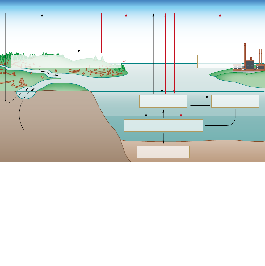
2.1 > The carbon cycle in the 1990s with the sizes of the various
reservoirs (in gigatons of carbon, Gt C), as well as the annual
fluxes between these. Pre-industrial natural fluxes are shown
in black, anthropogenic changes in red. The loss of 140 Gt C
in the terrestrial biosphere reflects the cumulative CO
2
emis-
sions from land-use change (primarily slash and burn agricul-
ture in the tropical rainforests), and is added to the 244 Gt C
emitted by the burning of fossil fuels. The terrestrial sink for
anthropogenic CO
2
of 101 Gt C is not directly verifiable, but
is derived from the difference between cumulative emissions
(244 + 140 = 384 Gt C) and the combination of atmospheric
increase (165 Gt C) and oceanic sinks (100 + 18 = 118 Gt C).
Rivers 0.8
Weathering
0.2
Weathering
0.2
Surface ocean
900 + 18
Intermediate and deep ocean
37 100 + 100
Surface sediment
150
0.2
50
7070.6
0.4
39
11
22.220
6.4
Marine biota
3
Fossil fuels
3700 – 244
Atmosphere
597 + 165
Reservoir sizes in Gt C
Fluxes and rates in Gt C per year
90.2
1.6
101
Land
sink
2.6
Land
use
change
1.6
Respiration
119.6
GPP
120
Vegetation, soil and detritus
2300 + 101 – 140

> Chapter 02
30
Iron is a crucial nutrient for plants and the second most abundant
chemical element on Earth, although the greatest portion by far is
locked in the Earth’s core. Many regions have sufficient iron for
plants. In large regions of the ocean, however, iron is so scarce that
the growth of single-celled algae is limited by its absence. Iron-
limitation regions include the tropical eastern Pacific and parts of
the North Pacific, as well as the entire Southern Ocean. These ocean
regions are rich in the primary nutrients (macronutrients) nitrate and
phosphate. The iron, however, which plants require only in very
small amounts (micronutrients), is missing. Scientists refer to these
marine regions as HNLC regions (high nutrient, low chlorophyll)
because algal growth here is restricted and the amount of the plant
pigment chlorophyll is reduced accordingly. Research using fertiliza-
tion experiments has shown that plant growth in all of these regions
can be stimulated by fertilizing the water with iron. Because plants
assimilate carbon, carbon dioxide from the atmosphere is thus con-
verted to biomass, at least for the short term.
Iron fertilization is a completely natural phenomenon. For exam-
ple, iron-rich dust from deserts is blown to the sea by the wind. Iron
also enters the oceans with the meltwater of icebergs or by contact
of the water with iron-rich sediments on the sea floor. It is presumed
that different wind patterns and a dryer atmosphere during the last
ice age led to a significantly higher input of iron into the Southern
Ocean. This could, at least in part, explain the considerably lower
atmospheric CO
2
levels during the last ice age. Accordingly, modern
modelling simulations indicate that large-scale iron fertilization of
the oceans could decrease the present atmospheric CO
2
levels by
around 30 ppm (parts per million). By comparison, human activities
have increased the atmospheric CO
2
levels from around 280 ppm to
a present-day value of 390 ppm.
Marine algae assimilate between a thousand and a million times
less iron than carbon. Thus even very low quantities of iron are
sufficient to stimulate the uptake of large amounts of carbon dioxide
in plants. Under favourable conditions large amounts of CO
2
can be
converted with relatively little iron. This raises the obvious idea of
fertilizing the oceans on a large scale and reducing the CO
2
concen-
trations in the atmosphere by storage in marine organisms (seques-
tration). When the algae die, however, and sink to the bottom and
are digested by animals or broken down by microorganisms, the car-
bon dioxide is released again. In order to evaluate whether the fixed
Fertilizing the ocean with iron
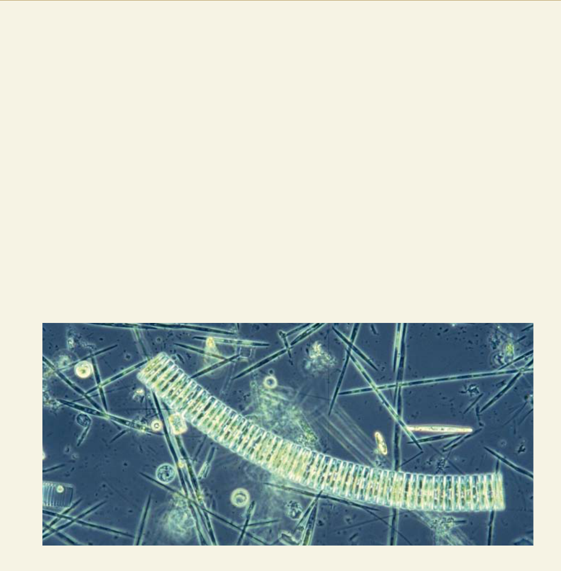
2.2 > Iron is a crucial nutrient for algae, and it is scarce in many ocean
regions, which inhibits algal growth. If the water is fertilized with iron
there is a rapid increase in algae. Microscopic investigations of water
samples taken by the research vessel “Polarstern” clearly show that
algae in this iron-poor region proliferate quickly after iron fertilization.
Around three weeks after fertilization the marine algal community was
dominated by elongate, hard-shelled diatoms.
31
How climate change alters ocean chemistry <
carbon dioxide actually remains in the ocean, the depth at which the
biomass produced by iron fertilization is broken down and carbon
dioxide is released must be known, because this determines its
spatial and temporal distance from the atmosphere. Normally, 60 to
90 per cent of the biomass gets broken down in the surface water,
which is in contact with the atmosphere. So this portion of the bio-
mass does not represent a contribution to sequestration. Even if the
breakdown occurs at great depths, the CO
2
will be released into the
atmosphere within a few hundred to thousand years because of the
global ocean circulation.
There are other reasons why iron fertilization is so controversial.
Some scientists are concerned that iron input will disturb the nutrient
budget in other regions. Because the macronutrients in the surface
water are consumed by increased algal growth, it is possible that
nutrient supply to other downstream ocean regions will be deficient.
Algal production in those areas would decrease, counteracting the
CO
2
sequestration in the fertilized areas. Such an effect would be
expected, for example, in the tropical Pacific, but not in the South-
ern Ocean where the surface water, as a rule, only remains at the sea
surface for a relatively short time, and quickly sinks again before the
macronutrients are depleted. Because these water masses then
remain below the surface for hundreds of years, the Southern Ocean
appears to be the most suitable for CO
2
sequestration. Scientists are
concerned that iron fertilization could have undesirable side effects.
It is possible that iron fertilization could contribute to local ocean
acidification due to the increased decay of organic material and thus
greater carbon dioxide input into the deeper water layers. Further-
more, the decay of additional biomass created by fertilization would
consume more oxygen, which is required by fish and other animals.
The direct effects of reduced oxygen levels on organisms in the rela-
tively well-oxygenated Southern Ocean would presumably be very
minor. But the possibility that reduced oxygen levels could have
long-range effects and exacerbate the situation in the existing low-
oxygen zones in other areas of the world ocean cannot be ruled out.
The possible consequences of iron fertilization on species diversity
and the marine food chain have not yet been studied over time
frames beyond the few weeks of the iron fertilization experiments.
Before iron fertilization can be established as a possible procedure
for CO
2
sequestration, a clear plan for observing and recording the
possible side effects must first be formulated.
> Chapter 02
32
human-made atmospheric CO
2
, and this special property
of seawater is primarily attributable to carbonation,
which, at 10 per cent, represents a significant proportion
of the dissolved inorganic carbon in the ocean. In the
ocean, the carbon dissolved in the form of CO
2
, bicarbo -
nate and carbonate is referred to as inorganic carbon.
When a new carbon equilibrium between the atmos-
phere and the world ocean is re-established in the future,
then the oceanic reservoir will have assimilated around
80 per cent of the anthropogenic CO
2
from the atmos-
phere, primarily due to the reaction with carbonate. The
buffering effect of deep-sea calcium carbonate sediments
is also important. These ancient carbonates neutralize
large amounts of CO
2
by reacting with it, and dissolving
to some extent. Thanks to these processes, the oceans
could ultimately absorb around 95 per cent of the anthro-
pogenic emissions. Because of the slow mixing of the
ocean, however, it would take centuries before equilib-
rium is established. The very gradual buffering of CO
2
by
the reaction with carbonate sediments might even take
millennia. For today’s situation this means that a marked
carbon disequilibrium between the ocean and atmos-
phere will continue to exist for the decades and centuries
to come. The world ocean cannot absorb the greenhouse
gas as rapidly as it is emitted into the atmosphere by
humans. The absorptive capacity of the oceans through
chemical processes in the water is directly dependent
on the rate of mixing in the world ocean. The current
oceanic uptake of CO
2
thus lags significantly behind its
chemical capacity as the present-day CO
2
emissions occur
much faster than they can be processed by the ocean.
Measuring exc h a nge between t h e
atmosphere and ocean
For dependable climate predictions it is extremely impor-
tant to determine exactly how much CO
2
is absorbed by
the ocean sink. Researchers have therefore developed a
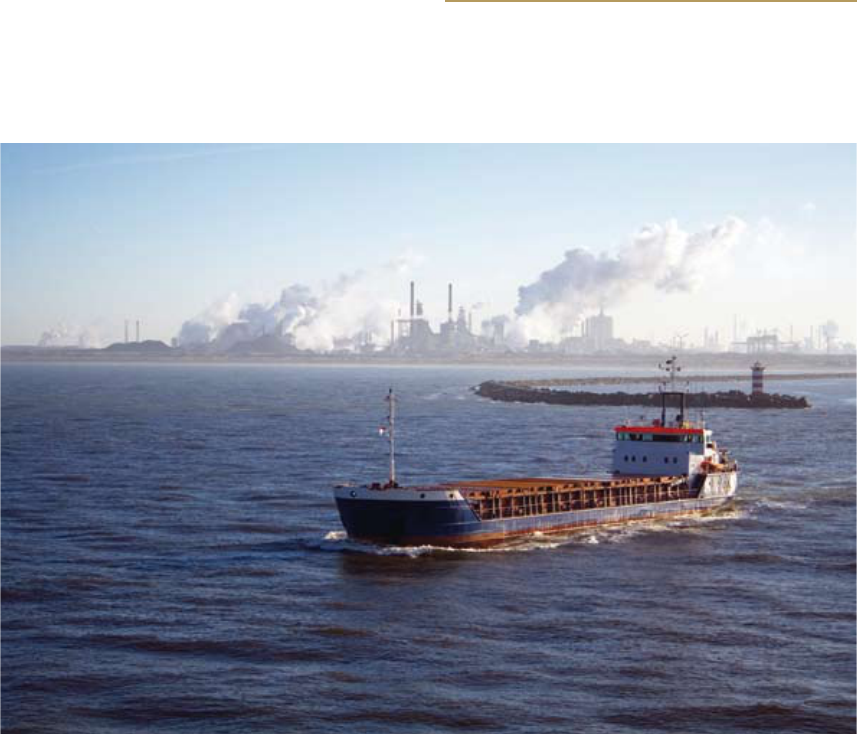
2.3 > Cement plants
like this one in
Amsterdam are,
second to the burning
of fossil fuels, among
the most significant
global sources of
anthropogenic carbon
dioxide. The potential
for reducing CO
2
output is accordingly
large in these
industrial areas.
33
How climate change alters ocean chemistry <
variety of independent methods to quantify the present
role of the ocean in the anthropogenically impacted
carbon cycle. These have greatly contributed to the
present-day understanding of the interrelationships. Two
procedures in particular have played an important role:
The first method (atmosphere-ocean flux) is based on
the measurement of CO
2
partial-pressure differences be-
tween the ocean surface and the atmosphere. Partial
pressure is the amount of pressure that a particular gas
such as CO
2
within a gas mixture (the atmosphere) con-
tributes to the total pressure. Partial pressure is thus also
one possibility for quantitatively describing the composi-
tion of the atmosphere. If more of this gas is present, its
partial pressure is higher. If two bodies, such as the at-
mosphere and the near-surface layers of the ocean, are in
contact with each other, then a gas exchange between
them can occur. In the case of a partial-pressure differ-
ence between the two media, there is a net exchange of
CO
2
. The gas flows from the body with the higher partial
pressure into that of lower pressure. This net gas ex-
change can be calculated when the global distribution of
the CO
2
partial-pressure difference is known. Consider-
ing the size of the world ocean this requires an enormous
measurement effort. The worldwide fleet of research
vessels is not nearly large enough for this task. A signifi-
cant number of merchant vessels were therefore out-
fitted with measurement instruments that automatically
carry out CO
2
measurements and store the data during
their voyages or even transmit them daily via satellite.
This “Voluntary Observing Ship” project (VOS) has been
developed and expanded over the last two decades and
employs dozens of ships worldwide. It is fundamentally
very difficult to adequately record the CO
2
exchange in
the world ocean, because it is constantly changing
through space and time. Thanks to the existing VOS net-
work, however, it has been possible to obtain measure-
ments to provide an initial important basis. The database,
covering over three decades, is sufficient to calculate the
average annual gas exchange over the total surface of the
oceans with some confidence. It is given as average
annual CO
2
flux density (expressed in mol C/m
2
/year),
that is the net flux of CO
2
per square meter of ocean sur-
face per year, which can be integrated to yield the total
annual CO
2
uptake of the world ocean.
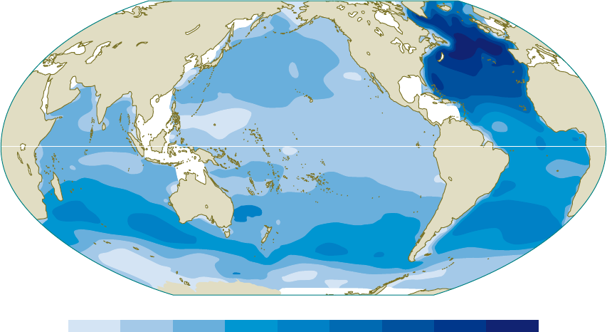
0 10 20 30 40 50 60 70 80
Moles per square metre of water column
Equator
2.4 > The world ocean
takes up anthropo-
genic CO
2
everywhere
across its surface.
The transport into
the interior ocean,
however, primarily
takes place in the
North Atlantic and
in a belt between
30 and 50 degrees
south latitude. The
values indicate the
total uptake from
the beginning of the
industrial revolution
until the year 1994.
> Chapter 02
34
Our present picture is based on around three million
measurements that were collected and calculated for the
CO
2
net flux. The data were recorded between 1970 and
2007, and most of the values from the past decade were
obtained through the VOS programme. Regions that are
important for world climate such as the subpolar North
Atlantic and the subpolar Pacific have been reasonably
well covered. For other ocean regions, on the other hand,
there are still only limited numbers of measurements.
For these undersampled regions, the database is present-
ly insufficient for a precise calculation. Still, scientists
have been able to use the available data to fairly well
quantify the oceanic CO
2
sink. For the reference year
2000 the sink accounts for 1.4 Gt C.
This value represents the net balance of the natural car-
bon flux out of the ocean into the atmosphere and, con-
versely, the transport of anthropogenic carbon from the
atmosphere into the ocean. Now, as before, the annual
natural pre-industrial amount of 0.6 Gt C is flowing out of
the ocean. Conversely, around 2.0 Gt C of anthropo genic
carbon is entering the ocean every year, leading to
the observed balance uptake of 1.4 Gt C per year. Be-
cause of the still rather limited amount of data, this meth-
od has had to be restricted so far to the climato logical CO
2
flux, i.e., a long-term average over the entire observation
period. Only now are studies beginning to approach the
possibility of looking at interannual varia bility for this
CO
2
sink in especially well-covered regions. The North
Atlantic is a first prominent example. Surprisingly, the
data shows significant variations between individual
years. Presumably, this is attributable to natural climate
cycles such as the North Atlantic Oscillation, which have
a considerable impact on the natural carbon cycle. Under-
standing such natural variability of the ocean is a pre-
requisite for reliable projections of future development
and change of the oceanic sink for CO
2
.
The second method attempts, with the application of
rather elaborate geochemical or statistical procedures, to
calculate how much of the CO
2
in the ocean is derived
from natural sources and how much is from anthropo-
genic sources, although from a chemical aspect the two
are basically identical, and cannot be clearly distin-
guished. Actually, several procedures are available today
that allow this difficult differentiation, and they general-
ly provide very consistent results. These methods differ,
however, in detail, depending on the assumptions and
approximations associated with a particular method. The
most profound basis for estimating anthropogenic CO
2
in the ocean is the global hydrographic GLODAP data-
set (Global Ocean Data Analysis Project), which was
obtained from 1990 to 1998 through large international
research projects. This dataset:
• includes quality-controlled data on a suite of carbon
and other relevant parameters;
• is based on analyses of more than 300,000 water
samples;
• containsdatathatwerecollectedonnearly100expe-
ditions and almost 10,000 hydrographic stations in the
ocean.
All of these data were corrected and subjected to multi-
level quality control measures in an elaborate process.
This provided for the greatest possible consistency and
comparability of data from a number of different laborato-
ries. Even today, the GLODAP dataset still provides the
most exact and comprehensive view of the marine carbon
cycle. For the first time, based on this dataset, reliable
estimateshave been made of how much anthropogenic
carbon dioxide has been taken up from the atmosphere
by the ocean sink. From the beginning of industrialization
to the year 1994, the oceanic uptake of anthropogenic car-
bon dioxide amounts to 118 ± 19 Gt C. The results indi-
cate that anthropogenic CO
2
, which is taken up every-
where across the ocean’s surface flows into the ocean’s
interior from the atmosphere primarily in two regions.
One of these is the subpolar North Atlantic, where the
CO
2
submerges with deep-water formation to the ocean
depths. The other area of CO
2
flux into the ocean is a belt
between around 30 and 50 degrees of southern latitude.
Here the surface water sinks because of the formation of
water that spreads to intermediate depths in the ocean.
The CO
2
input derived from the GLODAP dataset to
some extent represents a snapshot of a long-term transi-
tion to a new equilibrium. Although the anthropogenic
carbon dioxide continuously enters the ocean from the
35
How climate change alters ocean chemistry <
surface, the gas has not penetrated the entire ocean by
any means. The GLODAP data show that the world ocean
has so far only absorbed around 40 per cent of the car-
bon dioxide discharged by humans into the atmosphere
between 1800 and 1995. The maximum capacity of the
world ocean of more than 80 per cent is therefore far
from being achieved.
How climate c h a nge impacts t h e
marine carbon cycle
The natural carbon cycle transports many billions of tons
of carbon annually. In a physical sense, the carbon
is spatially transported by ocean currents. Chemically,
it changes from one state to another, for example, from
inorganic to organic chemical compounds or vice versa.
The foundation for this continuous transport and conver-
sion is made up of a great number of biological, chemical
and physical processes that constitute what is also known
as carbon pumps. These processes are driven by climatic
factors, or at least strongly influenced by them. One
example is the metabolism of living organisms, which is
stimulated by rising ambient temperatures. This tempe-
rature effect, however, is presumably less significant for
the biomass producers (mostly single-celled algae) than
for the biomass consumers (primarily the bacteria),
which could cause a shift in the local organic carbon
balance in some regions. Because many climatic inter-
actions are still not well understood, it is difficult to pre-
dict how the carbon cycle and the carbon pumps will
react to climate change. The first trends indicating
change that have been detected throughout the world
ocean are those of water temperature and salinity. In
addition, a general decrease in the oxygen content of
seawater has been observed, which can be attributed to
biological and physical causes such as changes in current
flow and higher temperatures. It is also possible that
changes in the production and breakdown of biomass in
the ocean play a role here.
Changes in the carbon cycle are also becoming
apparent in another way: The increasing accumulation
of carbon dioxide in the sea leads to acidification of the
oceans or, in chemical terms, a decline in the pH value.
This could have a detrimental impact on marine organ-
isms and ecosystems. Carbonate-secreting organisms are
particularly susceptible to this because an acidifying
environment is less favorable for carbonate production.
Laboratory experiments have shown that acidification
has a negative effect on the growth of corals and other
organisms. The topic of ocean acidification is presently
being studied in large research programmes worldwide.
Conclusive results relating to the feedback effects
between climate and acidification are thus not yet avail-
able. This is also the case for the impact of ocean warm-
ing. There are many indications for significant feedback
effects here, but too little solid knowledge to draw any
robust quantitative conclusions.
We will have to carry out focussed scientific studies to
see what impact global change will have on the natural
carbon cycle in the ocean. It would be naïve to assume
that this is insignificant and irrelevant for the future
climate of our planet. To the contrary, our limited knowl-
edge of the relationships should motivate us to study the
ocean even more intensely and to develop new methods
of observation.
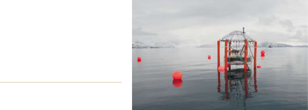
2.5 > In order to determine the effect of increasing atmospheric CO
2
concentrations on
the ocean, an international research team enriched seawater with CO
2
in floating tanks off
Spitsbergen, and studied the effects on organisms.

> Chapter 02
36
How climate change acidifies the oceans
Carbon dioxide is a determining factor for our climate
and, as a greenhouse gas, it contributes considerably to
the warming of the Earth’s atmosphere and thus also of
the ocean. The global climate has changed drastically
many times through the course of Earth history. These
changes, in part, were associated with natural fluctua-
tions in the atmospheric CO
2
content, for example, dur-
ing the transitions from ice ages to interglacial periods
(the warmer phases within longer glacial epochs). The
drastic increase in atmospheric CO
2
concentrations by
more than 30 per cent since the beginning of industriali-
zation, by contrast, is of anthropogenic origin, i.e. caused
by humans.
The largest CO
2
sources are the burning of fossil fuels,
including natural gas, oil, and coal, and changes in land
usage: clearing of forests, draining of swamps, and
expansion of agricultural areas. CO
2
concentrations in
the atmo s phere have now reached levels near 390 ppm
(parts per million). In pre-industrial times this value was
only around 280 ppm. Now climate researchers estimate
that the level will reach twice its present value by the
end of this century. This increase will not only cause
additional warming of the Earth. There is another effect
associated with it that has only recently come to the
atten tion of the public – acidification of the world ocean.
There is a permanent exchange of gas between the air
and the ocean. If the CO
2
levels in the atmosphere
increase, then the concentrations in the near-surface
layers of the ocean increase accordingly. The dissolved
carbon dioxide reacts to some extent to form carbonic
acid. This reaction releases protons, which leads to acidi-
fication of the seawater. The pH values drop. It has been
demonstrated that the pH value of seawater has in fact
already fallen, parallel to the carbon dioxide increase in
the atmosphere, by an average of 0.1 units. Depending
on the future trend of carbon dioxide emissions, this
value could fall by another 0.3 to 0.4 units by the end of
this century. This may appear to be negligible, but in fact
it is equivalent to an increased proton concentration of
100 to 150 per cent.
The effect of pH on the metabol i s m
of marine organisms
The currently observed increase of CO
2
concentrations in
the oceans is, in terms of its magnitude and rate, unparal-
leled in the evolutionary history of the past 20 million
years. It is therefore very uncertain to what extent the
marine fauna can adapt to it over extended time periods.
After all, the low pH values in seawater have an adverse
effect on the formation of carbonate minerals, which is
critical for many invertebrate marine animals with carbo-
nate skeletons, such as mussels, corals or sea urchins.
Processes similar to the dissolution of CO
2
in seawater
also occur within the organic tissue of the affected organ-
isms. CO
2
, as a gas, diffuses through cell membranes into
the blood, or in some animals into the hemolymph, which
is analogous to blood. The organism has to compensate
for this disturbance of its natural acid-base balance, and
some animals are better at this than others. Ultimately
this ability depends on the genetically determined effi-
ciency of various mechanisms of pH and ion regulation,
The consequences of ocean acidification
> C lim at e c h a nge n ot o n ly l e ad s to w a r m ing o f t h e at m o sp he r e an d wa t e r,
but also to an acidification of the oceans. It is not yet clear what the ultimate consequences of this
will be fo r m ar in e o rg a n is ms a n d c om mu nit ie s , a s onl y a fe w s pe c ie s h a v e b e e n st u die d . E x t en sive
long-term studies on a large variety of organisms and communities are needed to understand poten-
tial consequences of ocean acidification.
The pH value
The pH value is a
measure of the
strength of acids and
bases in a solution.
It indicates how acidic
or basic a liquid is.
The pH scale ranges
from 0 (very acidic)
to 14 (very basic).
The stronger an acid
is the more easily it
loses protons (H
+
),
which determines the
pH value. Practically
expressed, the higher
the proton concen-
tration is, the more
acidic a liquid is, and
the lower its pH value
is.
37
How climate change alters ocean chemistry <
which depends on the animal group and lifestyle. In spite
of enhanced regulatory efforts by the organism to regu-
late them, acid-base parameters undergo permanent
adjustment within tissues and body fluids. This, in turn,
can have an adverse effect on the growth rate or repro-
ductive capacity and, in the worst case, can even threat-
en the survival of a species in its habitat.
The pH value of body fluids affects biochemical reac-
tions within an organism. All living organisms therefore
strive to maintain pH fluctuations within a tolerable
range. In order to compensate for an increase in acidity
due to CO
2
, an organism has two possibilities: It must
either increase its expulsion of excessive protons or take
up additional buffering substances, such as bicarbonate
ions, which bind protons. For the necessary ion regula-
tion processes, most marine animals employ specially
developed epithelia that line body cavities, blood vessels,
or the gills and intestine.
The ion transport systems used to regulate acid-base
balance are not equally effective in all marine animal
groups. Marine organisms are apparently highly tolerant
of CO
2
when they can accumulate large amounts of bi-
carbonate ions, which stabilize the pH value. These orga-
nisms are usually also able to very effectively excrete
protons. Mobile and active species such as fish, certain
crustaceans, and cephalopods – cuttlefish, for instance –
are therefore especially CO
2
-tolerant. The metabolic
rates of these animals can strongly fluctuate and reach
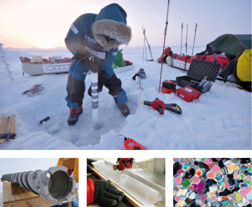
2.6 > By studying ice
cores scientists want
to discover which
organisms live in the
ice. Air bubbles in
Antarctic ice cores
also provide clues to
the presence of trace
gases in the former
atmosphere, and to
past climate. The ice
cores are drilled using
powerful tools. For
more detailed study
they are analysed in
the laboratory.
When ice crystals
are observed under
a special polarized
light, their fine
structure reveals
shimmering colours.

> Chapter 02
38
The atmospheric gas carbon dioxide (CO
2
) dissolves very easily in
water. This is well known in mineral water, which often has carbon
dioxide added. In the dissolution process, carbon dioxide reacts with
the water molecules according to the equation below. When carbon
dioxide mixes with the water it is partially converted into carbonic
acid, hydrogen ions (H
+
), bicarbonate (HCO
3
–
), and carbonate ions
(CO
3
2–
). Seawater can assimilate much more CO
2
than fresh water.
The reason for this is that bicarbonate and carbonate ions have been
perpetually discharged into the sea over aeons. The carbonate reacts
with CO
2
to form bicarbonate, which leads to a further uptake of
CO
2
and a decline of the CO
3
2–
concentration in the ocean. All of
the CO
2
-derived chemical species in the water together, i.e. carbon
dioxide, carbonic acid, bicarbonate and carbonate ions, are referred
to as dissolved inorganic carbon (DIC). This carbonic acid-carbonate
equilibrium determines the amount of free protons in the seawater
and thus the pH value.
CO
2
+ H
2
O
H
2
CO
3
H
+
+ HCO
3
–
2 H
+
+ CO
3
2–
In summary, the reaction of carbon dioxide in seawater proceeds
as follows: First the carbon dioxide reacts with water to form car-
bonic acid. This then reacts with carbonate ions and forms bicarbo-
nate. Over the long term, ocean acidification leads to a decrease in
the concentration of carbonate ions in seawater. A 50 per cent decline
When carbonate formation loses equilibrium
2.7 > Studies of the coral Oculina patagonia show that organisms with
carbonate shells react sensitively to acidification of the water. Picture
a shows a coral colony in its normal state. The animals live retracted
within their carbonate exoskeleton (yellowish). In acidic water (b) the
carbonate skeleton degenerates. The animals take on an elongated polyp
form. Their small tentacles, which they use to grab nutrient particles
in the water, are clearly visible. Only when the animals are transferred
to water with natural pH values do they start to build their protective
skeletons again (c).
a b
c
39
How climate change alters ocean chemistry <
of the levels is predicted, for example, if there is a drop in pH levels
of 0.4 units. This would be fatal. Because carbonate ions together
with calcium ions (als CaCO
3
) form the basic building blocks of car-
bonate skeletons and shells, this decline would have a direct effect
on the ability of many marine organisms to produce biogenic carbo-
nate. In extreme cases this can even lead to the dissolution of exist-
ing carbonate shells, skeletons and other structures.
Many marine organisms have already been studied to find out
how acidification affects carbonate formation. The best-known exam-
ples are the warm-water corals, whose skeletons are particularly
threatened by the drop in pH values. Scientific studies suggest that
carbon dioxide levels could be reached by the middle of this century
at which a net growth (i.e. the organisms form more carbonate than
is dissolved in the water), and thus the successful formation of reefs,
will hardly be possible. In other invertebrates species, such as mus-
sels, sea urchins and starfish, a decrease in calcification rates due to
CO
2
has also been observed. For many of these invertebrates not
only carbonate production, but also the growth rate of the animal
was affected. In contrast, for more active animal groups such as fish,
salmon, and the cephalopod mollusc Sepia officinalis, no evidence
could be found as to know that the carbon dioxide content in the
seawater had an impact on growth rates. In order to draw accurate
conclusions about how the carbon dioxide increase in the water
affects marine organisms, further studies are therefore necessary.
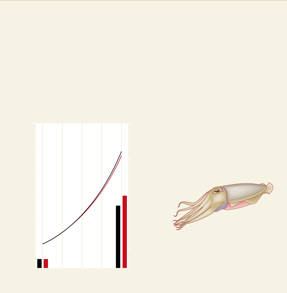
0
5
10
15
20
25
30
Duration of experiment in days
Body weig ht in grams
Amount of c al cium c ar bo nate in c ut tlebone in gra ms
0 10 20 30 40
0
0.6
0.4
0.2
0.8
1.0
1.2
1.4
1.6
2.8 > Active and rapidly moving animals like the cephalopod mollusc
(cuttlefish) Sepia officinalis are apparently less affected by acidification
of the water. The total weight of young animals increased over a period
of 40 days in acidic seawater (red line) just as robustly as in water
with a normal pH and CO
2
content (black line). The growth rate of the
calcareous shield, the cuttlebone, also proceeded at very high rates (see
the red and black bars in the diagram). The amount of calcium carbon-
ate (CaCO
3
) incorporated in the cuttlebone is used as a measure here.
The schematic illustration of the cephalopod shows the position of the
cuttlebone on the animal.
Cuttlebone

> Chapter 02
40
very high levels during exercise (hunting & escape beha-
viour). The oxygen-consumption rate (a measure of meta-
bolic rate) of these active animal groups can reach levels
that are orders of magnitude above those of sea urchins,
starfish or mussels. Because large amounts of CO
2
and
protons accumulate during excessive muscle activity, ac-
tive animals often possess an efficient system for proton
excretion and acid-base regulation. Consequently, these
animals can better compensate for disruptions in their
acid-base budgets caused by acidification of the water.
Benthic invertebrates (bottom-dwelling animals with-
out a vertebral column) with limited ability to move great
distances, such as mussels, starfish or sea urchins, often
cannot accumulate large amounts of bicarbonate in their
body fluids to compensate for acidification and the excess
protons. Long-term experiments show that some of these
species grow more slowly under acidic conditions. One
reason for the reduced growth could be a natural protec-
tive mechanism of invertebrate animal species: In stress
situations such as falling dry during low tide, these
organisms reduce their metabolic rates. Under normal
conditions this is a very effective protection strategy
that insures survival during short-term stress situations.
But when they are exposed to long-term CO
2
stress,
this protective mechanism could become a disadvantage
for the sessile animals. With the long-term increase in
carbon dioxide levels in seawater, the energy-saving
behaviour and the suppression of metabolism inevitably
leads to limited growth, lower levels of activity, and thus
a reduced ability to compete within the ecosystem.
However, the sensitivity of a species’ reaction to CO
2
stressor and acidification cannot be defined alone by the
simple formula: good acid-base regulation = high CO
2
tolerance. There are scientific studies that suggest this is
not the case. For example, one study investigated the
ability of a species of brittlestar (echinodermata), an
invertebrate that mainly lives in the sediment, to regen-
erate severed arms. Surprisingly, animals from more
acidic seawater not only re-grew longer arms, but their
calcareous skeletons also contained a greater amount of
calcium carbonate. The price for this, however, was
reduced muscle growth. So in spite of the apparent posi-
tive indications at first glance, this species is obviously
adversely affected by ocean acidification because they
2.9 > Diatoms like
this Arachnoidiscus
are an important
nutrient basis for
higher organisms.
It is still uncertain
how severely they
will be affected by
acidification of the
oceans.
41
How climate change alters ocean chemistry <
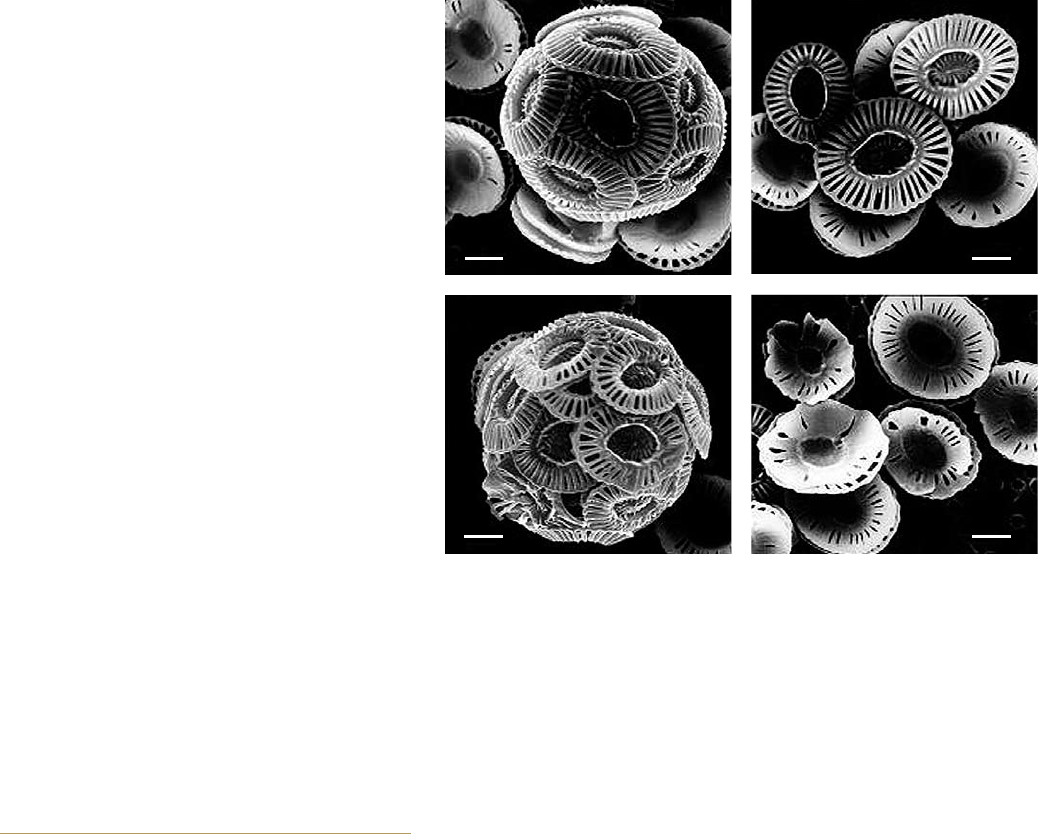
2.10 > These electron micrographs clearly illustrate that increased CO
2
concentrations in
the water can disturb and lead to malformation in calcareous marine organisms, such as
the coccolithophorid Emiliana huxleyi shown here. The upper pictures reflect CO
2
concen-
trations in the water of 300 ppm, which is slightly above the pre-industrial average CO
2
level for seawater. The bottom photographs reflect a CO
2
content of 780 to 850 ppm. For
size comparison, the bars represent a length of one micrometre.
can only efficiently feed and supply their burrows in the
sediment with oxygenated seawater if they have fully
functioning arms.
Even fish can be impaired. Many adult animals are
relatively CO
2
tolerant. Early developmental stages, how-
ever, obviously react very sensitively to the CO
2
stressor.
A strong impairment of the sense of smell in seawater
with low pH values was observed in the larval clown-
fish. These animals are normally able to orientate them-
selves by a specific odour signal and, after their larval
phase, which they spend free-swimming in the water
column, to find their final permanent habitat on coral
reefs. In the experiment, fish larvae that were raised in
seawater with a pH value lowered by about 0.3 units,
reacted significantly less to the otherwise very stimulat-
ing odour of sea anemones with which they live in sym-
biosis on reefs. If behavioural changes caused by CO
2
occur during a critical phase of the life cycle, they can, of
course, have a strong impact on the reproductive success
of a species.
It is not yet known to what extent other marine orga-
nisms are impacted by these kinds of effects of ocean
acidification. Other studies on embryonic and juvenile
stages of various species have shown, however, that the
early developmental stages of an organism generally
respond more sensitively to CO
2
stress than the adult
animals do.
Threat to the n utrition bas e in the ocean s –
phytoplankton and acidification
The the entire food chain in the ocean is represented by
the microscopic organisms of the marine phytoplankton.
These include diatoms (siliceous algae), coccolithophores
(calcareous algae), and the cyanobacteria (formerly called
blue algae), which, because of their photosynthetic
activity, are responsible for around half of the global
primary productivity.
Because phytoplankton requires light for these pro-
cesses, it lives exclusively in surface ocean waters. It is
therefore directly affected by ocean acidification. In the
future, however, due to global warming, other influenc-
ing variables such as temperature, light or nutrient avail-
ability will also change due to global warming. These
changes will also determine the productivity of auto-
trophic organisms, primarily bacteria or algae, which
produce biomass purely by photosynthesis or the incor-
poration of chemical compounds. It is therefore very dif-
ficult to predict which groups of organisms will profit
from the changing environmental conditions and which
will turn out to be the losers.
Ocean acidification is of course not the only conse-
quence of increased CO
2
. This gas is, above all, the elixir
of life for plants, which take up CO
2
from the air or
seawater and produce biomass. Except for the acidifica-
tion problem, increasing CO
2
levels in seawater should

> Chapter 02
42
2.11 > The clownfish (Amphiprion
percula) normally does not react
sensitively to increased CO
2
concen-
trations in the water. But in the
larvae the sense of smell is impaired.

43
How climate change alters ocean chemistry <
therefore favour the growth of those species whose
photosynthetic processes were formerly limited by car-
bon dioxide. For example, a strong increase in photo-
synthesis rates was reported for cyanobacteria under
higher CO
2
concentrations. This is also true for certain
coccolithophores such as Emiliania huxleyi. But even for
Emiliania the initially beneficial rising CO
2
levels could
become fatal. Emiliania species possess a calcareous
shell comprised of numerous individual plates. There is
now evidence that the formation of these plates is
impaired by lower pH values. In contrast, shell formation
by diatoms, as well as their photosynthetic activity,
seems to be hardly affected by carbon dioxide. For
diatoms also, however, shifts in species composition
have been reported under conditions of increased CO
2
concentration.
Challenge for the future:
Understanding acidification
In order to develop a comprehensive understanding of
the impacts of ocean acidification on life in the sea, we
have to learn how and why CO
2
affects various physio-
logical processes in marine organisms. The ultimate
critical challenge is how the combination of individual
processes determines the overall CO
2
tolerance of the
organisms. So far, investigations have mostly been limit-
ed to short-term studies. To find out how and whether an
organism can grow, remain active and reproduce success-
fully in a more acidified ocean, long term (months) and
multiple-generation studies are neccessary.
The final, and most difficult step, thus is to integrate
the knowledge gained from species or groups at the eco-
system level. Because of the diverse interactions among
species within ecosystems, it is infinitely more difficult
to predict the behaviour of such a complex system under
ocean acidification.
In addition, investigations are increasingly being
focused on marine habitats that are naturally charac-
terized by higher CO
2
concentrations in the seawater.
Close to the Italian coast around the island of Ischia, for
instance, CO
2
is released from the sea floor due to vol-
canic activity, leading to acidification of the water. This
means that there are coastal areas directly adjacent to
one another with normal (8.1 to 8.2) and significantly
lowered pH values (minimum 7.4). If we compare the
animal and plant communities of these respective areas,
clear differences can be observed: In the acidic areas
rock corals are completely absent, the number of speci-
mens of various sea urchin and snail species is low, as is
the number of calcareous red algae. These acidic areas of
the sea are mainly dominated by seagrass meadows and
various non-calcareous algal species.
The further development of such ecosystem-based
studies is a great challenge for the future. Such investi-
gations are prerequisite to a broader understanding of
future trends in the ocean. In addition, deep-sea eco-
systems, which could be directly affected by the possible
impacts of future CO
2
disposal under the sea floor, also
have to be considered.
In addition, answers have to be found to the question
of how climate change affects reproduction in various
organisms in the marine environment. Up to now there
have been only a few exemplary studies carried out and
current science is still far from a complete understanding.
Whether and how different species react to chemical
changes in the ocean, whether they suffer from stress
or not is, for the most part, still unknown. There is an
enormous need for further research in this area.
2.12 > Low pH values in the waters around Ischia cause corrosion of the shells of calcare-
ous animals such as the snail Osilinus turbinata. The left picture shows an intact spotted
shell at normal pH values of 8.2. The shell on the right, exposed to pH values of 7.3, shows
clear signs of corrosion. The scale bars are equal to one centimetre.

> Chapter 02
44
Oxygen – product and elixir of life
Carbon dioxide, which occurs in relatively small amounts
in the atmosphere, is both a crucial substance for plants,
and a climate-threatening gas. Oxygen, on the other
hand, is not only a major component of the atmosphere,
it is also the most abundant chemical element on Earth.
The emergence of oxygen in the atmosphere is the result
of a biological success model, photosynthesis, which
helps plants and bacteria to convert inorganic materials
such as carbon dioxide and water to biomass. Oxygen
was, and continues to be generated by this process. The
biomass produced is, for its part, the nutritional founda-
tion for consumers, either bacteria, animals or humans.
These consumers cannot draw their required energy
from sunlight as the plants do, rather they have to obtain
it by burning biomass, a process that consumes oxygen.
Atmospheric oxygen on our planet is thus a product, as
well as the elixir of life.
Oxygen budget for the world ocean
Just like on the land, there are also photosynthetically
active plants and bacteria in the ocean, the primary pro-
ducers. Annually, they generate about the same amount
of oxygen and fix as much carbon as all the land plants
together. This is quite amazing. After all, the total living
biomass in the ocean is only about one two-hundredth of
that in the land plants. This means that primary pro-
ducers in the ocean are around two hundred times more
productive than land plants with respect to their mass.
This reflects the high productivity of single-celled algae,
which contain very little inactive biomass such as, for
example, the heartwood in tree trunks. Photosynthetic
production of oxygen is limited, however, to the upper-
most, sunlit layer of the ocean. This only extends to a
depth of around 100 metres and, because of the stable
density layering of the ocean, it is largely separated from
the enormous underlying volume of the deeper ocean.
Moreover, most of the oxygen generated by the primary
producers escapes into the atmosphere within a short
time, and thus does not contribute to oxygen enrichment
in the deep water column. This is because the near-sur-
face water, which extends down to around 100 metres,
is typically saturated with oxygen by the supply from the
atmosphere, and thus cannot store additional oxygen
from biological production. In the inner ocean, on the
Oxygen in the ocean
> Scientis t s have been routi n e ly measur i n g oxygen concentrati o n s in th e
ocean for more than a hundred years. With growing concerns about climate change, however, this
parameter has suddenly become a hot topic. Dissolved oxy g e n in the ocea n provides a s e n sitive
early warning system for the tren d s t h a t c l imate change is causing. A massiv e de p l oyment of oxygen
sensors is projected for the coming years, which will represent a renaissance of this parameter.
2.13 > Marine animals react in different ways to oxygen
deficiency. Many species of snails, for instance, can tolerate
lower O
2
levels than fish or crabs. The diagram shows the con-
centration at which half of the animals die under experimental
conditions. The average value is shown as a red line for each
animal group. The bars show the full spectrum: some crusta-
ceans can tolerate much lower O
2
concentrations than others.
0 50 100 150 200 250
Snails
Mussels
Fishes
Crustaceans
Average lethal
oxygen concentration
in micromoles per litre
45
How climate change alters ocean chemistry <
other hand, there is no source of oxygen. Oxygen enters
the ocean in the surface water through contact with the
atmosphere. From there the oxygen is then brought to
greater depths through the sinking and circulation of
water masses. These, in turn, are dynamic processes that
are strongly affected by climatic conditions. Three factors
ultimately determine how high the concentration of dis-
solved oxygen is at any given point within the ocean:
1. The initial oxygen concentration that this water pos-
sessed at its last contact with the atmosphere.
2. The amount of time that has passed since the last
contact with the atmosphere. This can, in fact, be
decades or centuries.
3. Biological oxygen consumption that results during this
time due to the respiration of all the consumers. These
range from miniscule bacteria to the zooplankton, and
up to the higher organisms such as fish.
The present-day distribution of oxygen in the internal
deep ocean is thus determined by a complicated and not
fully understood interplay of water circulation and bio-
logical productivity, which leads to oxygen consumption
in the ocean’s interior. Extensive measurements have
shown that the highest oxygen concentrations are found
at high latitudes, where the ocean is cold, especially
well-mixed and ventilated. The mid-latitudes, by con-
trast, especially on the western coasts of the continents,
are characterized by marked oxygen-deficient zones. The
oxygen supply here is very weak due to the sluggish
water circulation, and this is further compounded by
elevated oxygen consumption due to high biological pro-
ductivity. This leads to a situation where the oxygen is
almost completely depleted in the depth range between
100 and 1000 metres. This situation is also observed in
the northern Indian Ocean in the area of the Arabian Sea
and the Bay of Bengal.
Different groups of marine organisms react to the
oxygen deficiency in completely different ways, because
of the wide range of tolerance levels of different marine
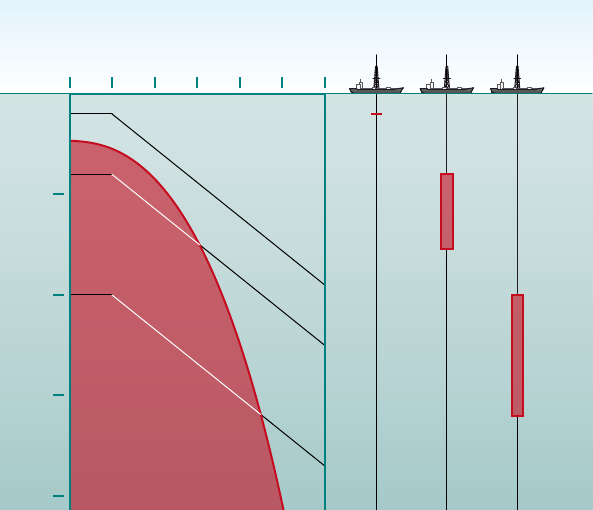
Sur face layer
pyncnocline
at ca. 100 m
Sea floor
Sea level
Atmosphere
ca. 4000 m
ca. 1000 m
Inter me diate waterDee p water
Antarctic Equator Arctic
Oxygen decrease due to biological processes
Oxygen decrease
due to biological processes
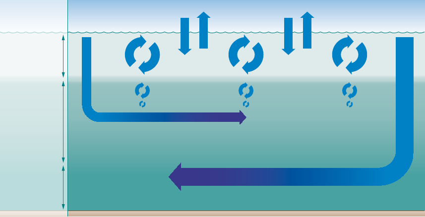
2.14 > Oxygen from the atmosphere enters the near-surface
waters of the ocean. This upper layer is well mixed, and is thus
in chemical equilibrium with the atmosphere and rich in O
2
.
It ends abruptly at the pyncnocline, which acts like a barrier.
The oxygen-rich water in the surface zone does not mix readily
with deeper water layers. Oxygen essentially only enters the
deeper ocean by the motion of water currents, especially with
the formation of deep and intermediate waters in the polar
regions. In the inner ocean, marine organisms consume oxygen.
This creates a very sensitive equilibrium.
> Chapter 02
46
expected decrease in oxygen transport from the atmos-
phere into the ocean that is driven by global current and
mixing processes, as well as possible changes in the
marine biotic communities. In recent years, this knowl-
edge has led to a renaissance of oxygen in the field of
global marine research.
In oceanography, dissolved oxygen has been an impor-
tant measurement parameter for over a hundred years. A
method for determining dissolved oxygen was developed
as early as the end of the 19th century, and it is still
applied in an only slightly modified form today as a
precise method. This allowed for the development of an
early fundamental understanding of the oxygen distribu-
tion in the world ocean, with the help of the famous Ger-
man Atlantic Expedition of the “Meteor” in the 1920s.
Research efforts in recent years have recorded decreas-
ing oxygen concentrations for almost all the ocean basins.
These trends are, in part, fairly weak and mainly limited
to water masses in the upper 2000 metres of the ocean.
animals to oxygen-poor conditions. For instance, crusta-
ceans and fish generally require higher oxygen concen-
trations than mussels or snails. The largest oceanic oxy-
gen minimum zones, however, because of their ex tremely
low concentrations, should be viewed primarily as natu-
ral dead zones for the higher organisms, and by no means
as caused by humans.
Oxygen – the renaissance of a
hydrographic parameter
Oxygen distribution in the ocean depends on both bio-
logical processes, like the respiration of organisms, and
on physical processes such as current flow. Changes in
either of these processes should therefore lead to changes
in the oxygen distribution. In fact, dissolved oxygen can
be viewed as a kind of sensitive early warning system for
global (climate) change in the ocean. Scientific studies
show that this early warning system can detect the
5
5
10
10
10
25
25
50
50
50
75
75
75
100
100
100
Equator
0°
125
125
125
150
200
150
150
Oxygen conce ntr ation at the ox yge n m inimum
in m icromo les p er lit re
0
10
50
100
200
150
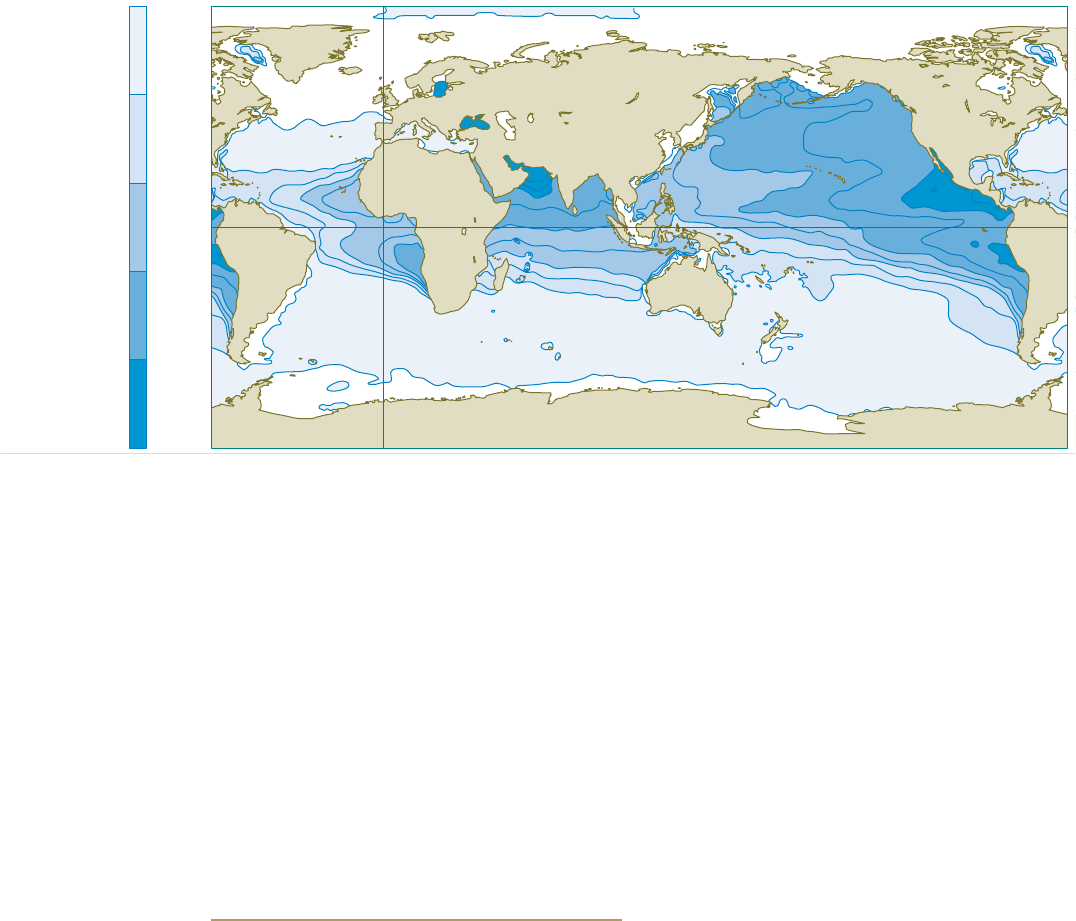
2.15 > Marine regions with oxygen deficiencies are completely
natural. These zones are mainly located in the mid-latitudes
on the west sides of the continents. There is very little mixing
here of the warm surface waters with the cold deep waters,
so not much oxygen penetrates to greater depths. In addition,
high bioproductivity and the resulting large amounts of sin-
king biomass here lead to strong oxygen consumption at depth,
especially between 100 and 1000 metres.

47
How climate change alters ocean chemistry <
Therefore, no fully consistent picture can yet be drawn
from the individual studies. Most of the studies do, how-
ever, show a trend of decreasing oxygen concentrations.
This trend agrees well with an already verified expan-
sion and intensification of the natural oxygen minimum
zones, those areas that are deadly for higher organisms.
If the oxygen falls below certain (low) thres hold values,
the water becomes unsuitable for higher organisms. Ses-
sile, attached organisms die. Furthermore, the oxygen
deficiency leads to major changes in biogeochemical
reactions and elemental cycles in the ocean – for instance,
of the plant nutrients nitrate and phosphate.
Oxygen levels affect geochemical processes in the
sediment but also, above all, bacterial metabolism pro-
cesses, which, under altered oxygen conditions, can be
changed dramatically. It is not fully possible today to pre-
dict what consequences these changes will ultimately
have. In some cases it is not even possible to say with
certainty whether climate change will cause continued
warming, or perhaps even local cooling. But it is prob-
able that the resulting noticeable effects will continue
over a long time period of hundreds or thousands of
years.
Even today, however, climate change is starting to
cause alterations in the oxygen content of the ocean that
can have negative effects. For the first time in recent
years, an extreme low-oxygen situation developed off the
coast of Oregon in the United States that led to mass mor-
tality in crabs and fish. This new death zone off Oregon
originated in the open ocean and presumably can be
attributed to changes in climate. The prevailing winds off
the west coast of the USA apparently changed direction
and intensity and, as a result, probably altered the ocean
currents. Researchers believe that the change caused
oxygen-poor water from greater depths to flow to surface
waters above the shelf.
The death zone off Oregon is therefore different than
the more than 400 near-coastal death zones known
worldwide, which are mainly attributed to eutrophica-
tion, the excessive input of plant nutrients. Eutrophi-
cation normally occurs in coastal waters near densely
populated regions with intensive agricultural activity.
Oxygen – challenge to marine research
The fact that model calculations examining the effects of
climate change almost all predict an oxygen decline in
major parts of the ocean, which agrees with the available
observations of decreasing oxygen, gives the subject
additional weight. Even though the final verdict is not yet
in, there are already indications that the gradual loss of
oxygen in the world ocean is an issue of great relevance
which possibly also has socio-economic repercussions,
and which ocean research must urgently address.
Intensified research can provide more robust conclu-
sions about the magnitude of the oxygen decrease. In
addition it will contribute significantly to a better under-
standing of the effects of global climate change on the
ocean. In recent years marine research has addressed
this topic with increased vigour, and has already estab-
lished appropriate research programmes and projects. It
is difficult, however, to completely measure the tempo-
rally and spatially highly variable oceans in their totality.
In order to draw reliable conclusions, therefore, the clas-
sic instruments of marine research like ships and taking
water samples will not suffice. Researchers must begin
to apply new observational concepts.
“Deep drifters” are an especially promising tool: these
are submersible measuring robots that drift completely
autonomously in the ocean for 3 to 4 years, and typically
measure the upper 2000 metres of the water column
every 10 days. After surfacing, the data are transferred to
a data centre by satellite. There are presently around
3200 of these measuring robots deployed for the interna-
tional research programme ARGO, named after a ship
from Greek mytho logy. Together they form a world-
wide autonomous ob ser vatory that is operated by almost
30 countries.
So far this observatory is only used on a small scale for
oxygen measurements. But there has been developed a
new sensor technology for oxygen measurements in the
recent past that can be deployed on these drifters. This
new technology would give fresh impetus to the collec-
tion of data on the variability of the oceanic oxygen
distribu tion.
The Atlantic
Expedition
For the first time,
during the German
Atlantic Expedition
(1925 to 1927)
with the research
vessel “Meteor”,
an entire ocean
was systematically
sampled, both in the
atmosphere and in
the water column.
Using an echosounder
system that was
highly modern for
its time, depth profiles
were taken across
13 transits of the
entire ocean basin.
> Chapter 02
48
How methane ends up in the ocean
People have been burning coal, oil and natural gas for
more than a hundred years. Methane hydrates, on the
other hand, have only recently come under controversial
discussion as a potential future energy source from the
ocean. They represent a new and completely untapped
reservoir of fossil fuel, because they contain, as their
name suggests, immense amounts of methane, which is
the main component of natural gas. Methane hydrates
belong to a group of substances called clathrates – sub-
stances in which one molecule type forms a crystal-like
cage structure and encloses another type of molecule. If
the cage-forming molecule is water, it is called a hydrate.
If the molecule trapped in the water cage is a gas, it is a
gas hydrate, in this case methane hydrate.
Methane hydrates can only form under very specific
physical, chemical and geological conditions. High water
pressures and low temperatures provide the best condi-
tions for methane hydrate formation. If the water is
warm, however, the water pressure must be very high
in order to press the water molecule into a clathrate cage.
In this case, the hydrate only forms at great depths. If the
water is very cold, the methane hydrates could conceiv-
ably form in shallower water depths, or even at atmos-
pheric pressure. In the open ocean, where the average
bottom-water temperatures are around 2 to 4 degrees
Celsius, methane hydrates occur starting at depths of
around 500 metres.
Surprisingly, there is no methane hydrate in the
deepest ocean regions, the areas with the highest pres-
sures, because there is very little methane available here.
The reason for this is because methane in the ocean is
produced by microbes within the sea floor that break
down organic matter that sinks down from the sunlit
zone near the surface.
Organic matter is co mposed, for example, of the re -
mains of dead algae and animals, as well as their excre-
ments. In the deepest areas of the ocean, below around
2000 to 3000 metres, only a very small amount of
organic remains reach the bottom because most of them
are broken down by other organisms on their way down
through the water column. As a rule of thumb, it can be
said that only around 1 per cent of the organic material
produced at the surface actually ends up in the deep sea.
The deeper the sea floor is, the less organic matter settles
on the bottom. Methane hydrates therefore primarily
occur on the continental slopes, those areas where the
Climate change impacts on methane hydrates
> Huge amounts of me t h ane are stored a r ound the world i n the sea floor i n
the form of solid methane hydrates. These hydrates represent a large energy reserve for humanity.
Climate warming, however, could cause the hydrates to destabilize. The methane, a potent green-
house gas, would escape unused into the atmosphere and could even accelerate climate change.
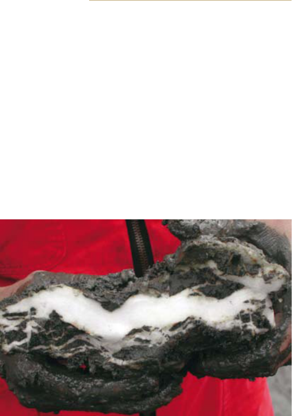
2.16 > Methane
hydrate looks like a
piece of ice when it is
brought up from the
sea floor. This lump
was retrieved during
an expedition to the
“hydrate ridge” off
the coast of Oregon
in the US.
49
How climate change alters ocean chemistry <
continental plates meet the deep-sea regions. Here there
is sufficient organic matter accumulating on the bottom
and the combination of temperature and pressure is
favourable. In very cold regions like the Arctic, methane
hydrates even occur on the shallow continental shelf
(less than 200 metres of water depth) or on the land in
permafrost, the deep-frozen Arctic soil that does not
even thaw in the summer.
It is estimated that there could be more potential fossil
fuel contained in the methane hydrates than in the
classic coal, oil and natural gas reserves. Depending on
the mathematical model employed, present calculations
of their abundance range between 100 and 530,000 giga-
tons of carbon. Values between 1000 and 5000 gigatons
are most likely. That is around 100 to 500 times as much
carbon as is released into the atmosphere annually by
the burning of coal, oil and gas. Their possible future
excavation would presumably only produce a portion of
this as actual usable fuel, because many deposits are
inaccessible, or the production would be too expensive
or require too much effort. Even so, India, Japan, Korea
and other countries are presently engaged in the devel-
opment of mining techniques in order to be able to use
methane hydrates as a source of energy in the future
(Chapter 7).
Methane hydrates and global warming
Considering that methane hydrates only form under very
specific conditions, it is conceivable that global warming,
which as a matter of fact includes warming of the oceans,
could affect the stability of gas hydrates.
There are indications in the history of the Earth sug-
gesting that climatic changes in the past could have led
to the destabilization of methane hydrates and thus to
the release of methane. These indications – including
measurements of the methane content in ice cores, for
instance – are still controversial. Yet be this as it may, the
issue is highly topical and is of particular interest to
scientists concerned with predicting the possible impacts
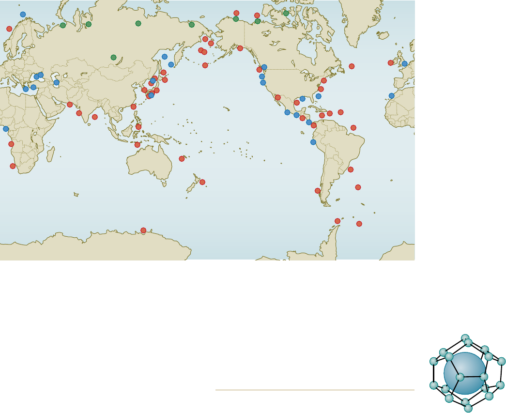
2.17 > Methane
hydrate occurs in
all of the oceans as
well as on land. The
green dots show
occurrences in the
northern permafrost
regions. Occurrences
identified by geo-
physical methods are
indicated by red. The
occurrences shown
by blue dots were
verified by direct
sampling.
2.18 > In hydrates,
the gas (large ball)
is enclosed in a cage
formed by water
molecules. Scientists
call this kind of
molecular arrange-
ment a clathrate.
> Chapter 02
50
of a temperature increase on the present deposits of
methane hydrate.
Methane is a potent greenhouse gas, around 20 times
more effective per molecule than carbon dioxide. An
increased release from the ocean into the atmosphere
could further intensify the greenhouse effect. Investiga-
tions of methane hydrates stability in dependance of tem-
perature fluctuations, as well as of methane behaviour
after it is released, are therefore urgently needed.
Various methods are employed to predict the future
development. These include, in particular, mathematic
modelling. Computer models first calculate the hypo-
thetical amount of methane hydrates in the sea floor
using background data (organic content, pressure, tem-
perature). Then the computer simulates the warming of
the seawater, for instance, by 3 or 5 degrees Celsius per
100 years. In this way it is possible to determine how the
methane hydrate will behave in different regions. Calcu-
lations of methane hydrate deposits can than be coupled
with complex mathematical climate and ocean models.
With these computer models we get a broad idea of how
strongly the methane hydrates would break down under
the various scenarios of temperature increase. Today it is
assumed that in the worst case, with a steady warming
of the ocean of 3 degrees Celsius, around 85 per cent of
the methane trapped in the sea floor could be released
into the water column.
Other, more sensitive models predict that methane
hydrates at great water depths are not threatened by
warming. According to these models, only the methane
hydrates that are located directly at the boundaries of the
stability zones would be primarily affected. At these
locations, a temperature increase of only 1 degree Celsius
would be sufficient to release large amounts of methane
from the hydrates. The methane hydrates in the open
ocean at around 500 metres of water depth, and deposits
in the shallow regions of the Arctic would mainly be
affected.
In the course of the Earth’s warming, it is also expected
that sea level will rise due to melting of the polar ice caps
and glacial ice. This inevitably results in greater pressure
at the sea floor. The increase in pressure, however, would
not be sufficient to counteract the effect of increasing
temperature to dissolve the methane hydrates. Accor-
ding to the latest calculations, a sea-level rise of ten
metres could slow down the methane-hydrate dissoluti-
on caused by a warming of one degree Celsius only by a
few decades.
A wide variety of mathematical models are used to
predict the consequences of global warming. The results
of the simulations are likewise very variable. It is there-
fore difficult to precisely evaluate the consequences of
global warming for the gas hydrate deposits, not least of
all because of the large differences in the calculations of
the size of the present-day gas hydrate deposits. One
major goal of the current gas hydrate research is to
optimize these models by using ever more precise input
parameters. In order to achieve this, further measure-
ments, expeditions, drilling and analyses are essential.
Drill hole in
400 m
water depths
100 m 1000 m
Zone of
ga s hydrate
s t ab ility
Zone of
ga s hydrate
s t ab ility
100 m
400 m
770 m
1000 m
1600 m
Temperature in degrees Celsius
–5 5 10 15 20 250
Dept h
in metre s
500
1000
1500
2000
Gas hydrates = unstable
Gas hydrates = stable
2.19 > Gas hydrates occur when sufficient methane is produced by organic matter degrada-
tion in the sea floor under low temperature and high pressure conditions. These conditions
occur predominantly on the continental margins. The warmer the water, the larger the water
depths must be to form the hydrate. Deep inside he sea floor, however, the temperature is
too high for the formation of methane hydrates because of the Earth’s internal heat.
Oxidation
Many bacteria use
methane to provide
energy for their meta-
bolism. They take up
methane and trans-
form it chemically.
In this process the
methane releases
electrons and is thus
oxidized. Some bacte-
ria break the methane
down with the help of
oxygen. This is called
aerobic oxidation.
Other bacteria do not
need oxygen. This
kind of oxidation is
called anaerobic.
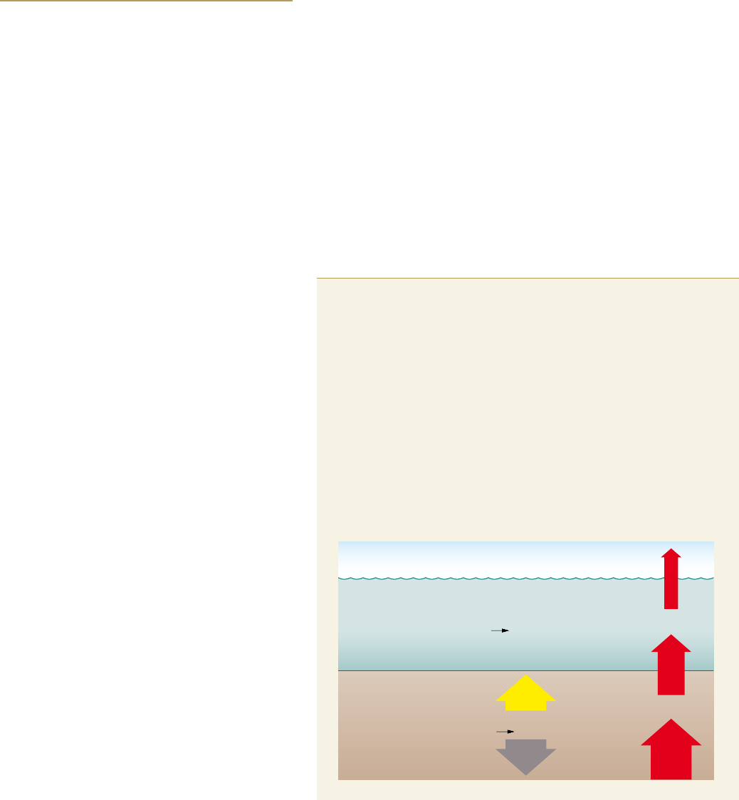
51
How climate change alters ocean chemistry <
What happens when methane hydrate melts?
Not all the methane that is released from unstable
methane hydrates ends up in the atmosphere. The great-
est portion is likely to be broken down during its rise
through the sediments and in the water column. This
decomposition is mediated by two biological processes:
• anaerobic oxidation of methane by bacteria and
archaea (formerly called archaebacteria) within the
sea floor;
• aerobicoxidationofmethanebybacteriainthewater
column.
During anaerobic oxidation of methane in the sediment
the microbes use sulphate (SO
4
2–
), the salt of sulphuric
acid that is present in large quantities in sea water, for
the methane decomposition. In this process methane is
converted to bicarbonate (HCO
3
–
). If the bicarbonate
reacts further with calcium ions (Ca
2+
) in the seawater,
calcium carbonate (CaCO
3
) precipitates, which remains
stored in the sea floor over long periods of time. That
would be the ideal situation, because it would make the
potent greenhouse gas methane (CH
4
) harmless. At the
same time, hydrogen sulphide (H
2
S) is produced from
the sulphate, which provides energy to chemosynthetic
communities, including symbiotic clams and tube-
worms. During aerobic oxidation in the water column,
however, bacteria break down methane with the help of
oxygen (O
2
). In this process, carbon dioxide is produced,
which dissolves in the water. Carbon dioxide contributes
to ocean acidification. Furthermore, aerobic oxidation of
methane consumes oxygen. The depletion of oxygen in
the water column could create or expand oxygen mini-
mum zones in the ocean, which are a threat for fishes
and other sensitive organisms. Rough estimates suggest
that anaerobic and aerobic oxidation of methane together
currently convert around 90 per cent of the methane pro-
duced in the sea floor before it can reach the atmosphere.
The more slowly methane migrates through the sea floor
or through the water column, the more effective the
microbes are in converting it.
A prerequisite for this kind of degradation is that the
methane molecules are dissolved in water. Methane can
only be degraded by the bacteria in this form. If the
methane is released rapidly from the hydrates, it could
rise in the form of gas bubbles that are not accessible by
microorganisms. The microbial methane filter would
thus fail, at least in part, if the methane hydrates break
down very rapidly and large quantities of methane are
released at once.
There is also a problem at shallow water depths, where
the methane bubbles cannot completely dissolve in the
water over the short distance from the sea floor to the
atmosphere. In order to better understand such processes
and to be able to make predictions about the functions of
the microbial filters, researchers are currently investi-
gating natural methane sources on the sea floor, so-called
Bacteria convert methane
Methane (CH
4
) in the ocean is to a large extend consumed by microorgan-
isms. During anaerobic decay within the sea floor, microbes convert methane
with the help of sulphate (SO
4
2–
). This process produces hydrogen sulphide
anions (HS
–
) and hydrogen sulphide (H
2
S), which are closely related chemi-
cally and occur naturally together, as well as bicarbonate (CaCO
3
). Bicarbo-
nate can react with calcium ions (Ca
2+
) to precipitate as calcium carbonate
(CaCO
3
). During aerobic decay (in the water column) oxygen (O
2
) from the
water is consumed. Carbon dioxide (CO
2
) and water (H
2
O) are produced. If
large amounts of methane are released in the future from the gas hydrates
in the sea floor, aerobic decay could result in the creation of oxygen mini-
mum zones. The carbon dioxide produced could also contribute to ocean
acidification.
Atmosphere
Water column
Sea floor
Anaerobic methane oxidation
HCO
3
–
+ HS
–
+ H
2
OCH
4
+ SO
4
2
–
Aerobic methane oxidation
CO
2
+ 2H
2
OCH
4
+ 2O
2
CH
4
CaCO
3
H
2
S
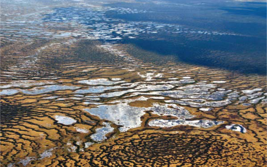
> Chapter 02
52
cold seeps, which constantly release larger quantities of
methane. These include near-surface gas hydrate depo-
sits, mud volcanoes, and natural-gas seeps in shallow
marine regions. These seeps are a kind of natural model
where the behaviour of methane in the ocean can be
studied. If we understand how nature reacts to these
methane seeps at the sea floor, it will help us to estimate
the consequences of larger methane releases from gas
hydrates. The data obtained at the methane seeps should
also help to improve the precision of mathematical
methane hydrate simulations.
The disappearance of methane hydrates could have
fatal consequences. Gas hydrates act like a cement that
fills the pores between the fine sediment particles and
stabilizes the sea floor. If the methane hydrates decom-
pose, the stability of the sea floor is reduced due to the
missing cement and the possible generation of excess
pore pressure. In the worst case, large parts of continen-
tal margins fail. The resulting submarine landslides might
cause severe tsunamis.
Massive mass movements occurred during the last ice
age and the following deglaciation. The trigger was prob-
ably not always warming of the atmosphere, but also the
opposite. Because large quantities of water were stored
in the ice during the last ice age, sea level was around
120 metres lower than it is today. Especially in the shal-
low ocean regions, the water pressure was so low that
massive amounts of methane hydrate could have been
destabilized. Direct evidences for such slope failures
caused by decomposing gas hydrates have not yet been
found. There are, however, some indications suggesting
a process in the past. Signs of seeping fluids are almost
2.20 > Large quantities of methane hydrate are stored not only
in the sea floor, but also on land, especially in the perpetually
frozen permafrost ground of the Russian tundra, such as here
in the Russian republic of Komi. Scientists are concerned that
the permafrost soils could melt due to global warming and
thus release the methane hydrates.

53
How climate change alters ocean chemistry <
Conclusion
Material fluxes – getting the full picture
The chemical and geochemical processes in the
ocean are complex. Explaining them in their entire-
ty will be a challenge for decades. There is clear
evidence of global changes, such as the decrease in
oxygen levels and acidification in the oceans. So far,
however, our knowledge is not sufficient to say
with certainty or in detail what impact climate
change will have and how it will affect various
parameters in the future.
It is certain that disturbances caused by climate
change can have very serious consequences,
because the chemical and geochemical material
fluxes amount to many billions of tons. The amount
of methane hydrate bound up in the sea floor alone
is gigantic. If it is released and the methane rises
into the atmosphere, it will have a significant impact
on the development of future climate. Investiga tions
of the chemical and geochemical processes are
therefore of enormous importance if we want to
learn what to expect and how humanity can respond
to it.
Analyses of the CO
2
cycle reveal how the CO
2
reservoirs of the atmosphere, land biomass and
ocean interact. The oceans are buffering increas-
ing concentrations of atmospheric trace gases. But
these processes and reaching a new CO
2
equilibri-
um will take millennia. Natural processes therefore
cannot keep up with the speed at which humans
continue to discharge CO
2
and other climate-rele-
vant trace gases into the air. The only solution is to
save energy and significantly reduce greenhouse
gas emissions.
always found in the vicinity of slope failures. These
slopes were possibly destabilized by gases released by
decomposing gas hydrates and liquids. Researchers also,
however, definitely see the possibility of a reverse rela-
tionship: it is conceivable that slope failures and the
resulting reduction in pressure on underlying sediments
caused the dissociation of methane hydrates at the conti-
nental margins, thereby releasing large amounts of free
gas. The slumps would have been the cause rather than
the result of gas escape. These uncertainties highlight
the need for further research. It is, however, fairly cer-
tain that the disappearance of methane hydrates could
lead to serious problems.
Methane emissions from the Arctic – a prime
focus of future gas hydrate research
In the field of methane emission research today, the
Arctic is one of the most important regions worldwide. It
is believed that methane occurs there both in the form of
gas hydrate in the sea and as free gas trapped in the
deep-frozen permafrost. Methane deposits in permafrost
and hydrates are considered to be very sensitive in the
expansive shallow-shelf regions, because with the rela-
tively low pressures it would only take a small tempera-
ture change to release large amounts of methane. In addi-
tion, new methane is continuously being produced
because the Arctic regions are rich in organic material
that is decomposed by microbes in the sediment. The
activity of these microbes and thus the biological release
rates of methane are also stimulated by increases in tem-
perature. Hence methane emissions in the Arctic have
multiple sources. International scientific consortia are
now being established involving researchers from vari-
ous disciplines – chemists, biologists, geologists, geophy-
sicists, meteorologists – which are intensively addres-
sing this problem. No one can yet say with certainty how
the methane release in the Arctic will develop with glo-
bal warming, either in the ocean or on the land. This
research is still in its in fancy.

pp. 26–27: Steve Gschmeissner/Science Photo Library/Agentur Focus,
Fig. 2.1: after IPCC (2007), Fig. 2.2: dpa Picture-Alliance/DB Philipp Assmy/
Awi, Fig. 2.3: Stephan Köhler/Zoonar, Fig. 2.4: after Sabine et al. (2004),
Fig. 2.5: Nicolai, IFM-GEOMAR, Fig. 2.6: top: Martin Hartley/eyevine/
interTOPICS; left: mauritius images; mid: Carmen Jaspersen/picture- alliance/
dpa; right: Cliff Leight/Aurora Photos, Fig. 2.7: Fine und Tchernov (2007); Foto:
Avinoam Briestien, Fig. 2.8: after Gutowska et al. (2008), Fig. 2.9: Steve
Gschmeissner/Science Photo Library/Agentur Focus, Fig. 2.10: Reprinted by
permission from Macmillan Publishers Ltd: Nature Publishing Group,
U. Riebesell et al., Nature 407, 2000, Fig. 2.11: Mike Watson Images Limited/
Getty Images, Fig. 2.12: Hall-Spencer et al. (2008), Fig. 2.13: after Vaquer-Sunyer
und Duarte (2008), Fig. 2.14: maribus, Fig. 2.15: after Keeling et al. (2010),
Fig. 2.16: dpa Picture-Alliance/MARUM, Fig. 2.17: after Kvenvolden und
Lorenson (1993), Fig. 2.18: maribus, Fig. 2.19: after IFM-GEOMAR, Fig. p. 51:
after Treude, IFM-GEOMAR, Fig. 2.20: imago/ITAR-TASS
Reproduction, translation, microfilming, electronic processing and transmission
in any form or by any means are prohibited without the prior permission in
writing of maribus gGmbH. All the graphics in the World Ocean Review were
produced exclusively by Walther-Maria Scheid, Berlin. The list of illustrations
states the original sources which were used as a basis for the preparation of the
illustrations in some cases.
Table of figures chapter 2
Project manager: Jan Lehmköster
Editing: Tim Schröder
Copy editing: Dimitri Ladischensky
Editorial team at the Cluster of Excellence: Dr. Kirsten Schäfer,
Dr. Emanuel Söding, Dr. Martina Zeller
Design and typesetting: Simone Hoschack
Photo-editing: Petra Kossmann
Graphics: Walther-Maria Scheid
Printing: Druckhaus Berlin-Mitte GmbH
Paper: Recysatin, FSC-certified
ISBN 978-3-86648-012-4
Published by: maribus gGmbH, Pickhuben 2, 20457 Hamburg
www.maribus.com
Publication details
