Contrast Detection Probability - Implementation and use cases
Uwe Artmann, Image Engineering GmbH & Co KG; Kerpen, Germany
Marc Geese, Robert Bosch GmbH, Leonberg, Germany
Max G
¨
ade, Image Engineering GmbH & Co KG; Kerpen, Germany
Abstract
The automotive industry formed the initiative IEEE-P2020
to jointly work on key performance indicators (KPIs) that can be
used to predict how well a camera system suits the use cases. A
very fundamental application of cameras is to detect object con-
trasts for object recognition or stereo vision object matching. The
most important KPI the group is working on is the contrast detec-
tion probability (CDP), a metric that describes the performance
of components and systems and is independent from any assump-
tions about the camera model or other properties. While the the-
ory behind CDP is already well established, we present actual
measurement results and the implementation for camera tests. We
also show how CDP can be used to improve low light sensitivity
and dynamic range measurements.
Introduction
The idea of Contrast Detection Probability (CDP) was first
presented by Geese et.al.[1] in 2018. It was derived from the need
to have a KPI that is independent from the system under test and
also independent from which components are tested. So the same
KPI shall be applied to describe the performance of a windshield
or a lens.
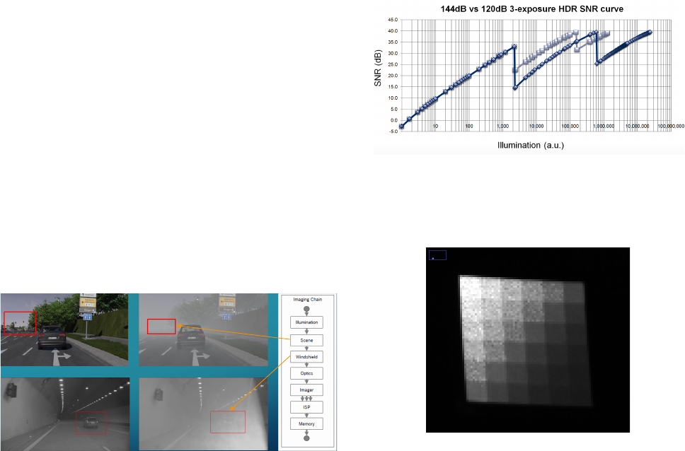
As shown in the examples in Figure 1, the cause for loss
of contrast can be manifold and is not only related to the cam-
era system itself. CDP was designed to describe the performance
of a camera system to reproduce contrasts, the core functionality
needed for advanced algorithms in machine vision.
EXAMPLES FOR LOW OBJECT CONTRAST
Contrast reduction on the input – fog in the scene or dust on the windshield
Figure 1. Different aspects in imaging that can lead to a contrast loss on
the input side of a camera. In these examples this is fog or pollen dust on a
windshield.
Another important new aspect in automotive imaging is High
Dynamic Range and the impact on system performance. As de-
scribed in the IEEE-P2020 white paper [2] and shown in Figure 2,
the HDR rendering process can lead to so called SNR drops. This
is an effect from combining e.g. the dark part of one image with
the bright part of another. The resulting SNR curve will show
drops somewhere between the maximum and minimum light in-
tensity. An example is shown in figure 3. The SNR drop can be
observed in the SNR curve, a plot of the SNR vs. the light in-
tensity. The open question is, how much impact does this have
on the system performance. Even though the SNR value is a well
established metric, it is very hard to derive precise system perfor-
mance predictions from the SNR value. The CDP value has this
possibility, as it is directly related to the system performance.
12
Copyright © 2018 IEEE. All rights reserved.
HDR—High dynamic range imagers are often combined with local tone mapping image processing. This
creates challenges of texture and local contrast preservation, color fidelity/stability, SNR stability (see
Figure 8
), and motion artefacts.
Multi-cam
—In applications such as SVS, image capture originating from multiple cameras with
overlapping field of views are combined or “stitched” together. The created virtual image evaluation is
problematic due to the individual characteristics of each camera and captured portion of the scene, i.e.,
different field
s of view, local processing, different and mixed camera illumination.
Distributed—Distributed systems with some local image
processing close to the imager and some ECU
centralized processing. Local processing (e.g., tone mapping)
does not preserve the original information at
the camera and is
therefore not invertible to be post recovered in the central ECU (e.g., glossy
compression/quantization).
Dual purpose
—The same camera feed may have to serve both for viewing and computer vision needs.
Extrinsic components—System level image quality is affected by additional components of the vehicle
(lights, windshield, protection cover window, etc.).
Video
—Automotive systems use video imagery. Many of current imaging standards, however, were
originally targeted for still image application and typically do not cover motion video image quality.
Illumination—The huge variety of the scene illumination in automotive use cases imposes additional
challenges for testing (e.g., xenon light, d65 light, sunlight, various LED street lamps).
Another issue is that the existing standards do not necessarily cover the
specific challenges that occur in
uncontrolled use environments, in which automotive camera applications need to operate.
Figure 8
shows a typical SNR versus illumination curve of camera using a multi-exposure type of HDR operation.
When
a high dynamic range scene (e.g., tunnel entrance/exit) is captured, a counterintuitive phenomenon may
occur
in regions of the image above the intermediate SNR drop point. Brighter regions above those drops will
exhibit higher noise than regions with a lower brightness. This means that there is more noise in the intermediate
bright regions than in the dark ones. In the case where an application requires a certain minimum level of SNR,
these intermediate drops become an issue because existing standards on HDR do not consider such intermediate
SNR drops. Figure 8
illustrates an example SNR curve of a sensor operated in an optimized configuration to achieve
improved SNR at these drop points. This consequently leads to reduced dynamic range from 144 dB down to
120
dB, according to operation adjustment required to achieve an improved overall SNR level.
Figure 8 SNR vs. illumination for multi exposure HDR imagers
Figure 2. A typical SNR curve for HDR rendering. Depending on different
sensor settings, more or less significant SNR drops occur. Source: IEEE-
P2020
Figure 3. An example image (detail) of the effects also known as SNR drop.
The noise is more dominant in the bright parts of the image compared to the
dark parts. The bright part is rendered from another image than the dark
part.
Concept of Contrast Detection Probability
A single CDP value describes the probability that two sys-
tem outputs (e.g. two digital values) create a contrast from two
system inputs (e.g. two luminance inputs). It is calculated from
two random variables (here A and B). These random variables
IS&T International Symposium on Electronic Imaging 2019
Autonomous Vehicles and Machines Conference 2019 030-1
https://doi.org/10.2352/ISSN.2470-1173.2019.15.AVM-030
© 2019, Society for Imaging Science and Technology
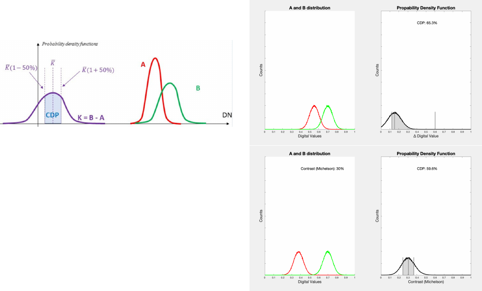
are the distribution of digital values for a flat-field area in an im-
age with a known luminance. A noise free system would have a
distribution where all digital values in a region of interest (ROI)
equals the mean value. A real system will show, depending on
noise and signal processing a distribution of values. From the two
random variables A and B a new random variable K is calculated,
which defines the contrast. K also has a probability density, which
represents the probability to measure or detect a certain contrast.
The CDP value is the area beneath the PDF, limited by a defined
confidence interval.
CDP - MEASUREMENT
• Measures the probability that two digital values (pixels) are different for two different input
luminance values
• Consider the PDFs of the random variables A and B with
̅
" <
$
% for two input luminances
• The CDP is then calculated as the area under the PDF of the difference variable
K within a
defined confidence interval around
$
&
Figure 4. Calculation of CDP based on random variables A and B. The
probability density function K is calculated based on the difference between
A and B. CDP is calculated as the area beneath the PDF limited by a confi-
dence interval of ±50% in this example
The CDP value is not an absolute value, it has parameters
that allow it to be tailored for the demanded use cases. So different
use cases will require different calculation steps and will lead to
different CDP values.
One aspect that needs to be defined is how to calculate the
probability density function K. In our implementation, we choose
a random pairing approach, others might be possible. Random
pairing mean that random pixels from variable A and random pix-
els from variable B are used to calculate K. In case of a simple
difference, the pixel value from a random pixel in A is subtracted
from a random pixel in B. Doing this for all pixels will lead to the
PDF K.
To obtain a stable PDF K, a large amount of random pair-
ings are required. Taking multiple frames of the test scene and
performing the pairing not only between two ROI in one frame,
but also over multiple frames, will increase the total number of
pairings and increase the stability.
Subtracting the pixel values A from B will describe the ab-
solute difference between two patches, the use case would be to
find out if the system under test can generate a difference between
A and B.
Another option is to calculate a contrast value for every com-
bination of pixels in A and B. Different options are e.g. Michelson
contrast or Weber contrast. So every pair of pixels between A and
B will be used to calculate a contrast value, this will generate K.
The use case for this would be to check how well and within which
limitations the system under test will reproduce object contrasts
in an absolute sense. So if a system would increase or decrease
the object contrast, it will lead to a lower CDP value. This can
be required if a system is trained to classify objects based on their
contrast or to find out how much impact an HDR rendering has on
the object contrast.
Another aspect that needs to be derived from the use case and
requirement analysis process is to define the required confidence
interval to calculate CDP. Basically these are the edge cases that
are still acceptable for the use case. A smaller interval will lead
to lower CDP values, making it less likely that the measurement
will fall into the confidence interval.
Examples for different methods to calculate K and the differ-
ences in the confidence interval are shown in figure 5.
Figure 5. Two different scenarios to calculate CDP. top: Calculating the
CDP based on simple difference. The confidence interval is not limited to
the top, higher difference is always accepted bottom: Calculating the CDP
based on Michelson contrast. The confidence interval is limiting too high and
too low contrasts in the image with a confidence interval of ±50%
Each measurement of CDP is a function of many variables,
for example: contrast and luminance. The luminance is the aver-
age of the luminance of A and B and the contrast is the contrast
generated by the luminance of A and B. It is strongly adviced to
measure the CDP for a large amount of combinations of contrast
and luminance. As we have two variables, we can display and
plot the CDP in different ways. A simple and already previously
presented form is the 2D plot as shown in figure 9. Here each plot
line represents a different contrast.
A new approach to present the data is to plot luminance, con-
trast and CDP in the same plot as 3D data, while CDP is either the
height or is represented by a different color encoding. This repre-
sentation was chosen to show measurement data in figure 10.
030-2
IS&T International Symposium on Electronic Imaging 2019
Autonomous Vehicles and Machines Conference 2019
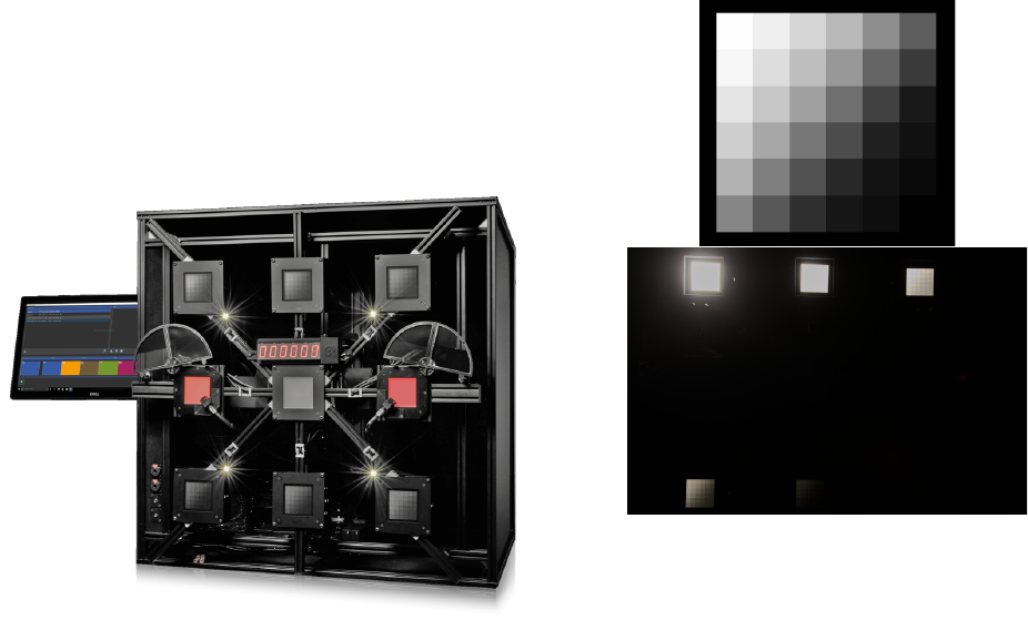
Measurement
We choose a test setup as shown in figure 6. The device un-
der test has to reproduce six test targets, each of them showing 36
gray patches (see Figure 7). Each of the charts is back illuminated
with a dimmable flat field light source. The total contrast that can
be generated is 120dB, each individual chart features a contrast of
10:1.
Figure 6. The measurement device used for this test. The key components
for this test are the six back illuminated test targets, three in the top row, three
in the bottom row. Details of the chart shown in figure 7.
The targets themselves generate 216 measurement points for
one image. Additionally, a dynamic change of the intensity of the
flat field light sources is possible as well and increases the total
amount of measurement points (see Figure 8).
By gathering the image data over time we can increase the
luminance of each light source by 1% for each measurement step
and thus reducing the minimal available contrast steps nominally
to 1%. The target with the highest luminance remains constant
during this procedure to ensure an absolute reference point. There
is a square correlation between the number of available luminance
and the resulting measurement points. A higher number of mea-
surement points increases the probability to find local artifacts in
the measurement.
Several different devices were tested, only very few devices
can be published due to promised confidentially. The results
shown in figure 9 and 10 are obtained from an automotive camera
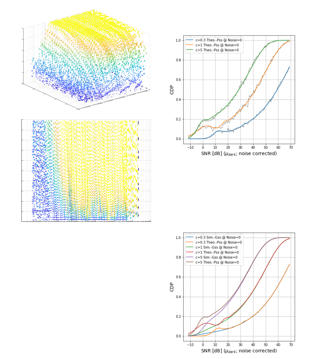
with HDR mode. They show the same data in different represen-
tations.
We can clearly identify so called SNR drops, while we can
now derive information how much this actually affects the poten-
tial contrast detection in the final use case. So we obtain more
useful results than only an SNR curve can do.
Figure 7. Details of the used test system. top: One of the six identical test
targets. Different intensities generated by different back illumination, one
illumination per chart. The combined dynamic range of all charts is 120dB.
bottom: An example image captured by a camera under test.
Linking CDP to SNR
In the annex of this paper we derive a theoretical link be-
tween CDP and SNR by utilizing several assumptions. Please
note again that this calculation of a CDP value from SNR is only
possible if the assumptions for the probability distributions are
valid and if the system under test allows meaningful SNR mea-
surements. Here we present the results of this theoretical deriva-
tion for Poisson-only and Gauss-only systems that are based on
eq. 63 and eq. 44.
Figure 11 shows this derived connection for the noisy Pois-
son system and we can observe that the connection between CDP
and SNR is, as expected, highly nonlinear. To reach a notewor-
thy single measurement detection probability (e.g. CDP > 10%),
an SNR
dB
> 10 is needed. Of course CDP can also be applied to
prefiltered signals, for example to the average of a 3 ×3 neighbor-
hood to improve the detection probabilities.
Figure 12 shows the same connection between CDP and
SNR considering a Gaussian approximation of the probability
densities. The results are similar in the high intensity domain,
however deviate in the low light domain. This shows that for Pois-
son dominant systems a CDP estimation based on a pure Gaussian
noise assumption will lead to significant differences. Especially
for low light use cases such an assumption might lead to a mis-
judgment of the system performance.
To finalize, a comparison of a noisy system is analyzed in
Figure 13. Not depicted are SNR
dB
> 30 and CDP > 0.35 because
CDP and SNR converge to their above already discussed nonlin-
ear connection in this range. In the low light scenarios however,
SNR and CDP seem not to be compatible measures. Even though
the SNR is noise compensated, CDP between 10% −20% yields
to a variety of possible SNR measures e.g. SNR
dB
∈ {0, 5}, de-
IS&T International Symposium on Electronic Imaging 2019
Autonomous Vehicles and Machines Conference 2019 030-3
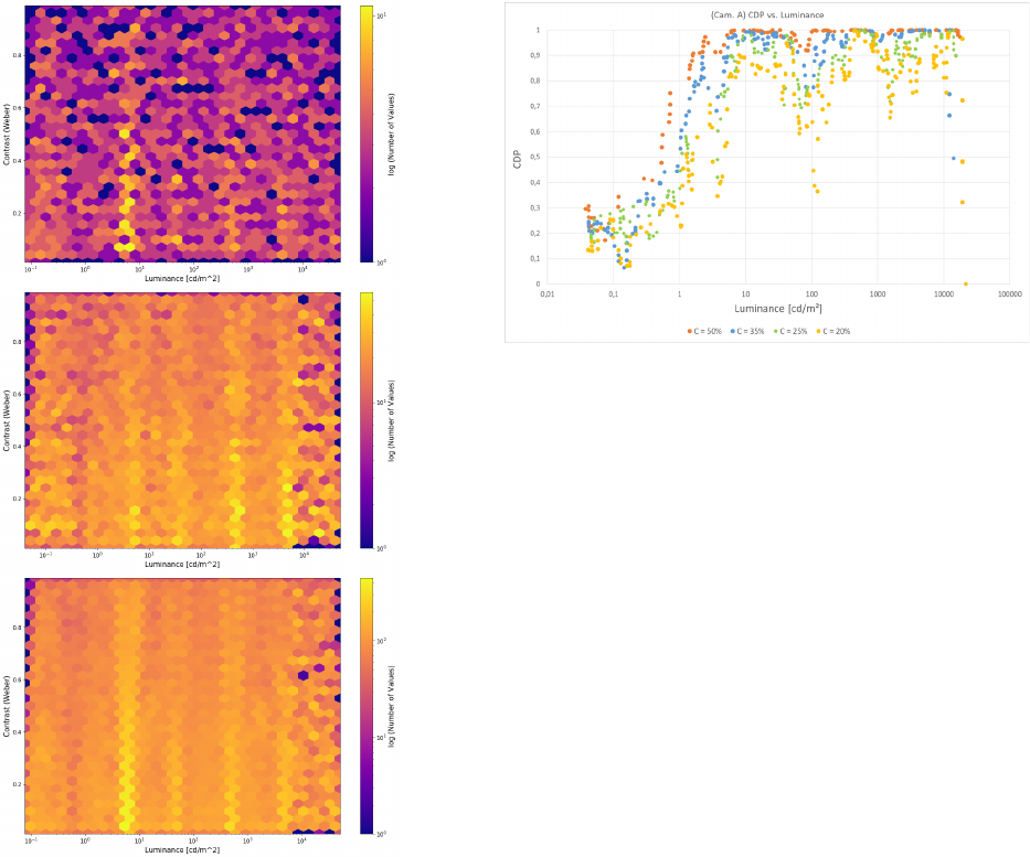
Figure 8. Per luminance and contrast available measurement points as
color code for different measurement modes of the device. The amount of
measurement points will increase by shifting. top: no shifting center: 3 step
shifting bottom: 6 step shifting
pending on the noise in the signal. As typical low light sensitivity
tests are executed in this domain the SNR values seem not to be
able to predict the CDP behavior of the system correctly. The
full shape of the probability density distribution of the connected
noise processes has to be considered to measure the correct CDP
performance.
Future Work
This new representation of 3D CDP visualization from fig.
10 can easily visualize how CDP measurement can also be used
to derive information about dynamic range or sensitivity from a
CDP measurement. Traditionally, these measurements are de-
rived from an SNR measurement, but as the exact meaning of
SNR is questionable, also the usefulness of derived metrics should
be reviewed.
Considering the dynamic range of a system, such a KPI shall
Figure 9. 2D plot of CDP data from an automotive camera with HDR func-
tionality. The different plots represent different contrast level.
describe the range of scene luminance that the system under test
can reproduce. If something is darker or brighter than the mea-
sured maximum and minimum luminance, we have a loss of in-
formation. With new HDR rendering algorithms and the already
explained issues, a pure dynamic range description would exclude
the so called SNR drops. We propose to use CDP to measure dy-
namic range related KPIs.
A dynamic range based on CDP would require to define a
minimum CDP that is accepted and then apply this minimum to
a CDP plot like shown in figure 10. If we set all measurement
points larger than the minimum to 1 and all below the required
minimum to 0, we actually have an area that defines under which
conditions useful data can be obtained from the system.
A typical way to describe sensitivity of a system is the
SNR10 value. This is the luminance that leads to an SNR value
of 10. As we now understand, that the meaning of SNR values is
limited, we should also consider to not use SNR as a metric and
define other measurements.
Conclusion
• The CDP measurement is a new KPI that is directly linked
to the application and use case of the system under test.
• The relation between SNR and CDP is non-linear and de-
pends on noise influences. Only given further assumptions,
CDP be calculated directly from SNR numbers.
• CDP can be used to describe the performance of different
components within the imaging chain using the same metric.
• CDP requires a well defined requirement design. The use
case will define the required calculation of K, the sensitivity
of detection algorithms and the robustness of trained sys-
tems will define the used confidence interval for calculating
CDP.
• When using CDP for standardization, the workgroups need
to provide a framework that makes the reporting of the as-
sumptions made for calculating CDP mandatory and pro-
pose a typical parametrization for CDP.
Acknowledgments
Thanks for the team in the iQ-Lab at Image Engineering
GmbH & Co KG for performing the required tests.
030-4
IS&T International Symposium on Electronic Imaging 2019
Autonomous Vehicles and Machines Conference 2019
0
1
0.2
0.8
0.4
10
4
CDP
0.6
0.6
Contrast
0.8
10
2
Luminance
0.4
1
10
0
0.2
0
10
-2
10
-2
10
-1
10
0
10
1
10
2
10
3
10
4
10
5
Luminance
0
0.1
0.2
0.3
0.4
0.5
0.6
0.7
0.8
0.9
1
Contrast
Figure 10. 3D plot of CDP data from an automotive camera with HDR
functionality. The X and Y axis are luminance and contrast, the Z axis is the
CDP. top: A 3D plot bottom: A 2D plot with CDP represented in the color
coding.
References
[1] Geese, Seger, Paollilo, ”Detection Probabilities: Performance Predic-
tion for Sensors of Autonomous Vehicles”,doi:10.2352/ISSN.2470-
1173.2018.17.AVM-148
[2] IEEE-SA P2020 - Automotive Image Quality Working Group, ”IEEE
White Paper”, ISBN 9781504451130
[3] D. V. Hinkley (December 1969). ”On the Ratio of Two Corre-
lated Normal Random Variables”. Biometrika. 56 (3): 635639.
doi:10.2307/2334671. JSTOR 2334671.
Author Biography
Uwe Artmann studied Photo Technology at the University of Applied
Sciences in Cologne following an apprenticeship as a photographer, and
finished with the German ’Diploma Engineer’. He is now CTO at Image
Engineering, an independent test lab for imaging devices and manufac-
turer of all kinds of test equipment for these devices. His special interest
is the influence of noise reduction on image quality and MTF measurement
in general.
Figure 11. Intensity dependent CDP plots with δ
±
= 0.2 against the mea-
sured SNR values show a nonlinear connection between CDP and SNR.
SNR
dB
> 10 is needed to gain some significant CDP performance for the dis-
cussed use case.
Figure 12. Intensity dependent CDP plots with δ
±
= 0.2 against SNR shows
the nonlinear connection between CDP and SNR and the differences be-
tween the Poisson and Gaussian assumptions when calculating CDP from
SNR values only. Using a Gaussian assumption to calculate CDP from SNR
yields to significant deviation for SNR
dB
< 15.
IS&T International Symposium on Electronic Imaging 2019
Autonomous Vehicles and Machines Conference 2019 030-5
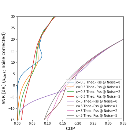
Figure 13. The CDP from SNR connection is also depending on the noise
level of the signal. Only for larger detection probabilities, the CDP to SNR
connection shows independent from noise. In the depicted range a calcula-
tion of the CDP performance is not possible given only the SNR measure-
ments as input.
Marc Geese received a Diploma in applied physics from Frankfurt
University, an MPhil in Electrical Engineering from University of Manch-
ester and a PhD in Physics from Heidelberg University. His research
focused on Complex Systems and Neural Networks applied to Image Pro-
cessing tasks, Vision Chips and Computer Vision Algorithms and special
computer vision algorithms for video based ADAS Systems. In his cur-
rent work is as a system architect for Robert Bosch GmbH his focus is on
the imaging chain consisting of optics, imager and ISP for video based
ADAS systems of the next generation. His special interest is in new KPIs
that serve the automotive image quality standardization and for this he is
leading the subgroup no. 3 of the IEEE P2020 Working group.
Max G
¨
ade is a research and development engineer at Image En-
gineering. After graduating from the University of Applied Sciences in
Cologne with a Bachelor of Engineering degree in Media Technology, his
work now focusses on test solutions for automotive imaging.
030-6
IS&T International Symposium on Electronic Imaging 2019
Autonomous Vehicles and Machines Conference 2019
Annex A
The link between SNR and CDP requires a longer list of assumptions
and calculation steps. As these would make the reading of the paper more
complex, we show them in this annex.
Assumptions to link CDP to component level SNR
All measurement processes and the photon generation itself are
based on random processes which introduce noise into the measurements.
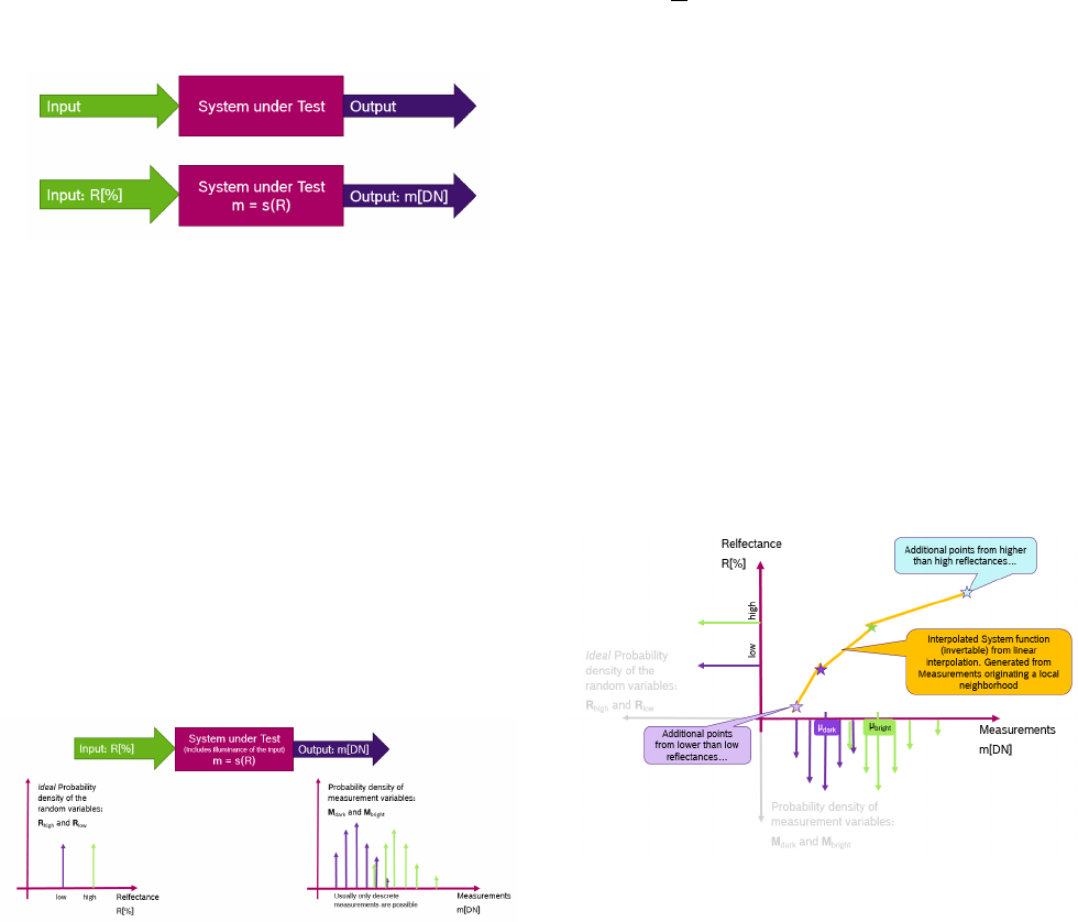
We consider a system under test (SUT), for example a complete
imaging chain or any other applicable subsystem. Figure 14 shows such
a system with two input stimuli R, the system function s and the output
measurement m.
Figure 14. System under test with reflectance input R, and digital output m.
The illuminance conditions are here considered as part of the system.
As described in the CDP definition, two inputs are needed to mea-
sure CDP, which can be generated either by a high and low light emit-
tance, or by a high and low reflectance that is illuminated by a constant
light source. Assuming these input signals as ideal we would observe delta
peaks in their probability density as shown in figure 15.
Measuring the two input reflectances, we obtain a set of bright and
dark measurements (e.g. {m
max,i
}, {m
min,i
}). Of course these measure-
ments depend, among other variables, strongly on the illumination that
has to be considered part of the SUT.
The measurements are not deterministic due to their noise depen-
dencies (e.g. photon flux Poisson noise, dark currents in the image sensors
etc.). Consequently, we obtain two probability density distributions which
belong to the random variables M
bright
and M
dark
, as shown in figure 15.
Summarized figure 15 shows the measurement process and the ob-
tained probability distributions.
Figure 15. Probability density distributions of the input and output of a
system. The system measures two reflectance differences and contains a
lightsource to illuminate the reflectances.
There are typical system assumptions that simplify realiza-
tions of experimental setups and theoretical considerations:
1. The system consists of (at least locally) spatial identical, indepen-
dent subsystems.
2. The system consists of (at least for a small time period) temporal
identical, independent subsystems.
With the first assumption, image sensors can capture multiple measure-
ments from a ROI that is small enough to fulfill the assumption. The sec-
ond assumption can be used to capture the measurements from different
(temporal) images that contribute to the above measurements m.
The outputs are usually in different units compared to the input. A
typical imaging system has outputs in digital numbers DN. The conver-
sion between the input reflectances in % (or alternatively the reemitted
illuminance in
cd
m
2
) and the output in DN is given by the system function
s.
The system function s is also approximated with the following
assumption:
• If the measured contrast is chosen small enough, the system func-
tion is considered to be a continuous function that can be interpo-
lated from the obtained input and output data.
For systems with local adaptive tone mapping or systems with active ex-
posure control, the above assumption is also true, but only for a small
spatial neighborhood or a (very small) time period. A generalized system
function should consider at least the following variables, however, more
variables could be included as well (e.g. Temperature):
system function s: m[DN] = s(R[%],t, (x, y)) (1)
Figure 16 shows the estimation procedure for a given constant area.
Note: If the system function changes locally due to local tonemapping or
temporally due to exposure time shifts, the procedure needs to be repeated
for each operation point of interest.
Figure 16. Estimating the system function for a given constant domain of
the system (e.g. fixed tonemapping in the area of the measurements and
fixed exposure time for all of the measurements)
Contrast measurements: From the obtained measurements the
measured contrasts c
meas.
can be calculated the following way:
1. Transform the measurements from the measured units (e.g. DN)
back into the input domain by using the inverse system function
s
−1
Figure 17 shows how the measurements’ probability distribu-
tion can be distorted when transferred back into the input domain.
2. Picking randomly a bright and a dark measurement.
IS&T International Symposium on Electronic Imaging 2019
Autonomous Vehicles and Machines Conference 2019 030-7
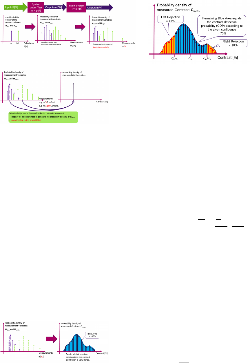
Figure 17. Probability density distributions of the possible measurements
after transferring back to the input domain
Figure 18. Picking up a random bright and a random dark measurement to
calculate the measured contrast between these two.
3. Calculate the measured contrast c
meas.
with the Weber contrast
equation (See figure 18).
Executing the above steps with many different measurement values,
the calculated contrasts c
meas.
form a distribution of the new random vari-
able C
meas.
. See figure 19 for an illustration.
We have to accept that the measured contrast has small derivations
ε
+
and ε
−
from the assumed input contrast c
in
. Depending on the appli-
cation either large or almost infinite small deviations can be chosen to be
acceptable.
Mathematical definition of CDP: Mathematically expressed we
define the contrast detection probability:
C
c
in
DP = Prob ((c
in
−ε
−
) < c
meas.
< (c
in
+ ε
+
)) (2)
Figure 20 shows an illustration on how the CDP value from eq. 2 can be
extracted from the measured contrast values.
Concluding, figure 21 summarizes the workflow for CDP measure-
ments as a block diagram.
Intensity dependent CDP
Given a defined reflectance contrast c
in
, CDP has a dependence on
many other variables:
Electrical System Configuration: Which is usually easy to keep con-
stant, e.g. by not changing exposure time and other registers.
Figure 19. Many randomly selected contrast measurements form a proba-
bility distribution, which belongs to the contrast’s random variable (C
meas.
).
Figure 20. Probability density distributions of the input and output of a
system. The system measures two reflectance differences and contains a
light source to physically illuminate the reflectances.
Temperature: Is controllable with medium difficulty, however more
than one temperature constant operation condition is typical.
Luminance: Is hard/impossible to control, as with a changing scene,
the system in input varies without control.
Given this motivation, the luminance dependency for given operat-
ing temperatures comes at first priority for investigations.
We consider an ideal image sensor, which produces for each detected
photon one electron and then counts the electrons one by one. The photon
flux obeys a Poisson statistic and for a given contrast c
in
the bright and the
dark patch of the contrast behave as Poisson noise generators:
µ
bright
= (1 + c
in
)µ
dark
(3)
P
µ
dark
(n) =
µ
dark
n
n!
e
−µ
dark
(4)
P
µ
bright
(n) =
µ
bright
n
n!
e
−µ
bright
(5)
with n as the number of photons in the given process.
In our ideal system we consider:
m[DN] = s(I, R) = 1
DN
e
· 1
e
ph
·I[ph.] ·R[%]
| {z }
generated Poissonian electrons
(6)
Starting with the definition of CDP, we can derive a theoretical fore-
cast for an ideal Poisson-only system:
C
c
DP = Pr ((c
in
−ε
−
) < c
meas.
< (c
in
+ ε
+
)) (7)
= Pr (c
meas.
< (c
in
+ ε
+
)) . . .
. . . −Pr (c
meas.
< (c
in
−ε
−
)) (8)
With ε
+
, ε
−
, c
in
as given, we can express c
meas.
depending on the
random variable based system model.
c
meas.
=
m
bright
m
dark
−1 (9)
=
e
bright
e
dark
−1 based on eq. 6 (10)
For the sake of notation: e
bright
and e
dark
and c
meas.
are Poisson
random variables and e
bright
and e
dark
and c
meas.
are their respective re-
alizations.
We can continue to derive CDP by:
Pr(c
meas.
< (c
in
+ ε
+
)) . . .
= Pr
e
bright
e
dark
−1 < (c
in
+ ε
+
)
(11)
= Pr
e
bright
< (c
in
+ ε
+
+ 1)e
dark
(12)
030-8
IS&T International Symposium on Electronic Imaging 2019
Autonomous Vehicles and Machines Conference 2019
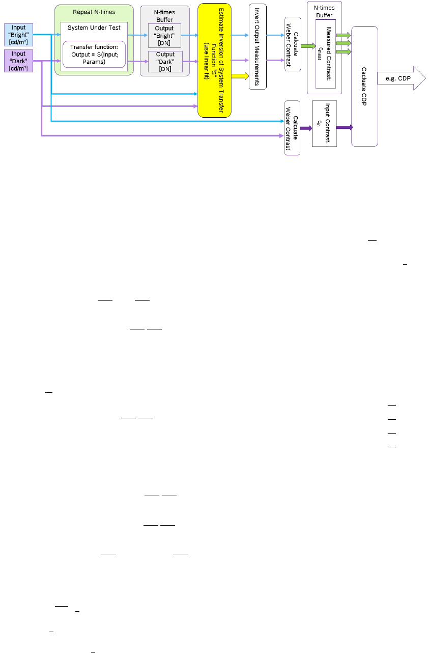
Figure 21. The summarized workflow for CDP measurement for any given system under test which results in one measurement value of CDP.
The above equation can only be fulfilled if e
dark
> 0, which is due to the
quantized nature of electrons and photons
e
dark
>= 1 (13)
To evaluate the full probability the summation over the bright intensity
need to be limited depending on the current dark patches electron count
(d = dark, b = bright):
. . . =
∞
∑
e
d
=1
b(c
in
+ε
+
+1)e
d
c
∑
e
b
=0
µ
b
e
b
e
b
!
e
−µ
b
·
µ
d
e
d
e
d
!
e
−µ
d
(14)
= e
−µ
d
e
−µ
b
∞
∑
e
d
=1
b(c
in
+ε
+
+1)e
d
c
∑
e
b
=0
µ
b
e
b
e
b
!
µ
d
e
d
e
d
!
(15)
This goes in the same methodology for the second term:
Pr(c
meas.
< (c
in
−ε
−
)) . . .
= Pr
e
b
e
d
−1 < (c
in
−ε
−
)
(16)
= e
−µ
d
e
−µ
b
∞
∑
e
d
=1
b(c
in
−ε
−
+1)e
d
c
∑
e
b
=0
µ
b
e
b
e
b
!
µ
d
e
d
e
d
!
(17)
Combined the CDP from eq. 8 gets into the form for Poisson-only
noise:
C
c
in
DP = Pr (c
m
< (c
in
+ ε
+
)) −Pr(c
m
< (c
in
−ε
−
)) (18)
= e
−µ
d
e
−µ
b
∞
∑
e
d
=1
b(c
in
+ε
+
+1)e
d
c
∑
e
b
=0
µ
b
e
b
e
b
!
µ
d
e
d
e
d
!
. . .
. . . −e
−µ
d
e
−µ
b
∞
∑
e
d
=1
b(c
in
−ε
−
+1)e
d
c
∑
e
b
=0
µ
b
e
b
e
b
!
µ
d
e
d
e
d
!
(19)
= e
−µ
d
e
−µ
b
∞
∑
e
d
=1
µ
d
e
d
e
d
!
b(c
in
+ε
+
+1)e
d
c
∑
e
b
=d(c
in
−ε
−
+1)e
d
e
µ
b
e
b
e
b
!
(20)
To be able to calculate this equation for larger electron or photon
counts we need to use the Stirling approximation:
n! ∼
√
2πn
n
e
n
(21)
logn! ∼
1
2
log2πn + log n
n
−loge
n
(22)
∼ n log n −n +
1
2
log2πn (23)
We include all exponential functions into their log approximation to get
the best numerical stability (including e
−µ
d
e
−µ
b
), and obtain:
f (e, µ) = exp
log
e
−µ
·
µ
e
e!
(24)
= exp
elog µ −e log e + e −
1
2
log2πe −µ
(25)
CDP =
∞
∑
e
d
=1
f (e
d
, µ
d
)
b(c
in
+ε
+
+1)e
d
c
∑
e
b
=d(c
in
−ε
−
+1)e
d
e
f (e
b
, µ
b
) (26)
For numerical evaluation we do not need to sum over all e
b
and e
d
, but
limit the summation to a certain number of standard deviations beyond of
which we consider the probability contribution as 0”. The range between
0 and 10 is however not excluded from summation as it does not yield to
computational efforts:
e
d,start
= max{0, µ
d
−N
d,start
·
√
µ
d
} (27)
e
d,stop
= max{10, µ
d
+ N
d,stop
·
√
µ
d
} (28)
e
b,start
= max{0, µ
d
−N
b,start
·
√
µ
d
} (29)
e
b,stop
= max{10, µ
d
+ N
b,stop
·
√
µ
d
} (30)
for the bright variables we also have to update the limits given by the
above deliberations that yield to the correct summing from eq. 20
e
b,start
= max{e
b,start
, d(c
in
−ε
−
+ 1)e
d
e} (31)
e
b,stop
= min{e
b,stop
, b(c
in
+ ε
+
+ 1)e
d
c} (32)
Here only µ
b
is an unknown variable and can be eliminated by using
the contrast definition:
µ
b
= (c
in
+ 1)µ
d
(33)
Further, the limits ε
−
and ε
+
are currently given as absolute limits w.r.t.
to the given contrast. While this a good choice to evaluate special contrast
detection tasks, these limits can also be expressed as relative percentages
to the incoming contrast, which allows a more generic evaluation:
c
in
+ ε
+
= c
in
+ δ
+
c
in
⇒ ε
+
= δ
+
·c
in
(34)
IS&T International Symposium on Electronic Imaging 2019
Autonomous Vehicles and Machines Conference 2019 030-9
And in the same way for ε
−
:
c
in
−ε
−
= c
in
−δ
−
c
in
⇒ ε
−
= δ
−
·c
in
(35)
Which gives in the above formula in the following way:
CDP =
∞
∑
e
d
=1
f (e
d
, µ
d
)
b(c
in
(1+δ
+
)+1)e
d
c
∑
e
b
=d(c
in
(1−δ
−
)+1)e
d
e
f (e
b
, µ
b
) (36)
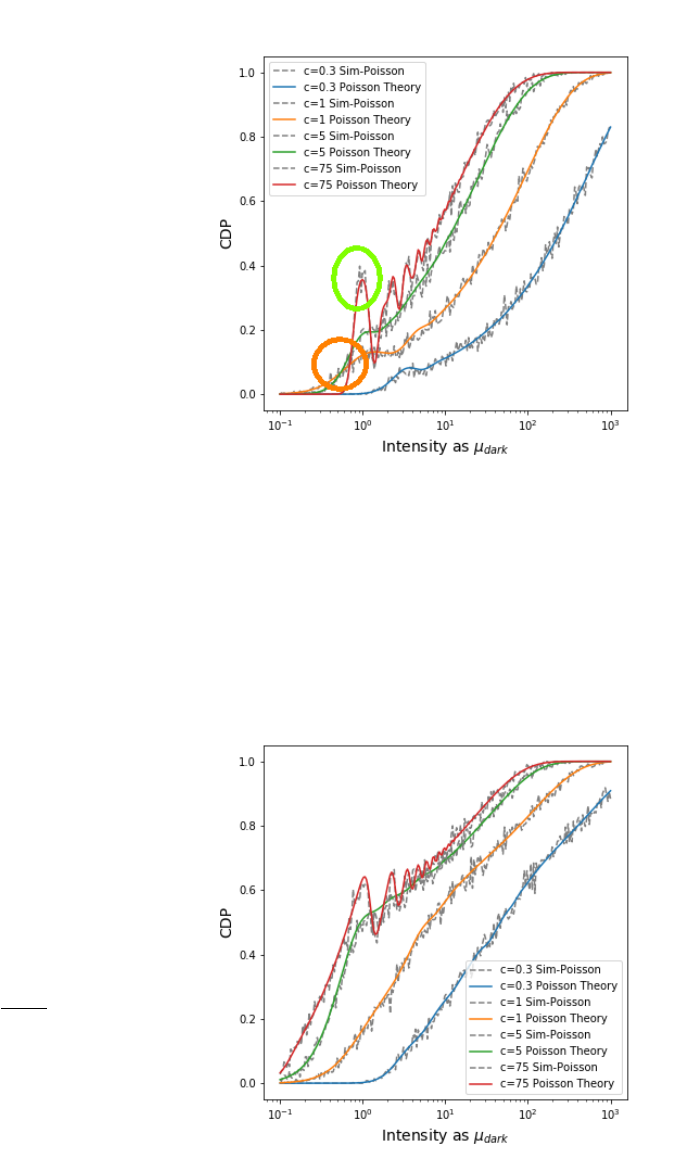
Figure 22 shows some plots of the derived equation against simu-
lations of this approach. It can be well observed that the simulation fits
the theoretical deliberations. We can observe that the ideal Poisson-only
noise system has a CDP that in general behaves as expected:
• Higher contrast leads to higher CDP
• More photons or electrons, leads to higher CDP
Further, CDP has the ability to detect the systems signal quantiza-
tion, especially if large contrasts are chosen. This is depicted in the green
circle and shows best for the c = 7500% Weber contrast. This yields to
a non-monotonic function and depending on the system under test this
effect can be based by each quantization process of the system: The pho-
tonic quantization, the photo-electrons or the ADCs. This property can be
used to analyze the systems behavior in detail.
As a side remark: For special experimental setups, e.g monochro-
matic light and well defined contrasts, this behavior could be used to mea-
sure basic physical constants.
We propose the following explanation of this behavior: CDP has
obviously a high value if the photon counts between bright and low signal
fits best to the input contrast. This behavior is attached to single photon
steps for intensities where the dark patch reaches an intensity of single
digit photon counts (or other quantization mechanisms). Utilization of
this behavior will be part of the further work.
For very low light intensities, CDP of the larger contrast is below the
CDP of the lower contrast. This a non-intuitive results but is explained by
the fact that at low light level a photon count of either one or zero photons
is present. As larger contrasts demand larger photon counts to fit into the
CDP confidence interval, compared to low contrasts the behavior makes
sense. To cross check this explanation, figure 23 shows that this behavior
goes indeed away if the lower acceptance limit is set to δ
−
= 90% for
example.
Non Summative Approximation Given the equations above and
the fact that Poissonian processes can be approximated by Gaussian Pro-
cesses if their expectation value is high enough it is also possible to get a
non-summative approximation by using a ratio of Gaussian processes.
CDP
Gauss
approximate by: c
in,Gauss
≈
e
b,Gauss
e
d,Gauss
−1 (37)
David Hinkley’s work can be used to derive the equations [3]. For this
work, only a simulation was considered which shows in figure 24 a signif-
icant derivation from the Poissonian approach. This hints that (as always)
Gaussian approximations shall only be used if their possible effects errors
have been evaluated in detail.
CDP approximation by SNR and EMVA1288
Having the above equations. We can start to include more complex
system models. For example the EMVA1288 standard gives us a model to
include some of the basic effects.
Figure 22. Intensity dependent CDP (δ
±
= 0.25) of different contrasts com-
pared to typical simualtion results (dashed lines). Green Circle: For large
contrasts, the quantization of the underlying signal which is based on pho-
tons and electrons becomes visible. Orange Circle: Due to a lack of signal
quants, large contrasts cannot be realized below a certain threshold. See
text for discussion.
Figure 23. Intensity dependent CDP (δ
−
= 0.9, δ
+
= 0.25) shows that CDP
curve crossing at low light does not happen in this case as described in the
discussion of this effect.
030-10
IS&T International Symposium on Electronic Imaging 2019
Autonomous Vehicles and Machines Conference 2019
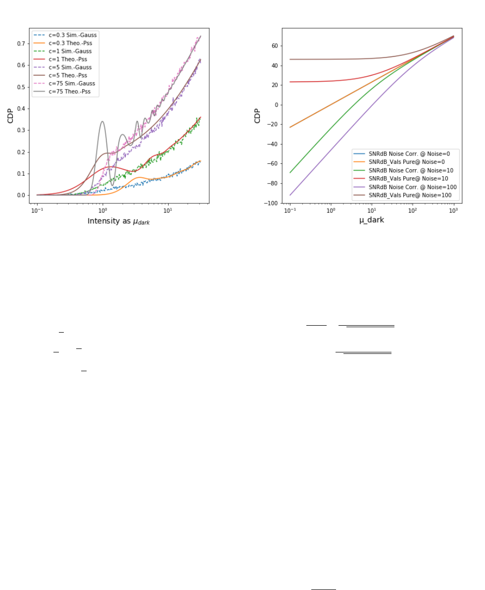
Figure 24. Intensity dependent CDP (δ
−
= 0.5, δ
+
= 0.5) by simulation with
a Gaussian approximation. The differences become clearly visible in the low
light domain around 1 to 10 photons.
We can use the Poissonian properties to set the above result into a
dependency to SNR:
σ
2
= µ as variance (38)
σ =
√
µ as standard deviation (39)
SNR =
µ
σ
=
√
µ (40)
SNR
dB
= 20 ·log
µ
σ
= 10 ·log(µ) (41)
Here we can choose either the bright or the dark number of electrons to
calculate the SNR. As the contrast detection usually demands for a detec-
tion of the dark patch, I propose to use the dark patches expectation value
to calculate the SNR. The results are already shown in the above plots.
If we want to calculate SNR in the domain of digital numbers DN we
need to include the possible more complex system function S and include
this into the above considerations.
Including Veiling Glare and Dark Current
If we want to include veiling glare and dark current we follow the
assumption from our Electronic Imaging AVM paper [1] that all further
contributions are additive Poisson noise sources. For the dark current and
the veiling glare this is obvious. For other electron generating sources our
last paper showed how they could be handled as Poisson sources as well.
As Poisson processes are additive we obtain for expectation value
and standard deviation the following:
Signal + Noise: σ
2
total
= σ
2
Signal
+ σ
2
Noise
(42)
Poissonian Variance: σ
2
total
= µ
total
= µ
Signal
+ µ
Noise
(43)
However, if we want to calculate SNR, we have to try to compensate
for the known noise sources otherwise the SNR gives large numbers even
in the absence of any signal. See figure 25 for an illustration. The fol-
lowing equations show how to calculate the noise corrected SNR for our
Figure 25. Intensity dependent SNR calculations for pure Poisson pro-
cesses. If the known noise sources are not considered, the SNR values give
large despite a noise degraded signal
given model:
SNR =
µ
Signal
σ
total
=
µ
total
−µ
Noise
p
µ
Signal
+ µ
Noise
(44)
SNR
dB
= 20 ·log
µ
total
−µ
Noise
p
µ
Signal
+ µ
Noise
!
(45)
A Poisson-only Systems’ CDP with given Noise
Extending our above approach for Poission systems to be polluted
with an additive noise, we also have to correct the noise mean value to
obtain a good CDP derivation. In full extend this should be done by in-
verting the system function S. To showcase the implication onto an ideal
noise deteriorated system, we can execute this task with the following
steps:
e
b
: bright signal including noise (46)
e
d
: dark signal including noise (47)
µ
N
: known expectation value of additive noise (48)
This allows us to rewrite to eq. 18 in the following way:
Prob(c
meas.
< (c
in
+ ε
+
)) . . .
. . . = P
e
b
−µ
N
e
d
−µ
N
−1 < (c
in
+ ε
+
)
(49)
= P (e
b
−µ
N
< (c
in
+ ε
+
+ 1)(e
dark
−µ
N
) (50)
= P (e
b
< ((c
in
+ ε
+
+ 1)(e
dark
−µ
N
) + µ
N
) (51)
= P (e
b
< (c
in
+ ε
+
+ 1)e
dark
−µ
N
(c
in
+ ε
+
)) (52)
IS&T International Symposium on Electronic Imaging 2019
Autonomous Vehicles and Machines Conference 2019 030-11
and similar for the second term:
Prob(c
meas.
< (c
in
−ε
−
)) . . .
= Prob
e
b
−µ
N
e
d
−µ
N
−1 < (c
in
−ε
−
)
(53)
= Prob (e
b
< (c
in
−ε
−
+ 1)e
d
−µ
N
(c
in
−ε
−
)) (54)
In analogy to the previous derivation, the Poisson limitation to values be-
tween 0 and ∞ has again an influence on the starting value of e
d
in the
summation:
e
b
≥ 0 (55)
⇒ 0 < (c
in
−ε
−
+ 1)e
d
−µ
N
(c
in
−ε
−
) (56)
e
d
>
µ
N
(c
in
−ε
−
)
(c
in
−ε
−
+ 1)
(57)
Thus we have starting values for e
d
for the high and low probability bor-
ders:
D
start,low
= d
µ
N
(c
in
−ε
−
)
(c
in
−ε
−
+ 1)
e (58)
D
start,high
= d
µ
N
(c
in
+ ε
+
)
(c
in
+ ε
+
+ 1)
e (59)
Combined we obtain for the CDP evaluation from eq. 8 the same
form but with adapted borders:
B
stop,low
= d(c
in
−ε
−
+ 1)e
d
−µ
N
(c
in
−ε
−
)e (60)
B
stop,high
= d(c
in
+ ε
+
+ 1)e
d
−µ
N
(c
in
+ ε
+
)d (61)
C
c
in
DP = Prob (c
meas.,noise
< (c
in
+ ε
+
)). . .
. . . −Prob (c
meas.,noise
< (c
in
−ε
−
)) (62)
=
∞
∑
e
d
=D
start,high
f (e
d
, µ
d
)
B
stop
∑
e
b
=0
f (e
b
, µ
b
). . .
. . . −
∞
∑
e
d
=D
start,low
f (e
d
, µ
d
)
B
stop,high
∑
e
b
=0
f (e
b
, µ
b
) (63)
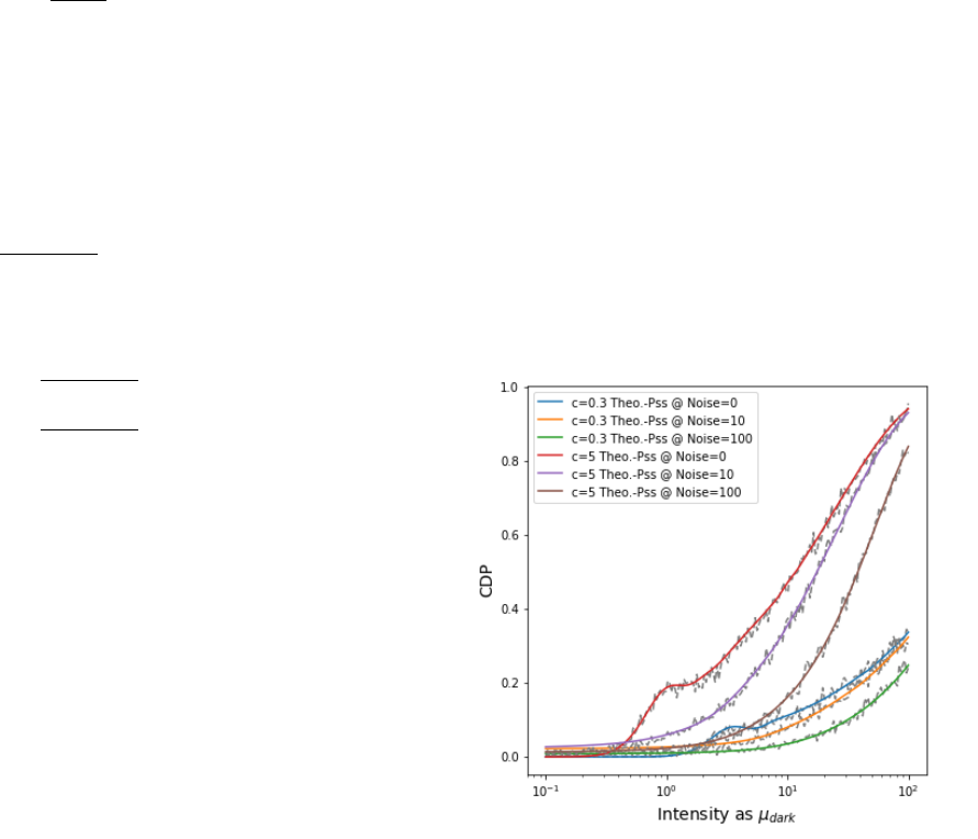
Figure 26 shows how CDP degrades if noise is added to the signal.
There are many different parametrization options for CDP. While some
implications have been discussed in the main text of this article, we leave
a further discussion to future work.
Figure 26. Intensity dependent CDP plots of c = 0.3 and c = 5 with added
noise in the strength of 0, 10 or 100 electrons.
030-12
IS&T International Symposium on Electronic Imaging 2019
Autonomous Vehicles and Machines Conference 2019
• SHORT COURSES • EXHIBITS • DEMONSTRATION SESSION • PLENARY TALKS •
• INTERACTIVE PAPER SESSION • SPECIAL EVENTS • TECHNICAL SESSIONS •
Electronic Imaging
IS&T International Symposium on
SCIENCE AND TECHNOLOGY
Imaging across applications . . . Where industry and academia meet!
JOIN US AT THE NEXT EI!
www.electronicimaging.org
imaging.org
