PivotTables - Excel 2019

January 2020

PivotTable reports (or PivotTables) make the data in your worksheets much more manageable by summarizing

the data and allowing you to manipulate it in different ways. PivotTables can be an indispensable tool when

used with large, complex spreadsheets, but they can be used with smaller spreadsheets as well. PivotTables in

Excel 2019 covers the basics of creating and manipulating PivotTables.

Overview of PivotTable Reports

Advantages of PivotTables

• Allows you to easily analyze and manipulate large sets of data

• With a PivotTable, you select only the fields that you wish to focus on

• You can quickly reposition any field on your PivotTable –

e.g. change it from a Vertical to a Horizontal position

• PivotTables allow you to easily add multiple summaries

– e.g. Sum, Average, Percentage of Total, etc without

writing a formula!

• It is impossible to harm your original data when you work

with a PivotTable because you are working with a “virtual

snapshot” of your data.

Getting Started

To create a PivotTable first enter the basic content into your Excel document or open an existing dataset.

1. Open Microsoft Excel 2019

2. Open the document excel_practice_file located in the Documents folder

If it appears, click on the yellow Enable Editing button at the top of the screen

3. Click on the PivotTable worksheet

Excel 2019

Part 7: PivotTables

Formatting data for use in a PivotTable

Formatting data for use in a PivotTable is an important first step!

The best way to format data for a PivotTable is as a list.

• A list is a series of columns, with each column displaying a category.

• Each row of the data should display a fact.

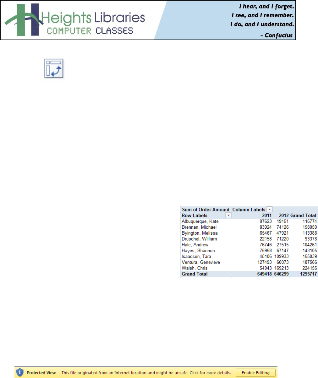
The example below contains sales information for a fictional car dealership. The data set, also called source

data, consists of 48 rows and 7 columns.

Each column displays a category of information: Salesperson, Brand, Year, Type, Model, Price and Date

Received. Each row displays a fact. For example, row 2 shows that the salesperson Kate Albuquerque sold a

2012 Ford Focus car for $19,151. The vehicle was received on August 4, 2012.

Source data should also not contain any gaps or extraneous information that will not be included in the

PivotTable. If a blank row or column is present, the complete data set will not be included in the PivotTable

report.

Using PivotTables to answer questions

Creating a PivotTable is an interactive way to quickly summarize and understand data. Using the example

above here are some questions about the data that a PivotTable can answer:

1. What is the amount sold by each salesperson?

2. What amount of car brand was sold by each salesperson?

3. What amount of product was sold in 2012 (or other year)?

4. How much of each car brand was sold?

5. How much of each car brand was sold in 2011 (or other year)?

Create a PivotTable

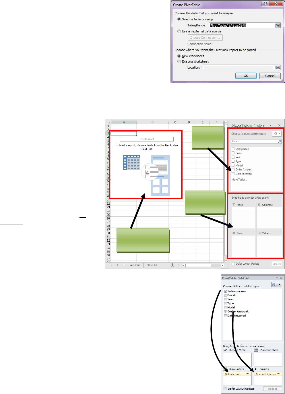
1. Click any single cell inside the data set.

2. Go to Insert tab → Tables group → PivotTable command

3. The Create PivotTable dialog box appears. Excel

automatically selects the data for you

NOTE: Always check that the correct data is selected. If it is not

selected properly, click and drag over the correct data in the

original data set.

When you click and drag over cells $ symbols appear around the

cell range. The $ symbols indicate an absolute cell reference and

are are needed for the PivotTable to populate.

4. Select the radio button next to New Worksheet

5. Click OK

A new worksheet is created with a blank PivotTable on the left. The Field List and the Layout Section appear

on the right side of the page.

The Field List displays the fields

available to you and mirrors the

columns from the source data.

The layout section is used to build the

PivotTable.

The Columns area displays column

headings in the PivotTable.

The Rows area creates row headings

in the PivotTable.

The Values area displays data as

functions in the body of the PivotTable.

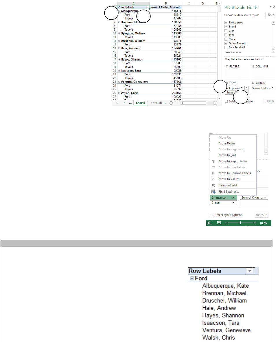
Add Fields to the PivotTable Report

To determine which fields to add to the PivotTable, first think back to your

question.

Question 1: What is the amount sold by each salesperson?

To view or summarize specific data, add the field that contains the data to

your PivotTable.

1. In the Field List, place a checkmark next to the Salesperson and

Order Amount fields.

The selected fields will be added to one of the four boxes in the Layout

Section. In this example, the Salesperson field is added to the Row

Labels box, and the Order Amount is added to the Values box. If a field is

not in the desired box, you can click and drag it to a different one.

Field

List

Blank

PivotTable

Layout

Section

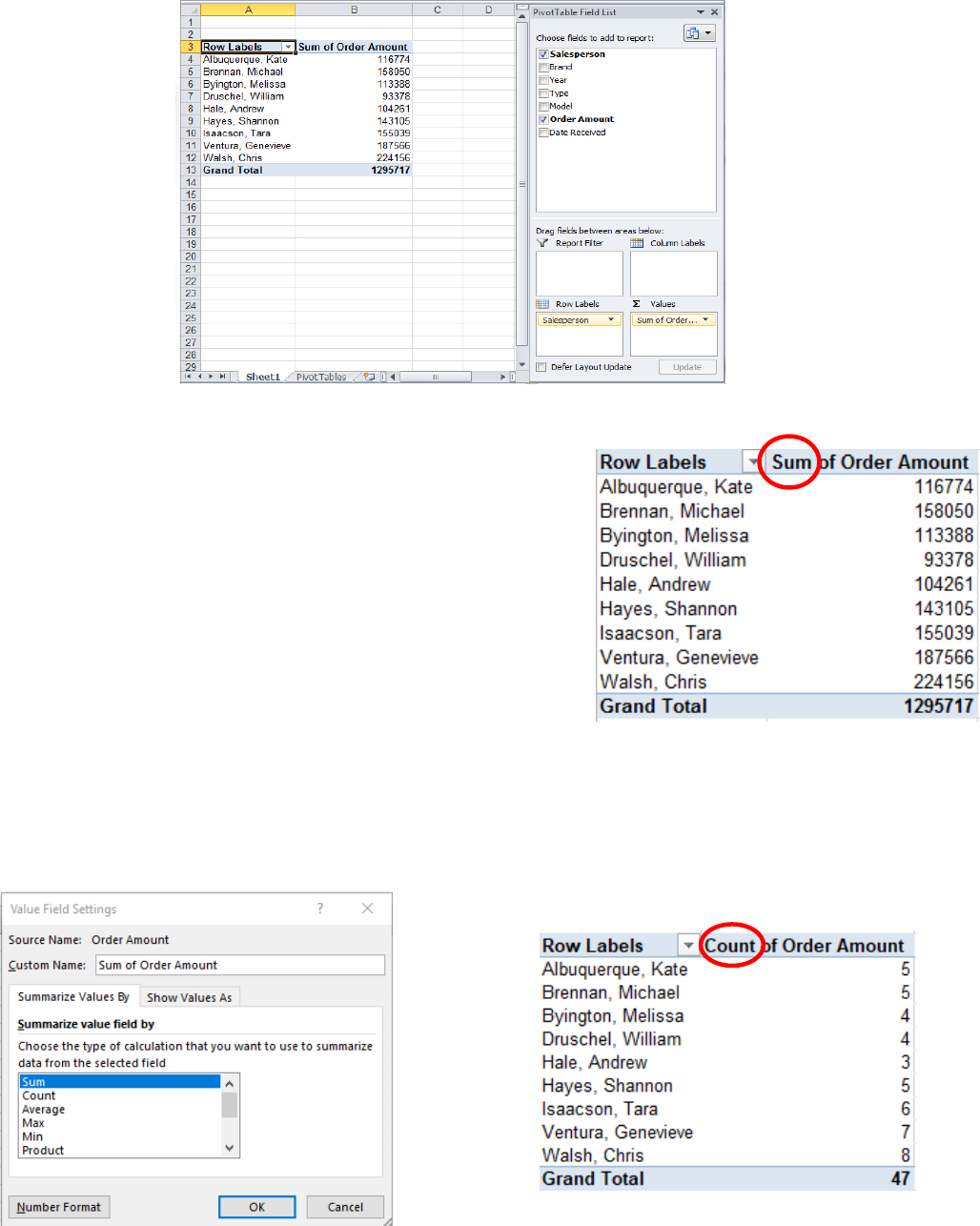
The PivotTable now shows the amount sold by each salesperson.

Change Value Calculation

By default Excel performs the most appropriate mathematical

calculation on the fields in the Values section of the PivotTable. In

the example on the right, Excel totals the values of Order Amount,

the field currently in the Values column, using the SUM function.

Totaling values is not the only option. Fields in the Values can be

changed to different functions such as COUNT, AVERAGE, MIN

and MAX. Instead of writing formulas in calculated fields,

use Summarize Values By command to quickly present values in

different ways.

Change the Value Calculation:

1. In the PivotTable, click on the value field, cell B3

2. Click the PivotTable Tools Analyze tab → Field Settings (Active Field group) →Field Settings

command →Summarize Values By tab

3. Select a function, such as COUNT, from the list and press OK

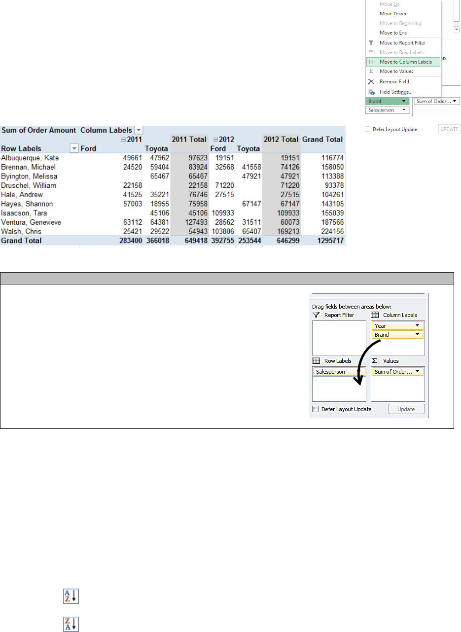
Pivoting Data

One of the best things about PivotTables is the ability to change the structure of the PivotTable to "pivot" (rotate)

the data. Pivoting data allows for the information to be viewed in many different ways.

Add Fields

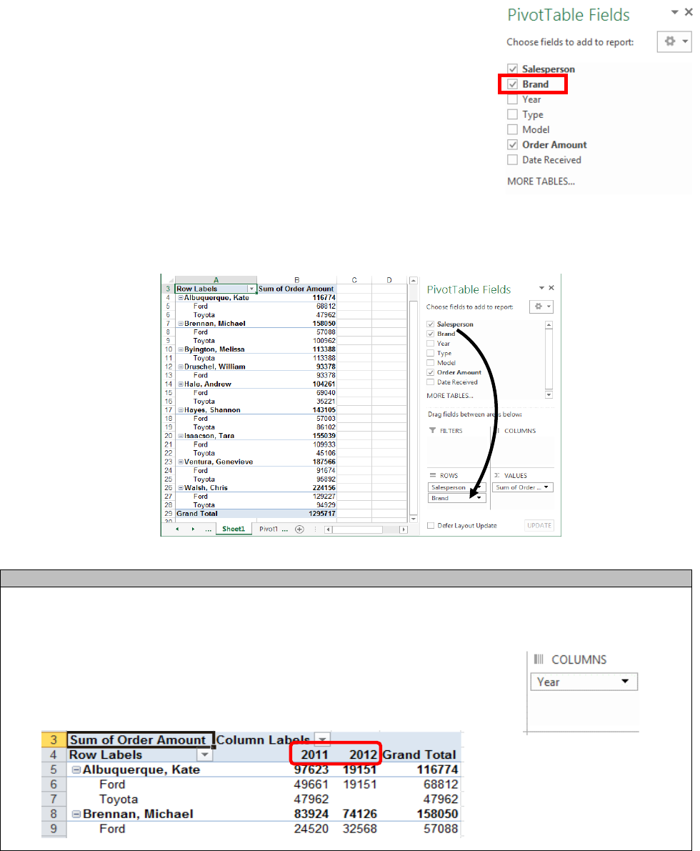
In the previous example the PivotTable was used to answer the question,

"What is the total amount sold by each salesperson?" Additional fields can be

added to the boxes in the Layout Section to answer additional questions.

Question 2: What amount of car brand was sold by each salesperson?

To answer the new question, place an additional field in the Row Labels box.

1. In the Field List, place a checkmark next to the Brand field.

The selected fields will be added to one of the four areas below the Field List.

In this example, the Brand field is added to the Row Labels area. If a field is

not in the desired area, click and drag it to a different section of the layout

section.

The PivotTable now shows the car brand amount sold by each salesperson.

Practice Exercise: Add Column Labels

So far, the PivotTable has only shown one column of data; Sum of Order Amount. In order to show multiple

columns, add fields to the Column Labels box.

1. On the sheet displaying your PivotTable, click and drag the Year field

from the Field List into the Columns box.

A second column displaying the Year displays in the PivotTable.

Rearrange Field Order

Fields dropped into the boxes in the

Layout Section appear in the order you

placed them into the area. For example,

the first field, Salesperson is the top-

most field in the Rows area of the

PivotTable. The second field, Brand,

appears next in the hierarchy order and

so on.

Change the field order to see the data in a different way

1. In the Layout Section click on the desired field

2. A menu appears, select one of the following options

o Move Up: Moves the field one space up

o Move Down: Moves the field one space down

o Move to Beginning: Moves the field to the top spot in the box

o Move to End: Moves the field to the bottom spot in the box

Practice Exercise: Rearrange Field Order

1. On the sheet displaying your PivotTable click on the Salesperson field in the Row Labels box

2. A menu appears; click Move Down

The hierarchy of rows in the PivotTable change and now display first

by Brand and then by Salesperson.

Change Field Location

Another way to see data from a different perspective is to turn Row Labels into

Column Headings (or vice versa).

1. On the sheet displaying your PivotTable click on the Brand field in the Row

Labels box

2. A menu appears; click Move to Column Labels

NOTE: Alternatively drag and drop headings from the Row Labels Box to the

Column Labels Box

Practice Exercise: Turn Column Label into Row Label

1. On the sheet displaying your PivotTable click and drag the

Brand field from the Column Labels box to the Row

Labels box

Sorting PivotTable Data

In Excel, PivotTable data can be sorted by any field located in the Row Labels or Column Labels boxes. Sorting

allows values to be sorted in alphabetic or numeric order.

Sorting Data

1. In the PivotTable report, click on the Row Labels or Column Labels header. For this example, click on

the text below the Row Labels Header.

2. Go to Data tab → Sort & Filter group → Sort commands

• Choose to perform an ascending sort (A to Z or smallest to largest number)

• Choose to perform a descending sort (Z to A or largest to smallest number)

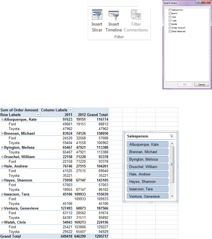
Filtering Data with Slicers

Filtering allows for a portion of the data to be viewed while hiding other data temporarily. In Microsoft Excel

2019, slicers were introduced to make filtering data easier and more interactive. Slicers provide buttons that you

can click to filter PivotTable data. In addition to quick filtering, the results are immediately visible with slicers.

Slicers also indicate the current filtering state, which makes it easy to understand exactly what data is shown in

a filtered PivotTable report.

To Filter Data Using Slicers:

1. Click on any cell in the PivotTable report

2. Go to Analyze tab → Filter group → Insert

Slicer

3. In the Insert Slicers dialog box, select the

desired field to be filtered, Salesperson

4. Click OK

The slicer will appear next to the PivotTable. Each selected item will be highlighted

in blue. In the example below, the slicer contains a list of all of the different salespeople,

and all of them are currently selected.

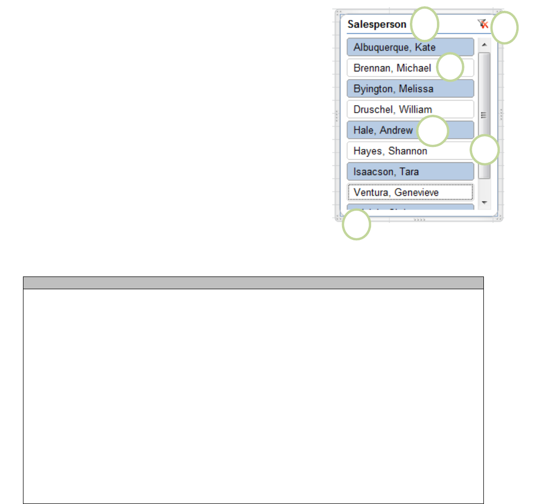
A slicer typically displays the following elements:

1. The slicer header indicates the category of the items in the slicer

2. A filtering button that is not selected displays in white and

indicates that the item is not included in the filter

3. A filtering button that is selected displays in blue and indicates

that the item is included in the filter.

4. The Clear Filter button removes the filter by selecting all items in

the slicer.

5. The scroll bar enables scrolling when there are more items than

are currently visible in the slicer.

6. Border moving and resizing controls allows the size and

location of the slicer box to be changed

NOTE: The Active Cell must be located in the PivotTable for the slicer

to be visible. If the slicer is not visible click on any cell in the

PivotTable

Practice Exercise: Using the Slicer

Only selected items in the slicer are visible in the PivotTable. When items are

selected or deselected items, the PivotTable will instantly reflect the changes. Try selecting

different items to see how they affect the PivotTable.

• Click on a salesperson’s name to select a single item

• To select multiple items, hold down the Control (Ctrl) key on your keyboard, click on

multiple items, then release the Ctrl key

• To select contiguous (right next to each other) items, click and drag the mouse over

various items

• To deselect a single item, hold down the Control (Ctrl) key on your keyboard, click on the

item, then release the Ctrl key

• Click the Clear Filter button to remove the filter and display all items in the PivotTable

Delete a slicer

A slicer can be deleted in one of the following ways:

Method 1:

1. Click the Clear Filter button

2. Press the delete key on the keyboard

Method 2:

1. Click the Clear Filter button

2. Right-click the slicer

3. Click Remove <Name of slicer>

Update the PivotTable

If changes are made to the source data the PivotTable does not automatically recognize the changes and

update the PivotTable. The PivotTable must be refreshed in order for the data to update.

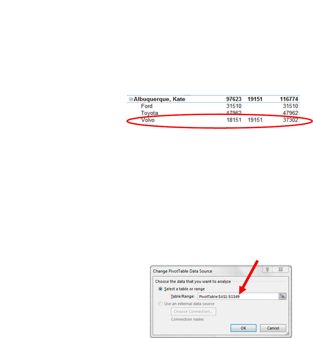
Edit the Source Data

Follow the steps below if edits to the source data do not change the size of the PivotTable

1. In the excel_practice_file select the PivotTables worksheet

2. Click in cell B2, type Volvo; press Enter to jump to cell B3

3. In cell B3, type Volvo

4. Press Enter

Refresh the PivotTable

1. In the excel_practice_file select the

worksheet that contains the

PivotTable (Sheet1)

2. Click in any cell in the PivotTable

3. Go to the Analyze tab → Data group

→ Refresh command

The data in the PivotTable changes and now displays the revised information

Update and Change the Size of the Source Data

If the size of your source data changes (add/delete columns and rows) or to select a different data source use

the Change Data Source command before refreshing the PivotTable

1. In the excel_practice_file select the PivotTables worksheet

2. Click in cell A49, type Lovelace, Ada; press Tab to jump to cell B49

3. In cell B49, type Tesla, press Tab to jump to cell C49

4. In cell C49, type 2020, press Tab to jump to cell D49

5. In cell D49, type Car, press Tab to jump to cell E49

6. In cell E49, type Model S, press Tab to jump to cell F49

7. In cell F49, type $74,490, press Tab to jump to cell G49

8. In cell G49, type 1/1/2020, press enter

Change Data Source

1. In the excel_practice_file select the

worksheet that contains the PivotTable

(Sheet1)

2. Click in any cell in the PivotTable

3. Go to the Analyze tab → Data group →

Change Data Source command

4. The Change PivotTable Data Source dialog

box appears

5. Click in the Table/Range box and change the

cell range to G49

The data in the PivotTable changes and now displays the information in the added row

Formatting

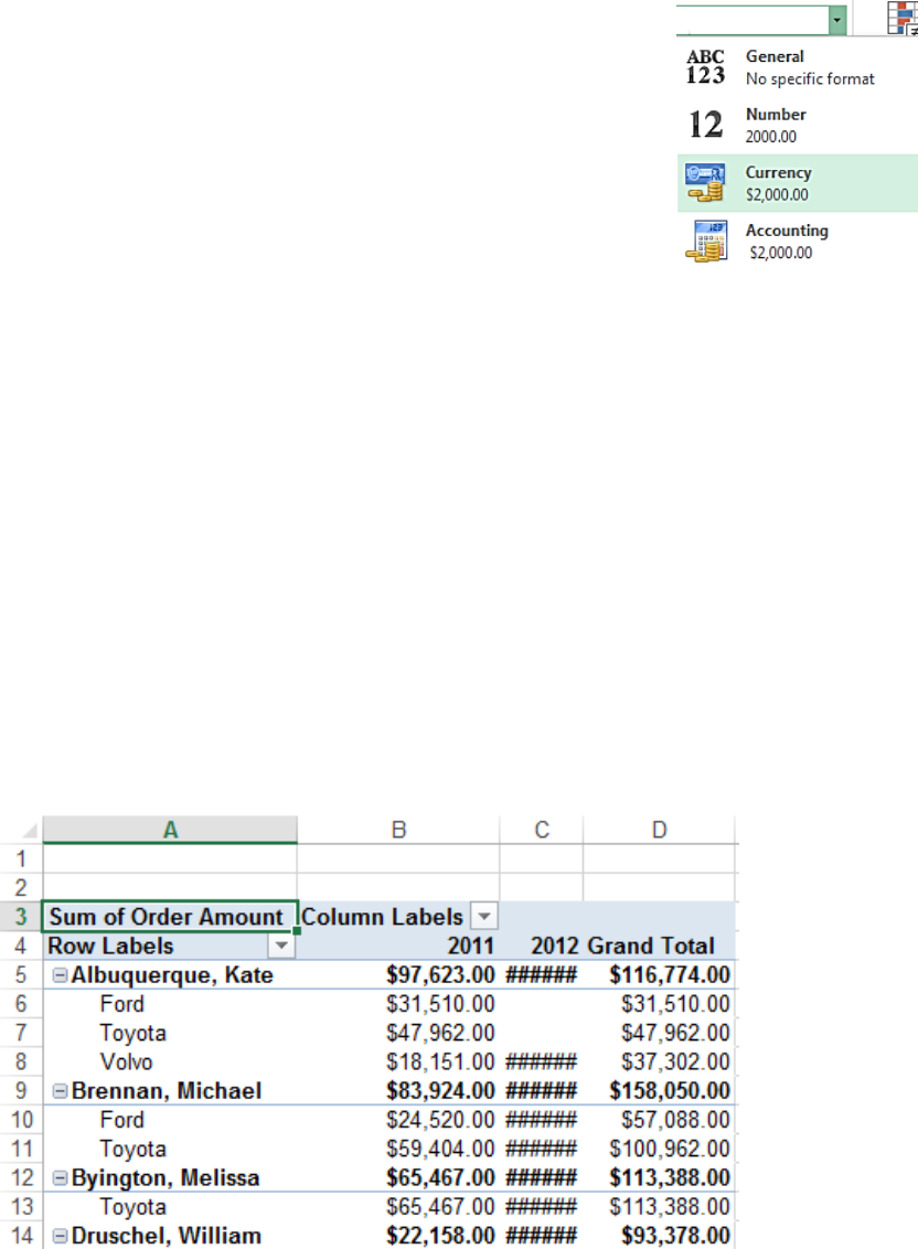
Changing Number Format

The PivotTable contains financial information but the current number format does not

display currency formatting. To change the number format on the spreadsheet:

1. Click and drag the mouse to select all of the cells in the PivotTable (B5-D31)

2. Go to the Home tab → Number group → Number Format drop down menu

3. Click on Currency

##### Error Message

#####, sometimes referred to as “railroad tracks”, is an Excel error message caused by several conditions:

• A number in a cell is too wide for the cell to display it.

• The formula in a cell produces a result that is too wide for the cell.

• There is a negative number in the cell that has been formatted for dates or times. Dates and times in

excel must be positive values.

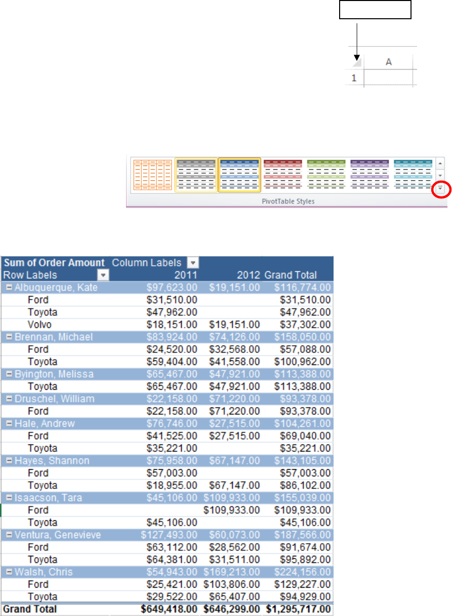
To fix the ##### error, place the cursor over the line between the two columns at the top of the worksheet.

When the cursor changes to a two-headed arrow with a line in between, double-click the mouse.

For example, in this worksheet:

1. Place your cursor between the C and D columns at the top of the worksheet.

2. When the cursor changes to a two-headed arrow with a line between, double-click the mouse

6. Repeat the steps above to widen the any other columns on the spreadsheet displaying the #####.

To adjust the width of all the columns at once:

1. To highlight the entire document (Ctrl+A) or Click the Select All button

2. Go to the Home tab → Cells group → Format command → AutoFit Column Width

Apply a style to format a PivotTable report

You can quickly change the look and format of a PivotTable by using a predefined PivotTable styles (or quick

styles).

1. Click anywhere in the PivotTable

report.

2. Go to the Design tab → PivotTable

Styles group

3. Click on the more button at the

bottom of the scroll bar to see the full menu of styles

4. Select the second thumbnail in the first row of the Medium format

NOTE: Formatting may disappear when other changes are made to the PivotTable

Select All

button