Chemical and optical properties of marine boundary layer aerosol particles of the mid‐Pacific in relation to sources and meteorological transport

JOURNAL OF GEOPHYSICAL RESEARCH, VOL. 101, NO. D3, PAGES 6931-6951, MARCH 20, 1996

Chemical and optical properties of marine boundary layer

aerosol particles of the mid-Pacific in relation to sources

and meteorological transport

P. K. Quinn, V. N. Kapustin, • and T. S. Bates •

NOAA, Pacific Marine Environmental Laboratory, Seattle, Washington

D. S. Covert 1

Department of Atmospheric Sciences, University of Washington, Seattle

Abstract. Incorporating the direct effect of tropospheric aerosol on climate into global

climate models involves coupling the optical properties of the aerosol with its physical and

chemical properties. This coupling is strengthened if the optical, physical, and chemical

properties of the individual aerosol components are known as well as how these properties

depend on the air mass source and synoptic scale meteorology. To relate properties of the

aerosol components to air mass sources over a wide range of meteorological conditions, two

long latitudinal cruises were conducted in the central Pacific Ocean from 55øN to 70øS.

Submicron non-sea-salt (nss) SO4 = aerosol averaged about 35 to 40% of the submicron ionic

mass as analyzed by ion chromatography and 6% of the total ionic mass, while supermicron

nss SO4 = aerosol contributed about 1% to the total ionic mass. About 1% of the remaining

total ionic mass was composed of methanesulfonate and 90% was sea salt. Ionic mass

fractions of nss SO4 = aerosol were highest in regions having the longest marine boundary

layer residence times or the largest source of marine or continental gas phase precursors. The

calculated scattering by nss SOft aerosol was highest in these same regions due to the

dependence of scattering on particle size and the concentration of nss SO4 = in the submicron

size range. The calculated scattering by submicron sea salt was similar to that of the nss SO4 =

aerosol, indicating that its contribution to scattering in the marine boundary layer can be

significant or even dominant depending on its mass concentration. Mass scattering efficien-

cies for nss SO4 = at 30% RH ranged from 4.3 to 7.5 m 2 g-1 and for submicron sea salt from

2 -1

3.5 to 7.7 rn g-. Mass backscattering efficiencies for nss SO4 = ranged from 0.41 to

2 1 2 1

0.58 rn g- and for submicron sea salt from 0.33 to 0.63 rn g-. These values fall within the

same range as others reported previously for the marine atmosphere.

1. Introduction

The direct effect of tropospheric aerosol on climate results

from the scattering by particles of incoming shortwave radiation

with a portion of it being reflected back to space. Defining

climate forcing as an externally imposed change on the Earth's

heat balance implies that a knowledge of the radiative properties

of both natural and anthropogenic aerosol components are

needed to calculate any change in the reflected flux, AF R, due to

an anthropogenic perturbation in aerosol loading or optical

properties. Parameters needed to calculate AFR include the mass

concentration of each aerosol chemical component, the mass

scattering efficiency, or the light scattering efficiency per unit

mass of each aerosol component j, {•sp j, and the fraction of

scattered light that is directed upward, [3. '•he latter quantity can

be approximated through the measurement of the backscattered

•Also at Joint Institute for the Study of the Atmosphere and

Ocean, University of Washington, Seattle.

Paper number 95JD03444.

0148-0227/96/95JD-03444505.00.

fraction, b, which is the fraction of scattered light that is

redirected to the backward hemisphere of the particle. Consider-

ation of b is useful as many values have been reported for a

variety of air mass types. The quantities b and [3 are equal for a

zenith Sun angle.

The dominant aerosol components present in the marine

boundary layer include nss SO4 = aerosol, sea-salt aerosol,

mineral dust, organic carbon species, and to a lesser extent,

elemental carbon. In general, a component is composed of

several chemical elements, compounds, or ions. Non-sea-salt

SO4 = aerosol found in the marine boundary layer can have

marine, volcanic, and anthropogenic sources. Therefore it can be

part of the natural aerosol system or it can be an anthropogenic

perturbation of that system such that it will contribute to climate

forcing by tropospheric aerosol. It may be derived from the

oxidation of biogenic dimethylsulfide (DMS) which is emitted

from the ocean surface [Andreae, 1986; Bates et al., 1987], the

oxidation of volcanic gas phase SO 2 [Stoiber et al., 1987], or the

long range transport of anthropogenic air masses from continen-

tal regions [Quinn et al., 1990]. The latter may involve transport

through the free troposphere [Clarke, 1993]. Impactor measure-

ments indicate that nss SO4 = aerosol mass is concentrated

primarily in the 0.1 to 1.0 pm diameter size range [e.g., Whitby,

6931

6932 QUINN ET AL.: CHEMICAL AND OPTICAL PROPERTIES OF AEROSOLS

1978; Savoie and Prospero, 1982; Pszenny et al., 1989; Quinn

et al., 1993].

Sea-salt aerosol is derived from the evaporation of seaspray

droplets and hence is part of the natural marine aerosol system.

It dominates the mass of the supermicron particle size range in

the marine boundary layer but can also contribute a significant

amount of mass to the submicron size range [O'Dowd and

Smith, 1993]. The number concentration of sea-salt aerosol in

the submicron size range is small, however, often contributing

only 4 to 10% of the total number [Mclnnes et al., 1995a].

Particles containing mineral dust are produced by the

weathering of soils and rock as well as through industrial and

agricultural practices. These particles have diameters ranging

from less than 1 •m to 100 •m. Those with diameters up to

about 4 •m can be transported over long distances [Merrill et

al., 1994], so that at times they can contribute a significant

amount of mass to the marine boundary layer aerosol.

Organic carbon compounds in the marine boundary layer can

have natural marine and terrestrial sources as well as anthropo-

genic sources. The ocean is a source of particulate organic

species through the direct injection of biogenic surfactants from

bubble bursting processes [Monahan, 1986] or the emission of

gas phase precursors [Plass-Dulmer et al., 1995]. Gaseous

organic carbon species emitted by natural terrestrial sources and

anthropogenic combustion may be transformed to the aerosol

phase through oxidation or condensation and transported over

long distances to the marine atmosphere. To date, the organic

content of marine aerosol particles has not been well quantified

or speciated. The few data that have been reported indicate that

carbon-containing species can make up 4 to 15% of the total

marine aerosol mass with more than 90% of this mass in the

form of organic carbon [Rau and Khalil, 1993].

From the number-size distribution and an estimation of the

particle density and refractive index, the scattering and backscat-

tering coefficients, Osp and Ubsp, can be calculated for the total

aerosol with Mie theory. In addition, knowledge of the chemical

mass-size distribution of each aerosol component j allows for

the calculation of the scattering coefficient of that component,

or Usp, j. The scattering coefficient for the components then can

be used to determine the fractional contribution of the compo-

nent to scattering and backscattering by the aerosol as a whole

and to calculate the mass scattering efficiency of the component.

For aerosol component j the mass scattering efficiency is

defined as the component's scattering increment per mass

increment or

0 Osp,j ( 1 )

IgsP'/ - 0m. '

If the total mass of component j is not known, an individual

species can be used as an indicator for that component. For

example, the nss SO 4- ion can be used as an indicator to

represent the complete nss SO 4- aerosol component composed

of nss SO 4- and the mass of NH4* and H20 that is universally

associated with it under most atmospheric conditions.

The magnitude of the scattering and backscattering coeffi-

cients of each aerosol component depends on its size dependent

mass (or volume) concentration. The dependence of the scatter-

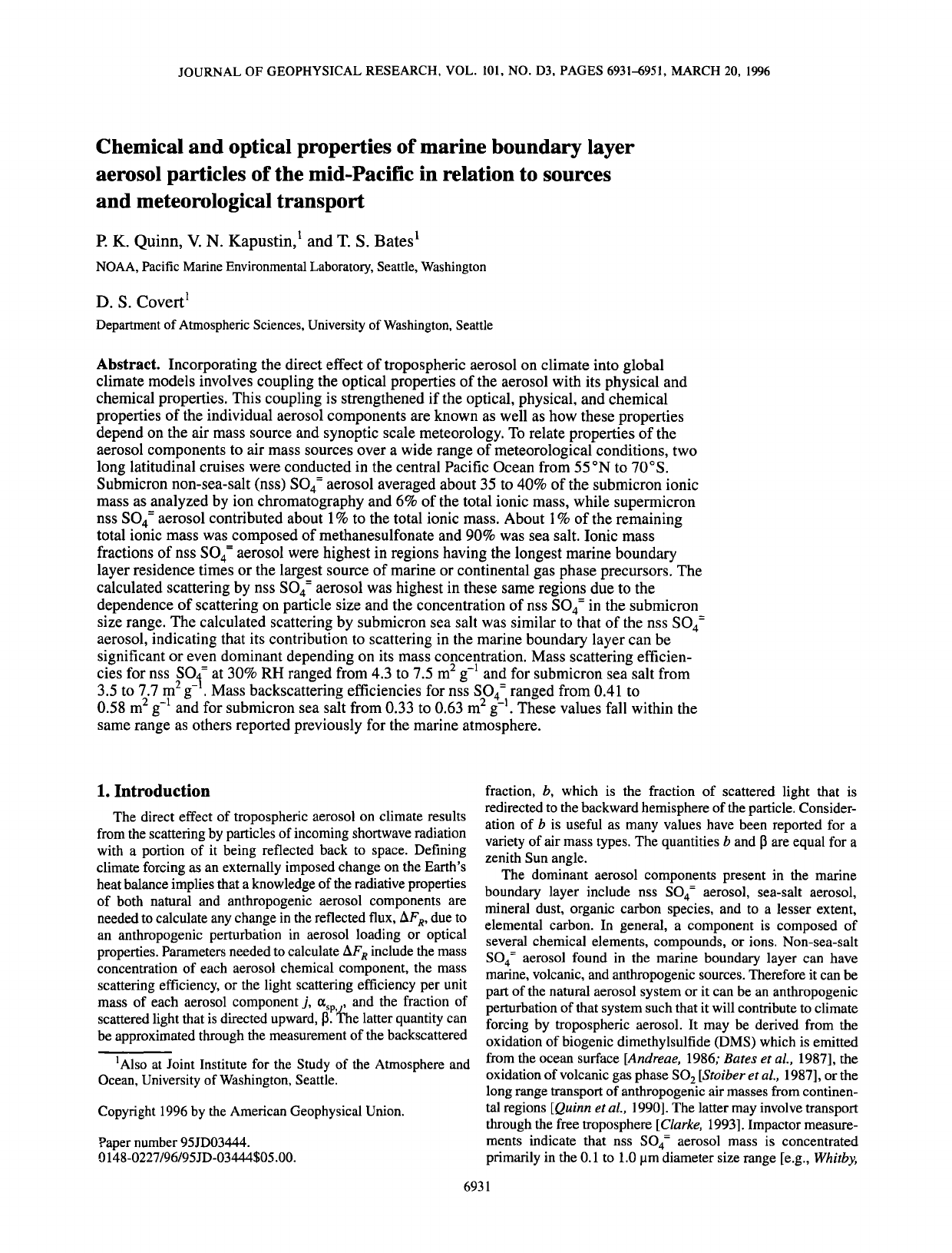
ing coefficient on particle size is shown in Figure 1 for a

wavelength of 0.55 Bm, particles of unit volume, and a refractive

index of 1.5-10-7i, which is near that of (NH4)2SO 4 and sea salt

at low relative humidity. For these conditions, on a mass or

volume basis, the scattering efficiency is lognormally distributed

with the most efficient size range for scattering occurring

between particle diameters of 0.2 and 1.0 Bm.

What this implies for scattering by atmospheric aerosols is

shown by comparing these calculated scattering efficiency size

distributions with size distributions of the atmospheric aerosol.

Figure 1 shows two measured size distributions, one from a

marine air mass (solid line with symbols) and one from a

continentally influenced air mass (dashed line with symbols).

For the marine case, the minimum between the submicron and

supermicron modes coincides with the maximum in the scatter-

ing distribution. Therefore scattering by the total aerosol will be

affected by both modes but largely controlled by the super-

micron mode due to its large mass concentration, in spite of the

decrease in the scattering coefficient with size. For the continen-

tal case, the submicron mode will have a larger effect on

scattering by the aerosol as a whole than it did in the marine

case, as its peak diameter is shifted toward the maximum in the

scattering distribution. The supermicron mode will have a

smaller effect, however, as it has a lower mass concentration.

Clearly, both the geometric volume mean diameter and the mass

concentration of an atmospheric aerosol component will

strongly affect the amount the component contributes to

scattering by the whole aerosol.

For a given aerosol mass concentration and number distribu-

tion, differences in chemical composition also will affect

scattering by the total aerosol. This effect is such that for

diameters between 0.2 and 0.3 gm, an increase in the real

portion of the refractive index from 1.4 (50% H2SO 4 / 50%

H20 ) to 1.5 ((NH4)2SO4) yields a 60% increase in O•p and a 50%

increase in Ubs p [Marshall 1994]. As a result, the degree of

neutralization of nss SO4 = aerosol by NH 3 (g) will affect

scattering by the total aerosol. Similarly, the addition of a

significant amount of sea salt, which also has a refractive index

near 1.5, to a H2SO 4 aerosol also will affect scattering by the

total aerosol. The backscattered fraction shows the largest

sensitivity to change in refractive index at a diameter near

1.0 pm [Marshall, 1994]. Hence b will change with wind speed

as the mass distribution of sea-salt aerosol changes above and

below 1.0 gm. The optical properties of the aerosol also will be

affected by the incorporation of a small amount of a strong

absorber such as elemental carbon. Such changes have yet to be

quantified, however.

As indicated in the above discussion, the size dependent

chemical composition and mass concentration of tropospheric

aerosol components determine the optical properties of the

aerosol. These size dependent aerosol parameters are, in turn, a

result of synoptic scale meteorology and air mass sources. Data

collected during two Radiatively Important Trace Species

(RITS) cruises in the central Pacific Ocean have allowed for an

analysis of the effect of meteorological transport on the number

distribution [Covert et al., 1995]. The number concentration in

the Aitken (particle diameter, Dp, of 0.01 to 0.1 gm) and

accumulation (Dp of 0.1 to 0.5 pm) modes was found to depend

on the relative importance of the transport of ultrafine

(<0.01 pm) and Aitken particles from the free troposphere to the

marine boundary layer versus the aging of Aitken and accumula-

tion mode particles within the boundary layer due to vapor

condensation and cloud processing. In middle- and high-latitude

regions, subsidence from the free troposphere was frequent and

aging processes were limited by the short amount of time the

aerosol spent in the boundary layer. As a result, the Aitken mode

dominated the number distribution but contributed little to total

mass or light scattering. In the tropics, more time in the bound-

ary layer and more frequent clouds led to size distributions with

roughly equal number in the Aitken and accumulation modes

and, accordingly, a greater mass in the accumulation mode.

QUINN ET AL.: CHEMICAL AND OPTICAL PROPERTIES OF AEROSOLS 6933

1.0x10-5

8.0X10-6

6.0x10-6

4.0x10-6 -

2 0x10 -6 -

001

i i ! . i , 1,1 ! [ ! ! , i ill I I . , ! . I.

Osp V

o =1.3 j• • marine - 0.8

_ sg / \ ...... continental

_ 0.6

.. -. • - 0.2

........... I , -'i•, O0

01 1 10

Dgv(,U,m)

Parameter Marine Continental

accumulation coarse model accumulation coarse mode

mode mode

V, gm 3 cm -3 0.14 7.34 0.49 4.82

Dg•, gm 0.197 2.72 0.295 2.43

o•g 1.31 1.82 1.33 1.82

Figure 1. Plain solid and dashed lines represent the scattering coefficient as a function of geometric mean

volume diameter D

index of 1.5-10-Yi, a• estimated from a Mie calculation using a wavelength of 0.55 pm, a particle refractive

a total particle volume of 1 pm 3 cm -3. The calculation was done for geometric standard

deviations, o , of 1.3 and 1.8. Solid and dashed lines with symbols represent volume concentrations as a function

of D._ v calcul•t•ed from measured number-size distributions during one of the Radiatively Important Trace Species

(RITES 93) cruises. These size distributions are averages over impactor samples collected in marine (solid line,

2øN) and continental (dashed line, 27øN) air masses. DISTFIT (version 1.10, TSI) was used to calculate the

modal parameters.

A similar data analysis of meteorology and aerosol chemistry

should reveal the effect of air mass sources and meteorological

transport on the relative concentrations and mass distributions

of the individual aerosol components. Therefore the same two

RITS data sets have been analyzed to define the relationship

between aerosol optical properties and source-determined

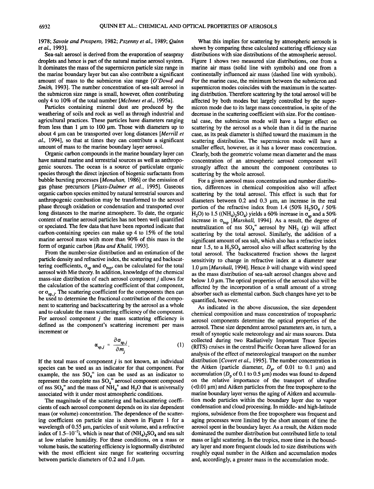
chemical properties. The RITS 93 cruise traveled from 70øS to

55 øN along 140øW from March to May 1993 (Figure 2a). The

RITS 94 cruise (Figure 2b) followed the same track but in the

opposite direction from November 1993 to January 1994.

Presented here are the results from these data sets which (1)

relate synoptic scale meteorology and air mass sources to

aerosol size dependent chemical composition in the marine

boundary layer, (2) define the mass fraction of each aerosol

ionic component present, (3) relate the ionic mass fraction of

each aerosol component to its contribution to scattering and

backscattering by the aerosol as a whole, and (4) determine the

mass scattering efficiency for the ionic aerosol components. In

addition, these results are compared to those reported from

previous studies of marine air masses.

2. Methods

2.1. Measurements

The RITS 93 and RITS 94 cruise tracks are shown in Figures

2a and 2b, respectively. Sample air for all measurements was

drawn through a 6-m heated sample inlet and dried to a relative

humidity (RH) near 30%. The top of the inlet was 18 m above

the ocean surface and 10 m forward of the ship's stack.

The number distribution between 0.02 and 0.6 pm was

measured every 10 min with a differential mobility analyzer

(DMA) (TSI model 3071 [Liu and Pui, 1975]) in conjunction

with a condensation particle counter (CPC) (TSI model 3760).

A Kr 85 charge neutralizer (TSI model 3077) was used to

produce an equilibrium charge distribution. An impactor with a

50% cutoff diameter of 0.7 pm bounded the upper limit of the

aerosol at the inlet and facilitated the inversion algorithm. A

minimum of 1000 particles was counted in each size increment,

yielding an uncertainty of about 3% for one standard deviation,

assuming Poisson counting statistics. The number concentration

was corrected for the counting efficiency of the particle counter

[Zang and Liu, 1991] and diffusion losses in the DMA

[Reineking and Porstendorfer, 1986]. A Boltzmann-Fuchs

equilibrium charge distribution was assumed to be present on

the particles analyzed. The number-mobility distribution was

inverted to a number-size distribution using an algorithm similar

to that provided by the manufacturer [Keady et al., 1983].

The number distribution between 0.6 and 9.6 }am was

measured with an aerodynamic particle sizer (APS) (TSI model

3300 [Baron, 1986]). The calibration of the APS was checked

between cruises with polystyrene latex spheres and found to be

within 1% of the manufacturer's calibration. The APS was

6934 QUINN ET AL.: CHEMICAL AND OPTICAL PROPERTIES OF AEROSOLS

(a)

..... RITS 1993

'-e.

160 ø 180 ø 160 ø 140 ø 120 ø 1 O0 ø 80 ø 60 ø

60øN

20øN

20øS

40 ø

- 60oS

rnb

73 ø

40ow 960 1000 1040

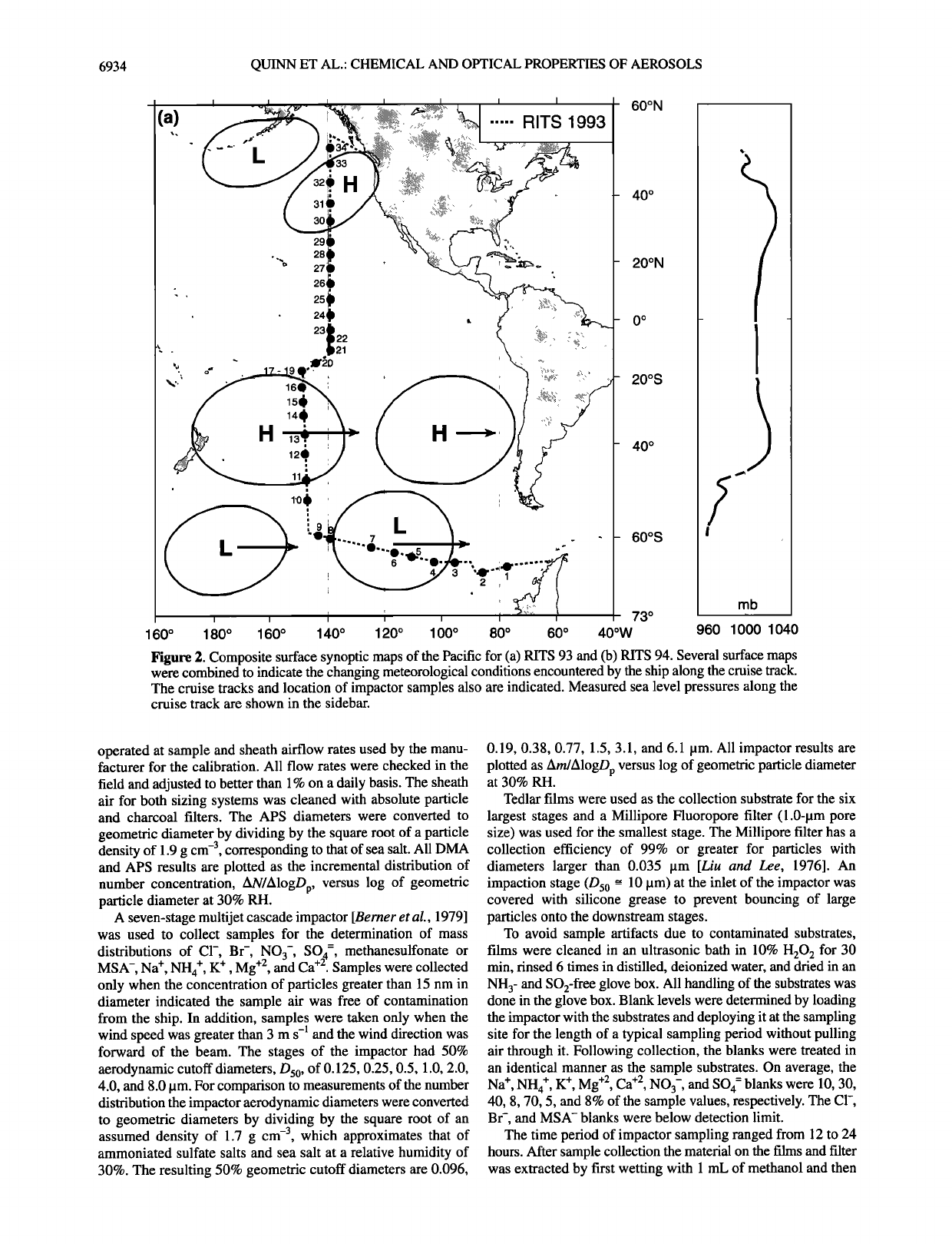
Figure 2. Composite surface synoptic maps of the Pacific for (a) RiTS 93 and (b) RITS 94. Several surface maps

were combined to indicate the changing meteorological conditions encountered by the ship along the cruise track.

The cruise tracks and location of impactor samples also are indicated. Measured sea level pressures along the

cruise track are shown in the sidebar.

operated at sample and sheath airflow rates used by the manu-

facturer for the calibration. All flow rates were checked in the

field and adjusted to better than 1% on a daily basis. The sheath

air for both sizing systems was cleaned with absolute particle

and charcoal filters. The APS diameters were converted to

geometric diameter by dividing by the square root of a particle

density of 1.9 gcm -3, corresponding to that of sea salt. All DMA

and APS results are plotted as the incremental distribution of

number concentration, AN/AlogDp, versus log of geometric

particle diameter at 30% RH.

A seven-stage multijet cascade impactor [Berner et al., 1979]

was used to collect samples for the determination of mass

distributions of CI-, Br-, NO3-, SOn =, methanesulfonate or

MSA-, Na +, NH4 +, K + , Mg +2, and Ca . Samples were collected

only when the concentration of particles greater than 15 nm in

diameter indicated the sample air was free of contamination

from the ship. In addition, samples were taken only when the

wind speed was greater than 3 m s -• and the wind direction was

forward of the beam. The stages of the impactor had 50%

aerodynamic cutoff diameters, Ds0, of 0.125, 0.25, 0.5, 1.0, 2.0,

4.0, and 8.0 lam. For comparison to measurements of the number

distribution the impactor aerodynamic diameters were converted

to geometric diameters by dividing by the square root of an

assumed density of 1.7 gcm -3, which approximates that of

ammoniated sulfate salts and sea salt at a relative humidity of

30%. The resulting 50% geometric cutoff diameters are 0.096,

0.19, 0.38, 0.77, 1.5, 3.1, and 6.1 gm. All impactor results are

plotted as Am/AlogDp versus log of geometric particle diameter

at 30% RH.

Tedlar films were used as the collection substrate for the six

largest stages and a Millipore Fluoropore filter (1.0-gm pore

size) was used for the smallest stage. The Millipore filter has a

collection efficiency of 99% or greater for particles with

diameters larger than 0.035 gm [Liu and Lee, 1976]. An

impaction stage (Ds0 • 10 gm) at the inlet of the impactor was

covered with silicone grease to prevent bouncing of large

particles onto the downstream stages.

To avoid sample artifacts due to contaminated substrates,

films were cleaned in an ultrasonic bath in 10% H202 for 30

min, rinsed 6 times in distilled, deionized water, and dried in an

NH 3- and SO2-free glove box. All handling of the substrates was

done in the glove box. Blank levels were determined by loading

the impactor with the substrates and deploying it at the sampling

site for the length of a typical sampling period without pulling

air through it. Following collection, the blanks were treated in

an identical manner as the sample substrates. On average, the

Na +, NH4 +, K +, Mg +2, Ca +2, NO3-, and SO4 = blanks were 10, 30,

40, 8, 70, 5, and 8% of the sample values, respectively. The CI-,

Br-, and MSA-blanks were below detection limit.

The time period of impactor sampling ranged from 12 to 24

hours. After sample collection the material on the films and filter

was extracted by first wetting with 1 mL of methanol and then

QUINN ET AL.: CHEMICAL AND OPTICAL PROPERTIES OF AEROSOLS 6935

. 13• 14 • :

,%..::'... ø• . . . 161F' .... .... ::..

I I I I I I 1

160 ø 180 ø 160 ø 140 ø 120 ø 1 O0 ø 80':' 60':'

• 60ON

- 40 ø

- 20ON

- 0 o

20øS

40 ø

60øS

73 ø

40øW

960

rnb

1000 1040

Figure 2. (continued)

adding 5 mL of distilled deionized water and sonicating for 15

min. Extracts were analyzed by ion chromatography. The cation

analysis was done with a Dionex CS-12 column, 20-mM MSA

eluant, and deionized water regenerant using the self-regenerat-

ing Dionex CSRS-1 suppressor system. Anion analysis was

done with a Dionex AS-4A column, 0.76-mM NaHCO3/2.0-mM

Na2CO 3 eluant, and 12.6-m]V/H2SO 4 regenerant. MSA-analysis

was performed with a Dionex AS-4 column, a 5-mM NaOH

mobile phase to elute the weak organic acids followed by 100-

mM NaOH to elute the stronger acids, and 12.6-mM H2SO 4

regenerant. Non-sea-salt SO4 = concentrations were calculated

from Na + concentrations and the molar ratio of sulfate to sodium

in seawater of 0.0603 [Holland, 1978].

Measurements of the scattering coefficient, Osp,meas, were

made at a wavelength of 0.55 gm with an integrating nephelom-

eter [Bodhaine et al., 1991] over a scattering angle, 0, where

8 ø _< 0 _< 168 ø. Every 3 to 4 days the nephelometer was cali-

brated with the Rayleigh scattering value of CO 2 of 2.61 times

air and was zeroed with particle-free air.

Ancillary measurements included surface temperature, dew

point, wind speed, wind direction, and rawinsonde data.

Rawinsonde balloons were launched at standard times of 0000

and 1200 GMT. Air mass back trajectories were calculated for

up to 12 days using the hybrid single-particle Lagrangian

integrated trajectories model, HY-SPLIT, based on wind fields

generated by the medium-range forecast (MRF) model [Draxler,

1992]. Trajectories were terminated at the ship's location at

1000 mbar. Surface and upper air maps were obtained from the

National Weather Service archives to aid in the analysis of

meteorological conditions and air motion.

2.2. Model Calculations

2.2.1. Calculation of scattering and backscattering by the

total aerosol. The first step in calculating the light scattering

(backscattering) due to each aerosol component was to test the

ability of the Mie model to estimate accurately the scattering

characteristics of the aerosol as a whole over all particle sizes

and chemical components. To calculate the scattering due to the

total aerosol, the Mie model was applied to the measured

number distributions and the density and refractive index were

derived from the measured chemical composition. These

calculated scattering values then were compared to those

measured directly with the nephelometer. The results of the

comparison are discussed in section 3.4. Backscattering values

also were calculated to derive the backscattered fraction b.

The model calculations described briefly here are presented

in greater detail in Marshall [ 1994]. The scattering and back-

scattering efficiencies, Qsp and Qbsp, were obtained at discrete

particle sizes by integrating over the scattered intensity function

from 8 ø to 168 ø and 90 ø to 168 ø, respectively [Bohren and

Huffman, 1983]. These efficiencies were then summed over the

measured number distribution to yield the calculated scattering,

Osp,calc, and backscattering, Obsp,calc , coefficients using

6936 QUINN ET AL.: CHEMICAL AND OPTICAL PROPERTIES OF AEROSOLS

Osp;bsp: E Qsp;bsp (Oi,g',n) •Z •

AlogD i

4 AlogD i

(2)

where D i is the geometric diameter of the measured particle size

increment. Particles are assumed to be spherical, 3, is the

wavelength of incident light, and n is the particle refractive

index. Even though the particles are subjected to decreasing RH

as they pass through the heated sampling inlet, they are expected

to remain spherical solution droplets due to hysteresis in the

crystallization of the hygroscopic nss SO4 = and sea-salt aerosol

components. Therefore the uncertainty associated with the

assumption of spherical particles is expected to be small.

The number distributions used in (2) were obtained by

averaging the measured DMA and APS data over the impactor

sampling times. Particles were assumed to be homogeneous

spheres distributed as an external mixture of two components:

a nss SO4 = aerosol composed of nss SO4 =, NH4 +, and H20, and

a sea-salt aerosol composed of Na +, K +, Mg +2, Ca +2, CI-, Br-,

NO3-, and sea-salt SOft. The assumption of an external mixture

is supported by the clear size separation of nss SO4 = and sea-salt

aerosol into the submicron and supermicron size ranges (see

section 3.2) and by individual particle analysis with an analytical

electron microscope [Mclnnes et al., 1995a].

The particle number in any size increment was divided

between the components based on the relative mass of the

components determined from chemical analysis of the impactor

stages. The water mass associated with the nss SO4 = aerosol

component was assumed to be equivalent to that associated with

an ammoniated sulfate salt at 30% RH neutralized to the degree

indicated by the measured NH4 + to nss SO4 = molar ratio. This

RH corresponds to the operating conditions of the nephelometer,

sizing instrumentation, and impactor. Water was assumed to be

a small fraction of the sea-salt component mass and was not

included in the calculation. In cases where one or more of the

sea-salt ion concentrations were unavailable, a concentration

was calculated using the molar ratio of the ion to Na + in

seawater [Holland, 1978].

The sea-salt mass was assigned a constant refractive index of

1.5-10-8i [Kent et al., 1983] and a density of 1.9 g cm -3. The

density and refractive index of the nss sulfate component were

determined by partitioning it into either a mixture of H2SO 4 and

NH4HSO 4 or a mixture of NH4HSO 4 and (NH4)2SO 4, according

to the measured NH4 + to nss SO4 = molar ratio for each sample

and impactor stage within that sample. The density of each

mixture was derived from solution data for H2SO 4 [Bray, 1970],

NH4HSO 4 [Tang and Munkelwitz, 1994], and (NH4)2SO 4 [Tang

and Munkelwitz, 1991 ]; values ranged from 1.41 to 1.77 g crn -3.

The imaginary refractive index of the sulfate component was

given a constant value of 10-7i [Kent et al., 1983]. The real

portion of the refractive index was estimated using the molar

refraction method of Stelson [ 1990] and values of the electrolyte

molar refraction from Tang and Munkelwitz [1994]; values

ranged from 1.40 to 1.52.

The Mie calculations were performed at a wavelength of

0.55 }am corresponding to the central value of the nephelometer

wavelength response. Sensitivity calculations using a gaussian

wavelength response centered at 0.55 pm yielded scattering and

backscattering coefficients within a few percent of the single

wavelength calculations [Marshall, 1994].

There are uncertainties associated with the measurements

which contributed to the uncertainty of Osp,cal c and Obsp,calc. The

accuracy of the calculated scattering coefficients depends on the

completeness of the characterization of the chemical composi-

tion of the aerosol which in this case was determined by ion

chromatography. To determine what portion of the aerosol mass

was accounted for by the ion chromatography analysis, filters

which collected the submicron fraction of the aerosol were

analyzed gravimetrically and the resulting mass was compared

to the mass from the ion chromatography (IC) analysis. Several

precautions were taken to maintain the accuracy and precision

of the gravimetric measurements. The balance was checked

every tenth sample for instrumental drift with calibration

weights. In addition, it was housed in a humidity- and

temperature-controlled glove box located in a class 100 clean

room. The resulting uncertainty was +20%. Further details about

the gravimetric analysis can be found in the work of Mclnnes et

al. [ 1995b].

The average and standard deviation of the IC mass relative to

the gravimetrically determined mass over all RITS 93 and RITS

94 samples was 80 + 20%. It was difficult to correct for the

missing mass in the scattering calculations, since it was not

known which particle diameters within the submicron size range

it was associated with. Therefore it was assumed that all of the

scattering was due to the nss SO4 = and sea-salt components. In

cases where the majority of the mass was nss SO4 = and sea salt,

this assumption does not add any uncertainty to the scattering

Calculations. In cases where the IC mass is lower than the

gravimetrically analyzed mass, the scattering due to nss SO4 =

and sea salt will be overpredicted in proportion to the amount of

missing mass. The largest error associated with this assumption

would be a 20% overprediction of scattering by nss SO4 = or sea

salt in a certain size range.

Other uncertainties include statistical fluctuation in the

average number concentration and instrumental errors in particle

sizing and counting due to drift of the airflow in the DMA and

APS. An error propagation analysis was carried out to estimate

the combined uncertainty of the calculated scattering. This

analysis indicated an estimated uncertainty of about +20% and

-13% in the calculation of both Osp,cal c and Obsp,calc [Marshall,

1994].

2.2.2. Calculation of scattering and backscattering by the

aerosol components. Calculations were performed to determine

the fraction of the total scattering and backscattering due to the

nss SOn = and sea-salt aerosol components. The number concen-

tration at each point in the measured number distribution was

divided between the two components according to the measured

ionic mass composition for the corresponding impactor interval.

In this way the more detailed number distribution information

was preserved. For example, the nss SOn = aerosol number

distribution was estimated from

A l•gDp SO4'aer

= / mso4'aer / •)SO4'aer

mso4,aer/0SO4,aer + mseasalt/0seasalt

AlogDp

(3)

where mso4,aer and mseasal t are the nss SO4 = and sea-salt aerosol

masses, pSO4,aer and Pseasalt are the nss SO4 = and sea-salt aerosol

densities, and _AN/AlogDp is the measured number distribution.

The nss SO 4- aerosol light scattering and backscattering

coefficients were calculated by substituting values of

(A N/ AlogDp)sO4, aer into (2). The sea-salt aerosol number

QUINN ET AL.' CHEMICAL AND OPTICAL PROPERTIES OF AEROSOLS 6937

distribution and scattering (backscattering) coefficients were

calculated similarly.

Equation (3) assumes that the chemically analyzed species

account for the total measured number concentration and that

the aerosol is an external mixture. A comparison of IC and

gravimetrically analyzed mass indicate that the IC-identified

aerosol components make up about 80% of the submicron

aerosol mass [Mclnnes et al., 1995b]. Therefore in instances

where other components are present, equation (3) will overesti-

mate by up to 20% the number distribution as well as the

scattering of the ionic aerosol components. No attempt was

made to correct for this as it is not known how the unaccounted

for mass is distributed with size. As stated above, the clear size

separation of nss SO4 = and sea-salt aerosol into the submicron

and supermicron size ranges (see section 3.2.) and results of

individual particle analysis with an analytical electron micro-

scope [Mclnnes et al., 1995a] support the assumption of an

externally mixed aerosol.

3. Results

3.1. Meteorology and Calculated Air Mass

Back Trajectories

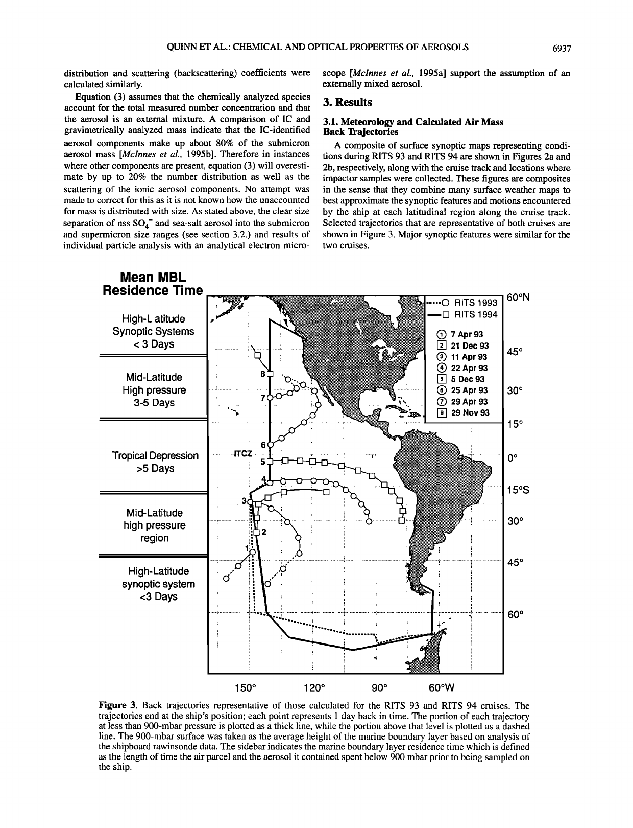
A composite of surface synoptic maps representing condi-

tions during RITS 93 and RITS 94 are shown in Figures 2a and

2b, respectively, along with the cruise track and locations where

impactor samples were collected. These figures are composites

in the sense that they combine many surface weather maps to

best approximate the synoptic features and motions encountered

by the ship at each latitudinal region along the cruise track.

Selected trajectories that are representative of both cruises are

shown in Figure 3. Major synoptic features were similar for the

two cruises.

Mean MBL

Residence Time

High-L atitude

Synoptic Systems

< 3 Days

Mid-Latitude

High pressure

3-5 Days

Tropical Depression

>5 Days

Mid-Latitude

high pressure

region

High-Latitude

synoptic system

<3 Days

: 8

• 6

..... IT. CZ ..........

: 5

ß .-0 RITS 1993

--i-i RITS 1994

(• 7 Apr 93

• 21 Dec 93

(•) 11 Apr93

• 22 Apr 93

• 5 Dec 93

(•) 25 Apr 93

(• 29 Apr 93

• 29 Nov 93

60øN

45 ø

30 ø

15 ø

15øS

30 ø

60 ø

150 ø 120 ø 90 ø 60øW

Figure 3. Back trajectories representative of those calculated for the RITS 93 and RITS 94 cruises. The

trajectories end at the ship's position; each point represents 1 day back in time. The portion of each trajectory

at less than 900-mbar pressure is plotted as a thick line, while the portion above that level is plotted as a dashed

line. The 900-mbar surface was taken as the average height of the marine boundary layer based on analysis of

the shipboard rawinsonde data. The sidebar indicates the marine boundary layer residence time which is defined

as the length of time the air parcel and the aerosol it contained spent below 900 mbar prior to being sampled on

the ship.

6938 QUINN ET AL.: CHEMICAL AND OPTICAL PROPERTIES OF AEROSOLS

At high latitudes (>45 o or 50ø), in both the northem and the

southern hemispheres, the passage of low-pressure systems from

west to east occurred every few days. Sea level pressures in

these regions were the lowest measured along both the RITS 93

and the RITS 94 cruise tracks. Subsidence of air from above the

marine boundary layer height of about 1000 m was associated

with frontal passages as indicated by trajectories (Figure 3,

trajectory 1) and increases in the ultrafine and Aitken particle

concentrations [Covert et al., 1995]. As a result, these regions

had short marine boundary layer residence times of about 1 day.

Here, the marine boundary layer residence time of an air parcel

and the aerosol it contains is defined as the length of time the

parcel spent below 900 mbar prior to being sampled on the ship.

This residence time was estimated from the calculated back

trajectories.

Belts of strong high-pressure systems moving from west to

east existed in the midlatitudes from about 40øS to 20øS and

from 20øN to 40øN. The latitudes given are approximate as the

position of these systems varied with season and year. The

location of the ship relative to the high-pressure systems

determined the trajectories of the air being sampled. During

RITS 93, as the ship traveled north from 50øS to 20øS, it

remained within one well-developed high. The transit of the ship

from the low-pressure region of the higher latitudes to this high-

pressure region in the midlatitudes is evidenced by the sharp

increase in sea level pressure from 960 to 1030 mbar (Figure

2a). On the equatorward side of the high, calculated trajectories

were from the southeast (Figure 3, trajectory 3). This air was

transported from the free troposphere at 55øS through the

southeast sector of the high. Subsidence followed by transport

along the edge of the high resulted in boundary layer residence

times of about 4 days. On the poleward side of the high, air

subsided from the free troposphere and was transported along

the southern edge of the high. Here, boundary layer residence

times were about 3 days.

During RITS 94, while traveling from north to south, the ship

entered the southern hemisphere midlatitudes as a low-pressure

system near Tahiti formed between two highs. The ship moved

with the low-pressure system from about 20øS to 40øS. Hence

there is only a gradual decrease in the measured sea level

pressure as the ship moved from 45øS to 60øS. Trajectories

(Figure 3, trajectory 2) indicate that the sampled air was

transported from the northeast along the surface to this low-

pressure region. The sampled air had a boundary layer residence

time of up to 5 days.

In the northern hemisphere midlatitudes during RITS 93 the

ship traveled through a pseudostationary high from about 20øN

to 40øN. On the equatorward side of the high the sampled air

was transported along the edge of the high from the northeast

with a boundary layer residence time of 3 to 5 days (Figure 3,

trajectory 7). High number and sulfate mass concentrations

indicate that this air had been continentally influenced prior to

its arrival at the ship. During RITS 94, as the ship moved from

north to south, a low-pressure system was encountered at 55øN

and again near 45øN. The ship traveled with the second low

until about 20 øN. Trajectories (Figure 3, trajectory 8) were of a

more marine origin than for RITS 93, with sampled air having

been transported from the northwest with a boundary layer

residence time of at least 2 days.

The well-developed midlatitude highs in both the northern

and the southern hemispheres led to a tropical depression

between about 20øS and 20øN. This low-pressure belt is

indicated by the decrease in measured sea level pressure for both

RITS 93 and RITS 94. Within this belt, air flowing around the

high-pressure systems resulted in relatively stable and consistent

marine boundary layer trade wind flow for both cruises. Easterly

trajectories (Figure 3, trajectories 4, 5, 6) indicated that the

sampled air masses had boundary layer residence times of up to

or more than 7 days. Based on atmospheric CO concentrations,

the Intertropical Convergence Zone (ITCZ) was located at about

2 øN during RITS 93 and between 5 o and 10øN during RITS 94

[Bates et al., 1995].

3.2. Size Distributions

Number- and chemical mass-size distributions were analyzed

for the regions described above as they each give information

about the aerosol. Modal features of the number distribution

reveal information about the age of the aerosol or degree to

which the aerosol has been affected by coagulation, condensa-

tion, and cloud processes [Covert et al., 1995]. Chemical mass

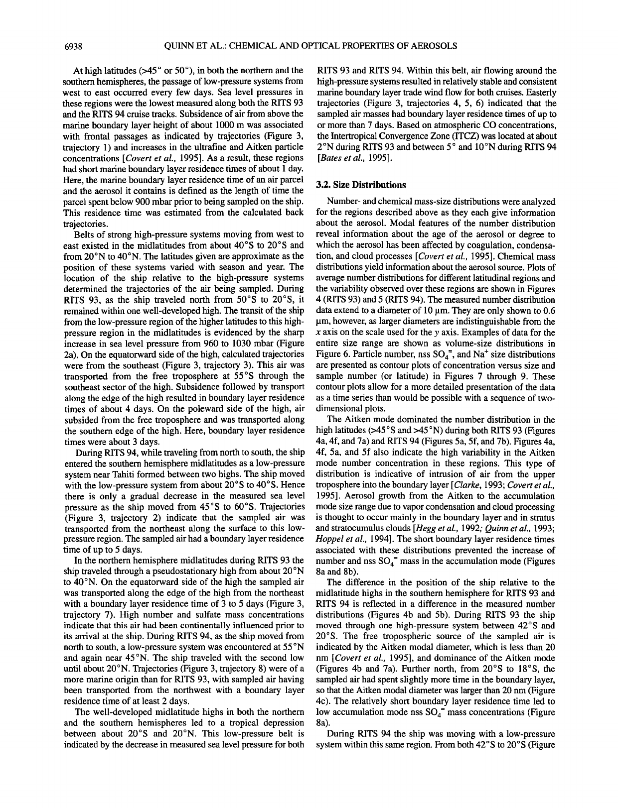
distributions yield information about the aerosol source. Plots of

average number distributions for different latitudinal regions and

the variability observed over these regions are shown in Figures

4 (RITS 93) and 5 (RITS 94). The measured number distribution

data extend to a diameter of 10 pm. They are only shown to 0.6

pm, however, as larger diameters are indistinguishable from the

x axis on the scale used for the y axis. Examples of data for the

entire size range are shown as volume-size distributions in

Figure 6. Particle number, nss SO4 =, and Na + size distributions

are presented as contour plots of concentration versus size and

sample number (or latitude) in Figures 7 through 9. These

contour plots allow for a more detailed presentation of the data

as a time series than would be possible with a sequence of two-

dimensional plots.

The Aitken mode dominated the number distribution in the

high latitudes (>45øS and >45 øN) during both RITS 93 (Figures

4a, 4f, and 7a) and RITS 94 (Figures 5a, 5f, and 7b). Figures 4a,

4f, 5a, and 5f also indicate the high variability in the Aitken

mode number concentration in these regions. This type of

distribution is indicative of intrusion of air from the upper

troposphere into the boundary layer [Clarke, 1993; Covert et al.,

1995]. Aerosol growth from the Aitken to the accumulation

mode size range due to vapor condensation and cloud processing

is thought to occur mainly in the boundary layer and in stratus

and stratocumulus clouds [Hegg et al., 1992; Quinn et al., 1993;

Hoppel et al., 1994]. The short boundary layer residence times

associated with these distributions prevented the increase of

number and nss SO4 = mass in the accumulation mode (Figures

8a and 8b).

The difference in the position of the ship relative to the

midlatitude highs in the southern hemisphere for RITS 93 and

RITS 94 is reflected in a difference in the measured number

distributions (Figures 4b and 5b). During RITS 93 the ship

moved through one high-pressure system between 42øS and

20øS. The free tropospheric source of the sampled air is

indicated by the Aitken modal diameter, which is less than 20

nm [Covert et al., 1995], and dominance of the Aitken mode

(Figures 4b and 7a). Further north, from 20øS to 18øS, the

sampled air had spent slightly more time in the boundary layer,

so that the Aitken modal diameter was larger than 20 nm (Figure

4c). The relatively short boundary layer residence time led to

low accumulation mode nss SO4 = mass concentrations (Figure

8a).

During RITS 94 the ship was moving with a low-pressure

system within this same region. From both 42øS to 20øS (Figure

QUINN ET AL.: CHEMICAL AND OPTICAL PROPERTIES OF AEROSOLS 6939

C: II

I I I I I I I I

0 0 0 0 0 0 0 0 0

0 0 0 0 0 0 0 0

I I I I I I I l

0 0 0 0 0 0 0 0 0

0 0 0 0 0 0 0 0

I I I I I I

II cn

•,• o

! I I I I I

0 0 0 0 0 0 0

0 0 0 0 0 0

I 1

0 0

=.wo 'dal•olPlNP

•:-wo 'dal•olPlNP

6940 QUINN ET AL.: CHEMICAL AND OPTICAL PROPERTIES OF AEROSOLS

II II

i i i i

o o o o

-q

II II •

I I I i

o o o o

1 i i i

o o o o

s- tuo 'da15olPlNP =- tuo 'da15olPlNP

QUINN ET AL.' CHEMICAL AND OPTICAL PROPERTIES OF AEROSOLS 6941

0.1

0.01

1E-3

1E-4

---o-- - R94 46S - 18S

-R94 15S- 5N

- R94 5N - 40N

........ R93 45S-19S

....... -R93 19S-10N

-R93 10N-40N

! i i i i i i , I ! ! ! , , ! , i I . i , , . , i . I

0.01 0 1 1 10

D, !.tin

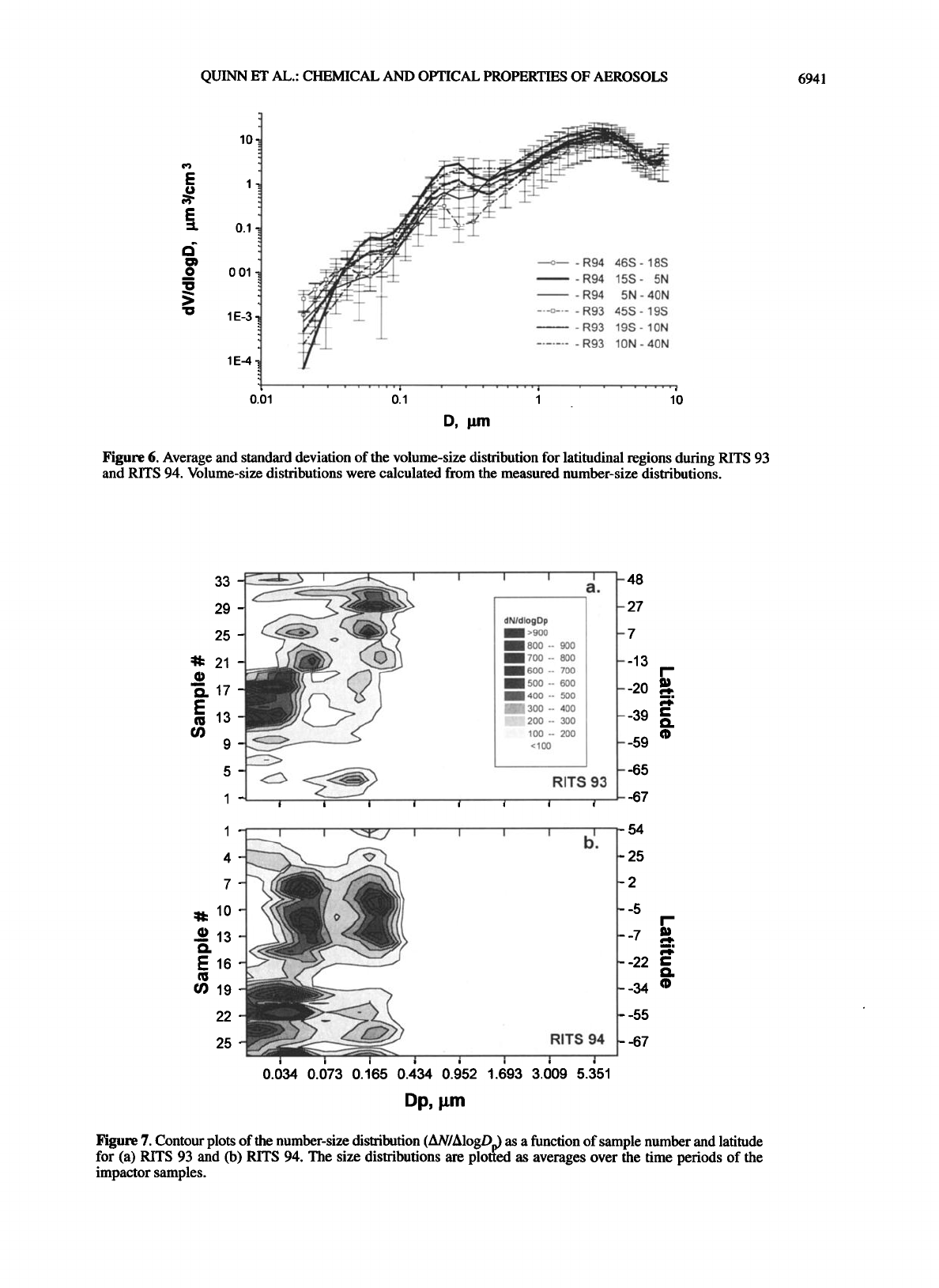
Figure 6. Average and standard deviation of the volume-size distribution for latitudinal regions during RITS 93

and RITS 94. Volume-size distributions were calculated from the measured number-size distributions.

• 21

•.17

• 13 .............. ..,.._,,...?•..i. 11 : .. :'. '

. - ---:---i-- .... ::::::::::::::::::::::::

........

1 I I I I

I I I I

i i

dNIdlogDp

• >900

1800 -- 900

1700 -- 800

1600 -- 700

1 500 -- 600

.__11•_ _ 400 -- 500

-"'"'":•'½•-.';•*..-4• 300 -- 400

100 -- 200

<100

RITS 93

i i

1 I I I I b !.

:1:1= 10

• 13

L'• i• .:?i i'•-i: !i•:.:..:. 5:.., :. "•i•!!::::•::.':'.'.•. :.:-: :: .• :"

• 19 :':-':':'""i.11 ..... "i'•:'•'.:•-.-:.?'::u.•: .....

25 RIIS 94

! I I I I I I I

0.034 0.073 0.165 0.434 0.952 1.693 3.009 5.351

Dp, gm

- 48

- 27

-7

--39 1=

I3.

- -59

- -65

- -67

- 54

-25

-2

--5

--22 1=

I3.

--34 •

- -55

- -67

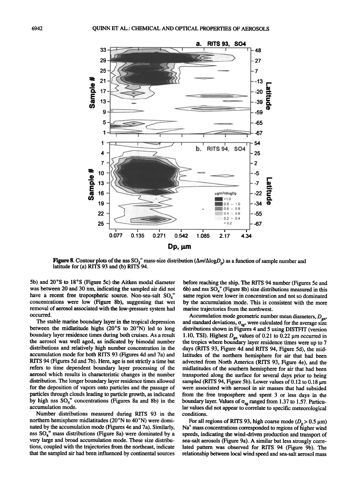
Figure 7. Contour plots of the number-size distribution (AN/AlogDp) as a function of sample number and latitude

for (a) RITS 93 and (b) RITS 94. The size distributions are plotted as averages over the time periods of the

impactor samples.

6942 QUINN ET AL.' CHEMICAL AND OPTICAL PROPERTIES OF AEROSOLS

a. RITS 93, SO4

33 -1.--4---•'""'"••'- ::'•••• ...................................... ""• "••••••"'.-•:'i...!• • • •

•!E?.--.:::-•.:...: :.,.,.,•: .......... •..:

, •:•.• •t.• • -•'.-

29 '• ........ ::

25 .... '?" '•'• .... ' ............ '

..•:::.. •:• ............ ;'.•. ,:.•:=•:" •

• •7

• ::. :?:. .••,.•.•:•.•...•.............:.:::.:::::::•,;::.:;•:•.-••

.............

m •3

9 •-.:.:...-.-......-. - :.-- .•

5 •/ •

! I

I I I

7 - ) .......... •' '" •"•• ........ •'•"'•"'"'•""•::•,,:,.:..

:g::: •,•. ß -r:•,,•:'•; ......

)..i• I

19 .............. •.....•.•.••.•..'...

I I I I

0.077 0.135 0.271 0.542

:#: 10-

•. 13-

• 16-

I I

1.085

I I

RITS 94, SO4

pglm$1dlogDp

• >1.0

._• 0.8 -- 1.0

.:•o.6 -- 0.8

•-71•:::;.!::•: 0.2 -- 0.4

< 0.2

2.17

• - 48

-27

-7

- -13

--20 _•,

--39

- -59

- -65

- -67

- 54

-25

-2

---5

--7

--22

--34

- -55

- -67

4.34

Dp, i•m

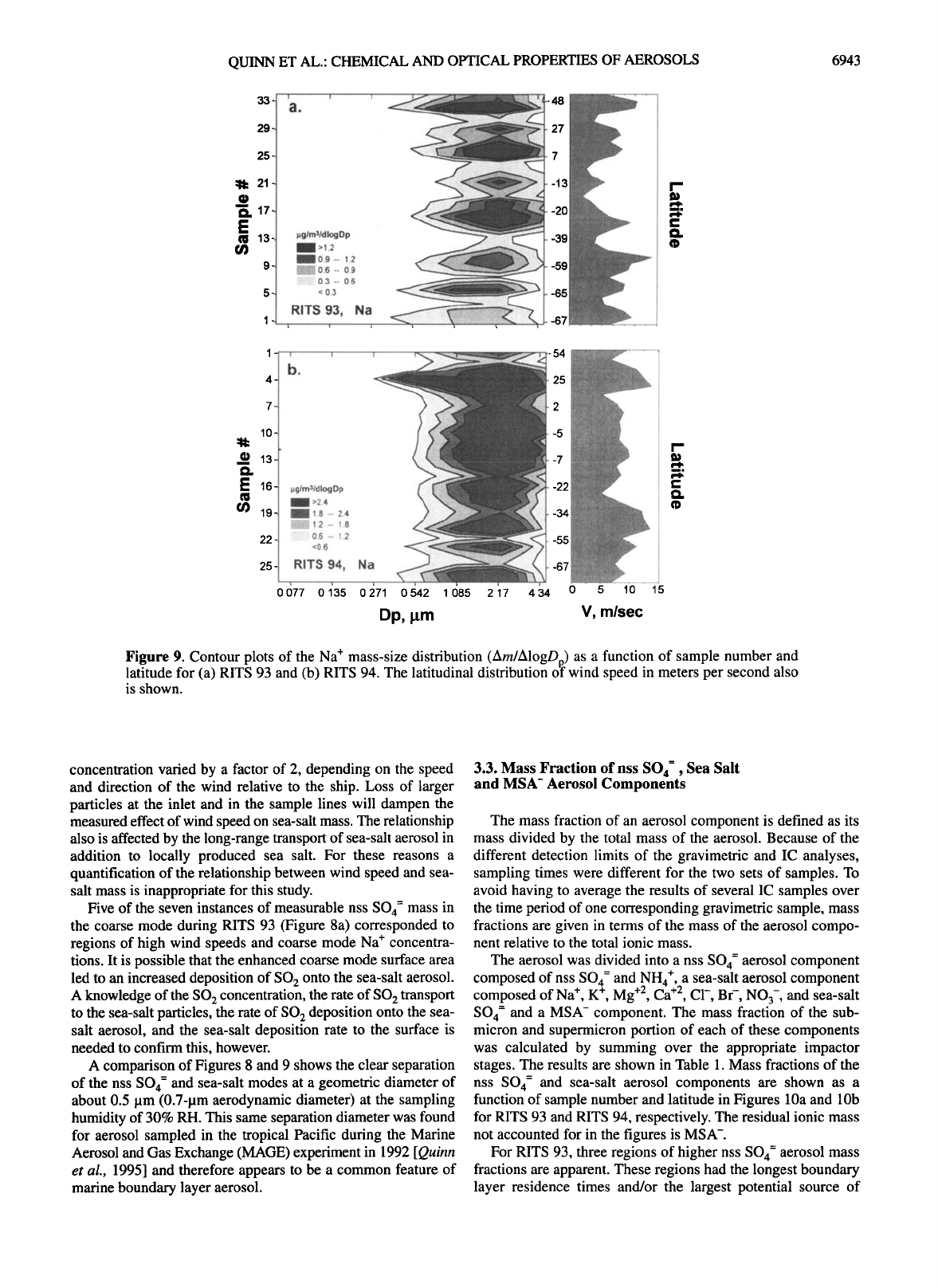
Figure 8. Contour plots of the nss SO4 = mass-size distribution (Am/AlogDp) as a function of sample number and

latitude for (a) RITS 93 and (b) RITS 94.

5b) and 20øS to 18øS (Figure 5c) the Aitken modal diameter

was between 20 and 30 nm, indicating the sampled air did not

have a recent free tropospheric source. Non-sea-salt SO 4-

concentrations were low (Figure 8b), suggesting that wet

removal of aerosol associated with the low-pressure system had

occurred.

The stable marine boundary layer in the tropical depression

between the midlatitude highs (20øS to 20øN) led to long

boundary layer residence times during both cruises. As a result

the aerosol was well aged, as indicated by bimodal number

distributions and relatively high number concentration in the

accumulation mode for both RITS 93 (Figures 4d and 7a) and

RITS 94 (Figures 5d and 7b). Here, age is not strictly a time but

refers to time dependent boundary layer processing of the

aerosol which results in characteristic changes in the number

distribution. The longer boundary layer residence times allowed

for the deposition of vapors onto particles and the passage of

particles through clouds leading to particle growth, as indicated

by high nss SO 4- concentrations (Figures 8a and 8b) in the

accumulation mode.

Number distributions measured during RITS 93 in the

northern hemisphere midlatitudes (20øN to 40øN) were domi-

nated by the accumulation mode (Figures 4e and 7a). Similarly,

nss SO 4- mass distributions (Figure 8a) were dominated by a

very large and broad accumulation mode. These size distribu-

tions, coupled with the trajectories from the northeast, indicate

that the sampled air had been influenced by continental sources

before reaching the ship. The RITS 94 number (Figures 5e and

6b) and nss SO 4- (Figure 8b) size distributions measured in this

same region were lower in concentration and not so dominated

by the accumulation mode. This is consistent with the more

marine trajectories from the northwest.

Accumulation mode geometric number mean diameters, D•n,

and standard deviations, o•, were calculated for the average size

distributions shown in Figures 4 and 5 using DISTFIT (version

1.10, TSI). Highest D•n values of 0.21 to 0.22 •m occurred in

the tropics where boundary layer residence times were up to 7

days (RITS 93, Figure 4d and RITS 94, Figure 5d), the mid-

latitudes of the northern hemisphere for air that had been

advected from North America (RITS 93, Figure 4e), and the

midlatitudes of the southern hemisphere for air that had been

transported along the surface for several days prior to being

sampled (RITS 94, Figure 5b). Lower values of 0.12 to 0.18 •m

were associated with aerosol in air masses that had subsided

from the free troposphere and spent 3 or less days in the

boundary layer. Values of o• ranged from 1.37 to 1.57. Particu-

lar values did not appear to correlate to specific meteorological

conditions.

For all regions of RITS 93, high coarse mode (Dp > 0.5 •m)

Na* mass concentrations corresponded to regions of higher wind

speeds, indicating the wind-driven production and transport of

sea-salt aerosols (Figure 9a). A similar but less strongly corre-

lated pattern was observed for RITS 94 (Figure 9b). The

relationship between local wind speed and sea-salt aerosol mass

QUINN ET AL.: CHEMICAL AND OPTICAL PROPERTIES OF AEROSOLS 6943

33-

29-

25-

•1• 21-

O. 17-

{• 13-

, I

p. glm31dlogDp

• >1.2

• 09 -- 1.2

•-- d-:•i ...... o.6 -- o.9

iiii•ii::!i!11iiii::ii.:: 0.3 -- 0.6

< 0.3

RITS 93, Na,

............... iiii•iii•:i,•,"" "-:: '"•

!i -39

¾•.:•i:• ......

- -155

- -67

__.• !3

• 16

03 19

i•gim31d log Dp

• >2.4

• 1.8 -- 2.4

....... '"';;'"'""-'-'"•d;i 1.2 -- 1.8

...........

::::::::::::::::::::: 0.6 1.2

:•'•:•'•:•:F': --

<0.6

RITS 94, Na

0.077 0.135 0.27!

Dp, pm

.•.• ß , ., ...,.•

%:' ..... '":,:•!:!iii!ii!i!;;--":":":•!i 2 ":•i'-,:' ..-

: -,..-..;-•..:..:.-, ....::::...:. , '--<:'

' ,:-::-•'--'-';..::::•:•':" '. -' ' i

: '.,"'i':'"'--'gi:% ...... •:?:.• -5

..... . :"-.':-"-'T'"'"":'"'""'" ':'•: .............

:-.;: .--;..i•:....-j•j;•ii?::•ii;i;::i•,:• ....... ;::;?.!.../....½•4;-: -22

..... ..........

0.542 1.085 2.!7 4.34 0 5 10

V, rnlsec

Figure 9. Contour plots of the Na + mass-size distribution (Am/AlogDp) as a function of sample number and

latitude for (a) RITS 93 and (b) RITS 94. The latitudinal distribution o'f wind speed in meters per second also

is shown.

concentration varied by a factor of 2, depending on the speed

and direction of the wind relative to the ship. Loss of larger

particles at the inlet and in the sample lines will dampen the

measured effect of wind speed on sea-salt mass. The relationship

also is affected by the long-range transport of sea-salt aerosol in

addition to locally produced sea salt. For these reasons a

quantification of the relationship between wind speed and sea-

salt mass is inappropriate for this study.

Five of the seven instances of measurable nss SO4 = mass in

the coarse mode during RITS 93 (Figure 8a) corresponded to

regions of high wind speeds and coarse mode Na + concentra-

tions. It is possible that the enhanced coarse mode surface area

led to an increased deposition of SO 2 onto the sea-salt aerosol.

A knowledge of the SO 2 concentration, the rate of SO 2 transport

to the sea-salt particles, the rate of SO 2 deposition onto the sea-

salt aerosol, and the sea-salt deposition rate to the surface is

needed to confirm this, however.

A comparison of Figures 8 and 9 shows the clear separation

of the nss SO4 = and sea-salt modes at a geometric diameter of

about 0.5 pm (0.7-pm aerodynamic diameter) at the sampling

humidity of 30% RH. This same separation diameter was found

for aerosol sampled in the tropical Pacific during the Marine

Aerosol and Gas Exchange (MAGE) experiment in 1992 [Quinn

et al., 1995] and therefore appears to be a common feature of

marine boundary layer aerosol.

3.3. Mass Fraction of nss SO4 = , Sea Salt

and MSA- Aerosol Components

The mass fraction of an aerosol component is defined as its

mass divided by the total mass of the aerosol. Because of the

different detection limits of the gravimetric and IC analyses,

sampling times were different for the two sets of samples. To

avoid having to average the results of several IC samples over

the time period of one corresponding gravimetric sample, mass

fractions are given in terms of the mass of the aerosol compo-

nent relative to the total ionic mass.

The aerosol was divided into a nss SO4 = aerosol component

composed of nss SO4 = and NH4 +, a sea-salt aerosol component

+2 +2

composed of Na +, K +, Mg , Ca , CI-, Br-, NO3- , and sea-salt

SO4 = and a MSA- component. The mass fraction of the sub-

micron and supermicron portion of each of these components

was calculated by summing over the appropriate impactor

stages. The results are shown in Table 1. Mass fractions of the

nss SO 4- and sea-salt aerosol components are shown as a

function of sample number and latitude in Figures 10a and 10b

for RITS 93 and RITS 94, respectively. The residual ionic mass

not accounted for in the figures is MS A-.

For RITS 93, three regions of higher nss SO4 = aerosol mass

fractions are apparent. These regions had the longest boundary

layer residence times and/or the largest potential source of

6944 QUINN ET AL.' CHEMICAL AND OPTICAL PROPERTIES OF AEROSOLS

Table 1. Percent Mass Fractions of Ionic Aerosol Components Relative to Measured Total or

Submicron Ionic Mass

RITS 93 RITS 94

Standard Standard

Component a Average Deviation Range Average Deviation Range

Percent Mass Fraction of Total Measured Ionic Mass

Super-gm sea salt 81 9 58-93 82 5.8 69-92

Sub-tam sea salt 10 7 1.4-28 8.3 4.6 2.7-19

Sub-tam nss SO4 = 7 8.3 0.2-34 6 3.7 0.9-13

Super-tam nss SO4 = 1.3 1 0.2-3.8 0.8 1 0.1-5.5

Sub-tam MSA- 0.39 0.48 0.08-2.7 1.0 1.6 0.03-6.0

Super-tam MSA- 0.24 0.37 0.03-2.0 0.40 0.29 0.03-1.1

Percent Mass Fraction of Submicron Measured Ionic Mass

Sub-tam sea salt 55 79 10-98 54 22 21-91

Sub-tam nss SO4 = 36 28 2-90 39 23 6-76

Sub-pm MSA- 2.1 1.7 0.31-10 5.5 6.6 0.37-24

Percent mass fractions are defined as the mass of the aerosol component divided by the measured

ionic mass.

aThe nss SO4 = aerosol component includes the associated NH4 + mass. The sea-salt aerosol

component includes Na +, K +, Mg +2, Ca +2, CI-, Br-, NO3-, and sea-salt SO4 =.

sulfate aerosol. From 27øN to 38øN where, according to number

and nss SO4 = concentrations, continentally influenced aerosol

had been advected in a nonprecipitating air mass from North

America, the mass fraction of nss SO4 = aerosol was the highest

measured, ranging from 23 to 37%. In the tropics, between 19 øS

and 2 øN, where boundary layer residence times were the longest

I• su•mSS •..•.•.*: ........... :::.•::::::.•::::::::.'.: ..................................... :" ............ • .................. =='

10 t• supumSS ................................... '•"• ............................................................... ß :':.-'•. -5

1•1 ...... ,,..x•x,•..•....,.,, .....: ........... ,..... ,...,,...., ..•... ::::::::::::::::::::::::::::::::::::::::::::::::::::::::::::::::::::::::::::::::::::::::::::::::::::::::::::::::::::::::::::::: 1

• :::::::::::::::::::::::::::::::::::::::::::::::::::::::::::::::::::::::::::::::::::::::::::::::::::::::::::::::::::::::::::::::::::::::::::::::::::::::::::::::::::::::::::: •

::::::::::::::::::::::::::::::::::::::::::::::::::::::::::::::::::::::::::::::::::::::::::::::::::::::::::::::::::::::::::::::::::::::::::::::::::::::::::::::::::::::::::::::::::::::::::::::::::::::::::::::::::::::::::::::::::: •

:::::::::::::::::::::::::::::::::::::::::::::::::::::::::::::::::::::::::::::::::::::::::::::::::::::::::::::::::::::::::::::::::::::::::::::::::::::::::::::::::::::::::::::::::::::::::::: 1

..,:.:::.:: =========================================================================================================================== ......

: :. :::•i:•:i:•:::•.}:•:•:•:..`•:•:•:g•:•:::::::.`.5.`.•:•.`.[•<:•:..`.i:.•..•:•:[:•:E:5:•:•:::5:[:•:[•:i•:[:{:;•:•:•:•:•:•:;•:•:s::•::` •l -67

0 20 40 60 80 100

Percent of total ionic mass

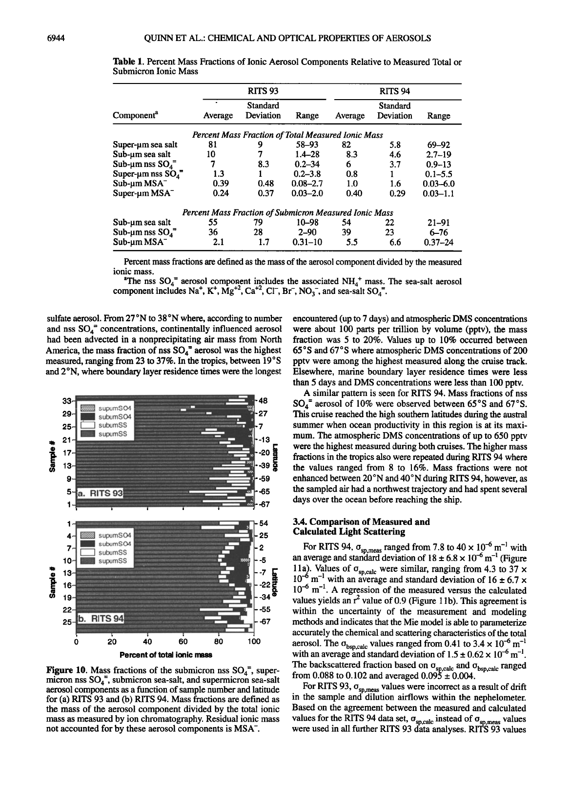
Figure 10. Mass fractions of the submicron nss SO4 =, super-

micron nss SO4 =, submicron sea-salt, and supermicron sea-salt

aerosol components as a function of sample number and latitude

for (a) RITS 93 and (b) RITS 94. Mass fractions are defined as

the mass of the aerosol component divided by the total ionic

mass as measured by ion chromatography. Residual ionic mass

not accounted for by these aerosol components is MSA-.

encountered (up to 7 days) and atmospheric DMS concentrations

were about 100 parts per trillion by volume (pptv), the mass

fraction was 5 to 20%. Values up to 10% occurred between

65øS and 67øS where atmospheric DMS concentrations of 200

pptv were among the highest measured along the cruise track.

Elsewhere, marine boundary layer residence times were less

than 5 days and DMS concentrations were less than 100 pptv.

A similar pattern is seen for RITS 94. Mass fractions of nss

SO4 = aerosol of 10% were observed between 65øS and 67øS.

This cruise reached the high southern latitudes during the austral

summer when ocean productivity in this region is at its maxi-

mum. The atmospheric DMS concentrations of up to 650 pptv

were the highest measured during both cruises. The higher mass

fractions in the tropics also were repeated during RITS 94 where

the values ranged from 8 to 16%. Mass fractions were not

enhanced between 20øN and 40øN during RITS 94, however, as

the sampled air had a northwest trajectory and had spent several

days over the ocean before reaching the ship.

3.4. Comparison of Measured and

Calculated Light Scattering

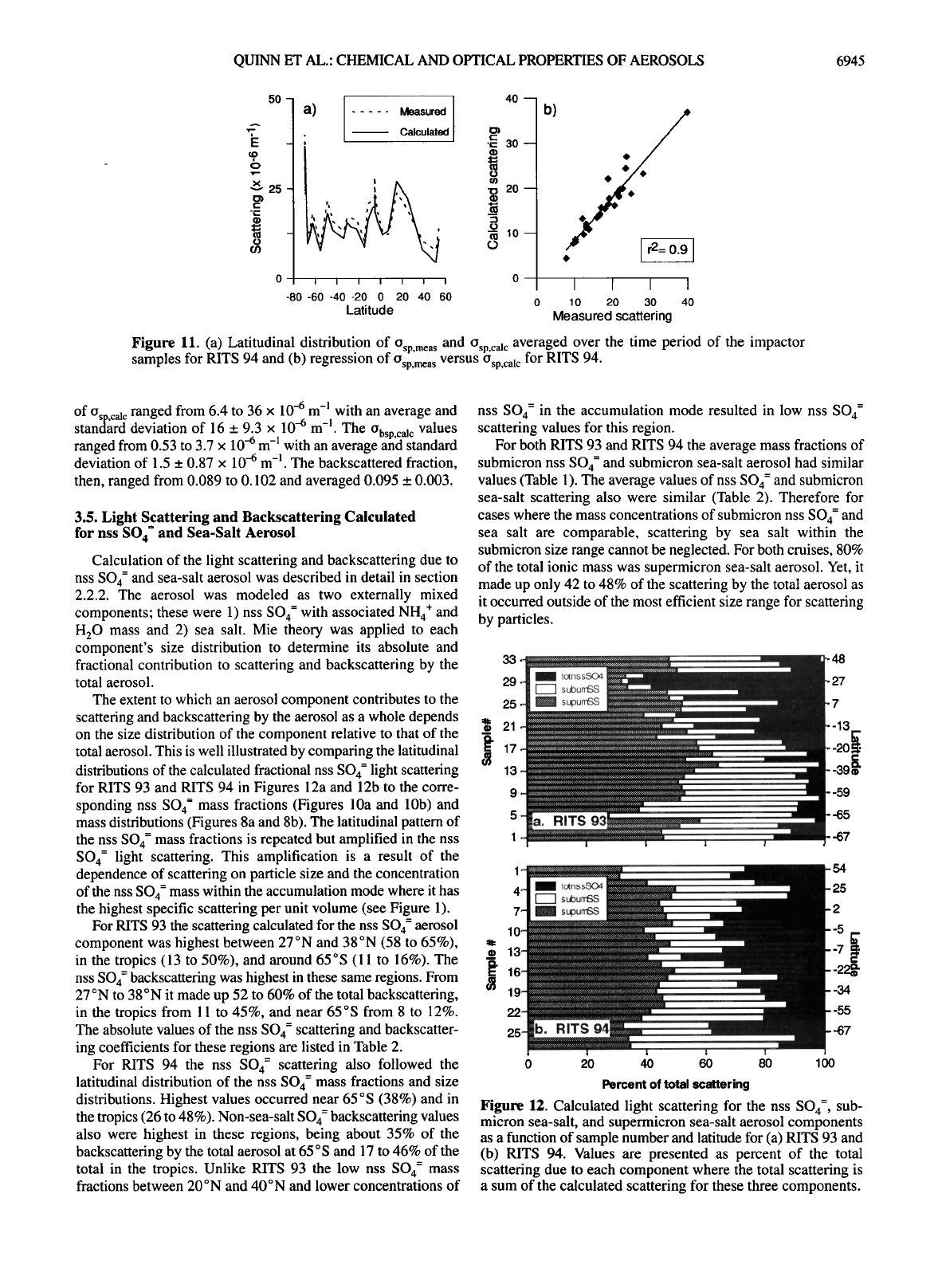
For RITS 94, (Jsp,meas ranged from 7.8 to 40 x 10 -6 m -1 with

an average and standard deviation of 18 + 6.8 x 10-6 m -1 (Figure

1 la). Values of O•p,c• c were similar, ranging from 4.3 to 37 x

10-6 m -I with an average and standard deviation of 16 _+ 6.7 x

10-6 m -1. A regression of the measured versus the calculated

values yields an r 2 value of 0.9 (Figure 11 b). This agreement is

within the uncertainty of the measurement and modeling

methods and indicates that the Mie model is able to parameterize

accurately the chemical and scattering characteristics of the total

aerosol. The Obsp,calc values ranged from 0.41 to 3.4 x 10-6 m -1

with an average and standard deviation of 1.5 + 0.62 x 10-6 m -].

The backscattered fraction based on O sp,cal c and Obsp,calc ranged

from 0.088 to 0.102 and averaged 0.095 + 0.004.

For RITS 93, Osp,mea s values were incorrect as a result of drift

in the sample and dilution airflows within the nephelometer.

Based on the agreement between the measured and calculated

values for the RITS 94 data set, o,p c•c instead of o,p meas values

were used in all further RITS 93 d•ta analyses. RIT• 93 values

QUINN ET AL.: CHEMICAL AND OPTICAL PROPERTIES OF AEROSOLS 6945

50-

•x 25-

-• _

..... Measured

Calculated

I I I I I I I

-80-60-40-20 0 20 40 60

Latitude

40--

• 10--

0 10 20 30 40

Measured scattering

Figure 11. (a) Latitudinal distribution of Osp,mea s and Osp,cal c averaged over the time period of the impactor

samples for RITS 94 and (b) regression of Osp,mea s versus Osp,cal c for RITS 94.

of Osp,cal c ranged from 6.4 to 36 x 10 -6 m -• with an average and

standard deviation of 16 _+ 9.3 x 10 -6 m -]. The Obsp,calc values

ranged from 0.53 to 3.7 x 10 -6 m -! with an average and standard

deviation of 1.5 _+ 0.87 x 10 -6 m -]. The backscattered fraction,

then, ranged from 0.089 to 0.102 and averaged 0.095 _+ 0.003.

3.5. Light Scattering and Backscattering Calculated

for nss SO4 = and Sea-Salt Aerosol

Calculation of the light scattering and backscattering due to

nss SO4 = and sea-salt aerosol was described in detail in section

2.2.2. The aerosol was modeled as two externally mixed

components; these were 1) nss SO4 = with associated NH4 + and

H20 mass and 2) sea salt. Mie theory was applied to each

component's size distribution to determine its absolute and

fractional contribution to scattering and backscattering by the

total aerosol.

The extent to which an aerosol component contributes to the

scattering and backscattering by the aerosol as a whole depends

on the size distribution of the component relative to that of the

total aerosol. This is well illustrated by comparing the latitudinal

distributions of the calculated fractional riss SO4 = light scattering

for RITS 93 and RITS 94 in Figures 12a and 12b to the corre-

sponding nss SO4 = mass fractions (Figures 10a and 10b) and

mass distributions (Figures 8a and 8b). The latitudinal pattern of

the nss SO4 = mass fractions is repeated but amplified in the nss

SO4 = light scattering. This amplification is a result of the

dependence of scattering on particle size and the concentration

of the nss SO4 = mass within the accumulation mode where it has

the highest specific scattering per unit volume (see Figure 1).

For RITS 93 the scattering calculated for the nss SO4 = aerosol

component was highest between 27øN and 38øN (58 to 65%),

in the tropics (13 to 50%), and around 65øS (11 to 16%). The

nss SO4 = backscattering was highest in these same regions. From

27øN to 38øN it made up 52 to 60% of the total backscattering,

in the tropics from 11 to 45%, and near 65øS from 8 to 12%.

The absolute values of the nss SO4 = scattering and backscatter-

ing coefficients for these regions are listed in Table 2.

For RITS 94 the nss SO4 = scattering also followed the

latitudinal distribution of the nss SO4 = mass fractions and size

distributions. Highest values occurred near 65øS (38%) and in

the tropics (26 to 48%). Non-sea-salt SO4 = backscattering values

also were highest in these regions, being about 35% of the

backscattering by the total aerosol at 65øS and 17 to 46% of the

total in the tropics. Unlike RITS 93 the low nss SO4 = mass

fractions between 20 øN and 40øN and lower concentrations of

nss SO4 = in the accumulation mode resulted in low nss SO4 =

scattering values for this region.

For both RITS 93 and RITS 94 the average mass fractions of

submicron nss SO4 = and submicron sea-salt aerosol had similar

values (Table 1 ). The average values of nss SO4 = and submicron

sea-salt scattering also were similar (Table 2). Therefore for

cases where the mass concentrations of submicron nss SO4 = and

sea salt are comparable, scattering by sea salt within the

submicron size range cannot be neglected. For both cruises, 80%

of the total ionic mass was supermicron sea-salt aerosol. Yet, it

made up only 42 to 48% of the scattering by the total aerosol as

it occurred outside of the most efficient size range for scattering

by particles.

33 .<- ...... ß ............................. • ......................................... ,, .... . 48

:.::.::.:..•:.:...:.:....:..,:..,.•xxxx,-,,.,,.,,,vx• i

29 ß • t•nss•

......... 27

:: • s•u• ............

25 : • s•u• ................................ 7

• 21 ........................................................................... 13

• ...... :::::::::::::::::::::::::::::::::::::::::::::::::::::::::::::::: ............................

17 .......................... ;•:•.•.•2•7•`;}•<:::•7``;;7•`•7•;•>•.•``:`2•``•;:`•J<•::•.•;•:;•`;•2•` -20 •.

9 •``•``*•``•.`*•```•``•`•```•<<*•``•.•`•.•>•:•.. -59

:::::::::::::::::::::::::::::::::::::::::::::::::::::::::::::::::::::::::::::::::::::::::::::::::::::::::::

:+xx.x•,x,x,:.:.xx.xx.:.:.x.>x,•x,x.:.:.x.:.>>:.:.x.x+x,x.x,x.:,,:..

•>>:.>:.:.:.:.•.:.:.:.:.>x.•.>>•.:.•.•.:.>m.:•:.:.:.•.:.•.•.:.•.•.:•>x`•:.:.x.•.•.:.:.x.:..

5 •a. RITS 93 ................................................................................... -65

.x.>:.x.:•,x.x<<,x•<,,x.:.:•<<.:.:..,:.:<,,:.x.:.x<•,xx+•,x•xx,>x•,x•x,:,xq

1 ............................................................................................................. •7

4 I totnssSO4 ::::::::::::::::::::::::::::

:•:•:..,.?/.,..:•,<:•:•:•:?/::.x;:..,.•:•$?/:•:

ß 1= ::::: .•:::•::•:: ,x3 •:: •:•: :: :.<:•:: •<::: •:::: :: :s:::::: •::.,..!: :: 3: ::::::::::::::::::::::::: :::::: •::::: :: s :::• .,.:: :::::::.:.

(j• :!:.•:`.``3x.`.•3:i:•3.``3•.``.:•:•!.`..`q•:!:•3::•:..`.::•:•:.•:•:•:;:•.x.•:3:•:•:.:..•:35:•:3•!8?.`..•:!:.``i•:!:•:3•

:::::...:.:.:.:.:.:.:.:.:.:.:.:.:.:.:.:.-...:.:.....: x... =================================================

25 ::i:::b. RITS 94

:•::...•.:.:.:`:.:.:.x•.:.:.:.:.`•:.`.•.:.:.:.:...:.:.•...:.•.:.•...•.:.:+:.:•::::::::.•:::::•

:::::::::::::::::::::::::::::::::::::::::::::::::::::::::::::::::::::::::::::::::::::::::::

0 20 40 60 80 lOO

-5 g.

-7 •.

-22•

-34

-55

-67

Percent of total scattering

Figure 12. Calculated light scattering for the nss SO4 =, sub-

micron sea-salt, and supermicron sea-salt aerosol components

as a function of sample number and latitude for (a) RITS 93 and

(b) RITS 94. Values are presented as percent of the total

scattering due to each component where the total scattering is

a sum of the calculated scattering for these three components.

6946 QUINN ET AL.' CHEMICAL AND OPTICAL PROPERTIES OF AEROSOLS

Table 2. Scattering and Backscattering Coefficients Calculated for nss SO4 =, Submicron Sea

Salt, and Supermicron Sea-Salt Aerosol Components for Latitudinal Regions Where nss SO 4-

Had the Largest Contribution to Scattering by Total Aerosol

NH Midlatitudes Tropics

27øN to 38øN 20øS to 20øN

Coefficient,

x 10 -6 m -1 RITS 93 RITS 94 RITS 93 RITS 94 RITS 93 RITS 94

S H Hi gh Latitudes

65 øS to 67øS

11-18 1.8-2.4 1.4-9.4 2.9-9.3 1.3-2.1 1.7-5.6

IJsp,SO4,aer

Osp,sub,seasalt 0.43-2.5 2.9-8.6 0.72-11 1.8-11 2.5-13 2.3-18

Osp,sup,seasalt 5.2-10 3.2-11 2.6-19 3.8-13 2.3-6.7 3.7-13

Obsp,SO4,ae r 0.89--1.4 0.12-0.16 0.12--0.62 0.22-0.83 0.1-0.13 0.33--0.39

Obsp,sub,seasal t 0.1-0.23 0.23-0.71 0.10-0.95 0.16-0.85 0.21-1.0 0.19-1.5

Obsp,sup,seasal t 0.57-1.1 0.35-1.2 0.28-2.1 0.41-1.5 0.27-1.1 0.41-1.5

NH, northern hemisphere; SH, southern hemisphere.

3.6. Mass Scattering Efficiencies for the nss SO4--

and Sea-Salt Aerosol Components

Mass scattering efficiencies for individual aerosol com-

ponents can be estimated from a multiple linear regression of the

mass concentration of each aerosol component against the

scattering coefficient for the whole aerosol. For the RITS 93 and

RITS 94 data sets a regression of the following form, including

only the major aerosol components, was used to obtain weighted

averages of the scattering efficiencies

: {z tn

(Jsp,calc {Zsp,SO4,ion mso4,ion + sp,sub,seasalt sub,seasalt

+ sp,sup,seasalt sup,seasalt

•z m

(4)

The mass scattering efficiency of nss SO4 = ({Zsp,SO4,ion) is given

in terms of the unit mass of nss SO 4- ion as it is the ion concen-

tration or column burden that is predicted by chemical transport

models [e.g., Langner and Rodhe, 1991]. Values of mso4,ion

include both the submicron and supermicron size fractions since

the majority of the nss SO 4- mass (>75%) occurred in the

submicron size range and this is the size range expected to have

the most significant effect on scattering by the total aerosol.

Unlike the nss SO4 = aerosol component, the majority of the

sea-salt aerosol mass was in the supermicron size fraction which

will not have a large influence on scattering by the total aerosol

unless it overwhelms the total particle mass concentration. To

consider the more relevant submicron fraction, the sea-salt

component was divided into submicron and supermicron size

ranges resulting in a submicron mass scattering efficiency

({gsp,sub,seasalt) and a supermicron mass scattering efficiency

({gsp,sup,seasalt). Mass backscattering efficiencies for the aerosol

components were calculated by substituting the calculated

backscattering coefficient, IJbsp,calc, for the whole aerosol into

(4).

The calculated mass scattering and backscattering efficiencies

averaged over latitudinal regions of the Pacific from RITS 93

and RITS 94 are shown in Table 3. For RITS 93 the weighted

average and standard error from the regression of {gsp,SO4,ion for

all samples were 5.1 + 0.21 m 2 g-• and for RITS 94, 3.8 + 0.35

m 2 g-•. Values were relatively constant over all latitudinal

regions with weighted averages ranging from 4.3 to 7.5 m 2 g-•.

The stability of the values is a reflection of the narrow range of

Dg n and Osg measured throughout both cruises (see Table 4).

More variability in {gsp,SO4,ion is expected in instances where Dg n

and Osg for the nss SO4 = aerosol component vary in space or

time (see, for example, Zhang et al. [1994]). The largest values

were observed in the northern hemisphere high latitudes (40 øN

to 55 øN) and in marine air masses in the southern and northern

hemisphere midlatitudes (40øS to 20øS and 20øN to 40øN).

Lowest values were found in the tropics between 20øS and

20øN.

The average and standard deviation of {gbsp,SO4,ion was about

an order of magnitude lower and displayed less variability than

the scattering efficiency values. The weighted average and

standard error of all RITS 93 samples were 0.43 + 0.02 m 2 g-•

and for RITS 94, 0.40 + 0.03 m 2 g-•. Weighted averages ranged

from 0.41 to 0.58 m 2 g-• over all latitudinal regions. The lower

degree of variability in the backscattering efficiencies compared

to the scattering efficiencies is a result of a weaker dependence

of Obs p than Osp on particle size for diameters between 0.2 and

1.0 pm [Marshall, 1994].

The weighted average and standard error of {gsp,sub,seasalt for

RITS 93 were 5.0 + 0.27 m 2 g-• and for RITS 94, 4.9 +

0.24 m 2 g-•. Values of {gbsp,sub,seasal t for RITS 93 averaged 0.47

2 1

_+ 0.03 m g- and for RITS 94 averaged 0.42 _+ 0.02 m 2 g-•.

The equivalent values for {gsp,SO4,ion and {gsp,sub,seasalt as well as

{gbsp,SO4,ion and {gbsp,sub,seasal t indicate that if the submicron masses

of sea salt and nss SO4 = are comparable, the contribution by

submicron sea salt to scattering and backscattering by the

aerosol as a whole cannot be neglected given that the submicron

sea salt and nss SO4 = aerosol have similar lifetimes in the

atmosphere.

Mass scattering and backscattering efficiencies for the

supermicron sea-salt component were appreciably lower,

however, as it is in a size range where particle scattering in the

visible is less efficient per unit volume. RITS 93 and RITS 94

2 1

values of {ZSlP,SUp,seasal t averaged 0.88 _+ 0.05 m g- and 0.92 _+

0.07 m 2 g-, respectively. RITS 93 and RITS 94 values of

{gbsp,sup,seasal t averaged 0.08 + 0.01 m 2 g-• and 0.09 + 0.01 m 2

respectively. The lack of variability in the scattering and

backscattering efficiencies of the sea-salt aerosol suggests that

QUINN ET AL.: CHEMICAL AND OPTICAL PROPERTIES OF AEROSOLS 6947

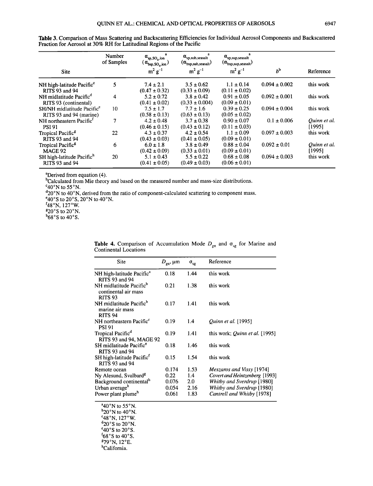
Table 3. Comparison of Mass Scattering and Backscattering Efficiencies for Individual Aerosol Components and Backscattered

Fraction for Aerosol at 30% RH for Latitudinal Regions of the Pacific

Number i•sp,so4,ion a i•sp,sub,seasalt a i•sp,sup,seasalt a

of Samples ( {gbsp,SO4,io n ) ({gbsp,sub,seasalt) ({gbsp,sup,seasalt)

Site m 2 g-• m 2 g-• m 2 g-• b b Reference

NH high-latitude Pacific c 5 7.4 _+ 2.1 3.5 _+ 0.62 1.1 _+ 0.14 0.094 _+ 0.002 this work

RITS 93 and 94 (0.47 _+ 0.32) (0.33 _+ 0.09) (0.11 _+ 0.02)

NH midlatitude Pacific d 4 5.2 _+ 0.72 3.8 _+ 0.42 0.91 _+ 0.05 0.092 _+ 0.001 this work

RITS 93 (continental) (0.41 + 0.02) (0.33 + 0.004) (0.09 + 0.01)

SH/NH midlatitude Pacific e 10 7.5 + 1.7 7.7 + 1.6 0.39 + 0.25 0.094 +_ 0.004 this work

RITS 93 and 94 (marine) (0.58 _+ 0.13) (0.63 _+ 0.13) (0.05 _+ 0.02)

NH northeastern Pacific f 7 4.2 + 0.48 3.7 + 0.38 0.90 + 0.07 0.1 + 0.006 Quinn et al.

PSI91 (0.46_+0.15) (0.43_+0.12) (0.11 _+0.03) [1995]

Tropical Pacific g 22 4.3 _+ 0.37 4.2 _+ 0.54 1.1 +_ 0.09 0.097 _+ 0.003 this work

RITS 93 and 94 (0.43 _+ 0.03) (0.41 _+ 0.05) (0.09 _+ 0.01)

Tropical Pacific g 6 6.0 _+ 1.8 3.8 _+ 0.49 0.88 _+ 0.04 0.092 _+ 0.01 Quinn et al.

MAGE 92 (0.42 _+ 0.09) (0.33 _+ 0.01) (0.09 _+ 0.01) [ 1995]

SH high-latitude Pacific h 20 5.1 _+ 0.43 5.5 _+ 0.22 0.68 _+ 0.08 0.094 _+ 0.003 this work

RITS 93 and 94 (0.41 _+ 0.05) (0.49 _+ 0.03) (0.06 _+ 0.01)

aDerived from equation (4).

bCalculated from Mie theory and based on the measured number and mass-size distributions.

c40øN to 55øN.

d20øN to 40øN, derived from the ratio of component-calculated scattering to component mass.

e40øS to 20øS, 20øN to 40øN.

f48øN, 127øW.

g20øS to 20øN.

h68 o S to 40 ø S.

Table 4. Comparison of Accumulation Mode Dg n and Osg for Marine and

Continental Locations

Site Dgn, t am (Jsg Reference

NH high-latitude Pacific a 0.18 1.44

RITS 93 and 94

NH midlatitude Pacific b 0.21 1.38

continental air mass

RITS 93

NH midlatitude Pacificb 0.17 1.41

marine air mass

RITS 94

NH northeastern Pacific c 0.19 1.4

PSI 91

Tropical Pacific d 0.19 1.41

RITS 93 and 94, MAGE 92

SH midlatitude Pacific e 0.18 1.46

RITS 93 and 94

SH high-latitude Pacific f 0.15 1.54

RITS 93 and 94

Remote ocean 0.174 1.53

Ny Alesund, Svalbard g 0.22 1.4

Background continental h 0.076 2.0

Urban average h 0.054 2.16

Power plant plume h 0.061 1.83

this work

Quinn et al. [1995]

this work; Quinn et al. [1995]

this work

Meszaros and Vissy [1974]

Covert and Heintzenberg [ 1993]

Whitby and Sverdrup [ 1980]

Canttell and Whitby [1978]

a40øN to 55øN.

b20øN tO 40øN.

c48 øN, 127 øW.

d20øS tO 20øN.

%0 o S to 20 ø S.

f68 o S to 40 ø S.

g79 øN, 12øE.

hCalifornia.

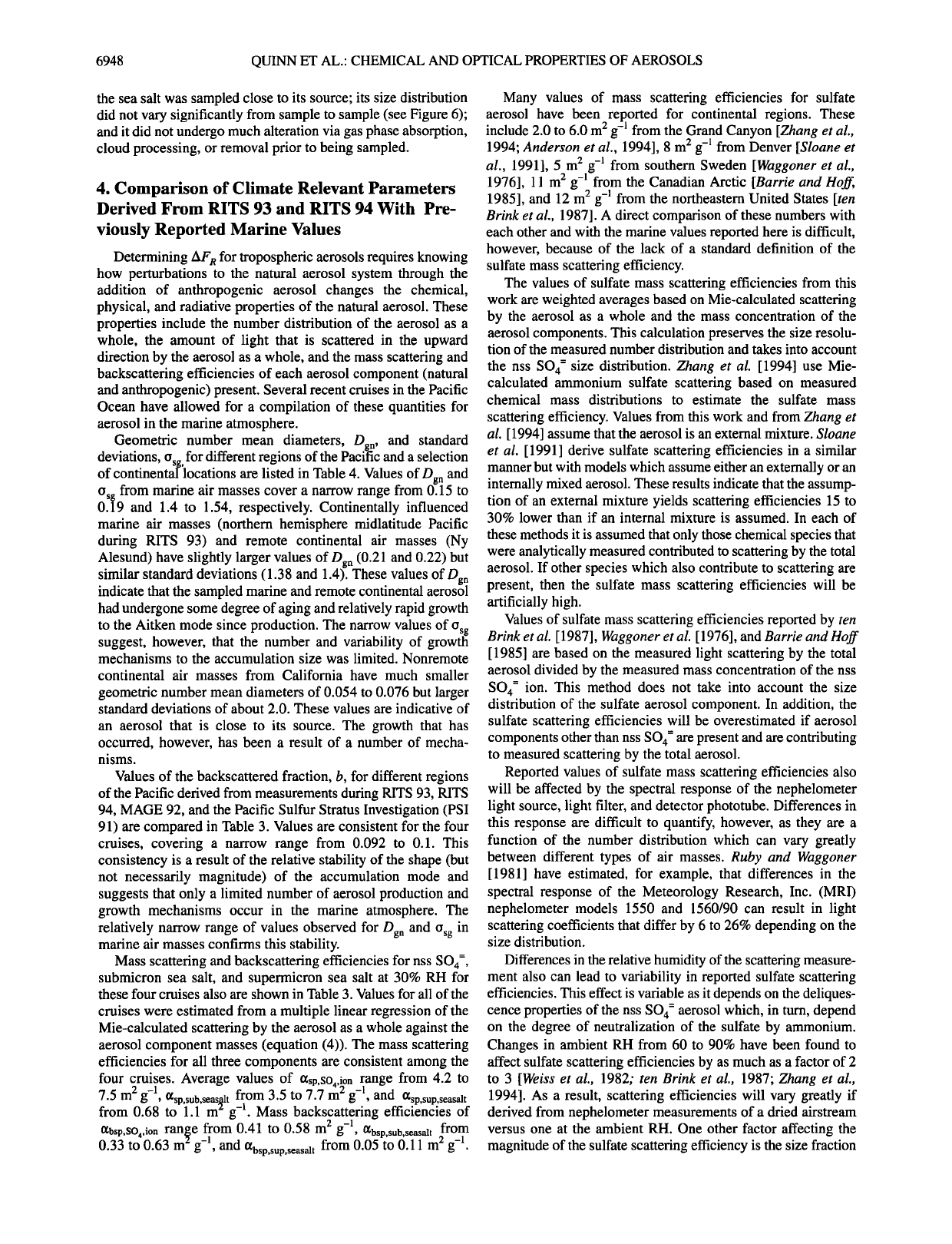
6948 QUINN ET AL.: CHEMICAL AND OPTICAL PROPERTIES OF AEROSOLS

the sea salt was sampled close to its source; its size distribution

did not vary significantly from sample to sample (see Figure 6);

and it did not undergo much alteration via gas phase absorption,

cloud processing, or removal prior to being sampled.

4. Comparison of Climate Relevant Parameters

Derived From RITS 93 and RITS 94 With Pre-

viously Reported Marine Values

Determining AF• for tropospheric aerosols requires knowing

how perturbations to the natural aerosol system through the

addition of anthropogenic aerosol changes the chemical,

physical, and radiative properties of the natural aerosol. These

properties include the number distribution of the aerosol as a

whole, the amount of light that is scattered in the upward

direction by the aerosol as a whole, and the mass scattering and

backscattering efficiencies of each aerosol component (natural

and anthropogenic) present. Several recent cruises in the Pacific

Ocean have allowed for a compilation of these quantities for

aerosol in the marine atmosphere.

Geometric number mean diameters, Dgn, and standard

deviations, Osg ' for different regions of the Pacific and a selection

of continental locations are listed in Table 4. Values of Dg n and

Osg from marine air masses cover a narrow range from 0.15 to

0.19 and 1.4 to 1.54, respectively. Continentally influenced

marine air masses (northern hemisphere midlatitude Pacific

during RITS 93) and remote continental air masses (Ny

Alesund) have slightly larger values of Dg n (0.21 and 0.22) but

similar standard deviations (1.38 and 1.4). These values of Dg n

indicate that the sampled marine and remote continental aerosol

had undergone some degree of aging and relatively rapid growth

to the Aitken mode since production. The narrow values of Osg

suggest, however, that the number and variability of growth

mechanisms to the accumulation size was limited. Nonremote

continental air masses from California have much smaller

geometric number mean diameters of 0.054 to 0.076 but larger

standard deviations of about 2.0. These values are indicative of

an aerosol that is close to its source. The growth that has

occurred, however, has been a result of a number of mecha-

nisms.

Values of the backscattered fraction, b, for different regions

of the Pacific derived from measurements during RITS 93, RITS

94, MAGE 92, and the Pacific Sulfur Stratus Investigation (PSI

91) are compared in Table 3. Values are consistent for the four

cruises, coveting a narrow range from 0.092 to 0.1. This

consistency is a result of the relative stability of the shape (but

not necessarily magnitude) of the accumulation mode and

suggests that only a limited number of aerosol production and

growth mechanisms occur in the marine atmosphere. The

relatively narrow range of values observed for Dg n and Osg in

marine air masses confirms this stability.

Mass scattering and backscattering efficiencies for nss SO4 =,

submicron sea salt, and supermicron sea salt at 30% RH for

these four cruises also are shown in Table 3. Values for all of the

cruises were estimated from a multiple linear regression of the

Mie-calculated scattering by the aerosol as a whole against the

aerosol component masses (equation (4)). The mass scattering

efficiencies for all three components are consistent among the

four cruises. Average values of ttsp,S% ion range from 4.2 to

2 -1 "2 -1

7.5 m g , •sp,sub,seas•lt fr•om 3.5 to 7.7 m g , and •sp,sup, seasalt

from 0.68 to 1.1 m g-'. Mass backscattering efficiencies of

{gbsp,SO4,ion range from 0.41 to 0.58 m 2 g-l, 0•bspsub seasalt from

0.33 to 0.63 m 2 g-i, and •bsp,sup,seasalt from 0.05 (O 6.11 m 2

Many values of mass scattering efficiencies for sulfate

aerosol have been reported for continental regions. These

include 2.0 to 6.0 m 2 g-1 from the Grand Canyon [Zhang et al.,

1994; Anderson et al., 1994], 8 m 2 g-1 from Denver [Sloane et

al., 1991], 5 m 2 g-1 from southern Sweden [Waggoner et al.,

1976], 11 m 2 g-1 from the Canadian Arctic [Barrie and Hoff,

1985], and 12 m 2 g-1 from the northeastern United States [ten

Brink et al., 1987]. A direct comparison of these numbers with

each other and with the marine values reported here is difficult,

however, because of the lack of a standard definition of the

sulfate mass scattering efficiency.

The values of sulfate mass scattering efficiencies from this

work are weighted averages based on Mie-calculated scattering

by the aerosol as a whole and the mass concentration of the

aerosol components. This calculation preserves the size resolu-

tion of the measured number distribution and takes into account

the nss SO4 = size distribution. Zhang et al. [1994] use Mie-

calculated ammonium sulfate scattering based on measured

chemical mass distributions to estimate the sulfate mass

scattering efficiency. Values from this work and from Zhang et

al. [ 1994] assume that the aerosol is an external mixture. Sloane

et al. [1991] derive sulfate scattering efficiencies in a similar

manner but with models which assume either an externally or an

internally mixed aerosol. These results indicate that the assump-

tion of an external mixture yields scattering efficiencies 15 to

30% lower than if an internal mixture is assumed. In each of

these methods it is assumed that only those chemical species that

were analytically measured contributed to scattering by the total

aerosol. If other species which also contribute to scattering are

present, then the sulfate mass scattering efficiencies will be

artificially high.

Values of sulfate mass scattering efficiencies reported by ten

Brink et al. [1987], Waggoner et al. [1976], and Barrie and Hoff

[ 1985] are based on the measured light scattering by the total

aerosol divided by the measured mass concentration of the nss

SO4 = ion. This method does not take into account the size

distribution of the sulfate aerosol component. In addition, the

sulfate scattering efficiencies will be overestimated if aerosol

components other than nss SO4 = are present and are contributing

to measured scattering by the total aerosol.

Reported values of sulfate mass scattering efficiencies also

will be affected by the spectral response of the nephelometer

light source, light filter, and detector phototube. Differences in

this response are difficult to quantify, however, as they are a

function of the number distribution which can vary greatly

between different types of air masses. Ruby and Waggoner

[1981] have estimated, for example, that differences in the

spectral response of the Meteorology Research, Inc. (MRI)

nephelometer models 1550 and 1560/90 can result in light

scattering coefficients that differ by 6 to 26% depending on the

size distribution.

Differences in the relative humidity of the scattering measure-

ment also can lead to variability in reported sulfate scattering

efficiencies. This effect is variable as it depends on the deliques-

cence properties of the nss SO4 = aerosol which, in turn, depend

on the degree of neutralization of the sulfate by ammonium.

Changes in ambient RH from 60 to 90% have been found to

affect sulfate scattering efficiencies by as much as a factor of 2

to 3 [Weiss et al., 1982; ten Brink et al., 1987; Zhang et al.,

1994]. As a result, scattering efficiencies will vary greatly if

derived from nephelometer measurements of a dried airstream

versus one at the ambient RH. One other factor affecting the

magnitude of the sulfate scattering efficiency is the size fraction

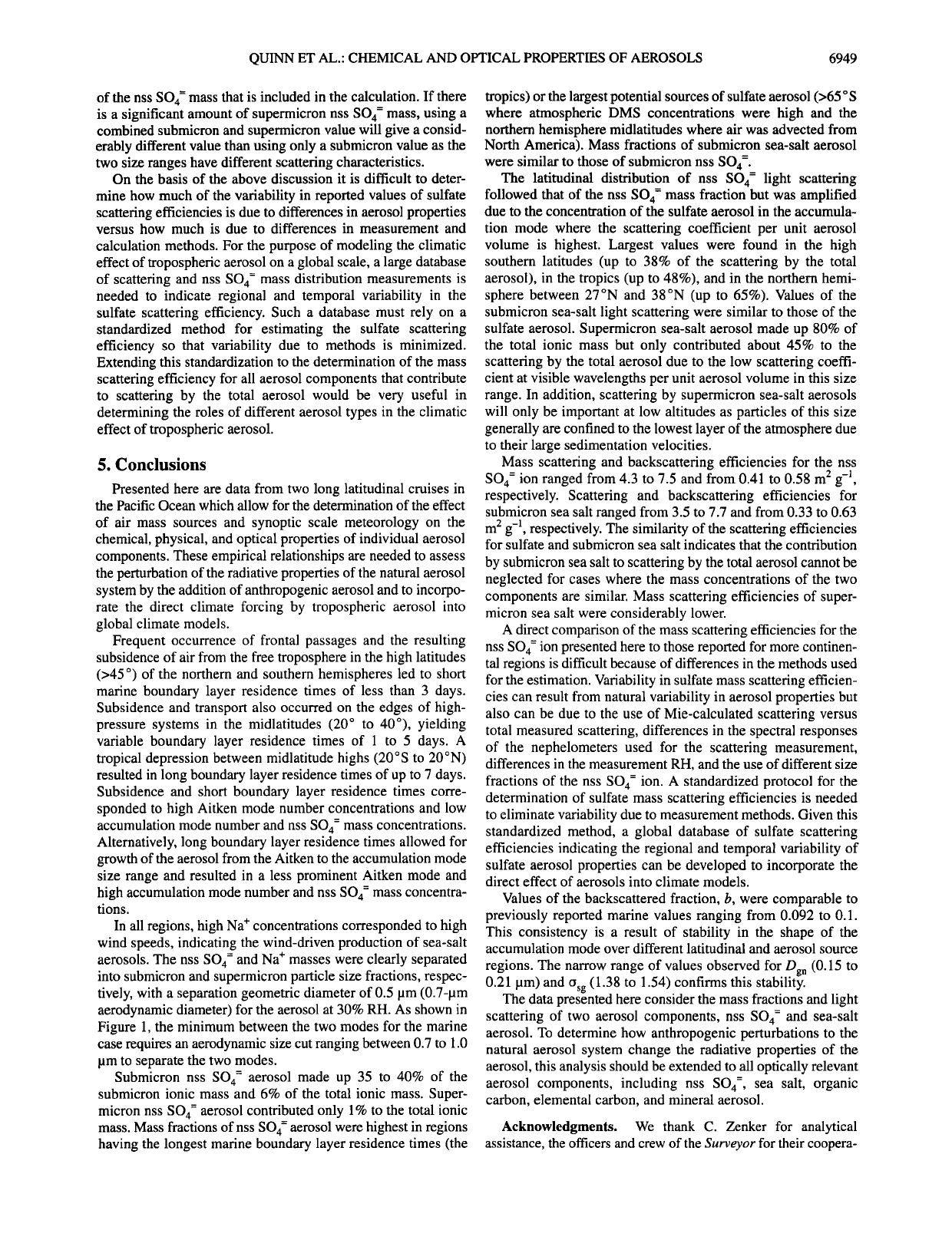
QUINN ET AL.: CHEMICAL AND OPTICAL PROPERTIES OF AEROSOLS 6949

of the nss SO4 = mass that is included in the calculation. If there

is a significant amount of supermicron nss SO4 = mass, using a

combined submicron and supermicron value will give a consid-

erably different value than using only a submicron value as the

two size ranges have different scattering characteristics.

On the basis of the above discussion it is difficult to deter-

mine how much of the variability in reported values of sulfate

scattering efficiencies is due to differences in aerosol properties

versus how much is due to differences in measurement and

calculation methods. For the purpose of modeling the climatic

effect of tropospheric aerosol on a global scale, a large database

of scattering and nss SO4 = mass distribution measurements is

needed to indicate regional and temporal variability in the

sulfate scattering efficiency. Such a database must rely on a

standardized method for estimating the sulfate scattering

efficiency so that variability due to methods is minimized.

Extending this standardization to the determination of the mass

scattering efficiency for all aerosol components that contribute

to scattering by the total aerosol would be very useful in

determining the roles of different aerosol types in the climatic

effect of tropospheric aerosol.

5. Conclusions

Presented here are data from two long latitudinal cruises in

the Pacific Ocean which allow for the determination of the effect

of air mass sources and synoptic scale meteorology on the

chemical, physical, and optical properties of individual aerosol

components. These empirical relationships are needed to assess

the perturbation of the radiative properties of the natural aerosol

system by the addition of anthropogenic aerosol and to incorpo-

rate the direct climate forcing by tropospheric aerosol into

global climate models.

Frequent occurrence of frontal passages and the resulting

subsidence of air from the free troposphere in the high latitudes

(>45 ø ) of the northern and southern hemispheres led to short

marine boundary layer residence times of less than 3 days.

Subsidence and transport also occurred on the edges of high-

pressure systems in the midlatitudes (20 ø to 40ø), yielding

variable boundary layer residence times of 1 to 5 days. A

tropical depression between midlatitude highs (20øS to 20øN)

resulted in long boundary layer residence times of up to 7 days.

Subsidence and short boundary layer residence times corre-

sponded to high Aitken mode number concentrations and low

accumulation mode number and nss SO4 = mass concentrations.

Alternatively, long boundary layer residence times allowed for

growth of the aerosol from the Aitken to the accumulation mode

size range and resulted in a less prominent Aitken mode and

high accumulation mode number and nss SO4 = mass concentra-

tions.

In all regions, high Na + concentrations corresponded to high

wind speeds, indicating the wind-driven production of sea-salt

aerosols. The nss SO4 = and Na + masses were clearly separated

into submicron and supermicron particle size fractions, respec-

tively, with a separation geometric diameter of 0.5 tam (0.7-tam

aerodynamic diameter) for the aerosol at 30% RH. As shown in

Figure 1, the minimum between the two modes for the marine

case requires an aerodynamic size cut ranging between 0.7 to 1.0

tam to separate the two modes.

Submicron nss SO4 = aerosol made up 35 to 40% of the

submicron ionic mass and 6% of the total ionic mass. Super-

micron nss SO4 = aerosol contributed only 1% to the total ionic

mass. Mass fractions of nss SO4 = aerosol were highest in regions

having the longest marine boundary layer residence times (the

tropics) or the largest potential sources of sulfate aerosol (>65 øS

where atmospheric DMS concentrations were high and the

northern hemisphere midlatitudes where air was advected from

North America). Mass fractions of submicron sea-salt aerosol

were similar to those of submicron nss SO4 =.

The latitudinal distribution of nss SO4-- light scattering

followed that of the nss SO4 = mass fraction but was amplified

due to the concentration of the sulfate aerosol in the accumula-

tion mode where the scattering coefficient per unit aerosol

volume is highest. Largest values were found in the high

southern latitudes (up to 38% of the scattering by the total

aerosol), in the tropics (up to 48%), and in the northern hemi-

sphere between 27øN and 38øN (up to 65%). Values of the

submicron sea-salt light scattering were similar to those of the

sulfate aerosol. Supermicron sea-salt aerosol made up 80% of

the total ionic mass but only contributed about 45% to the

scattering by the total aerosol due to the low scattering coeffi-

cient at visible wavelengths per unit aerosol volume in this size

range. In addition, scattering by supermicron sea-salt aerosols

will only be important at low altitudes as particles of this size

generally are confined to the lowest layer of the atmosphere due

to their large sedimentation velocities.

Mass scattering and backscattering efficiencies for the nss

SO4 = ion ranged from 4.3 to 7.5 and from 0.41 to 0.58 m 2 g-i,

respectively. Scattering and backscattering efficiencies for

submicron sea salt ranged from 3.5 to 7.7 and from 0.33 to 0.63

m 2 g-i, respectively. The similarity of the scattering efficiencies

for sulfate and submicron sea salt indicates that the contribution

by submicron sea salt to scattering by the total aerosol cannot be

neglected for cases where the mass concentrations of the two

components are similar. Mass scattering efficiencies of super-

micron sea salt were considerably lower.

A direct comparison of the mass scattering efficiencies for the

nss SO4 = ion presented here to those reported for more continen-

tal regions is difficult because of differences in the methods used

for the estimation. Variability in sulfate mass scattering efficien-

cies can result from natural variability in aerosol properties but

also can be due to the use of Mie-calculated scattering versus

total measured scattering, differences in the spectral responses

of the nephelometers used for the scattering measurement,

differences in the measurement RH, and the use of different size

fractions of the nss SO4 = ion. A standardized protocol for the

determination of sulfate mass scattering efficiencies is needed

to eliminate variability due to measurement methods. Given this

standardized method, a global database of sulfate scattering

efficiencies indicating the regional and temporal variability of

sulfate aerosol properties can be developed to incorporate the

direct effect of aerosols into climate models.

Values of the backscattered fraction, b, were comparable to

previously reported marine values ranging from 0.092 to 0.1.

This consistency is a result of stability in the shape of the

accumulation mode over different latitudinal and aerosol source

regions. The narrow range of values observed for Den (0.15 to

0.21 tam) and os• (1.38 to 1.54) confirms this stability.

The data presented here consider the mass fractions and light

scattering of two aerosol components, nss SO4 = and sea-salt

aerosol. To determine how anthropogenic perturbations to the

natural aerosol system change the radiative properties of the

aerosol, this analysis should be extended to all optically relevant

aerosol components, including nss SO4-, sea salt, organic

carbon, elemental carbon, and mineral aerosol.

Acknowledgments. We thank C. Zenker for analytical

assistance, the officers and crew of the Surveyor for their coopera-

6950 QUINN ET AL.: CHEMICAL AND OPTICAL PROPERTIES OF AEROSOLS

tion, and T. Anderson and R. Charlson for helpful comments. This

research was funded by the Ecology and Atmospheric Chemistry

Branch of the NASA Mission to Planet Earth Science Division and

by the Aerosol Component of the NOAA Climate and Global

Change Program. It is a contribution to the International Global

Atmospheric Chemistry (IGAC) Core Project of the International

Geosphere-Biosphere Programme (IGBP). This is NOAA PMEL

contribution 1645 and JISAO contribution 326.

References

Anderson, T. L., R. J. Charlson, W. H. White, and P. H. McMurry,

Comment on "Light scattering and cloud condensation nucleus

activity of sulfate aerosol measured over the Northeast Atlantic

Ocean" by D. A. Hegg et al., J. Geophys. Res., 99, 25,947-

25,949, 1994.

Andreae, M. O., The ocean as a source of atmospheric sulfur

compounds, in The Role of Air-Sea Exchange in Geochemical

Cycling, edited by P. Buat-Menard, pp. 331-362, D. Reidel,

Norwell, Mass., 1986.

Baron, P. A., Calibration and use of the aerodynamic particle sizer

(APS 3300), Aerosol Sci. Technol., 5, 55-67, 1986.

Barfie, L. A., and R. M. Hoff, Five years of air chemistry observa-

tions in the Canadian Arctic, Atmos. Environ., 19, 1995-2010,

1985.

Bates, T. S., J. D. Cline, R. H. Gammon, and S. R. Kelly-Hansen,

Regional and seasonal variations in the flux of oceanic

dimethylsulfide to the atmosphere, J. Geophys. Res., 92,

2930-2938, 1987.

Bates, T. S., K. C. Kelly, J. E. Johnson, and R. H. Gammon,

Regional and seasonal variations in the flux of oceanic carbon

monoxide to the atmosphere, J. Geophys. Res., 100, 23,093-

23,101, 1995.

Bemer, A., C. Lurzer, F. Pohl, O. Preining, and P. Wagner, The

size distribution of the urban aerosol in Vienna, Sci. Total

Environ., 13, 245-261, 1979.

Bodhaine, B. A., N. C. Ahlquist, and R. C. Schnell, Three-wave-

length nephelometer suitable for aircraft measurement of

background aerosol scattering coefficient, Atmos. Environ.,

25A, 2267-2276, 1991.

Bohren, C. F., and D. R. Huffman, Absorption and Scattering of

Light by Small Particles, John Wiley, New York, 1983.

Bray, W. H., Water vapor pressure control with aqueous solutions

of sulfuric acid, J. Mater., 5, 233-248, 1970.

Cantrell, B. K., and K. T. Whitby, Aerosol size distributions and

aerosol volume formation for a coal-fired power plant plume,

Atmos. Environ., 12, 323-333, 1978.

Clarke, A.D., Atmospheric nuclei in the Pacific midtroposphere:

Their nature, concentration, and evolution, J. Geophys. Res., 98,

20,633-20,647, 1993.

Covert, D. S., and J. Heintzenberg, Size distributions and chemical

properties of aerosol at Ny Alesund, Svalbard, Atmos. Environ.,

27A, 2989-2997, 1993.

Covert, D. S., V. N. Kapustin, T. S. Bates, and P. K. Quinn,

Physical properties of marine boundary layer aerosol particles

of the mid-Pacific in relation to sources and meteorological

transport, J. Geophys. Res., in press, 1995.

Draxler, R. R., Hybrid single-particle Lagrangian integrated

trajectories (HY-SPLIT): Version 3.0, User's Guide and Model

Description, Tech. Rep. ERL ARL-195, Natl. Oceanic and

Atmos. Admin., Silver Springs, Md., 1992.

Hegg, D. A., D. S. Covert, and V. N. Kapustin, Modeling a case of

particle nucleation in the marine boundary layer, J. Geophys.

Res., 97, 9851-9857, 1992.

Holland, H. D., The Chemistry of the Atmosphere and Oceans, p.

154, John Wiley, New York, 1978.

Hoppel, W. A., G. M. Frick, J. W. Fitzgerald, and R. E. Larson,

Marine boundary layer measurements of new particle formation

and the effect which nonprecipitating clouds have on the aerosol

size distribution, J. Geophys. Res., 99, 14,443-14,459, 1994.

Keady, P. B., F. R. Quant, and G. S. Sem, Differential mobility

particle sizer: A new instrument for high resolution aerosol size

distribution measurements below 1 pm, TSI Q., 9, 3-11, 1983.

Kent, G. S., et al., Modeling atmospheric aerosol backscatter at

CO 2 laser wavelengths, 1, Aerosol properties, modeling

techniques, and associated problems, Appl. Opt., 22, 1655-

1665, 1983.

Langner, J. and H. Rodhe, A global three-dimensional model of the

tropospheric sulfur cycle, J. Atmos. Chem., 13, 225-263, 1991.

Liu, B. Y. H., and K. W. Lee, Efficiency of membrane and

Nuclepore filters for submicrometer aerosols, Environ. Sci.

Technol., 10, 345-350, 1976.

Liu, B. Y. H., and D. Pui, On the performance of the electrical

aerosol analyzer, J. Aerosol Sci., 6, 249-264, 1975.

Marshall, S. F., Measurement-derived radiative transfer parameters

for the aerosol climate forcing problem, M.S. dissertation, Univ.

of Washington, Seattle, 1994.

Meszaros, A., and K. Vissy, Concentrations, size distribution and

chemical nature of atmospheric aerosol particles in remote

ocean areas, J. Aerosol Sci., 5, 101-109, 1974.

Mclnnes, L. M., D. S. Covert, and B. M. Baker, The number of

sea-salt sulfate and carbonaceous particles in the marine

atmosphere: Measurements consistent with the ambient size

distribution, in preparation, 1995a.

McInnes, L. M., P. K. Quinn, D. S. Covert, and T. L. Anderson,

Gravimetric analysis, ionic composition, and associated water

mass of the marine aerosol, Atmos. Environ., in press, 1995b.

Merrill, J., E. Arnold, M. Leinen, and C. Weaver, Mineralogy of

aeolian dust reaching the North Pacific Ocean, 2, Relationship

of mineral assemblages to atmospheric transport patterns, J.

Geophys. Res., 99, 21,025-21,032, 1994.

Monahan, E. C., The ocean as a source for atmospheric particles,

in The Role of Air-Sea Exchange in Geochemical Cycling,

edited by P. Buat-Menard, pp. 331-362, D. Reidel, Norwell,

Mass., 1986.

O'Dowd, C. D., and M. H. Smith, Physicochemical properties of

aerosols over the North Atlantic: Evidence for wind-speed-

related submicron sea-salt aerosol production, J. Geophys. Res.,

98, 1137-1149, 1993.

Plass-Dulmer, C., R. Koppmann, M. Ratte, and J. Rudolph, Light

nonmethane hydrocarbons in seawater, Global Biogeochem.

Cycles, 9, 79-100, 1995.

Pszenny, A. A. P., A. J. Castelie, R. A. Duce, and J. N. Galloway,

A study of the sulfur cycle in the Antarctic marine boundary

layer, J. Geophys. Res., 94, 9818-9830, 1989.

Quinn, P. K., T. S. Bates, J. E. Johnson, D. S. Covert, and R. J.

Charlson, Interactions between sulfur and reduced nitrogen

cycles over the central Pacific Ocean, J. Geophys. Res., 95,

16,405-16,416, 1990.

Quinn, P. K., D. S. Covert, T S. Bates, V. N. Kapustin, D.C.

Ramsey-Bell, and L. M. Mclnnes, Dimethylsulfide/cloud

condensation nuclei/climate system: Relevant size-resolved

measurements of the chemical and physical properties of

atmospheric aerosol particles, J. Geophys. Res., 98, 10,411-

10,427, 1993.

Quinn, P. K., S. F. Marshall, T S. Bates, D. S. Covert, and V. N.

Kapustin, Comparison of measured and calculated aerosol

properties relevant to the direct radiative forcing of tropospheric

sulfate aerosol on climate, J. Geophys. Res., 100, 8977-8992,

1995.

Rau, J. A., and M. A. K. Khalil, Anthropogenic contributions to the

carbonaceous content of aerosols over the Pacific Ocean, Atmos.

Environ., 27A, 1297-1307, 1993.

Reineking, A., and J. Porstendorfer, Measurements of particle loss

functions in a differential mobility analyzer for different flow

rates, Aerosol Sci. Technol., 5, 483-487, 1986.

Ruby, M. G., and A. P. Waggoner, Intercomparison of integrating

QUINN ET AL.: CHEMICAL AND OPTICAL PROPERTIES OF AEROSOLS 6951

nephelometer measurements, Environ. Sci. Technol., 15,

109-113, 1981.

Savoie, D. L., and J. M. Prospero, Particle size distribution of

nitrate and sulfate in the marine atmosphere, Geophys. Res.

Lett., 9, 1207-1210, 1982.

Sloane, C. S., J. Watson, J. Chow, L. Pritchett, and L. W. Richards,

Size-segregated fine particle measurements by chemical species

and their impact on visibility impairment in Denver, Atmos.

Environ., 25A, 1013-1024, 1991.

Stelson, A. W., Urban aerosol refractive index prediction by partial

molar refraction approach, Environ. Sci. Tech., 24, 1676-1679,

1990.

Stoiber, R. E., S. N. Williams, and B. Heubert, Annual contribution

of sulfur dioxide to the atmosphere by volcanos, J. Volcanol.

Geotherm. Res., 33, 1-8, 1987.

Tang, I. N., and H. R. Munkelwitz, Simultaneous determination of

refractive index and density of an evaporating aqueous solution

droplet, Aerosol. Sci. Technol., 15, 201-207, 1991.

Tang, I. N., and H. R. Munkelwitz, Water activities, densities, and

refractive indices of aqueous sulfate and nitrate droplets of

atmospheric importance, J. Geophys. Res., 99, 18,801-18,808,

1994.

ten Brink, H. M., S. E. Schwartz, and P. H. Daum, Efficient

scavenging of aerosol sulfate by liquid-water clouds, Atmos.

Environ., 21, 2035-2052, 1987.

Waggoner, A. P., A. J. Vanderpol, R. J. Charlson, S. Larsen, L.

Granat, and C. Tradgard, Sulfate light scattering ratio as an

index of the role of sulfur in the tropospheric optics, Nature,

261, 120-122, 1976.

Weiss, R. E., T. V. Larson, and A. P. Waggoner, In situ rapid-

response measurements of H2SO4/(NH4)2SO 4 aerosols in mral

Virginia, Environ. Sci. Technol., 16, 525-532, 1982.

Whitby, K. T., The physical characteristics of sulfur aerosols,

Atmos. Environ., 12, 135-159, 1978.

Whitby, K. T., and G. M. Sverdrup, California aerosols: Their

physical and chemical characteristics, Adv. Environ: Sci.

Technol., 10, 477-517, 1980.

Zang, Z., and B. Y. H. Liu, Performance of TS13760 condensation

nuclei counter at reduced pressures and flow rates, Aerosol Sci.

Technol., 15, 228-238, 1991.

Zhang, X., B. J. Turpin, P. H. McMurry, S. V. Hering, and M. R.

Stolzenburg, Mie theory evaluation of species contributions to

1990 wintertime visibility reduction in the Grand Canyon, J. Air

Waste Manage. Assoc., 44, 153-162, 1994.

T S. Bates, V. N. Kapustin, P. K. Quinn (corresponding author),

NOAA Pacific Marine Environmental Laboratory, 7600 Sand Point

Way N.E., Seattle, WA, 98115. (bates @pmel.noaa.gov; kapustin@

pmel.noaa.gov; [email protected])

D. S. Covert, Department of Atmospheric Sciences, University

of Washington, Seattle, WA 98195. ([email protected])

(Received June 22, 1995; revised October 27, 1995;

accepted November 1, 1995.)