A 3-year record of simultaneously measured
aerosol chemical and optical properties
at Barrow, Alaska
P. K. Quinn, T. L. Miller, and T. S. Bates
Pacific Marine Environmental Laboratory, NOAA, Seattle, Washington, USA
J. A. Ogren and E. Andrews
Climate Monitoring and Diagnostics Laboratory, NOAA, Boulder, Colorado, USA
G. E. Shaw
Geophysical Institute, University of Alaska, Fairbanks, Alaska, USA
Received 27 August 2001; revised 17 December 2001; accepted 7 January 2002; published 15 June 2002.
[1] Results are presented from 3 years of simultaneous measurements of aerosol chemical
composition and light scattering and absorption at Barrow, Alaska. All results are reported
at the measurement relative humidity of 40%. Reported are the annual cycles of the
concentration of aerosol mass, sea salt, non-sea-salt (nss) sulfate, methanesulfonate or
MSA
,NH
4
+
, and nss K
+
,Mg
+2
, and Ca
+2
for the submicron and supermicron size ranges.
Submicron nss SO
4
=
,NH
4
+
, and nss K
+
,Mg
+2
, and Ca
+2
peak in winter and early spring
corresponding to the arrival and persistence of Arctic Haze. Submicron sea salt displays a
similar annual cycle presumably due to long-range transport from the northern Pacific
Ocean. Supermicron sea salt peaks in summer corresponding to a decrease in sea ice
extent. Submicron and supermicron MSA
peak in the summer due to a seasonal increase
in the flux of dimethylsulfide from the ocean to the atmosphere. A correlation of MSA
and particle number concentrations suggests that summertime particle production is
associated with this biogenic sulfur. Mass fractions of the dominant chemical species were
calculated from the concentrations of aerosol mass and chemical species. For the
submicron size range the ionic mass and associated water make up 80 to 90% of the
aerosol mass from November to May. Of this ionic mass, sea salt and nss SO
4
=
are the
dominant species. The residual mass fraction, or fraction of mass that is chemically
unanalyzed, is equivalent to the ionic mass fraction in June through October. For the
supermicron size range the ionic mass and associated water make up 60 to 80% of the
aerosol mass throughout the year with sea salt being the dominant species. Also reported
for the submicron size range are the annual cycles of aerosol light scattering and
absorption at 550 nm, A
˚
ngstro¨m exponent for the 450 and 700 nm wavelength pair, and
single scattering albedo at 550 nm. On the basis of linear regressions between the
concentrations of sea salt and nss SO
4
=
and the light scattering coefficient, sea salt has a
dominant role in controlling light scattering during the winter, nss SO
4
=
is dominant in the
spring, and both components contribute to scattering in the summer. Submicron mass
scattering efficiencies of the dominant aerosol chemical components (nss SO
4
=
, sea salt,
and residual mass) were calculated from a multiple linear regression of the measured light
scattering versus the component concentrations. Submicron nss SO
4
=
mass scattering
efficiencies were relatively constant throughout the year with seasonal averages ranging
from 4.1 ± 2.9 to 5.8 ± 1.0 m
2
g
1
. Seasonal averages for submicron sea salt ranged from
1.8 ± 0.37 to 5.1 ± 0.97 m
2
g
1
and for t he residual mass ranged from 0.21 ± 0.31 to 1.5 ±
1.0 m
2
g
1
. Finally, concentrations of nss SO
4
=
measured at Barrow were compared to
those measured at Poker Flat Rocket Range, Denali National Park, and Homer for the
1997/1998 and 1998/1999 Arctic Haze seasons. Concentrations were highest at Barrow
and decreased with latitude from Poker Flat to Denali to Homer revealing a north to south
JOURNAL OF GEOPHYSICAL RESEARCH, VOL. 107, NO. D11, 10.1029/2001JD001248, 2002
Copyright 2002 by the American Geophysical Union.
0148-0227/02/2001JD001248$09.00
AAC 8 - 1
gradient in the extent of the haze. INDEX TERMS: 0305 Atmospheric Composition and Structure:
Aerosols and particles (0345, 4801); 0365 Atmospheric Composition and Structure: Troposphere—
composition and chemistry; 1610 Global Change: Atmosphere (0315, 0325); K
EYWORDS: Arctic, aerosol,
chemistry, optics, time series
1. Introduction
[2] The late winter-early spring maximum in aerosol light
scattering, absorption, and mass concentration at Barrow is
a well-documented phenomenon known as Arctic Haze.
Several seasonal variations contribute to the development of
Arctic Haze including stronger transport from the midlati-
tudes to the Arctic [e.g., Shaw, 1981; Barrie et al., 1989;
Iversen and Joranger, 1985] and weaker pollutant removal
through wet deposition in the winter and spring [e.g., Barrie
et al., 1981; Shaw, 1981; Heintzenberg and Larssen, 1983].
Arctic Haze has been the subject of much study as it may
change the solar radiation balance of the Arctic, affect
visibility, and provide a source of contaminants to Arctic
ecosystems.
[
3] The goals of the National Oceanic and Atmospheric
Administration’s (NOAA) regional-scale aerosol monitor-
ing program are to characterize means, variabilities, and
trends of climate-forcing properties of different aerosol
types and to understand the f actors that control these
properties. Current North American monitoring sites are
located at Barrow, Alaska, Southern Great Plains, Okla-
homa, and Bondville, Illinois. This paper focuses on simul-
taneous measurements of aerosol chemical and optical
properties made at B arrow (71.32N, 156.61W) from
October 1997 to December 2000. Seasonal changes in
aerosol composition are determined along with the effect
of these changes on optical properties.
[
4] NOAA began aerosol observations at Barrow in 1976
using an integrating nephelometer to measure aerosol light
scattering and a condensation nucleus counter to measure
aerosol number concentration. In 1988 an aethalometer was
added to measure light absorption by particles. Results from
these measurements have been reported previously [e.g.,
Polissar et al., 1999; Bodhaine, 1995; Bodhaine and
Dutton, 1993; Bodhaine, 1989]. In 1997 several changes
were made to the aerosol observing system. A high-sensi-
tivity nephelometer (TSI m odel 3563) was installed, a
continuous light absorption photometer (PSAP, Radiance
Research) supplanted the aethalometer, the aerosol inlet was
modified to control the relative humidity (RH) of the
sampled air, and sector-controlled sampling was imple-
mented to eliminate sampling of the locally polluted sector.
In addition, routine and continuous collection of aerosol for
chemical analysis (major ions and aerosol mass) was begun
with an automated filter sampling system. Aerosol collected
for chemical anal ysis is segregated into submicron and
supermicron size fractions. The size segregation allows for
the differentiation of aerosol that is transported over long
distances (submicron size range which contains the accu-
mulation mode) and locally generated aerosol that has a
relatively short lifetime (supermicron size range which
contains the coarse mode).
[
5] Reported here for the first time are results from the
continuous sampling of chemic al and optical properties
using the upgraded aerosol sampling system. This data
record is the longest reported of simultaneous, year-round
measurements of aerosol chemical and optical properties at
Barrow. Presented are monthly mean concentrations of
aerosol mass and the dominant aerosol ionic chemical
components, monthly mean values of aerosol light scatter-
ing and absorption coefficients, single scattering albedo,
A
˚
ngstro¨m exponent, and particle number concentration. We
relate chemical and optical properties for the winter (Octo-
ber to January), spring (March to June), and summer (July
to September) seasons through linear regressions of the light
scattering coefficient against the mass concentrations of sea
salt and non-sea-salt SO
4
=
. In addition, we report mass
scattering efficiencies, the parameter which directly links
the mass concentration of a chemical component with its
light scattering efficiency, for submicron aerosol mass, sea
salt, and nss SO
4
=
. Finally, we compare the aerosol chemical
composition measured at Barrow to that measured at three
more southerly sites in Alaska to determine how far south
Arctic Haze extended during the 1997/1998 and 1998/1999
haze seasons. The three sites are Poker Flat Rocket Range,
Denali National Park, and Homer.
[
6] All measurements reported here were made at the
surface. Aerosol concentrations in haze layers aloft can be
much larger than surface concentrations due to the stability
of the Arctic atmosphere [e.g., Schnell et al., 1989]. During
weaker i nversions or when the inversion breaks down,
aerosol may be transported vertically, and surface and aloft
aerosol properties can be similar [Bodhaine, 1989]. During
periods of a strong inversion, however, surface and aloft
aerosol loadings and properties are not well correlated.
Therefore it is acknowledged that measurements at the
surface do not always represent the entire atmospheric
column. At this time, however, continuous observations at
the surface offer the most cost-effective method for identi-
fying seasonal, annual, and longer-term trends and cycles
[Hopper et al., 1994].
2. Measurements at Barrow
[7] Sample air is drawn into a 21.6 cm inner diameter
inlet stack at 10 m above ground level [Delene and Ogren,
2002]. The flow rate through the stack is approximately
1000 L min
1
and is divided into a sample flow of 150 L
min
1
and a sheath flow of 850 L min
1
. The sample flow
is taken from the center of the stack tube and drawn through
a 4.45 cm inner diameter stainless steel tube where the air is
heated to achieve a relative humidity of no more than 40%.
The sample flow is then split into five 1.6 cm inner diameter
lines each operating at a flow rate of 30 L min
1
. These
lines fe ed the different aerosol instruments which are
housed in a temperature-controlled building. Sampling is
sector- controlled such that real-time wind speed and
direction measured at the top of the inlet are used to exclude
data from the locally polluted sector (130 to 360).
[
8] Sample relative humidity (RH) is measured after the
heater and directly upstream of the aerosol instruments. The
amount of heating required to maintain this low reference
AAC 8 - 2 QUINN ET AL.: CHEMICAL AND OPTICAL PROPERTIES AT BARROW, ALASKA

RH varies with season. From 1997 through 2000, heating
averaged 31 ±8C in spring, 14 ±3C in summer, 25 ±
8C in fall, and 38 ±7C in winter to mai ntain a sample
RH between 20 and 40%. The aerosol is heated to maintain
a relatively stable reference RH that allows for constant
instrumental size segregation in spite of variations in
ambient RH. Chemical, physical, and optical measurements
are all made at this reference RH and thus are all directly
comparable. In addition, measurement at a low reference
RH makes it possible, with the knowledge of appropriate
growth factors, for end users of the data set (process,
chemical transport, and radiative transfer models) to adjust
the measured parameters to a desired relative humidity. All
measurements are reported at the reference RH.
[
9] The sample air for determination of aerosol chemical
composition and mass concentration first enters a Berner-
type multijet cascade impactor [Berner et al., 1979] with
aerodynamic D
50
cutoff diameters of 10 and 1 mm. A 12
mm grease cup is coated with silicone grease, and a film
coated with silicone spray is placed on the 10 mm jet place
to minimize bounce of large particles onto the downstream
stages. Particles with aerodynamic diameters between 1
and 10 mm are collected on a Tedlar film. Particles with
diameters less than 1 mm pass through the impactor to a
filter carousel housing 8 Millipore Fluoropore filters (1.0
mm pore size). Computer-controlled solenoid valves down-
stream of the filters open and close sequentially so that one
filter is sampled at a time. Submicron filter samples are
collected over a period of 1 to 5 days depending on the
time of year and the aerosol loading. One filter serves as a
sampling blank and is exposed to sample air for 10 s. One
supermicron sample is collected with the impactor during
the time it takes to sample all of the submicron filters in
the carousel. All handling of the impactor films and
carousel filters is done in a glove box purged with air that
has passed through a scrubber containing potassium car-
bonate and citric acid to remove SO
2
and NH
3
. After
collection, samples are shipped to NOAA’s Pacific Marine
Environmental Laboratory (PMEL) for analysis in sealed
tubes.
[
10] At PMEL the films and filters are wetted with 1 mL
of spectral grade methanol. An additional 5 mL of distilled
deionized water are added to the solution, and the substrates
are extracted by sonicating for 30 min. Concentrations of
major cations (Na
+
,NH
4
+
,K
+
,Mg
2+
,Ca
2+
) and anions
(methanesulfonate or MSA
,Cl
,NO
3
,SO
4
=
) are deter-
mined by ion chromatography [Quinn et al., 1998]. All
handling of substrates is done in a glove box similar to that
at Barrow. NO
3
concentrations are not reported because of
the uncertainties associated with heating of the aerosol to
maintain a sample RH below 40%. Heating by the amounts
required (an average of 14C in summer to 38C in winter)
may lead to substantial volatilization of ammonium nitrate
from the substrate resulting in artificially low nitrate con-
centrations [Meyer et al., 1992; Ayers et al., 1999].
[
11] Non-sea-salt sulfate (nss SO
4
=
) concentrations are
initially calculated from Na
+
concentrations and the mass
ratio of sulfate to sodium in seawater of 0.252 [Holland,
1978]. Negative nss SO
4
=
concentrations resulting from this
approach have been reported for Antarctic winter aerosol
[e.g., Wagenbach et al., 1988, 1998] and have been
attributed to depletion of sea salt SO
4
=
through fractiona-
tion processes. On the basis of sulfur isotope analysis, sea
salt SO
4
=
depletion also has been reported for the Canadian
Arctic [Norman et al., 1999]. Calculation of nss SO
4
=
for
the submicron size range using the SO
4
=
to Na
+
seawater
mass ratio of 0.252 did not yield negative values. There-
fore this approach was used for the submicron size range.
Negative nss SO
4
=
concentrations did result for the super-
micron size range, however. As per the method of Wagen-
bach et al. [1998], supermicron nss SO
4
=
concentrations
were calculated by performing a linear regression of nss
SO
4
=
calculated using the 0.252 mass ratio versus Na
+
for
the winter, spring, and summer seasons. The obta ined
negative slope was then added to the conventional ratio
of 0.252. Resulting supermicron SO
4
=
to Na
+
seawater
mass ratios were 0.13 for winter (October to February),
0.082 for spring (March to June), and 0.23 for summer
(July to September).
[
12] For the compar ison of Barrow and Alert nss SO
4
=
seasonal cycles, the submicron and supermicron Barrow
concentrations were summed for a more direct comparison
to the high-volume, non-size-segregated Alert samples.
(Seven day aerosol samples were collected at Alert on 20
cm by 25 cm Whatman 41 filters using a high-volume
sampler [Sirois and Barrie, 1999]. The face velocity of
sampling (50 cm s
1
) and typical filter l oadings ensured
collection efficiencies better than 95% [Watts et al., 1987]).
Alert nss SO
4
=
concentrations were calcula ted using the
0.252 SO
4
=
to Na
+
mass ratio since this did not yield any
negative nss SO
4
=
concentrations.
[
13] Sea salt aerosol concentrations are calculated as
sea salt mgm
3
¼ Cl
mgm
3
þ Na
þ
mgm
3
1:47; ð1Þ
where 1.47 is the seawater ratio of (Na
+
+K
+
+Mg
+2
+
Ca
+2
+SO
4
=
+ HCO
3
)/Na
+
[Holland, 1978]. Cl
in excess
of the Cl
to Na
+
seawater ratio of 1.8 was not added to the
sea salt mass. This approach prevents the inclusion of nss
K
+
,Mg
+2+
,Ca
+2
,SO
4
=
, and HCO
3
in the sea salt mass and
allows for the loss of Cl
mass through Cl
depletion
processes. It also assumes that all Na
+
is derived from
seawater. Results of Barrie and Barrie [1990] indicate that
the majority of Na
+
in the Arctic is associated with sea salt
that is either unmodified or anthropogenically modified.
[
14] All ion concentrations are reported at 0C and 1013
mbar. Throughout the paper, submicron refers to particles
with aerodynamic diameters ( D
aero
) less than 1 mm, and
supermicron refers to particles with aerodynamic diameters
Table 1. Distributions of Trajectories as Percentages Arriving at
Barrow From Six Di fferent Source Regions for the Winter
(October to January), Spring (March to June), and Summer (July
to September) Seasons
a
Source Region October – January March – June July – September
East Arctic Basin 27 18 17
North America 16 17 13
Pacific 7.8 23 22
Russia 5.2 2.5 1.4
Siberia 18 14 15
West Arctic Basin 27 25 31
a
The back trajectories were calculated twice daily for an arrival height of
500 m.
QUINN ET AL.: CHEMICAL AND OPTICAL PROPERTIES AT BARROW, ALASKA AAC 8 - 3

1.0 < D
aero
<10mm at the sample RH of 40%. Un-
certainties at the 95% confidence level for a typical low
and high concentration for each ionic species are given in
Table 2. Uncertainties in the ionic species include errors
due to the ion chromatography analysis, blank levels, the
volume of the liquid extract, and the volume of the air
sampled. All uncertainties shown in Table 2 were propa-
gated as a quadratic sum of all errors involved which
assumes that all errors were random. Details of the
uncertainty analysis are given by Quinn et al. [2000].
[
15] Submicron aerosol mass concentrations are deter-
mined by weighing the Millipore filters at PMEL before and
after sample collection with a Mettler UMT2 microbalance
[Quinn et al., 2000]. Supermicron aerosol mass concen-
trations are determined by weighing the Tedlar films with a
Cahn Model 29 m icrobalance. Both microbalances are
housed in a glove box kept at 33 ± 3% RH. Maintaining
the glove box at a constant RH allows each sampled
substrate to come into equilibrium with the same vapor
pressure of water, thus reducing experimental uncertainty
due to variable laboratory RH. The reported mass concen-
trations include the water mass that is associated with the
aerosol on the filter at the glove box RH. All aerosol mass
concentrations are reported at 0C, 1013 mbar, and the
sample RH. Uncertainties at the 95% confidence level for a
typical low and high mass concentration are given in
Table 2. Uncertainties in the aerosol mass include errors
due to weighing, blank levels, storage and transport, and the
volume of air sampled [Quinn et al., 2000].
[
16] Residual mass concentrations, or the mass of the
chemically unanalyzed species, were calculated from the
gravimetrically determined aerosol mass less the mass of the
ionic species and water. Uncertainties at the 95% confidence
level for a typical high and low residual mass concentration
are given in Table 2. Uncertainties in the residual mass
include errors due to the concentrations of the ionic species,
the aerosol mass, and water [Quinn et al., 2000].
[
17] Measurements of aerosol scattering coefficients were
made at wavelengths of 450, 550, and 700 nm at an RH
between 20 and 40% with a TSI 3563 nephelometer [Delene
and Ogren, 2002]. Two Berner-type impactors are operated
upstream of the nephelometer. The sample airflow is
switched every 5 min between the two impactors so that
scattering by either submicron or sub-10 mm particles is
measured. Values measured directly by the nephelometer
are corrected as per Anderson and Ogren [1998] for an
offset determined by measuring filtered air and for angular
nonidealities of the nephelometer including truncation
errors and nonlambertian response. Values are reported at
0C, 1013 mbar, and the sample RH.
[
18] The uncertainty associated with the scattering meas-
urements include errors due to noise, calibration, angular
nonidealities, and adjustment to STP. Using the method of
Anderson and Ogren [1998], the overall uncertainty of the
light scattering coefficient at 550 nm was estimated to be
7.8% for a 24-hour averaging time.
[
19] Aerosol absorption coefficients are measured by
monitoring the change in transmission through a filter with
a Particle Soot Absorption Photometer (PSAP, Radiance
Research). The PSAP is located downstream of the impac-
tors to determine both submicron and sub-10 mm absorption
coefficients. Measured values are corrected for a scattering
artifact, the deposit spot size, the PSAP flow rate, and the
manufacturer’s calibration as per Bond et al. [1999]. Values
are reported at 550 nm, 0C, 1013 mbar, and the sample
RH. The uncertainty associated with the absorption meas-
urements inc lude errors due to calibration, noise, and
adjustment to STP and 550 nm. Using the method of Bond
et al. [1999], the overall uncertainty of the absorption
coefficient at 550 nm was estimated to be 22% for a 24-hour
averaging time. Scattering and absorption coefficients were
averaged over the period of the submicron filter samples
and include only times when sample air was drawn through
the filters.
Table 2. Submicron Mass Concentrations at Barrow, Alaska, for October 1997 to December 2000
a
mgm
3
Mass
b
Sea Salt
c
nss SO
4
=d
NH
4
+e
MSA
f
nss K
+g
nss Mg
+2h
nss Ca
+2i
Residual
j
Jan. 3.8 ± 2.2 1.1 ± 1.1 0.78 ± 0.43 0.23 ± 0.09 <0.0001 0.03 ± 0.03 0.09 ± 0.11 0.03 ± 0.03 0.62 ± 1.0
Feb. 3.5 ± 1.7 0.93 ± 1.1 0.91 ± 0.39 0.26 ± 0.09 <0.0001 0.03 ± 0.02 0.06 ± 0.07 0.02 ± 0.03 0.56 ± 0.57
March 2.6 ± 1.3 0.68 ± 0.73 0.71 ± 0.44 0.21 ± 0.12 <0.0001 0.02 ± 0.01 0.03 ± 0.04 0.01 ± 0.01 0.41 ± 0.69
April 2.1 ± 1.1 0.43 ± 0.61 0.72 ± 0.36 0.19 ± 0.07 0.002 ± 0.002 0.01 ± 0.01 0.008 ± 0.01 0.003 ± 0.005 0.32 ± 0.40
May 1.2 ± 0.60 0.15 ± 0.15 0.60 ± 0.50 0.14 ± 0.06 0.01 ± 0.01 0.005 ± 0.004 0.002 ± 0.003 0.006 ± 0.009 0.08 ± 0.10
June 0.89 ± 1.1 0.05 ± 0.10 0.19 ± 0.21 0.06 ± 0.05 0.01 ± 0.02 0.002 ± 0.002 0.0003 ± 0.0006 0.004 ± 0.008 0.45 ± 1.1
July 0.60 ± 0.49 0.08 ± 0.09 0.10 ± 0.10 0.03 ± 0.03 0.01 ± 0.01 0.001 ± 0.001 <0.0001 0.005 ± 0.01 0.27 ± 0.25
Aug. 0.81 ± 0.82 0.17 ± 0.22 0.08 ± 0.06 0.02 ± 0.01 0.01 ± 0.01 0.001 ± 0.001 <0.0001 0.001 ± 0.002 0.40 ± 0.33
Sept. 0.61 ± 0.44 0.17 ± 0.11 0.09 ± 0.12 0.02 ± 0.04 0.007 ± 0.004 0.001 ± 0.001 <0.0001 0.002 ± 0.005 0.26 ± 0.37
Oct. 2.0 ± 1.6 0.74 ± 0.98 0.13 ± 0.16 0.05 ± 0.06 0.0009 ± 0.001 0.002 ± 0.007 0.0003 ± 0.001 0.02 ± 0.07 0.93 ± 1.2
Nov. 1.4 ± 1.2 0.62 ± 0.86 0.13 ± 0.09 0.05 ± 0.04 0.0002 ± 0.0005 0.003 ± 0.006 0.001 ± 0.003 0.009 ± 0.02 0.30 ± 0.45
Dec. 3.1 ± 3.0 1.1 ± 1.2 0.32 ± 0.23 0.09 ± 0.05 0.0001 ± 0.0003 0.01 ± 0.01 0.02 ± 0.02 0.009 ± 0.01 0.55 ± 0.44
a
Concentrations are reported as arithmetic mean and standard deviation (1s)at0C and 1013 mbar.
b
Uncertainties for low and high concentrations of mass are 0.6 ± 5.5% and 3.0 ± 5.2% mgm
3
(concentration ± 95% uncertainty).
c
Uncertainties for low and high concentrations of sea salt are 0.2 ± 9.6% and 1.0 ± 6.1% mgm
3
(concentration ± 95% uncertainty).
d
Uncertainties for low and high concentrations of nss SO
4
=
are 0.05 ± 7.0% and 1.0 ± 6.0% mgm
3
(concentration ± 95% uncertainty).
e
Uncertainties for low and high concentrations of NH
4
+
are 0.01 ± 39% and 0.2 ± 7.8% mgm
3
(concentration ± 95% uncertainty).
f
Uncertainties for low and high concentrations of MSA
are 0.0005 ± 6.0% and 0.01 ± 6.0% mgm
3
(concentration ± 95% uncertainty).
g
Uncertainties for low and high concentrations of nss K
+
are 0.001 ± 14% and 0.03 ± 6.1% mgm
3
(concentration ± 95% uncertainty).
h
Uncertainties for low and high concentrations of nss Mg
+2
are 0.0005 ± 16% and 0.09 ± 6.2% mgm
3
(concentration ± 95% uncertainty).
i
Uncertainties for low and high concentrations of nss Ca
+2
are 0.004 ± 69% and 0.03 ± 48% mgm
3
(concentration ± 95% uncertainty).
j
Calculated from the gravimetric mass less the ionic mass and associated water. Uncertainties for low and high concentrations of residual mass are 0.3 ±
51% and 1.0 ± 21% mgm
3
(concentration ± 95% uncertainty). Uncertainties for low and high concentrations of H
2
O are 0.11 ± 33% and 3.0 ± 5.3% mg
m
3
(concentration ± 95% uncertainty) at 33% RH.
AAC 8 - 4 QUINN ET AL.: CHEMICAL AND OPTICAL PROPERTIES AT BARROW, ALASKA
[20] Aerosol number concentration is measured with a
TSI model 3760 condensation particle counter. The reported
number concentration includes all particles with diameters
greater than 14 nm at the sample RH. Number concentra-
tions were averaged over the period of the daily submicron
filter samples and include only times when sample air was
drawn through the filters.
[
21] Air mass back trajectories were calculated for three
arrival heights (500, 2500, and 5500 m) for the station
location at 12-hour intervals. Trajectories were calculated
with the Hybrid Single-Particle Lagrangian Integrated Tra-
jectory (HY-SPLIT 4) model based on the FNL global wind
field [Draxler, 1992].
[
22] The gravimetric analysis was performed at 33% RH.
Hence the measured mass on the sampling substrates
included the amount of water associated with the aerosol
at that RH. The chemical thermodynamic equilibrium model
AeRho [Quinn et al., 1998] was used to estimate the water
mass associated with the inorganic ions at 33% RH so that
mass fractions of the aerosol chemical components could be
calculated from the gravimetric and ionic mass. Uncertain-
ties at the 95% confidence level are reported for a typical
low and high H
2
O concentration in Table 2. Uncertainties in
the water calculation include errors due to the measured
chemical composition, the glove box RH and temperature,
and the volume of air sampled. See Quinn et al. [2000] for
details of the uncertainty calculations.
[
23] AeRho is a static model. It is designed to take the
measured ionic composition of the aerosol and the constant
sampling RH and to determine the molecular compo sition
of the ionic chemical species within the aerosol. The
molecular composition then is used to calculate the water
mass associated with the aerosol species. The model is not
used to describe a dynamic system in which changes in the
concentration of gas phase species affect the aerosol molec-
ular composition. Therefore it does not include interactions
between the gas and aqueous phases. In addition, because of
the constant sampling RH, it is not necessary to take into
account changes in particle size with changes in RH. More
details about the model are given by Quinn et al. [1998] and
Quinn and Coffman [1998].
3. Results: Trajectory Analysis
[24] As pointed out by Lowentha l and Rahn [1985], the
use of trajectories to reconstruct the history of sampled air
masses in the Arctic is difficult because of the large
distances to the source regions (5000 to 10,000 km or 5
to 20 days transit time) and sparse meteorological data.
Knowing the limits of Arctic trajectory analysis, twice daily
back trajectories were calculated to determine if a seasonal
patt ern existed in source regions to Barrow during the
October 1997 to Dec embe r 2000 measurement period.
Trajectories calculated 7 days back in time and arriving at
a height of 500 m were initially grouped into eight source
regions including the East Arctic Basin (0 to 180E and
north of contiguous landmasses), West Arctic Basin (0 to
180W and north of contiguous landmasses), North Amer-
ica, the Pacific Ocean, Russia (30 Eto90E), Siberia (90E
to eastern edge of Russia), Europe, and the Atlantic Ocean.
Because of the scarcity of trajectories from Europe and the
Atlantic, the number of source regions was reduced to six.
[
25] Table 1 shows the distributions of the source regions
for winter (October to January), spring (March to June), and
summer (July to September). The data were segregated
based on similarities in the submicron nss SO
4
=
and sea salt
concentrations for these time periods. February was not
included as it appeared to be a transitional month between
the winter and spring season s. The large frequency of
trajectories from the East and West Arctic Basins indicates
that 7 day back trajectories often do not allow for the
determination of the source region. Unfortunately, accuracy
of the trajectory analysis decreases with each day back in
time. Seasonal differences are not large, but it is apparent
that winter has the fewest trajectori es from North America
and the Pacific and the most from the East Arctic Basin,
Russia, and Siberia. On the basis of trace elemental analysis,
midlatitude regions in Russia and Siberia have been iden-
tified as significant sources of pollutant aerosol to the Arctic
[Rahn, 1981a, 1981b; Lowenthal and Rahn, 1985]. Distri-
butions of source regions for spring and summer are not
significantly different. Of those trajectories traveling back to
Russia and Siberia, a higher percentage traveled more than
4000 km during the winter (50%) than during the spring
(30%) or summer (20%). This analysis suggests that Arctic
Haze results from winter and spring episodic injections of
pollutant aerosols from the midlatitudes to the Arctic. These
aerosols then pool in the Arctic Basin since removal by wet
deposition is slow during this time of year. These results are
in agreement with those previously published [e.g., Bridg-
man and Bodhaine, 1994; Barrie et al., 1981].
4. Results: Chemical Composition
4.1. Mass Fractions of Ionic Components
[
26] Since the chemical analysis included only ionic
species, measureme nts of the concentrations of these
species and the total aerosol mass were used to determine
what fraction of the aerosol mass was being taken into
account. Mass fractions of the submicron and supermi-
cron ionic chemical components were calculated as the
mass concentration of the component divided b y the
gravimetric mass. Shown in Figures 1 and 2 are percen-
tile information for the submicron and supermicron mass
fractions of the ionic mass (including associated water at
33% RH), sea salt, nss SO
4
=
,H
2
O calculated by AeRho to
be associated with the ionic species at 33% RH, and the
residual mass. The residual mass is defined as the
gravimetric mass less the mass of the ionic components
and associated water. Sea salt, nss SO
4
=
, and the residual
component dominate the aerosol mass. The remaining
ionic species (MSA
, nss K
+
, nss Mg
+2
, and nss Ca
+2
),
although useful tracers of the source of the aerosol,
contribute less than 10 and 4% to the aerosol submicron
and supermicron mass, respectively. NH
4
+
contributes, on
average, 6.5 ± 4.4% (arithmetic mean and 1s standard
deviation), 11 ± 4.3%, and 4.2 ± 2.9% to the submicron
mass during the winter (October to January), spring
(March to June), and summer (July to September),
respectively. NH
4
+
contributes, on average, less than 1%
to the supermicron mass.
[
27] The ionic mass and associated water make up 80 to
100% of the submicron aerosol mass during the months of
November to May (Figure 1). Of this ionic mass, sea salt
QUINN ET AL.: CHEMICAL AND OPTICAL PROPERTIES AT BARROW, ALASKA AAC 8 - 5
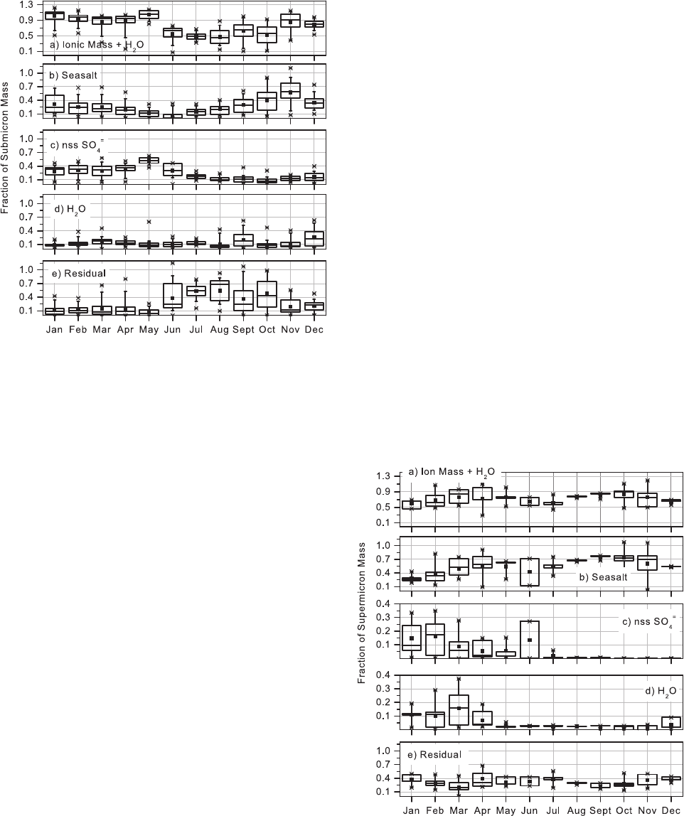
and nss SO
4
=
are the dominant species. The sea salt mass
fraction is larger than that of nss SO
4
=
during the winter
months (October to January). Sea salt and nss SO
4
=
mass
fractions are comparable in February and March, and the
nss SO
4
=
mass fraction is larger in April through June. The
residual mass fraction is less than 20% during November to
May but becomes comparable to the ionic mass fraction in
June through October. Particulate organic matter most likely
is a large component of the residual mass. Li and Win-
chester [1989] measured the aerosol chemical composition
at Barrow from March to May 1986 and found that con-
tributions of organic acid anions (formate, acetate, propio-
nate, and pyruvate) and inorganic anions to the aerosol mass
were comparable. The higher residual mass fractions meas-
ured during the summer most likely are of biogenic origin
since there is no strong source of anthropogenic aerosol
during this time of year.
[
28] On the basis of monthly averages the ionic mass
and associated water make up 60 to 80% of the super-
micron aerosol mass throughout the year (Figure 2). Of the
ionic mass, sea salt is the dominant species, contributing
60 to 98% on a monthly basis. The largest contribution
(>90%) of sea salt to the ionic mass occurs between July
and December. Non-sea-salt SO
4
=
makes a relatively small
contribution to the supermicron aerosol mass. It contrib-
utes, on a monthly basis, less than 1 to 16% with the
largest contributions in the late winter/early spring months.
The mass fraction of residual mass is fairly constant
throughout the year with monthly averages ranging from
20 to 39%. Again, based on the results of Li and Win-
chester [1989], organic species most likely comprise a
large portion of this residual mass.
4.2. Seasonal Cycles of the Dominant
Ionic Chemical Components
[
29] Sea salt aerosol results from the wind-driven pro-
duction and subsequent evaporation of sea spray. Submi-
cron sea salt concentrations increase in October, peak in
December and January, begin a steady decrease in February,
and reach lowest concentrat ions in the summer months of
May through Se ptemb er (Figure 3b). Du ring the peak
months of December and January, mean submicron con-
centrations equal 1.1 ± 1.1 mgm
3
(arithmetic mean and 1s
standard deviation) (Table 2). Supermicron sea salt concen-
trations display a very different seasonal cycle with con-
centrations increasing in July, peaking in August to October,
and decreasing in November and December (Figure 4b).
Lowest concentrations are observed in January throu gh
June. During the peak months the arithmetic mean of the
Figure 1. Box plots of submicron mass fractions of (a)
ionic mass (includes sea salt, nss SO
4
=
, nss K
+
, nss Mg
+2
,
nss Ca
+2
,NH
4
+
, MSA
,Cl
not associated with sea salt,
NO
3
, and water associated with the ionic components at
33% RH), (b) sea salt, (c) nss SO
4
=
, (d) water associated
with the ionic components at 33% RH, and (e) residual mass
(calculated as gravimetric mass less the mass of ionic
species and associated water). The horizontal lines in the box
denote the 25th, 50th, and 75th percentile values. The error
bars denote the 5th and 95th percentile values. The two
symbols below the 5th percentile error bar denote the 0th
and 1st percentile values, and the two symbols above the
95th percentile error bar denote the 99th and 100th
percentiles. The square symbol in the box denotes the
arithmetic mean.
Figure 2. Box plots of supermicron mass fractions of (a)
ionic mass (includes sea salt, nss SO
4
=
, nss K
+
, nss Mg
+2
,
nss Ca
+2
,NH
4
+
, MSA
,Cl
not associated with sea salt,
NO
3
, and water associated with the ionic components at
33% RH), (b) sea salt, (c) nss SO
4
=
, (d) water associated
with the ionic components at 33% RH, and (e) residual mass
(calculated as gravimetric mass less the mass of ionic
species and associated water). Percentile information is as in
the Figure 1 caption.
AAC 8 - 6 QUINN ET AL.: CHEMICAL AND OPTICAL PROPERTIES AT BARROW, ALASKA
supermicron concentration ranges from 1.4 to 2.1 mgm
3
(Table 3).
[
30] The winter maximum in Arctic submicron sea salt
concentrations has been attributed to seasonally high winds
in high-latitude source regions of the Pacific and Atlantic
Oceans and long-range transport to the Arctic [Sturges and
Barrie, 1988; Sirois and Barrie, 1999; Quinn et al., 2000].
Maximum supermicron sea salt concentrations at Barrow
occur during the summer when the ice pack extent is at a
minimum. In addition, long-ran ge south-to-north transport
is weaker during the summer months, and aerosol removal
by wet deposition is stronger. Hence the summer maximum
in supermicron sea salt appears to result from local open
leads and oceanic waters.
[
31] Alert, located in the Canadian Arctic on the northern
tip of Ellesmere Island (82.5N, 62.3 W) is another station
with a long-term record of aerosol chemistry. The 15-year
data record covering 1980 to 1995 has been described by
Sirois and Barrie [1999]. A comparison of annual cycles of
sea salt, nss SO
4
=
, and MSA from Barrow and Alert is
shown in Figure 5. Submicron and supermicron concen-
trations from Barrow w ere summed for a more direct
comparison to the Alert data that were derived from a
high-volume sampler with no size segregation. A winter
maximum in sea salt is observed at Alert such that mean
concentrations are highest in November through February.
Concentrations decrease in March and April and are at a
minimum in May through September. The arithmetic mean
concentrations during the winter maximum at Alert are a
factor of 2 to 3 lower than those measured at Barrow, most
likely due to the longer distance from oceanic source
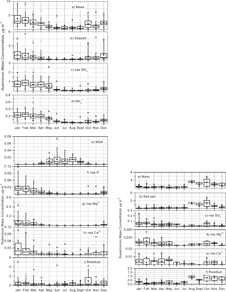
Figure 3. Box plots of submicron concentrations of (a)
gravimetrically determined aerosol mass, (b) sea salt, (c) nss
SO
4
=
, (d) NH
4
+
, (e) MSA
, (f) nss K
+
, (g) nss Mg
+2
, (h) nss
Ca
+2
, and (i) res idual mass as a function of month.
Percentile information is as in the Figure 1 caption.
Figure 4. Box plots of supermicron concentrations of (a)
gravimetrically determined aerosol ma ss, (b) sea salt, (c)
nss SO
4
=
, (d) nss Mg
+2
, (e) nss Ca
+2
, and (f) residual mass
as a function of month. Percentile information is as in the
Figure 1 caption.
QUINN ET AL.: CHEMICAL AND OPTICAL PROPERTIES AT BARROW, ALASKA AAC 8 - 7
regions. With no summer maximum, the Alert sea salt mean
concentrations are a factor of 10 to 18 lower than those
measured at Barrow.
[
32] Non-sea-salt SO
4
=
in the Arctic has several sources
[Ferek et al., 1995; Li et al., 1993; Barrie et al. , 1981].
Marine biogenic nss SO
4
=
is derived from the oxidation of
atmospheric dimethylsulfide (DMS) which, in turn, results
from oceanic phytoplankton processes. Anthropogenic sour-
ces incl ude the bu rning of fossil fuels and smelting of
sulfide ores in Eurasia.
[
33] Submicron nss SO
4
=
concentrations at Barrow begin
to increase in December and have a broad peak from
January to May (Figure 3c and Table 2). They drop off
sharply in June and remain low through November.
Several factors may contribute to the broad January to
May peak including the long-range transport of anthropo-
genic primary nss SO
4
=
, the long-range transport of anthro-
pogenic SO
2
that is then photooxidized to nss SO
4
=
, and
local production of biogenic nss SO
4
=
from the oxidation
of DMS. Barrie and Hoff [1984] attributed the March to
April peak in nss SO
4
=
observed in the Canadian Arctic to
the enhanced photooxidation of SO
2
to nss SO
4
=
as light
levels increase. Ferek et al. [1995] reported the presence
of DMS in Arctic waters under the ice as early as April
and suggested that as the ice recedes this DMS may be
converted to nss SO
4
=
and contribute to late spring con-
centrations. Elevated nss SO
4
=
concentrations in May
coincide with an increase in M SA concentrations
(Figure 3e), a species of pure biogenic origin. Hence a
biogenic source may contribute to the elevated nss SO
4
=
concentrations observed in May.
[
34] A linear regression of nss SO
4
=
concentrations versus
the aerosol light absorption coefficient, s
ap
, yields the
highest coefficient of determination, r
2
, for January (0.7)
and February (0.8) and lower values for December (0.4),
March (0.4), and April (0.47). Lowest values (0.03 to 0.21)
are obtained for May through November. Elevated levels of
s
ap
at a wavelength of 550 nm indicate the presence of
anthropogenic aerosol most likely in t he form of soot from
fossil fuel and biomass combustion. The regression results
suggest that nss SO
4
=
and s
ap
are derived from the same
source region during January and February but have differ-
ent sources (perhaps in addition to a common source)
during December, March, and April.
[
35] Supermicron nss SO
4
=
concentrations are about an
order of magnitude lower than submicron concentrations
(Figure 4c and Table 3). There is a seasonal trend of highest
mean concentrations in January and February, lower con-
centrations in March through June, and, with the exception
of October, lowest concentrations in July through December.
[
36] When using the SO
4
=
to Na
+
mass ratio for seawater
of 0.252 to calculate supermicron nss SO
4
=
concentrations,
Table 3. Supermicron Mass Concentrations at Barrow, Alaska, for October 1997 to December 2000
a
mgm
3
Mass Sea Salt nss SO
4
=
NH
4
+
MSA
nss Mg
+2
nss Ca
+2
Residual
b
Jan. 0.87 ± 0.55 0.32 ± 0.28 0.08 ± 0.08 0.006 ± 0.003 <0.0001 0.009 ± 0.007 0.004 ± 0.006 0.32 ± 0.19
Feb. 0.63 ± 0.67 0.28 ± 0.39 0.06 ± 0.03 0.007 ± 0.004 <0.0001 0.01 ± 0.01 0.003 ± 0.004 0.18 ± 0.20
March 0.72 ± 0.60 0.33 ± 0.44 0.05 ± 0.04 0.006 ± 0.005 <0.0001 0.007 ± 0.006 0.004 ± 0.004 0.13 ± 0.10
April 0.64 ± 0.31 0.29 ± 0.23 0.04 ± 0.03 0.004 ± 0.004 0.0001 ± 0.0002 0.006 ± 0.007 0.004 ± 0.005 0.24 ± 0.18
May 0.51 ± 0.58 0.34 ± 0.35 0.04 ± 0.02 0.003 ± 0.005 0.0004 ± 0.0005 0.005 ± 0.005 0.005 ± 0.003 0.21 ± 0.18
June 0.43 ± 0.39 0.26 ± 0.35 0.04 ± 0.01 0.003 ± 0.004 0.0007 ± 0.0007 0.001 ± 0.0004 0.002 ± 0.002 0.11 ± 0.07
July 0.82 ± 0.78 0.55 ± 0.62 0.01 ± 0.01 0.0004 ± 0.0005 0.0005 ± 0.0005 0.0005 ± 0.001 0.001 ± 0.002 0.23 ± 0.14
Aug. 3.1 ± 0.49 2.0 ± 0.33 0.01 ± 0.01 0.002 ± 0.002 0.001 ± 0.001 0.002 ± 0.003 0.001 ± 0.001 0.87 ± 0.17
Sept. 1.9 ± 0.92 1.4 ± 0.69 0.01 ± 0.01 0.0005 ± 0.0005 0.0008 ± 0.0008 0.003 ± 0.003 <0.0001 0.43 ± 0.24
Oct. 2.9 ± 1.9 2.1 ± 1.4 0.04 ± 0.04 0.0006 ± 0.001 <0.0001 0.006 ± 0.007 0.002 ± 0.004 0.82 ± 0.41
Nov. 2.0 ± 0.78 1.0 ± 0.67 0.02 ± 0.03 0.0006 ± 0.001 <0.0001 0.006 ± 0.004 0.002 ± 0.002 0.82 ± 0.50
Dec. 1.5 ± 0.89 0.69 ± 0.41 0.01 ± 0.01 0.002 ± 0.003 <0.0001 0.002 ± 0.002 0.001 ± 0.001 0.57 ± 0.33
a
Concentrations are reported as arithmetic mean and standard deviation (1s)at0C and 1013 mbar.
b
Calculated from the gravimetric mass less the ionic mass and associated water.
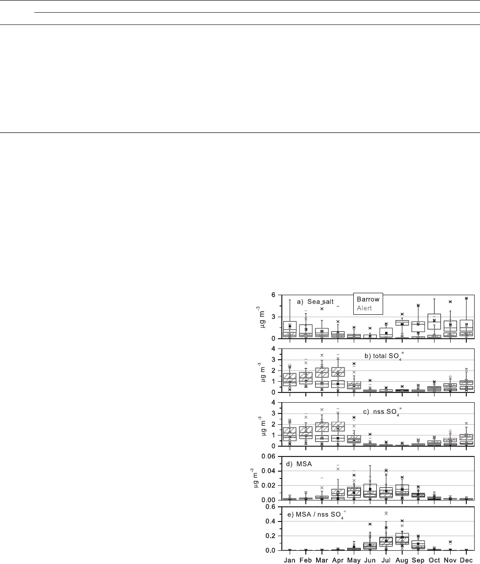
Figure 5. Box plots of total (submicron and supermicron)
concentrations of (a) sea salt, (b) total SO
4
=
, (c) nss SO
4
=
,
(d) MSA
, and (e) MSA
to nss SO
4
=
ratio from Barrow
(black line) and Alert (hatched boxes) as a function of
month. The Barrow data cover the period from October
1997 to December 2000, and the Alert data cover the period
from July 1980 to May 1995. Percentile information is as in
the Figure 1 caption.
AAC 8 - 8 QUINN ET AL.: CHEMICAL AND OPTICAL PROPERTIES AT BARROW, ALASKA
31% of the samples have negative nss SO
4
=
concentrations.
Negative nss SO
4
=
concentrations have also been reported
for firn samples from near the Antarctic ice edge [Gjessing,
1984] and at several coastal Antarctic stations [Wagenbach
et al., 1988, 1998] and have been attributed to sea salt
sulfate depletion. It has been hypothesized that sea salt
sulfate depletion is driven by the crystallization of mirabilite
(Na
2
SO
4
10H
2
O) [Richardson, 1976; Wagenbach et al.,
1998]. Mirabilite is associated with the ice lattice. The
remaining brine, which is not associated with the ice lattice,
becomes depleted in SO
4
=
at temperatures below 8.2C. It
is not known, however, how the brine becomes preferen-
tially airborne to form sea salt aerosol. With this process,
sea salt particles directly emitted from ice-free seawater will
not be fractionated.
[
37] The negative nss SO
4
=
concentrations derived from
using a seawater SO
4
=
to Na
+
ratio of 0.252 indicate that sea
salt sulfate may also be depleted at Barrow in the super-
micron size range. The degree of depletion is greatest for the
winter and spring (see section 2). It is within experimental
uncertainty for the summer season. The lack of a strong
depletion in summer is consistent with the brine/sea ice
hypothesis.
[
38] Seasonal cycles of total measured SO
4
=
and nss SO
4
=
for the sum of the submicron and supermicron size ranges
are similar at Barrow and Alert (Figures 5b and 5c). At both
stations, total and nss SO
4
=
concentrations are lowest from
June through September and increase steadily from October
through February. In March and April, concentrations at
Alert continue to increase, while they drop from the
February values at Barrow. Mean concentrations are similar
for May. The divergence of the seasonal cycles in March
and April may be a result of different transport patterns of
anthropogenic sulfate to Barrow and Alert and/or differ-
ences in the conversion processes of SO
2
to SO
4
=
either at or
en route to the two stations. A long-term trend in sulfate
may also be responsible in part since the Alert measure-
ments cover the period of 1980 to 1995 and the Barrow
measurements cover 1997 to 2000. Sirois and Barrie [1999]
report a decrease in sulfate in the winter/spring months at
Alert between 1991 and 1995. If this decrease is an Arctic-
wide phenomenon that has persisted through 2000, it may
account for some of the difference between the Alert and
Barrow March/April sulfate concentrations. However,
measurements of aerosol light scattering at Barrow give
no indication of a decrease between 1991 and 1995.
Scattering decreased between 1982 and 1992 [Bodhaine
and Dutton, 1993 ] but has leveled off since then. In
addition, sulfate measured during the three winter/spring
seasons between 1997 and 2000 gives no indication of a
decreasing trend at Barrow.
[
39] Particulate NH
4
+
results from the reaction of gas
phase NH
3
with acidic sulfate aerosol or other particulate
anionic species. NH
3
has both natural and anthropogenic
sources [Prospero et al., 1996]. Natural sources include
excreta from wild animals and emissions from soils, vege-
tation, and the ocean. Anthropogenic sources include fertil-
izer production and application, biomass burning, and
excreta from domestic animals.
[
40] The submicron NH
4
+
seasonal cycle at Barrow fol-
lows that of nss SO
4
=
with an increase in concentr ation in
December and a broad peak from January through May
(Figure 3d). Concentrations drop off sharply in June and
remain at their lowest levels through November. The
similarity in the behavior of NH
4
+
and nss SO
4
=
is most
likely a result of the fast reaction of NH
3
with acidic sulfate
aerosol near source regions outside of the Arctic. Mean
monthly NH
4
+
to nss SO
4
=
molar ratios fall within a relatively
narrow range of 1.5 to 1.75 for the wi nter and spring
seasons indicating a molecular composition between ammo-
nium bisulfate and ammonium sulfate. Mean ratios were
lower (1.1 to 1.4) for the summer months indicating less
availability of NH
4
+
to neutralize the sulfate aerosol. Super-
micron NH
4
+
concentrations were more than an order of
magnitude lower than the submicron concentrations
(Table 3) and made up, on average, less than 1 ± 1.4% of
the supermicron mass.
[
41] Atmospheric methans ulfonic acid or MSA
is
derived solely from the oxidation of biogenically produced
DMS. The seasonal cycle of submicron MSA
is out of
phase relative to the other chemical species measured.
Submicron concentrations begin to increase in April, peak
in May through September, and drop sharply in October
(Figure 3e and Table 2). Supermicron MSA
shows the same
seasonal behavior but only makes up 4 to 10% of the
summed submic ron and supermicron concentrations for
those months in which it is detectable (May through October)
(Table 3).
[
42] The late spring elevated MSA
concentrations
may be a result of long-range transport from oceanic
source regions in the North Pacific [Li et al., 1993]. By
late June, as the ice recedes in the Arctic and Bering
Seas, phytoplankton productivity in surface waters begins,
and DMS that is trapped under the ice is released. As the
ice melt continues, the Arctic Ocean can become a
substantial source of DMS through open leads and open
ocean waters [Ferek et al., 1995]. Ferek et al. [1995]
measured atmospheric DMS concentrations at Barrow
from M ay 31 to October 22, 199 1, and found that
concentrations were a few pptv in June, somewhat higher
in July, and reached a maximum near 100 pptv in the
middle of August before declining i n early fall. In
addition, Levasseur et al. [1994] suggested that DMS
released by ice algae during the ice breakup may con-
tribute to the early summer peak in DMS.
[
43] Barrow and Alert seasonal cycles of MSA
concen-
trations are compared in Figure 5d. They are similar in that
both show a maximum in spring and summer. The cycles
are slightly offset, however. Concentrations at Alert increase
in March, peak in May, and show a second peak in July. The
initial i ncrease at Barrow starts a month later (April)
followed by peaks in Jun e and August. Monthly mean
Barrow and Alert concentrations between May and Sep-
tember are within ±60%. MSA
to nss SO
4
=
ratios have
been used to determine the fraction of nss SO
4
=
that is
biogenically produced [e.g., Bates et al., 1992; Li et al.,
1993; Huebert et al., 1996]. Monthly mean MSA
to nss
SO
4
=
ratios during the first MSA
peak at Alert and Barrow
are 0.02 ± 0.02 and 0.08 ± 0.09 (arithmetic means and 1s
standard deviation), respectively (Figure 5e). During the
second peak, which occurs in the summer when anthropo-
genic nss SO
4
=
concentrations are expected to be lower,
monthly mean ratios are 0.17 ± 0.19 and 0.18 ± 0.08 at
Alert and Barrow, respectively.
QUINN ET AL.: CHEMICAL AND OPTICAL PROPERTIES AT BARROW, ALASKA AAC 8 - 9

[44] The particle number concentration at Barrow shows
a maximum in the summer months of June through
September [Polissar et al., 1999] (Figure 6e). During this
time period the submicron aerosol light scattering coeffi-
cient is relatively low (Figure 6a), indicating that the
increase in number concentration is due to small particles
which are inefficient scatterers of light. It has be en
hypothesized that the summer maximum in particle con-
centration is related to the formation of biogenic sulfur
particles [e.g., Bodhaine,1989;Polissar et al., 1999].
Measurements of vertical profiles of Aitken nucleus con-
centrations (diameters < 0.1 mm) and the light scattering
coefficient west of Barrow during June of 1990 support this
hypothesis [Ferek et al., 1995]. Two flights during haze-
free periods of moderate DMS concentration revealed high
concentrations of Aitken nuclei between 0.5 and 2 km near
the edges of stratus cloud layers from which snow was
falling. Measurements of the light scattering coefficient
showed no response to the high concentrations of Aitken
nuclei, confirming the presence of small particles. Ferek et
al. [1995] suggest that scavenging by the summertime low-
level stratus clouds removes accumulation mode aerosol.
The combination of low aerosol surface area and abundant
biogenic aerosol precursor (DMS) leads to particle produc-
tion thus influencing the particle number concentration
aloft and at the surface.
[
45] To further test the hypothesis, a linear regression of
submicron MSA
versus particle concentration was per-
formed for the months with detectable MSA
at Barrow.
The resulting r
2
was 0.8 indicating a strong correlation
between numb er concentration and biogenically derive d
aerosol mass.
[
46] Non-sea-salt K
+
in submicron particles is a useful
tracer of aerosol derived from biomass burning [e.g.,
Andreae , 1983; Gaudichet et al. , 1995]. Submicron nss
K
+
concentrations at Barrow begin to increase in December,
peak in January, and drop off from February through April
(Figure 3f and Table 2). Lowest concentrations are observed
in May to November. Hence nss K
+
follows the pattern of
other species that are transported long distances during the
winter/spring haze season. A linear regression of submicron
nss K
+
versus nss SO
4
=
results in a poor correlation (r
2
= 0.2),
however, confirming that they are derived from different
sources; nss SO
4
=
is primarily a product of fossil fuel
combustion and smelting of sulfide ores during this time
of year [Barrie et al., 1981], while nss K
+
results from
biomass burning.
[
47] Monthly mean supermicron nss K
+
concentrations
range between 0.003 and 0.006 mgm
3
. They are of the
same order of magnitude as summertime submicron con-
centrations but make up less than 0.3 ± 0.3% of the
supermicron mass.
[
48] Seasonal cycles of submicron nss Mg
+2
and Ca
+2
are shown in Figures 4g and 4h. Monthly mean concen-
trations of both ions are highest from December to March
suggesting long-range transport from Eurasia. Barrie and
Barrie [1990] attributed the presence of Mg and Ca in
Alert aerosol to windblown soil. Soil dust from Asia has
been observed in haze layers over Alaska [Rahn et al.,
1977] and the North Pacific [Uematsu et al., 1985] during
the springtime. Elevated aerosol Ca concentrations meas-
ured in the Norwegian Arctic during a March 1983
episode of long-range transport of poll utants from the
former Soviet Union were attributed to metal emissions
from coal combustion [Pacyna and Ottar, 1989]. Measure-
ments of other trace elements found in soil dust (Al, Si, Ti,
and Fe) would help to determine sources of the winter/
spring ma ximum in nss Mg
+2
and Ca
+2
measured at
Barrow. Low concentrations during the summer months
indicate there is no strong local source of submicron nss
Mg
+2
and Ca
+2
at Barrow.
[
49] Supermicron nss Mg
+2
concentrations peak in Jan-
uary through May and again in September through Novem-
ber (Figure 4d and Table 3). Supermicron nss Ca
+2
concentrations exhibit a similar double-peaked annual cycle
(Figure 4e and Table 3). This behavior suggests a distant
source in the winter/spring months and a local source in the
summer months. Barrie and Barrie [1990] reported a
similar two-peaked annual cycle in soil dust (represented
by Al) at Alert. Since the September soil dust peak does not
coincide with elevated dust concentrations from northern
hemisphere dust storms, they attributed it to the onset of
snow on the ground and the resuspension of soil promoted
by snow drifting over relatively bare soil.
5. Results: Seasonal Cycle of Optical Properties
and Relationship to Chemical Compositions
[50] The magnitude of the scattering coefficient of a
chemical component depends on its size-dependent mass
(or volume) concentration. For a wavelength of 550 nm,
Figure 6. Box plots of submicron aerosol (a) scattering
coefficient at 550 nm, (b) A
˚
ngstro¨m exponent for the 450
and 700 nm wavelength pair, (c) absorption coefficient at
550 nm, (d) single scattering albedo at 550 nm, and (e) the
particle number concentration. Percentile information is as
in the Figure 1 caption.
AAC 8 - 10 QUINN ET AL.: CHEMICAL AND OPTICAL PROPERTIES AT BARROW, ALASKA
particles of unit volume, and a refractive index of 1.5– 10
7
i,
which is near that of (NH
4
)
2
SO
4
and sea salt at low RH, the
scattering efficiency is lognormally distributed with the most
efficient size range for scattering occurring between particle
diameters of 0.2 and 1.0 mm[Quinn et al., 1996]. In addition,
it is the submicron particles that are transported over long
distances as deposition rates incr ease with particle size.
Therefore the discussion of aerosol optical properties meas-
ured at Barrow focuses on the submicron size range.
[
51] The seasonal cycle of s
sp
at Barrow has been
described previously by Bodhaine [1989] (for measure-
ments from 1976 to 1986) and Bodhaine and Dutton
[1993] (for measurements from 1976 to 1993). T hese
measurements were made on non-size- segregated aerosol
and therefore did not consider the submicron and super-
micron size ranges separately. This long-term record shows
maximum values of s
sp
in March and April that drop off in
May and reach the lowest values of the year in June.
Bodhaine [1989] also comment on episodic events of high
s
sp
and low A
˚
ngstro¨m exponents (indicating a relatively
large-sized aerosol) in October and November and hypothe-
size that these could be caused by sea salt or windblown
dust.
[
52] The seasonal cycle in submicron s
sp
measured since
October of 1997 (when the aerosol sampling system was
changed at Barrow to include a high-sensitivity nephelometer
sampling size-segregated aerosol at a reference RH) is similar
to that reported by Bodhaine [1989] and Bodhaine and
Dutton [1993] for the bulk aerosol. Scattering by submicron
aerosol begins to increase in October, is highest in December
through April, decreases in May, and drops to lowest levels in
June through September (Figure 6a). This trend follows the
combined trends of submicron sea salt and nss SO
4
=
, the two
dominant ionic aerosol chemical components at Barrow. A
linear regression of s
sp
(550nm) against sea salt mass con-
centrations for the months of October through January, the
period of high sea salt and relatively low nss SO
4
=
concen-
trations, results in a coefficient of determination, r
2
, of 0.64
(Figure 7a). On the basis of this analysis, sea salt can explain
about 60% of the variance in scattering for the submicron size
range for this period of the year. The October through January
regression for s
sp
(550 nm) versus nss SO
4
=
results in r
2
of
0.08 (Figure 7d). The correlation between measured s
sp
and
sea salt concentrations confirms the hypothesis of Bodhaine
[1989] that sea salt influences light scattering during October
and November.
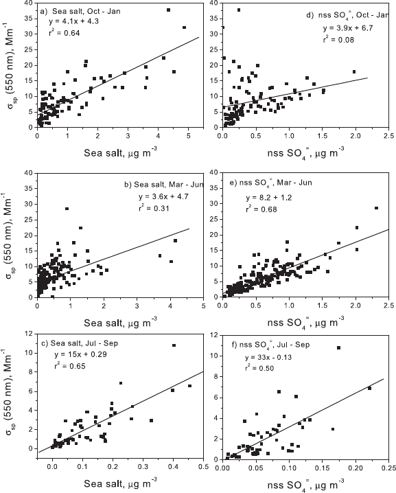
Figure 7. Linear regression of the mass concentrations of submicron sea salt or nss SO
4
=
versus
submicron s
sp
(550 nm) for the winter, spring, and summer seasons. Sea salt versus s
sp
(550 nm) is shown
for (a) October to January, (b) March to June, and (c) July to September. Non-sea-salt SO
4
=
versus s
sp
(550
nm) is shown for (d) October to January, (e) March to June, and (f ) July to September.
QUINN ET AL.: CHEMICAL AND OPTICAL PROPERTIES AT BARROW, ALASKA AAC 8 - 11
[53] Concentrations of submicron nss SO
4
=
are compara-
ble to those of submicron sea salt in March and higher than
those of sea salt in April, May, and June. A linear regression
of submicron s
sp
(550) versus nss SO
4
=
for March through
June results in an r
2
equal to 0.68 indicating that nss SO
4
=
can explain about 70% of the variance during the spring
(Figure 7c). The March through June regression for sea salt
yields an r
2
= 0.31 (Figure 7b).
[
54] Submicron mass concentrations are lowest in July
through September. During this summer period both sea salt
and nss SO
4
=
appear to contribute to s
sp
(550 nm). The value
of r
2
for s
sp
(550 nm) versus sea salt is 0.65 (Figure 7c) and
for nss SO
4
=
is 0.50 (Figure 7f).
[
55] On the basis of these results, for the submicron size
range, sea salt has a dominant role in controlling s
sp
(550
nm) in the winter, nss SO
4
=
is dominant in the spring, and
both components contribute to s
sp
(550 nm) in the summer.
[
56] The A
˚
ngstro¨m exponent, a˚, for the 450 and 700 nm
nephelometer wavelength pair was calculated from
a
¼
log
s
sp
450ðÞ
=
s
sp
700ðÞ
log
450
=
700
: ð2Þ
Similar to what was reported by Bodhaine [1989], there
is an increase in a˚ from January to June (Figure 6b)
indicating a shift in the aerosol population to relatively
smaller particles. Bodhaine [1989] attributed this increase
to more efficient gas-to-particle conversion during trans-
port from lower latitudes as the solar elevation increases.
Values remain high for the months of June through
August which corresponds to the time of year of lowest
aerosol mass concentrations and scattering coefficients
and highest MSA
and particle number concentrations.
The simultaneous occurrence of relatively small diameter
particles and high MSA
and particle number concentra-
tions further confirms that these particles are a result of
local biogenic origin.
[
57] The lower values of a˚ during the months of October
to January indicate a popu lation of relatively larger sub-
micron particles. On the basis of the chemical analysis these
larger diameter particles are most likely due to the influx of
sea salt to Barrow from the northern Pacific Ocean.
[
58] In general, the seasonal cycle of the submicron
absorption coefficient, s
ap
(550), follows that of the scatter-
ing coe fficient ( Figure 6c). (A linear reg ression of the
monthly arithmetic mean scattering versus absorption coef-
ficient yields an r
2
of 0.88.) There are differences between
the two seasonal cycles, however, that affect the seasonal
cycle of single scattering albedo. The mean absorption
coefficient peaks in February, while s
sp
(550 nm) peaks in
January to February. In addition, the annual cycle of s
ap
(550
nm) is stronger than s
sp
(550 nm). This difference most
likely is a result of the low frequency of long-range trans-
port of anthropog enic absorbing aerosol to the site in
summer alon g with a summertime source of biogenic
scattering aerosol. Hence the absorption coefficient appears
to be the less ambiguous marker for imported pollution.
[
59] Monthly percentile information for the aerosol single
scattering albedo, defined as
w ¼ s
sp
s
sp
þ s
ap
; ð3Þ
is shown in Figure 6d. Values of w are lowest in the winter
and spring (December through April) with a minimum value
in February (0.91 ± 0.04, arithmetic mean and 1s standard
deviation) corresponding to the peak in s
ap
. Values begin to
Table 4. Submicron Mass Scattering Efficiencies for the Dominant Aerosol Components (nss SO
4
=
and Sea Salt), the Residual Mass, and
the Total Submicron Aerosol
a
Season Number of Samples a
sp,SO4,ion,
m
2
g
1
a
sp,seasalt,
m
2
g
1
a
sp,res,
m
2
g
1
a
sp,sub,aer,
m
2
g
1
Oct. – Jan. 69 5.8 ± 1.0 1.8 ± 0.37 1.3 ± 0.63 2.4 ± 0.15
March – June 124 5.6 ± 0.32 2.9 ± 0.26 0.21 ± 0.31 2.9 ± 0.20
July – Sept. 40 4.1 ± 2.9 5.1 ± 0.97 1.5 ± 1.0 3.7 ± 0.49
All year 289 5.3 ± 0.28 2.2 ± 0.15 0.82 ± 0.26 2.5 ± 0.09
a
Values are reported at 33% RH and given as average plus or minus standard error.
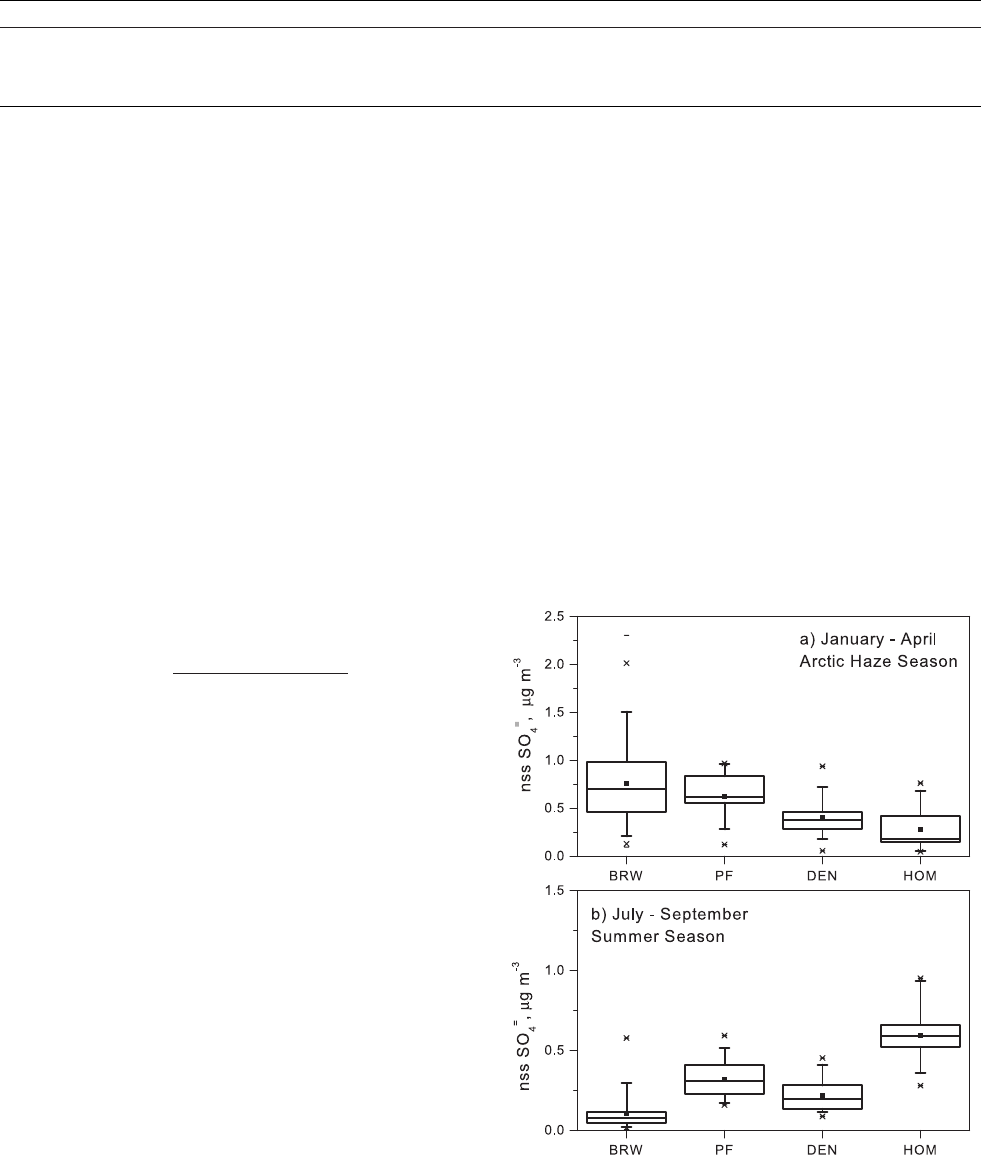
Figure 8. Comparison of nss SO
4
=
concentrations from
October 1997 to December 1999 measured at Barrow
(BRW), Poker Flat Rocket Range (PF), Denali National
Park (DEN), and Homer (HOM). Shown are data from the
(a) winter/spring haze season (January to April) and (b)
summer (July to September). Percentile information is as in
the Figure 1 caption.
AAC 8 - 12 QUINN ET AL.: CHEMICAL AND OPTICAL PROPERTIES AT BARROW, ALASKA
increase in May, reach a maximum in August (0.98 ± 0.02),
and then steadily decrease through December. The summer
maximum results from the lack of a source of summertime
absorbing aerosol.
[
60] The mass scattering efficiency of a chemical compo-
nent links the mass concentration of that component to its
light scattering efficiency. It is an essential quantity for
calculating its direct climate forcing [Charlson et al., 1999].
Mass scattering efficiencies for individual aerosol chemical
components can be estimated from a multiple linear regres-
sion of the mass concentration of each aerosol component
against the scattering coefficient for the whole aerosol. An
equation of t he following form, including only the major
aerosol components, was used to obtain weighted averages
of the submicron mass scattering efficiencies:
a
sp
¼ a
sp;seasalt
m
seasalt
þ a
sp;SO4;ion
m
SO4;ion
þ a
sp;res
m
res
; ð4Þ
where s
sp
is the measured submicron value, a
sp, j
is the
submicron mass scattering efficiency of component j, and
m
j
is the submicron mass concentration of component j
which, for sea salt and sulfate, includes associated water at
the measurement RH. In addition, the mass scattering
efficiency of the total submicron aerosol, a
sp,sub,aer
was
calculated from a linear regression of the submicron mass
concentration versus the submicron measured s
sp
. Calcula-
tions were done for the entire year, winter (October to
January), spring (March to June), and summer (July to
September). Resulting mass scattering efficiencies ar e
reported in Table 4.
[
61] Average values of a
sp,SO4,ion
were relatively constant
over all seasons with weighted averages ranging from 4.1 ±
2.9 to 5.8 ± 1.0 m
2
g
1
. The consistency of the values most
likely is a result of the stability in the nss SO
4
=
size dis-
tribution over the course of a year. Values of a
sp,seasalt
and
a
sp,res
vary more with season indicating a more variable size
distribution. The relatively large values of a
sp,seasalt
for the
months of July through September suggest that more coarse
mode sea salt mass extends in the optically efficient size
range (0.2 to 1.0 mm) during this time of year. Thi s is
consistent with a local source of sea salt such that the aerosol
is not transported over long distances with a loss of large
particle mass through deposition processes. The mass scat-
tering efficiencies for nss SO
4
=
ion and sea salt calculated for
the Barrow aerosol fall within the range of those determined
for t he central Pacific Ocean atmosphere [Quinn et al.,
1996]. In addition, the Barrow a
sp,SO4,ion
fall within the
theoretical range of low RH sulfate scattering efficiencies
predicted by Charlson et al. [1999].
6. Results: Comparison of Aerosol Chemical
Composition From Four Alaskan Sites
[62] Three sites in addition to Barrow form the Alaskan
aerosol sampling network. These are located, from north to
south, at Poker Flat Rocket Range (65.1N , 147.5W),
Denali National Pa rk (63.45N, 149.3W), and Homer
(59.7N, 151.5W). Using high-volume, non-size-segre-
gated samplers, weekly samples have been collected at
Poker Flat and Homer since 1995 and at Denali since
1997. The data from these sites are compared to those from
Barrow to determine how far south Arctic Haze extend ed
during the 1997/1998 and 1998/1999 haze seasons.
[
63] Data were divided into the haze season (January to
April) when nss SO
4
=
concentrations are highest and
anthropogenic influences are greatest and the summer
season (July to September) when nss SO
4
=
concentrations
are lowest. Percentile information for nss SO
4
=
concentra-
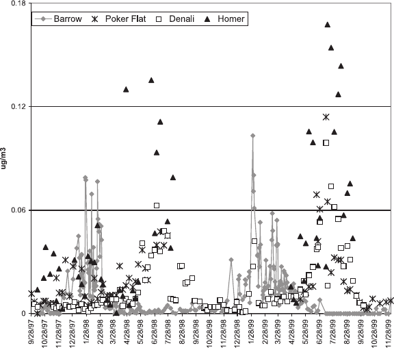
Figure 9. Non-sea-salt K
+
for October 1997 to December 1999 at Barrow, Poker Flat, Denali Nationa l
Park, and Homer.
QUINN ET AL.: CHEMICAL AND OPTICAL PROPERTIES AT BARROW, ALASKA AAC 8 - 13
tions for the four sites are shown in Figure 8. During the
haze season, concentrations are highest at Barrow and
decrease with latitude from Poker Flat to Denali to Homer.
The Brooks Range runs east-west south of Barrow and is
north of all of the other sites. It serves as a barrier to
transport o f aerosol to southern latitudes and is one
explanation for why winter/spring concentrations of nss
SO
4
=
are highest at Barrow. A second mountain range, the
Alaska Range, runs east-west north of Homer further
isolating this southernmost site from the impact of Arctic
Haze. As a result, concentrations of nss SO
4
=
are the lowest
here of the four sites during the haze season. Polissar et al.
[1998], assuming all measured elemental sulfur was due to
SO
4
=
, reported a similar gradient in maximum nss SO
4
=
concentration from northwest to southeast Alaska during
the winter and spring months.
[
64] In July through September, concentrations of nss
SO
4
=
are lowest at Barrow and highest at Homer. The source
of the summertime nss SO
4
=
at Homer may be biogenic from
DMS emissions in the Gulf of Alaska and Cooke Inlet. Past
and future samples collected at Homer will be analyzed for
MSA
to test this hypothesis.
[
65] Also compared were seasonal cycles of nss K
+
at the
four sites (Figure 9). As described in section 4.2, nss K
+
concentrations at Barrow peak in December through April
and are at a minimum in May through November following
the trend of other chemical species that make up the winter/
spring Arctic Haze. In contrast, nss K
+
concentrations at
Poker Flat, Denali, and Homer peak in the summer months
most likely due to local and/or regional forest fires. Polissar
et al. [1996] found a correlation between summer peaks of
aerosol optical absorption and fire activity for Gates of the
Arctic National Park and Denali during 1988, 1990, and
1991 and concluded that wood smoke from forest fires is
one of the most important regional sources of aerosol during
summer. On average, during the period from 1960 to 1997,
280,000 ha of boreal forest burned in Alaska each summer
with the peak in the fire season occurring in July and
August [Lavoue et al., 2000].
7. Conclusions
[66] Presented here are results from the longest reported
record of simultan eously measured aerosol chemical and
optical properties at Barrow, Alaska. Measurements have
been made since October of 1997 to present. Such simulta-
neous measurements allow for the identification of the
chemical components responsible for observed changes in
aerosol optical properties on seasonal, annual, and longer
timescales. Conti nuous measur ements of aeros ol ionic
chemical composition and light scattering indicate that sea
salt is dominant in controlling light scattering during winter,
nss SO
4
=
dominatesinspring,andbothplayarolein
summer. In addition, the mass fraction of residual (chemi-
cally unanalyzed) mass is equal to the ionic mass fraction
for the submicron size range in summer suggesting a role
for unidentified organic species in controlling aerosol light
scattering.
[
67] A strong correlation between MSA
and particle
number concentration during the summer indicates a source
of biogenic particles during this time of year. Low sub-
micron aerosol scattering coefficients and high A
˚
ngstro¨m
exponents indicate the presence of smaller diameter sub-
micron particles providing further evidence for this hypoth-
esis. It is likely that at least a portion of the summertime
residual mass also is of biogenic origin as there are no
strong anthropogenic sources of aerosol during this time of
year.
[
68] Mass scattering efficiencies of submicron nss SO
4
=
are relatively constant with season indicating a stable size
distribution throughout the year. Values for submicron sea
salt are more variable with season most likely due to
varying amounts of coarse mode sea salt tailing into the
submicron size range. Higher values occur during the
summer when supermicron sea salt concentrations are at a
maximum.
[
69] Non-sea-salt SO
4
=
concentrations during the haze
season (January through April) decrease with decreasing
latitude from Barrow south to Homer. Hence there appears
to be a latitudinal gradient in the extent of Arctic haze. In
con trast, nss SO
4
=
concentrations at Homer are highest
during the summer presumably due to a stronger biogenic
source. This needs to be confirmed with measurements of
MSA
concentrations, however.
[
70] Th e 3-year record of aerosol measurements pre-
sented here has allowed for the assessment of seasonal
changes in aerosol optical properties with respect to changes
in aerosol ionic composition. A longer data record is
needed, however, to determine longer-term trends in Arctic
Haze and to detect changes in aerosol sources and transport
pathways to the Arctic associated with climate change. In
addition, other questions remain including what the sub-
stantial submicron resi dual mass during the summer is
composed of. With more complete chemical analysis,
including routine measurements of organic carbon, black
carbon, and trace elements, it would be possible to address
this question and that of changing aerosol sources and
transport to the Arctic.
[71] Acknowledgments. We thank Dan Endres and Andrea Blakesley
for help in collecting samples at Barrow, Denali, Poker Flat, and Homer. We
thank Derek Coffman for performing the thermodyamic equilibrium model
calculations, Jim Johnson for the trajectory calculations, and Drew Ham-
ilton for logistical assistance. The Alert data were graciously provided by
Len Barrie and the Meteorological Service of Canada. This work was
supported by NOAA’s Arctic Program and NOAA’s Office of Global
Programs’ Aerosol Program. This is PMEL contribution 2367 and JISAO
contribution 853.
References
Anderson, T. L., and J. A. Ogren, Determining aerosol radiative properties
using the TSI 3563 integrating nephelometer, Aerosol Sci. Technol., 29,
57 – 69, 1998.
Andreae, M. O., Soot carbon and excess fine potassium: Long-range trans-
port of combustion-derived aerosols, Science, 220, 1148–1151, 1983.
Ayers, G. P., M. D. Keywood, and J. L. Gras, TEOM vs. manual gravi-
metric methods for determination of PM2.5 aerosol mass concentrations,
Atmos. Environ., 33, 3717 – 3721, 1999.
Barrie, L. A., and M. J. Barrie, Chemical components of lower tropospheric
aerosols in the high Arctic: Six years of observations, J. Atmos. Chem.,
11, 211– 226, 1990.
Barrie, L. A., and R. M. Hoff, The oxidation rate and residence time of
sulphur dioxide in the Arctic atmosphere, Atmos. Environ., 18, 2711 –
2722, 1984.
Barrie, L. A., R. M. Hoff, and S. M. Daggupaty, The influence of mid-
latitudinal pollution sources on haze in the Canadian Arctic, Atmos. En-
viron., 15, 1407 – 1419, 1981.
Barrie, L. A., M. P. Olson, and K. K. Oikawa, The flux of anthropogenic
sulphur into the Arctic from mid-latitudes in 1979/80, Atmos. Environ.,
23, 2505 – 2512, 1989.
AAC 8 - 14 QUINN ET AL.: CHEMICAL AND OPTICAL PROPERTIES AT BARROW, ALASKA
Bates, T. S., J. A. Calhoun, and P. K. Quinn, Variations in the concentration
ratio of methane-sulfonate to sulfate in marine aerosol particles over the
South Pacific Ocean, J. Geophys. Res., 97, 9859 – 9865, 1992.
Berner, A., C. Lurzer, F. Pohl, O. Preining, and P. Wagner, The size dis-
tribution of the urban aerosol in Vienna, Sci. Total Environ., 13, 245 –
261, 1979.
Bodhaine, B. A., Barrow surface aerosol: 1976 – 1986, Atmos. Environ., 23,
2357 – 2369, 1989.
Bodhaine, B. A., Aerosol absorption measurements at Barrow, Mauna Loa,
and the South Pole, J. Geophys. Res., 100, 8967 – 8975, 1995.
Bodhaine, B. A., and E. G. Dutton, A long-term decrease in Arctic haze at
Barrow, Alaska, Geophys. Res. Lett., 20, 947 – 950, 1993.
Bond, T. C., T. L. Anderson, and D. Campbell, Calibration and intercom-
parison of filter-based measurements of visible light absorption by aero-
sols, Aerosol Sci. Technol., 30, 582 – 600, 1999.
Bridgman, H. A., and B. A. Bodhaine, On the frequency of long-range
transport events at Point Barrow, Alaska, 1983– 1992, Atmos. Environ.,
28, 3537 – 3549, 1994.
Charlson, R. J., T. L. Anderson, and H. Rodhe, Direct climate forcing by
anthropogenic aerosols: Quantifying the link between atmospheric sulfate
and radiation, Contrib. Atmos. Phys., 72(1), 79 – 94, 1999.
Delene, D. J., and J. A. Ogren, Variability of aerosol optical properties at
four North American surface monitoring sites, J. Atmos. Sci., 59(6),
1135 – 1150, 2002.
Draxler, R. R., Hybrid Single-Particle Lagrangian Integrated Trajectories
(HY-SPLIT): Version 3.0. user’s guide and model description, Tech. Rep.
ERL ARL-195, Natl. Oceanic and Atmos. Admin., Silver Spring, Md.,
1992.
Ferek, R. J., P. V. Hobbs, L. F. Radke, J. A. Herring, W. T. Sturges, and
G. F. Cota, Dimethyl sulfide in the arctic atmosphere, J. Geophys. Res.,
100, 26,093 – 26,104, 1995.
Gaudichet, A., F. Echalar, B. Chatenet, J. P. Quisefit, G. Malingre, H.
Cachier, P. Buat-Menard, P. Artaxo, and W. Maenhaut, Trace elements
in tropical African savanna biomass burning aerosols, J. Atmos. Chem.,
22, 19 – 39, 1995.
Gjessing, Y., Marine and non-marine contribution to the chemical composi-
tion of snow at the Riiser-Larsen ice shelf in Antarctica, Atmos. Environ.,
23, 155 – 160, 1984.
Heintzenberg, J., and S. Larssen, SO
2
and SO
4
in the Arctic: Interpretation
of observations at three Norwegian Arctic-Subarctic stations, Tellus, Ser.
B, 35, 255 – 265, 1983.
Holland, H. D., The Chemistry of the Atmosphere and Oceans, p. 154, John
Wiley, New York, 1978.
Hopper, J. F., D. E. J. Worthy, L. A. Barrie, and N. B. A. Trivett, Atmo-
spheric observations of aerosol black c arbon, carbon dioxide, a nd
methane in the high Arctic, Atmos. Environ., 28, 3047 – 3054, 1994.
Huebert, B. J., D. J. Wylie, and J. A. Heath, Production and loss of metha-
nesulfonate and non-sea -salt sulfate in the equatorial Pacific marine
boundary layer, Geophys. Res. Lett., 23 , 737 – 740, 1996.
Iversen, T., and E. Joranger, Arctic air pollution and large-scale atmospheric
flows, Atmos. Environ., 19, 2099 – 2108, 1985.
Langner, J., and H. Rodhe, A global three-dimensional model of the tropo-
spheric sulfur cycle, J. Atmos. Chem., 13, 225 – 263, 1991.
Lavoue, D., C. Liousse, H. Cachier, B. J. Stocks, and J. G. Goldhammer,
Modeling of carbonaceous particles emitted by boreal and temperate wild
fires at northern latitudes, J. Geophys. Res., 105, 26,871 – 26,890, 2000.
Levasseur, M., M. Gosselin, and S. Michaud, A new source of dimethyl-
sulfide (DMS) for the arctic atmosphere: Ice diatoms, Mar. Biol., 121,
381 – 387, 1994.
Li, S. M., and J. W. Winchester, Geochemistry of organic and inorganic
ions of late winter Arctic aerosols, Atmos. Environ., 23, 2401 – 2415,
1989.
Li, S. M., L. A. Barrie, and A. Sirois, Biogenic sulfate aerosol in the Arctic
troposphere, 2, Trends and seasonal va riations, J. Geophys. Res., 98,
20,623 – 20,631, 1993.
Lowenthal, D. H., and K. A. Rahn, Regional sources of pollution aerosol at
Barrow, Alaska, during winter 1979 – 80 as deduced from elemental tra-
cers, Atmos. Environ., 19, 2011–2024, 1985.
Meyer, M., J. Lijek, and D. Ono, Continuous PM10 measurements in a
woodsmoke environment, in PM10 Standards and Nontraditional Parti-
culate Source Controls, edited by J. C. Chow and D. M. Ono, vol. 1,
Tech. Rep. TR-22, pp. 2 – 38, Air and Waste Manage. Assoc., Pittsburgh,
Pa., 1992.
Norman, A. L., L. A. Barrie, D. Toom-Sauntry, A. Sirois, H. R. Krouse,
S. M. Li, and S. Sharma, Sources of aerosol sulfate at Alert: Apportion-
ment using stable isotopes, J. Geophys., Res., 104, 11,619–11,631, 1999.
Pacyna, J. M., and B. Ottar, Origin of natural constituents in the Arctic
aerosol, Atmos. Environ., 23, 809 – 811, 1989.
Polissar, A. V., P. K. Hopke, W. C. Malm, and J. F. Sisler, The ratio of
aerosol optical absorption coefficients to sulfur concentrations as an in-
dicator of smoke from forest fires when sampling in polar regions, Atmos.
Environ., 30, 1147–1157, 1996.
Polissar, A. V., P. K. Hopke, W. C. Malm, and J. F. Sisler, Atmospheric
aerosol over Alaska, 1, Spatial and seasonal variability, J. Geophys. Res.,
103, 19,035 – 19,044, 1998.
Polissar, A. V., P. K. Hopke, P. Paatero, Y. J. Kaufmann, D. K. Hall, B. A.
Bodhaine, E. G. Dutton, and J. M. Harris, The aerosol at Barrow, Alaska:
Long-term trends and source locations, Atmos. Environ., 33, 2441 – 2458,
1999.
Prospero , J. M., K. Barrett, T. Church, F. Dentener, R. A. Duce, J. N.
Galloway, H. Levy, J. Moody, and P. Quinn, Atmospheric deposition
of nutrients to the North Atlantic Basin, Biogeochemistry, 35, 27 – 73,
1996.
Quinn, P. K., and D. J. Coffman, Local closure during ACE 1: Aerosol mass
concentration and scattering and backscattering coefficients, J. Geophys.
Res., 103, 16,575 – 16,596, 1998.
Quinn, P. K., V. N. Kapustin, T. S. Bates, and D. S. Covert, Chemical and
optical properties of marine boundary layer aerosol particles of the mid-
Pacific in relation to sources and meteorological transport, J. Geophys.
Res., 101, 6931 – 6951, 1996.
Quinn, P. K., D. J. Coffman, V. N. Kapustin, T. S. Bates, and D. S. Covert,
Aerosol optical properties in the marine boundary layer during ACE 1
and the underlying chemical and physical aerosol properties, J. Geophys.
Res., 103, 16,547 – 16,563, 1998.
Quinn, P. K., et al., Surface submicron aerosol chemical composition: What
fraction is not sulfate?, J. Geophys. Res., 105, 6785 – 6806, 2000.
Rahn, K. A., The Mn/V r atio as an indicator of la rge-scale sources of
pollution aerosol for the Arctic, Atmos. Environ., 15, 1457–1464, 1981a.
Rahn, K. A., Relative importances of North America and Eurasia as sources
of Arctic aerosol, Atmos. Environ., 15, 1447 – 1455, 1981b.
Rahn, K. A., R. D. Borys, and G. E. Shaw, The Asian source of Arctic haze
bands, Nature, 268, 713 – 715, 1977.
Richardson, C., Phase relationship in sea ice as function of temperatures,
J. Glaciol., 17, 507 – 519, 1976.
Schnell, R. C., T. B. Watson, and B. A. Bodhaine, NOAA WP-3D instru-
mentation and flight operations on AGASP-II, J. Atmos. Chem., 9, 3–16,
1989.
Shaw, G. E., Eddy diffusion transport of Arctic pollution from the mid-
latitudes: A preliminary model, Atmos. Environ., 15, 1483–1490,
1981.
Sirois, A., and L. A. Barrie, Arctic lower tropospheric aerosol trends and
composition at Alert, Canada: 1980 – 1995, J. Geophys. Re s., 104,
11,599–11,618, 1999.
Sturges, W. T., and L. A. Barrie, Chlorine, bromine, and iodine in Arctic
aerosols, Atmos. Environ., 22, 1179–1194, 1988.
Uematsu, M., R. A. Duce, and J. M. Prospero, Deposition of atmospheric
mineral particles in the North Pacific Ocean, J. Atmos. Chem., 3, 123 –
128, 1985.
Wagenbach, D., U. Gorlach, and K. Moser, Coastal Antarctic aerosol: The
seasonal pattern of its chemical composition and radionuclide content,
Tellus, 40, 426 – 436, 1988.
Wagenbach, D., F. Ducroz, R. Mulvaney, L. Keck, A. Minikin, J. Legrand,
J. S. Hall, and E.W. Wolff, Sea-salt aerosol in coastal Antarctic regions,
J. Geophys. Res., 103, 10,961 – 10,974, 1998.
Watts, S. F., R. Yaaqub, T. Davies, D. H. Lowenthal, K. A. Rahn, R. M.
Harrison, B. T. Storr, and J. L. Baker, The use of Whatman 41 filter
papers for high-volume aerosol sampling, Atmos. Environ., 21, 2731 –
2736, 1987.
E. Andrews and J. A. Ogren, Climate Monitoring and Diagnostics
Laboratory, NOAA, 325 Broadway R/CMDL, Boulder, CO 80305, USA.
T. S. Bates, T. L. Miller, and P. K. Quinn, Pacific Marine Environmental
Laboratory, NOAA, 7600 Sand Point Way NE, Seattle, WA 98115-6349,
USA. ([email protected])
G. E. Shaw, Geophysical Institute, University of Alaska, Fairbanks, AK
99775, USA.
QUINN ET AL.: CHEMICAL AND OPTICAL PROPERTIES AT BARROW, ALASKA AAC 8 - 15
