The Great Housing Boom in China



Kaiji Chen

Yi Wen

February 16, 2014

Abstract

China’s decade-long housing boom looks nothing short of a gigantic bubble famil-

iar to many countries: In big cities the price-to-income ratio reached 30 to 1 and the

vacancy rate stood at 30% or above. This paper provides a theoretical framework to

shed light on the causes and consequences of the great housing boom in China. We

argue that the boom could be a rational bubble rooted in China’s unprecedented eco-

nomic transition— which features persistent high returns to capital. We argue that the

very expectation that China’s high capital returns driven by cheap labor and resource

relocations are not sustainable in the long run can induce investors to seek alternative

store of value for their growing wealth, thus triggering a self-ful…lling housing bubble in

a …nancially underdeveloped economy with limited supply of …nancial assets. The bub-

ble would exhibit a rapidly rising housing price-to-disposable income ratio during the

transition path regardless of whether housing provides rents or utilities. This predic-

tion is consistent with China’s “ghost town”phenomenon and decade-long faster-than-

income-growth housing bubble, which cannot be explained by standard neoclassical

growth theory. We show the bubble could prolong China’s economic transition and

severely reduce social welfare. Our model also sheds considerable light on similar hous-

ing bubbles existed in other emerging economies during their rapid economic growth

and transition periods.

Keywords: Housing Bubble, Capital Misallocation, Crowding-Out, Chinese Econ-

omy, Economic Transition.

JEL Codes: E22, E23, O16, O53, P23, P24, P31.



We thank Xiangyu Gong, Xin Wang and Tong Xu for capable research assistance and Jing Wu for

sharing data on China’s housing prices.

Economics Department, Emory University.

School of Economics and Management, Tsinghua University; and Research Department, Federal Reserve

Bank of St. Louis.

1 Introduction

Standard neoclassical theory suggests that housing (land) prices can grow at most as fast

as aggregate productivity under a …xed land supply. But this is not true in China. Housing

prices in China experienced rapid and steady accelerations far above productivity growth

since the housing reform in the late 1990s and, especially, in the recent decade. In many

cities, the growth of housing prices signi…cantly outpaced the growth of disposable income.

For example, data based on 35 major Chinese cities show that in most of these cities the

growth rate for real housing prices b etween 2006-2010 are between 15% to 30% per year, far

exceeding the 10% growth rate for real disposable income in these cities.

As a consequence,

the nation-wide average house price-to-income ratio increased from around 8 in 1999 to 13

in 2010, and this ratio reached about 30 in big cities such as Beijing and Shanghai, despite

unprecedented income growth. The increase in housing prices is also accompanied by rapidly

rising land values in China. Using data from the local land auction market in Beijing, Wu,

Gyourko, and Deng (2010) show that real constant quality land values have increased by

nearly 800% since the …rst quarter of 2003.

Because of the phenomenal rate of return in the housing market, real estate has become

a vital investment opportunity for households, state-owned enterprises, private …rms, as well

as commercial banks. So housing investors in China include people from all walks of life,

regardless of their income level and profession, and enterprises of all types, regardless of

their sizes and ownerships. In fact, capital gains from housing investment have become an

important (or even the only) source of pro…ts for many state-owned and private …rms. Given

the sheer size of China’s housing market (with a population of 1.3 billion and 230 millions

new migrants into cities in recent decade and a similar-size migration in the next decade)

and the long duration of the rapid housing-price growth, what we are witnessing can be truly

called one of the greatest housing booms in human history.

The astonishingly high price-to-income ratio seems to suggest excess demand in the

housing market; yet “ghost towns”and massive empty apartments across big cities in China

appear to indicate excess supply. As if this mismatch in demand and supply is not puzzling

enough, there exists even a bigger puzzle: housing prices keep growing rapidly in recent years

despite the alarmingly high vacancy ratio.

See Wu, Deng, and Liu (2012, Fi g. 5).

On the one hand, the great housing boom appears no di¤erent from a typical housing

bubble experienced by many countries, such as Japan in the 1970s and 80s and the United

States in the 2000s, except that the Chinese situation looks worse: The housing price-to-

income ratio in big Chinese cities is twice as high as in Japan when Japan’s housing bubble

burst in 1990, and six times as high as in the United States at the peak of the U.S. housing

bubble in 2005-2006. Vacancy rates in China are between 25% and 30%, well above the

normal range of 5 to 10 percent in advanced countries. On the other hand, the great housing

boom also looks unique to China: the ghost towns, ghost malls, and ghost apartments in

China make even the unprecedented Japanese bubble thirty years ago look pale.

Not surprisingly, the great housing boom in China has generated global attentions. The

fear is that the rapid housing price growth is not sustainable and a collapse of the Chinese

housing market may intensify the current world slump and signi…cantly prolong the world-

wide recession amidst of the world …nancial and debt crisis, given China’s increasing role as

an engine of global economic growth. The great housing boom has also caused great concerns

by the Chinese government, as excessive investment in housing can crowd out investment

in …xed capital and other real economic activities, and a sudden collapse of the bubble may

cause massive bank failures and jeopardize China’s economic growth potentials.

What economic forces are at work to generate the great housing boom in China? Are

the faster-than-income-growth housing boom sustainable? What are the economic costs of

the great housing boom?

Many conventional views exist to explain the great housing boom in China. One theory

views the boom as a natural consequence of China’s rapid income growth and rising urban

demand for housing. When total income grows rapidly but the supply of land is inelastic,

a growing demand for housing can easily push up housing prices. This theory predicts that

housing prices can grow as fast as aggregate income growth. Another view is that the housing

boom is a pure bubble because in …nancially underdeveloped economies houses can serve as

an attractive store of value even if they provide no utilities (as in the classical Samuelson

model of …at money). This view can explain the ghost-town phenomenon in China but

requires the additional assumption that the rate of return to capital (or interest rate) in

China is excessively low so that capital is not an idea asset to invest compared to housing.

But the rate of return to capital in China is not low: Its real rate of return has been above

20% per year over the past decades despite decades-long excessive investment (Bai, Hsieh

and Qian, 2006). Therefore, these conventional views cannot explain why the growth rate

of housing prices in China have remained so high for so long, far exceeding the growth rate

of aggregate disposable income despite the excessively high rate of return to capital.

This paper provides a theoretical framework to address these puzzles. We show that

the great housing boom in China can be a rational bubble arising naturally from China’s

unprecedented economic transition— which features phenomenal rates of return to capital

driven largely by newly emerging private …rms and massive relocations of cheap labor from

rural to urban areas, from po or to rich cities, and from SOEs (state-owned enterprises) to

private enterprises during the transition.

As unprecedented as it is, however, no rational investors would expect China’s growth

miracle to continue forever. The cheap labor resource may one day be exhausted; the high

return to capital may eventually come to an end; and the cheap credit supply due to …nancial

repression cannot possibly last forever. In deed, a recent survey of the biggest private …rms

in China shows that the top concerns for their future pro…tability are the rising costs in (i)

raw materials, (ii) labor, (iii) credit, and (iv) tax burdens. Thus, the rational anticipation of

increasing costs and declining capital returns in the future would motivate rational investors

to seek alternative stores of value beside capital.

Part of China’s rapid growth came from the government’s massive investment in in-

frastructures. As a result, China’s public debt has increased rapidly over the past decade.

The burden of repaying the debt will ultimately fall upon future generations. This antic-

ipation of rising corporate taxes further reinforces the public’s expectation of low future

after-tax capital returns in the private sector, further encouraging people to seek alternative

stores of value for their growing wealth.

Capital controls and an underdeveloped …nancial market in China (as is the case for many

developing countries) have limited the availability of stores of value for the rapidly increasing

wealth held by households and entrepreneurs; thus, investing in housing becomes one of the

best choices in China for capital gains.

We show that this expectation-drive strong demand

for housing as an alternative store of value, based on the foresight that China’s low-cost

and high-capital-return economy will eventually come to an end, can generate a large, fast-

growing, and self-ful…lling housing bubble at the present. That is, even if housing provides

no rents or utilities, rational agents would still hold it as a store of value if its rate of return

There is another puzzle the standard neoclassical model cannot explain: consumption-to-income ratio in

China has been declining over the past decades (see Wen, 2012). If housing provides utilities and its prices

grow faster than income, then as a normal good the consumption-to-income ratio should also increase over

time.

In China government tax income comes mainly from corporate taxes, instead of household income,

because of limited capacity in income-tax collection.

Laws in China prohibit people purchasing land as a store of value. Otherwise it may be more e¢ cient

to use land rather than vacant houses as a store of value.

(capital gain) equals or exceeds that of capital— which is exceptionally high during transition

but would surely be signi…cantly reduced after the transition ends. Consequently, a bubbly

equilibrium exists in which the growth rate of housing prices equals the rate of return to

capital. Hence, along the transition path we will observe a S-shaped housing price-to-income

ratio— with housing price growing much faster than disposable income in the initial stage of

the transition but eventually converging to the growth rate of disposable income in the long

run. This prediction appears consistent with the Chinese data.

We show that the housing bubble could greatly prolong China’s economic transition and

reduce social welfare. Unlike some existing bubble models, in our model housing bubbles

can exist without dynamic ine¢ ciency, due to the disparity between so cial and private rate

of returns to capital. Hence, by crowding out private capital formation and other productive

activities, it creates a negative externality and reduces the permanent income of all agents.

Accordingly, the occurrence of the housing bubble generates a substantial degree of resource

misallocation and welfare losses, prolonging economic transition and slowing down aggregate

economic growth.

Our model not only rationalizes the great housing boom in China, but also shed consid-

erable light on housing bubbles experienced in many emerging economies, such as the Asian

four tigers. These economies all exp erienced a transition period featuring low wage growth

and high capital returns sustained by labor relocations, and also su¤ered from underdevel-

oped …nancial markets and the lack of store of value for their growing wealth. Hence, with

currently high capital returns and anticipated low future capital returns, people opt to seek

alternative stores of value for their rapidly accumulated wealth. Given the capital control

policies widely adopted by governments to prevent capital out‡ows, land and housing stocks

become the natural choice of asset investment.

Our paper is related to several strands of the literature. First, our theory relies on a

similar mechanism as in Song, Storesletten and Zillibotti (2011, “SSZ”hereafter) to generate

a persistently high rate of return to capital along transition. Speci…cally, SSZ provide an over

lapping generations model with two sectors: one operates with ine¢ cient technology and the

other has superior technology but little access to bank capital, thus must rely on self …nance.

They show that labor relocation from the former to the latter sector can generate endogenous

productivity growth at the aggregate level, and account for China’s high income growth, high

capital returns, and large capital account surplus. In SSZ, however, investors’only portfolio

choice is between capital investment and bank deposit. As a result, their paper is silent on

why housing bubbles may occur in China, and thus unable to explain why the allocative

e¢ ciency in China can become worse as a result of the housing bubble— a phenomenon also

shared by other emerging economies in Asia. By introducing housing as a bubble asset into

the SSZ model, our paper not only sheds light on the formation of housing bubbles along

the economic transition, but also their social costs in terms of resource misallocation and

welfare. In particular, we explain why entrepreneurs in China have strong incentives to

own empty apartments that generate zero rents or utilities. By showing housing bubble as

a natural consequence of economic transition and studying what policies may correct the

consequent distortions, our paper complements SSZ in understanding the typical growth

pattern of emerging economies like China.

Our paper also contributes to the emerging literature on China’s housing price puzzle.

Most works in this area focus on why the housing price level is so high in China. For

example, Wei, Zhang and Liu (2011) provide a theory to link the high housing price level

in major cities of China to these areas’high household saving rates due to unbalanced sex-

ratio. In sharp contrast, the focus of our paper is on why housing prices in China have

grown faster than aggregate income over the last decade. To understand China’s growing

housing bubble, models that only explain high housing price level from the demand side are

not su¢ cient. More importantly, by shifting the analysis from housing price level to housing

price growth, our paper sheds light on why the rapid growth of housing prices may create

resource misallocation and prolong China’s economic transition, an issue silent in Wei et. al

(2011).

Our paper …ts into the fast-growing literature of economic development and resource

misallocation, with a focus on …nancial under-development.

We share the similar view that

…nancial under-development, especially …nancial repression, is key to resource misallocation

along transition. To our knowledge, we are the …rst to incorporate housing as a bubble

asset in this literature and analyze in detail its social and welfare costs in terms of economic

transition.

Finally, our theory is related to the existing theories on housing bubble. Tirole (1985)

and Farhi and Tirole (2011) emphasize the crowding-out e¤ects of bubble assets on capital

accumulation and its negative welfare e¤ects. On the other hand, Ventura (2012), Martin

and Ventura (2012), Caballero and Krishnamurthy (2006), and Kocherlakota (2009) show

that bubbles can crowd in capital accumulation when …rms are b orrowing constrained and

can use the bubble as collateral or a store of value to facilitate intertemporal consumption

smoothing. We show that even if the bubble asset can serve as collateral for borrowing, it

See, for example, Buera and Shin (2011) and Moll (2011).

can still crowd out capital formation and hinder welfare.

The remaining part of the paper is organized as follows: In Section 2, we present the

empirical facts about China’s growing housing bubble. Section 3 describes a simple 2-period

benchmark model to illustrate our essential …ndings. Section 4 reports the model’s simulation

results. In Section 5, we conduct a quantitative analysis based on a multi-period version of

our model. Section 6 concludes.

2 Empirical Facts

2.1 Chronology

China economic reform started in 1978. In the era of planned economy (b etween 1950 and

1978), all housing (apartments) in the city were provided by the government at subsidized

rents. All institutions, no matter whether they are hospitals, schools, or …rms, are obligated

to provide housing to their workers. This situation changed gradually since the reform.

In particular, from 1982 to 1985, more than 1,600 cities in China launched pilot projects of

housing reforms. Most of these projects focused on privatizing the existing public apartments

and let residents to pay the market-determined rents. However, due to the delay of wage

reforms and the lack of a …nancial system to provide loans, the …rst round housing reform

failed.

In 1991, the city of Shanghai built a system of publicly pooled funds for housing …nance.

This experiment was later introduced to the entire country between 1994 and 1997. The

pooled funds provided loans to enterprises and public institutions to build private housing

units and to individuals to purchase housing units— which was also the only channel for

individuals to obtain loans in those days. During this period, about 20% to 30% of the

existing housing stock was traded in the market, so the bulk of housing units was still

provided by the government at subsidized rates.

Things changed dramatically in 1998, in which year China’s State Council lunched a new

round of housing reform and issued “Notice on the Further Deepening of Urban Housing

Reform”(the 23rd Decree). After that, public housing provision essentially ended nationwide

and bank mortgage loans became available to home builders and home buyers in addition

to publicly pooled funds. Consequently, China entered an era of housing market boom. The

share of private housing units in total housing units increases from 30% to more than 70%

between 1998 and 2010.

2.2 Housing Prices and Disposable Income

The National Bureau of Statistics of China (NBSC) provides two major housing price indexes.

Based on these housing price indexes, the average growth rate of housing prices in China

is below the average growth rate of household disposable income. However, Wu, Deng,

and Liu (WDL 2012) argue that these measures are severely biased downward because they

include all existing houses in areas that are not yet included by market transactions or do not

have realistic market values. These authors instead use independently constructed housing

price index based on newly-built housing sales in 35 major Chinese cities. Their price index

demonstrates that the government-published data are severely downward biased and fail to

capture the dramatic increases in housing prices across the nation. Based on their data

set on newly-built housing sales, the average housing prices in China’s 35 major cities have

increased from a level of 100 in early 2004 to a level of 250 in late 2009, implying an average

annual growth rate of 17% per year. If we ignore the negative impact of the …nancial crisis,

the average growth rate was 20% p er year between 2004 and 2008 and this growth rate

become 25% in the year 2009 (see Panel A of Figure 1). In big cities the growth rate is even

higher. For example, in Shanghai and Beijing the average real growth rate of housing prices

during the same period is 2-3 times higher than the average real growth rate of disposable

income (see Figure 1B).

Yang, Chen, and Monarch (YCM 2010) show that during the post-reform period between

1978 and 2007, China’s average nationwide real wage growth is only about 6.5% per year.

Wage growth was particularly low (about 4%-5% per year) for the …rst sub-period of 1978-

1998. But since the fully-‡edged housing reform and the SOE reform in 1998, the growth

rate of real wage accelerated to about 10% p er year (8.5% per year in the manufacturing

sector) in the second sub-period in 1998-2007, roughly caught up with the average national

income growth rate in China (see, e.g., Figure 1 in YCM, 2010). So the gap between real

housing price growth and real wage growth in the post housing reform period is at least

7 percentage points. This implies that an initial price-to-income ratio of 8 in 1999 would

become 20 in 2013, consistent with the information reported in the opening paragraph in

the Introduction and the facts presented in Panel B of Figure 1.

Economic growth in China is highly uneven, including wage income. YCM (2010) also documents that

in some sectors the growth rate of real wage is nearly as high as or even above the average growth rate of

housing prices. This inequality in income growth also suggests that high- and upper middle income classes

in China are fully capable of opting to use housing as their preferred store of value despite the high average

price-to-income ratio. Basically, with a rising average housing price-to-income ratio, although the average

household in China becomes increasingly di¢ cult to use housing as a store of value even if they want to, this

is not true for rich and upper middle income households since their income levels are able to keep pace with

2004 2005 2006 2007 2008 2009 2010

100

120

140

160

180

200

220

Housing Price Index, 2004M1=100

Panel A: Housing Price Index

0 2 4 6 8 10 12

growth rate for rea l p er-cap ita dispo sab le in co m e, %

growth rate for real hedonic housing Price, %

Beijing

Fuzhou

Haikou

Shanghai

Xiamen

Chongqing

Guangzhou

Nanjing

Wulumuqi

Shenzhen

Ningbo

Hangzhou

Qingdao

Changsha

Zhengzhou

Guiyang

Lanzhou

T ianjin

Xining

Taiyuan

Nanchang

Shijiazhuang

Jinan

Chengdu

Hefei

ShenyangHuhehaote

Wuhan

Yinchuan

Nanning

Dalian

Kum ing

Haerbin

Xian

Changsha

P an el B : Hou sin g P rice & Inco m e G rowth

2004 2005 2006 2007 2008 2009 2010 2011 2012 2013

100

150

200

250

300

350

400

Hedonic Land Price, 2004q1=100

Panel C: Land Price Index

1998 2000 2002 2004 2006 2008 2010 2012

year

Marginal Product of Capital

P an el D: Ra te o f Retu rns to P hysica l C apita l

Baseline

Excluding Urban Housing

Figure 1: Housing Prices in China

The increase in housing prices is also accompanied by rapidly rising land values in China

(Panel C of Figure 1). Using data from the local land auction market in Beijing, Wu,

Gyourko, and Deng (2010) show that real constant quality land values have increased by

nearly 800% since the …rst quarter of 2003. Among the market participants of land purchases,

state-owned enterprises have played an important role and they in general paid 27% more

than other bidders for an otherwise equivalent land parcel. A rapidly rising land value

bene…ts the land owners (the government in China) but hurts …rms, retailers, and consumers

in terms of o¢ ce building and rental costs.

Based on data from China Statistical Yearbook 2012, the real estate sector has experi-

enced a spectacular boom since the full-‡edged housing reform in 1998. The share of total

real-estate investment in GDP increased by more than three folds, from 4.2% in 1999 to

13.2% in 2011. In particular, a booming residential investment accounts for about 70% of

the real estate boom: its share in GDP rose from 2.4% in 1999 to 9.5% in 2011, a 4-fold

the housing price growth.

expansion— the average nominal growth rate of residential investment is 25.5% per year and

the average nominal growth rate of GDP is 14% per year, so residential investment growth

is more than 11 percentage points above the growth rate of China’s nominal GDP. These

statistics reinforce the previous housing price data on China’s great housing boom.

Accompanying the fast housing price growth in China is the persistently high rate of

returns to capital. Panel D of Figure 1 shows that the rate of return to capital is on average

20% between 1998 and 2012. In particular, it increases steadily from 18 p ercent in 2001 to

26 percent before the global …nancial crisis hit in 2008.

2.3 The Crowding-Out E¤ects on Capital Investment

The rapidly growing housing bubble in China has been crowding out investment and capital

formation of both SOEs and private …rms. We measure the crowding-out e¤ects by esti-

mating the correlation coe¢ cients between housing price growth and investment growth. To

remove seasonal e¤ects, all the growth rates are on year-to-year basis, which means growth

rate comparing with the same month in last year. Table 1 presents the correlation between

real housing price growth (de‡ated by Consumer Price Index) and real investment growth

(de‡ated by PPI). Column 2 and 3 show the results based on housing prices at the national

level. The nationwide housing price index may not fully represent the extent of the housing

bubble in China, because of the highly unbalanced growth and inequality across regions.

Therefore, column 4 and 5 show the results based on housing price index at major city level.

Besides reporting the correlation between the investment and housing price growth in cur-

rent period, we also lagged the housing price growth by 1 to 6 months to see how current

housing price growth predicts future investment growth.

From Table 1, we can see that growth of investment on real estate sector is signi…cantly

positively correlated with housing price growth, while investment on other sector is sig-

ni…cantly negatively correlated with housing price growth. More importantly, the results

show that current housing price increases are a strong predictor of future drop in investment

growth, with the peak correlation between housing price growth and investment growth

reached at a lead of 5 month. Such a result is consistent with our model described in the

next section. Column 4 and 5 suggest that if we use housing price index from cities where

the housing prices have experienced sharper increases, we obtain even stronger negative cor-

relation between housing price growth and investment growth, both contemporaneously and

across periods.

Table 1. Correlation: Housing Price Growth & Fixed Investment Growth

Nationwide Major Cities

Real Estate Inv. Other Inv. Real Estate Inv. Other Inv.

Current 0.5255



-0.3212



0.4532



-0.5470



t  1 0.4765



-0.4046



0.3725



-0.6567



t  2 0.4115



-0.4499



0.2394 -0.7331



t  3 0.3320



-0.5025



0.1363 -0.7875



t  4 0.2710



-0.5467



0.0666 -0.8011



t  5 0.2025 -0.5438



-0.0830 -0.7750



t  6 0.1288 -0.5171



-0.2195 -0.7009



Signi…cant at 5%.

2.4 Other Facts Concerning the Key Assumptions in Our Model

Timing of Housing Reform and SOE Reform. Under China’s planned economy, SOEs were

the major employers in the cities and they played the pivotal role of maintaining low unem-

ployment and ensuring social stability. SOEs are required to provide all social and pension

bene…ts to employees, the SOE sector had not only low productivity and limited pro…ts,

but also high debt burdens. Naturally, SOEs su¤ered severe losses during the initial reform

period, especially for the small and medium sized SOEs. By the mid-1990s, the Chinese

Government realized that their gradualist reform policy could no longer manage the mount-

ing losses of SOEs and decided to take more aggressive steps, …rst allowing the privatization

of small and medium SOE and then, beginning in 1997, moving forward with more aggres-

sive restructuring, accomplished through large scale housing privatization and shifting the

federal responsibility of health insurance, unemployment insurance and pension provisions

to local governments, employers and employees themselves (see YCM, 2010). Therefore,

China’s housing reform started roughly at the same time and moved in pace with its reform

on the SOE sector. For this reason, we treat housing reform and SOE reform as simultaneous

events in our model. Namely, b efore the housing reform, there were no market for houses and

SOEs are the only enterprises. Workers deposit their savings into the state-owned banking

system, which is channeled into SOEs for capital allocation. After the reform, house becomes

a market commodity. Although it provides no utilities, it can be held as a store of value. At

the same time, the private sector emerges, which relies on own savings to accumulate capital

and compete with the SOEs for labor resources.

Financial Repression and Interest Rate Control. China has made signi…cant progress

since 1978 in opening its economy to the outside world, but …nancial reform signi…cantly

lags its economic reform in goods-producing sectors. China’s …nancial repression is easy to

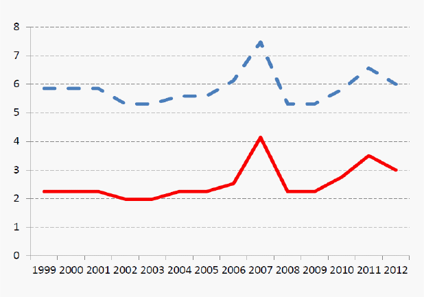
see in Figure 2 where interest rates are essentially ‡at with the deposit rate lying substantially

below the lending rate. Funds are channeled through state-owned banks to the conventional

sector mainly occupied by state-owned enterprises (SOEs). There are few investment alter-

natives for household savings, stock markets are poorly regulated and dominated by SOEs,

interest rates are set by government, the capital account is closed, and the exchange rate

is …xed or tightly managed. Through a system of strict capital controls where the state

directly manages the banking sector and …nancial intermediation, the government has been

able to maintain or suppress interest rates at below market-clearing levels. A …xed and low

interest rate was initially imposed by the government as a development strategy to subsidize

industrialization with cheap capital (see Lin, 2012). A below-market interest rate re‡ects

the government’s goal of achieving a maximum rate of capital accumulation and a high level

of employment in the SOE sector. Also, when the interest rate is …xed at a level below the

market-determined rate, SOEs would be able to earn positive pro…ts despite ine¢ ciency. The

pro…ts are, however, not redistributed back to the households, they are instead re-invested

to maximize the economy’s capital stock.

Figure 2. China’s One-Year Nominal Interest Rates (%):

Deposit (solid) and Lending (dash).

3 The Benchmark Model

We extend the SSZ model to incorporate an intrinsically valueless asset— housing, and prove

that a faster-than-income growing bubble in housing prices exists even if housing provides

no rents or utilities to investors. We emphasize the growing nature of the bubble because

the existing bubble literature often focuses exclusively on static bubbles or bubbles that

grow at the rate of technology. We focus instead on bubbles that can grow faster than the

rate of productivity growth. In particular, we show how the very expectations— that the

excessively high rate of return to capital during transition is not sustainable in the long

run— can generate a self-ful…lling housing bubble that grows faster than aggregate income

along the transition path.

3.1 The Environment

The economy is populated by overlapping generations of two-period lived agents.

Agents

work when young and consume the return from their savings when old. Agents have hetero-

geneous skills. Within each cohort, a measure N

=2 of agents have no entrepreneurial skills.

They choose to become workers and supply labor to …rms. And the rest of the agents have

entrepreneurial skills— so they choose to become entrepreneurs. Entrepreneur skills can be

transmitted from parents to children. The population N

grows at an exogenous rate :

Before the economy starts, the government owns one unit of housing (land), which is in

…xed supply. At the beginning of the …rst period, the government sells it to the market and

consumes all the proceeds.

3.2 Technology

There are two production sectors and thus two types of …rms. Labor is perfectly mobile

across the two sectors, but capital is not. The …rst sector is composed of conventional

…rms— F-…rms, which for simplicity are owned by a national bank and operated as standard

neoclassical …rms. Workers can work in either sector but deposit their savings into the

national bank. The bank lends capital to F-…rms to produce output.

The second sector is an unconventional or emerging sector, which is composed of high-

productivity …rms— E-…rms. The E-…rms are operated by entrepreneurs with over-lapping

generations. More speci…cally, E-…rms are owned by old entrepreneurs, who are residual

claimants on pro…ts and hire their own children as managers. E-…rms have higher total

factor productivity (TFP) than F-…rms. However, E-…rms cannot rent capital from the na-

tional bank.

As a result, they must self-…nance capital investment through own savings. By

We …rst use a 2-period model to illustrate our main results and then extend it to a 50-period model later

on to conduct calibrated quantitative analysis.

We will relax this assumption in a later section.

contrast, F-…rms can rend capital from the national bank at a …xed interest rate R. Accord-

ingly, along transition, an F-…rm can still survive despite with less productive technology.

Over time, however, labor is gradually reallocated from F-…rms to E-…rms as E-…rm sector’

capital stock expands.

The technologies of the two types of …rms follow constant returns to scale

F t

= (k

F t

)



F t

)

1

;

= (k

)



n

)

1

;

where y, k, and n denote output, capital stock and labor, respectively.  > 1 re‡ects the

assumption that E-…rms are more productive than F-…rms. Technological growth is constant

and exogenously given by A

t+1

= A

(1 + z) :

3.2.1 The Worker’s Problem

Workers can deposit their savings into the bank and earn a …xed interest rate R. But for

simplicity and without loss of generality, we assume that workers cannot speculate in the

housing market.

The worker’s consumption-saving problem is

max

2t+1

log c

+  log c

2t+1

subject to

+ s

= w

2t+1

= s

where w

is the market wage rate, c

; c

2t+1

and s

denote respectively the consumption when

young and old, and the worker’s savings. 

t+1

is a lump-sum transfer from the bank (to be

speci…ed below). The …rst order conditions imply

1 + 

1

Namely, the optimal level of saving is proportional to the income received when young.

In an appendix upon request, we show that allowing workers to invest in housing does not change our

results— the dynamics of housing price is una¤ected.

3.2.2 The F -Firm’s Problem

In each period, F-…rms maximize pro…ts by solving the following problem

max

F t

)



F t

)

1

 w

F t

 Rk

F t

;

where the rental rate for capital is the same as the deposit rate, R: The …rst-order conditions

are

= (1  ) k



F t

1



F t

R = k

1

F t

1

F t

(1)

This gives

= (1  ) A









1

 (1  ) A





(2)

where 



F t







1

: Note that along transition, the (detrended) wage rate,

, is

constant, due to a constant rental rate for capital. When the transition ends, all F-…rms

disappear, so equation (2) no longer holds.

3.2.3 The E-Firm’s Production

Following SSZ, we assume that young entrepreneurs get paid a management fee m

— that is

a …xed < 1 fraction of the output produced.

Therefore, the old entrepreneur’s problem

can be written as

max

(1  ) (k

)



n

)

1

 w

The …rst-order conditions imply

(1  ) (1  ) (k

)



)

1

= w

= (1  ) A









1

; (3)

where the second inequality comes from (2) based on the assumption of perfect labor mobility

across …rms. Equation (3) immediately implies a linear relationship between n

and k

= [(1  ) ]









1

A

: (4)

SSZ provides a microfoundation for young entrepreneur’s management fee as a …xed fraction of output:

There exists an agency problem between the manager and owner of the business. The manager can divert

a positive share of the …rm’s output for his own use. Such opp ortunistic behavior can only be deterred by

paying managers a compensation that is at least as large as the funds they could steal, which is a share

of output.

Such a linear relationship is obtained because of the constant interest rate R; which implies

a constant wage rate: Accordingly, labor is reallocated to E-…rms at a speed equal to the

growth of the private capital stock in the E-…rm sector. The pro…t of the E-…rm is

 (k

) = (1  ) (k

)



n

)

1

 w

= (1  )





1



 

;

where the second equality is obtained by using (4). Whenever F-…rms exist, the return

to capital in E-…rms, 

 [(1  )]





1



R, is a constant. This is because n

increases

linearly in k

: As a result, 



is a constant during the transition.

3.2.4 The Consumption-Saving Problem of the Young Entrepreneur

The young entrepreneur obtain m

= (k

)



n

)

1

as income when young, and

decides consumption and portfolio allocation in housing investment, bank deposits, and

physical capital investment. The return for capital investment is simply 

. By arbitrage,

the return to capital must be equal to or larger than the capital gains from housing:

t+1

 

: (5)

Hence, a young entrepreneur’s income when old is simply 

, where s

denotes total

savings: Therefore, a young entrepreneur’s consumption-saving problem is

max

log (m

 s

) +  log 

The …rst-order conditions imply

1 + 

1

We assume that a fraction 

of s

is invested in …rms’capital, and the rest in housing, such

that K

Et+1

= 

: Entrepreneurial housing demand is then (1  

) s

= p

The optimal portfolio 

is pinned down in equilibrium.

3.2.5 The Bank’s Problem

For exposition, we assume that each period the bank simply absorbs deposits from young

workers, rent them to F-…rms at interest rate R, and invest the rest in foreign bonds with

the same rate of return.

3.2.6 Time Line

To summarize, in each period the economic events in our model unfold as follows:

1. At the beginning of period t, production of E-…rms and F-…rms takes place. The capital

stock used by E-…rms is k

, which is from the savings of the entrepreneur when young.

The capital stock used by F-…rms is K

F t

, which is rented from the bank in the last

period (pre-determined in period t  1). Each young worker gets w

regardless which

sector they work in. Each young entrepreneur gets m

2. The young entrepreneur chooses consumption and make saving decision s

. Young

workers make consumption and deposit decisions.

3. Housing market opens. Old entrepreneurs sell housing stock held in the previous period,

Et1

; in the housing market, consume, and die. Young entrepreneurs make portfolio

decision 

and invest a fraction of wealth (1  

) s

in housing, P

4. F-…rms repay their rentals to the bank.

5. The currently old workers consume and die. So do the currently old entrepreneurs.

3.2.7 Law of Motion for K

We now derive the law of motion for the capital stock held by E-…rms. Since E-…rm is

self-…nanced, we have

Et+1

= 

1 + 

1

Note that m

= (k

)



n

)

1

= k







1

; where





n

= 

[(1  ) ]





Hence

Et+1

= 







1

1 + 

1

= 

(

[(1  ) ]









1

)

1

1 + 

1

= 



(1  ) 

1 + 

1

= 



(6)

where 





(1 )

1+

1

: The second equality follows equation (4) ; whereas the third equa-

tion follows the de…nition of 

: Equation (6) shows that the growth rate of private capital

(

Et+1

) increases with the share of entrepreneurial savings in physical capital, 

With equations (4) and (6) ; we can derive the law of motion for labor in the E-…rm sector

Et+1

(1 + z)





1 + z

3.3 Post-Transition Equilibrium

We need to characterize the equilibrium after the transition ends, i.e., when n

= 1, k

F t

= 0.

Since n

= 1, the pro…t of the E-…rm is

 (k

) =  (1  ) (k

)



)

1

Note that  (k

) now features decreasing returns to scale. The average rate of return for

capital investment is simply



t+1

Et+1

 

Et+1

) =  (1  ) (k

Et+1

)

1

t+1

)

1

: (7)

The law of motion for capital is

Et+1

= 

1 + 

1

)



N

)

1

(8)

Finally notice that

t1

Et1



1  

Et1



Et1

t1



1  

Et1





t1

(1  ) 

1 + 

1

Et1

(9)

Note that 

(

) is a function of 

3.3.1 Housing Demand and Housing Price

We now determine the housing demand by young entrepreneurs and the equilibrium housing

price. Note …rst that the housing demand satis…es

= P

Consider two cases:

Case 1: R <

t+1

= 

To derive the key equation on 

; note that

= (1  

) s

= (1  

)

1 + 

1

)



N

)

1

(10)

Case 2:

t1

< 

: In this case, entrepreneurs will not invest in housing, i.e. 

= 0.

Then P

= 0. In this paper, we focus on the equilibrium with housing.

3.4 Characterizing the Equilibrium

Since all per-capita variable (except for n

) grow at the rate A

; we detrend all per capita

variables as bx

= x

3.4.1 Steady State

At the steady state, we have



E

=  (1  )





=



1

=  (1  )



1 + 

1



(1 + z) (1 + )





;

where the second equality is derived from (25). With the no-arbitrage condition b etween

housing and physical capital, we have

 (1  )



1 + 

1



(1 + z) (1 + )





t+1

= (1 + z) (1 + )

This gives the share of saving of E-…rm in physical capital at the steady state





=  (1  )



1 + 

1



= (11)

Intuitively, the larger is the returns to capital for the entrepreneur, as captured by  (1  ) ;

the larger is the share of entrepreneurial savings in physical capital. On the other hand, the

larger is and , which re‡ects a higher income of young entrepreneur and their saving

propensity, the lower is the returns to physical capital and thus the lower would b e the share

of entrepreneurial savings in physical capital.

Note that in our economy, we need 



< 1 for housing to exist: This implies that without

housing the private return to physical capital by entrepreneurs will b e below the balanced

growth rate. This implies the following parameter restriction

 (1  )



1 + 

1



< (12)

Intuitively, a larger a¤ects the rate of returns for capital for the old entrepreneur in two

way: …rst, it directly reduces the output share accrued to the old entrepreneur; second, by

increasing the output share of the young entrepreneur, it increases the capital accumulated

by the young and thus pushing down the marginal product of capital. In addition, we need

to assume the returns for housing is larger than the bank deposit rate

t+1

= 

E

= (1 + z) (1 + ) > R:

To summarize, we have the following equations at steady state,









1



1 + 

1



(1 + z) (1 + )

1

(13)



E

=  (1  )





=



1

(14)

H

h = p

H



(15)

H



= (1  



)

1 + 

1







1

: (16)

3.4.2 Existence and Normative Implications of Bubbles

Di¤erent from the neoclassical growth model, in our economy, the old entrepreneur’s returns

to capital, 

; is only a fraction, 1  ; of the marginal product of capital for E-…rms, which

is the social rate of returns to capital. This implies that housing bubbles may exist even

under dynamic e¢ ciency. The condition for dynamic e¢ ciency is that

=@k





> (1 + z)(1 + v) (17)

At steady state, with (13) under 



= 1; (17) implies

< (1 + 

1

): (18)

Intuitively, the smaller is, the smaller is the steady-state capital and the higher is its

marginal product. Also, similar to standard OLG models, a higher  or a lower  make the

economy less likely to be dynamic ine¢ cient.

An interesting issue is the normative implication of bubbles in an economy without

dynamic ine¢ ciency. This implication is interesting because bubbles can exist in our model

without dynamic ine¢ ciency, and they reduce the aggregate resource available for aggregate

consumption. In Proposition 1, we show that the following condition is su¢ cient for bubbles

to exist and to crowed out aggregate consumption of the investors:

+  (1  )

< (1 + 

1

) (19)

Note that <

+(1 )

: Hence, condition (19) satis…es equation (18), which implies that

the economy is dynamically e¢ cient.

A combination of (12) and (19) gives the following parameter restriction

 (1  )



1 + 

1



< < (1 + 

1

) [ +  (1  )] (20)

We now derive the normative implication of bubbles under condition (20). De…ning the

aggregate consumption at period t of agent j 2 fw; Eg as bc

= bc

+ bc

(1 + v)

1

, we have

the following

Proposition 1 : Given (20), a housing bubble reduces aggregate consumption and welfare—

measured by the lifetime utility of both the workers and the entrepreneurs at the steady state.

Proof: see Appendix.

The intuition is clear. When the economy is dynamically e¢ cient, a housing bubble will

reduce the aggregate resource available for consumption. If the marginal product of capital

is su¢ ciently high, then choosing housing as an alternative store of value would crowed out

capital and reduce consumption.

Regarding social welfare, since the workers’ wage income decreases with capital stock

but the rate of return to saving (the deposit rate) is …xed, their lifetime utility decreases as

a results of housing bubble. For the entrepreneurs, the utility loss due to a fall in lifetime

entrepreneurial income dominates the welfare gain arising from the income e¤ect of a higher

capital return. Hence, both workers and entrepreneurs su¤er welfare losses.

Proposition 2 Given (20), a housing bubble reduces the aggregate consumption of workers

(after the transition ends) and the aggregate consumption of entrepreneurs.

Proof: see Appendix.

Since the wage rate is a constant, it is una¤ected by the presence of a bubble along

the transition. Hence, the welfare of workers along transition is una¤ected by the bubble.

However, when the transition ends, the wage rate changes with the physical capital. So a

bubble reduces the welfare of all workers in the post-transition period.

For entrepreneurs along transition, the rate of return to capital is una¤ected by the

presence of a bubble. Hence, given the initial capital stock, the utility of the old and young

entrepreneurs alive in the …rst p eriod are unchanged when a housing bubble is introduced.

From the second perio d on, however, the income of the young entrepreneur will fall due to

the crowding out of capital by the bubble. Hence, all entrepreneurs along transition will

have lower welfare (since the return to capital is constant). For entrepreneurs alive in the

post-transition period, the rate of return to capital is not constant but higher than that at

the steady state. So the loss in income due to a reduction in capital stock is still higher than

the gain from the higher rate of return to capital. Hence, they also su¤er welfare losses as a

result of housing bubble.

3.4.3 The Housing Price to Output Ratio

We now characterize the dynamics of housing price-to-income ratio, one of the key focuses

of the paper. We …rst establish a lemma about the dynamics of the share of entrepreneurial

savings in housing.

Lemma 3 Throughout the transition and post-transition period, the share of entrepreneurial

savings in physical capital is constant,







1 + 

1



(1  )

; 8t: (21)

Proof: see Appendix.

To understand the intuition b ehind Lemma 3, we plug the value of 

into the law of

motion for capital

Et+1

= (1  )  (K

)



n

)

1

(22)

= 

(22) implies that not only capital accumulated by entrepreneur is linear in current output, but

is a constant fraction of output over time. The higher is the fraction of output attributable

to the old entrepreneurs, as captured by (1  ) ; the larger is the share of current output

going to the end-of-period capital stock. And this constant fraction of output devoted to

capital accumulation is achieved by the portfolio choice of entrepreneurs according to (21) ;

which is constant under constant marginal propensity to save in our two-period model. With

Lemma 3, the following proposition captures the dynamics of housing price to output ratio.

Proposition 4 The housing price-to-output ratio and housing price-to-wage ratio in the

post-transition period are constant, while they are both increasing during the transition.

Proof: We …rst prove that the ratio of housing price to aggregate output is constant

in post-transition period. Since the growth rate of housing price is equal to 

t+1

; this is

equivalent to prove that the growth rate of aggregate output in post-transition period is

equal to 

t+1



t+1

(1  ) 

(1  )  = 

t+1

;

where the second equality is obtained by the de…nition of 

t+1

and (22) : Therefore, the

housing price to output ratio is constant in post-transition period. Since wage is a constant

fraction (1  ) (1  ) of aggregate output, it is straight forward that the housing price-

wage ratio is constant in post-transition period.

Along the transition stage, we have

t+1

F t+1

Et+1

F t

: Equation (1) implies that the

growth rate of output by F-…rms follows

F t+1

F t

F t+1

=

F t

=

F t+1

F t

< 0

Therefore, we have

t+1

Et+1

= 

t+1

;

where the proof of the second equality follows the same procedure as that for the post-

transition perio d. As a result, the housing price to output ratio will increase along the

transition.

The intuition of Proposition 4 is as follows. In the post-transition period, the economy

essentially becomes a neoclassical economy. In our simple model with full capital deprecia-

tion, the end-of-period physical capital is proportional to the current aggregate output, with

the share equal to the next-period share of output going to old entrepreneur. Hence, the

housing price to output ratio is constant during the post-transition period. Note that this

property also holds in a neoclassical framework (with complete capital depreciation).

During the transition, however, the aggregate output growth is an average of the output

growth of the E-…rms and F-…rms. Since F-…rms keep downsizing due to labor reallocation,

the aggregate output growth is less than the output growth rate of the E-…rms, which equals

to the returns to capital for the old entrepreneur. Therefore, the housing price will grow

faster than the aggregate output (and wage rate, which is constant) along transition.

3.5 Numerical Algorithm

During transition, we have the following equation to determine labor allocated to E-…rms:

= [(1  ) ]









1

A

= [(1  ) ]









1

=

We check if n

> 1: If so, we set n

= 1:

Also, we have the following equations for both transitional and post-transitional periods

= (1  ) (1  )









1

(23)



=  (1  )



[(1  ) = bw

]

1





1



(24)

Et+1

= 



)

1



(1 + ) (1 + z)



1 + 

1



(25)



t+1

(1 + z) (1 + ) =

t+1

if 

< 1

0 if 

= 1

(26)

= bp

h (27)

= (1  

)



)

1



1 + 

1



We assume the second transition period takes T p eriods. At period T , the economy

enters the steady state. The algorithm to solve for the transition takes the following steps:

1. guess the sequence of f

T 1

t=1

2. given k

, compute

; bw

; 

;

Et+1

; bp

; h

according to the above equations.

3. Check the following condition for each period t = 1; 2; ::; T  1



= 1 



1 + 

1





)

1

(28)

and (since 

T +1

not known)

T +1









1



1 + 

1



(1 + z) (1 + )

1

4 Numerical Results

We use the following parameter values for the numerical exercise:  = 0:3;  = 0:96

;

= 0:62 (note > = :5691).  = 4:98: R = 1:0147; z = 0:0147;  = 0: h = 1; z = 0:0147:

These parameters satisfy the condition (20) to ensure housing bubbles exist in an economy

with dynamic e¢ ciency. We also choose k

= 0:031; such that the economy experiences a

transition stage. Note that a smaller k

tends to prolong the transition. But it also makes

wage and thus the saving rate of the young worker smaller. At the same time, a smaller k

makes 1  n

and thus k

F 1

larger. This will also tend to make smaller the bank deposit net

of capital demand by F-…rms, as well as the housing demand by the banking sector.

4.1 Benchmark Results

Figure 3 shows the dynamics of the benchmark economy. In Panel A, capital in E-…rms

increases at a faster rate during the …rst three periods than thereafter. This is because

the marginal product of capital is constant when F-…rms exist, as labor is kept reallocating

from F-…rms to E-…rms. This can be seen in Pane B. At period 4, the transition is over, as

= 1. Panel C shows that aggregate output follows a similar growing pattern to that of

physical capital in E-…rms.

Panel D shows the consumption pattern during transition. Notice that during transition,

consumption of E-…rms grows fast while that of workers is essentially ‡at due to a constant

wage pro…le. As a result, most of the increase in aggregate consumption is due to the increase

of consumption of entrepreneurs. In Panel E, we see that during transition, the aggregate

rate of returns for capital, which is weighted average rate of returns for capital for E-…rms

and F-…rms is increasing, since the capital share of E-…rms keep increasing. However, during

the post-transition stage, the aggregate returns to capital, which is simply the E-…rm’s rate

of returns to capital, starts to decline. In Panel F, total factor productivity increases along

transition, since resources are reallocated to the E-…rm, which is more productive. However,

in the post-transition stage, the (detrended) TFP, which is the productivity of E-…rms, is

constant.

1 2 3 4 5 6

0.2

0.4

Panel A: Capital in E Firm

1 2 3 4 5 6

0.5

Panel B: Labor in E Firm

1 2 3 4 5 6

0.5

1.5

Panel C: Aggregate Output

1 2 3 4 5 6

period

Panel D: Consumption

1 2 3 4 5 6

Panel F: Total Factor Productivity

period

1 2 3 4 5 6

1.5

Panel E: Returns to Capital

period

Total

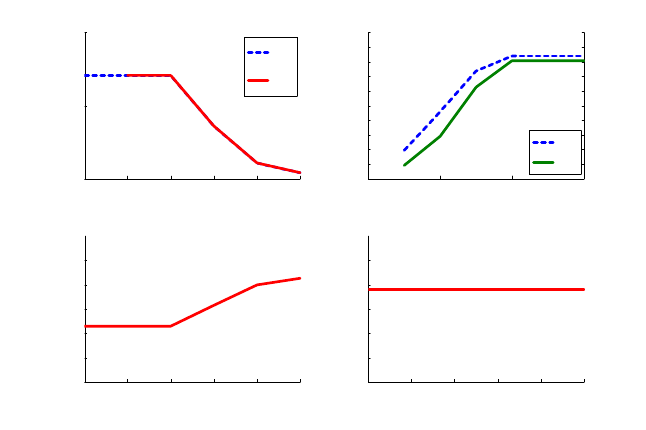
Figure 3. Macro Variables in the Benchmark Economy.

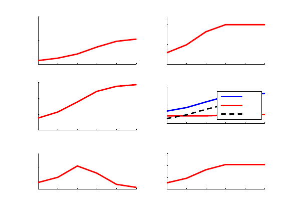
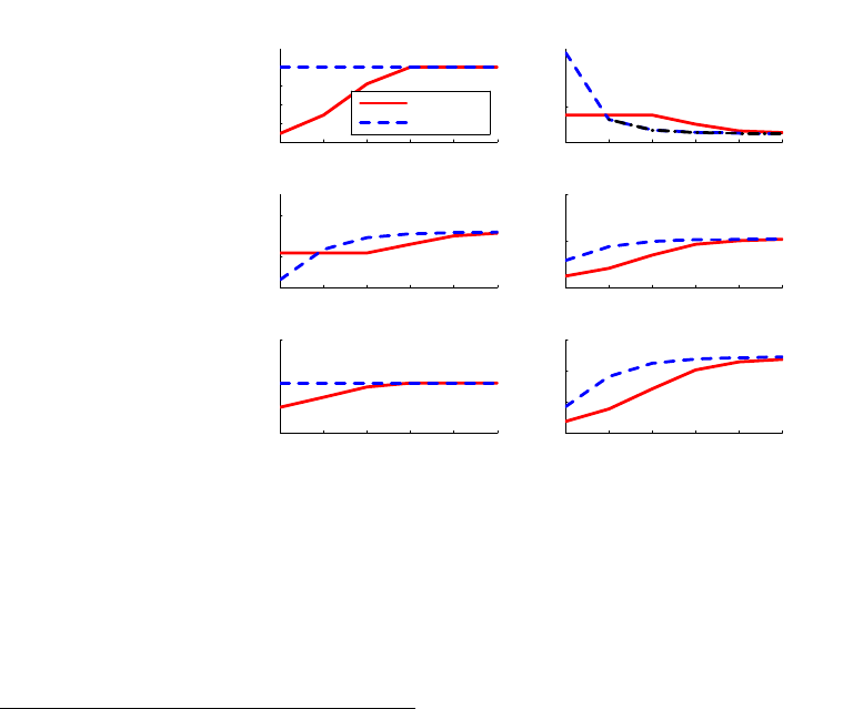
Figure 4 shows the dynamics of housing prices and share of entrepreneurial savings in

housing. Panel A shows the detrended housing prices growth rate, which track the returns

for capital in E-…rms. Note that the rate of returns for physical capital starts to fall in

period 4, when the transition is over. As a result, the growth rate of housing price is high

along transition, but exhibits a declining pattern in the post-transition period. Eventually,

housing prices in the long run equal the balanced growth rate of the economy. Panel B shows

the ratio of housing price to income. We see that the housing price to wage ratio increases

dramatically. This is because, as Panel C shows, that wage rate is constant along transition

due to the presence of F-…rms and labor reallocation. Similarly, the ratio of housing price

to aggregate output, P

; keeps increasing during transition, but becomes a constant in

the post-transition stage. Again, this is because during transition, housing prices grows at

a rate faster than the growth rate of the aggregate output, as Proposition 3 argues.

Finally, in Panel D, we see that the share of E-…rms’saving in housing is constant in this

two-period economy. Note that even entrepreneurs along transition demand housing despite

a high rate of returns for capital. This is essentially because those entrepreneurs alive during

transition expect that the high capital returns driven by cheap labor and resource relocations

are not sustainable in the long run, which induces future investors to seek alternative store

of value for their growing wealth. This pushes up the expected rate of returns for housing

even during transition. As a result, entrepreneurs born along transition in our benchmark

economy have incentive to hold housing.

1 2 3 4 5 6

1 .5

P a ne l A : R e tu rn to K vs. H

rho

0 2 4 6

0.01

0.012

0.014

0.016

0.018

0.02

0.022

0.024

0.026

0.028

0.03

Price to Output Ratio

Panel B: Housing Price/Income

0 2 4 6

0.02

0.03

0.04

0.05

0.06

0.07

0.08

0.09

0 .1

0.11

0.12

Price to Wage Ratio

P /Y

P /W

1 2 3 4 5 6

0.3

0.35

0.4

0.45

0.5

0.55

Panel C: W age Rate

1 2 3 4 5 6

0.05

0.1

0.15

0.2

0.25

Panel D: Share of E Firm Savings in Housing

Figure 4. Housing Dynamics in the Benchmark Economy

4.2 Counterfactual Experiments

We now explore the key ingredients in our model that help to sustain a high growth rate of

housing price along the transition. To this end, we conduct several counterfactual experi-

ments, in which we shut down one of the ingredients at a time. We examine two ingredients:

(i) the role of the entrepreneurial returns to capital at the steady state, (ii) the role of …rm

heterogeneity.

4.2.1 The Role of Bubbles for Transition and Welfare

We would like to explore the role of bubbles for the transition as welfare. Similar to all studies

on bubbles, in our model, the existence of bubbles rely on the assumption that at steady

state, the rate of returns for capital for entrepreneurs is lower than the balanced-growth rate

(though the economy can be dynamic e¢ cient). Therefore, to eliminate housing demand by

entrepreneurs at the steady state, we impose an output subsidy to E-…rms only at the steady

state to equalize the rate of returns to capital for entrepreneurs at the steady state to the

balanced growth rate. We keep all other parameters the same as before.

Accordingly, an

E-…rm’s problem at steady state becomes

max

(1 + 

)



(1  ) (k

)



n

)

1

 w



Note that the subsidy is proportional to the net pro…t. Accordingly, the …rst-order condition

for n

and the capital-labor ratio is still the same as in our benchmark economy. The pro…t

of the entrepreneur is

 (k

) = (1 + 

) 

Figure 5 plots the transitional dynamics for both the counterfactual and the benchmark

economies. Panel A shows that throughout the transition, housing price is zero. Panel B,

C and D suggest an improvement of allocative e¢ ciency in this counterfactual experiment,

as both capital accumulation by E and aggregate output are higher than their counterparts

in the benchmark economy. Moreover, the transition period is shorter, as labor demand by

E-…rms has reached 1 in period 3. Panel E and F show that the counterfactual economy

generates higher aggregate consumption, and consumption for both entrepreneurs and work-

ers. Intuitively, more entrepreneurial savings towards capital investment also increase future

entrepreneurs’permanent incomes.

We …nd that the transitional pattern of this economy, except for the returns to capital, is equivalent to

another economy in which entrepreneurs are shut down from access to housing markets.

1 2 3 4 5 6

0.05

0.1

Panel A: Housing Price

Bench.

Counter.

1 2 3 4 5 6

0.1

0.2

0.3

0.4

Panel B: Capital in E Firm

1 2 3 4 5 6

1.5

2.5

Panel D: Aggregate Output

1 2 3 4 5 6

0.5

P a ne l C : L ab or in E Firm

1 2 3 4 5 6

0.5

1.5

Panel E: A ggregate Consumption

1 2 3 4 5 6

0.5

1.5

Panel F: Consumption of Different A gents

HH, benc.

HH, counter.

E, bench.

E, counter.

Figure 5: Transition in Economy without Dynamic Ine¢ ciency

In summary, our experiment shows that housing bubbles crowds out physical capital,

prolongs transition and reduces consumption for both entrepreneurs and workers.

4.2.2 The Role of Firm Heterogeneity

We now examine the second key ingredient of our model: heterogeneous …rms in both pro-

ductivity and access to …nancial markets. This feature allows the existence of a transition

stage where labor is reallocated from F-…rms to E-…rms. Accordingly, the marginal product

of capital for E-…rms is constant along the transition. We argue that this feature is key to

sustaining the persistently high growth rate of housing prices during transition.

To examine the role of heterogeneous …rms, we construct an counterfactual economy

where F-…rms are absent. In other words, all labor is employed in E-…rms at the very

beginning. As a result, all E-…rms are neoclassical in nature except that they are self-

…nanced. We still keep the ingredient of dynamic ine¢ ciency in the long run. Therefore,

both the counterfactual and the benchmark economy share the same steady state.

In Panel A of Figure 6, we see that labor demand for E-…rms is always 1. Accordingly, as

entrepreneurs accumulate capital, the return for capital drops quickly from an initially high

level to a very low level at the steady state (Panel B). In Panel C, wage rate starts to increase

at the beginning of the economy. Panel D shows that housing price starts at a higher level,

but overtime the growth of housing prices slows down, in contrast to a fast increase during the

transition stage of the benchmark economy. Accordingly, housing price-to-aggregate output

ratio is constant (Panel E). Finally, throughout transition, aggregate consumption is now

higher than the benchmark economy, though they converge to the same steady state. This

implies that the negative e¤ect of housing on aggregate consumption is particularly large in

our benchmark economy. The reason is that in our benchmark economy during transition,

the rate of returns to capital is very high due to labor reallocation. Therefore, the welfare

loss of the crowding-out e¤ect of housing is much larger in our benchmark economy.

In summary, the presence of …rm heterogeneity (in both technology and access to …nancial

markets) helps maintain a high rate of return to capital during the transition. Accordingly,

with entrepreneurial demand for housing, the equilibrium growth rate of housing prices is

high along the transition. Without the presence of F-…rms, the dynamics of housing prices

essentially follows the growth rate of the aggregate output. As a result, the housing price-

to-output ratio is constant without …rm heterogeneity. Moreover the welfare loss of the

economy due to housing as bubbles is much larger with …rm heterogeneity.

1 2 3 4 5 6

Panel B: Return to Physical Capital and H

1 2 3 4 5 6

0.05

0.1

Panel D: Housing Price

1 2 3 4 5 6

0.4

0.6

Panel C: Wage Rate

1 2 3 4 5 6

0.05

Panel E: Housing Price/Aggregate Output

1 2 3 4 5 6

0.2

0.4

0.6

0.8

Panel A: Labor in E firm

Bench.

w/o F Firm

1 2 3 4 5 6

0.5

1.5

Panel F: Aggregate Consumption

Figure 6: Transition in Economy without Firm Heterogeneity

5 Quantitative Analysis

[to be added]

Note that in this counterfactual economy, housing still causes welfare loss to workers and entrepreneurs,

since the economy is dynamic e¢ cient and satis…es (19) :

6 Conclusion

This paper provides an explanation to the great housing bo om in China. In particular, we

show in an endogenous growth model that the great housing bo om can be a rational bubble

arising naturally from China’s unprecedented economic transition, which features persistent

and exceptional high returns to capital— driven largely by massive reallocations of cheap

labor from unproductive sectors to productive sectors. Since the transition will eventually

come to an end, capital returns are expected to decline sharply in the future. Based on

such rational expectations, investors opt to seek alternative stores of value for their growing

wealth. Given China’s underdeveloped …nancial market and capital controls, investors opt

to speculate in the housing market in an early stage by holding the housing stock as a

hedge for their wealth in addition to capital. This generates a strong speculative demand

for housing investment, which recti…es the anticipated housing price boom and leads to a

growing housing bubble with a rate of return equal to that of capital. Consequently, the

economy exhibits an increasing housing price-to-income ratio and an increasing share of

housing investment in GDP during the transition. Such a growing housing bubble crowds

out capital accumulation, prolongs economic transition and reduces welfare for all agents in

the economy.

There are many issues left for future research concerning the e¤ects of housing bubble

in China. For example, housing bubble reduces the private sector’s incentive to innovate.

Because of the relatively low risk, low entry costs, low technology, and high pro…ts in housing

investment, the housing bubble has enticed many productive and high-tech …rms in China

to reallocate resources from R&D to the real estate market. In an economy transiting from

labor intensive economy to capital intensive economy, such resource misallocation can be

very costly: It may substantially prolong China’s economic transition and reduce China’s

TFP growth, especially when its population is aging fast and labor costs rapidly rising. We

plan to quantify such resource misallocation within our framework in future works.

Furthermore, the rapidly rising housing prices have caused great social concerns as more

and more low-income households are excluded from the housing market— because their in-

come growth falls behind housing price growth. The housing price growth is driven largely

by upper middle income class who has enjoyed the most rapid income growth during the

economic development. The inequality in wealth distribution in China has thus widened and

exacerbated recently, mainly because of the rising housing prices. Again, this is an important

issue for our future research.

References

[1] Buera, F. and Y. Shin (2011), “Productivity Growth and Capital Flows: The Dynamics

of Reforms”, working paper.

[2] Caballero, R., and A. Krishnamurthy (2006), “Bubbles and Capital Flow Volatility:

Causes and Risk Management,”Journal of Monetary Economics, 53(1): 35— 53.

[3] Yongheng Deng, Randall Morck, Jing Wu and Bernard Yeung, “Monetary and Fiscal

Stimuli, Ownership Structure, and China’s Housing Market,” NBER working paper

16871.

[4] Farhi, E. and J. Tirole (2012), “Bubbly Liquidity,”Review of Economic Studies, 79(2),

678-709

[5] Kocherlakota, N. (2009), “Bursting Bubbles: Consequences and Cures,” mimeo, Uni-

versity of Minnesota.

[6] Martin, A. and J. Ventura (2012), “Economic Growth with Bubble,” American Eco-

nomic Review, 102(6), 3033-3058.

[7] Moll (2012), “Productivity Losses from Financial Frictions: Can Self-…nancing Undo

Capital Misallocation?,”working paper.

[8] Song, Zheng, Kjetil Storesletten and Fabrizio Zillibotti (2011), “Growing Like China,”

American Economic Review, 101, 196-233.

[9] Tirole, J. (1985), “Asset Bubbles and Overlapping Generations,”Econometrica, 53 (6),

1499-1528.

[10] Ventura, J. (2011), “Bubbles and Capital Flows,”Journal of Economic Theory, 147(2),

738-758.

[11] Wu, Jing, Joseph Gyourko, Yongheng Deng (2012), “Evaluating Conditions in Major

Chinese Housing Markets," Regional Science and Urban Economics, 42 (3): 531-543.

[12] Yang, Dennis Tao, Vivian Weijia Chen, Ryan Monarch (2010), “Rising Wages: Has

China Lost its Global Labor Advantage?”Paci…c Economic Review, 15(4), 482-504.

[13] Wei, Shangjin, Xiaobo Zhang and Yin Liu (2012),“Status Competition and Housing

Prices: Some Evidence from China”, working paper.

7 Appendix

7.1 Proof of Propositions

In this section, we prove the various propositions.

Proof of Proposition 1. To prove this proposition, consider a counterfactual economy

without housing, i.e. 

= 1. According to (13) ; introducing housing (i.e. 

< 1)

at the steady state would reduce physical capital. Hence, we only need to show under

which condition reducing physical capital at steady state reduces aggregate consumption for

both entrepreneurs and workers. Aggregating the budget constraint of the young and old

entrepreneurs at period t, we get

= bm

+ 



Et+1

(1 + z)(1 + v) (29)

In our steady state analysis below, we drop the time subscript for notation concision.

Taking the derivative of the right side of (29) with respect to

at the steady state, we

can obtain the following su¢ cient condition for introducing bubbles to reduce aggregate

consumption for entrepreneurs.

@m=@k

+ 





> (1 + z)(1 + v) (30)

On the left side of (30) ; @m=@k

is the marginal cost on the young entrepreneur’s income

of a reduction in physical capital. The second argument, 

; refers to the marginal pro…t

loss to the old entrepreneur of a reduction in physical capital. Finally, 





is the

marginal bene…t of reducing capital in terms of an increase in marginal product. The right

side of (30) is the returns for bubbles at the steady state. Using the de…nition of m and 

;

it is easy to show that (30) can be rewritten as



1 

+ 





> (1 + z)(1 + v) (31)

At steady state, with 

= 1; we obtain the value of 

by combining (14) and (13)



= 



1 + 

1



(1 + z) (1 + n)

1 

(32)

Plugging (32) into (31), we get

(1 + 

1

) >

+ (1  )

(33)

Condition (33) is the same as (19) :

To obtain the impact of bubbles on aggregate consumption of workers at steady state,

we simply aggregate the worker’s budget constraint at period t

+ bs

= bw

+ Rbs

t1

= [(1 + z)(1 + n)]

Using bs

= bw=(1 + 

1

), at the steady state, we have



1 +



(1 + z) (1 + n)

 1



=(1 + 

1

)



bw (34)

It is easy to show that the coe¢ cient for bw on the right side of (34) is positive. And since

bw = (1  ) (1  )









1

; we have @ bw=@

> 0. Hence, introducing housing reduces

aggregate consumption for the worker at the steady state.

Now we prove the welfare implication of housing for both the worker and entrepreneur.

For the worker, simply notice that their deposit rate is …xed at R: Hence a reduction of

permanent income, bw; will reduce their lifetime utility. For the entrepreneur, the lifetime

utility can be expressed as

log (m

 s

) +  log 

= log





(1 + )  (1  )



+  log 

=

= (1 + ) log 

  log 

+ C (35)

where C is a constant as a function of parameters. Plugging the steady-state value of 

and k

into (35) ; we get

(1 + ) log 

  log 

+ C

= (1 + ) log 

1 



1 + 

1





(1 + z) (1 + n)





1



1 + 

1



(1 + z) (1 + )

1

 log 

+ C



 (1 + )

1  

 



log 

where

C is another constant as a function of parameters. Hence, introducing housing, i.e.

reducing 

; reduces the welfare if

(1+)

1

> ; that is, 



1 + 

1



> 1  : Note that the

joint of participation and incentive constraint of the young entrepreneur implies m = y

w = (1  ) (1  ) y

; which gives the following parameter restriction > (1  ) (1  ),

or equivalently

+(1 )

> 1  : Therefore, with the assumption (19) ; introducing housing

will reduce the lifetime utility of the entrepreneur at the steady state.

Proof of Proposition 2: The proof of welfare implication for the workers and entrepre-

neurs along transition is straightforward. For the entrepreneur in the post-transition period,

we need to prove

=@k

+ 





< 0: (36)

In the post-transition period, since

increases monotonically. (36) simply says that the

net marginal bene…t (loss) of an increase (decrease) in capital is higher when

is smaller.

Using (31) and the de…nition of 

; the left side of (36) is

=@k

+ 





=  (1  )

(1  )





2



1

< 0:

Proof of Lemma 1. We now prove that the share of entrepreneurial savings in housing

is constant over time. Using the housing market clearing condition, we have

(1  

)

1 + 

1

)



n

)

1

= P

H (37)

Forwarding (37) by one period, and with (K

Et+1

)



t+1

n

Et+1

t+1

)

1

= K

Et+1



t+1

= [ (1  )],

equation (37) can be rewritten as



1  

Et+1



1 + 

1



t+1

Et+1

 (1  )

= P

t+1

H (38)

With the law of motion for capital (8) ; (38) can be rewritten as



1  

Et+1



1 + 

1



t+1

 (1  )



1 + 

1

)



n

)

1

= P

t+1

H (39)

Dividing (39) by (37)for all t; we have

1  

Et+1

1  



1 + 

1



t+1

 (1  )

t+1

= 

t+1

; (40)

or simply

1  

Et+1

1  



1 + 

1

 (1  )

= 1 (41)

Equation (41) is a …rst-di¤erence equation capturing the dynamics of 

: One solution

to (40) is that



 (1  ) (1 + 

1

)

; 8:

7.2 Allowing Entrepreneurs to Borrow against Housing

A potential remedy for credit misallocation is to allow access of E-…rms to bank credit. Note

that since the lending rate is …xed and below the rate of return to housing, banks would not

be willing to lend to E-…rms at the low interest rate. Moreover, in China, entrepreneurs face

limited enforcement in debt repayment. Hence, banks can lend to E-…rms with housing (or

land) as collateral.

We assume that each young entrepreneur can borrow against his housing purchase at the

end of each period

 #P

; 0  #  1 (42)

where the left-hand side of (42) is the bank loan (plus interest payment) to young entrepre-

neurs, which has to be less than or equal to a fraction # < 1 of the value of housing purchase.

In our benchmark economy, # = 0: We now consider a permanent increase in #: It is easy to

show that the law of motion for capital and housing now follow

Et+1



 # (1  

)



(43)

(1  

) R

 # (1  

)



(44)

where 





(1 )

1+

1

. Clearly, a change in # (expected or unexpected) a¤ects the

entrepreneurial capital and housing demand via two channels: (i) a direct e¤ect: an increase

in # increases the amount of borrowing by entrepreneurs and thus increases demand for

both capital and housing; (ii) an indirect e¤ect via 

: since both the returns for physical

capital and housing is larger than the borrowing cost, R

; entrepreneurs will borrow to the

credit limit, which implies an increase in the share of housing in the asset portfolio held

by entrepreneurs, i.e. 

fall in responses to anticipated or unanticipated increases in #.

Accordingly to (44) ; this would reinforce the positive impact on housing demand.