
Centre for
Multilevel
Modelling
The development of this E-Book has been
supported by the British Academy.
Multiple Regression practical
In this practical we will look at regressing two different predictor variables individually on a response, followed by a model containing both
of them. We will also look at a second approach to doing this. This work builds on the earlier simple linear regression practical.
Family background is known to be an important predictor of educational achievement, but as a construct it encompasses many different
dimensions of parental resources, some of which may be more important for children’s learning. In this practical, we explore how two
aspects of parental resources – an indicator of a family’s wealth and the degree of emotional support provided by parents for a child’s
learning – are associated with performance on the PISA science test (SCISCORE). The first predictor variable is WEALTH, which is derived
from reports of whether the family owns eight items, such as a car, a computer and a room of the child’s own. The second predictor
variable is EMOSUPS, which is derived from four items with which students rated their strength of agreement, e.g. “My parents support my
educational efforts and achievements” (see PISA datafile description for further details).
Multiple Regression in SPSS worksheet (Practical)
We start by running the first linear regression to look at if there is a significant (linear) effect of WEALTH on SCISCORE. This is done in
SPSS as follows:
Select Linear from the Regression submenu available from the Analyze menu.
Copy the Science test score[SCISCORE] variable into the Dependent box.
Copy the Family wealth score[WEALTH] variable into the Independent(s) box.
Click on the Statistics button.
On the screen appears add the tick for Confidence Interval to those for Estimates and Model fit.
Click on the Continue button to return to the main window.
Click on the OK button to run the command.
SPSS will produce several tabular outputs but here we will focus on only the model summary and coefficients tables that can be seen
below:
Model Summary
Model
R R Square Adjusted R Square Std. Error of the Estimate
1 .090 .008 .008 102.19569
a. Predictors: (Constant), Family wealth score
Here we see some fit statistics for the overall model. The statistic R here takes the value .090 and is equivalent to the Pearson correlation
coefficient for a simple linear regression, that is a regression with only one predictor variable. R squared (.008) is simply the value of R
squared (R multiplied by itself) and represents the proportion of variance in the response variable, SCISCORE explained by WEALTH. The
table also includes an adjusted R square measure which here takes value .008 and is a version of R squared that is adjusted to take account
of the number of predictors (one in the case of this simple linear regression) that are in the model. We next look at the coefficients table
which is shown below:
Coefficients
Model
Unstandardized Coefficients Standardized Coefficients
t Sig.
95.0% Confidence Interval for B
B Std. Error Beta Lower Bound Upper Bound
1 (Constant) 519.868 1.621 320.763 .000 516.690 523.045
Family wealth score 9.290 1.450 .090 6.406 .000 6.447 12.133
This table often gives the most interesting information about the regression model. We begin with the coefficients that form the regression
equation. The regression intercept (labelled Constant in SPSS) takes the value 519.868 and is the predicted value of SCISCORE when
WEALTH takes value 0. The regression slope, or unstandardised coefficient, (B in SPSS) takes value 9.290 and is the amount by which we
predict that SCISCORE changes for an increase of 1 unit in WEALTH.
Both coefficients have associated standard errors that can be used to assess their significance. SPSS also reports a standardised coefficient
(the Beta) that can be interpreted as a "unit-free" measure of effect size, one that can be used to compare the magnitude of effects of
predictors measured in different units. Here Beta takes the value .090 which represents the predicted change in the number of standard
deviations of SCISCORE for an increase of 1 standard deviation in WEALTH.
To test for the significance of the coefficients we need to form test statistics which are reported under the t column and these are simply B
/ Std.Error. For the slope on WEALTH the t statistic is 6.406 and this value can be compared with a t distribution to test the null hypothesis
that the slope is 0. We can see the resulting p value for the test under the Sig. column. The p value (quoted under Sig.) is .000 (reported as
p < .001) which is less than 0.05. We therefore have significant evidence to reject the null hypothesis that the slope coefficient on WEALTH
is zero.
a

We can also check if the intercept is different from zero though this is often of less interest. For the intercept here the t statistic is 320.763
and the p value (quoted under Sig.) is .000 (reported as p < .001) which is less than 0.05. We therefore have significant evidence to reject
the null hypothesis that the intercept is zero.
The final two columns give confidence intervals for the coefficients and so a 95 percent confident interval for the intercept takes values
between 516.690 and 523.045.
Similarly a 95 percent confidence interval for the slope for WEALTH takes value between 6.447 and 12.133. Here we see the confidence
interval does not contain 0 which corresponds to the fact we could reject the null hypothesis that the slope was 0.
We will next run the second linear regression to look at if there is a significant (linear) effect of EMOSUPS on SCISCORE. This is done in
SPSS as follows:
Select Linear from the Regression submenu available from the Analyze menu.
Remove the Family wealth score[WEALTH] variable from the Independent(s) box.
Copy the Parental emotional support score[EMOSUPS] variable into the Independent(s) box.
The other options will be remembered from last time.
Click on the OK button to run the command.
The model and coefficients tables for this second model can be seen below:
Model Summary
Model
R R Square Adjusted R Square Std. Error of the Estimate
1 .119 .014 .014 101.43961
a. Predictors: (Constant), Parental emotional support score
This time we see some fit statistics for the regression with EMOSUPS. The statistic R here takes the value .119. R squared (.014) represents
the proportion of variance in the response variable, SCISCORE explained by EMOSUPS. This time the adjusted R square measure takes
value .014. We next look at the coefficients table which is shown below:
Coefficients
Model
Unstandardized Coefficients Standardized Coefficients
t Sig.
95.0% Confidence Interval for B
B Std. Error Beta Lower Bound Upper Bound
1 (Constant) 524.067 1.435 365.298 .000 521.254 526.879
Parental emotional support score 12.387 1.456 .119 8.507 .000 9.532 15.242
This time the coefficients that form the regression equation are as follows: The regression intercept takes value 524.067 while the
regression slope takes value 12.387 and is the amount by which we predict that SCISCORE changes for an increase of 1 in EMOSUPS.
This time under the Beta column the standardised slope takes value .119 which represents the predicted change in SCISCORE in standard
deviation units for an increase of 1 standard deviation in EMOSUPS.
For the slope cofficient on EMOSUPS the t statistic is 8.507 and this value can be compared with a t distribution to test the null hypothesis
that the slope is 0. The p value (quoted under Sig.) is .000 (reported as p < .001) which is less than 0.05. We therefore have significant
evidence to reject the null hypothesis that the slope is zero.
For the intercept the t statistic is 365.298 and the p value (quoted under Sig.) is .000 (reported as p < .001) which is less than 0.05. We
therefore have significant evidence to reject the null hypothesis that the intercept is zero.
The final two columns give confidence intervals for the coefficients and so a 95 percent confidence interval for the intercept takes values
between 521.254 and 526.879.
Similarly a 95 percent confidence interval for the slope for EMOSUPS takes values between 9.532 and 15.242. Here we see the confidence
interval does not contain 0 which corresponds to the fact we could reject the null hypothesis that the slope was 0.
a
We now need to run the third multiple regression to look at if there are significant (linear) effects of both WEALTH and EMOSUPS on
SCISCORE. This is done in SPSS as follows:
Select Linear from the Regression submenu available from the Analyze menu.
Copy the Family wealth score[WEALTH] variable into the Independent(s) box to join Parental emotional support score[EMOSUPS].
The other options will be remembered from last time.
Click on the OK button to run the command.
The model and coefficients tables can be seen below:
Model Summary
Model
R R Square Adjusted R Square Std. Error of the Estimate
1 .136 .019 .018 101.14913
a. Predictors: (Constant), Family wealth score, Parental emotional support score
This time we see some fit statistics for the multiple regression with both WEALTH and EMOSUPS. The statistic R here takes the value .136 .
R squared (.019) represents the proportion of variance in the response variable, SCISCORE explained by the multiple regression (both of
the predictor variables combined). This time the adjusted R square measure takes value .018 which we can compare with .008 for just
a

WEALTH and .014 for just EMOSUPS. An increase in the adjusted R square compared to either one of these implies that the second added
variable has increased the explained variance in SCISCORE. We next look at the coefficients table which is shown below:
Coefficients
Model
Unstandardized Coefficients Standardized Coefficients
t Sig.
95.0% Confidence Interval for B
B Std. Error Beta Lower Bound Upper Bound
1 (Constant) 520.628 1.615 322.323 .000 517.462 523.795
Parental emotional support score 10.976 1.477 .105 7.429 .000 8.080 13.873
Family wealth score 7.244 1.476 .070 4.908 .000 4.351 10.138
This time the coefficients that form the regression equation are as follows: The regression intercept takes value 520.628 while the
regression slope for EMOSUPS takes value 10.976 and the slope for WEALTH takes value 7.244. These have changed from 12.387 and
9.290 respectively when the variables are fitted individually.
This time there are two standardised slopes with the slope for EMOSUPS taking value .105 and the slope for WEALTH taking value .070.
For EMOSUPS the slope has t statistic 7.429 and the p value (quoted under Sig.) is .000 (reported as p < .001) which is less than 0.05. We
therefore have significant evidence to reject the null hypothesis that the slope on EMOSUPS is zero.
For WEALTH the slope has t statistic 4.908 and the p value (quoted under Sig.) is .000 (reported as p < .001) which is less than 0.05. We
therefore have significant evidence to reject the null hypothesis that the slope on WEALTH is zero.
For the intercept the t statistic is 322.323 and the p value (quoted under Sig.) is .000 (reported as p < .001) which is less than 0.05. We
therefore have significant evidence to reject the null hypothesis that the intercept is zero.
The final two columns give confidence intervals for the coefficients and so a 95 percent confidence interval for the intercept takes values
between 517.462 and 523.795.
Similarly a 95 percent confidence interval for the slope for EMOSUPS takes values between 8.080 and 13.873. Here we see the confidence
interval does not contain 0 which corresponds to the fact we could reject the null hypothesis that the slope was 0.
Finally a 95 percent confidence interval for the slope for WEALTH takes values between 4.351 and 10.138. Here we see the confidence
interval does not contain 0 which corresponds to the fact we could reject the null hypothesis that the slope was 0.
Finally we will show how to run two of the regression models in one go and build up the regression in blocks. This is done in SPSS as
follows:
Select Linear from the Regression submenu available from the Analyze menu.
Remove the Parental emotional support score[EMOSUPS] variable from the Independent(s) box to leave just Family wealth score[WEALTH].
Click the Next button.
Copy the Parental emotional support score[EMOSUPS] variable into the now empty Independent(s) box.
Click on the Save button.
On the screen appears select the tick for Standardized found under Residuals.
Click on the Continue button to return to the main window.
Click on the OK button to run the command.
The model and coefficients tables can be see below:
Model Summary
Model
R R Square Adjusted R Square Std. Error of the Estimate
1 .088 .008 .008 101.69127
2 .136 .019 .018 101.14913
a. Predictors: (Constant), Family wealth score
b. Predictors: (Constant), Family wealth score, Parental emotional support score
Here we see the model summaries for the first and third regression models earlier i.e. we fit a model with just WEALTH and then a second
model where we introduce EMOSUPS.
Coefficients
Model
Unstandardized Coefficients Standardized Coefficients
t Sig.
95.0% Confidence Interval for B
B Std. Error Beta Lower Bound Upper Bound
1 (Constant) 520.729 1.624 320.677 .000 517.545 523.912
Family wealth score 9.187 1.460 .088 6.291 .000 6.324 12.050
2 (Constant) 520.628 1.615 322.323 .000 517.462 523.795
Family wealth score 7.244 1.476 .070 4.908 .000 4.351 10.138
Parental emotional support score 10.976 1.477 .105 7.429 .000 8.080 13.873
Similarly we have the model coefficients for the first and third models from earlier in one combined table.
Having selected standardised residuals we get an additional table, the Residuals statistics table.
a
b
Residuals Statistics
Minimum Maximum Mean Std. Deviation N
Predicted Value 436.3332 562.4010 525.5467 13.89669 5044
Residual -315.85257 318.73495 .00000 101.12907 5044
Std. Predicted Value -6.420 2.652 .000 1.000 5044
Std. Residual -3.123 3.151 .000 1.000 5044
This table just summarises the predictions and residuals that come out of the final regression and it is perhaps easier to look at these via
plots.
As we requested that standardized residuals were saved this has resulted in an additional variable being stored in the dataset named
ZRE_1 at the end of the existing variables. We can use this variable to create some residuals plot to assess the fit of the model. We will
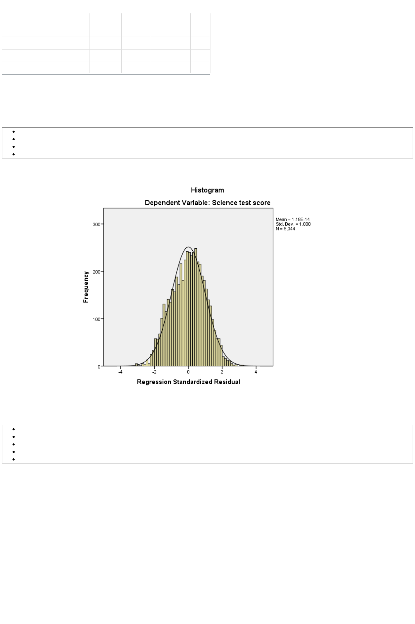
firstly plot a histogram of the residuals to check their normality which can be done in SPSS as follows:
Select Histogram from the Legacy diagnostics available from the Graphs menu.
Copy the Standardized Residual [ZRE_1] variable into the Variable box.
Click on the Display normal curve tick box.
Click on the OK button.
This will produce the graph as shown below:
Here we hope to see the histogram of residuals roughly following the shape of the normal curve that is superimposed over them.
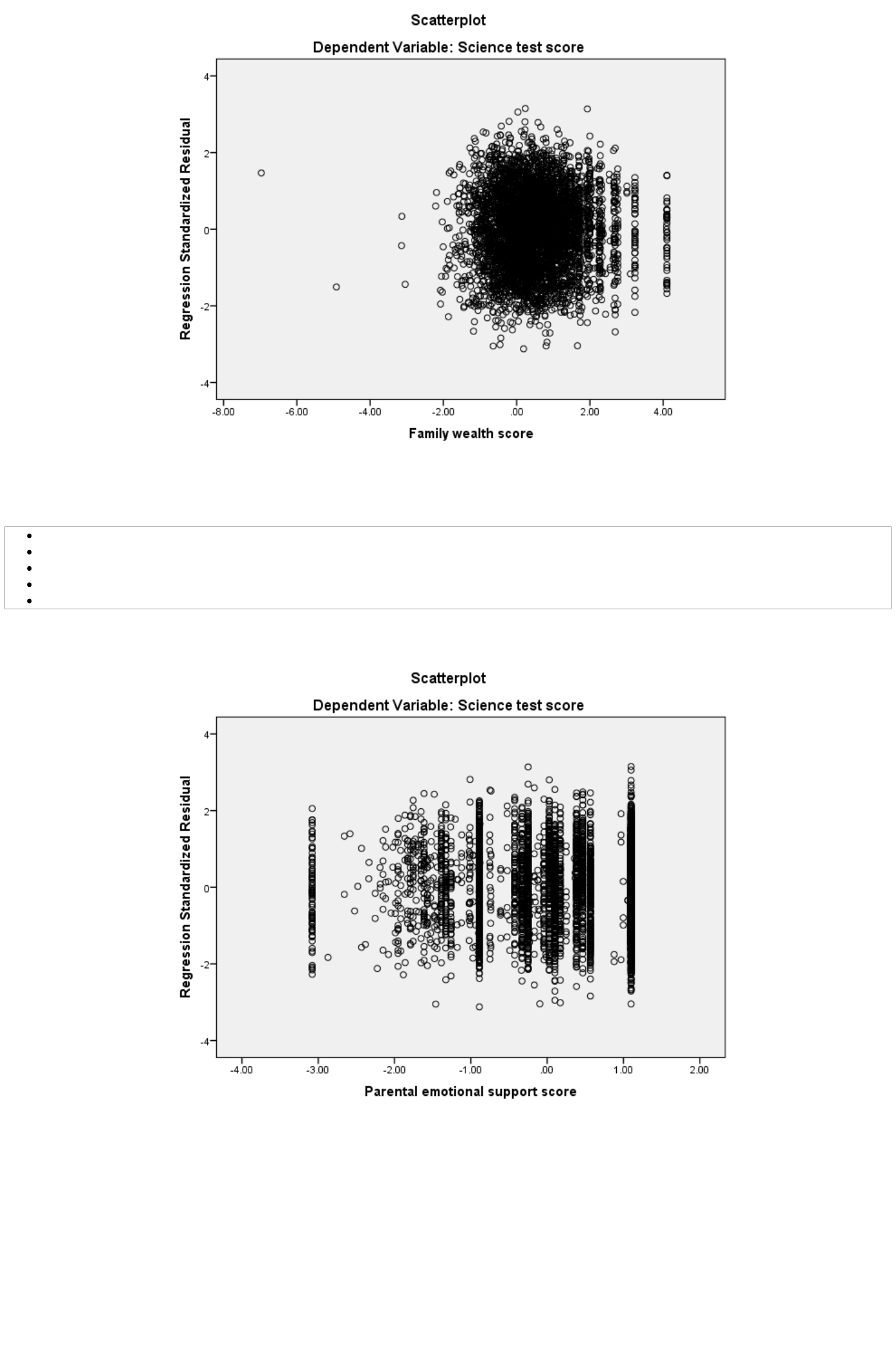
We can also look at how the distribution of the residuals interacts with the predictor variables in the model to check there is no
relationship. We do this via scatterplots which can be produced in SPSS as follows:
Select Scatter/Dot from the Legacy diagnostics available from the Graphs menu.
Select Simple Scatter and click on Define to bring up the Simple Scatterplot window.
Copy the Standardized Residual [ZRE_1] variable into the Y Axis box.
Copy the Family wealth score[WEALTH] variable into the X Axis box.
Click on the OK button.
This will produce the graph as shown below:
Here we have seen that parental wealth and parental emotional support are both significantly associated with a student’s science
achievement, and that each variable can independently predict the science test score when the other variable is held constant. The
conditional effect of emotional support is slightly stronger than that of wealth (a conclusion that comes from comparing the standardized
betas from the multiple regression) but, in total, these two predictors can only account for around 2 percent of the overall variation in test
scores.
Here we hope not to see any pattern where there was more variability in the residuals for particular values of Family wealth
score[WEALTH].
We can repeat this plot for Parental emotional support score[EMOSUPS] as follows:
Select Scatter/Dot from the Legacy diagnostics available from the Graphs menu.
Select Simple Scatter and click on Define to bring up the Simple Scatterplot window
Remove the Family wealth score[WEALTH] variable from the X Axis box.
Copy the Parental emotional support score[EMOSUPS] variable into the X Axis box.
Click on the OK button.
This will produce the graph as shown below:
Note that again we hope not to see any pattern in the residuals.
