Assessing the fiscal-monetary policy mix in the euro area

Working Paper Series

Assessing the fiscal-monetary

policy mix in the euro area

Krzysztof Bańkowski, Kai Christoffel,

Thomas Faria

Disclaimer: This paper should not be reported as representing the views of the European Central Bank

(ECB). The views expressed are those of the authors and do not necessarily reflect those of the ECB.

No 2623 / December 2021

Abstract

This paper attempts to gauge the eﬀects of various ﬁscal and monetary policy rules on

macroeconomic outcomes in the euro area. It consists of two major parts – a historical assessment

and an assessment based on an extended scenario until 2030 – and it builds on the ECB-BASE –

a semistructural model for the euro area. The historical analysis (until end-2019, ’pre-pandemic’)

demonstrates that a consistently countercyclical ﬁscal policy could have created a ﬁscal buﬀer

in good economic times and it would have been able to eliminate a large portion of the second

downturn in the euro area. In turn, the post-pandemic simulations until 2030 reveal that certain

combinations of policy rules can be particularly powerful in reaching favourable macroeconomic

outcomes (i.e. recovering pandemic output losses and bringing inﬂation close to the ECB target).

These consist of expansionary-for-longer ﬁscal policy, which maintains support for longer than

usually prescribed, and lower-for-longer monetary policy, which keeps the rates lower for longer

than stipulated by a standard reaction function of a central bank. Moreover, we demonstrate

that in the current macroeconomic situation, ﬁscal and monetary policies reinforce each other

and mutually create space for each other. This provides a strong case for coordination of the

two policies in this situation.

JEL classiﬁcation: E32, E62, E63

Keywords: Model simulations, Fiscal rules, Monetary policy rules, Joint analysis of ﬁscal and

monetary policy

ECB Working Paper Series No 2623 / December 2021

Non-technical Summary

Fiscal and monetary policy in the euro area exhibited distinct behaviours in the past, especially

amid the euro area sovereign debt crisis when ﬁscal policy was overall not supportive to growth (i.e.

procyclical). Against this background, this paper attempts to gauge the eﬀects of various ﬁscal and

monetary policy rules, irrespective of the existing institutional arrangements, on macroeconomic

outcomes under diﬀerent monetary policy rules. The analysis is conducted through the lens of

counterfactual scenarios using the ECB-BASE model, which is a semi-structural macroeconomic

model of the euro area.

In the model simulations we consider the two following subsamples: the historical pre-pandemic

period up to 2019Q4 and the post-pandemic projection period up to 2030. For the historical period

we mostly investigate whether diﬀerent ﬁscal policy behaviour – more aligned with the monetary

policy reaction – would have been able to improve stabilisation of the euro area economy compared

to the realised trajectories. We also carefully look how the eﬃciency and the cost of the alternative

ﬁscal policy arrangements depend on the reaction of the central bank. Turning to the post-pandemic

horizon, we note that this period is associated with great macroeconomic challenges such as low

natural interest rate and high government debt. Taking into account this environment, we attempt

to identify constellations of the two policies that would facilitate a strong performance of the euro

area economy going forward.

According to the model simulations for the historical period, consistently countercyclical ﬁscal

policy signiﬁcantly improves macroeconomic outcomes. In particular, it creates a buﬀer in good pre-

crisis times and, subsequently, eliminates a large portion of the second downturn associated with the

euro area sovereign debt crisis. Moreover, it noticeably reduces the negative inﬂation gap in recent

years. While these beneﬁts are attainable at a manageable cost, as judged by the debt-to-GDP ratio,

they are also conditional on monetary accommodation. Also importantly, the positive outcomes can

only be achieved if the alternative ﬁscal policy is implementable in the euro area in real time – an

aspect we do not assess in the paper.

Regarding the post-pandemic period, our analysis indicates that the combination of expansionary-

for-longer ﬁscal policy and low-for-longer monetary policy has a chance to signiﬁcantly improve

macroeconomic prospects. We deﬁne expansionary-for-longer ﬁscal policy as a policy that is ex-

ECB Working Paper Series No 2623 / December 2021

traordinarily cautious to ensure that a recovery is well in place and, as such, it maintains ﬁscal

support for longer and beyond the closure of the output gap. Low-for-longer monetary policy, in

turn, is deﬁned as a policy that keeps the rates lower for longer compared to what would be sug-

gested by the standard reaction function of a central bank. Concretely, this policy constellation

could recover around 50% of the accumulated output losses that materialised amid the pandemic

and bring inﬂation into the territory close to the ECB target. While admittedly, this policy course

would require a considerable ﬁscal expansion and it would lead to a non-negligible increase in gov-

ernment debt the euro area debt-to-GDP ratio would remain still on non-increasing path around

100%, for most policy mixes.

Our analysis also indicates, that at the current juncture ﬁscal and monetary policy reinforce each

other, pointing to complementarities between the two policies. Fiscal policy stimulates output and

inﬂation more under the low-for-longer monetary policy rule than under the standard Taylor rule.

In the same vein, the ability of monetary policy to positively inﬂuence macroeconomic conditions is

greater when ﬁscal policy is expansionary-for-longer rather than when ﬁscal policy behaves as it did

in the past. Another important ﬁnding of the model simulations is that both policies create mutual

space for each other. Fiscal policy alleviates the ELB constraint faced by monetary policy, thereby

empowering the central bank. On the other hand, monetary policy limits the cost of ﬁscal policy

by preserving favourable ﬁnancing conditions, hence it positively inﬂuences the ﬁscal space. This

provides a strong case for coordination between the two policies at the current juncture.

The stochastic simulations considering uncertainty conﬁrm the ﬁndings of the deterministic sim-

ulations. Moreover, these simulations assess the stabilisation properties of ﬁscal and monetary policy

in an optimistic growth scenario and a pessimistic growth scenario.

1 Introduction

The conduct of ﬁscal and monetary policy has changed notably in the EMU period. Until the

great ﬁnancial crisis (GFC) the aggregate variables representing the overall stance of policies (as

depicted by the euro area aggregate government budget balance and the ECB’s short-term interest

rate) co-moved with the business cycle (see Figure 1, co-movement with the output gap and the

inﬂation gap). In addition, in the wake of the GFC both policies strongly reacted to the downturn

ECB Working Paper Series No 2623 / December 2021

in a countercyclical fashion. Afterwards, however, a notable divergence between ﬁscal and monetary

policy emerged. While the latter, with the exception of a short tightening episode in 2011, kept

on progressing with an accommodative stance the former was tightening. In essence, ﬁscal and

monetary policy in the euro area reacted to the second downturn into opposite directions, with ﬁscal

policy exhibiting a procyclical stance.

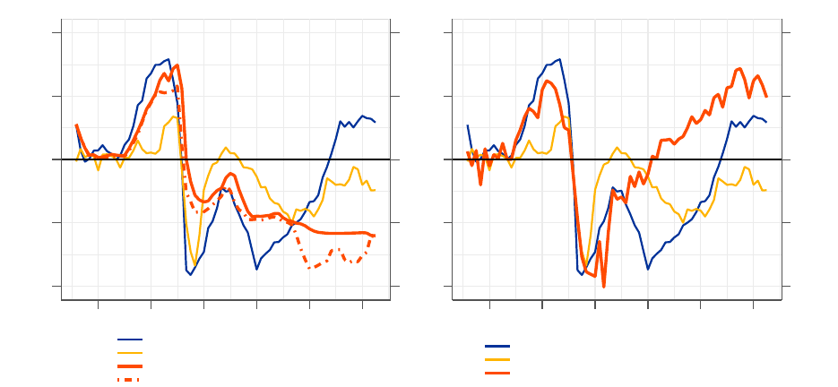
Figure 1: Policy reaction over the business cycle in the euro area

-4

-2

2004 2007 2010 2013 2016 2019

-4

-2

-7

-5

-3

-1

2004 2007 2010 2013 2016 2019

Output Gap (% of Pot. GDP)

Inﬂation Gap (pp)

Interest Rate (%, rhs)

Shadow Rate (%, rhs)

Output Gap (% of Pot. GDP)

Inﬂation Gap (pp)

Budget Balance (% of Pot. GDP, rhs)

Sources: Eurosystem and European Commission.

Notes: The inﬂation gap is calculated as the deviation to the 2% target value. The shadow rate is calculated according

to the methodology of Lemke and Vladu (2017). The potential GDP for the calculation of the output gap and the

budget balance-to-GDP ratio comes from the European Commission (Spring 2021 Economic Forecast) given that the

ECB does not publish potential GDP estimates.

The prevailing policy mix in the euro area since the formation of the EMU relied on monetary

policy as the main macroeconomic stabilisation tool. Fiscal policy instead was supposed to primarily

focus on ensuring debt sustainability and addressing country idiosyncratic shocks mostly by letting

automatic stabilisers operate freely. While the adequacy of this paradigm was largely unchallenged

during the great moderation period, the crisis episodes (i.e. the GFC and the COVID crisis) gave

rise to calls for a reassessment. Addressing these demands requires thorough analysis verifying to

which extent the policy mix in place was supportive to the achievement of the policy targets and

whether potential adjustments to the policy arrangements could improve the economic outcomes in

ECB Working Paper Series No 2623 / December 2021

the future.

A remarkable shift in the view on the role of ﬁscal policy in macroeconomic stabilisation has

materialised already in the aftermath of the GFC. In the policy realm a huge ’multiplier debate’

erupted in 2011 on the eﬀectiveness of ﬁscal policy after Olivier Blanchard – in his role as chief

economist of the International Monetary Fund – had emphasised that ﬁscal consolidations may be

self-defeating. The literature rediscovering the role of ﬁscal policies in macroeconomic stabilisation,

which simply burgeoned since then, pointed out mostly two key points (see Ramey (2019) for a

comprehensive literature survey). First, it underlined that at the lower bound ﬁscal policy is more

eﬀective than usual (see, e.g. Eggertsson (2011) and Christiano et al. (2011)). Second, it made

clear that ﬁscal policy might be indispensable for monetary policy to avoid persistent shortfalls of

inﬂation from its objective at the lower bound (see, e.g. Schmidt (2013) and Corsetti et al. (2019)).

Our paper aims to contribute to this strand of literature by conducting an empirical exercise for the

euro area. While many of the existing studies make use of parsimonious models to highlight key

mechanisms at play our paper aims to conduct the analysis in a realistic data-driven environment

that is closely linked to the prevailing macroeconomic conditions in the euro area (i.e. interest rates

at the ELB, subdued inﬂation staying persistently below the target and elevated government debt

levels).

This paper attempts to illustrate – through the means of counterfactual scenarios – the im-

plications of diﬀerent ﬁscal and monetary policy behaviours, captured by rules, for macroeconomic

outcomes.

To this end, we consider the historical pre-pandemic period up to 2019Q4 and a post-

pandemic projection period up to 2030. For the historical period we mostly investigate whether

ﬁscal policy that avoids procyclicality reduces cyclical ﬂuctuations. As far as the forward-looking

period is concerned, we attempt to identify constellations of policy rules that ensure favourable

macroeconomic outcomes (i.e. no negative output gap and no sizeable inﬂation shortfalls).

According to the model simulations, consistently countercyclical ﬁscal policy creates a buﬀer

in the good pre-GFC times and, subsequently, it has the potential to eliminate a large portion of

the second downturn associated with the euro area sovereign debt crisis. Moreover, it reduces the

Fiscal and monetary policy interact in multiple ways. Bassetto and Sargent (2020) emphasise that the separation

between the ﬁscal and monetary authority tends to be blurred. We maintain a clear separation of monetary and ﬁscal

authorities and analyse the interactions via the policy rules only.

ECB Working Paper Series No 2623 / December 2021

negative inﬂation gap in recent years without bringing large cost in terms of government debt. These

beneﬁts are conditional on full monetary accommodation.

Regarding the post-pandemic period, our analysis indicate that the combination of an expansionary-

for-longer ﬁscal policy (i.e. a policy that maintains ﬁscal support longer beyond the closure of the

standard output gap) and a low-for-longer monetary policy (i.e. a policy that keeps the rates low

for longer compared to a standard Taylor rule) has a chance to signiﬁcantly improve macroeconomic

prospects. Concretely, this policy constellation recovers around 50% of the accumulated output

losses that materialised amid the pandemic and brings inﬂation into the territory close to the ECB

target. Reaching such outcomes requires a moderate increase in government debt. Our analysis also

indicates that at the current juncture ﬁscal and monetary policy reinforce each other and mutually

create space for each other. This provides a strong case for the coordination between the two policies

currently.

We conduct our analysis in a rich macroeconomic environment and our ﬁndings illustrate how

conclusions of the academic literature on ﬁscal policy and its interactions with monetary policy can

be brought closer to policy-making. Most notably, we show that when the interest rate policy is

constrained − until 2024 in our case − ﬁscal policy becomes an eﬀective tool at the disposal of policy-

makers. While it is necessarily associated with budgetary costs, those are signiﬁcantly alleviated by

material beneﬁts to both real and nominal developments. This helps to reduce the tension between

the stabilisation needs and ﬁscal space when debt-to-GDP ratios are high (approaching 100% for

the euro area aggregate in the next years). Moreover and similarly to the literature ﬁndings, our

exercise shows that expansionary ﬁscal policy could support monetary policy. In particular, with

supportive ﬁscal policy, it would be easier to address the inﬂation shortfalls persisting in the euro

area rather than with monetary policy tools alone.

Due to the richness of the model speciﬁcation and the close link to the data, our analysis provides

a higher degree of realism in comparison to existing studies. Notwithstanding this, the modelling

exercise involves several limitations, which should have a bearing on the interpretation of the simula-

tion results. First, the euro area is modelled as a whole, thereby missing country heterogeneity and

other national aspects. This is particularly important because a desirable policy, even if identiﬁed,

may not be easily implementable given the incomplete setup of the ﬁscal architecture of the EMU.

ECB Working Paper Series No 2623 / December 2021

Moreover, it is virtually impossible at the aggregate level to reﬂect ﬁscal sustainability concerns of

the monetary union as these are driven by single member states. Second, the conducted exercise is

speciﬁc to the periods under consideration. For a general ranking of the policy rules, the analysis

should be re-conducted with stochastic simulations around the balanced growth path. Third, the

model does not feature sovereign default and it is therefore not suitable for sovereign stress analysis.

High debt-to-GDP ratios could increase the probability of sovereign stress in euro area Member

States, with a bearing on the cost of reﬁnancing. Fourth, the model is not equipped with a regime

switching to passive monetary policy and active ﬁscal policy and, as such, is not suitable for study-

ing ﬁscal dominance. Finally, the lack of model consistent expectations implies that agents in the

economy are not behaving in a Ricardian way. This could lead to an overestimation on the eﬃcacy

of ﬁscal policy for macroeconomic stabilisation, which is discussed in one of the subsections. In a

related vein, monetary policy cannot rely on the anticipation channel, dampening the eﬃcacy of

monetary policy tools.

The paper is structured as follows. Section 2 describes the model, with a focus on ﬁscal and

monetary policy rules. Section 3 and 4 contain the historical assessment and the post-pandemic

assessment respectively. Section 5 brieﬂy concludes.

2 Model set-up & speciﬁcation of the policy rules

The ECB-BASE is a semi-structural macroeconomic model of the euro area, developed for the use

in the macroeconomic projections, as well as for policy simulations (see Angelini et al. (2019) for a

model description). The model features a developed ﬁnancial block with elaborate monetary policy

channels. Also, the model is characterised by a rich representation of the general government, which

provides for a meaningful role of ﬁscal policy.

The applied version of the model embeds backward-looking expectations, which tilts the power

from monetary policy to ﬁscal policy compared to a DSGE model with forward-looking expect-

ations. Backward-looking expectations result in the absence of Ricardian equivalence.

In this

context, economic agents do not internalise any future consolidation needs resulting from a ﬁscal

In the situation of economic stress, like during the current COVID crisis, weakening the Ricardian equivalence

may be justiﬁed on the grounds that the share of liquidity constrained households is higher than usually.

ECB Working Paper Series No 2623 / December 2021

stimulus. Accounting for any anticipated future consolidation would weaken its eﬀects.

Similarly,

ﬁnancial market participants in the model are insensitive to any announced information on the fu-

ture developments in interest rates, or other monetary policy measures known in advance. This

eliminates the power of forward guidance that is present in DSGE models and weakens the potency

of monetary policy make-up rules, which largely work through anticipation channels (see Hebden

et al. (2020) for the analysis of the eﬀects of expectations on monetary policy make-up rules).

The quantitative responses of the ECB-BASE model to macroeconomic shocks are assessed in

Angelini et al. (2019) by benchmarking the model results against comparable models, including

semi-structural and DSGE models. One further reference for assessment can be found in the ’Basic

Model Elasticities’ (BMEs). These BMEs are developed by the National Banks of the Eurosystem

and are used regularly in the forecast exercises. They condense the views of modellers and forecasters

in the Eurosystem on the propagation of macroeconomic shocks.

To address a potential criticism

that the model gives too much power to ﬁscal policy and too little potency to monetary policy we

cross-check the eﬀects ﬁscal and monetary policy shocks with the BMEs as well. It turns out that

government spending multipliers are broadly consistent with those embedded in the BMEs and the

eﬀects of monetary policy are greater than according to the BMEs.

Based on this benchmarking

against reference models, we conclude that the power of the two policies is balanced.

One of the major advantages of the ECB-BASE model is its close link to the current conjunc-

tural developments. The model is ﬁrmly anchored not only in the historical data but also in the

Eurosystem projections. In particular, the baseline of the post-pandemic exercise reﬂects recent

macroeconomic projections.

As such, the model takes a comprehensive account of the current

The standard RBC/ NK model features inﬁnitely-lived households, whose consumption decisions at any point in

time are based on an intertemporal budget constraint. Ceteris paribus, an increase in government spending lowers

the present value of after-tax income, thus generating a negative wealth eﬀect that induces a cut in consumption.

In this context, standard macroeconomic models feature strong Ricardian eﬀects, which are sometimes at odds with

empirical ﬁndings (e.g. Blanchard and Perotti (2002)). Against this background, a vast amount of studies established

models, where the Ricardian eﬀects are weakened (see, for instance, Gali et al. (2007), which added rule-of-thumb

households).

The BMEs have been developed in the context of the Eurosystem projections and they summarise the eﬀects of

changes in assumptions (including ﬁscal and ﬁnancial assumptions) on macroeconomic variables. They can be inter-

preted as a simpliﬁed version of the macroeconomic models used by National Central Banks for economic projections.

As such, they constitute a benchmark for the assessment of ﬁscal and monetary policy in a macro model. ECB (2016)

provides details on BMEs and their application in the projections.

The comparison of policy eﬀects cannot be shown in this paper on account of the fact that the BME elasticities

are not made available to the public.

The baseline of the post-pandemic horizon exercise presented in the paper is broadly in line with the December

ECB Working Paper Series No 2623 / December 2021

environment with low interest rates, inﬂation persistently staying well below the target and large

negative output gaps amid the COVID crisis.

2.1 Baseline speciﬁcation of ﬁscal and monetary policy

With a view to comprehensively reﬂecting government accounts, ﬁscal policy in the ECB-BASE

involves multiple instruments. This applies to both the revenue and spending side of the budget.

Single instruments are in most of the cases modelled with Error Correction Mechanism (ECM)

equations appended with the output gap and deviations of the debt ratio from its target. These two

terms represent the stabilisation and sustainability components of ﬁscal policy.

In the context of this paper, the three following spending categories are used as primary ﬁscal

instruments: government transfers, purchases and investment.

The choice is motivated by the

observation that the changes in outlays within these items observed in the past were suﬃciently large

to inﬂuence the evolution of the output gap. This stands in contrast to, for instance, government

compensation which exhibits exceptionally stable dynamics in the data (see Figure A.1 in Appendix).

Moreover, all the three selected categories involve some characteristics of discretionary spending.

Given this we the three ﬁscal instruments as suitable for macroeconomic stabilisation purposes.

Speciﬁcally, the spending instruments considered in this paper evolve in line with Eq. 1. The

formula stipulates that actual spending (g

) converges towards its trend and, in addition, responds

to cyclical ﬂuctuations as well as to deviations of the debt-to-GDP ratio from its target.

∆g

= α



t−1

− g

t−1



+ δ∆g

k=1

∆g

t−k

+ γ



−



+ ε

(1)

where g

is log of actual spending, g

is log of trend spending,

is the real output gap,

the debt ratio to nominal output,

b is the debt-to-GDP ratio target and ε

is the residual term.

2020 macroeconomic projection (see ECB (2020) for the results), to the extent that macroeconomic variables are

made available to the public. The estimates of potential GDP, which are crucial for the analysis and which are not

published by the ECB, come from the European Commission’s Economic Forecast (Spring 2021).

To avoid complexity, we limit our investigation of ﬁscal rules to the spending side of the budget. In general,

government expenditures are characterised by a higher output multiplier compared to taxes as it aﬀects output more

directly. In this context, government spending may be seen as more suitable for output stabilisation than taxes.

Fiscal rules in the ECB-BASE are broadly consistent with those in DSGE models with elaborate ﬁscal policy (see,

for instance, Coenen et al. (2013)). In addition, the inclusion of trend and lags in the equation ensures a good data

ﬁt.

ECB Working Paper Series No 2623 / December 2021

The coeﬃcients entailed in the spending rules are estimated, summarising the average behaviour of

ﬁscal policy over the entire sample. This also applies to the coeﬃcient on the output gap, which

represents the cyclicality of ﬁscal policy. Given the contrasting nature of the euro area ﬁscal policy

(i.e. countercyclical amid the GFC and procyclical thereafter) the estimated coeﬃcients turn out to

be very small (see Table A.1 for exact values). This points to little reaction of ﬁscal policy to the

cycle on average embedded in the baseline ﬁscal rules.

Turning to monetary policy, the short-term interest rate follows a standard Taylor rule that

accounts for the ELB. The rule builds upon an empirical version of Taylor (1999), describing the

interest rate setting outside the constrained area.

= max

0.85R

t−1

+ 0.15



∗

+ ¯π

+ ( ¯π

− π

∗

)



, −0.5

+ ε

(2)

where R

denotes the nominal short term interest rate, r

∗

is the equilibrium real interest rate, ¯π

the average annual inﬂation rate, π

∗

denotes the 2% target, and

is the output gap.

The eﬀective

lower bound is imposed at -50 basis points.

In addition to the standard interest rate rule, the eﬀects of non-standard policies, in particular

asset purchases, are approximated via interest rate add-ons on short-term expectations and long-

term rates. This constitutes an indirect approach to account for the non-negligible eﬀects of APP

and PEPP on the risk premium and on expectations. To this end, the paper takes as given the

existing estimates of the eﬀect of quantitative easing on the yield curve (see Eser et al. (2019)). In

order to include these eﬀects into the simulation a simple rule is speciﬁed. This rule deﬁnes the

add-ons as a function of the inﬂation gap, that is only activated if interest rates are in negative

territory (see Eq. 3 and 4).

add,ST

= 0.99R

add,ST

+ 1 [R

≤ 0] 0.01 ( ¯π

− π

∗

) + ε

add,ST

(3)

add,LT

= 0.95R

add,LT

+ 1 [R

≤ 0] 0.05 ( ¯π

− π

∗

) + ε

add,LT

(4)

We base the values for the past unobserved natural rate in the euro area on Holston et al. (2017). Going forward

we assume that the value remains around zero as indicated by some of the estimates in Brand et al. (2018).

ECB Working Paper Series No 2623 / December 2021

Subsequently, these values are used to adjust the term premium of the long-term rates and VAR-

based expectation formation through the short-term rate. By incorporating into the analysis the

data on long-term interest rates, forward guidance is partly reﬂected in the baseline.

The analysis in this paper is based on the model under VAR expectations.

VAR expectations

assume only limited knowledge of the joint dynamics of the variables and they correspond to the

same restricted information set used in the estimation of the model. Speciﬁcally, the VARs share a

core set of macro variables: the policy rate, the GDP deﬂator, and the output gap. This design can

be interpreted as a limited form of rational expectations. The system of the core VAR variables is

augmented by the speciﬁc variable for which expectations are being formed. We label this form as

backward looking expectations because the information set for forming expectations is containing

only contemporaneous and past variables.

More precisely the setup of the VAR used for forming the expectations is:

∆z

= Λ

t−1

− z

∗

t−1

) +

k=1

∆z

t−k

(5)

where z

is a vector of variables containing inﬂation, the level of the interest rate and the output gap,

is a matrix containing coeﬃcients that control how the variables respond to the deviation of the

lagged level from the long-term attractors, Λ

are matrices that collect autoregressive coeﬃcients for

K lags. There are two diﬀerent cases how expectations enter into the model. For the price and wage

equations the expectations of the t + h-quarter variable is based on rolling the VAR forward. For

variables inside the PAC speciﬁcation, the VAR deﬁnes the information set to map into the desired

level of the target variable.

Backward-looking expectations of the model do not allow for analysing the eﬀects of forward guidance in a

commensurate way.

Similarly to the FRB/US model, the ECB-BASE can technically allow for two alternative ways of forming the

expectations of diﬀerent agents. Speciﬁcally, expectations can be either based on projections from an estimated

small-scale auxiliary VAR model (i.e. VAR or limited information expectations) or consistent with a full knowledge

of the dynamics of the model (i.e model-consistent or rational expectations). The latter case assumes that agents

are fully rational and their expectations are based on the solution of the model under the assumption that also the

expected variables follow the internal logic of the model. Rational expectations are sometimes criticised as being overly

optimistic on the assumption that agents have a complete understanding of the economy and base their expectation

on this understanding.

Angelini et al. (2019) contains an in-depth description of the expectation formation process in the ECB-BASE.

ECB Working Paper Series No 2623 / December 2021

2.2 Alternative ﬁscal policy and monetary policy rules

We deﬁne the rule with the estimated coeﬃcients as the baseline, which turns out to be broadly

neutral (i.e. acyclical) to the cycle. A ﬁrst counterfactual rule is then deﬁned as a rule that decisively

reacts to real economic developments in a countercyclical fashion. Such a rule has its natural limit,

once the real output gap closure is achieved. After deep recessions with lasting inﬂation shortfalls,

it might still be warranted to keep ﬁscal stimulus in place. To address this limitation we introduce

further rules based on an augmented output gap, which deviates from the standard gap only when the

policy rate hits the ZLB. We label rules of this type as expansionary-for-longer ﬁscal policy because

they provide ﬁscal support for longer, beyond the point when the output gap closes. Such ﬁscal

policy rules constitute an analogy to low-for-longer monetary policy rules, which provide monetary

support beyond what is suggested by a standard Taylor rule.

The exact speciﬁcation of the countercyclical ﬁscal rules is as follows (see Eq. 6).

∆g

= α



t−1

− g

t−1



+ δ∆g

k=1

∆g

t−k

+ γ



−



+ ε

(6)

where γ

<< 0. In fact, what makes the countercyclical ﬁscal rule distinct from an estimated ﬁscal

rule (see Eq. 1) is the size of the coeﬃcient on the output gap, which in the case of the latter is

close to zero.

The ﬁrst approach to implement expansionary-for-longer ﬁscal policy is based on the substitution

of the real output gap by the nominal output gap – the nominal approach. This means that the real

output gap is augmented by a price gap, computed as cumulative inﬂation deviations over time. The

second approach relies on augmenting the standard output gap with past negative output gaps – the

real approach. This implies that policy-makers rather than being concerned only about closing the

contemporanous output gap attempt to also compensate additionally for past output shortfalls.

There are multiple reasons for ﬁscal policy to consider not only the real but also the nominal

Given the complexity of the spending rules the interpretation of γ

may not be straight-forward. The value used

in the analysis for government purchases is equal to -0.1 which is a value that ensures a sizeable, albeit still plausible,

ﬁscal expansion (see Figure 13 for the exact amounts of additional expenditure associated with various scenarios).

The coeﬃcient values for other instruments (i.e. social transfers and government investment) are rescaled accordingly

so that a ﬁscal expansion is evenly distributed across the three instruments used in the analysis.

This might be considered in cases where protracted shortfalls lead to hysteresis or scarring eﬀects which are not

fully reﬂected in the level of the output gap.

ECB Working Paper Series No 2623 / December 2021

developments in policy setting. First, nominal income, and not only real income, is a relevant

variable perceived by economic agents, thereby constituting the basis for their business decision

making. Second, it is nominal income that is relevant for debt sustainability – one of the main

concerns for a ﬁscal authority. Third, the price dynamics embedded in the nominal concept may

improve the understanding of the current state of the business cycle given material uncertainty about

the unobservable real output gap (see for example Jarociński and Lenza (2018)). Finally, a ﬁscal

authority responding only to real developments and the monetary authority reacting solely to price

dynamics may result in the divergence of policy courses. The aim to coordinate, will necessarily

involve policy rules based on similar variables (i.e. see, for instance, Bianchi et al. (2020) suggesting

a common strategy for ﬁscal and monetary policy in the current environment).

Importantly, such a formulation does not call for any shift of responsibility between monetary

and ﬁscal authorities. With policy rates at the ELB monetary policy may not be able to ensure

adequate dynamics on the nominal side. In such a situation ﬁscal policy, supported by favourable

ﬁnancing conditions, remains an eﬀective macroeconomic tool. In a situation characterised by a

closed output gap and still subdued price dynamics, nominal output gap targeting on the ﬁscal side

could contribute to excess demand and higher prices simultanously. It would deliver some make-up

for the large output losses experienced in the euro area both during the great recession and amid

the COVID crisis.

Turning to the real approach, expansionary-for-longer ﬁscal policy can also be achieved by con-

sidering past negative real output gaps when the interest rate is at the ZLB. This speciﬁcation can

be mostly motivated by the desire to recover at least some of the signiﬁcant output losses that

materialised during severe crises (e.g. amid the GFC or the COVID crisis). Our model baseline

indicates that cumulative output losses with respect to potential GDP are reaching around 15%

of GDP, which is undeniably a sizeable ﬁgure (see Figure 5). The case for recovering past output

losses is particularly strong in the presence of hysteresis eﬀects, which stipulates that grave output

shortfalls aﬀect potential GDP.

In such an environment, a period of excess demand could help to

address some of these adverse eﬀects, thereby preserving potential capacity of the economy. This

Permanent damage to a potential output following a cyclical recession can materialise through a number of

channels such as labour force, capital stock and productivity. Cerra et al. (2020) contains a review of the related

literature.

ECB Working Paper Series No 2623 / December 2021

may be the case currently when the COVID crisis brings massive disruptions to economic activity.

Formally, the expansionary-for-longer ﬁscal rules can be described by the following equation

∆g

= α



t−1

− g

t−1



+ δ∆g

k=1

∆g

t−k

+ γ

aug,i

+ γ



−



+ ε

(7)

where γ

<< 0 remains like in the countercyclical ﬁscal rules. The speciﬁcation of

aug,i

depends

on whether we consider the nominal (i = nom; see Eq. 8) or the real (i = real; see Eq. 9) approach.

It is crucial to emphasise that the augmenting terms, which cumulate the inﬂation deviations in

the case of

or output shortfalls in the case of

add

embed a memory loss (see the details on

Appendix Section B). Varying the degree of it is useful to demonstrate how expansionary-for-longer

ﬁscal policy gains strength in macroeconomic stabilisation.

aug,nom

+ 1 [R

≤ 0]

(8)

aug,real

+ 1 [R

≤ 0]

add

(9)

Turning to monetary policy, the paper considers three alternative policy rules which embed

various degrees of monetary accommodation. These rules stipulate average inﬂation targeting with

an averaging windows of diﬀerent length. As such, the rules take into account the accumulated

inﬂation deviations over the corresponding time windows. Given the persisting negative inﬂation

deviations, the rules imply additional monetary accommodation (i.e. keeping rates low for longer)

compared to the standard Taylor rule at the current juncture.

For this reason, we label the regimes

implied by these alternative rules as low-for-longer monetary policy.

Concretely, the rules feature inﬂation gaps based on 2-year, 3-year and 4-year averaging windows.

The speciﬁcation of the rules is consistent with the study by Arias et al. (2020) prepared for the

IMF (2021) points to signiﬁcant scarring eﬀects to global output in the medium term as a result of the pandemic.

Without any memory loss the price gap becomes very large given the persistent inﬂation shortfalls in recent years.

The large size makes the gap hardly usable as an indicator in a policy rule.

The readiness of a policy-maker to cool the economy because of a realised inﬂation overshooting may be diﬀerent

from the readiness to stimulate the economy because of realised inﬂation shortfalls. To reﬂect this, some studies,

like Arias et al. (2020), consider asymmetric average inﬂation rules, where the make-up strategy only applies to past

inﬂation shortfalls. In our analysis this is the case even with the symmetric rules because the inﬂation have been

recording negative deviations in the data.

ECB Working Paper Series No 2623 / December 2021

discussion of the Federal Reserve’s review of monetary policy strategy.

Formally the rule for a

T-year average inﬂation targeting follows Eq. 10 with ¯π

(T −year )

being the T-year average inﬂation.

= max

0.85R

t−1

+ 0.15



∗

+ ¯π

+ T



¯π

(T −year )

− π

∗



, −0.5

+ ε

(10)

2.3 Criteria for assessing the rules

Having speciﬁed ﬁscal and monetary policy rules for the analysis it is equally important to lay out

criteria used for their assessment. By contrast to many papers in the academic literature, we do not

attempt to identify optimal rules for ﬁscal and monetary policy (see Benigno and Woodford (2003))

for a single economy and Kirsanova et al. (2007) for a monetary union as examples of studies).

Instead, we consider rules that are commonly accepted in the policy-making world and extend them

along several dimensions as explained in Subsection 2.2. The modiﬁcations are motivated by the

desire to improve realised or projected macroeconomic outcomes, such as high output volatility or

persisting inﬂation shortfalls.

In contrast to the existing literature based on parsimonious theoretical models, we do not assess

the rules with a single welfare-based loss function (see the derivation for a simple NK model in Gali

(2015)). ECB-BASE is not rigorously micro-founded and consequently, does not feature an explicit

welfare measure. Specifying a loss function in this context would necessarily require additional

assumptions, such as weighting the typical loss function variables.

We focus, instead, on a set of variables that are relevant to policy-makers and will allow them to

judge the rules with a cost-beneﬁt approach. In line with the chosen policy rules, we use output gap

and inﬂation. In addition to this we analyse the policy variables themselves and variables that are

informative about the cost of stabilisation. For monetary policy, these are the short-term interest

rate and the ZLB duration. For ﬁscal policy, these are the budget balance-to-GDP ratio and the

government debt-to-GDP ratio. To condense the ﬁndings of the simulations we do not only oﬀer

graphical presentation of the above mentioned variables but also summarise them in heat maps for

The average inﬂation targeting rules in Arias et al. (2020) rely on 4-year and 8-year averaging windows. We

consider shorter horizons for the sake of realism.

Hauptmeier and Kamps (2020), for instance, in their assessment of selected ﬁscal rules assume that a ﬁscal

authority follows a quadratic loss function consisting of the output gap and government debt-to-GDP deviations. The

aggregation of the two terms requires choosing υ parameter (where 0 < υ < 1), which represents the preference of a

ﬁscal authority to stabilise the business cycle relative to debt sustainability.

ECB Working Paper Series No 2623 / December 2021

the post-pandemic scenario (see Figure 11, 12 and 13.)

3 Historical perspective

The analysis of ﬁscal policy in this section is based on counterfactual scenarios conducted around

the historical sample from 2003 to 2019. Through the lens of the ECB-BASE model we attempt to

illustrate how various ﬁscal policies aﬀect the business cycle under two diﬀerent conﬁgurations of

monetary policy.

The ﬁrst set of simulations assumes that monetary policy does not react to any

changes brought by the alteration of the ﬁscal rules and remains the same as observed in the data. In

the second step, the monetary policy reaction becomes endogenous with the central bank following a

standard Taylor rule. Eventually, by turning to stochastic simulations we generalise the illustration

by considering uncertainty. The analysis remains agnostic on whether the ﬁscal policy implied by

the considered ﬁscal rules was implementable given past ﬁnancial and political conditions.

3.1 Fiscal rules with exogenous monetary policy

According to the model simulations, the alternative ﬁscal rules substantially smooth the real out-

put gap and slightly reduce the inﬂation gap without causing a surge in the government debt. A

systematically countercyclical policy (see Figure 2, Countercyclical rule) reduces the output gap

ﬂuctuations signiﬁcantly. Initially, the spending retrenchment imposed by the rule during the good

pre-crisis times dampens the positive output gap noticeably. Afterwards, a supportive ﬁscal policy

that sharply reacts to the downturns facilitates the post-GFC recovery and alleviates the gravity of

the second downturn. While the inﬂation beneﬁts are non-negligible during the post-GFC period,

the inﬂation rate still remains far from the target for an extended period of time given the large size

of the recorded shortfalls.

Scenarios with expansionary-for-longer ﬁscal rules (see Figure 2, Expansionary-for-longer I, II,

III rules) bring additional stimulating eﬀects. The countercyclical ﬁscal rule that reacts to the

standard output gap stops providing support with the output gap closure in late 2016. This is the

moment when the expansionary-for-longer ﬁscal policy starts making a sizeable diﬀerence providing

One crucial assumption underlying the simulations is that all shocks/ residuals in the model remain unchanged

compared to those associated with the realised data.

ECB Working Paper Series No 2623 / December 2021

support beyond the output gap closure. Fiscal policy under these rules constitutes an option to

further diminish the accumulated output losses amid the two crisis episodes or to support inﬂation

dynamics. This, however, requires a prolongation of the ﬁscal stimulus well beyond the sovereign

debt crisis, which is associated with a considerable overheating of the economy in recent years. In

fact, the implementation of the expansionary-for-longer rules more than overcompensates for the

accumulated output losses towards the end of the sample with inﬂation still not being ﬁrmly on

target.

Judging by the evolution of the debt-to-GDP ratio in the various scenarios, sizeable beneﬁts of

expansionary-for-longer ﬁscal policy come at only limited cost under the assumption of full monetary

accommodation. Increases in debt as a share of potential GDP associated with the alternative ﬁscal

policies are small. The investigated ﬁscal rules ﬁrst lead to savings prior to the GFC, thereby building

a small ﬁscal buﬀer. Afterwards, supportive ﬁscal policies, even the expansionary-for-longer versions,

yield substantial beneﬁts to both real and nominal sides, which signiﬁcantly alleviates the cost of the

increased expenditures. With policy rates being unresponsive, monetary policy keeps the servicing

cost of the sovereigns debt low. It also provides an additional accommodation, in the sense of

keeping rates unchanged against the background of higher output and inﬂation. The ﬁndings of

the simulations heavily rely on the assumption that policy-makers know in real time the current

estimates of the output gap and are able to adjust policies accordingly. Given the extent of the

revisions to the output gap, accurate ﬁscal policy ﬁne-tuning is very diﬃcult in practice.

ECB Working Paper Series No 2623 / December 2021

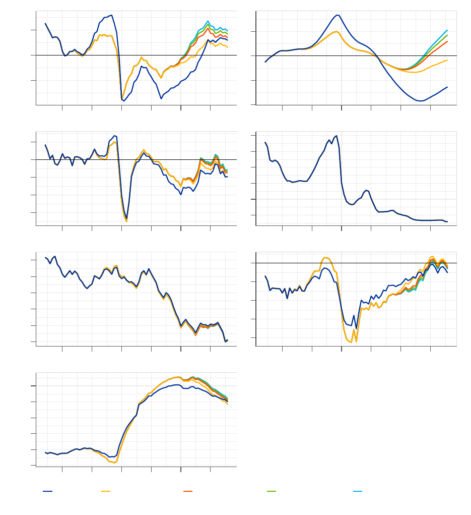
Figure 2: Historical counterfactual simulations of various ﬁscal rules with exogenous monetary policy

-2

2003 2006 2009 2012 2015 2018

Output Gap (% of Pot. GDP)

-10

-5

2003 2006 2009 2012 2015 2018

Cum. Output Loss wrt 02Q1 (% of Pot. GDP)

-1

2003 2006 2009 2012 2015 2018

Inﬂation (%)

2003 2006 2009 2012 2015 2018

Interest Rate (%)

2003 2006 2009 2012 2015 2018

10Y long-term rate (%)

-8

-6

-4

-2

2003 2006 2009 2012 2015 2018

Budget Balance (% of Pot.

GDP)

2003 2006 2009 2012 2015 2018

Gov. Debt (% of P

ot. GDP)

Estimated Countercyclical Exp.-for-longer I Exp.-for-longer II Exp.-for-longer III

Sources: ECB-BASE simulations.

Notes: "Estimated" ﬁscal rule reproduces the observed data. The expansionary-for-longer ﬁscal rules presented in

the context of the historical exercise are formulated on the basis of the nominal approach. Rules bringing equivalent

outcomes can be devised following the real approach (see the demonstration for the post-pandemic horizon, Subsection

4.2).

ECB Working Paper Series No 2623 / December 2021

3.2 Fiscal rules with endogenous monetary policy

The sizeable macroeconomic eﬀects of ﬁscal policy in Subsection 3.1 are conditional on fully accom-

modative monetary policy. The assumption of exogenous monetary policy implies that the central

bank undertakes the same measures as observed in the past irrespective of inﬂation and output gap

outcomes. Relaxing this assumption, namely that the central bank reacts to more positive macroe-

conomic outcomes brought by an alternative ﬁscal policy (for instance, by following a Taylor rule)

may be seen as more realistic and it changes the picture materially.

The simulations indicate that for the eﬃcacy of ﬁscal rules full accommodation of monetary

policy is crucial. In a conﬁguration with endogenous monetary policy, the central bank responds

to the macroeconomic developments according to the Taylor rule. Prior to the GFC, the policy

rate in the simulations remains below the baseline. Subsequently, given the improved economic

conditions, the rate is above baseline and remains there also during the second downturn. The

monetary policy reaction has substantial consequences for the eﬃcacy of the investigated ﬁscal rules

in our simulations. More concretely, the extent to which ﬁscal policy reduces output gap ﬂuctuations

is more limited compared to the case with full monetary accommodation (see Figure 3). None of

the ﬁscal rules eliminates the crisis-related accumulated output losses at the end of the simulation

horizon. Moreover, virtually no gains from the alternative ﬁscal policy rules are visible for inﬂation.

With ﬁscal support in place the monetary policy rate reaches the ELB signiﬁcantly later than

in the data (i.e. in late 2017 rather than in mid-2015). In this context, the alternative ﬁscal rules

create ample room for monetary policy. The expansionary-for-longer ﬁscal rules start making a

diﬀerence only during the last part of the simulation period. This is because the activation of

the augmented gap is conditional on the central bank being at the ZLB (see the explanations in

Subsection 2.2). In this context, there are no substantial changes to government expenditure and

no material implications for economic outcomes compared to the countercyclical rule.

Endogenous monetary policy also aﬀects the size of ﬁscal cost of the alternative ﬁscal rules. Prior

to the crisis, interest rates are lower than observed in the data, therefore contributing to the build-up

of a ﬁscal buﬀer. Following the GFC this tendency is reverting, however. The less accommodative

stance of monetary policy gradually increases the servicing cost of government debt. This, together

with additional expenditure and limited macroeconomic beneﬁts, brings the debt-to-GDP ratio to

ECB Working Paper Series No 2623 / December 2021

levels noticeably exceeding the observed values.

ECB Working Paper Series No 2623 / December 2021

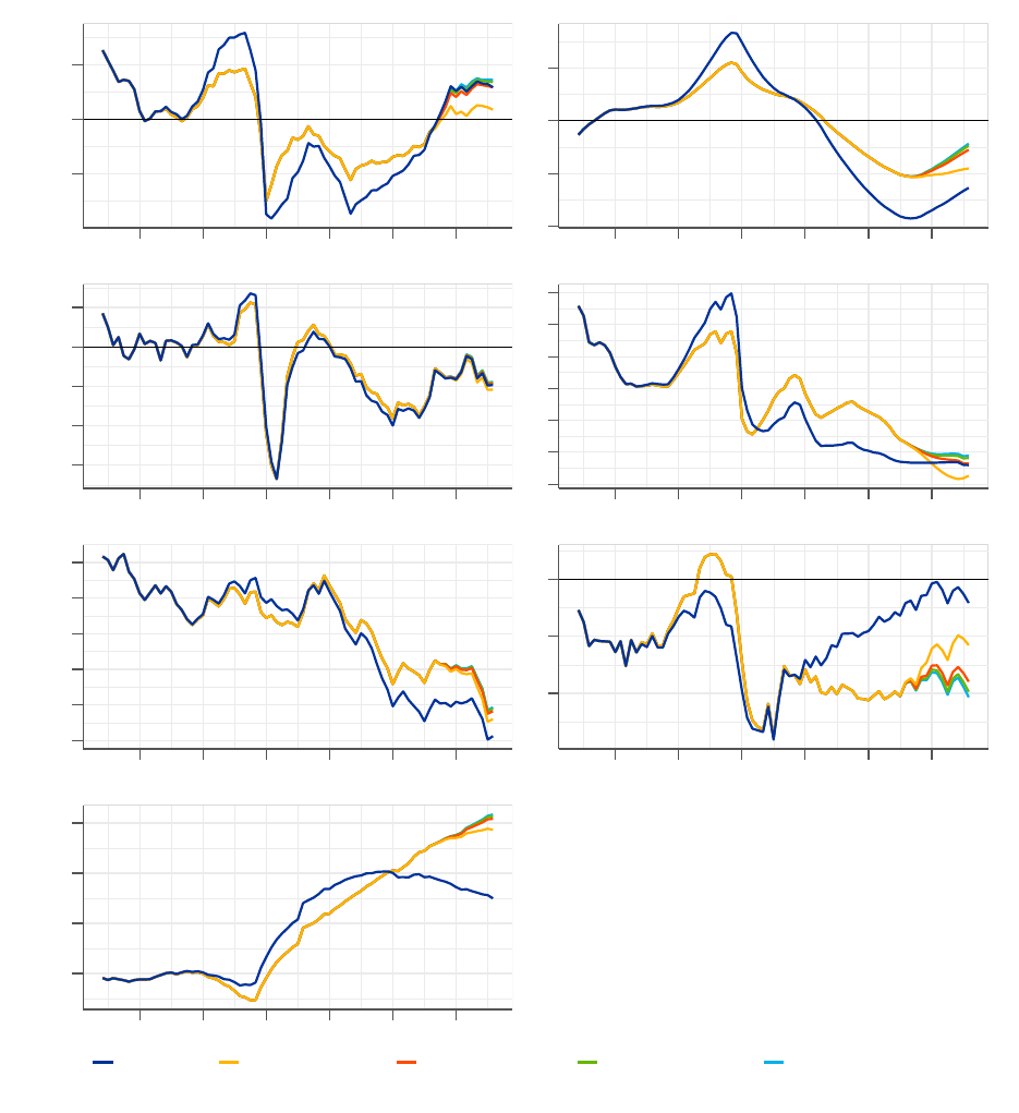
Figure 3: Historical counterfactual simulations of various ﬁscal rules with endogenous monetary

policy following a standard Taylor rule

-2

2003 2006 2009 2012 2015 2018

Output Gap (% of Pot.

GDP)

-10

-5

2003 2006 2009 2012 2015 2018

Cum. Output Loss wrt 02Q1 (%

of Pot. GDP)

-1

2003 2006 2009 2012 2015 2018

Inﬂation (%)

-1

2003 2006 2009 2012 2015 2018

Interest Rate (%)

2003 2006 2009 2012 2015 2018

10Y long-term rate (%)

-5.0

-2.5

0.0

2003 2006 2009 2012 2015 2018

Budget Balance (% of Pot. GDP)

100

2003 2006 2009 2012 2015 2018

Gov. Debt (% of Pot. GDP)

Estimated Countercyclical Exp.-for-longer I Exp.-for-longer II Exp.-for-longer III

Sources: ECB-BASE simulations.

Notes: "Estimated" ﬁscal rule reproduces the observed data. The expansionary-for-longer ﬁscal rules presented in

the context of the historical exercise are formulated on the basis of the nominal approach. Rules bringing equivalent

outcomes can be devised following the real approach (see the demonstration for the post-pandemic horizon, Subsection

4.2).

ECB Working Paper Series No 2623 / December 2021

The deterministic simulation presented hitherto evaluate the policy mix in a ceteris paribus

environment assuming that all shocks and residuals remain at the values identiﬁed by inverting

the baseline model. One way to evaluate the robustness of the results is to conduct stochastic

simulations. By drawing from model residuals and repeating the simulations multiple times the

analysis incorporates the eﬀects of uncertainty and possible model misspeciﬁcations.

The depicted

means of the stochastic distributions under the counterfactual policy experiments show a picture

consistent with the counterfactual scenarios described above (see Figure 4; more details on stochastic

simulations, including the occurrences of risk events, is given in Section 4). The diﬀerences between

stochastic means across various scenarios very much resemble those of the deterministic simulations.

The property that the means of the stochastic simulations are situated below the deterministic

simulation is due to existence of the ELB. For those paths, where the interest rate is constrained by

the ELB, particularly negative paths for output and inﬂation are more frequently observed. This

induces a negative bias in the distribution of output and inﬂation. Non-standard monetary policy

dampens the negative outcomes but it cannot fully compensate for the lack of the interest rate

instrument during ELB episodes. In this environment, alternative ﬁscal rules improve the outcomes

signiﬁcantly when it comes to the output gap (see Figure 4, the diﬀerence between the blue/ yellow

lines and the other lines) and inﬂation.

The residuals of the equations capture the part of the observed variables that cannot be explained by the structure

of the equations.

ECB Working Paper Series No 2623 / December 2021

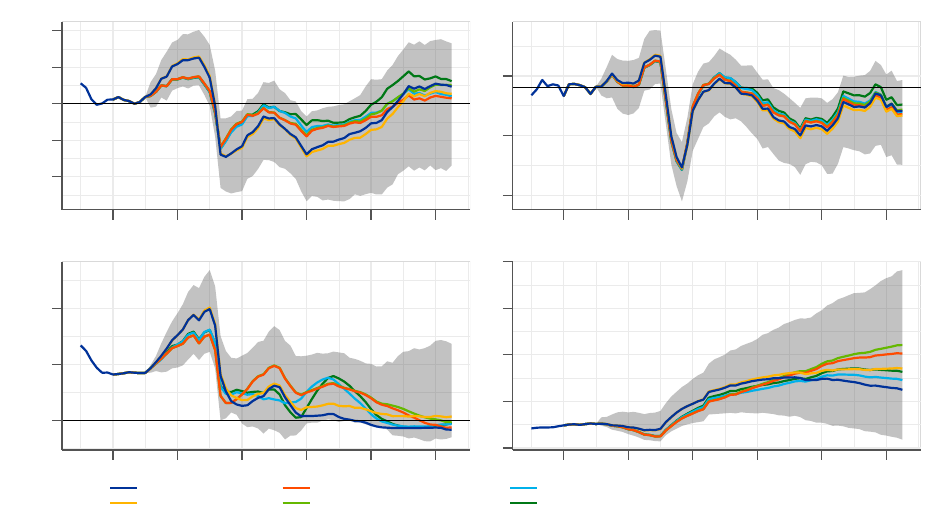
Figure 4: Stochastic simulations of various ﬁscal and monetary policy rules

-5.0

-2.5

0.0

2.5

5.0

2004 2007 2010 2013 2016 2019

Output Gap (% of Pot. GDP)

-2.5

0.0

2.5

2004 2007 2010 2013 2016 2019

Inﬂation (%)

0.0

2.5

5.0

2004 2007 2010 2013 2016 2019

Interest Rate (%)

100

120

140

2004 2007 2010 2013 2016 2019

Gov. Debt (% of Pot. GDP)

Baseline

TR & Estimated

TR & Countercyclical

TR & Exp.-for-longer II

Low-for-longer II & Coun

tercyclical

Low-for-longer III &

Exp.-for-longer III

Sources: ECB-BASE simulations.

Notes: The conﬁdence bands are based on stochastic simulations with the baseline policy rules. The bands are based

on 2.5% and 97.5% percentiles. The alternative rules are presented by the mean of the stochastic simulations to

maintain readability.

4 Post-pandemic perspective

By conducting simulations over an extended horizon until 2030, we investigate how diﬀerent con-

ﬁgurations of ﬁscal and monetary policy aﬀect the expected medium-term macroeconomic outlook.

The starting point for the exercise is the construction of a reference baseline with ﬁscal and monet-

ary policy rules that are consistent with the existing institutional arrangements and the dynamics

observed in the past (i.e. the estimated ﬁscal rules and the Taylor rule speciﬁed in Subsection 2.1).

Subsequently, we vary the rules (for both ﬁscal and monetary policy) and assess how their diﬀerent

combinations perform relative to the baseline.

The reference baseline is broadly consistent with the Eurosystem projections (the December 2020

exercise, see ECB (2020) for the results). We complement the set of projected variables published

ECB Working Paper Series No 2623 / December 2021

by the ECB, which does not include the potential output, with the potential output of the European

Commission. The projected variables are reproduced by the model until the end of their forecast

horizon (i.e. end-2023 for the Eurosystem and end-2022 for the European Commission). Afterwards

the ﬁgures are model-based.

To construct post-2023 baseline we use information contained in the model residuals. Rather

than imposing zero residuals in the calculations the residual in-sample information is considered.

Speciﬁcally, it is assumed that residuals consist of a systematic and idiosyncratic component. The

former is derived from an auxiliary state space model and used for the post-2023 simulation (the

appendix of Angelini et al. (2019) contains a description of the methodology). This approach greatly

improves the realism of the medium-term baseline compared to the approach based on zero residuals.

In the baseline the output gap is nearly closed already within the Eurosystem forecast horizon

and remains close to zero thereafter (see Figure 5). The narrowing of the inﬂation gap with respect

to the 2% target occurs at signiﬁcantly lower speed in comparison to the closure of the output gap.

The short-term interest rate remains at the ELB until the end of the Eurosystem forecast horizon

and then lifts oﬀ following the Taylor rule. Public ﬁnances normalise gradually, following the grave

consequences of the COVID crisis. Speciﬁcally, the budget balance-to-GDP ratio converges towards

a balanced position and the debt-to-GDP ratio starts falling, albeit from an elevated level.

ECB Working Paper Series No 2623 / December 2021

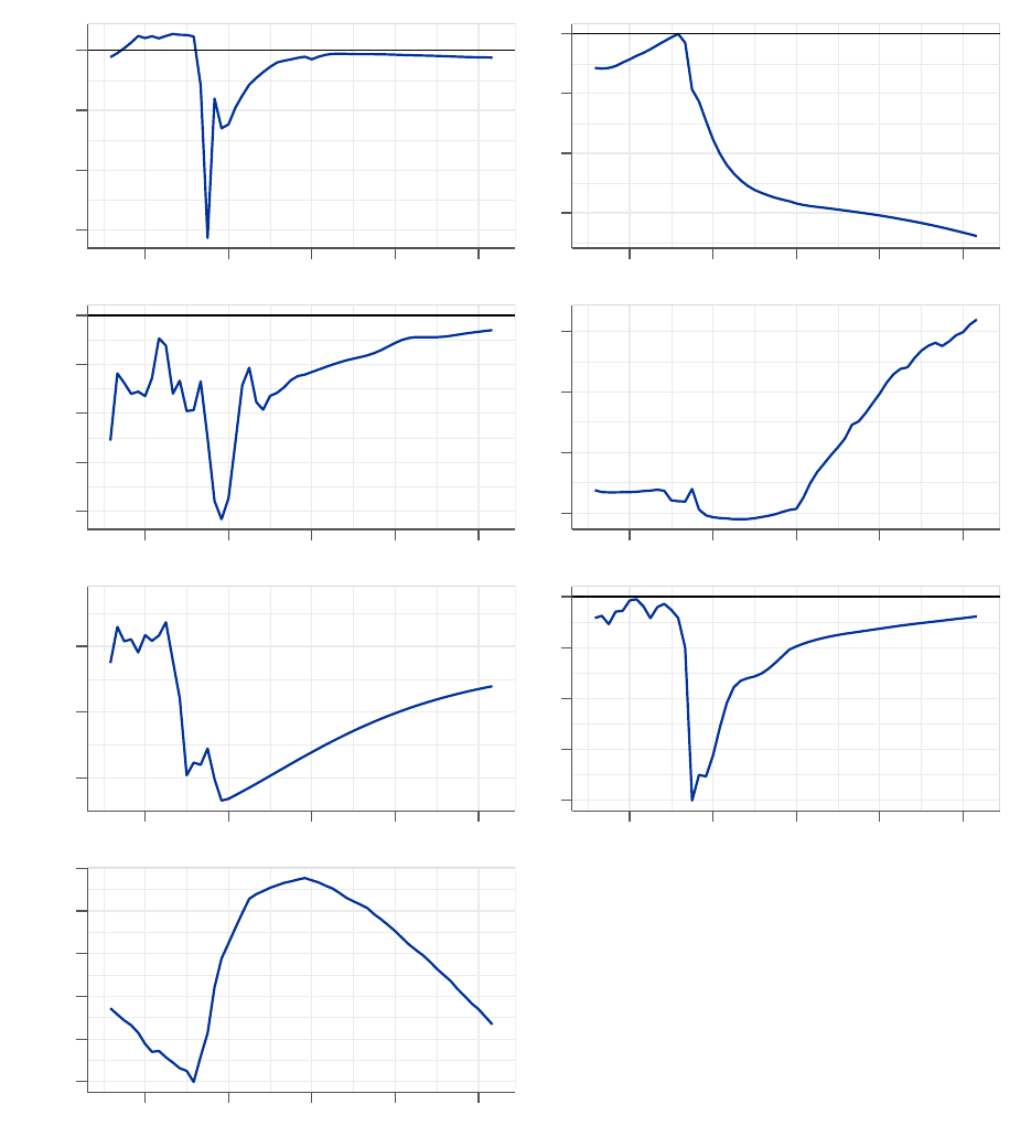
Figure 5: Medium-term reference baseline

-15

-10

-5

2018 2021 2024 2027 2030

Output Gap (% of Pot. GDP)

-15

-10

-5

2018 2021 2024 2027 2030

Cum. Output Loss wrt 19Q4 (% of Pot. GDP)

0.0

0.5

1.0

1.5

2.0

2018 2021 2024 2027 2030

Inﬂation (%)

-0.5

0.0

0.5

1.0

2018 2021 2024 2027 2030

Interest Rate (%)

0.0

0.5

1.0

2018 2021 2024 2027 2030

10Y long-term rate (%)

-10.0

-7.5

-5.0

-2.5

0.0

2018 2021 2024 2027 2030

Budget Balance (% of Pot.

GDP)

85.0

87.5

90.0

92.5

95.0

97.5

2018 2021 2024 2027 2030

Gov. Debt (% of P

ot. GDP)

Sources: ECB-BASE simulations.

Notes: The baseline presented above is broadly consistent with the Eurosystem projections for the variables that are

made available to the public (see ECB (2020)). The output gap, which is not published, is based on the potential

output of the European Commission (Spring 2021 Economic Forecast). In the post-forecast period the ﬁgures are

model-based.

ECB Working Paper Series No 2623 / December 2021

4.1 Fiscal and monetary policy rules in isolation

Before analysing combinations of the rules, we look at the eﬀects of ﬁscal and monetary policy rules

in isolation. This means that a change to ﬁscal rules and its macroeconomic consequences will be

ignored by monetary policy (i.e. monetary policy is exogenous and kept at its baseline values).

Similarly, when analysing monetary policy rules, we assume no reaction from the side of ﬁscal policy

(i.e. ﬁscal policy exogenous). While this set-up is hardly realistic it helps to understand the economic

impact of ﬁscal and monetary policy alone without mixing the policies and their eﬀects.

Fiscal policy rules can signiﬁcantly alter the macroeconomic outcomes compared to the baseline.

In particular, a countercyclical ﬁscal policy stimulates output leading to a very fast output gap

closure and it lifts inﬂation by a non-negligible margin (see Figure 6). The expansionary-for-longer

ﬁscal rules bring inﬂation back to target still within the projection horizon. At the same time, they

signiﬁcantly reduce the cumulative output gap losses. This involves, however, a sizeable amount

of additional stimulus compared to the baseline as indicated by the deterioration in the budget

balance. Moreover, it also necessitates the tolerance of overheating the euro area economy (output

gap reaching 2% of GDP in the coming years). While the additional stimulus does increase the

debt-to-GDP ratio in a few years’ time it does not raise it in the medium term in 2030.

ECB Working Paper Series No 2623 / December 2021

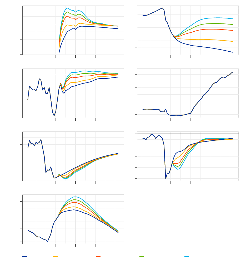
Figure 6: Post-pandemic simulations of various ﬁscal policy rules in isolation.

-4

-2

2018 2021 2024 2027 2030

Output Gap (% of Pot. GDP)

-15

-10

-5

2018 2021 2024 2027 2030

Cum. Output Loss wrt 19Q4 (% of Pot. GDP)

0.0

0.5

1.0

1.5

2.0

2018 2021 2024 2027 2030

Inﬂation (%)

-0.5

0.0

0.5

1.0

2018 2021 2024 2027 2030

Interest Rate (%)

0.0

0.5

1.0

2018 2021 2024 2027 2030

10Y long-term rate (%)

-10.0

-7.5

-5.0

-2.5

0.0

2018 2021 2024 2027 2030

Budget Balance (% of Pot.

GDP)

100

2018 2021 2024 2027 2030

Gov. Debt (% of P

ot. GDP)

Estimated Countercyclical Exp.-for-longer I Exp.-for-longer II Exp.-for-longer III

Sources: ECB-BASE simulations.

Notes: "Estimated" ﬁscal rule reproduces the reference baseline presented in Figure 5.

ECB Working Paper Series No 2623 / December 2021

Model simulations also reveal that interest rate rules can alter the expected paths for macroeco-

nomic variables, albeit only to a limited extend.

Both real output and inﬂation improve slightly

with more accommodative monetary policy rules (see Figure 7). The reason for limited gains lies in

the limited monetary policy space in the baseline. In this context, the additional rules that we con-

sider make a relatively small diﬀerence. The short-term interest rate in the outer years is lower only

by a maximum of around 0.7 percentage point. Furthermore, with backward-looking expectations

in the model there is no expectation channel of monetary policy. In contrast to forward-looking

models, only the realised changes in interest rates matter but not the expected path of interest rates

in the future. In the simulations, the non-standard monetary policy is modelled through add-ons

(see the description in Subsection 2.1) which are kept endogenous. For a complete assessment of the

role of monetary policy, the impact of forward guidance would need to be included.

The investigation of monetary policy rules in isolation involves shutting down the reaction of ﬁscal policy. This

still involves an active ﬁscal block (i.e. no exogenisation of the entire ﬁscal block). In particular, changes in tax

bases translate into corresponding changes in tax revenue. Moreover, all ﬁscal identities, including the budget balance

and debt accumulation remain fully operational. In practice, shutting down the reaction of ﬁscal policy does not

materially change the outcomes compared to the estimated ﬁscal rules, which embed very little reaction to the cycle

(as discussed in Subsection 2.1).

ECB Working Paper Series No 2623 / December 2021

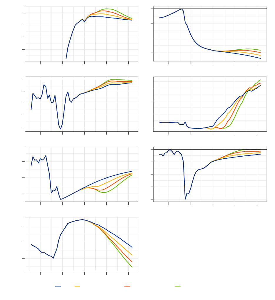
Figure 7: Post-pandemic simulations of various monetary policy rules in isolation

-3

-2

-1

2018 2021 2024 2027 2030

Output Gap (% of Pot. GDP)

-15

-10

-5

2018 2021 2024 2027 2030

Cum. Output Loss wrt 19Q4 (% of Pot. GDP)

0.0

0.5

1.0

1.5

2.0

2018 2021 2024 2027 2030

Inﬂation (%)

-0.5

0.0

0.5

1.0

2018 2021 2024 2027 2030

Interest Rate (%)

0.0

0.5

1.0

2018 2021 2024 2027 2030

10Y long-term rate (%)

-10.0

-7.5

-5.0

-2.5

0.0

2018 2021 2024 2027 2030

Budget Balance (% of Pot.

GDP)

2018 2021 2024 2027 2030

Gov. Debt (% of P

ot. GDP)

TR Low-for-longer I Low-for-longer II Low-for-longer III

Sources: ECB-BASE simulations.

Notes: "TR" monetary rule reproduces the reference baseline presented in Figure 5.

ECB Working Paper Series No 2623 / December 2021

4.2 Combinations of ﬁscal and monetary policy rules

To have a realistic assessment of the eﬀectiveness of the two policies we run simulations under

endogenous ﬁscal and monetary rules. We start with the analysis of various ﬁscal rules where the

monetary policy reacts in a usual manner following a standard Taylor rule.

The gains from ﬁscal policy rules combined with a standard monetary policy reaction, that is not

providing any further accommodation, are limited. While alternative ﬁscal rules initially provide a

signiﬁcant boost to real activity and to prices the eﬀect is short-lived (see Figure 8). This is because

the standard Taylor rule promptly reacts to the macroeconomic improvements. As such, the beneﬁts

of ﬁscal policy are eliminated by an ‘uncooperative’ monetary policy tightening. Furthermore,

interest rate increases lead to a situation in which the governments face higher ﬁnancing costs, which

gradually propagate into the overall debt servicing cost. This brings detrimental consequences for

the debt-to-GDP ratio and makes the ﬁscal policy very costly.

ECB Working Paper Series No 2623 / December 2021

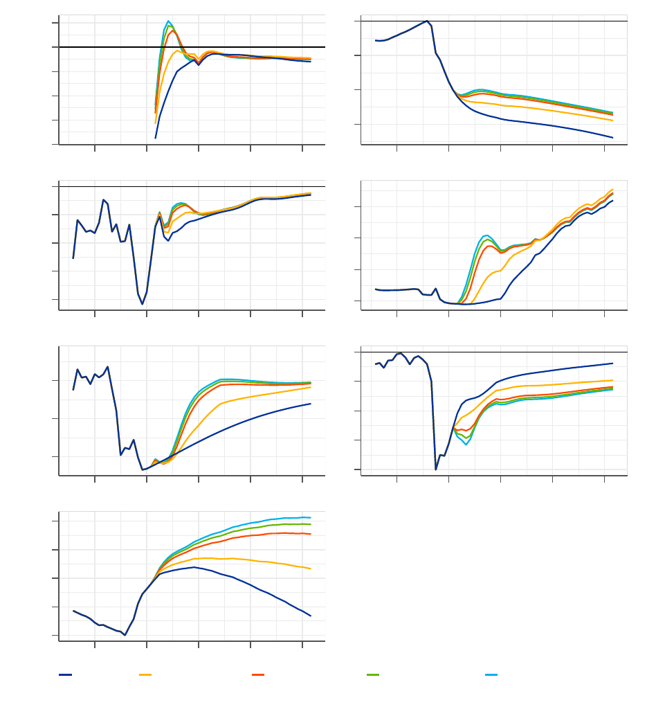
Figure 8: Post-pandemic simulations of various ﬁscal rules with endogenous monetary policy follow-

ing the standard Taylor rule

-4

-3

-2

-1

2018 2021 2024 2027 2030

Output Gap (% of Pot.

GDP)

-15

-10

-5

2018 2021 2024 2027 2030

Cum. Output Loss wrt 19Q4 (%

of Pot. GDP)

0.0

0.5

1.0

1.5

2.0

2018 2021 2024 2027 2030

Inﬂation (%)

-0.5

0.0

0.5

1.0

2018 2021 2024 2027 2030

Interest Rate (%)

0.0

0.5

1.0

2018 2021 2024 2027 2030

10Y long-term rate (%)

-10.0

-7.5

-5.0

-2.5

0.0

2018 2021 2024 2027 2030

Budget Balance (% of Pot. GDP)

100

105

2018 2021 2024 2027 2030

Gov. Debt (% of Pot. GDP)

Estimated Countercyclical Exp.-for-longer I Exp.-for-longer II Exp.-for-longer III

Sources: ECB-BASE simulations.

Notes: "Estimated" ﬁscal rule reproduces the reference baseline presented in Figure 5.

ECB Working Paper Series No 2623 / December 2021

To uncap the potential of ﬁscal policy, more accommodative monetary policy rules are essential.

With monetary policy still reacting but working in concert with ﬁscal policy the macroeconomic

beneﬁts are signiﬁcantly more tangible.

Fiscal policy can provide a signiﬁcant boost to output

and inﬂation when monetary policy delivers additional accommodation in parallel (see Figure 9 and

10). In our illustration, monetary policy, in contrast to the standard Taylor rule reaction, does

not ﬁght back the beneﬁts of ﬁscal policy but rather tries to create favourable conditions for it by

lifting the rates only gradually. This makes the macroeconomic gains of ﬁscal policy sizeable and

long-lasting. However, only with a considerable additional spending and signiﬁcant overheating of

the economy, a combination of expansionary-for-longer ﬁscal policy and low-for-longer monetary

policy has a chance to bring inﬂation close to the 2% target during the simulation horizon. This

scenario halves the output losses accumulated amid the COVID crisis. Also, no sharp monetary

policy tightening means no abrupt increases of the ﬁnancing cost for the governments. This makes

the application of ﬁscal policy signiﬁcantly less costly compared to the situation in which the central

bank strictly follows the standard Taylor rule.

Both formulations of expansionary-for-longer ﬁscal policy (i.e nominal and real approach) bring

virtually the same macroeconomic outcomes (compare Figure 9 and Figure 10). In this context, a

ﬁscal authority does not need to choose between the two speciﬁcations. Rather it needs to make a

choice how to communicate an expansionary-for-longer ﬁscal policy. The nominal-based speciﬁcation

explicitly acknowledges the role of ﬁscal policy in reaching the inﬂation target at the time when the

central bank is constrained. The real-based speciﬁcation emphasises the objective to recover some of

the output losses. At the current juncture both aims coincide and require the same course of ﬁscal

policy.

The lack of any monetary policy reaction could be interpreted as a case of subordination of monetary policy to

the needs of ﬁscal policy or ﬁscal dominance. In the analysis we do not consider this theoretical constellation as it

remains at odds with the prevailing institutional arrangement.

ECB Working Paper Series No 2623 / December 2021

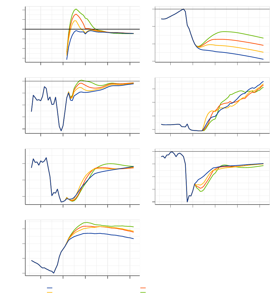
Figure 9: Post-pandemic simulations of ﬁscal and monetary policy rules working in concert

(expansionary-for-longer ﬁscal policy speciﬁed following the nominal approach)

-3

-2

-1

2018 2021 2024 2027 2030

Output Gap (% of Pot.

GDP)

-15

-10

-5

2018 2021 2024 2027 2030

Cum. Output Loss wrt 19Q4 (%

of Pot. GDP)

0.0

0.5

1.0

1.5

2.0

2018 2021 2024 2027 2030

Inﬂation (%)

-0.5

0.0

0.5

1.0

2018 2021 2024 2027 2030

Interest Rate (%)

0.0

0.5

1.0

2018 2021 2024 2027 2030

10Y long-term rate (%)

-10.0

-7.5

-5.0

-2.5

0.0

2018 2021 2024 2027 2030

Budget Balance (% of Pot. GDP)

100

2018 2021 2024 2027 2030

Gov. Debt (% of Pot. GDP)

TR & Countercyclical

Low-for-longer I & Exp.-for-longer

Low-for-longer II & Exp.-for-longer II

Low-for-longer III &

Exp.-for-longer III

Sources: ECB-BASE simulations.

ECB Working Paper Series No 2623 / December 2021

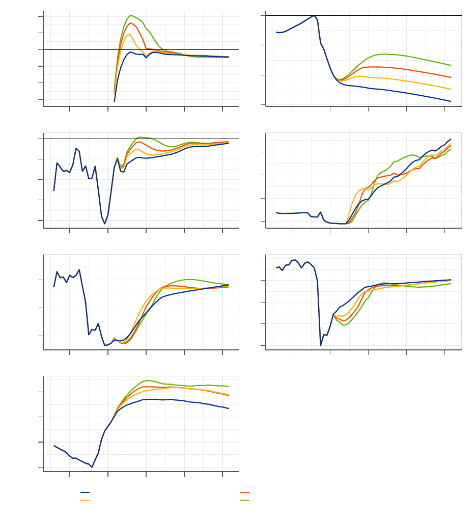
Figure 10: Post-pandemic simulations of ﬁscal and monetary policy combinations working in concert

(expansionary-for-longer ﬁscal policy speciﬁed following the real approach)

-3

-2

-1

2018 2021 2024 2027 2030

Output Gap (% of Pot.

GDP)

-15

-10

-5

2018 2021 2024 2027 2030

Cum. Output Loss wrt 19Q4 (%

of Pot. GDP)

0.0

0.5

1.0

1.5

2.0

2018 2021 2024 2027 2030

Inﬂation (%)

-0.5

0.0

0.5

1.0

2018 2021 2024 2027 2030

Interest Rate (%)

0.0

0.5

1.0

2018 2021 2024 2027 2030

10Y long-term rate (%)

-10.0

-7.5

-5.0

-2.5

0.0

2018 2021 2024 2027 2030

Budget Balance (% of Pot. GDP)

100

2018 2021 2024 2027 2030

Gov. Debt (% of Pot. GDP)

TR & Countercyclical

Low-for-longer I & Exp.-for-longer

Low-for-longer II & Exp.-for-longer II

Low-for-longer III &

Exp.-for-longer III

Sources: ECB-BASE simulations.

ECB Working Paper Series No 2623 / December 2021

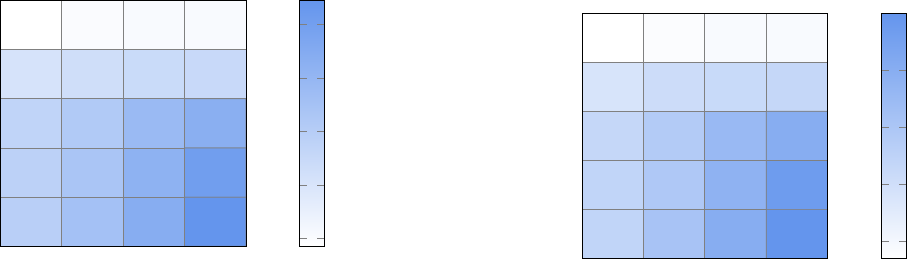
Figure 11: The eﬀects of various combinations of ﬁscal and monetary rules on output gap and

inﬂation

(a) Output gap

(% of GDP, 2021q3-25q4 average)

w-for-longer I

Low-for-longer I

Estimated

Countercyclical

Exp.-for-longer I

Exp.-for-longer II

Exp.-for-longer III

−1.06 −1 −0.98 −0.98

−0.58 −0.49 −0.43 −0.41

−0.32 −0.14

0.13 0.32

−0.27 −0.06

0.27 0.61

−0.23

0.01 0.36 0.78

Monetary Policy

Fiscal Policy

−1

−0.6

−0.2

0.2

0.6

(b) Inﬂation

(%, 2021q3-25q4 average)

w-for-longer I

Low-for-longer II

w-for-longer III

Estimated

Countercyclical

Exp.-for-longer I

Exp.-for-longer II

Exp.-for-longer III

1.37 1.38 1.39 1.39

1.48 1.51 1.52 1.53

1.53 1.58 1.65 1.7

1.54 1.59 1.68 1.77

1.54 1.61 1.7 1.8

Monetary Policy

Fiscal Policy

1.4

1.5

1.6

1.7

1.8

Sources: ECB-BASE simulations.

Notes: The intersection of the estimated ﬁscal rule (Estimated) and the Taylor monetary policy rule (TR) corres-

ponds to the baseline. Comparing the outcomes to the baseline is a way to assess the eﬀectiveness of various policy

constellations.

A more detailed look at all simulation scenarios reveals that monetary policy uncaps the potential

of ﬁscal policy. The more accommodative monetary policy is, the higher are the output gains

associated with ﬁscal rules (see Figure 11, subﬁgure (a), vertical gains are bigger for Expansionary-

for-longer III scenario compared to TR scenario). The positive average output gap of 0.8% of GDP

associated with the most favourable policies compares to -1.1% of GDP in the baseline and implies

around 8% of additional output by end-2025. This addresses the large cumulative output losses that

arose amid the COVID crisis. Similarly, inﬂation beneﬁts most from the alternative ﬁscal rules under

the most accommodative monetary policy arrangement (see Figure 11, subﬁgure (b)). Concretely,

while the average inﬂation can beneﬁt from the most expansionary-for-longer ﬁscal policy by less

than 0.2 percentage points under the Taylor rule arrangement the gains exceed 0.4 percentage points

under the most accommodative low-for-longer monetary policy. With this outcome the inﬂation

reaches 1.8% on average, which is closest to the target among all constellations we consider in our

analysis.

ECB Working Paper Series No 2623 / December 2021

It is not only that monetary policy uncaps the potential of ﬁscal policy but also ﬁscal policy

makes monetary policy more powerful. While the potency of monetary policy in the absence of

expansionary-for-longer ﬁscal policies is relatively limited (see Figure 11, subﬁgures (a) and (b)

horizontal gains of the ﬁrst row) under the assumption of expansionary-for-longer ﬁscal policy mon-

etary policy can still noticeably increase output and inﬂation (see Figure 11, subﬁgures (a) and (b),

horizontal gains of the last row). This occurs because ﬁscal policy with its power to stimulate the

economy alleviates the ELB and creates space for additional interest rate stimulus.

The model simulations suggest that the largest increases in output and inﬂation can be obtained

when both ﬁscal and monetary policy work hand in hand. Looking at the heatmaps summarising the

results, it becomes apparent that adjusting both policies simultaneously brings the biggest beneﬁts

(see Figure 11, subﬁgures (a) and (b), gains by moving along a diagonal towards the right lower

corner). None of the policies on its own can perform so well. Against this background, ﬁscal and

monetary policy reinforce each other and exhibit the properties of complementarity.

Another conclusion brought by the model simulations is that both policies mutually create space

for each other. In particular, ﬁscal policy can alleviate some of the burden placed on monetary policy.

With the expansionary-for-longer ﬁscal policy the interest rates are on average higher compared to

the estimated ﬁscal rule (see Figure 12, subﬁgure (a)). This leads to a situation in which the central

bank is able to lift the interest rate earlier than in the baseline. The exit from the undesirable ZLB

environment materialises in 2023-24 rather than in 2026-27 (see Figure 12, subﬁgure (b)).

ECB Working Paper Series No 2623 / December 2021

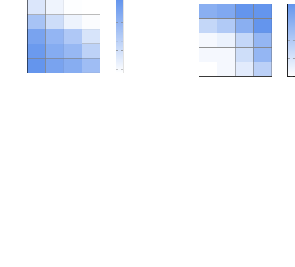
Figure 12: The eﬀects of various combinations of ﬁscal and monetary rules on the short-term interest

rate and the timing of the ZLB exit

(a) Short-term interest rate

(%, 2021q3-25q4 average)

w-for-longer I

w-for-longer II

Low-for-longer I

Estimated

Countercyclical

Exp.-for-longer I

Exp.-for-longer II

Exp.-for-longer III

−0.36 −0.46 −0.53 −0.54

−0.1 −0.29 −0.45 −0.52

0.13 0

−0.14 −0.34

0.2 0.07

−0.02 −0.21

0.24 0.13 0.06

−0.06

Monetary Policy

Fiscal Policy

−0.5

−0.4

−0.3

−0.2

−0.1

0.1

0.2

(b) Timing of the ZLB exit

(year during which the rate becomes positive)

w-for-longer I

Low-for-longer I

w-for-longer III

Estimated

Countercyclical

Exp.-for-longer I

Exp.-for-longer II

Exp.-for-longer III

2026 2026 2027 2027

2024 2025 2026 2027

2023 2023 2024 2025

2023 2023 2023 2024

Monetary Policy

Fiscal Policy

2023

2024

2025

2026

2027

Sources: ECB-BASE simulations.

Notes: The intersection of the estimated ﬁscal rule (Estimated) and the Taylor monetary policy rule (TR) corres-

ponds to the baseline. Comparing the outcomes to the baseline is a way to assess the eﬀectiveness of various policy

constellations.

In the same vein, monetary policy creates space for ﬁscal policy, which takes place through two

mechanisms in the model. First, accommodative monetary policy does not ﬁght back the positive

eﬀects of ﬁscal stimuli and, as such, it allows the budget to beneﬁt from the improved macroeconomic

conditions. Second, by holding back interest rate increases the central back ensures favourable

ﬁnancing conditions for the government, thereby eﬀectively keeping the cost of debt servicing in

check. In the model simulations, the increase in debt-to-GDP ratio under the most accommodative

low-for-longer monetary policy is smaller than under the Taylor rule (see Figure 13, subﬁgure (b)).

This occurs even though the amount of additional expenditure is noticeably higher (see Figure 13,

subﬁgure (a)).

The result that the ﬁscal expansion under the low-for-longer monetary policy is more sizeable than under the

Taylor rule regime relates to the set-up of the expansionary-for-longer ﬁscal policy rules (see Subsection 2.2). The

expansionary-for-longer ﬁscal rules, by deﬁnition, only make a diﬀerence if interest rates are negative. Under low-for-

longer monetary policy the central banks holds back with interest rate increases, which extends the duration of the

ZLB period and makes the extraordinary support embedded in the expansionary-for-longer ﬁscal policy activated.

ECB Working Paper Series No 2623 / December 2021

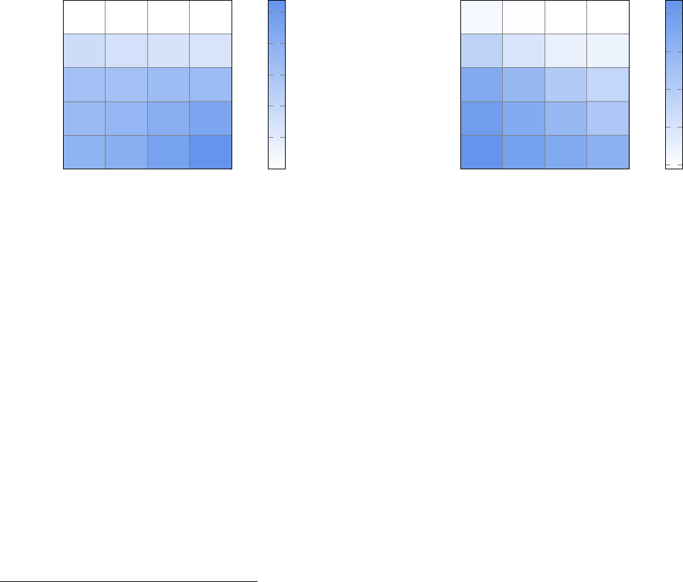
Figure 13: The eﬀects of various combinations of ﬁscal and monetary rules on the primary expendit-

ure and the government debt

(a) Additional primary spending relative to the baseline

(% of GDP, cumulated over 2021q3-25q4)

w-for-longer I

w-for-longer II

Low-for-longer I

Estimated

Countercyclical

Exp.-for-longer I

Exp.-for-longer II

Exp.-for-longer III

0 0 0 0

3.4 3 2.8 2.7

6.2 6.4 6.7 6.9

7 7.3 8.2 8.9

7.6 8.1 9.3 10.7

Monetary Policy

Fiscal Policy

(b) Government debt-to-GDP ratio for analysed scenarios

(%, end-2025q4)

w-for-longer I

w-for-longer II

Low-for-longer I

Estimated

Countercyclical

Exp.-for-longer I

Exp.-for-longer II

Exp.-for-longer III

95.4 95 94.8 94.8

98.5 97 96.1 95.8

101.9 100.7 99.2 98.1

102.9 101.8 100.8 99.5

103.7 102.7 101.9 101.3

Monetary Policy

Fiscal Policy

101

103

Sources: ECB-BASE simulations.

Notes: The intersection of the estimated ﬁscal rule (Estimated) and the Taylor monetary policy rule (TR) corres-

ponds to the baseline. Comparing the outcomes to the baseline is a way to assess the eﬀectiveness of various policy

constellations.

The extension of the baseline until 2030, underlying the above discussed simulations, is based on

a number of assumptions and it is subject to uncertainty. The stochastic simulations allow to assess

uncertainty and its eﬀects on the baseline and on the counterfactual simulations.

Stochastic simulations also allow to conduct risk analysis through the occurrence of undesirable

events, from the point of view of monetary or ﬁscal policy. We deﬁne these events as hitting the

ELB, low inﬂation episodes, enduring deep recessions or recording high debt-to-GDP ratios.

Table

1 shows the frequency of these events for the two subsamples under consideration. In both cases,

the introduction of the alternative ﬁscal and monetary rules has an impact on the frequency of

See also the description of the stochastic simulations in Section 3. The model for the stochastic simulations diﬀers

slightly from the model in the deterministic simulations. First, an ELB at -50bp is introduced also for the long-term

rate to avoid negative realisations of long-term rates in the lower part of the distribution. Second, in the baseline and

deterministic simulations, the asset purchases are calibrated taken into account APP and PEPP (Pandemic emergency

purchase program). For the stochastic simulation the calibration was slightly reduced to tone down the eﬀects of asset

purchases for the general case without PEPP.

The incidences of risk events are derived by calculating the number of simulation points inside the stochastic

distribution where a certain deﬁned event is fulﬁlled, and relating this number to the total number of simulation

points.

ECB Working Paper Series No 2623 / December 2021

occurrences of these risk events. Comparing the two subsamples shows that the number of ELB

incidences under the baseline speciﬁcation in the historical period is signiﬁcantly lower than during

the post-pandemic horizon. The diﬀerences are driven by the respective levels of interest rates in

the two samples, where higher interest rate levels make ELB events less likely. While the historical

sample starts from relatively high interest rates, the extended horizon is initiated at the ELB. A

similar argument holds for the occurrence of high debt events, which are more likely in the second

sample, because the initial debt level is already elevated. In comparison to the baseline with the

estimated ﬁscal rules and the Taylor rule, the introduction of the countercyclical ﬁscal policy makes

the adverse events, with the exception of high debt, less likely. The negative impact on debt is

related to the fact that the lack of coordination with monetary policy makes a ﬁscal stimulus more

costly. Once monetary policy becomes more accommodative (i.e. see low-for-longer policy rules) the

high debt incidence goes down in both subsamples. Introducing the low-for-longer monetary policy

rules, however, without adjusting ﬁscal policy results in an increase of the ELB occurrence, because

the ELB episodes are longer. The frequency of ELB episodes is reduced in the post-pandemic sample

when ﬁscal policy provides an additional stimulus.

A qualitative diﬀerence between the two samples relates to the occurrence of high debt incidences.

While in the historical sample the combination of expansionary-for-longer ﬁscal policy and low-for-

longer monetary policy is reducing the incidence frequencies for high debt, the opposite is true in

the extended scenario. Here expansionary-for-longer ﬁscal policy is leading to an increase of high

debt events. This is related to the properties of the extended horizon where both inﬂation and

output are below their target/natural level for almost all observations. In this setting, ﬁscal policy

provides continued support during a protracted period, driving up the debt level. Other mechanisms,

potentially leading to adverse repercussions of higher debt, are not in the model.

There are many proposals in the literature how to model the eﬀect of ﬁscal policy and debt on macroeconomic

dynamics. Notable examples are a sovereign cost channel (Corsetti et al. (2013), the considerations about active and

passive ﬁscal and monetary policy (Leeper (1991)) or the analysis of government default (Mendoza and Yue (2012))

ECB Working Paper Series No 2623 / December 2021

Table 1: Incidence frequencies in stochastic simulations (% share of simulation episodes)

HISTORICAL ASSESSMENT until 2019 ELB Low inﬂation Deep recessions High debt

TR & Estimated 10.24 45.51 34.73 16.19

TR & Counter-cyc. 8.60 42.07 14.35 17.32

TR & Expansionary-for-longer III 3.14 40.45 12.71 18.49

Low-for-longer II & Counter-cyc. 15.14 39.22 13.06 10.47

Low-for-longer III & Expansionary-for-longer III 16.00 36.07 10.30 11.70

EXTENDED SCENARIO 2021 to 2030 ELB Low inﬂation Deep recessions High debt

TR & Estimated 38.66 37.00 26.91 22.94

TR & Counter-cyc. 19.81 27.14 5.50 47.20

TR & Expansionary-for-longer III 6.70 22.32 3.40 75.83

Low-for-longer II & Counter-cyc. 39.20 24.03 5.00 24.01

Low-for-longer III & Expansionary-for-longer III 17.28 13.44 5.42 63.88

Sources: ECB-BASE simulations.

Notes: The incidence rates are based on a number of periods fulﬁlling the following criteria within the 500 simulation

paths for the historical simulation or 2000 paths for the post-pandemic scenario.

ELB: interest rate at the ELB

Low inﬂation: inﬂation below 1.25%

Deep recessions: negative output gap of 2% of GDP or larger

High debt: debt-to-GDP ratio of above 100%

To illustrate the risks around the baseline, tail events are considered, showing that the ﬁscal-

monetary policy mix can stabilise the economy in negative tail events or positive tail events. To

construct the tail events, 100 paths with the most positive and 100 paths with the most negat-

ive realisations of output are selected. (see Figures 15 and 16 where the means of the selected

realisations under diﬀerent policy rules are depicted). The pessimistic scenario is characterised by

strongly subdued demand, passing through to low inﬂation. It shows that ﬁscal stabilisation policies

stay eﬀective in the lower tails of the distribution, while monetary policy is constrained by the

eﬀective lower bound and can only contribute via non-standard measures. The strongly accom-

modative stance of ﬁscal policy in combination with low output growth and low inﬂation is however

boosting public expenditure, thereby leading to markedly increased debt-to-GDP ratios approaching

120%.

The rules eﬀective in stabilising in the main scenario, show particularly high debt paths in

For the case of low-for-longer III and expansionary-for-longer III we can observe an increasing slope of the

government debt ratio in the latter part of the sample. This is due to the non-linearity implied by the ELB. While the

interest rate normalisation around 2024 reduces the ELB frequency, for later parts of the sample the ELB frequency

ECB Working Paper Series No 2623 / December 2021

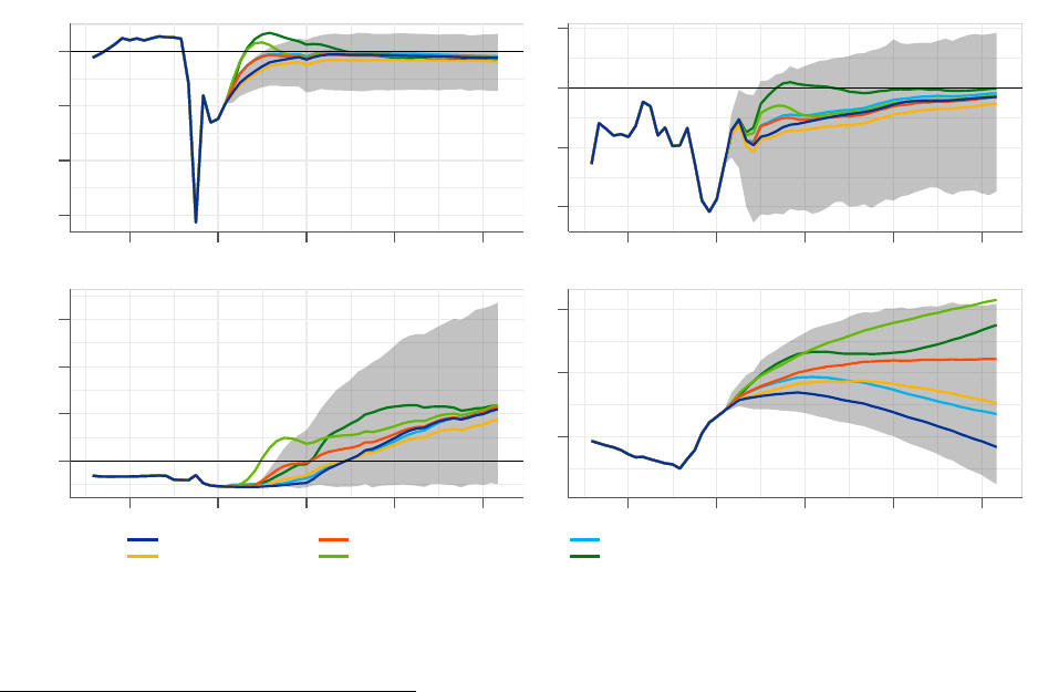
the pessimistic scenario. This implies that stabilisation remains incomplete and inﬂation remains

signiﬁcantly below the target. Only in the most expansionary scenario, inﬂation is temporarily

overshooting, triggering monetary tightening. The positive scenario is characterised by strong do-

mestic demand and signiﬁcant price pressures leading to inﬂation rates approaching 2.5 percent. It

shows that the stabilisation rules switch their sign and bring the output gap to target from above.

Under the positive scenario ﬁscal revenues increase, expenditures are reduced, and nominal output

increases strongly. Consequently, the debt-to-GDP ratio stabilises fast under most combinations of

policy rules.

Figure 14: Post-pandemic stochastic simulations: baseline with variants

-15

-10

-5

2018 2021 2024 2027 2030

Output Gap (% of P

ot. GDP)

2018 2021 2024 2027 2030

Inﬂation (%)

2018 2021 2024 2027 2030

Interest Rate (%)

100

110

2018 2021 2024 2027 2030

Gov. Debt (% of P

ot. GDP)

Baseline

TR & Estimated

TR & Counter-cyclical

TR & Exp.-for-longer II

Low-for-longer II & Counter-cyclical

Low-for-longer III & Exp.-for-longer III

Sources: ECB-BASE simulations.

Notes: The shaded area depicts the 95 percent conﬁdence interval, based on 2000 simulation paths using bootstrapped

residuals centred around the baseline. The lines represent the means.

increases again due to the widening of the distribution. In the tails of the distribution, very negative growth and

inﬂation paths, imply strongly expansionary ﬁscal policy and associated increases in public debt. For the respective

positive realisation, monetary policy is containing the high output realisations via interest rate increases.

ECB Working Paper Series No 2623 / December 2021

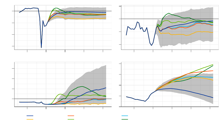
Figure 15: Post-pandemic stochastic simulations: pessimistic growth scenario

-15

-10

-5

2018 2021 2024 2027 2030

Output Gap (% of Pot. GDP)

2018 2021 2024 2027 2030

Inﬂation (%)

2018 2021 2024 2027 2030

Interest Rate (%)

100

110

120

2018 2021 2024 2027 2030

Gov. Debt (% of Pot. GDP)

Baseline

TR & Estimated

TR & Counter-cyclical

TR & Exp.-for-longer II

Low-for-longer II & Coun

ter-cyclical

Low-for-longer III &

Exp.-for-longer III

Sources: ECB-BASE simulations.

Notes: The pessimistic scenario is constructed by choosing the 100 most negative path realisations of output and

depicting the means of these paths and the respective paths of the other variables. See footnote for Figure 14 for

further information.

ECB Working Paper Series No 2623 / December 2021

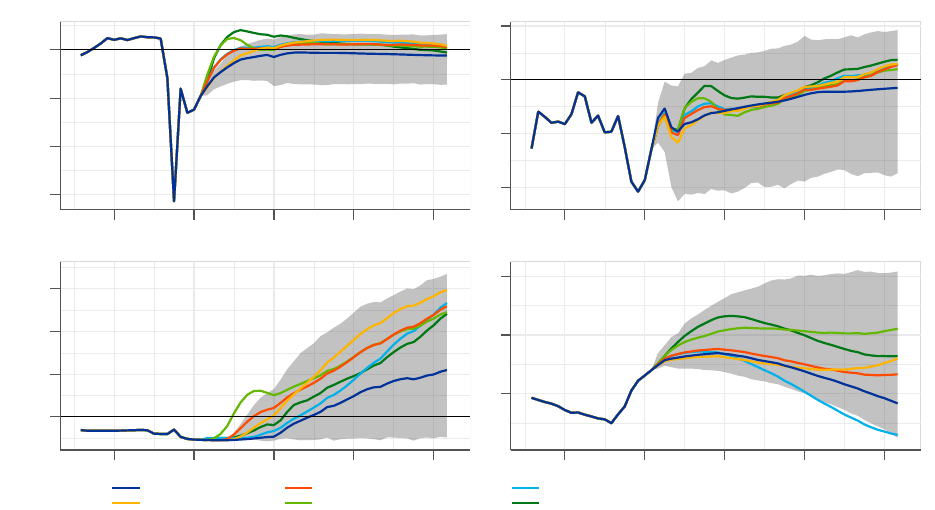
Figure 16: Post-pandemic stochastic simulations: optimistic growth scenario

-15

-10

-5

2018 2021 2024 2027 2030

Output Gap (% of Pot. GDP)

2018 2021 2024 2027 2030

Inﬂation (%)

2018 2021 2024 2027 2030

Interest Rate (%)

100

110

2018 2021 2024 2027 2030

Gov. Debt (% of Pot. GDP)

Baseline

TR & Estimated

TR & Counter-cyclical

TR & Exp.-for-longer II

Low-for-longer II & Coun

ter-cyclical

Low-for-longer III &

Exp.-for-longer III

Sources: ECB-BASE simulations.

Notes: The optimistic scenario is constructed by choosing the 100 most positive path realisations of output and

depicting the means of these paths and the respective paths of the other variables. See footnote for Figure 14 for

further information.

5 Conclusions

Over the foreseeable future ﬁscal policy will have to play a key role in macroeconomic stabilisation

next to monetary policy. This will also apply to the euro area even though its ﬁscal architecture

is incomplete and ﬁscal policies can be expected to largely remain in the hands of national policy-

makers. Still, the existing imperfect set-up should not hinder analysis on desirable economic policies

in the EMU at the aggregate level. In the end, the ﬁscal counterpart to monetary policy is the

aggregate euro area ﬁscal stance.

In this paper we show that a consistently countercyclical ﬁscal policy in the past creates a ﬁscal

buﬀer in the good economic times and it is able to eliminate a large portion of the second downturn

in the euro area. In the future, the combination of the expansionary-for-longer ﬁscal policy and the

ECB Working Paper Series No 2623 / December 2021

low-for-longer monetary policy can be particularly powerful in addressing great challenges faced by

policy-makers, such as large output losses suﬀered by the euro economy amid the pandemic and

inﬂation persistently deviating from the target. Also, our analysis demonstrates that at the current

juncture ﬁscal and monetary policies reinforce each other and mutually create space for each other.

In general, if ﬁscal and monetary policy are coordinated and mutually supportive the real economy

can be stimulated and the inﬂation can be lifted towards its target more eﬀectively and at a lower

cost in terms of the government debt and the ELB duration compared to a situation when the two

policies do not take account of each other.

The results of the macroeconomic simulations are aﬀected by modelling choices and these should

be kept in mind when interpreting the conclusions of the paper. In particular, the ECB-BASE is a

model for the euro area. The aggregation misses important debt sustainability aspects determined

at the country level. Moreover, the simulations are speciﬁc to the considered periods. While a

strong link to the data makes the analysis relevant at the current juncture this comes at the cost of

loosing some generality. Also, in our model an increase in government debt does not lead to negative

repercussions. In reality, however, debt increases are usually costly in terms of future distortionary

taxes or even lead to high rollover risks. In models with rational expectations future consolidations

can limit the immediate impact of expansionary ﬁscal policy. Addressing these simpliﬁcations in the

model could alter the relatively optimistic conclusions of this paper.

ECB Working Paper Series No 2623 / December 2021

References

Angelini, E., N. Bokan, K. Christoﬀel, M. Ciccarelli, and S. Zimic (2019). Introducing ECB-BASE:

The blueprint of the new ECB semi-structural model for the euro area. Working Paper Series 2315,

European Central Bank.

Arias, J., M. Bodenstein, H. T. Chung, T. Drautzburg, and A. Raﬀo (2020). Alternative strategies:

how do they work? how might they help? Finance and Economics Discussion Series 2020-068,

Board of Governors of the Federal Reserve System.

Bassetto, M. and T. J. Sargent (2020). Shotgun wedding: Fiscal and monetary policy. Working

Paper Series 27004, National Bureau of Economic Research.

Benigno, P. and M. Woodford (2003). Optimal monetary and ﬁscal policy: A linear quadratic

approach. Working Paper Series 9905, National Bureau of Economic Research.

Bianchi, F., R. Faccini, and L. Melosi (2020). Monetary and ﬁscal policies in times of large debt:

Unity is strength. Working Paper Series 27112, National Bureau of Economic Research.

Blanchard, O. and R. Perotti (2002). An empirical characterization of the dynamic eﬀects of changes

in government spending and taxes on output. The Quarterly Journal of Economics 117, 1329–

1368.

Brand, C., M. Bielecki, and A. Penalver (2018). The natural rate of interest: estimates, drivers, and

challenges to monetary policy. Occasional Paper Series 27004, European Central Bank.

Cerra, V., A. Fatás, and S. Saxena (2020). Hysteresis and business cycles. IMF Working Paper 20/73,

International Monetary Fund.

Christiano, L., M. Eichenbaum, and S. Rebelo (2011). When is the government spending multiplier

large? Journal of Political Economy 119 (1), 78–121.

Coenen, G., R. Straub, and M. Trabandt (2013). Gauging the eﬀects of ﬁscal stimulus packages in

the euro area. Journal of Economic Dynamics and Control 37 (2), 367–386.

ECB Working Paper Series No 2623 / December 2021

Corsetti, G., L. Dedola, M. Jarociński, B. Maćkowiak, and S. Schmidt (2019). Macroeconomic

stabilization, monetary-ﬁscal interactions, and europe’s monetary union. European Journal of

Political Economy 57, 22–33.

Corsetti, G., K. Kuester, A. Meier, and G. J. Müller (2013). Sovereign risk, ﬁscal policy, and

macroeconomic stability. The Economic Journal 123 (566), F99–F132.

ECB (2016). A guide to the Eurosystem/ECB staﬀ macroeconomic projection exercises. ECB

Article, July 2016 , European Central Bank.

ECB (2020). Eurosystem staﬀ macroeconomic projections for the euro area. ECB Article, December

2020 , European Central Bank.

Eggertsson, G. B. (2011). What ﬁscal policy is eﬀective at zero interest rates? NBER Macroeco-

nomics Annual 25 (1), 59–112.

Eser, F., W. Lemke, K. Nyholm, S. Radde, and A. L. Vladu (2019). Tracing the impact of the ecb’s

asset purchase programme on the yield curve. Working Paper Series 2293, European Central

Bank.

Gali, J. (2015). Monetary Policy, Inﬂation, and the Business Cycle: An Introduction to the New

Keynesian Framework and Its Applications Second edition. Princeton University Press.

Gali, J., J. D. Lopez-Salido, and J. Valles (2007). Understanding the Eﬀects of Government Spending

on Consumption. Journal of the European Economic Association 5 (1), 227–270.

Hauptmeier, S. and C. Kamps (2020). Debt rule design in theory and practice: the SGP’s debt

benchmark revisited. Working Paper Series 2379, European Central Bank.

Hebden, J., E. Herbst, J. Tang, G. Topa, and F. Winkler (2020). How robust are makeup strategies

to key alternative assumptions? Finance and Economics Discussion Series 2020-069, Board of

Governors of the Federal Reserve System.

Holston, K., T. Laubach, and J. C. Williams (2017). Measuring the natural rate of interest: Inter-

national trends and determinants. Journal of International Economics 108, S59–S75.

ECB Working Paper Series No 2623 / December 2021

IMF (2021). After-eﬀects of the covid-19 pandemic: Prospects for medium-term economic damage.

World Economic Outlook, April 2021, Chapter 2 , International Monetary Fund.

Jarociński, M. and M. Lenza (2018). An inﬂation-predicting measure of the output gap in the euro

area. Journal of Money, Credit and Banking 50 (6), 1189–1224.

Kirsanova, T., M. Satchi, D. Vines, and S. Wren-Lewis (2007). Optimal ﬁscal policy rules in a

monetary union. Journal of Money, Credit and Banking 39 (7), 1759–1784.

Leeper, E. M. (1991). Equilibria under âactiveâ and âpassiveâ monetary and ﬁscal policies. Journal

of Monetary Economics 27 (1), 129–147.

Lemke, W. and A. L. Vladu (2017). Below the zero lower bound: a shadow-rate term structure

model for the euro area. Working Paper Series 1991, European Central Bank.

Mendoza, E. G. and V. Z. Yue (2012). A General Equilibrium Model of Sovereign Default and

Business Cycles. The Quarterly Journal of Economics 127 (2), 889–946.

Ramey, V. A. (2019). Ten years after the ﬁnancial crisis: What have we learned from the renaissance

in ﬁscal research? Journal of Economic Perspectives 33 (2), 89–114.

Schmidt, S. (2013). Optimal monetary and ﬁscal policy with a zero bound on nominal interest rates.

Journal of Money, Credit and Banking 45 (7), 1335–1350.

Taylor, J. B. (1999). A Historical Analysis of Monetary Policy Rules. In Monetary Policy Rules,

pp. 319–348. University of Chicago Press.

ECB Working Paper Series No 2623 / December 2021

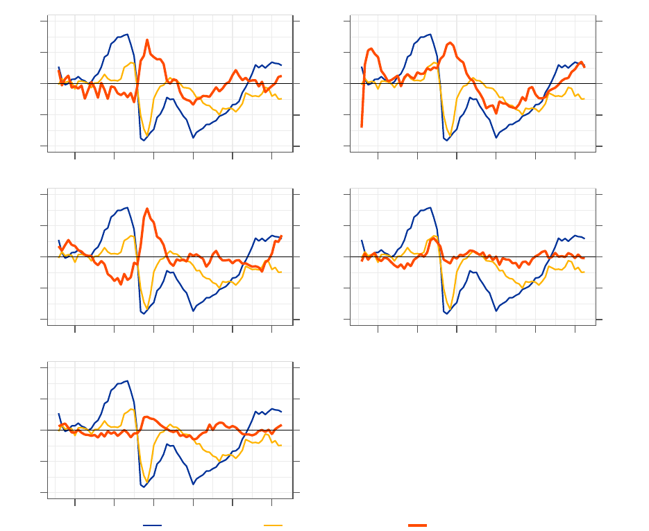
A Government spending instruments over the cycle

Figure A.1: Government spending deviations from a trend (% of potential GDP, unless otherwise

stated)

-4

-2

-0.6

-0.3

0.0

0.3

0.6

2004 2007 2010 2013 2016 2019

Gov. Purchases Gap

-4

-2

-0.6

-0.3

0.0

0.3

0.6

2004 2007 2010 2013 2016 2019

Gov. Investment Gap

-4

-2

-0.6

-0.3

0.0

0.3

0.6

2004 2007 2010 2013 2016 2019

Gov. Transfers Gap

-4

-2

-0.6

-0.3

0.0

0.3

0.6

2004 2007 2010 2013 2016 2019

Gov. Compensation Gap

-4

-2

-0.6

-0.3

0.0

0.3

0.6

2004 2007 2010 2013 2016 2019

Gov. Subsidies Gap

Output Gap (lhs) Inﬂation Gap (pp, lhs) Fiscal Gap (rhs)

Sources: Own calculations based on ECB, Eurostat and European Commission data.

Notes: The chart illustrates deviations from a trend for spending components in the model and contrasts them with

the output gap and inﬂation gap. The size of the deviations is the largest for government purchases, government

investment and government transfers. The movements within the remaining two instruments are considerably more

muted. This observation provides an argument for using the three relatively elastic spending categories as stabilisation

instruments in our exercise.

ECB Working Paper Series No 2623 / December 2021

Table A.1: Coeﬃcients on the output gap in estimated spending rules

Spending category Output gap coeﬃcient

Gov. Purchases -0.01

Gov. Investment 0.00

Gov. Transfers -0.02

Gov. Compensation 0.01

Gov. Subsidies -0.00

Sources: ECB-BASE estimation based on 1999Q1-2019Q4 data.

Notes: The table presents the value of the estimated coeﬃcients on the output gap in estimated ﬁscal rules described

in Subsection 2.1. The values of the coeﬃcients are standardised so that they are comparable to each other even

though the size of spending categories diﬀers signiﬁcantly. The estimated ﬁgures are consistent with the illustration

in Figure A.1. Most notably, they are the most negative for categories that move in the opposite direction to the

output gap (see gov. transfers). Nevertheless, they are small compared to -0.1 value assumed in our countercyclical

rule.

B Detailed presentation of ﬁscal and monetary policy rules

Fiscal Policy rules

• Estimated ﬁscal rule

∆g

= α(g

t−1

− g

t−1

) + δ∆g

k=1

∆g

t−k

+ γ

(

−

b) + ε

(B.1)

Where g

is log of actual spending (i.e. investments, purchases or transfers), g

is log of trend

spending,

is the real output gap,

is the debt ratio to nominal output,

b is the debt target

and ε

the residual term.

Coeﬃcients are estimated over 1999Q1-2019Q4 and the one associated with the output gap turns

out to be close to 0 (i.e. γ

≈ 0).

• Countercyclical ﬁscal rule

∆g

= α(g

t−1

− g

t−1

) + δ∆g

k=1

∆g

t−k

+ γ

(

−

b) + ε

(B.2)

Where γ

 0, which makes this rule diﬀerent (i.e. countercyclical) compared to the estimated

one.

ECB Working Paper Series No 2623 / December 2021

• Expansionary-for-longer ﬁscal rules

With i ∈ {nom, real},

∆g

= α(g

t−1

− g

t−1

) + δ∆g

k=1

∆g

t−k

+ γ

aug,i

+ γ

(

−

b) + ε

(B.3)

Where γ

 0 and

aug,i

is the augmented output gap deﬁned with the nominal or real approach.

∗ Nominal approach (i = nom)

aug,nom

+ 1 [R

≤ 0]

(B.4)

Where R

is the nominal short-term rate, and

is the price gap calculated as a discounted

cumulation of inﬂation gaps (ˆπ

)

∞

k=0

ˆπ

t−k

(B.5)

The higher the β coeﬃcient the longer the memory of the cumulation process.

Exp.-for-longer I Exp.-for-longer II Exp.-for-longer III

β 0.9 0.925 0.95

∗ Real approach (i = real)

aug,real

+ 1 [R

≤ 0]

add

(B.6)

Where R

is the nominal short-term rate, and

add

is the cumulative output shortfalls deﬁned

add

= ρ

add

t−1

k=1

t−k+1

≤ 0

t−k+1

(B.7)

ECB Working Paper Series No 2623 / December 2021

add

and a

coeﬃcients are calibrated so that the real approach results in broadly the same like

the one calculated with the nominal approach. The importance of the past output shortfalls in the

formula (as judged by

k=1

) increases with the degree to which ﬁscal policy remains expansionary-

for-longer.

Exp.-for-longer I Exp.-for-longer II Exp.-for-longer III

k=1

0.056 0.064 0.070

Monetary Policy rules

• Standard Taylor rule

= max

0.85R

t−1

+ 0.15(r

∗

+ ¯π

+ ( ¯π

− π

∗

)), −0.5

+ ε

(B.8)

Where r

∗

is the natural interest rate, ¯π

the inﬂation,

is the real output gap, π

∗

the inﬂation

target and ε

the residual term.

• Low-for-longer monetary rules

Expansionary-for-longer monetary rules used in this paper correspond to average inﬂation targeting

rules and can be deﬁned as follows

= max

0.85R

t−1

+ 0.15(r

∗

+ ¯π

+ T ( ¯π

(T −year )

− π

∗

)), −0.5

+ ε

(B.9)

Where ¯π

(T −year )

is the average inﬂation over (T − year) period.

Low-for-longer I Low-for-longer II Low-for-longer III

(T − year) 2 3 4

ECB Working Paper Series No 2623 / December 2021

Acknowledgements

We would like to thank Ettore Dorrucci, Marien Ferdinandusse, Sebastian Hauptmeier, Nadine Leiner-Killinger, Klaus Masuch, Leopold

von Thadden and Isabel Vansteenkiste for valuable comments.

The views expressed in this paper, as well as all errors and omissions, should be regarded as those of the authors and are not

necessarily those of the European Central Bank.

Krzysztof Bańkowski

European Central Bank, Frankfurt am Main, Germany; email: krzysztof.bank[email protected]

Kai Christoffel

European Central Bank, Frankfurt am Main, Germany; email: [email protected]

Thomas Faria

European Central Bank, Frankfurt am Main, Germany; email: [email protected].eu

Postal address 60640 Frankfurt am Main, Germany

Telephone +49 69 1344 0

Website www.ecb.europa.eu

electronically, in whole or in part, is permitted only with the explicit written authorisation of the ECB or the authors.

This paper can be downloaded without charge from www.ecb.europa.eu, from the Social Science Research Network electronic library or

from RePEc: Research Papers in Economics. Information on all of the papers published in the ECB Working Paper Series can be found

on the ECB’s website.

PDF ISBN 978-92-899-4910-1 ISSN 1725-2806 doi:10.2866/292369 QB-AR-21-114-EN-N