
Finance and Economics Discussion Series
Divisions of Research & Statistics and Monetary Affairs
Federal Reserve Board, Washington, D.C.
Redistribution and the Monetary–Fiscal Policy Mix
Saroj Bhattarai, Jae Won Lee, Choongryul Yang
2021-013
Please cite this paper as:
Bhattarai, Saroj, Jae Won Lee, and Choongryul Yang (2021). “Redistribu-
tion and the Monetary–Fiscal Policy Mix,” Finance and Economics Discussion Se-
ries 2021-013. Washington: Board of Governors of the Federal Reserve System,
https://doi.org/10.17016/FEDS.2021.013.
NOTE: Staff working papers in the Finance and Economics Discussion Series (FEDS) are preliminary
materials circulated to stimulate discussion and critical comment. The analysis and conclusions set forth
are those of the authors and do not indicate concurrence by other members of the research staff or the
Board of Governors. References in publications to the Finance and Economics Discussion Series (other than
acknowledgement) should be cleared with the author(s) to protect the tentative character of these papers.

Redistribution and the Monetary–Fiscal Policy Mix
∗
Saroj Bhattarai
†
Univ. of Texas-Austin
and CAMA
Jae Won Lee
‡
Univ. of Virginia
Choongryul Yang
§
Federal Reserve Board
Abstract
We show that the effectiveness of redistribution policy in stimulating the economy
and improving welfare is directly tied to how much inflation it generates, which in
turn hinges on monetary-fiscal adjustments that ultimately finance the transfers. We
compare two distinct types of monetary-fiscal adjustments: In the monetary regime, the
government eventually raises taxes to finance transfers, while in the fiscal regime, in-
flation rises, effectively imposing inflation taxes on public debt holders. We show ana-
lytically in a simple model how the fiscal regime generates larger and more persistent
inflation than the monetary regime. In a quantitative application, we use a two-sector,
two-agent New Keynesian model, situate the model economy in a COVID-19 reces-
sion, and quantify the effects of the transfer components of the Coronavirus Aid, Re-
lief, and Economic Security (CARES) Act. We find that the transfer multipliers are sig-
nificantly larger under the fiscal regime—which results in a milder contraction—than
under the monetary regime, primarily because inflationary pressures of this regime
counteract the deflationary forces during the recession. Moreover, redistribution pro-
duces a Pareto improvement under the fiscal regime.
JEL classification: E53; E62; E63
Keywords: Household heterogeneity, Redistribution, Monetary-fiscal policy mix, Trans-
fer multiplier, Welfare evaluation, COVID-19, CARES Act
∗
We thank Woong Yong Park for helpful comments. The views expressed here are those of the authors
and do not necessarily reflect those of the Federal Reserve Board or the Federal Reserve System. First
version: Dec 2020. This version: Jan 2021.
†
Department of Economics, University of Texas at Austin and CAMA, 2225 Speedway, Stop C3100,
Austin, TX 78712, U.S.A. Email: [email protected].
‡
Department of Economics, University of Virginia, PO BOX 400182, Charlottesville, VA 22904, U.S.A.
Email: [email protected].
§
Federal Reserve Board of Governors, 20th Street and Constitution Avenue NW, Washington, DC 20551,
U.S.A. Email: [email protected].
1

1 Introduction
What are the macroeconomic effects of redistribution policies that transfer resources from
one set of agents in the economy to another? What are the determinants of the transfer
multiplier? When is the transfer multiplier large? What are the welfare implications of
such redistribution policies?
Recently, the U.S. experienced the two largest contractions after World War II—the
Great Recession and the COVID-19 recession. The government responded to these con-
tractions with unprecedented fiscal measures—namely the American Recovery and Rein-
vestment Act of 2009 and the Coronavirus Aid, Relief, and Economic Security (CARES)
Act of 2020. These fiscal responses included significant transfer components, and they
have renewed interest in the effectiveness of transfer policies in terms of rebooting the
economy and improving household welfare.
In a dynamic general equilibrium model, one would have to take numerous factors
into account to answer the above questions.
1
In this paper, we focus on the source of
financing and show how the government finances transfers has a first-order importance
for their effectiveness. Our focus is motivated by the ongoing rapid increase in public
debt caused by the large-scale transfer programs. This eventually requires fiscal and/or
monetary adjustments, which would ultimately finance current transfers.
We compare two distinct ways to finance transfers in a two-agent New Keynesian
(TANK) model. In the model, a set of households are unable to borrow and lend to smooth
consumption over time. A transfer policy redistributes resources toward such "hand-to-
mouth" (HTM) households and away from "Ricardian" households that own government
bonds.
2
In the first policy regime, the government raises taxes. Inflation is then stabilized
in the usual way by the central bank. We call this case the "monetary regime." In the
second regime, the government commits itself to no adjustments in taxes, and the central
bank allows inflation to rise to stabilize the real value of debt, thereby imposing "inflation
taxes" on households that hold nominal government debt. In this "fiscal regime," the fiscal
theory of the price level operates.
We find that the effectiveness of transfer policy is directly tied to how much inflation
it generates. A transfer policy is inflationary irrespective of the policy regimes in the
model. It is, however, more inflationary in the fiscal regime than in the monetary regime.
1
We discuss previous findings in more detail later. Some well-known determinants of the fiscal mul-
tiplier are the marginal propensity to consume of targeted households and whether the economy is in a
liquidity trap.
2
As we describe in further detail later, in our application, we think of these HTM households as working
in the service sector that is affected by a large negative sectoral shock.
2

Therefore, inflation-financed transfers can be used to fight deflationary pressures during
recessions, thereby preventing output and consumption of both types of households from
dropping significantly. As a result, the welfare of both household types is higher when
transfers are inflation-financed than when they are tax-financed.
Furthermore, somewhat surprisingly, inflation-financed transfers can produce a Pareto
improvement relative to the no-transfer case. Notice that, since the model features stag-
gered Calvo-type price setting, inflation is not a free lunch: it generates, ceteris paribus,
significant resource misallocation, which leads to a decrease in labor productivity and
in welfare. These negative effects of inflation are, however, outweighed by the positive
effects of inflation in the low-inflation environment considered in this paper. In fact, with-
out an inflationary intervention, the economy would experience deflation, so there is little
cost of inflation.
Our paper starts with a simplified flexible-price version of the model that permits
analytical results, thereby allowing us to illuminate the mechanism of the fiscal theory
in a heterogeneous-household framework. This model also serves as a useful reference
point, as the two policy regimes produce exactly the same multipliers for output and
consumption and an identical level of household welfare, even if inflation dynamics are
different. This is due to two features. First, both conventional taxes, which are assumed
to be lump sum, and inflation taxes are non-distortionary. Second, price flexibility shuts
down any feedback effects from inflation on real variables.
3
For inflation, the fiscal regime gives rise to higher and more persistent inflation than
the monetary regime. In particular, transfers affect inflation through two channels in
this regime. First, an increase in transfers leads directly to an increase in public debt,
which accumulates over time. Consequently, inflation rises to stabilize the real value of
debt. Second, an increase in transfers may indirectly raise future public debt through an
interest rate channel. Redistribution changes Ricardian household consumption, which in
turn affects real interest rates and thus outstanding public debt in the following periods.
That is, redistribution generates a new valuation effect through real interest rate changes,
an effect that is absent in the standard one-agent model often used to analyze the fiscal
regime. This interest rate channel may lead to a further increase in inflation. Showing
these two effects explicitly in a nonlinear two-agent model is a contribution of our paper.
We then build on the analytical results and proceed to a quantitative analysis employ-
ing a two-sector TANK model. Relative to the simplified version, the quantitative model
3
The transfer multiplier for output is small yet still positive due to the classical labor supply channel.
Redistribution causes Ricardian household consumption to fall, creating a negative “wealth effect” on labor
supply. The households thus supply more hours for a given wage rate, which in turn raises output.
3

includes several realistic features that break the uniformity of the two regimes in terms of
the multipliers. The two most important are nominal rigidities and the "COVID shocks."
Sticky prices are important, as transfers now can increase output through the usual New
Keynesian channel by generating inflation—on top of the classical labor supply channel.
Introducing shocks is also consequential as the multipliers are generally state-dependent.
In particular, the COVID shocks cause the economy to fall into what we refer to as a
"COVID recession" as well as a liquidity trap, in which the effects of redistribution can be
different quantitatively. Finally, another difference from the analytical model is that the
government raises (gradually) labor taxes, rather than lump-sum taxes, in the monetary
regime, which, through distortionary effects, influences the transfer multipliers.
Specifically, in order to capture the salient characteristics of the COVID recession, we
suppose that the COVID shocks consist of adverse aggregate and sector-specific demand
shocks and sector-specific labor supply shocks. The sector-specific shocks intend to cap-
ture the observation that "locked out" of work and fear of "unsafe consumption" features
are more pronounced in certain sectors of the economy. We decompose the U.S. economy
into two sectors—(1) transportation, recreation, and food service sector and (2) the rest of
the economy—and let the HTM households work in the former sector in our model.
4
For
convenience, we call this sector the HTM sector.
Figure 1 presents dynamics of employment, hours, inflation, and consumption based
on such a two-sector decomposition of the U.S. economy. As is clear, there was a sharp ad-
verse effect on employment/hours in the HTM sector following the COVID crisis. More-
over, inflation in this sector also fell. Finally, while the HTM sector was disproportionately
affected, there was also an aggregate, economy-wide contraction and fall in inflation as
well. We calibrate the COVID shocks to perfectly re-produce the dynamics of hours in
the two sectors and that of inflation in the HTM sector, thereby situating the model econ-
omy in a COVID-recession-like environment. We then calibrate the size of transfers to
match the transfer amount in the CARES Act and study how the economy responds to
the redistribution policy under several alternative scenarios.
5
We find that the transfer multipliers are significantly larger under the fiscal regime
than under the monetary regime, primarily because of the difference in inflation dynam-
ics as mentioned above. For instance, the four-year cumulative multiplier for aggregate
output is 1.126 in the monetary regime while it is 7.739 in the fiscal regime. Notice that
this multiplier is greater than unity even under the monetary regime, thanks to nom-
4
We assume that the Ricardian households work in the other sectors that are less affected by the COVID
pandemic.
5
We also show with the vertical dashed line in Figure 1 when transfer payments from the CARES Act
started to get mailed.
4
−−> CARES Act (Apr. 15)
−40
−30
−20
−10
0
Percent Deviation from Jan. 2020
1 2 3 4 5 6 7 8
2020
Total
Retail, Transportation,
Leisure and Hospitality
Others
Panel A: Employment
−40
−30
−20
−10
0
Percent Deviation from Jan. 2020
1 2 3 4 5 6 7 8
2020
Total
Retail, Transportation,
Leisure and Hospitality
Others
Panel B: Total Hours
−70
−60
−50
−40
−30
−20
−10
0
10
Percent Deviation from Jan. 2020
1 2 3 4 5 6 7 8
2020
Total
Transportation, Recreation,
and Food Services
Others
Panel C: Real PCE
−2
−1.5
−1
−.5
0
.5
1
Percent Deviation from Jan. 2020
1 2 3 4 5 6 7 8
2020
Total
Transportation, Recreation,
and Food Services
Others
Panel D: PCE Inflation
Figure 1: Aggregate and Sectoral Effects of COVID Crisis
Notes: This figure shows the dynamics of key variables from January 2020. Panels A and B show employ-
ment and total hours dynamics in U.S. Bureau of Labor Statistics, respectively. Black lines are dynamics
of total variable and red lines represent retail, transportation, leisure, and hospitality sector, and blue
lines represent all other sectors. Panels C and D present real personal consumption expenditure and
PCE inflation in U.S. Bureau of Economic Analysis, respectively. Black lines are dynamics of total vari-
able and red lines represent transportation, recreation and food services sector, and blue lines represent
all other sectors.
Sources: U.S. Bureau of Economic Analysis, U.S. Bureau of Labor Statistics
inal rigidities and the binding zero lower bound (ZLB). Just as strikingly different are
the four-year cumulative consumption multipliers. For the Ricardian households, it is
negative 0.244 in the monetary regime and 6.036 in the fiscal regime, while for the HTM
households, it is 5.609 in the monetary regime and 13.311 in the fiscal regime.
6
We isolate the role played by various model elements in driving our quantitative re-
6
The positive consumption multiplier for the Ricardian household is unique, even qualitatively so, in
the fiscal regime.
5

sults using counterfactual exercises. The unusually large multipliers reported above, es-
pecially under the fiscal regime, result from the economy being situated in the historically
severe COVID-recession with large deflationary pressures. For example, shutting down
the COVID shocks, the four-year cumulative multiplier for aggregate output is 0.96 in the
monetary regime, while it is 1.475 in the fiscal regime. This result underscores the state-
dependency of policy effects. Importantly, the difference in the multipliers for output
and consumption between the two regimes gets larger in the presence of COVID shocks,
which implies that while both labor-tax-financed transfers and inflation-financed trans-
fers are more effective in the COVID recession than in a normal environment, the latter is
even more so. In addition, we also find that relying on labor taxes rather than lump-sum
taxes in the monetary regime plays a role.
Overall, as a consequence, the contraction in output and consumption is much more
muted when transfers are financed by inflation taxes. Specifically, transfers, when inflation-
financed, would reduce the output loss caused by the COVID shocks by roughly 5 per-
centage points at the trough compared to no-intervention case. We also find that the
expansionary effects of inflation-financed transfers are so large that such redistribution
policy generates a Pareto improvement: It increases the welfare of both the recipients and
sources of transfers, even taking into account the resources taken away from the Ricar-
dian household and the fact that the Ricardian household’s leisure decreases as a result
of output increases and distortions generated by high and persistent inflation.
Our paper builds on several strands of the literature. It is related to the fiscal-monetary
interactions literature as originally developed in Leeper (1991), Sims (1994), Woodford
(1994), Cochrane (2001), Schmitt-Grohé and Uribe (2000), and Bassetto (2002).
7
Sims
(2011) introduced long-term debt under this regime in a sticky price model, while Cochrane
(2018) developed it further to analyze the inflation implications following the Great Re-
cession. Analytical characterization of the fiscal regime in a linearized sticky price model
is in Bhattarai, Lee and Park (2014).
Our additional analytical contribution here is to derive the fully nonlinear results of
this fiscal regime in a tractable two-agent model. Motivated by the COVID crisis and the
CARES Act, we then assess the quantitative effects of redistribution policy as well as its
welfare implications in a two-sector, two-agent nonlinear model.
We build on two-agent models as originally developed in Campbell and Mankiw
(1989), Galí, López-Salido and Vallés (2007), and Bilbiie (2018). Moreover, Bilbiie, Mona-
celli and Perotti (2013), closely related to this paper, show that different financing schemes
affect the size of the output transfer multiplier in a TANK model. However, they only
7
Canzoneri, Cumby and Diba (2010) and Leeper and Leith (2016) are recent surveys of this literature.
6

consider the monetary regime. Our main contribution is in assessing the effects of redis-
tribution policy in such an environment and showing how it depends critically on the
monetary-fiscal policy mix.
Recently there have been several contributions to an analysis of macroeconomic ef-
fects of the COVID crisis. Our quantitative two-sector, two-agent model is closest to the
important work of Guerrieri, Lorenzoni, Straub and Werning (2020). In assessing the
quantitative effects of fiscal policy during the pandemic using a model with household
heterogeneity, we are also related to Faria-e-Castro (2020) and Bayer, Born, Luetticke and
Müller (2020). Our relative contribution is in showing how the effects of redistribution
depend on the monetary-fiscal policy regime and then assessing both quantitative effects
and welfare implications by matching some important aggregate and sectoral aspects of
the U.S. data.
Our paper is also related to recent papers that analyze monetary-fiscal policy interac-
tions in TANK models—in particular, Bhattarai, Lee, Park and Yang (2020), Bianchi, Fac-
cini and Melosi (2020), and Motyovszki (2020). Bhattarai, Lee, Park and Yang (2020) study
the effects of one-time permanent capital tax rate changes in a model that also features
capital-skill complementarity. Bianchi, Faccini and Melosi (2020) and Motyovszki (2020)
are motivated by the COVID crisis and are closely related to our analysis.
8
Our relative
contribution analytically is a nonlinear solution of the simple TANK model under the two
regimes. On the quantitative side, while these studies focus on the positive implications
of transfers under the different regimes, we additionally provide welfare implications for
different types of households. We also emphasize that the positive and normative im-
plications of redistribution are state-dependent and that inflation-financed transfers are
disproportionately more effective than tax-financed transfers in a COVID-recession-like en-
vironment in which both sector-specific and aggregate shocks hit the economy.
Finally, our paper is also related to the government spending multiplier literature, as
the effects of transfer policy in two-agent models share some common elements with the
effects of government spending policy in representative agent models. Thus, in connect-
ing the effects to the nature of monetary policy, the binding ZLB, and the monetary-fiscal
policy regime, our work builds on important contributions in the government spend-
ing multiplier literature by Woodford (2011), Christiano, Eichenbaum and Rebelo (2011),
Eggertsson (2011), Leeper, Traum and Walker (2017), and Jacobson, Leeper and Preston
(2019).
8
Bianchi, Faccini and Melosi (2020) show that inflating away a targeted fraction of debt will increase
the effectiveness of the fiscal stimulus in a rich medium-scale model while Motyovszki (2020) considers a
small-open economy environment.
7

2 Simple Model and Redistribution Policy
We present a simple model that yields analytical results on effects of redistribution policy.
2.1 Model
There are two types of households: Ricardian and HTM. The Ricardian household makes
optimal labor supply and consumption/savings decisions, while the HTM household
simply consumes government transfers every period. In this setup, we analytically show
the effects on inflation of transferring resources away from the Ricardian households to
the HTM households and point out that these effects depend critically on how the transfer
policy is financed.
2.1.1 Households
Ricardian Households. There are Ricardian households of measure 1 − λ. These house-
holds, taking prices as given, choose {C
R
t
, L
R
t
, B
R
t
} to maximize
∞
∑
t=0
β
t
"
log C
R
t
− χ
L
R
t
1+ϕ
1 + ϕ
#
subject to a standard No-ponzi-game constraint and a sequence of flow budget constraints
C
R
t
+
B
R
t
P
t
= R
t−1
B
R
t−1
P
t
+ w
t
L
R
t
+ Ψ
R
t
− τ
R
t
,
where C
R
t
is consumption, L
R
t
is hours, B
R
t
is nominal government debt, Ψ
R
t
is real profits,
τ
R
t
is lump-sum taxes, P
t
is the price level, w
t
is the real wage, and R
t
is the nominal gross
interest rate. The discount factor and the inverse of the Frisch elasticity are denoted by
β ∈ ( 0, 1) and ϕ ≥ 0 respectively. The superscript, R, represents “Ricardian”. The flow
budget constraints can be written as
C
R
t
+ b
R
t
= R
t−1
1
Π
t
b
R
t−1
+ w
t
L
R
t
+ Ψ
R
t
− τ
R
t
,
where b
R
t
=
B
R
t
P
t
is the real value of debt, and Π
t
=
P
t
P
t−1
is the gross rate of inflation.
Optimality conditions are given by the Euler equation, the intra-termporal labor sup-
ply condition, and the transversality condition (TVC):
C
R
t+1
C
R
t
= β
R
t
Π
t+1
, (2.1)
8

χ
L
R
t
ϕ
C
R
t
= w
t
, (2.2)
lim
t→∞
β
t
1
C
R
t
B
R
t
P
t
= 0. (2.3)
Hand-to-Mouth Households. The hand-to-mouth (HTM) households, of measure λ,
simply consume government transfers, s
H
t
, every period
C
H
t
= s
H
t
,
and have no optimization problem to solve. The superscript, H, represents “HTM”.
2.1.2 Firm
A representative firm in the competitive product market chooses hours, L
t
, in each period
to maximize profits:
Ψ
t
= Y
t
− w
t
L
t
,
subject to the production function
Y
t
= L
t
. (2.4)
Zero profit condition implies
w
t
= 1. (2.5)
2.1.3 Government
The government issues one-period nominal debt, B
t
. Its budget constraint (GBC) is
B
t
P
t
= R
t−1
B
t−1
P
t
− τ
t
+ s
t
,
where s
t
is transfers and τ
t
is taxes. It can be re-written as
b
t
=
R
t−1
Π
t
b
t−1
− τ
t
+ s
t
, (2.6)
where b
t
=
B
t
P
t
is the real value of debt. Transfer, s
t
, is exogenous and deterministic.
Monetary and tax policy rules are
R
t
¯
R
=
Π
t
¯
Π
φ
, (2.7)
(
τ
t
−
¯
τ
)
= ψ(b
t−1
−
¯
b), (2.8)
9

where φ and ψ determine the responsiveness of the policy instruments to inflation and
government indebtedness respectively. The steady-state values of inflation, debt, and
transfers,
¯
Π,
¯
b,
¯
s
, are set by policymakers and given exogenously.
2.1.4 Aggregation and the Resource Constraint
Aggregating the variables over the households yields s
t
= λs
H
t
, τ
t
=
(
1 − λ
)
τ
R
t
, b
t
=
(
1 − λ
)
b
R
t
, L
t
=
(
1 − λ
)
L
R
t
, and Ψ
t
=
(
1 − λ
)
Ψ
R
t
. Combining household and govern-
ment budget constraints gives:
(1 − λ)C
R
t
+ λC
H
t
= Y
t
.
The resource constraint above, together with the HTM household budget constraint, im-
plies that output is simply divided between the two types of households as:
C
H
t
=
1
λ
s
t
, C
R
t
=
1
1 − λ
Y
t
−
1
1 − λ
s
t
. (2.9)
2.2 Effects of Redistribution Policy
We now show the effects of transferring resources away from the Ricardian households
to the HTM households. The government can finance such a transfer program in two
distinct ways. In the first policy regime, the government raises taxes sufficiently. Inflation
is then stabilized in the usual way by the central bank. In the second regime, the govern-
ment does not raise taxes, and the central bank allows inflation to rise to stabilize the real
value of debt, thereby imposing “inflation taxes” on the Ricardian households that hold
nominal government debt. The fiscal theory of the price level operates in this case.
We solve for the equilibrium time path of
Y
t
, C
R
t
, C
H
t
, Π
t
, R
t
, b
t
, τ
t
given exogenous
{
s
t
}
. Output and consumption of the two households, and thus their welfare, are in-
dependent of whether the government relies on conventional or inflation taxes.
9
We
first consider those policy-invariant variables in Section 2.2.1. The alternative financing
schemes, however, generate quite different inflation dynamics, which is the main focus
of this simple model. The rise of inflation tends to be greater and more persistent in the
second regime. The determination of the rate of inflation is detailed in Section 2.2.2.
9
This “neutrality” result does not hold in a model with nominal rigidities, as discussed in detail later.
10

2.2.1 Output and Consumption
We start with output. Equation (2.2) can be written as
Y
t
= χ
−1
(
1 − λ
)
1+ϕ
Y
−ϕ
t
+ s
t
(2.10)
using Equations (2.4), (2.5), and (2.9). Equation (2.10) implicitly defines output as a func-
tion of transfers: Y
t
= Y
(
s
t
)
. Then, one can obtain the “transfer multiplier” as
dY
(
s
t
)
ds
t
=
1
1 +
(
1 − λ
)
1+ϕ
ϕ
χ
Y
−
(
1+ϕ
)
t
.
Notice that 0 ≤
dY
t
ds
t
≤ 1.
An increase in transfers raises output not for the Keynesian demand-side reason. The
channel here instead is purely classical and supply-side: An increase in s
t
causes Ricar-
dian household consumption to fall, creating a negative “wealth effect” on labor supply.
The households supply more hours for a given wage rate, which in turn raises output.
10
The multiplier is maximized (dY
t
/ds
t
= 1) when labor supply is perfectly elastic (ϕ = 0)
while it is minimized (dY
t
/ds
t
= 0) when the Ricardian household does not value leisure
(χ = 0), which shuts down the wealth effect.
The Ricardian household consumption is obtained from Equation (2.9) as
C
R
t
= C
R
(
s
t
)
≡
1
1 − λ
[
Y
(
s
t
)
− s
t
]
. (2.11)
The derivative is
dC
R
(
s
t
)
ds
t
=
1
1 − λ
dY
(
s
t
)
ds
t
− 1
≤ 0.
As will be clear below, how Ricardian household consumption depends on transfers mat-
ter for inflation dynamics as it affects the real interest rate. That is, there is a valuation
effect on government debt due to changes in the real interest rate. This interest rate channel
of transfers is absent in the model with a representative household, where transfers have
no redistributive role, or with a perfectly elastic labor supply.
Notice that both tax types are non-distorting in this model. Consequently, for given
{
s
t
}
, the alternative ways to finance transfers (i.e., the policy regimes) have no effect on
output and consumption, as seen above.
10
The channel thus is the same as the effect of government spending in a one-agent model.
11

2.2.2 Inflation
We now turn to the rest of the variables,
{
Π
t
, R
t
, b
t
, τ
t
}
∞
t=0
, with a focus on inflation de-
termination, given a path of
{
s
t
}
∞
t=0
. The equilibrium time path of
{
Π
t
, R
t
, b
t
, τ
t
}
satisfies
the following conditions:
• Difference Equations from (2.1), (2.6), (2.7) and (2.8):
Π
t+1
=
C
R
t
C
R
t+1
βR
t
, b
t
= R
t−1
b
t−1
1
Π
t
− τ
t
+ s
t
,
R
t
¯
R
=
Π
t
¯
Π
φ
,
(
τ
t
−
¯
τ
)
= ψ(b
t−1
−
¯
b).
• Terminal condition, as given by TVC from Equation (2.3):
lim
t→∞
β
t
1
C
R
t
b
t
= 0.
• Initial conditions:
b
−1
and R
−1
.
We first solve for the deterministic steady state. When s
t
=
¯
s ∀t, the system of differ-
ence equations simplifies to
¯
R = β
−1
¯
Π,
¯
τ =
β
−1
− 1
¯
b +
¯
s,
with the TVC trivially satisfied. Given
¯
s,
¯
Π and
¯
b, which we assume exogenously deter-
mined by policymakers, the equations above determine
¯
R and
¯
τ. We set R
−1
=
¯
R and
b
−1
=
¯
b, without loss of generality.
The system of difference equations can be simplified as
11
:
Π
t+1
¯
Π
=
C
R
t
C
R
t+1
Π
t
¯
Π
φ
, (2.12)
b
t
−
¯
b
=
"
β
−1
C
R
t
C
R
t−1
− ψ
#
(b
t−1
−
¯
b) +
(
s
t
−
¯
s
)
+
¯
b
"
β
−1
C
R
t
C
R
t−1
− β
−1
#
∀t ≥ 1 (2.13)
b
0
−
¯
b
= β
−1
¯
Π
Π
0
− 1
¯
b +
(
s
0
−
¯
s
)
at t = 0, (2.14)
which determines
{
Π
t
, b
t
}
given
{
s
t
}
and
C
R
t
, where note that from Equation (2.11),
the latter is a simple function of transfers.
11
The online appendix provides detail.
12

Equation (2.12), obtained by combining the Euler equation and the monetary policy
rule, shows how future inflation (Π
t+1
) depends on current inflation (Π
t
) and the real
rate captured by C
R
t+1
/C
R
t
. Equation (2.13) is the GBC for t ≥ 1 after we substitute out the
nominal interest rate (R
t−1
) and taxes (τ
t
) using the Euler equation and the fiscal policy
rule. Equation (2.14) is the GBC at t = 0. This looks different from Equation (2.13) because
R
−1
is exogenous, and thus cannot be replaced by the Euler equation.
Equation (2.13) describes how the deviation of the real value of debt from the steady
state,
b
t
−
¯
b
, evolves over time. An increase in transfers over its steady state value
(s >
¯
s) affect debt dynamics directly and indirectly. First, ceteris paribus, such an increase
causes b
t
, debt carried over to the next period, to rise above
¯
b. This direct effect is captured
by the second term,
(
s
t
−
¯
s
)
, on the right hand side of Equation (2.13). Second, a change
in transfers affects Ricardian household consumption as shown in Equation (2.11) and
hence the real interest rate, which in turn influences debt dynamics. This indirect effect is
reflected by r
t−1
≡ β
−1
C
R
t
C
R
t−1
in Equation (2.13), and operates even when the current period
debt stays at the steady state (i.e. b
t−1
=
¯
b). The reason is a change in interest payments
for a given amount of debt—as shown in the last term,
¯
b
β
−1
C
R
t
C
R
t−1
− β
−1
.
In solving the system, we consider a redistribution program in which
{
s
t
}
∞
t=0
can have
arbitrary values greater than
¯
s until a time period T, and then s
t
=
¯
s for t ≥ T + 1. In this
case, regardless of the history until time T + 1, starting T + 2, Equation (2.13) becomes
b
t
−
¯
b
=
β
−1
− ψ
(b
t−1
−
¯
b).
How the TVC is satisfied depends on the fiscal policy parameter ψ. When ψ > 0, debt
dynamics satisfies the TVC regardless of the value of b
T+1
.
12
When ψ ≤ 0, however, the
TVC requires b
T+1
=
¯
b, which can be achieved when monetary policy allows inflation to
adjust by the required amount. Below, we discuss each case in turn.
Inflation under the Monetary Regime. When ψ > 0, , inflation is solely determined by
Equation (2.12) which becomes
Π
t+1
¯
Π
=
Π
t
¯
Π
φ
for t ≥ T + 1,
as C
R
t
, Ricardian household consumption, is constant. In this case, if we were to consider
φ < 1, the system of Equations (2.12)–(2.14) does not pin down initial inflation Π
0
, and
the model permits multiple non-explosive solutions.
12
In addition, ψ should not be too big. We do not explicitly consider such empirically irrelevant cases.
13

We therefore, instead consider the standard case, φ > 1, which we call the monetary
regime. This regime produces multiple equilibria in which inflation is unbounded and a
unique bounded equilibrium.
13
Here we focus on the bounded equilibrium. In this case,
it is necessary that
Π
T+1
¯
Π
= 1.
Given this “stability” condition on inflation, one can pin down Π
t
from t = 0 to T along
the saddle path. In particular, inflation before T + 1 can be solved backward using Equa-
tion (2.12). The initial inflation is given by
Π
0
¯
Π
= C
R
(
¯
s
)
1
φ
T+1
1
C
R
(
s
T
)
C
R
(
s
T−1
)
· · · C
R
(
s
0
)
1
φ
=
T
∏
t=0
C
R
(
¯
s
)
C
R
(
s
t
)
1
φ
. (2.15)
Inflation in the following periods is then determined by Equation (2.12).
Equation (2.15) shows that an increase in transfers is inflationary as the Ricardian
household consumption declines below the pre-transfer level. The magnitude of the ef-
fect depends on the response of monetary policy (measured by φ), the size of transfer
increases, and the duration of the redistribution program. Most importantly, the effect
is transitory: When the redistribution program ends, inflation returns immediately to the
steady-state value. Finally, redistribution programs with the same value of total transfer
payments, but with different payment schedules, have different implications for the real
interest rate and inflation dynamics. We discuss this in more detail below.
Inflation under the Fiscal Regime. We now consider the fiscal regime where ψ ≤ 0 and
φ < 1. Solving for inflation involves a similar procedure as in the monetary regime. We
first identify a terminal condition and follow the saddle path to pin down initial inflation.
As mentioned above, when ψ ≤ 0, the TVC requires b
T+1
=
¯
b. Given this terminal
condition, debt in preceding periods can be solved backward using Equation (2.13). Fi-
nally, given the solved b
0
, the time-0 GBC Equation (2.14) determines initial inflation Π
0
,
after which Equation (2.12) produces a non-explosive time path of inflation.
Before presenting the general solution, we consider a simple example that is helpful
to develop the intuition. Suppose transfers increase only for one period: s
0
>
¯
s and
s
t
=
¯
s afterwards. In the single-period redistribution program, it is necessary that b
1
=
¯
b;
13
We rule out the case in which the price level approaches zero by the TVC.
14

otherwise, the TVC would be violated. The GBC at t = 1 is then given as
b
1
−
¯
b
| {z }
=0
=
β
−1
C
R
(
¯
s
)
C
R
(
s
0
)
| {z }
>1
− ψ
(b
0
−
¯
b) +
(
s
1
−
¯
s
)
| {z }
=0
+
¯
b
β
−1
C
R
(
¯
s
)
C
R
(
s
0
)
| {z }
>1
− β
−1
, (2.16)
from which we can obtain the initial debt level b
0
ensuring that b
1
equals
¯
b:
b
0
=
¯
b −
¯
b
β
−1
C
R
(
¯
s
)
C
R
(
s
0
)
− ψ
−1
β
−1
C
R
(
¯
s
)
C
R
(
s
0
)
− β
−1
.
The terminal condition (b
1
=
¯
b) requires b
0
to decline below
¯
b. For this to happen, Π
0
adjusts according to Equation (2.14):
Π
0
¯
Π
=
1
1 −
β
¯
b
(
s
0
−
¯
s
)
− β
h
β
−1
C
R
(
¯
s
)
C
R
(
s
0
)
− ψ
i
−1
h
β
−1
C
R
(
¯
s
)
C
R
(
s
0
)
− β
−1
i
. (2.17)
The redistribution policy is more inflationary under the fiscal regime than under the
monetary regime. Inflation rises by more on impact: Π
0
in Equation (2.17) is greater than
Π
0
in Equation (2.15) even under the most dovish monetary regime (i.e. when φ → 1.)
More importantly, the one-time transitory increase in transfers has persistent effects on
inflation here, while the effect lasts only for one period under the monetary regime.
The result above holds without the interest rate channel. The presence of the third term
in the denominator, −β
[
r
0
− ψ
]
−1
[
r
0
−
¯
r
]
, however, does cause Π
0
to increase by more
than it would in an analogous model with a representative household where transfer
changes have no effect on the real interest rate.
14
This term results from increased interest
payments that exert an upward pressure on b
1
(see Equation (2.16)). The upward pressure
is offset by a further decrease in b
0
, which is generated by a greater increase in Π
0
.
The effects of the interest rate channel on inflation, however, is subtler in a multi-
period redistribution program. The initial inflation in the general case is given by
15
Π
0
¯
Π
=
1
1 −
β
¯
b
∑
T
k=0
Ω
k
(
s
k
−
¯
s
)
− β
∑
T+1
k=1
Ω
k
h
β
−1
C
R
(
s
k
)
C
R
(
s
k−1
)
− β
−1
i
, (2.18)
14
In that model, the term would drop because
C
R
1
C
R
0
= 1.
15
The online appendix provides detail.
15

where the “discount factor” Ω
k
is defined as:
Ω
k
≡ Ω
k−1
β
−1
C
R
(
s
k
)
C
R
(
s
k−1
)
− ψ
−1
=
(
k
∏
j=1
"
β
−1
C
R
s
j
C
R
s
j−1
− ψ
#)
−1
, Ω
0
≡ 1.
The solution (2.18) reveals that the interest rate channel can in principle, work in both
directions. On the one hand, as shown in the one-period transfer increase case, a redistri-
bution program that raises the real interest rate leads to an increase in interest payments
and a larger rise in inflation—as captured by the last term in the denominator. On the
other hand, such redistribution decreases the discount factor Ω
k
. The economy thus dis-
counts future primary surplus/deficits more heavily, which causes inflation to adjust by
less when future transfers rise.
16
Therefore, generally, the net effect on inflation through
the interest rate channel of a multi-period redistribution program is difficult to isolate
analytically, without further restrictions on the path of transfers.
17
In this paper, we focus on programs with constant s
t
for 0 ≤ t ≤ T. In such a case,
the interest rate channel works in the same way as described in the simple example, and
leads to a larger response of inflation. To show this, we use the property that the real
interest rate is constant throughout except for the last period of a program; that is, r
t
=
¯
r
for 0 ≤ t ≤ T − 1 and r
T
>
¯
r, if s
t
= s
0
>
¯
s for 0 ≤ t ≤ T. Equation (2.18) simplifies to
Π
0
¯
Π
=
1
1 −
β
¯
b
(
s
0
−
¯
s
)
∑
T
k=0
(
β
−1
− ψ
)
−k
− β
(
r
T
− ψ
)
−1
(
r
T
−
¯
r
) (
β
−1
− ψ
)
−T
,
which looks similar to Equation (2.17).
2.3 Summary and an Extension to Nominal Rigidities
To summarize, transferring resources from Ricardian to HTM households is inflationary
regardless of the financing schemes considered. The fiscal regime, in which the govern-
ment effectively imposes “inflation taxes” on Ricardian households that hold nominal
government debt, however, generates greater and more persistent inflation than the mone-
tary regime that finances transfers raising “conventional taxes.”
16
Equation (2.16) also provides intuition: To achieve a target level of b
1
, b
0
needs not decrease as much
when the coefficient (which is increasing in the real rate) is greater; consequently, inflation increases by less.
17
Moreover, there is a significant flexibility in the schedule of transfer payments when studying a multi-
period redistribution program. The time path of transfers
{
s
t
}
T
t=0
can be constant, (weakly) monotonic, or
neither. Depending on the time path, the real interest rate, β
−1
C
R
(
s
t
)
C
R
(
s
t−1
)
, need not be greater than or equal to
its steady-state value β
−1
for the entire duration of a redistribution program. Interest payments thus can be
lower than the pre-program level in some periods. Generally, different transfer schedules would result in
different dynamics of the real interest rate. A constant or monotonic schedule is however, most commonly
used in quantitative models.
16

When it comes to output, consumption, and hours, the policy regimes are “neutral.”
As we mentioned before, this result does not carry over to a model with nominal rigidi-
ties. In the online appendix, we provide a simple sticky-price model that permits some
analytical results with simplifying assumptions. The model nests the flexible-price model
presented so far as a special case.
18
The result on inflation is essentially the same in that
model. A redistribution program generates greater and more persistent inflation under
the fiscal regime. Analytical results on inflation are more difficult to obtain, as Ricar-
dian household consumption now also depends on inflation. Thus, the solution involves
finding a fixed point in an equation analogous to Equation (2.17). Nevertheless, the mech-
anisms discussed in Sections 2.2.1 and 2.2.2 still apply.
The policy regimes are no longer neutral for output, consumption, and hours with
sticky prices because of the short-run relationship between output and inflation. Abusing
the notation, and in comparison to output in Equation (2.10), it is convenient to regard
output now as a function of transfers and inflation, where inflation in turn is also a func-
tion of the entire schedule of transfers:
Y
t
= Y
s
t
, Π
t
{
s
t
}
T
t=0
.
Therefore, output would increase not only through the (labor) supply channel. When
wealth redistribution is inflationary, output would increase further due to the demand-
side channel. Consequently, Ricardian household consumption in Equation (2.9) would
not decrease as much as in the flexible-price case, while HTM household consumption
would still be unaffected.
Since inflation generally increases by more under the fiscal regime compared to the
monetary regime, alternative financing schemes now have different welfare implications.
With inflation taxes, Ricardian household consumption would not decrease as much,
which would increase their welfare. At the same time, the Ricardian households would
have to work more not only to produce more output but in addition, high and persistent
inflation in the fiscal regime produces resource misallocations, which increase labor hours
required to produce the same amount of final output. Therefore, it is unclear a priori that
inflation taxes are a better or worse way to finance a redistribution program compared to
other taxes. We explore this question in a quantitative model in the next section.
18
The next section presents a quantitative sticky-price model. In addition, the role of nominal rigidities
(in this simple model) is relatively easy to understand as discussed below. Therefore, for brevity, we do not
present this sticky price extension of the simple model in the main text.
17

3 Quantitative Model and COVID Application
We now present a quantitative version of the model with an application focused on the
economic crisis induced by COVID, modeled by introducing demand and supply shocks,
and subsequent transfer policy, as embedded in the CARES Act. Compared to the simple
model, the main extension is a development of a two-sector production structure with
sticky prices, as well as the introduction of distortionary taxes such that the trade-off be-
tween different sources of financing government debt is meaningful. We then analyze
how the implications of increasing transfers to HTM households, which are hit dispro-
portionately in a COVID crisis, depend on the monetary-fiscal policy mix.
3.1 Model
There are two distinct sectors where the two types of households work. Each sector pro-
duces a distinct good, which is in turn produced in differentiated varieties. Firms in both
sectors are owned by the Ricardian household. The government finances transfers to the
HTM household by levying distortionary labor taxes on the Ricardian household. In the
fiscal regime, partial financing also happens by inflating away nominal debt.
3.1.1 Ricardian Sector
Households. Ricardian (R) households, of measure 1 − λ, solve the problem
max
{C
R
t
,L
R
t
,
B
R
t
P
R
t
}
∞
∑
t=0
β
t
exp(η
ξ
t
)
"
C
R
t
1−σ
1 − σ
− χ
L
R
t
1+ϕ
1 + ϕ
#
subject to a standard No-ponzi-game constraint and sequence of flow budget constraints
C
R
t
+ b
R
t
= R
t−1
1
Π
R
t
b
R
t−1
+
1 − τ
R
L,t
w
R
t
L
R
t
+ Ψ
R
t
,
where σ is the coefficient of relative risk aversion, η
ξ
t
is a preference shock, C
R
t
is con-
sumption, L
R
t
is labor supply, b
R
t
=
B
R
t
P
R
t
is the real value of government issued debt, Π
R
t
is
inflation, R
t−1
is the nominal interest rate, w
R
t
is the real wage, and Ψ
R
t
is real profits (this
household owns firms in both sectors). Labor tax, (1 − τ
R
L,t
), constitutes one way in which
the government finances transfers to the Hand-to-mouth household.
Consumption good C
R
t
is a CES aggregator (ε > 0) of the consumption goods pro-
duced in the two sectors
C
R
t
=
(
α
)
1
ε
C
R
R,t
ε−1
ε
+
(
1 − α
)
1
ε
exp(ζ
H,t
)C
R
H,t
ε−1
ε
ε
ε−1
18

where C
R
R,t
and C
R
H,t
are R-household’s demand for R-sector and for HTM-sector goods,
respectively. α is Ricardian households’ consumption weight on R-sector goods and ζ
H,t
is a demand shock that is specific for HTM goods. Let us define for future use, one of the
relative prices, S
R,t
≡
P
R
R,t
P
R
t
, where P
R
R,t
is the R-sector’s good price while P
R
t
is the CPI
price index of the R-household.
Within each sector, differentiated varieties are produced under monopolistic competi-
tion. Thus, C
R
R,t
and C
R
H,t
are Dixit-Stiglitz aggregates of a continuum of varieties. That is,
with θ > 1,
C
R
R,t
=
Z
1
0
C
R
R,t
(i)
θ−1
θ
di
θ
θ−1
, C
R
H,t
=
Z
1
0
C
R
H,t
(i)
θ−1
θ
di
θ
θ−1
.
Firms. Firms produce differentiated varieties using the linear production function
Y
R,t
(
i
)
= L
R
t
(i) ,
and set prices according to the Calvo friction, where ω
R
is the probability of not getting a
chance to adjust prices. Firms that get to adjust prices solve the maximization problem
max
{P
R∗
R,t
(i)}
∞
∑
s=0
ω
R
β
s
C
R
t+s
C
R
t
!
−σ
"
P
R∗
R,t
(
i
)
P
R
R,t+s
!
S
R,t+s
− w
R
t+s
#
P
R∗
R,t
(
i
)
P
R
R,t+s
!
−θ
Y
R,t+s
where P
R∗
R,t
(
i
)
denotes the optimally chosen price. There is no price discrimination across
sectors for varieties and we impose the law of one price. Thus, we write demand directly
in terms of Y
R,t
(i) =
P
R
R,t
(i)
P
R
R,t
−θ
Y
R,t
, which is derived from the household’s expenditure
minimization problem across varieties.
3.1.2 Hand-to-Mouth Sector
Households. There are Hand-to-mouth (HTM) households of measure λ. HTM house-
hold’s labor endowment is exogenously fixed and can change with a shock. The HTM
household then consumes, every period, wage income and government transfers
C
H
t
= w
H
t
L
H
(1 + η
ξ
t
) + s
H
t
,
where η
ξ
t
is HTM labor supply shock.
The utility function of the HTM is (again, labor supply is inelastic)
C
H
t
1−σ
1 − σ
19

where the aggregate consumption C
H
t
is a CES aggregator of sector-specific goods
C
H
t
=
(
1 − α
)
1
ε
exp
(
ζ
H,t
)
C
H
H,t
ε−1
ε
+
(
α
)
1
ε
C
H
R,t
ε−1
ε
ε
ε−1
and where 1 − α is HTM households’ consumption weight on HTM-sector goods while
ζ
H,t
is a demand shock specific for HTM-sector goods.
19
Let us define for future use one
of the relative prices, S
H,t
≡
P
H
H,t
P
H
t
, where P
H
H,t
is the HTM sector’s good price while P
H
t
is
the CPI price index of the HTM household. C
HH,t
and C
HR,t
are Dixit-Stiglitz aggregates
of a continuum of varieties. That is, with θ > 1,
C
H
H,t
=
Z
1
0
C
H
H,t
(
i
)
θ−1
θ
di
θ
θ−1
, C
H
R,t
=
Z
1
0
C
H
R,t
(
i
)
θ−1
θ
di
θ
θ−1
.
Firms. Firms produce differentiated varieties using the linear production function
Y
H,t
(
i
)
= L
H
t
(i)
and set prices according to the Calvo friction, where ω
H
is the probability of not getting
a chance to adjust prices. Firms that get to adjust prices solve the maximization problem
max
{P
H∗
H,t
(i)}
∞
∑
s=0
ω
H
β
s
C
R
t+s
C
R
t
!
−σ
"
P
H∗
H,t
(
i
)
P
H
H,t+s
!
P
H
t+s
P
R
t+s
S
H,t+s
−
P
H
t+s
P
R
t+s
w
H
t+s
#
P
H∗
H,t
(
i
)
P
H
H,t+s
!
−θ
Y
H,t+s
where P
H∗
H,t
(
i
)
denotes the optimally chosen price.
3.1.3 Government
The government flow budget constraint is
B
t
+ T
L
t
= R
t−1
B
t−1
+ P
R
t
s
t
,
where tax revenues T
L
t
=
(
1 − λ
)
τ
R
L,t
P
R
t
w
R
t
L
R
t
. Transfer (deflated by CPI of the Ricardian
household), s
t
, is exogenous and deterministic. Note that, s
t
= λs
H
t
and b
t
=
(
1 − λ
)
b
R
t
.
Monetary and tax policy rules are of the feedback types given by
R
t
¯
R
= max
(
1
¯
R
,
(
1 − λ
)
Π
R
t
+ λΠ
H
t
¯
Π
φ
)
, τ
R
L,t
−
¯
τ
R
L
= ψ
L
(b
t−1
−
¯
b),
where the zero lower bound on the nominal rate applies. As in the simple model, the
monetary regime will feature a large enough monetary and tax rule response coefficients,
19
Our modeling choice of the same consumption basket for the two types of households is driven by the
data, as we discuss later. This implies that CPI of the two households is the same.
20

φ and ψ
L
, such that government debt sustainability is not ensured via inflation. In con-
trast, in the fiscal regime, a low enough tax rule coefficient, ψ
L
, implies that monetary
policy has to be accommodative via a low enough φ, such that debt is (at least partly)
financed via inflation.
3.1.4 Market Clearing, Aggregation, Resource Constraints
We now discuss market clearing conditions as well as some key aggregate relationships.
20
Labor market clearing conditions are
(
1 − λ
)
L
R
t
=
Z
L
R,t
(
i
)
di, λL
H
(1 + η
ξ
t
) =
Z
L
H,t
(
i
)
di,
while the goods market clearing conditions, imposing law of one price, are
Y
j,t
(
i
)
=
(
1 − λ
)
C
R
j,t
(
i
)
+ λC
H
j,t
(
i
)
=
P
j,t
(
i
)
P
j,t
!
−θ
Y
j,t
,
where Y
j,t
=
(
1 − λ
)
C
R
j,t
+ λC
H
j,t
for j ∈ {R, H}.
Define economy-wide consumption as C
t
=
(
1 − λ
)
C
R
t
+ λC
H
t
. To derive an aggre-
gate resource constraint, we combine households’ budget constraints, government bud-
get constraint, and goods market clearing condition to obtain
C
t
= S
R,t
Y
R,t
+ S
H,t
Y
H,t
.
To derive aggregate sectoral outputs, we aggregate firms’ product functions and get
(
1 − λ
)
L
R
t
= Y
R,t
Ξ
R,t
, λL
H
(1 + η
ξ
t
) = Y
H,t
Ξ
H,t
, (3.1)
where Ξ
j,t
for j ∈ {R, H} is price dispersion term given by
Ξ
j,t
=
1 − ω
j
P
∗
j,t
P
j,t
!
−θ
+ ω
j
π
j,t
θ
Ξ
j,t−1
.
3.2 Data and Calibration
Our parameterization strategy is to pick values based on long-run averages or from the
literature for the structural and policy parameters while calibrating the shocks to match
employment and inflation dynamics during the COVID crisis. Table 1 presents our cali-
bration. The data are described in detail in Appendix Section A.
20
All equilibrium conditions are derived in detail in the online appendix.
21

Table 1: Calibration
Value Description Sources
Households
β 0.9932 Time preference 2-month frequency
σ 1.7 Inverse of EIS Del Negro et al. (2015)
ϕ 2.2 Inverse of Frisch elasticity Del Negro et al. (2015)
χ 94.6 Labor supply disutility parameter Steady-state
¯
L
R
= 0.3
λ 0.23 Fraction of HTM households
Employment share of retail,
transportation, leisure/hospitality
α 0.72
Consumption weight
Consumer Expenditure Surveys data
on Ricardian goods
Firms
θ 6.0 Elasticity of substitution across firms Steady-state markup: 20% (Hall, 2018)
ε 0.8
Elasticity of substitution between
Assigned
Ricardian and HTM goods
ω
R
0.833 Calvo parameter for Ricardian sector Del Negro et al. (2015)
ω
H
0.0 Calvo parameter for HTM sector Assigned
Government
¯
b
¯
Y
0.509 Steady-state debt to GDP Data (1990Q1–2020Q1)
¯
T
L
¯
Y
0.122 Steady-state labor tax revenue to GDP Data (1990Q1–2020Q1)
¯
s
¯
Y
0.127 Steady-state transfers to GDP Data (1990Q1–2020Q1)
Monetary and Fiscal Policy Rules
φ (1.3, 0.0) Interest rate response to inflation Del Negro et al. (2015)
ψ
L
(0.6, 0.0) Labor tax rate response to debt Assigned
Shocks
η
H
t
(-17%, -19%, -13%) Size of HTM labor supply shock
Total hours for retail,
transportation, leisure/hospitality
η
ξ
t
(-41%, -42%, -17%) Size of preference shock
Total hours excluding retail,
transportation, leisure/hospitality
ζ
H,t
(-21%, -16%, 4.7%) Size of HTM sector demand shock
PCE Inflation for recreation,
transportation, food services
s
t
26.8% Size of transfer distribution 2020 CARES Act
Notes: This table shows model parameter values we use for our baseline model simulation. See Section 3.2 for details.
Our benchmark model is calibrated at a two-month frequency with a time discount
factor of β = 0.9932. We set the inverse of the Frisch elasticity (ϕ) to be 2.2 and the inverse
of the elasticity of intertemporal substitution (σ) to be 1.7, which are the estimates in Del
Negro, Giannoni and Schorfheide (2015). We set the elasticity of substitution across firms
to be six (θ = 6), which corresponds to a recent estimate of average markup of 20 percent
(Hall, 2018). We assume that the Ricardian and HTM goods are complements by setting
the elasticity (e ) as 0.8, which is broadly consistent with the estimates in Hobijn and Ne-
chio (2018).
21
We assume flexible prices in the HTM sector for simplicity, while we set
21
Hobijn and Nechio (2018) estimate the elasticity to be 1 at a level of aggregation that distinguishes
22

the Calvo parameter for the Ricardian sector to be 0.833, which implies a 12-month dura-
tion of price changes, consistent with estimates in Del Negro, Giannoni and Schorfheide
(2015). Finally, the steady-state gross inflation is 1.
We set the fraction of HTM households (λ) to be 0.23, based on employment share of
retail trade, transportation and warehousing, and leisure and hospitality sectors in the
U.S. Bureau of Labor Statistics (BLS). We use the 2019 Consumer Expenditure Surveys
(CEX) data to calibrate α, the share parameters in the consumption baskets. We assume
households in the top 80 percentile of the income distribution as Ricardian households
and set 1 − α as 0.28 to match their consumption share for transportation, entertainment,
and food away from home.
22
For the steady-state of fiscal variables, we use federal debts, federal receipts, and gov-
ernment current transfer payments data from 1990:Q1 through 2020:Q1. We set the Taylor
rule parameter under the monetary regime to be 1.3, as estimated in Del Negro, Giannoni
and Schorfheide (2015). We set the tax rule parameter (ψ
L
) to be 0.6 under the monetary
regime, and we perform a sensitivity analysis later. We assume both the Taylor rule (φ)
and tax rule parameters (ψ
L
) to be zero under the fiscal regime, which is the parameteri-
zation often used in the literature.
To examine the dynamic effects of transfer policy, we calibrate the size of transfer
distribution using the transfer amounts specified in the CARES Act, which came into
operation in mid-April. In particular, we target the sum of three key components of the
Act: $293 billion to provide one-time tax rebates to individuals; (ii) $268 billion to expand
unemployment benefits; and (iii) $150 billion in transfers to state and local governments.
These three components of the CARES Act consist of around 3.4 percent of GDP. Given
our calibration of steady-state government transfers, this in turn amounts to an increase
in transfers of 26.8 percent.
23
In our baseline exercise of transfer policy, we assume that
the total amount of transfer is equally distributed over six months—that is, three periods.
A key component of our calibration is how we choose the shock sizes. The size of
the three shocks (η
H
t
, η
ξ
t
, ξ
H,t
) are estimated to match the dynamics, under the monetary
regime without transfer policy, of total hours for both the HTM and Ricardian sectors
and inflation for the HTM sector, as given in our motivating Figure 1. In our baseline
calibration, we assume that the three shocks in the model are over after three periods.
across 10 categories of goods and services. Since we only have two sectors in the model, we set an elasticity
slightly below 1 as the baseline. Then, in a sensitivity analysis, we do an alternate calibration of 1.2.
22
This value of α is the same if we assume households in the bottom 20 percentile of the income distribu-
tion as HTM households and target their consumption share for these sectors. For this reason, we modeled
the same consumption basket for the two households.
23
In a sensitivity analysis we drop the tax rebate component of the CARES Act while calibrating the
transfer increase.
23

In particular, we set the size of HTM sector labor supply shocks to match BLS total
hours changes from April through August in HTM sectors (retail trade, transportation
and warehousing, and leisure and hospitality sectors). We then calibrate the size of the
preference shocks to match BLS total hours changes for sectors excluding HTM sectors,
also from April through August. Finally, we set the size of HTM sector-specific demand
shocks to match the PCE inflation for recreation, transportation, and food services sectors
from the U.S. Bureau of Economic Analysis. The three shocks series can perfectly match
the dynamics of total hours and inflation from April through August, as reported in detail
in Panel A of Appendix Table B.1.
24
Moreover, Panel B of Table B.1 shows that our calibration is also reasonable at match-
ing several non-targeted moments. For example, our model-implied dynamics of aggre-
gate output is quite close to the data, even though we did not use any output data in our
calibration. Moreover, model dynamics of consumption in the HTM sector is also fairly
close to the dynamics of the real PCE data, even though our calibration only targets the
dynamics of PCE inflation for the HTM sector.
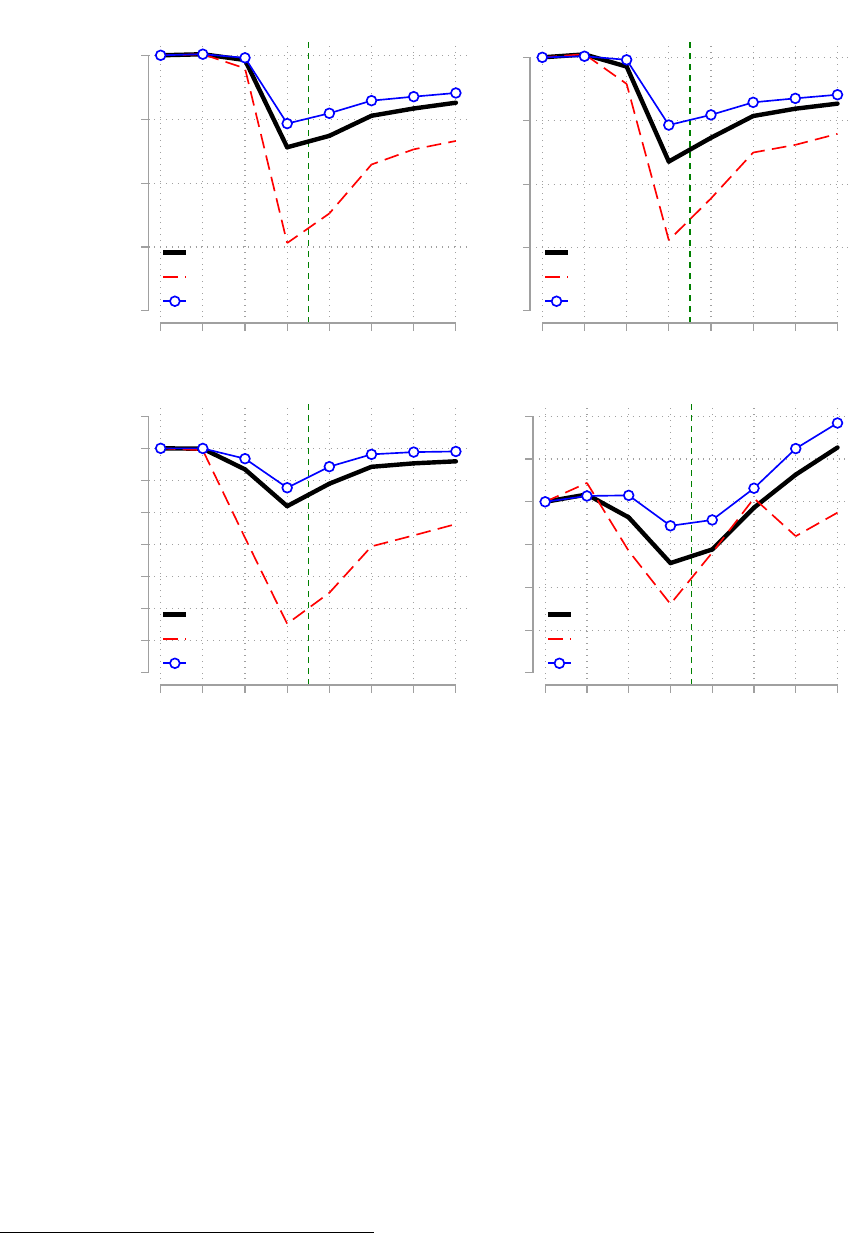
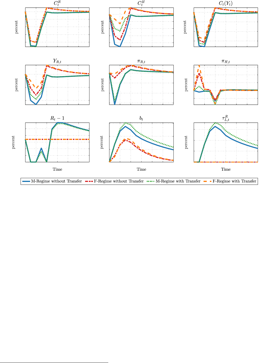
3.3 Quantitative Results
We now present quantitative results on positive and normative implications of redistri-
bution policy during a crisis.
3.3.1 Dynamic Effects of Transfer Policy
We show how key variables evolve over time in response to the COVID shocks—a com-
bination of aggregate and sector-specific demand and supply shocks as discussed above.
We then illustrate the effects of an increase in transfers for the two regimes. These re-
sults are in Figure 2, which presents four different scenarios: the monetary regime with
and without transfers to the HTM households and the fiscal regime with and without
transfers. As mentioned before, we calibrate the COVID shocks to match the targeted
moments under the monetary regime in the absence of transfers. This case thus serves as
our baseline. Throughout, the duration of the redistribution policy is three periods (six
months), which coincides with the duration of the shocks.
25
24
Since the transfer payments from the CARES Act started in mid-April while our calibration strategy
matches model dynamics without transfer policy to the data, there is a slight mismatch between the data
and model counterparts, especially for August.
25
We solve the model non-linearly under perfect foresight. All the model variables converge back to the
steady state in the long run.
24
0 2 4 6 8 10 12
-20
-15
-10
-5
0
0 2 4 6 8 10 12
-8
-6
-4
-2
0
0 2 4 6 8 10 12
-15
-10
-5
0
0 2 4 6 8 10 12
-10
-5
0
0 2 4 6 8 10 12
-6
-4
-2
0
0 2 4 6 8 10 12
-5
0
5
10
15
0 2 4 6 8 10 12
0
0.002
0.004
0.006
0.008
0.01
0 2 4 6 8 10 12
0
10
20
30
0 2 4 6 8 10 12
0
5
10
15
Figure 2: Redistribution Policy with Different Policy Regimes
Notes: This figure shows dynamics of key variables in response to the COVID shocks under different
regimes. Blue solid lines represent the baseline case: the monetary regime without transfers. Red dashed
lines, green dotted lines, and orange dashed lines represent respectively the fiscal regime without trans-
fers, the monetary regime with transfers, and the fiscal regime with transfers.
In the baseline, where the policymakers just stick to the usual policy, the COVID
shocks generate significant short-run contractions in aggregate output and household
consumption of both types, as shown by the solid blue lines in the first row of the fig-
ure. The contraction leads to a decline in inflation (as shown in the second row) and
in labor tax revenues, both of which in turn increase the real value of government debt.
The government responds by increasing the tax rate to stabilize debt under this standard
monetary regime. Meanwhile, the central bank decreases the nominal interest rate in re-
sponse to the decline in inflation. These policy responses are shown in the bottom row of
the figure. Notice that the ZLB binds in our model during the pandemic.
Now, let us introduce the redistribution program to the monetary regime baseline
case, the results of which are shown by the dotted green lines in Figure 2.
26
Overall, the
26
As we discussed in the calibration section, transfers increase by 26.8 percent in total, and here, they are
25

effects of the redistribution program are largely in line with what we have shown using
the simple model in Section 2. One major difference from the simple model is that the
redistribution program is more expansionary here because both the classical labor supply
channel and the Keynesian channel operate thanks to nominal rigidities, as we discussed
in Section 2.3.
Clearly, transfers increase HTM household consumption and decrease Ricardian house-
hold consumption (due to the resulting increase in the tax rate) relative to the baseline.
These are the direct effects of the redistribution. As discussed in Section 2, however, the
redistribution program is inflationary, as shown by the difference between the solid blue
lines and the dotted green lines in the second row. This indirectly has a positive effect on
household consumption of both types through general equilibrium. In particular, the de-
cline of Ricardian household consumption caused by the redistribution is very small, and
in fact in this parameterization it is nearly indistinguishable visually from the baseline
case.
Let us now turn to the fiscal regime where neither the tax rate nor the nominal inter-
est rate changes. The results for this case are shown by the red (without transfers) and
orange (with transfers) lines in Figure 2. The COVID shocks are also contractionary in
this regime, and, moreover, redistribution leads to an increase in HTM consumption as
well as aggregate output.
27
In this fiscal regime, the main aspect we want to highlight
is that aggregate output and consumption of both types do not drop as much as in the
monetary regime. There are three main reasons, which all also help us understand how
the transmission of shocks and transfer policy is different in this regime.
First, irrespective of whether there is redistribution or not, the fiscal regime generates
greater and more persistent inflation than the monetary regime, as that stabilizes the real
value of government debt without relying on labor taxes. Due to nominal rigidities, this
in turn has larger and longer-lasting positive effects on output and consumption of both
types, as presented in the first row of Figure 2. Second, as shown in the simple model
in Section 2.2.2, the redistribution program is more inflationary in the fiscal regime than
in the monetary regime. This result is illustrated in the second row of the figure. The
fifth and sixth panels reveal that the gap between the orange and red lines is greater than
that between the green and blue lines. Finally, the ZLB binds in the monetary regime
as we discussed above, which prevents the central bank from decreasing the policy rate
according to the monetary policy rule, and leads to a bigger drop in the monetary regime
evenly distributed over three periods.
27
In contrast to the monetary regime, redistribution actually increases Ricardian consumption in the fiscal
regime as the aforementioned indirect effect on consumption through inflation dominates the direct effect
in our calibration. This result, however, is difficult to see in the figure. We revisit it in Section 3.3.2.
26

with the shocks. This mechanism is not relevant for the fiscal regime.
3.3.2 Transfer Multipliers
As a way to summarize these dynamic responses with and without redistribution policy,
we now present results in terms of transfer multipliers for output and consumption.
The transfer multiplier for output, for instance, under regime i ∈ {M, F} is defined as
M
i
t
(Y) =
∑
t
h=0
β
h
(
˜
Y
i
h
− Y
M
h
)
∑
t
h=0
β
h
s
h
!
,
where
˜
Y
i
h
is output at horizon h under i-regime with transfers, Y
M
h
is output at horizon
h under the monetary regime without transfers (i.e. the baseline), and s
h
is transfers at
horizon h. The multipliers for Ricardian sector output and the two consumption under i-
regime—denoted respectively by M
i
t
(Y
R
), M
i
t
(C
R
) and M
i
t
(C
H
)—are similarly defined.
Following the government spending multiplier literature, we consider impact multiplier
(t = 0) as well as 2–year (t = 12) and 4–year (t = 24) cumulative multipliers, which
allows for a consideration of dynamic effects in the model.
Note that in calculating these multipliers, our baseline case, as in Section 3.3.1, is al-
ways the monetary regime without transfers. This is the most interesting case to study, as
we want to study the following question: Given a transfer policy we want to implement,
what are the differences if conventional labor taxes or inflation taxes are used to finance
the resulting increase in government debt?
Table 2: Transfer Multipliers
Monetary Regime Fiscal Regime
M
M
t
(Y) M
M
t
(Y
R
) M
M
t
(C
R
) M
M
t
(C
H
) M
F
t
(Y) M
F
t
(Y
R
) M
F
t
(C
R
) M
F
t
(C
H
)
Impact Multipliers 1.175 1.538 -0.205 5.692 3.983 5.272 2.418 9.105
2-Year Cumulative Multipliers 1.154 1.450 -0.217 5.641 7.289 8.884 5.607 12.796
4-Year Cumulative Multipliers 1.126 1.417 -0.244 5.609 7.739 9.408 6.036 13.311
Notes: This table shows the transfer multipliers under the monetary and fiscal regimes. M
i
t
(X) represent the cumulative
transfer multiplier of variable X at t-horizon under i regime. We report impact multipliers (t = 0) as well as 2–year
(t = 12) and 4–year (t = 24) cumulative multipliers when the government distributes transfers evenly over 6 months.
Table 2 shows that aggregate output and Ricardian sector output multipliers are both
above 1 in the monetary regime. The binding ZLB and sticky prices play an important
role in this result.
28
Moreover, the C
H
multiplier is above the simple model benchmark of
(1/λ), which would be 4.35 according to our calibration.
28
In the simple model, we showed analytically that the Ricardian sector output multiplier is below 1.
27

Table 2 also shows that those multipliers are even higher in the fiscal regime, even
though the ZLB is binding in our simulations under the monetary regime. In fact, uniquely,
even the C
R
multiplier is now positive in the fiscal regime, which is different from the
monetary regime.
29
The persistent inflation dynamics in this regime lead to persistent
real effects due to sticky prices, which contributes to these higher multipliers. Later, in
Section 3.4.1, we delve more deeply into the mechanisms that produce such large differ-
ences in the multipliers between the two regimes.
3.3.3 Welfare Effects of Transfer Policy
We finally show the effects on household welfare of the recession created by the COVID
shocks under the four different scenarios discussed above. In particular, we consider
both short- and long-run welfare effects. To this end, we implicitly define our measure of
welfare gain for household of type i ∈ {R, H} , µ
i
t,k
, as
t
∑
j=0
β
j
U
C
i
j
, L
i
j
=
t
∑
j=0
β
j
U
1 + µ
i
t,k
¯
C
i
,
¯
L
i
,
where
¯
C
i
,
¯
L
i
is the steady-state level of type-i household’s consumption and hours,
and
n
C
i
j
, L
i
j
o
are the time path of type-i household’s consumption and hours under the
different transfer duration policies (indexed by k). In this way, µ
i
t,k
measures welfare gains
from period 0 till (arbitrary) period t in units of a percentage of the steady-state (or pre-
COVID) level of consumption—when the redistribution program lasts for k periods.
30
The lifetime (total) welfare gain is then measured by µ
i
∞,k
≡ lim
t→∞
µ
i
t,k
, often the focus
of the business cycle literature. Recall that, unless otherwise noted, we report the case in
which k=3; that is, the duration of the redistribution coincides with the duration of the
shocks.
We find that whether the government introduces the redistribution program and how
it is financed make a very small difference for the lifetime welfare for both types of house-
holds. This result is presented in Table 3. For example, the redistribution program fi-
nanced by inflation taxes, that is the fiscal regime, increases the HTM households’ life-
time welfare by 0.198 percentage point and increases the Ricardian households’ lifetime
welfare by 0.070 percentage point, compared to the baseline. This result is expected be-
cause the COVID shocks under consideration are short-lived, which implies the recession
29
In the simple model where inflation is neutral for real variables, we showed analytically that this mul-
tiplier is negative.
30
It thus measures welfare gains at the point when the agents are t periods, or 2xt months, old since the
initial COVID shocks.
28

Table 3: Welfare Gains
Monetary Regime Fiscal Regime
Transfer Distribution Long-run Short-run
(t = 4)
Long-run Short-run
(t = 4)
Ricardian Household -0.012 -0.819 0.070 1.131
HTM Household 0.074 3.386 0.198 5.600
Notes: This table shows long- and short-run welfare gains resulting from the redistribution, compared to
the baseline. The values are the difference in the welfare measure (µ
i
t,k
) between the transfer cases (under
the two regimes) and the baseline case (the monetary regime without transfers). In the latter case, the
long-run welfare gains for the Ricardian households and for the HTM households are -0.439 and -0.202
percent of the steady-state level of consumption respectively.
is only a small bump in the lifetime.
31
What is more interesting are the welfare effects in the short run, which are presented
in detail in Figure 3. We ask two different, yet related questions. First, taking as given the
redistribution program enacted, what is the better way to finance it? Second, should the
government enact the redistribution policy at all?
On the first question, we find that, taking the redistribution program as given, infla-
tion taxes, as used in the fiscal regime, produce far better welfare outcomes than labor
taxes, as used in the monetary regime. For example, at the point when the pandemic is
over (at t = 4), as given in Table 3, the redistribution program, financed by inflation taxes
(i.e., the fiscal regime), would have increased the welfare of the HTM households and
that of the Ricardian households by 5.6 percentage points and 1.131 percentage points,
respectively, compared to the baseline. This result on the welfare gains under the fiscal
regime can be inferred from the second and third panels of Figure 3.
32
In contrast, if
the government relied on labor taxes, the HTM households’ welfare gain resulting from
the redistribution would amount to 3.386 percentage points of the steady-state level of
consumption at the end of the pandemic. Therefore, labor-tax financed transfers are less
effective. Moreover, the redistribution now decreases the welfare of the Ricardian house-
holds by 0.819 percentage point, as these households work more hours with little change
in consumption.
We now consider the second question—that is, whether the redistribution policy is de-
sirable at all. The answer is obviously that it depends. Figure 3 shows that the inflation-
financed redistribution program under the fiscal regime benefits the HTM households the
31
We shut down all shocks other than the three-period COVID shocks over the lifetime. Therefore, this
exercise is different from the usual ones in the business cycle literature.
32
Specifically, the welfare improvements over the baseline case can be obtained by taking the difference
between the orange lines and the blue lines (the baseline).
29
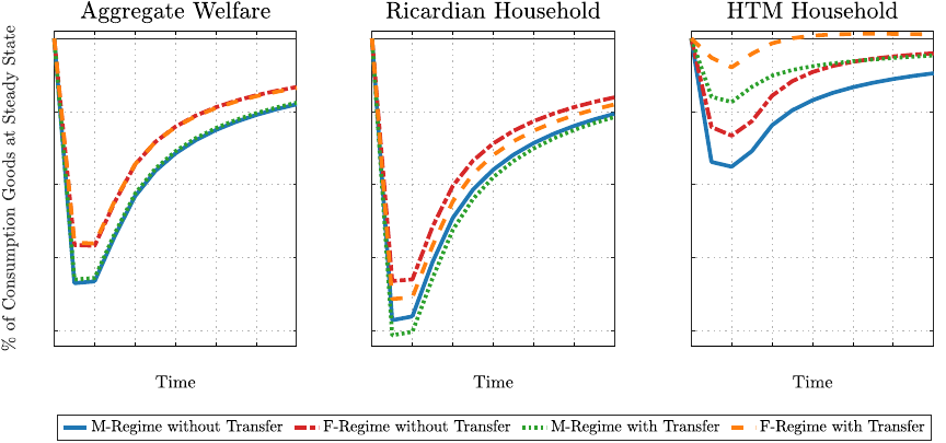
0 2 4 6 8 10 12
-20
-15
-10
-5
0
0 2 4 6 8 10 12
-20
-15
-10
-5
0
0 2 4 6 8 10 12
-20
-15
-10
-5
0
Figure 3: Short-Run Welfare Gains Comparison
Notes: This figure presents the short-run welfare gains under the four different scenarios, showing µ
i
t,k
as a function of t. The numbers are in units of a percentage of the steady-state level of consumption.
most, but it is not the best option for the Ricardian households. But if the policy objec-
tive was simply to maximize the aggregate welfare, which is not likely the most realistic
case, the redistribution program by itself would do very little given the policy regime in
this model, as shown in the first panel of Figure 3. With transfer payments, in either
policy regime, the HTM households would consume more, which would also lead to an
increase in aggregate output. At the same time, the Ricardian households would have to
work more for two reasons. The first reason is to produce more output. The second rea-
son is that inflation created by the redistribution generates resource misallocation, which
increases labor hours required to produce a given amount of output, as shown in Equa-
tion (3.1). In our calibration here, these two welfare effects almost cancel each other out
in both regimes.
3.4 Extensions and Sensitivity Analysis
We now consider some important extensions and sensitivity analysis.
3.4.1 Inspecting the Mechanisms of Transfer Multipliers
As our main extension, we do several exercises to inspect the mechanisms that drive
transfer multipliers across the two regimes. First, we decompose the transfer multiplier
into three different components in Table 4, where in this decomposition, the output mul-
30

tiplier, for instance, under regime i ∈ {M, F} is
M
i
t
(Y) =
∑
t
h=0
β
h
(
˜
Y
i
h
−
˜
Y
i
no shock,h
)
∑
t
h=0
β
h
s
h
!
| {z }
COVID Effect with Transfer
+
∑
t
h=0
β
h
(
˜
Y
i
no shock,h
−
¯
Y)
∑
t
h=0
β
h
s
h
!
| {z }
Transfer Effect without COVID Shocks
−
∑
t
h=0
β
h
(Y
M
h
−
¯
Y)
∑
t
h=0
β
h
s
h
!
| {z }
COVID Effect without Transfer
(3.2)
where
˜
Y
i
h
is output at horizon h under i-regime with both transfers and COVID shocks,
˜
Y
i
no shock,h
is output at horizon h under i-regime with transfers, but without COVID shocks,
Y
M
h
is output at horizon h under the monetary regime with COVID shocks, but without
transfers,
¯
Y is output at steady-state, and s
h
is transfers at horizon h. Note that the third
effect is the same across regimes, while the first two are different as they compute the
effect for a given regime.
Table 4: Transfer Multipliers Decomposition
Monetary Regime Fiscal Regime
M
M
t
(Y) M
M
t
(Y
R
) M
M
t
(C
R
) M
M
t
(C
H
) M
F
t
(Y) M
F
t
(Y
R
) M
F
t
(C
R
) M
F
t
(C
H
)
Panel A: Impact Multipliers
Total Effect 1.175 1.538 -0.205 5.692 3.983 5.272 2.418 9.105
COVID Effect with Transfer -14.982 -6.446 -16.435 -10.226 -12.920 -3.589 -14.523 -7.671
Transfer Effect without COVID 0.742 0.867 -0.597 5.125 1.488 1.743 0.115 5.984
COVID Effect without Transfer -15.415 -7.117 -16.827 -10.793 -15.415 -7.117 -16.827 -10.793
Panel B: 2-Year Cumulative Multipliers
Total Effect 1.154 1.450 -0.217 5.641 7.289 8.884 5.607 12.796
COVID Effect with Transfer -14.161 -8.455 -15.090 -11.123 -8.493 -1.568 -9.711 -4.504
Transfer Effect without COVID 1.007 1.178 -0.344 5.430 1.474 1.725 0.101 5.967
COVID Effect without Transfer -14.308 -8.727 -15.217 -11.333 -14.308 -8.727 -15.217 -11.333
Panel C: 4-Year Cumulative Multipliers
Total Effect 1.126 1.417 -0.244 5.609 7.739 9.408 6.036 13.311
COVID Effect with Transfer -14.655 -9.030 -15.561 -11.688 -8.557 -1.643 -9.773 -4.578
Transfer Effect without COVID 0.960 1.123 -0.389 5.376 1.475 1.727 0.103 5.968
COVID Effect without Transfer -14.821 -9.324 -15.707 -11.921 -14.821 -9.324 -15.707 -11.921
Notes: This table shows the decomposition of the transfer multipliers for aggregate output, Ricardian sector output, Ricardian
consumption and HTM consumption, as given in Equation (3.2). M
i
t
(X) represent the cumulative transfer multiplier of variable
X at t-horizon under i regime. We report impact multipliers (t = 0) as well as 2–year (t = 12) and 4–year (t = 24) cumulative
multipliers.
As Table 4 shows, even without the COVID shocks, the transfer multipliers are higher
in the fiscal regime. This result is captured by the second component in Equation (3.2).
For example, this component of the impact multiplier for output is 1.488 under the fiscal
regime, while it is only 0.742 under the monetary regime. Moreover, uniquely in the fiscal
regime, the Ricardian consumption multiplier is positive (e.g. 0.115 on impact). The main
reason for these results is the high and persistent effects on inflation in the fiscal regime
induced by an increase in transfer, as shown in our analytical analysis.
31

We now consider the state-dependence of the transfer multipliers, first within and
then across the regimes. First, in each of the two regimes, the transfer multipliers condi-
tional on no COVID shocks (i.e. the second component) are less than the total multipliers.
In the absence of the COVID shocks—that is, if the economy were in the steady state—
transfer-induced inflation, while boosting the economy, would also generate inefficient
price dispersion, which in turn would lead to resource misallocations and decrease labor
productivity. However, if the economy were already in a COVID-recession, inflation-
ary pressures resulting from redistribution would actually counteract deflation due to the
COVID shocks, thereby decreasing, rather than increasing, the extent of such price dis-
persion. In addition, in the case of monetary regime, the ZLB is irrelevant with no COVID
shocks, which means that transfer-induced inflationary pressures do not lead to as strong
a boost in consumption as the real interest rate does not decrease strongly.
Second, comparing the two regimes, the transfer multipliers are more state-dependent
in the fiscal regime than in the monetary regime. That is, transfers are disproportionately
more effective in the fiscal regime than in the monetary regime when the economy falls
into a COVID-recession. The reason is that the aforementioned "counteracting" force is
much stronger in the fiscal regime that produces higher and more persistent inflation.
33
Table 4 shows that the large difference in the multipliers between the two regimes is
driven quantitatively by the first component, which captures how the effectiveness of
transfers depends on the presence of COVID shocks. This is a measure of state depen-
dence.
Besides the state dependence, our quantitative model includes two additional features
that break the uniformity—obtained in the simple, analytical model—of the two regimes
in terms of the multipliers. They are nominal rigidities and distortionary labor taxes. In
order to isolate the role of these two features, we delve more into the second component
of the transfer multipliers in Equation (3.2) through counterfactual exercises.
For reference, Panel A of Table 5 first re-reports the second component in the presence
of the two features.
34
We then remove nominal rigidities (in Panel B) and further remove
distortionary labor taxes (in Panel C). The last version then is quite close to our simple,
analytical model. This exercise thus progressively allows an analysis of which elements
are responsible for differences between the simple and the quantitative model results—
besides the COVID shocks.
Panel B of Table 5 shows that the multipliers decrease substantially with flexible prices,
33
We can see this in the fifth panel of Figure 2. Without transfer, as shown by the blue line, the COVID
shocks generate a significant deflation, which can be undone by inflation-financed transfers (shown by the
orange line).
34
The values in the panel are thus the same as those in the third row of each panel of Table 4
32

Table 5: Transfer Multipliers without COVID Shocks
Monetary Regime Fiscal Regime
M
M
t
(Y) M
M
t
(Y
R
) M
M
t
(C
R
) M
M
t
(C
H
) M
F
t
(Y) M
F
t
(Y
R
) M
F
t
(C
R
) M
F
t
(C
H
)
Panel A: Without COVID Shocks under sticky price
Impact Multipliers 0.742 0.867 -0.597 5.125 1.488 1.743 0.115 5.984
2-Year Cumulative Multipliers 1.007 1.178 -0.344 5.430 1.474 1.725 0.101 5.967
4-Year Cumulative Multipliers 0.960 1.123 -0.389 5.376 1.475 1.727 0.103 5.968
Panel B: Without COVID Shocks under flexible price
Impact Multipliers 0.465 0.543 -0.861 4.807 0.465 0.543 -0.861 4.807
2-Year Cumulative Multipliers 0.214 0.251 -1.101 4.520 0.465 0.543 -0.861 4.807
4-Year Cumulative Multipliers 0.095 0.111 -1.215 4.383 0.465 0.543 -0.861 4.807
Panel C: Without COVID Shocks under flexible price and lump-sum tax adjustment
Impact Multipliers 0.465 0.543 -0.861 4.807 0.465 0.543 -0.861 4.807
2-Year Cumulative Multipliers 0.465 0.543 -0.861 4.807 0.465 0.543 -0.861 4.807
4-Year Cumulative Multipliers 0.465 0.543 -0.861 4.807 0.465 0.543 -0.861 4.807
Notes: This table shows the transfer multipliers without COVID shocks. Panel A reports multipliers under sticky prices
and distortionary labor taxes. Panels B reports multipliers under flexible prices and distortionary labor taxes. Panels
C reports multipliers under flexible prices and non-distortionary lump-sum taxes. M
i
t
(X) represent the cumulative
transfer multiplier of variable X at t-horizon under i regime. We report impact multipliers (t = 0), 2–year (t = 12), and
4–year (t = 24) cumulative multipliers.
as is often also found in the government spending multiplier literature. In fact, now
the impact multipliers are the same across the regimes, as was the case in our simple,
analytical model, as different inflation dynamics do not affect real allocations. Moreover,
output multipliers are now below 1, the Ricardian consumption multiplier is negative,
and the HTM consumption multiplier is close to 4.35, the analytical model solution.
35
The
cumulative multipliers are different from the impact multiplier in the monetary regime—
unlike the simple, analytical model—due to dynamics of distortionary labor taxes.
To make this clear, Panel C of Table 5 shows the case where the increase in transfers
are financed by lump-sum taxes on the Ricardian household. Then, all the multipliers are
the same across the regimes and over horizons, as in the simple, analytical model.
3.4.2 Sensitivity Analysis
As our first sensitivity exercise, we do additional analysis related to the length of the
transfer policy. So far, transfer policy duration coincided with the length of the COVID
shocks—that is, six months. We now show results for three different durations of redistri-
35
The solution for multipliers in the simple model that we derive would predict a Ricardian sector output
multiplier of 0.644 and Ricardian consumption multiplier of -0.464. Note that the simple model imposes
log utility and is also a one-sector environment.
33

bution policy: The program lasts for 2, 6, and 12 months. This exercise can be important,
as our model features HTM households. Moreover, the timing of transfers can also matter
because there are distortionary labor taxes in the model and also when the economy is at
ZLB under the monetary regime. For the different durations of the program, we fix the
present value of transfers to be the same, which implies that the amount of transfers each
period is smaller when the program lasts longer.
Appendix Figures B.1 and B.2 present the responses of the variables with different du-
ration of the redistribution program under the monetary and fiscal regimes, respectively.
We find that the results are overall quite similar across different lengths of the redistribu-
tion policy, except for the responses of HTM household consumption. The second panel
of the figures shows that the difference in HTM household consumption between the no-
transfer and transfer cases, for obvious reasons, is more evenly distributed across time
periods when the duration of the program is longer. Appendix Table B.2 presents the
multiplier results under different duration of transfer policy. The multipliers are higher
under the monetary regime when transfer is distributed over a longer duration. For the
fiscal regime, the cumulative multipliers, which capture dynamics in the model, are rela-
tively insensitive to the duration of transfer policy.
36
We next do sensitivity analysis with respect to two assigned parameters. We first con-
sider a cross-sector elasticity of substitution (ε) greater than 1, equal to 1.2. Our baseline
parameterization was 0.8. Next, we consider a different parameterization of the tax rule
response coefficient (ψ
L
) under the M regime. Compared to our baseline choice of 0.6,
we now set it at 0.1, such that labor tax rates respond less strongly to debt.
37
In these
exercises, we keep the rest of the parameters the same as the baseline.
38
Appendix Figure B.3 presents the responses of the variables with and without transfer
policy when ε = 1.2, while Table B.4 presents the transfer multipliers when ε = 1.2.
Overall, the results are similar to our baseline results. One noticeable difference is that as
the sectoral goods are more substitutable now, the consumption multiplier for the HTM
household is lower while that for the Ricardian household is higher.
Appendix Figure B.4 present the responses of the variables with and without transfer
policy when ψ
L
= 0.1 under the monetary regime, while Appendix Table B.5 presents
the transfer multipliers when ψ
L
= 0.1. The results are very similar to our baseline re-
sults. One noticeable difference is that as labor tax rates increase less strongly, under the
36
Appendix Table B.3 presents welfare results. Consistent with the multiplier results, in the monetary
regime, the longer duration transfer policy leads to welfare improvement for both the households.
37
This is in line with the estimates in Bhattarai, Lee and Park (2016), which however did not have distor-
tionary labor taxes.
38
These different sensitivity analysis exercises thus will not match the targeted moments anymore.
34

monetary regime, the multipliers are somewhat higher.
39
Finally, Appendix Table B.6 presents the transfer multipliers when we exclude $600
individual tax rebates in the CARES Act from our transfer experiment. The main motiva-
tion is the survey finding in Coibion, Gorodnichenko and Weber (2020) that on average,
only about 40% of tax rebates appears to have been spent by households. The size of
transfer change decreases from 26.8% to 15.7% when we exclude the individual tax re-
bates.
40
Table B.6 shows that the multipliers are essentially the same as before under the
monetary regime. For the fiscal regime however, the multipliers are even bigger. This is
another example of state dependence of multipliers, where the results differ by the size
of the change in transfers. The decomposition shows that this is driven by the higher
marginal effectiveness of transfers with COVID shocks in this regime.
4 Conclusion
Our paper makes clear that how transfers are ultimately financed is a first-order issue for
their effectiveness. It arguably matters more than other factors identified in the literature,
which typically reports moderate transfer multipliers. We show that inflation-financed
transfers are significantly more effective than tax-financed transfers in boosting the econ-
omy and improving welfare. Such an inflation-financed transfer program can be imple-
mented by a fiscal authority committing itself to no tax adjustments in the foreseeable fu-
ture, coupled with an accommodative monetary authority. We call such a fiscal-monetary
policy mix the fiscal regime—in contrast to the (conventional) monetary regime where
monetary policy stabilizes inflation.
We first consider a simple two-agent model that permits analytical results and illumi-
nates the mechanism through which redistribution generates inflation in the two policy
regimes. In particular, the fiscal regime produces high and persistent inflation through
the direct and the indirect (that we also called the interest rate or valuation) channels. In
comparison, inflation is lower and shorter lived in the monetary regime. We then build
on the analytical results and proceed to a quantitative analysis in a two-sector extension.
Our quantitative exercise shows that inflation-financed transfers fight deflationary pres-
sures in a COVID-recession-like environment, thereby preventing output and consump-
tion from dropping significantly. Such inflation-induced expansionary effects are so large
39
For the fiscal regime, the only reason the multiplier results are different from our baseline is that the
monetary regime under no transfers now has different dynamics.
40
Other than changing the size of the transfer increase, this does not affect our parameterization as we
calibrate the economy in the absence of transfer policy.
35

that redistribution can in fact produce a Pareto improvement.
In future work, we can take additional steps in several directions. First, the model may
be extended to feature a richer form of heterogeneity across sectors as well as households
and, in addition, more elaborate matching between sectors and households. Although
we expect that our main argument will hold in such a complex environment, it will be
interesting to see whether such an extension affects the quantitative results significantly.
Second, while our analysis suggests a clear path for the success of a redistribution policy,
the Great Recession taught policymakers that generating inflation during, and in the after-
math of, a severe recession is easier said than done, possibly due to credibility problems.
Relatedly, implementation would not be as straightforward in an environment where eco-
nomic agents take into account the possibility of regime switching by policymakers when
the recession is over, as suggested in this paper. We leave a more comprehensive analysis
of such interesting issues for future research.
References
Bassetto, Marco, “A Game-Theoretic View of the Fiscal Theory of the Price Level,” Econo-
metrica, 2002, 70 (6), 2167–2195.
Bayer, Christian, Benjamin Born, Ralph Luetticke, and Gernot Müller, “The Coron-
avirus Stimulus Package: How Large is the Transfer Multiplier?,” CEPR Discussion
Papers 14600, C.E.P.R. Discussion Papers 2020.
Bhattarai, Saroj, Jae Won Lee, and Woong Yong Park, “Inflation Dynamics: The Role of
Public Debt and Policy Regimes,” Journal of Monetary Economics, 2014, 67, 93–108.
, , and , “Policy Regimes, Policy Shifts, and U.S. Business Cycles,” The Review of
Economics and Statistics, 2016, 98 (5), 968–83.
, , , and Choongryul Yang, “Macroeconomic Effects of Capital Tax Rate Changes,”
Globalization and Monetary Policy Institute Working Paper 391 2020.
Bianchi, Francesco, Renato Faccini, and Leonardo Melosi, “Monetary and Fiscal Policies
in Times of Large Debt: Unity is Strength,” NBER Working Papers 27112, National
Bureau of Economic Research, Inc May 2020.
Bilbiie, Florin O., “Monetary Policy and Heterogeneity: An Analytical Framework,”
CEPR Discussion Paper DP12601 2018.
36

, Tommaso Monacelli, and Roberto Perotti, “Public Debt and Redistribution with Bor-
rowing Constraints,” The Economic Journal, 2013, 123 (566), F64–F98.
Campbell, John Y. and N. Gregory Mankiw, “Consumption, Income, and Interest Rates:
Reinterpreting the Time Series Evidence,” NBER Macroeconomics Annual, 1989, 4, 185–
216.
Canzoneri, Matthew, Robert Cumby, and Behzad Diba, “The Interaction Between Mon-
etary and Fiscal Policy,” in Benjamin M. Friedman and Michael Woodford, eds., Hand-
book of Monetary Economics, Vol. 3, Elsevier, 2010, pp. 935–999.
Christiano, Lawrence, Martin Eichenbaum, and Sergio Rebelo, “When Is the Govern-
ment Spending Multiplier Large?,” Journal of Political Economy, 2011, 119 (1), 78–121.
Cochrane, John H., “Long-Term Debt and Optimal Policy in the Fiscal Theory of the Price
Level,” Econometrica, 2001, 69 (1), 69–116.
, “Michelson-Morley, Fisher, and Occam: The Radical Implications of Stable Quiet In-
flation at the Zero Bound,” NBER Macroeconomics Annual, 2018, 32, 113–226.
Coibion, Olivier, Yuriy Gorodnichenko, and Michael Weber, “How Did U.S. Con-
sumers Use Their Stimulus Payments?,” Working Paper 27693, National Bureau of Eco-
nomic Research August 2020.
Del Negro, Marco, Marc P. Giannoni, and Frank Schorfheide, “Inflation in the Great
Recession and New Keynesian Models,” American Economic Journal: Macroeconomics,
January 2015, 7 (1), 168–96.
Eggertsson, Gauti B., “What Fiscal Policy Is Effective at Zero Interest Rates?,” NBER
Macroeconomics Annual, 2011, 25, 59–112.
Faria-e-Castro, Miguel, “Fiscal Policy during a Pandemic,” Working Papers 2020-006,
Federal Reserve Bank of St. Louis 2020.
Galí, Jordi, J. David López-Salido, and Javier Vallés, “Understanding the Effects of Gov-
ernment Spending on Consumption,” Journal of the European Economic Association, 2007,
5 (1), 227–70.
Guerrieri, Veronica, Guido Lorenzoni, Ludwig Straub, and Iván Werning, “Macroeco-
nomic Implications of COVID-19: Can Negative Supply Shocks Cause Demand Short-
ages?,” Working Paper 26918, National Bureau of Economic Research April 2020.
37

Hall, Robert E, “New Evidence on the Markup of Prices over Marginal Costs and the
Role of Mega-Firms in the US Economy,” Working Paper 24574, National Bureau of
Economic Research May 2018.
Hobijn, Bart and Fernanda Nechio, “Sticker Shocks: Using VAT Changes to Estimate
Upper-Level Elasticities of Substitution,” Journal of the European Economic Association,
04 2018, 17 (3), 799–833.
Jacobson, Margaret M., Eric M. Leeper, and Bruce Preston, “Recovery of 1933,” NBER
Working Papers 25629, National Bureau of Economic Research, Inc March 2019.
Leeper, Eric M., “Equilibria under ’Active’ and ’Passive’ Monetary and Fiscal Policies,”
Journal of Monetary Economics, 1991, 27 (1), 129–47.
and Campbell Leith, “Understanding Inflation as a Joint Monetary-Fiscal Phe-
nomenon,” in John B. Taylor and Harald Uhlig, eds., Handbook of Macroeconomics, Vol. 2,
Elsevier, 2016, chapter 30, pp. 2305–2415.
, Nora Traum, and Todd B. Walker, “Clearing Up the Fiscal Multiplier Morass,” Amer-
ican Economic Review, August 2017, 107 (8), 2409–54.
Motyovszki, Gergo, “Monetary-Fiscal Interactions and Redistribution in Small Open
Economies,” EUI Working Papers 2020/03, ECO 2020.
Schmitt-Grohé, Stephanie and Martín Uribe, “Price Level Determinacy and Monetary
Policy under a Balanced-Budget Requirement,” Journal of Monetary Economics, 2000, 45
(1), 211–246.
Sims, Christopher A., “A Simple Model for Study of the Determination of the Price Level
and the Interaction of Monetary and Fiscal Policy,” Economic Theory, 1994, 4 (3), 381–99.
, “Stepping on a Rake: The Role of Fiscal Policy in the Inflation of the 1970s,” European
Economic Review, 2011, 55 (1), 48–56.
Woodford, Michael, “Monetary Policy and Price Level Determinacy in a Cash-in-
Advance Economy,” Economic Theory, 1994, 4 (3), 345–80.
, “Simple Analytics of the Government Expenditure Multiplier,” American Economic
Journal: Macroeconomics, 2011, 3 (1), 1–35.
38
APPENDIX
A Data Appendix
Employment and Total Hours. We use total employment and total hours data from
U.S. Bureau of Labor Statistics. We define HTM sector as the sum of the following three
sectors: Retail Trade (NAICS 44–45), Transportation and Warehousing (NAICS 48–49),
and Leisure and Hospitality (NAICS 71–72).
Consumption and Inflation. We use real Personal Consumption Expenditure (PCE)
data and PCE inflation from U.S. Bureau of Economic Analysis. We define HTM sec-
tor as the sum of the following three sectors: Transportation services, Recreation services,
and Food services and accommodations.
We also use 2019 Consumer Expenditure Surveys (CEX) data to calibrate both Ricar-
dian and HTM households’ share parameters in the consumption baskets. We assume
households in the top 80 percentile income distribution as Ricardian households and
match their consumption share for transportation, entertainment, and food away from
home. Similarly, we assume households in bottom 20 percentile income distribution as
HTM households and match their consumption share for these three sectors.
Fiscal Variables. We use government current transfer payments (A084RC1Q027SBEA
in FRED) to calibrate steady-state transfers to GDP ratio. We also use federal debt held
by the public data (FYGFDPUN in FRED) to calibrate debt to GDP ratio. Finally, we
use compensation of employees, paid: wages and salaries (A4102C1Q027SBEA in FRED),
proprietors’ income (PROPINC in FRED), and federal government current receipts: con-
tributions for government social insurance (W780RC1Q027SBEA in FRED) data to cali-
brate steady-state labor tax revenue to GDP ratio. The sample period for these variables
is from 1990Q1 through 2020Q1.
Transfer Distribution from CARES Act. We calibrate the size of transfer distribution
using the transfer amounts specified in Coronavirus Aid, Relief and Economy Security
Act (CARES Act), which came into operation in mid–April. In particular, we target the
sum of three key components of the Act: $293 billion to provide one-time tax rebates to
individuals; (ii) $268 billion to expand unemployment benefits; (iii) $150 billion in trans-
fers to state and local governments. These three components of the CARES Act consist of
around 3.4 percent of GDP. In a sensitivity analysis, we count only components (ii) and
(iii) above.
39

B Appendix Tables and Figures
Appendix Table B.1: Data and Model Moments
Time Data Model
Panel A: Targeted moments (percent deviation from January)
Total Hours for retail, transportation, leisure/hospitality April -16.7% -16.7%
June -18.8% -18.8%
August -13.2% -13.2%
Total Hours excluding retail, transportation, leisure/hospitality April -6.58% -6.58%
June -8.57% -8.57%
August -6.13% -6.13%
PCE Inflation for recreation, transportation, food services April -0.99% -0.99%
June -0.39% -0.39%
August -0.37% -0.37%
Panel B: Non-targeted moments (percent deviation from January)
PCE Inflation excluding recreation, transportation, food services April -0.14% -6.30%
June -0.06% -2.29%
August 0.74% -0.12%
Real PCE for recreation, transportation, food services April -41.1% -16.7%
June -37.6% -18.8%
August -25.2% -13.2%
Real PCE excluding recreation, transportation, food services April -7.74% -9.98%
June -3.78% -11.6%
August -1.06% -8.69%
Real GDP (percent deviation from Q1) Q2 -8.99% -12.8%
Q3 -2.25% -0.07%
Notes: This table shows moments of the data and simulated series from the baseline model parameterized at the
values in Table 1. Panel A shows targeted moments and Panel B shows non-targeted moments. Data moments are
expressed as the percent deviation from the average values of outcome variables in January and February.
40

Appendix Table B.2: Multipliers with Different Transfer Distribution
Monetary Regime Fiscal Regime
Transfer Duration k = 1 k = 3 k = 6 k = 1 k = 3 k = 6
Panel A: Impact multiplier
M
i
0
(Y) 1.074 1.175 1.862 2.047 3.983 6.799
M
i
0
(Y
R
) 1.417 1.538 2.434 2.732 5.272 8.979
M
i
0
(C
R
) -0.301 -0.205 0.439 0.606 2.418 5.053
M
i
0
(C
H
) 5.575 5.692 6.520 6.766 9.105 12.514
Panel B: 2-year cumulative multiplier
M
i
12
(Y) 1.072 1.154 1.718 7.323 7.289 7.121
M
i
12
(Y
R
) 1.414 1.450 2.080 8.998 8.884 8.629
M
i
12
(C
R
) -0.303 -0.217 0.326 5.630 5.607 5.453
M
i
12
(C
H
) 5.572 5.641 6.277 12.865 12.796 12.578
Panel C: 4-year cumulative multiplier
M
i
24
(Y) 1.035 1.126 1.749 7.778 7.739 7.550
M
i
24
(Y
R
) 1.371 1.417 2.116 9.528 9.408 9.130
M
i
24
(C
R
) -0.338 -0.244 0.355 6.065 6.036 5.863
M
i
24
(C
H
) 5.530 5.609 6.312 13.386 13.311 13.070
Notes: This table shows the transfer multipliers with different duration of transfer distribution under
different regimes (monetary and fiscal regimes). M
i
t
(X) represent the cumulative transfer multiplier of
variable X at t-horizon under i regime. Panel A shows impact multipliers and Panels B and C present
two-year and four-year cumulative multipliers, respectively. We consider three cases of different dura-
tion of transfer distribution: 2-month (k = 1), 6-month (k = 3), and 12-month (k = 6).
Appendix Table B.3: Long-run Welfare Gains
Monetary Regime Fiscal Regime
Transfer Duration k = 1 k = 3 k = 6 k = 1 k = 3 k = 6
Ricardian Household -0.011 -0.012 -0.002 0.079 0.070 0.063
HTM Household 0.048 0.074 0.090 0.172 0.198 0.202
Notes: This table shows the long-run welfare gains for the models with different regimes and horizons of
transfer distributions. The numbers represent the percentage point deviations from the welfare gains
under monetary regime without transfers. We consider three cases of different duration of transfer
distribution: 2-month (T = 1), 6-month (T = 3), and 12-month (T = 6).
41

Appendix Table B.4: Transfer Multipliers (k = 3, ε = 1.2)
Monetary Regime Fiscal Regime
M
M
t
(Y) M
M
t
(Y
R
) M
M
t
(C
R
) M
M
t
(C
H
) M
F
t
(Y) M
F
t
(Y
R
) M
F
t
(C
R
) M
F
t
(C
H
)
Impact Multipliers 1.086 1.262 -0.105 4.983 5.222 6.119 4.474 7.671
2-Year Cumulative Multipliers 1.072 1.220 -0.123 4.983 9.306 10.475 8.951 10.469
4-Year Cumulative Multipliers 1.044 1.189 -0.153 4.964 9.885 11.112 9.588 10.859
Notes: This table shows the transfer multipliers for the models under monetary and fiscal regimes when ε = 1.2. M
i
t
(X)
represent the cumulative transfer multiplier of variable X at t-horizon under i regime. We report impact multipliers,
two-year, and four-year cumulative multipliers when government distributes transfers equally over 6 months.
Appendix Table B.5: Transfer Multipliers (k = 3, ψ
L
= 0.1 )
Monetary Regime Fiscal Regime
M
M
t
(Y) M
M
t
(Y
R
) M
M
t
(C
R
) M
M
t
(C
H
) M
F
t
(Y) M
F
t
(Y
R
) M
F
t
(C
R
) M
F
t
(C
H
)
Impact Multipliers 1.184 1.549 -0.196 5.703 4.023 5.324 2.456 9.154
2-Year Cumulative Multipliers 1.262 1.577 -0.114 5.766 6.957 8.497 5.290 12.415
4-Year Cumulative Multipliers 1.262 1.577 -0.114 5.766 7.363 8.971 5.677 12.881
Notes: This table shows the transfer multipliers for the models under monetary and fiscal regimes when ψ
L
= 0.1. M
i
t
(X)
represent the cumulative transfer multiplier of variable X at t-horizon under i regime. We report impact multipliers, two-
year, and four-year cumulative multipliers when government distributes transfers equally over 6 months.
Appendix Table B.6: Transfer Multipliers (k = 3, Excluding $600 Individual Tax Rebates)
Monetary Regime Fiscal Regime
M
M
t
(Y) M
M
t
(Y
R
) M
M
t
(C
R
) M
M
t
(C
H
) M
F
t
(Y) M
F
t
(Y
R
) M
F
t
(C
R
) M
F
t
(C
H
)
Panel A: Impact Multipliers
Total Effect 1.173 1.532 -0.206 5.689 5.775 7.625 4.096 11.272
COVID Effect with Transfer -25.878 -11.478 -28.329 -17.855 -22.039 -6.278 -24.755 -13.148
Transfer Effect without COVID 0.738 0.862 -0.601 5.120 1.500 1.754 0.127 5.996
COVID Effect without Transfer -26.314 -12.149 -28.724 -18.423 -26.314 -12.149 -28.724 -18.423
Panel B: 2-Year Cumulative Multipliers
Total Effect 1.154 1.448 -0.216 5.641 11.376 13.807 9.490 17.549
COVID Effect with Transfer -24.280 -14.629 -25.850 -19.139 -14.546 -2.840 -16.610 -7.790
Transfer Effect without COVID 1.010 1.180 -0.341 5.433 1.498 1.751 0.124 5.993
COVID Effect without Transfer -24.424 -14.897 -25.975 -19.346 -24.424 -14.897 -25.975 -19.346
Panel C: 4-Year Cumulative Multipliers
Total Effect 1.127 1.415 -0.242 5.609 12.172 14.735 10.251 18.463
COVID Effect with Transfer -25.136 -15.627 -26.668 -20.12 -14.631 -2.939 -16.691 -7.887
Transfer Effect without COVID 0.963 1.125 -0.386 5.379 1.504 1.758 0.130 6.000
COVID Effect without Transfer -25.299 -15.917 -26.811 -20.350 -25.299 -15.917 -26.811 -20.350
Notes: This table shows the transfer multipliers for the models under monetary and fiscal regimes when we exclude $600 individual
tax rebates from our transfer experiment. The total value of transfer distribution to GDP ratio decreases from 26.8% to 15.7% when we
exclude the individual tax rebates. M
i
t
(X) represent the cumulative transfer multiplier of variable X at t-horizon under i regime. We
report impact multipliers, 2-year, and 4-year cumulative multipliers when government distributes transfers equally over 6 months.
42
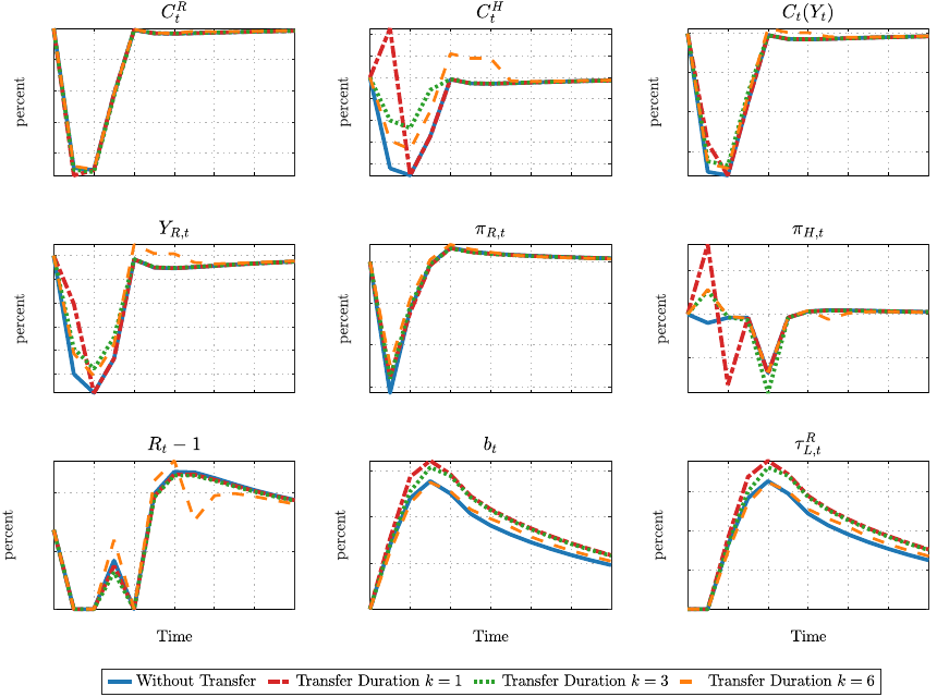
0 2 4 6 8 10 12
-20
-15
-10
-5
0
0 2 4 6 8 10 12
-8
-6
-4
-2
0
2
4
0 2 4 6 8 10 12
-15
-10
-5
0
0 2 4 6 8 10 12
-10
-8
-6
-4
-2
0
0 2 4 6 8 10 12
-6
-4
-2
0
0 2 4 6 8 10 12
-5
0
5
0 2 4 6 8 10 12
0
0.005
0.01
0 2 4 6 8 10 12
0
10
20
30
0 2 4 6 8 10 12
0
5
10
15
Appendix Figure B.1: Monetary Regime: Different Duration of Redistribution Policy
Notes: This figure shows dynamics of key variables in response to the COVID shocks under monetary
regime with different duration of transfer distribution. Blue solid lines represent the baseline model
without transfers. Red dashed lines represent the case of one-time transfer distribution. Green dotted
lines represent the case where the transfers are distributed over three-period (6 months) and orange
dashed lines represent the case where the transfers are distributed over six-period (12 months). We set
the total present value of transfer amounts are the same across different duration of distribution policy.
43
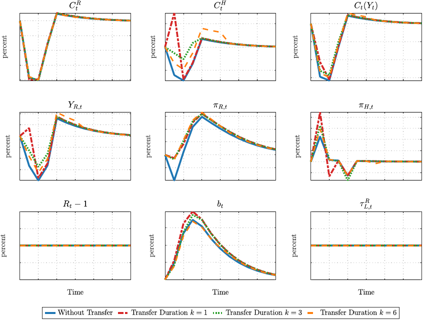
0 2 4 6 8 10 12
-20
-15
-10
-5
0
0 2 4 6 8 10 12
-5
0
5
0 2 4 6 8 10 12
-15
-10
-5
0
0 2 4 6 8 10 12
-6
-4
-2
0
2
4
0 2 4 6 8 10 12
-0.5
0
0.5
1
1.5
0 2 4 6 8 10 12
-5
0
5
10
15
20
0 2 4 6 8 10 12
-0.5
0
0.5
1
0 2 4 6 8 10 12
0
5
10
15
0 2 4 6 8 10 12
-1
-0.5
0
0.5
1
Appendix Figure B.2: Fiscal Regime: Different Duration of Redistribution Policy
Notes: This figure shows dynamics of key variables in response to the COVID shocks under fiscal regime
with different duration of transfer distribution. Blue solid lines represent the baseline model without
transfers. Red dashed lines represent the case of one-time transfer distribution. Green dotted lines
represent the case where the transfers are distributed over three-periods (6 months) and orange dashed
lines represent the case where the transfers are distributed over six-periods (12 months). We set the total
present value of transfer amounts are the same across different duration of distribution policy.
44
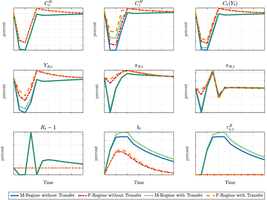
0 2 4 6 8 10 12
-20
-15
-10
-5
0
0 2 4 6 8 10 12
-10
-5
0
0 2 4 6 8 10 12
-15
-10
-5
0
0 2 4 6 8 10 12
-15
-10
-5
0
0 2 4 6 8 10 12
-6
-4
-2
0
0 2 4 6 8 10 12
-15
-10
-5
0
5
10
0 2 4 6 8 10 12
0
0.01
0.02
0.03
0.04
0 2 4 6 8 10 12
0
10
20
30
0 2 4 6 8 10 12
0
5
10
15
20
Appendix Figure B.3: Redistribution Policy with Different Policy Regimes (ε = 1.2)
Notes: This figure shows dynamics of key variables in response to the COVID shocks under different
regimes when ε = 1.2. Blue solid lines represent the baseline case: the monetary regime without trans-
fers. Red dashed lines, green dotted lines, and orange dashed lines represent respectively the fiscal
regime without transfers, the monetary regime with transfers, and the fiscal regime with transfers.
45
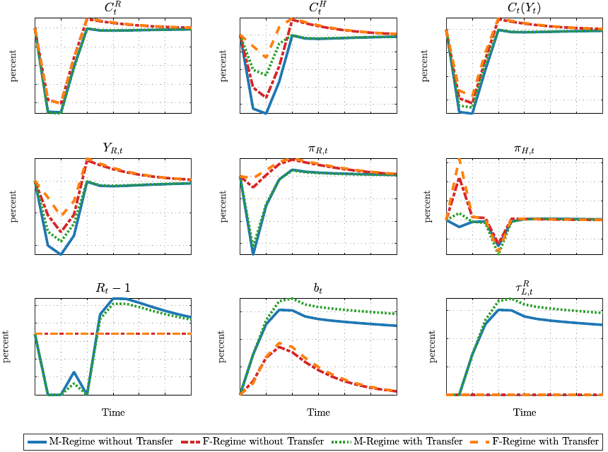
0 2 4 6 8 10 12
-20
-15
-10
-5
0
0 2 4 6 8 10 12
-8
-6
-4
-2
0
0 2 4 6 8 10 12
-15
-10
-5
0
0 2 4 6 8 10 12
-10
-5
0
0 2 4 6 8 10 12
-6
-4
-2
0
0 2 4 6 8 10 12
-5
0
5
10
15
0 2 4 6 8 10 12
0
0.002
0.004
0.006
0.008
0.01
0 2 4 6 8 10 12
0
10
20
30
0 2 4 6 8 10 12
0
1
2
3
Appendix Figure B.4: Redistribution Policy with Different Policy Regimes (ψ
L
= 0.1)
Notes: This figure shows dynamics of key variables in response to the COVID shocks under different
regimes when ψ
L
= 0.1. Blue solid lines represent the baseline case: the monetary regime without
transfers. Red dashed lines, green dotted lines, and orange dashed lines represent respectively the fiscal
regime without transfers, the monetary regime with transfers, and the fiscal regime with transfers.
46
