
Exit Strategies from Quantitative Easing:
The role of the fiscal-monetary policy mix
∗
Florencia S. Airaudo
†
January 15, 2023
Please download here the most recent version of this paper
Abstract
As a consequence of the policy responses to the COVID-19 crisis, central bank bal-
ance sheets, public debt, and liquidity increased in many developed economies. As the
economies recover and inflation far exceeds the target, central banks face a challenge
in how to manage their balance sheet. I study the macroeconomic effects of reducing
the central bank balance sheet size, i.e., Quantitative Tightening (QT). I construct a
Regime-Switching New Keynesian DSGE model calibrated to the US economy. The
economy fluctuates between a monetary-led regime, a fiscally-led regime, and the zero
lower bound on the monetary policy interest rate. The macroeconomic effects of QT
crucially depend on the fiscal-monetary policy mix. In a monetary-led regime, QT
effectively reduces inflation at the cost of increasing the government debt-to-GDP ra-
tio. In contrast, unwinding the central bank balance sheet in a fiscally-led regime has
little impact on inflation. The negative demand effect driven by QT is not enough to
counteract the stimulative impact of negative real interest rates and fiscal stimulus.
Keywords: Monetary Policy; Fiscal and monetary policy mix; Quantitative Easing;
Quantitative Tightening
JEL Classification: E31, E52, E58, E62, E63
∗
I am indebted to Hernán Seoane for his invaluable support and guidance and to Evi Pappa and Ulf
Söderström for insightful discussions. For helpful comments and suggestions, I am grateful to Carlo Galli,
Andrew Foerster, David Vestin, Roberto Billi, Anna Rogantini Picco, the Economics department of Univer-
sidad Carlos III, especially the participants of the Macroeconomics Reading group, and the Macro Work in
Progress. I thank the members of the Research Division at the Riksbank and the participants of the First
Ph.D. Workshop in Money and Finance at the Riksbank, the Doctoral Workshop on Quantitative Dynamic
Economics at the University of Konstanz, the Annual Meeting of the AAEP, Simposio de la Asociacion
Española de Economia 2022, members of the RedNIE, and participants of the ENTER Seminar at the Uni-
versity College London. I thank financial support by PID2019-107161GB-C31/AEI/10.13039/501100011033
and Ministerio de Asuntos Económicos y Transformación Digital through grant Number ECO2016-76818-C3-
1-P, and to Álvaro Escribano Sáez for his financial support through the Ministerio de Ciencia e Innovación
(Spain), grant RTI2018-101371-B-I00.
†
Department of Economics, Universidad Carlos III de Madrid, Calle Madrid 126, 28903 Getafe, Madrid,
1

“...I would just stress how uncertain the effect is of shrinking the balance sheet..."
J. Powell, Federal Reserve Chairman, press conference May 2022.
1 Introduction
In the Great Recession and the COVID-19 crisis, short-term interest rates in the US ap-
proached the zero lower bound (ZLB), leaving the Federal Reserve without its conventional
monetary policy instrument. Due to this, the Federal Reserve began applying unconven-
tional monetary policies, such as Quantitative Easing (QE), to stimulate the economy by
lowering long-term interest rates.
1
QE consists of expanding the central bank balance sheet
by purchasing large amounts of assets and paying by issuing reserves.
2
At the same time,
the government embarked on a fiscal expansion that increased debt-to-GDP ratios to levels
not seen since World War II.
As the economy recovers and inflation reaches levels not seen in forty years, the Federal
Reserve faces the challenge of how to combine its two main policy tools (short-term interest
rate and balance sheet size) to stabilize the inflation rate. In this paper, I quantify the impact
of reducing the central bank balance sheet size on macroeconomic and financial variables such
as inflation, public debt, and yield spreads. To this end, I construct a Regime-Switching
New Keynesian Dynamic Stochastic General Equilibrium (NK-DSGE) model where fiscal
and monetary authorities are subject to regime changes in their policy rules.
The main contribution of this paper is to show that the macroeconomic impact of QT
depends on how the public debt will be stabilized, i.e., through fiscal surpluses or inflation.
When the fiscal authority adjusts taxes to stabilize the debt, QT reduces inflation, even
under smaller increases in the short-term interest rate. However, shrinkage of the central
bank balance sheet has little impact on inflation if there is no appropriate fiscal framework
to stabilize government debt.
1
Other central banks in developed economies, like the Bank of England, the central bank of Sweden, and
the ECB, among others, implemented similar policies.
2
In practice, QE includes distinct policies. In this paper, QE consists of central bank purchases of
long-term public bonds by selling short-term assets (bank reserves). The main objective of this policy is
to stimulate output and inflation by lowering long-term yields. This policy was defined as QE-type 2 by
Ricardo Reis in his talk “The original sin of QE."
2

The distinctive features of my model rely on the design of the financial intermediaries
and the fiscal and monetary authorities. The model exhibits market segmentation in the
public debt market and a leverage constraint for financial intermediaries, as in Elenev et al.
(2021). The fiscal authority issues long and short-term bonds, while the central bank issues
reserves. The central bank does conventional monetary policy, which consists in setting the
short-term interest rate, and unconventional monetary policy, which consists of central bank
purchases of long-term government bonds, paid by issuing reserves.
QE operates through two channels in this model. First, bank reserves and deposits
increase when the central bank expands its balance sheet. Second, the long-term yield falls
due to the central bank’s intervention in the long-term bond market. This yield decline
gives households incentives to rebalance their portfolio, selling long-term bonds in exchange
for deposits. QE transmits into the economy as a positive demand shock. The portfolio
revaluation effect provides households with a wealth effect, increasing consumption demand.
The fall in savings return generates a substitution effect from savings to consumption. Both
channels operate by increasing aggregate demand. The extent to which QE increases output
and inflation depends on the fiscal-monetary policy mix.
Conventional monetary and fiscal policies consist of a Taylor rule for the short-term
interest rate (the return on short-term public bonds and reserves) and a fiscal rule for taxes.
These rules switch between three policy regimes, as in Bianchi and Melosi (2017) and Bianchi
and Melosi (2022): a monetary-led regime, a fiscal-led regime, and the ZLB regime. In the
first regime, the central bank reacts strongly to inflation deviations from the target, and the
fiscal authority adjusts the primary fiscal surplus to stabilize the public debt.
3
The opposite
happens in the second regime, where the fiscal authority does not adjust the fiscal surplus
enough to stabilize the debt. As a result, the monetary authority allows the inflation rate to
deviate from the target to stabilize debt in real terms. Finally, the ZLB regime represents a
crisis regime, where the monetary authority is constrained by the effective lower bound.
3
This behaviour was characterized as active monetary policy and passive fiscal policy in Leeper (1991)
and the following literature. The opposite happens in the fiscally-led regime, where monetary policy is
passive and fiscal policy active. The literature has also called the regimes monetary dominance and fiscal
dominance, respectively. These regimes represent, in a parsimonious way, the outcome of a game between
fiscal and monetary authorities.
3
The economy presents recurrent regime switches following a transition matrix. Differently
from Bianchi and Melosi (2017) and Bianchi and Melosi (2022), the transition to and from
the ZLB regime is endogenous and depends on macroeconomic conditions. This endogeneity
allows agents to form rational expectations regarding the occurrence of this regime based on
their knowledge of macroeconomic variables such as inflation, output, and nominal interest
rates. The endogenization of this transition probability constitutes one of the contributions
of this paper.
I calibrate the model for the US economy and show it can match volatility and cyclicality
features in the data. Thus, I use it as a laboratory to study central bank balance sheet
policies. I simulate a crisis that resembles the COVID-19 pandemic and the policy response.
I show that a QE program that increases central bank long term bonds purchases by 10p.p.
of GDP reduces the severity of the crisis. Output growth falls around 1p.p. less than without
the program and recovers much faster, allowing a shorter duration of the ZLB regime. QE
also has expansionary effects in terms of inflation. Prices fall by 2.5p.p. less than without
the central bank’s intervention, at the cost of more significant inflationary dynamics during
the recovery, where annualized inflation reaches a peak of 8.1. Without QE, inflation would
have still overshot the target, but with a lower peak of 6.6%.
I show that how the central bank balance sheet’s size is reduced matters for inflation,
output, and debt dynamics. In the crisis recovery, I study different strategies regarding
the size of the central bank balance sheet: 1) maintaining the enlarged size after the crisis
(tapering), 2) decreasing the balance sheet size: a) by letting the bonds that mature, run off
the balance sheet (Quantitative Tightening (QT)), and b) at a faster speed by selling bonds
(Aggressive QT ).
When the central bank reduces its purchases of long-term public bonds, it triggers a fall
in their price and an increase in long-term yields. Increased returns result in a substitution
effect from consumption to savings, reducing aggregate demand and output. At the same
time, public debt issuance increases for three reasons. First, the increase in interest rates
increases debt service. The fall in output triggers automatic stabilizers that increase the
fiscal deficit. The fall in long-term bonds price reduces central bank remittances to the
treasury.
4

In the monetary-led regime, the increase in debt causes a rise in taxes due to the fiscal
rule. This exacerbates the fall in aggregate demand and disinflationary effects of Quantitative
Tightening. In this regime, inflation falls even with lower increases in the policy rate. In the
fiscally-led regime, public debt increases actual and expected inflation, exacerbating the rise
in yield spreads and mitigating the disinflationary effects of QT.
In a fiscally-led regime, thus, there are no clear advantages in reducing the balance sheet
size since it increases debt and spreads without helping to stabilize inflation. The negative
demand shock generated by QT is not enough to counteract the stimulative effect of real
negative interest rates and fiscal deficits.
Related Literature. This paper contributes to several strands of the literature. In
particular, it contributes to the literature that studies the real and inflationary effects of
QE through different channels.
4
Many authors studied the transmission mechanisms of QE
in general equilibrium models, either with financial frictions, like in Gertler and Karadi
(2011), Sims and Wu (2021), Sims et al. (2020), Del Negro et al. (2017), among others; with
market segmentation or portfolio adjustment costs as the main mechanisms to break the
non-arbitrage condition between short-term and long-term bonds, as in Chen et al. (2012),
Harrison (2017), or information frictions as in Gaballo and Galli (2022). Furthermore, a
recent paper by Cui and Sterk (2021) studies the liquidity effects of asset purchase programs
in a model with heterogeneous agents. The main contribution to this strand of the literature
is allowing the fiscal-monetary policy mix to play a role in shaping the macroeconomic effects
of QE and showing alternative scenarios where fiscal and monetary policy interact.
In a related paper, Elenev et al. (2021) ask whether monetary policy can create fiscal
capacity. In their setting, fiscal capacity depends on the probability of shifting fiscal policy
from active to passive. In this sense, I share with them the objective of studying the effects
of unconventional monetary policies while allowing fiscal policy to shift between regimes.
The main difference with this paper is that Elenev et al. (2021) assume and estimate a fiscal
limit beyond which the Treasury starts increasing taxes to ensure debt sustainability. At
the same time, the conventional monetary policy is active at all periods. These assumptions
prevent inflationary dynamics from arising in the model since all the agents in the economy
4
See Bhattarai and Neely (Forthcoming) and Kuttner (2018) for reviews of this literature.
5
are rational and know the government will never inflate away part of the debt. My main
contribution here is to study QT when fiscal and monetary authorities can follow a different
policy configuration.
By giving a central role to the interaction or coordination of fiscal and monetary policies,
this paper also relates to the literature that studies fiscal-monetary policy mix, as in Sims
(1994), Leeper (1991), Schmitt-Grohe et al. (2007), Leeper and Leith (2016), Reis (2017),
Bassetto and Sargent (2020), Barthélemy et al. (2021), among others, and to the literature
of the Fiscal Theory of the Price Level as in Sargent et al. (1981), Bassetto (2002), Cochrane
(2001), Sims (2016), Cochrane (2021), Brunnermeier et al. (2020). Allowing the policy mix
to alternate, this paper also relates to the literature on regime switches in policy rules, as in
Bianchi (2013), Bianchi and Melosi (2017), Bianchi and Melosi (2022), among others. The
contribution to this branch of the literature is the study of unconventional monetary policies
together with the conventional Taylor rule on short-term interest rates. By considering an
endogenous transition probability to get in and out of the ZLB, this paper relates to the
literature that studies monetary policy rules that depend on endogenous variables, as in
Barthélemy and Marx (2017), Davig and Leeper (2008).
This paper focuses on the macroeconomic effects of reducing the central bank balance
sheet. In a broad sense, I share the question with, for example, Wen et al. (2014), Harrison
(2017), Sims et al. (2020), Bonciani and Oh (2021), Hall and Reis (2016), Foerster (2015)
and Benigno and Benigno (2022). However, this paper differs from these in many aspects.
In Wen et al. (2014), the focus relies on the impact on firms, while there is no role for the
fiscal authority. Harrison (2017) studies the optimal QE policy in a DSGE-NK model with
portfolio adjustment costs, and Sims et al. (2020) studies optimal simple and implementable
QE rules through minimizing a quadratic loss-function in a DSGE-NK model with financial
frictions. Bonciani and Oh (2021) extends the work of Sims et al. (2020) by showing that
the central bank’s loss function depends on its asset purchase volatility. Crucial differences
are that these articles focus on central bank purchases of corporate/ private sector bonds,
assume a limited role in fiscal policy, and do not allow for changes in the conduct of the fiscal
policy rule. Hall and Reis (2016) study how different strategies for the exit from quantitative
easing in the face of interest-rate risk, as I do. However, the authors’ main objective is to
6
study the implications on central bank financial stability, and they assume a passive fiscal
policy. Foerster (2015) examines the macroeconomic effects of unwinding the central bank
balance sheet during and after a financial crisis. He shows that private agents’ expectations
about the exit strategy from a QE program impact the initial effectiveness of the policy in
a MS-DSGE model with a financial sector. However, there is no role for parameter switches
in conventional policy rules, abstracting from the possibility of alternative fiscal-monetary
policy interactions, which is the main contribution of this paper.
Finally, in a recent related paper, Benigno and Benigno (2022) study monetary policy
normalization, defined as the combination of lifting the policy rate and reducing the size of
central bank balance sheets. They study how these monetary policies interact and how they
depend on the behavior of the fiscal authority. However, they focus on optimal policy analysis
and does not account for policy uncertainty in the configuration of fiscal and monetary policy
interactions, which constitutes a central contribution of this paper.
The remainder of the paper is as follows. In the following section, I provide motivating
evidence of the importance of the fiscal and monetary policies interaction during Quantitative
Easing programs, looking at data for the US during the COVID-19 crisis. Section 3 presents
the model, Section 4 discusses the calibration, functional forms, and solution method. In
Section 5, I present the quantitative results of the model, and in Section 6 explain the main
transmission mechanism of QE. Section 7 presents the paper’s main results, where I simulate
the crisis and present the different exit strategies from QE. Finally, Section 8 concludes.
2 COVID-19 crisis and policy response in the US
This section provides data on the COVID-19 crisis and the policy response in the US. The
objective is to show the behavior of the main players in the bonds market, which motivates
some model decisions.
In March 2020, the COVID-19 pandemic hit economies worldwide, generating an unprece-
dented macroeconomic crisis. As a response, central banks in leading developed economies,
particularly the US, started to stimulate the economy through cuts in short-term interest
rates until they hit the zero lower bound. As a result, central banks began Quantitative
7
Easing programs. They consisted of purchasing assets, mainly government bonds of long
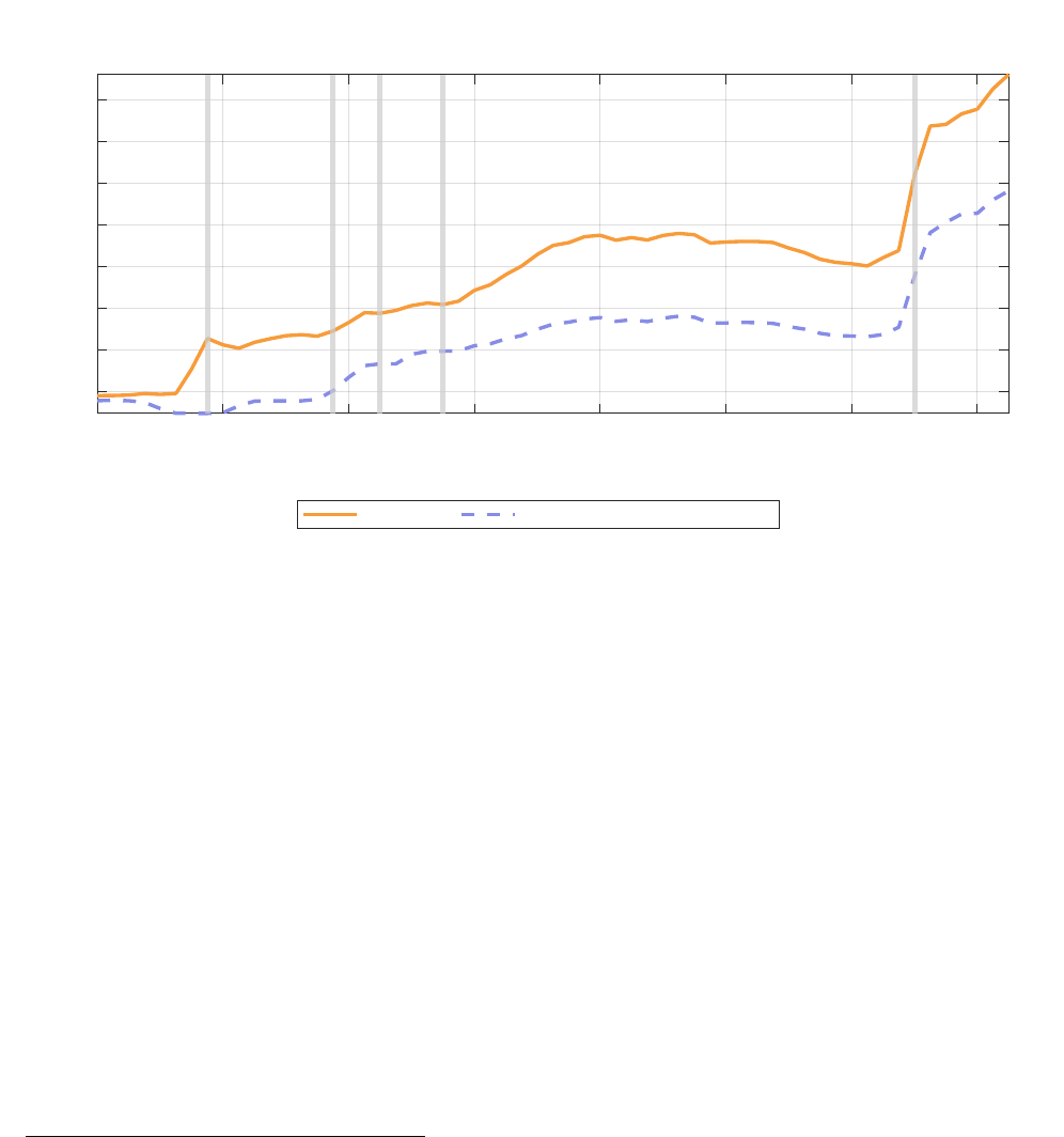
maturity, expanding their balance sheets at a breakneck speed. As shown in figure 1, the
assets in the Federal Reserve increased from $4 trillion in the third quarter of 2019 to over
$8 trillion one year later. Treasuries are the main component of this assets’ expansion at the
Federal Reserve, which increased from about $2 to $6 trillion in less than two years.
2007Q1 2009Q1 2011Q1 2013Q1 2015Q1 2017Q1 2019Q1 2021Q1
1
2
3
4
5
6
7
8
Trillions USD
Fed Assets Treasuries in Fed balance sheet
Figure 1: Federal Reserve Balance Sheet
Assets in the Federal Reserve balance sheet (orange line) and treasuries in the balance sheet
(dotted light-blue line). Variables in trillions of dollars. Source: FRED and US Financial
Accounts. Grey vertical lines show the start of a Quantitative Easing program.
The Quantitative Easing program took place with a substantial expansion in total debt
issuance from the Treasury. Figure 2 shows net purchases of treasuries from the start of the
COVID-19 crisis. They are net flows of treasuries, i.e., net of revaluation effects that take
into account the change in treasuries’ prices.
5
Different colors represent different agents in
the economy. When the bar is above zero, the agent had net purchases of treasuries during
the period, while if it is below zero, it represents net sales. The blue line represents the net
5
The conclusions do not change when we consider changes in treasuries. See Appendix, section 9.1.
8
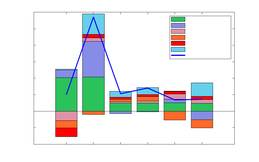
debt issuance from the US Treasury, which is the sum of all the bars in a corresponding
period.
The figure shows the significant increment in debt issuance during the whole period.
Furthermore, the monetary authority’s purchases of government bonds played a vital role
during this period, sustaining the demand for treasuries when private sectors like households,
mutual funds, and the rest of the world were selling their bond holdings.
2020Q1 2020Q2 2020Q3 2020Q4 2021Q1 2021Q2
-1000
-500
0
500
1000
1500
2000
2500
3000
Monetary Authority
Money Market Funds
Rest of the world
Household sector
Mutual funds
Others
Net debt issuance
Figure 2: Net purchases of treasuries
Source: US Financial Accounts. Data in billions of dollars. Flows, net of revaluation effects.
Who sells treasuries to the central bank during a QE operation has implications regarding
the primary macroeconomic aggregates in the economy. When the Federal Reserve performs
quantitative easing policies, it purchases assets. The counterpart of this operation is the
issuance of bank reserves (or money in commercial banks’ hands) that increases the central
bank’s liabilities, expanding the central bank’s balance sheet. If commercial banks were the
original owners of the bonds (case 1), this operation would leave its balance sheet unchanged
since they increase one asset (reserves) while decreasing another (treasuries). However, sup-
pose the original owner of the bond was the non-bank private sector (case 2), like households
9
or mutual funds. In that case, the bank is a intermediary of this policy. The result would
be an increase in deposits or currency (money in private hands), together with an increase
in reserves and the central bank’s balance sheet. As a result, different measures of money
increase after quantitative easing policies under different cases; either bank money in the
form of reserves (case 1) or non-bank private money (case 2).
2019Q4
2020Q1
2020Q2
2020Q3
2020Q4
2021Q1
2021Q2
2021Q3
3
3.5
4
4.5
5
5.5
Debt purchases by FED
2019Q4
2020Q1
2020Q2
2020Q3
2020Q4
2021Q1
2021Q2
2021Q3
2
2.5
3
3.5
Reserves
2019Q4
2020Q1
2020Q2
2020Q3
2020Q4
2021Q1
2021Q2
2021Q3
14
15
16
17
Comercial banks deposits
2019Q4
2020Q1
2020Q2
2020Q3
2020Q4
2021Q1
2021Q2
2021Q3
1.5
2
2.5
3
3.5
4
Core Inflation (yoy)
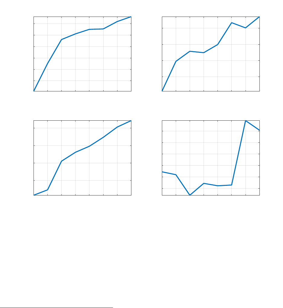
Figure 3: Macroeconomic variables: public debt, liquidity, inflation
US Federal Debt, Reserves and Deposits, in trillions of dollars. Core inflation in %. Source
debt, deposits, and inflation data: FRED. Source reserves: US financial accounts, released
December 2021.
In figure 3, we can see a great expansion in liquidity, both in the form of bank reserves
and deposits.
6
Other measures of monetary aggregates present significant increases during
6
In the appendix, section 9.1, I show this last feature differs from what happened after the Quantitative
Easing programs after the Great Recession.
10

this period too. Some of these variables, like public debt, are at values over GDP not seen
since the Second World War.
7
As economies recover and face inflationary dynamics not seen in the last 40 years, it is
unclear how to unwind the stimulus injected during the crisis. The combination of high infla-
tion rates, large debt-to-GDP ratios, elevated liquidity, and expanded central bank balance
sheet presents an extra challenge for policymakers.
In the following section, I present a model able to generate the comovements that we ob-
served in aggregate macroeconomic variables during the COVID-19 crisis and the consequent
policy response and use it as a laboratory to study balance sheet policies.
3 Model
The model is a NK-DSGE model with five agents: Firms, households, Monetary Authority,
Fiscal Authority, and financial intermediaries (FI). There are three assets in the economy:
Short-term public bonds B
S
t
with one-period maturity and price Q
S
t
; deposits D
t
which
provide liquidity services to households and with price Q
D
t
; and long-term public bonds: B
L
t
,
with geometrically decaying maturity δ, as in Hatchondo and Martinez (2009), that pay a
coupon κ every period, and their price is Q
L
t
.
As is standard in the literature that assesses the transmission mechanisms of quantitative
easing policies, there is segmentation in bond markets.
8
I follow Elenev et al. (2021) in as-
suming that households cannot invest in short-term public bonds, which are held exclusively
by financial intermediaries and the central bank. In contrast, financial intermediaries do
not invest in long-term public bonds. These assumptions align with the data presented in
section 2.
Short-term bonds in the model stand for treasury bills and central bank reserves indis-
tinctly since both assets share liquidity and return properties. The only difference between
them is which governmental institution issues them (i.e., central bank or treasury). The
7
See section 9.1 for a historical plot of this variable.
8
See, for instance, Chen et al. (2012), and Bhattarai and Neely (Forthcoming) for a comprehensive
analysis on different mechanisms to break the non-arbitrage condition between different assets in the economy,
and thus, the neutrality result from Wallace (1981).
11

assumption that financial intermediaries exclusively hold them in the model makes this asset
close to “money in banks’ hands.”
Market segmentation interacts in the model with the following frictions. First, prices are
sticky, as in Rotemberg (1982) and the New-Keynesian literature. Second, households pay
a portfolio adjustment cost when purchasing long-term public bonds, and financial interme-
diaries pay a convex cost when they raise new equity. Finally, financial intermediaries are
subject to a leverage constraint that states that their debt (deposits) cannot be larger than
their assets (reserves and treasury bills). On top of this, the real value of deposits provides
liquidity services to households increasing their utility, as in the tradition of Money in the
Utility (MIU) function models. Including variables that stand for reserves and monetary
aggregates in the model, together with the frictions above, allows the model to generate the
main macroeconomic effects of QE policies highlighted in the empirical literature and the
comovements in macroeconomic aggregates that we observed in section 2.
Two authorities constitute the government: the treasury and the central bank. Each
authority has its budget constraint and policy instrument(s). The presence of the two gov-
ernmental sectors allows the model to generate realistic policy interactions, which are at the
center of macroeconomic dynamics. I follow Bianchi and Melosi (2017), and Bianchi and
Melosi (2022) and assume that parameters in policy rules for conventional monetary policy,
the Taylor rule, and fiscal rule alternate between regimes.
Next, I describe each agent and its optimization problem.
3.1 Households
There is a continuum of measure one of homogeneous households that live infinite periods
in the economy. A representative agent chooses consumption c
t
, labor n
t
, deposits D
H
t
, and
long-term public bonds B
L,H
t
to maximize its lifetime utility:
E
0
∞
X
t=0
ν
t
β
t
U
c
t
,
D
H
t
P
t
, n
t
ν
t
is a preference shock that follows an AR(1) process. Deposits are the most liquid asset
that a household can purchase. I assume agents derive utility from the liquidity services
12

this asset provides. The utility function is a monotone increasing function in consumption
and deposits, a monotone decreasing function in labor, and satisfies Inada conditions on all
variables.
Long-term bonds pay geometrically decaying coupons, as in Hatchondo and Martinez
(2009). A bond B
L
t
issued at time t pays the sequence of coupons: κ, κ(1 − δ), κ(1 − δ)
2
, ...,
where κ > 0 and δ ∈ (0, 1). This last parameter controls the debt maturity, where δ = 1
corresponds to a short-term bond (i.e., 1-period maturity), and δ = 0 represents a consol.
This maturity specification reduces the number of state variables in the model. A bond
issued at time j − k is equivalent to (1 − δ)
k
bonds issued at period t, and hence the state
variable B
L
t−1
represents total long-term debt in equivalent newly issued long-term bonds.
Their price at period t is Q
L
t
.
9
Every period, the representative household pays lump-sum taxes τ
t
, receives nominal
dividend payments from financial intermediaries Div
t
, firm’s profits since households are
the owners Π
f
t
, and rebates
˜
Π
t
. When she invests in long-term bonds, she pays a portfolio
adjustment cost of Φ(.) on top of the asset’s price.
10
The optimization problem of a representative household is the following.
max
c
t
,n
t
,D
H
t
,B
L,H
t
E
0
∞
X
t=0
β
t
ν
t
U
c
t
,
D
H
t
P
t
, n
t
P
t
c
t
+ Q
D
t
D
H
t
+ B
L,H
t
Q
L
t
+ Φ
L
B
L,H
t
P
t
!
P
t
= W
t
n
t
+ D
H
t−1
+ · · ·
+B
L,H
t−1
κ + (1 − δ)Q
L
t
+ Π
f
t
+ Div
t
+
˜
Π
t
− τ
t
P
t
(1)
D
H
t
≥ 0
B
L,H
t
≥ 0
9
Notice that the deflated number of nominal bonds by the price level,
B
L,H
t
P
t
= b
L,H
t
is not the real value
of public debt. Instead, the real value of public bonds held by households is Q
L
t
B
L,H
t
P
t
. As discussed in Leeper
et al. (2021), introducing the variable b
L,H
t
allows to dispose of one variable, by working with b
L,H
t
instead
of P
t
and B
L,H
t
.
10
This assumption helps the model generate a positive term premium in long-term public bonds.
13

where P
t
is the price level, and W
t
is the nominal wage. Under this specification, the expected
return on a long-term bond purchased at period t is R
L
t,t+1
= E
t
κ+(1−δ)Q
L
t+1
Q
L
t
.
Notice that the non-negativity condition on deposits does not bind at the optimum even
if they pay a lower return, given the assumption that deposits increase utility. Finally, the
last constraint is the non-negativity conditions for public bonds since the household cannot
go short on them.
Associate the multiplier β
t
λ
t
to the budget constraint. The system of equilibrium condi-
tions that characterize the households’ optimization problem solution is the following:
−U
n
c
t
,
D
H
t
P
t
, n
t
U
c
c
t
,
D
H
t
P
t
, n
t
=
W
t
P
t
Q
D
t
= E
t
M
t,t+1
+
U
d
c
t
,
D
H
t
P
t
, n
t
P
t
U
c
c
t
,
D
H
t
P
t
, n
t
Q
L
t
+ Φ
′
L
B
L,H
t
P
t
!
= E
t
M
t,t+1
κ + (1 − δ)Q
L
t+1
Where M
t,t+1
is the stochastic discount factor between period t and t + 1.
M
t,t+1
= β
λ
t+1
λ
t
= β
ν
t+1
ν
t
U
c
c
t+1
,
D
H
t+1
P
t+1
, n
t+1
U
c
c
t
,
D
H
t
P
t
, n
t
1
π
t+1
Together with the budget constraint (1), they characterize the solution to the household’s
optimization problem.
11
Define π
t
=
P
t
P
t−1
as the inflation rate of period t. Notice that
a spread will exist between the prices of deposits and long-term bonds even without the
presence of portfolio adjustment cost. Households are willing to invest in deposits, even
though they provide a lower return, because they derive utility from them. The presence
of portfolio adjustment costs in bonds generates a term spread and prevents the household
from fully exploiting the arbitrage opportunities in the assets’ markets. The literature has
shown this feature is vital for the transmission mechanism of QE policies.
11
The non-negativity condition in public bond purchases ensures the transversality condition is satisfied.
14

For future reference, it is convenient to define the return on a risk-free private asset in
this economy, which is in zero net supply, as given by:
R
N
t
= E
t
1
M
t,t+1
This expression is defined as the natural interest rate in Benigno and Benigno (2022),
which differs from the policy rate, and is key in the consumption-savings trade-off.
3.2 Firms
The productive sector comprises two levels: final goods and intermediate goods producers.
3.2.1 Final good producer
A representative firm produces the domestic final good y
t
from varieties y
i
, for i ∈ [0, 1].
y
t
=
Z
1
0
y
ε−1
ε
i,t
di
ε
ε−1
Where ε is the elasticity of substitution between varieties. The optimization problem of the
representative firm is the following:
max
y
t
,{y
i,t
}
i∈[0,1]
P
t
y
t
−
Z
1
0
P
i,t
y
i,t
di
s.t y
t
=
Z
1
0
y
ε−1
ε
i,t
di
ε
ε−1
And the optimal demand function for variety i is given by the following expression:
y
i,t
= y
t
P
i,t
P
t
−ε
(2)
15

3.2.2 Intermediate goods firms
Intermediate goods firms are monopolistically competitive in the goods market. Each firm
produces a variety i according to a linear production function:
y
i,t
= z
t
n
i,t
(3)
Where z
t
is a mean reverting TFP shock, common to all varieties, with the law of motion:
ln (z
t
) = ρ
z
ln (z
t−1
) + σ
z
ε
z
t
, ε
z
t
∼ N(0, 1)
When changing prices, firm i is subject to a quadratic adjustment cost in prices, as in
Rotemberg (1982):
ϕ
P
2
P
i,t
P
i,t−1
− π
∗
2
y
t
Where ϕ
P
measures the degree of nominal price rigidity, and y
t
is aggregate output, given
by:
y
t
=
Z
1
0
y
i,t
di
The nominal profit of firm i at period t, transferred to households, is given by:
Π
f
i,t
= P
i,t
y
i,t
− W
t
n
i,t
−
ϕ
P
2
P
i,t
P
i,t−1
− π
∗
2
y
t
P
t
(4)
Firms maximize the discounted sum of profits using the households’ discount factor, and
subject to technology 3, and demand 2.
16

Their optimization problem is the following:
max
P
i,t
,n
i,t
E
0
∞
X
k=0
M
t,t+k
Π
f
i,t+k
s.t. y
i,t
= z
t
n
i,t
y
i,t
= y
t
P
i,t
P
t
−ε
Π
f
i,t
= P
i,t
y
i,t
− W
t
n
i,t
−
ϕ
P
2
P
i,t
P
i,t−1
− π
∗
2
P
t
y
t
In equilibrium, all firms behave symmetrically, and we have P
i,t
= P
t
. Thus, aggregate
profits are given by:
Π
f
t
= P
t
y
t
− W
t
n
t
−
ϕ
P
2
(π
t
− π
∗
)
2
y
t
P
t
Their optimization problem is characterized by the following conditions, where MC
t
is
the multiplier of equation 2, and it is the marginal cost.
1 − ε + ε
MC
t
P
t
= ϕ
P
(π
t
− π
∗
) π
t
− ϕ
P
E
t
M
t,t+1
y
t+1
y
t
π
2
t+1
(π
t+1
− π
∗
)
(5)
W
t
= MC
t
z
t
(6)
The first condition is the New-Keynesian Phillips curve.
3.3 Financial intermediaries
In this section, I follow a simplified version of the financial intermediaries’ description in
Elenev et al. (2021).
A representative agent in this sector starts the period t with a net worth of W
I
t
. Every
period, it pays a fraction τ
I
of its net worth to households and raises new equity from them,
A
t
. The net payout to shareholders is then:
Div
t
= τ
I
W
I
t
− A
t
(7)
17

This agent can invest in short-term public bonds B
S,I
t
for the price Q
S
t
. B
S,I
t
is the
sum of treasury bills (treasuries with a maturity of up to a year, B
S
t
) and central bank
reserves (B
S,CB
t
). The reason for adding these assets into one variable is that they have the
same risk and return properties in the model, being perfect substitutes from the financial
intermediaries’ point of view. Its liabilities are given by deposits from households D
I
t
. The
following expression then gives the balance sheet:
(1 − τ
I
)W
I
t
+ A
t
− Φ
A
(A
t
) + Q
D
t
D
I
t
= Q
S
t
B
S,I
t
(8)
Where Φ
A
(.) is a convex cost of issuing new equity, rebated lump-sum to Households. This
cost prevents financial intermediaries from raising funds only through equity, going to a
corner solution with D
I
t
= 0.
The net wealth at period t is:
W
I
t
= B
S,I
t−1
− D
I
t−1
(9)
In line with Basel regulation, financial intermediaries are subject to a leverage constraint.
It states that their debt (in this case, deposits) can be, at most, a fraction ζ of its assets.
12
D
I
t
≤ ζB
S,I
t
(10)
The optimization problem of a financial intermediary consists of maximizing the dis-
counted sum of dividends subject to restrictions 8, 9, and 10. I assume the financial inter-
mediary discounts its future flows using the household’s stochastic discount factor.
12
I assume the financial intermediary sector’s assets are composed only of treasury bills and central bank
reserves for simplicity. In a more complicated model, they could also purchase firms’ bonds or provide loans
to firms to finance capital purchases. This is the case in Elenev et al. (2021), and Benigno and Benigno
(2021). The qualitative conclusions of this paper do not change when considering a more complicated version
of the model, reducing to quantitative differences.
18

max
A
t
,D
I
t
,B
S,I
t
E
0
∞
X
k=0
M
t,t+k
τ
I
W
I
t+k
− A
t+k
s.t. (1 − τ
I
)W
I
t
+ A
t
− Φ
A
(A
t
) + Q
D
t
D
I
t
= Q
S
t
B
S,I
t
W
I
t
= B
S,I
t−1
− D
I
t−1
D
I
t
≤ ζB
S,I
t
Define η
t
as the Balance sheet multiplier and µ
t
as the Leverage constraint multiplier.
Using the first order condition to equity A
t
to substitute out the multiplier η
t
, we obtain
the system of equations that characterize the financial intermediary’s optimization problem,
together with 7, 8, 9, 10:
13
Q
D
t
= E
t
˜
M
t,t+1
+ µ
t
(1 − Φ
′
A
(A
t
)) (11)
Q
S
t
= E
t
˜
M
t,t+1
+ ζµ
t
(1 − Φ
′
A
(A
t
)) (12)
Where
˜
M
t,t+1
is the stochastic discount factor for financial intermediaries, defined as:
˜
M
t,t+1
≡ M
t,t+1
(1 − Φ
′
A
(A
t
))
τ
I
+
1 − τ
I
1 − Φ
′
A
(A
t+1
)
Notice that the spread between deposits and short-term bonds is a function of the leverage
constraint multiplier µ
t
. Since ζ < 1, the return on short-term bonds is higher than the
short-term bonds when the leverage constraint binds. If the leverage constraint does not
bind, then we get Q
S
t
= Q
D
t
, and from the Households’ problem, this could only be possible
in a situation where liquidity services are zero.
3.4 Monetary Authority
The Central Bank performs conventional and unconventional monetary policies. The con-
ventional monetary policy sets the short-term nominal interest rate R
t
, subject to a ZLB
13
See appendix, section 9.2 for further details.
19

restriction. This rate is the inverse of the short-term public debt price:
R
t
≡
1
Q
S
t
(13)
The unconventional monetary policy consists of central bank balance sheet policies. In
particular, the central bank purchases long-term government debt B
L,CB
t
in exchange for
reserves (B
S,CB
t
), as in the data since the Great Recession. The rules for setting these two
instruments are provided in a following section.
The following expression gives the Central Bank’s budget constraint:
B
S,CB
t−1
P
t
+
B
L,CB
t−1
P
t
κ + (1 − δ)Q
L
t
= Q
S
t
B
S,CB
t
P
t
+ Q
L
t
B
L,CB
t
P
t
+ Λ
CB
t
where Λ
CB
t
are central bank remittances to the fiscal authority. I assume that profits Λ
CB
t
are transferred to the fiscal authority.
14
Finally, the central bank is subject to a revenue neutrality constraint, which is in line with
the data. It states that when the central bank increases its assets by purchasing long-term
bonds, it has to offset the operation by decreasing its net position of short-term assets.
Q
L
t
B
L,CB
t
+ Q
S
t
B
S,CB
t
= 0 (14)
When it performs QE, we have B
S,CB
t
< 0, representing the increase in reserves issuance.
3.5 Fiscal Authority
The treasury consumes g
t
and obtains resources from three different sources. It collects tax
revenues from households in a lump-sun fashion, τ
t
, receives dividends from the central bank
Λ
CB
t
, and issues debt, whose total real value is
B
t
P
t
. This debt comprises short-term bonds
14
For simplicity, in this paper, I abstract from asymmetries in the transfer of the central bank’s profits to
the treasury, like the ones discussed in Hall and Reis (2016).
20

B
S
t
and long-term bonds B
L
t
. The total debt issuance is:
15
B
t
= Q
S
t
B
S
t
+ Q
L
t
B
L
t
(15)
The period budget constraint of the fiscal authority, in real terms, is:
τ
t
− g
t
| {z }
≡s
t
+
B
t
P
t
+ Λ
CB
t
=
B
S
t−1
P
t
+
B
L
t−1
P
t
κ + (1 − δ)Q
L
t
Where s
t
is the real primary fiscal surplus of period t. Replacing Λ
CB
t
from the central
bank balance sheet and using 14, I obtain a consolidated budget constraint:
s
t
+
B
t
P
t
=
B
S
t−1
− B
S,CB
t−1
P
t
| {z }
A
+
B
L
t−1
− B
L,CB
t−1
P
t
| {z }
B
κ + (1 − δ)Q
L
t
(16)
The terms’ A’ and ‘B’ are the outstanding short and long-term public debt in the private’s
hands. Notice that through the purchases of long-term public bonds, the central bank relaxes
the budget constraint for the consolidated government. However, this is not necessarily
the case when considering the net position of short-term assets. For instance, if B
S,CB
t
<
0, implying reserves issuance, then the consolidated government debt of short maturity is
increasing with this policy. In this sense, quantitative easing policies can be interpreted as
a maturity swap, exposing the government to interest rate risk.
The following expression gives government consumption:
g
t
= θ(y
∗
− y
t
) + (1 − ρ
g
)¯g + ρ
g
g
t−1
+ σ
g
ε
g
t
, ε
g
t
∼ N(0, 1)
0 < θ < 1 represents the government spending reaction to output deviations from its
steady state. This term generates a counter-cyclical behavior of government consumption,
introducing fiscal stimulus when the economy is in a recession. Government consumption
goods are thrown into the ocean. Finally, the maturity composition of newly issued govern-
ment debt is constant in book value terms, with a fraction ¯µ of debt being long-term.
15
Notice that the real amount of short-term bonds is Q
S
t
B
S
t
P
t
and the one of long-term bonds is Q
L
t
B
L
t
P
t
.
21

B
S
t
B
L
t
=
1 − ¯µ
¯µ
(17)
3.6 Market clearing conditions
Market clearing conditions are the following:
c
t
+ g
t
+
ϕ
P
2
(π
t
− π
∗
)
2
y
t
= y
t
D
H
t
= D
I
t
B
S
t
− B
S,CB
t
= B
S,I
t
B
L
t
= B
L,H
t
+ B
L,CB
t
And households’ rebates by other agents in the model are equal to:
˜
Π
t
= Φ
L
b
L,H
t
+ Φ
A
(A
t
)
3.7 Policy rules
To close the model, I assume that fiscal and monetary authorities follow policy rules to set
their instruments: τ
t
, R
t
, and b
L,CB
t
. First, I assume that central bank purchases of long-term
bonds follow an AR(1) process:
b
L,CB
t
= (1 − ρ
QE
)b
L,CB
∗
+ ρ
QE
b
L,CB
t−1
+ σ
QE
ϵ
QE
t
(18)
Where b
L,CB
∗
is the average amount of long-term bonds at the steady state. Increases in
the central bank balance sheet are random and unrelated to the economic conditions. I follow
this assumption for two reasons. First, this paper aims to study the effects of QE policies
under different interactions of conventional fiscal and monetary policies. Second, there is
no evidence or consensus of a clear rule for central bank purchases, a policy with a great
discretionary component. This assumption implies that QE constitutes a complementary
policy instrument of the central bank and not necessarily a substitute, in line with what we
22

observe in the data. Furthermore, it prevents the instrument from altering the determinacy
properties of the model.
I follow the literature on fiscal-monetary policy interactions and assume that fiscal and
monetary authorities follow rules to determine the conventional policy instruments. In par-
ticular, the nominal short-term interest rate follows the Taylor rule 20, reacting to output
and inflation deviations from its steady state values, together with an autoregressive pa-
rameter ρ
R
and a monetary shock ϵ
m
t
with standard deviation σ
m
t
. The monetary shock
stands for interest rate deviations from the reaction function. The intensity of interest rate
reaction to output and inflation deviations are characterized by policy parameters α
y
and
α
π
, respectively. Finally,
¯
R is the mean of the nominal interest rate.
For fiscal policy, I assume that taxes τ
t
react to total real debt deviations from its steady
state value b
∗
and have an autoregressive coefficient ρ
τ
, as in 19. The elasticity of tax
deviations to debt deviations is characterized by the parameter γ.
16
τ
t
− τ
∗
= ρ
τ
(ξ
t
) (τ
t−1
− τ
∗
) + (1 − ρ
τ
(ξ
t
)) γ (ξ
t
) (b
t−1
− b
∗
) (19)
R
t
¯
R (ξ
t
)
=
R
t−1
¯
R (ξ
t
)
α
R
(ξ
t
)
"
π
t
π
∗
α
π
(ξ
t
)
y
t
y
∗
α
y
(ξ
t
)
#
1−α
R
(ξ
t
)
e
σ
M
(ξ
t
)ϵ
M
t
(20)
The parameters above depend on a discrete shock ξ
t
that follows a Markov process. I fol-
low Bianchi and Melosi (2017) and assume that this shock can take three values, representing
the three regimes through which the economy fluctuates.
The first regime, the monetary-led (M) regime, is characterized by a strong interest rate
reaction to inflation deviations (high α
π
) and a strong tax reaction to debt (high enough
γ).
17
This regime is associated to an active monetary policy and passive fiscal policy, in
Leeper (1991) terminology. Under this regime, the monetary authority adjusts the nominal
16
Assuming the fiscal rule reacts to real public debt in private hands, i.e., Q
L
t
b
L,H
t
+ Q
S
t
b
S,I
t
does not
change the conclusions in this paper. These results are available under request.
17
In Appendix, I present, for a given calibration, the combinations of values α
π
and γ that give rise
to determinacy at each regime. Notice, however, that the global stability of the system does not require
determinacy at each regime.
23
interest rate more than proportionally to changes in the inflation rate to stabilize inflation.
At the same time, the treasury passively adjusts taxes to stabilize the real debt.
The second regime is the fiscally-led regime (F) where the fiscal authority does not adjust
taxes enough to stabilize the real debt (low γ). Then, the central bank allows the inflation
rate to deviate from the target to stabilize debt in real terms. This regime can be defined
as passive monetary policy and active fiscal policy in the sense of Leeper (1991).
The third regime is the Zero Lower Bound regime (ZLB). It is characterized by an un-
reactive nominal short-term interest rate that remains fixed at its effective lower bound and
by a fiscal policy that is unreactive to the real debt level. This regime is an extreme form
of the fiscally led regime since we have α
π
= γ = 0. As in Bianchi and Melosi (2017), this
regime represents a crisis regime, where the economy enters due to the realization of bad
shocks that drive the economy to a recession. However, differently from Bianchi and Melosi
(2017), the economy enters the ZLB regime endogenously, as I explain in the next section.
3.8 Transition probabilities
Assume the Markov-switching shock ξ
t
depends on the realization of two random variables
ξ
P
t
and ξ
C
t
. When ξ
C
t
= 1, the economy suffers a crisis and moves to the ZLB regime. When
ξ
C
t
= 0, the government can set fiscal and monetary policies without restriction. In this
case, the variable ξ
P
t
determines the regime in place stochastically. ξ
P
t
= M stands for the
monetary-led regime, ξ
P
t
= F for the fiscally-led regime, and it evolves according to the
transition matrix:
P =
p
mm
1 − p
mm
1 − p
ff
p
ff
where p
ij
= P
ξ
P
t+1
= j|ξ
P
t
= i
.
As seen from the transition matrix P, the probability of being in one regime or another
is constant and entirely exogenous. The realization of this shock represents, in a simplified
way, the outcome of a policy game between the fiscal and the monetary authority, where the
winner is the active authority.
24

Define q as the probability of entering to the ZLB regime, q = P (ξ
C
t+1
= 1|ξ
C
t
= 0) and r
as the probability of moving out of the crisis regime q = P (ξ
C
t+1
= 0|ξ
C
t
= 1).
The transition matrix for ξ
t
is then:
T =
(1 − q)P q[1; 1]
r[p
zm
; (1 − p
zm
)] (1 − r)
Where p
zm
is the probability of exiting the ZLB regime towards a monetary-led regime. q
and r are endogenous processes. The probability of entering the ZLB regime is a decreasing
function of the nominal interest rate:
q = P (ξ
C
t+1
= 1|ξ
C
t
= 0) = f (R
t
)
Intuitively, it is a function that generates zero probability of switching when the gross
nominal interest rate is higher than one, and it increases as R
t
approaches the value of 1.
The probability of leaving the crisis regime, r, is a function of a shadow interest rate R
S
t
:
r = P (ξ
C
t+1
= 0|ξ
C
t
= 1) = g(R
S
t
)
The shadow interest rate represents the interest rate that would hold in the economy if
this were always in the monetary-led regime, without a lower bound restriction:
R
t
¯
R
ξ
P
t
= M
=
R
t−1
¯
R
ξ
P
t
= M
!
α
R
(
ξ
P
t
=M
)
"
π
t
π
∗
α
π
(
ξ
P
t
=M
)
y
t
y
∗
α
y
(
ξ
P
t
=M
)
#
1−α
R
(
ξ
P
t
=M
)
e
σ
M
(
ξ
P
t
=M
)
ϵ
M
t
(21)
This assumption reflects that the probability of leaving the ZLB regime is not independent of
the economic conditions. For instance, when output and(or) inflation recovers, the Shadow interest
rate increases, increasing the likelihood that the central bank would start raising interest rates.
Endogenous transition probabilities to and out of the ZLB matter for agents’ expectations.
Contrary to an entirely exogenous transition matrix model, agents know the likelihood of tightening
monetary policy increases with output and inflation, even at the ZLB.
25

4 Functional forms, calibration and solution
4.1 Functional forms
In this section, I present the functional forms assumed in the numerical exercise. I assume the
following CRRA utility function for households, which depends positively on consumption and
deposits and negatively on labor.
U(c
t
, d
H
t
, n
t
) =
h
c
1−φ
t
d
H
t
φ
i
1−σ
1 − σ
− ψ
n
η
t
η
Where d
H
t
=
D
H
t
P
t
are deposits deflated by the price level.
The portfolio adjustment cost for long-term bonds is quadratic:
Φ
L
b
L,H
t
=
ϕ
L
2
b
L,H
t
b
L,H
!
2
where b
L,H
t
=
B
L,H
t
P
t
, and b
L,H
is the steady state value of public long-term bonds held by
households.
The convex cost of issuing equity is the following:
Φ
A
(A
t
) =
χ
2
A
2
t
P
t
Finally, the endogenous transition probabilities to and out of the ZLB regime are assumed to
follow a logistic distribution as in Benigno et al. (2020), and Bocola (2016). As in their models, the
economy’s transition between regimes is a logistic function of a subset of the model’s endogenous
variables. In this case, they are given by the following expressions:
q = P (ξ
C
t+1
= 1|ξ
C
t
= 0) =
exp {−γ
q
(R
t
− 1)}
1 + exp {−γ
q
(R
t
− 1)}
where γ
q
> 0 is a constant. And,
r = P(ξ
C
t+1
= 0|ξ
C
t
= 1) =
exp
−γ
r
R
S
t
− 1
1 + exp
−γ
r
R
S
t
− 1
with γ
r
< 0.
26

4.2 Calibration
I work with quarterly data for the US. In this section, I present the calibration. In table 1, I present
the calibration of structural parameters with their source or target. Some parameters have direct
counterparts in the data. For instance,
¯
R, the average gross short-term nominal interest rate is set
equal to 1.011, as in quarterly data for the period 1980-2020.
18
The average of long-term public
bonds purchased by the central bank, b
L,CB
∗
is set to 0.014 to match the average 7% annual ratio
of Federal Reserve total treasuries to output ratio, in market value terms, for the period 1980-2020.
Finally, the parameter that characterizes the collateral ratio in the financial intermediaries’ leverage
constraint, ζ, is set to 0.97 as in the Basel regulation.
19
Some parameters are taken from the literature. For instance, the risk aversion parameter σ is
set to 2, as is standard in the literature. The inverse of Frisch elasticity η, is set to 3 as in Leeper
et al. (2021), ¯µ, that is the proportion of long-term bonds in book values issued by the treasury,
is 0.67 as in Elenev et al. (2021) and θ, that is 0.27 as in Bianchi and Melosi (2017). The convex
cost of issuing equity for financial intermediaries, χ is 22 as in Elenev et al. (2021). The coupon
payment of long-term bonds, κ, that includes the interest and the matured part fraction of bonds
is normalized to 1.
Other parameters are calibrated to match first-order moments in the data. β takes the value
0.996 to match the average return of a real risk-free asset from Jordà et al. (2017). δ is set to 0.0357
to roughly match the average maturity of public bonds with a maturity longer than one year, seven
years. The parameter that characterizes the quadratic portfolio adjustment cost of long-term bonds,
ϕ
L
is calibrated to 0.0039 to match the average spread between long and short-term bonds of 0.32%
in the period 1980Q1-2020Q1 at the steady state.
20
18
Notice that, in the data, this value corresponds to the average quarterly nominal interest rate, including
periods where the interest rate was at the effective lower bound.
19
In the data, the balance sheet of financial intermediaries includes a broader set of assets that can be
used as collateral, than the ones included in the model (T-bills and central bank reserves). This assumption,
although restrictive since it introduces a tight relationship between deposits and reserves, is maintained for
simplicity.
20
This spread in the model is the difference between the return on the long-term bond R
L
=
κ+(1−δ)Q
L
Q
L
and the short-term interest rate .
27

Description Value Source or target
σ Risk aversion 2 Standard
η Inverse Frisch elasticity 3 Leeper et al. (2021)
κ Coupon Payment 1 Normalization
χ Equity cost 22 Elenev et al (2021)
θ Government spending 0.27 Bianchi and Melosi (2017)
ζ Leverage constraint FI 0.97 Basel regulation
ψ Preference parameter 1.339 Normalization labor
β Discount factor 0.996 Av. Inflation rate
R
∗
Average interest rate 1.011 Av. E. Fed Funds
¯µ Proportion of long-debt 0.67 Elenev et al. (2021)
δ Maturity parameter 0.0357 Maturity long bonds (7 years)
ϕ
L
Portfolio adjustment cost 0.004 10-year yield
φ Preference parameter 0.0023 Debt/GDP
b
4y
= 68%
τ
I
Dividends distribution 0.84 Spread T-bill to deposits
ϕ
P
Prices adjustment cost 150 Inflation volatility
ϵ Elasticity of subst. varieties 7 Markup 17%
b
L,CB
∗
Average CB Balance sheet 0.0140
Q
L
b
LC,B
∗
4y
= 7%
Table 1: Calibration: model parameters
The preference parameter φ is set to 0.0023 to generate a simulated mean of annualized debt
to GDP ratio as in the average data before the COVID-19 crisis, around 70% until 2020Q1. The
fraction of financial intermediaries’ wealth paid to households as dividends is calibrated to 0.84 to
match the average spread between short-term interest rate and deposits of 0.31% from Drechsler
et al. (2017)
21
. The elasticity of substitution between varieties ϵ is set to 7, generating an average
markup of 17%, and the parameter ϕ
P
that characterizes Rotemberg adjustment costs is set to 150
to roughly match the average inflation standard deviation during the period 1980-2020. Finally, the
preference parameter ψ is calibrated to normalize labor to one at the steady state.
Table 2 presents the calibration for persistence and standard deviation of the exogenous processes
in the model. They were jointly calibrated to match some second-order moments in the data for
the period 1980-2020. The comparison between moments in the data with the simulated moments
is presented in the following section.
21
The model does not prevent the net return on deposits to be negative at the zero lower bound regime.
This could be motivated by the data, with the fact that during this period, although banks did not charge
fees on deposits, some of them increased their account maintenance charges to customers.
28

Parameter Description Value
ρ
QE
Persistence QE 0.9
ρ
ν
Persistence preference 0.89
ρ
z
Persistence TFP 0.92
ρ
G
Persistence gov. spending 0.96
σ
QE
Dispersion QE 0.0025
σ
ν
Dispersion preference 0.008
σ
z
Dispersion TFP 0.0021
σ
G
Dispersion gov. spending 0.0026
Table 2: Calibration: exogenous processes
Table 3 presents the regime-switching parameters correspondent to the fiscal and monetary
policy rules from section 3.7. The first set of parameters corresponds to the Taylor rule 20, and
the correspondent parameters at each regime. The second set corresponds to the parameter values
for the Shadow interest rate 21. Parameters in the Shadow interest rate are equal to the Taylor
rule’s parameters at the monetary regime, and they are not regime-dependent. They were included
in the table for completeness. The third set of parameters in this table corresponds to the fiscal
rule 19. The parameters in this table, with the exception of mean interest rates in all regimes,
come from Bianchi and Melosi (2017). Since a parameter estimation goes beyond the scope of this
paper, I take the parameters correspondent to conventional fiscal and monetary policy rules from
this article that presents the same regimes and performs a Bayesian Estimation of the correspondent
parameters using data for the US until the Great Recession. The average interest rate out of the
ZLB is
¯
R, explained in table 1. At the zero lower bound, I set the average interest rate to 1.0005,
as the average quarterly Effective federal funds rate observed in the period: 2008Q4-2017Q1 and
2020Q1-2022Q1.
29

Description MD FD ZLB
α
R
Taylor rule 0.86 0.67 0.2
α
π
Taylor rule 1.6 0.64 0
α
y
Taylor rule 0.51 0.27 0
σ
M
Taylor rule 0.25/100 0.25/100 0.25/1000
R Taylor rule R
∗
R
∗
1.0005
α
R,s
Shadow R - - 0.86
α
π,s
Shadow R - - 1.6
α
y
Shadow R - - 0.9
σ
M,s
Shadow R - - 0.0025
R
S
Shadow R R
∗
R
∗
R
∗
γ Fiscal rule 0.0712 0 0
α
τ
Fiscal rule 0.96 0.69 0.69
Table 3: Calibration: regime-dependent policy parameters .
Table 4 presents parameters relative to transition probabilities between regimes. Exogenous
parameters from matrix P, p
mm
and p
ff
come from Bianchi and Melosi (2022). The probability of
exiting the ZLB towards a monetary-led regime, p
zm
, is set to 0.7031, and it comes from Bianchi
and Melosi (2022). In this paper, the authors show that this probability significantly decreased after
the COVID-19 crisis. Since this paper aims to study the exit strategies from the crisis and policies
applied during that period, I considered the latest value of this estimated probability. However, the
results do not significantly differ in a model with lower p
zm
.
Parameters γ
r
and γ
q
give the steepness of the logistic function. They were calibrated to obtain
a similar ergodic probability of the ZLB regime as in Bianchi and Melosi (2022) and to minimize
the cases in which the economy is at this regime with a gross interest rate below one.
Parameter Value Source or target
p
mm
0.9923 Bianchi and Melosi (2022)
p
ff
0.9923 Bianchi and Melosi (2022)
p
zm
0.7031 Bianchi and Melosi (2022)
γ
q
500 Average prob. of ZLB regime
γ
r
-200 Average prob. of ZLB regime
Table 4: Calibration: transition probabilities
Figure 4 shows the corresponding probabilities for values of the nominal interest rate (left) or
shadow interest rate (right) between 0.95 and 1.02. A positive value for γ
q
generates a higher
probability of entering the ZLB when the interest rate is below one and lower when it is above one.
30

Notice that for this calibration, the probability of entering this regime when R is 0.987 or lower is
one.
0.96 0.98 1 1.02
R
0.1
0.2
0.3
0.4
0.5
0.6
0.7
0.8
0.9
q=P(
t+1
C
=1|
t
C
=0)
0.96 0.98 1 1.02
R
S
0.1
0.2
0.3
0.4
0.5
0.6
0.7
0.8
0.9
r=P(
t+1
C
=0|
t
C
=1)
Figure 4: Endogenous transition probabilities to and out the zero lower bound.
For the probability of exiting the zero lower bound, the parameter γ
r
is negative, generating a
monotone increasing probability of leaving the crisis regime when the Shadow interest rate is higher.
4.3 Solution method
I solve the model in real terms through second-order perturbation methods for endogenous Markov
Switching DSGE models, following Benigno et al. (2020). In the solution, I assume the leverage
constraint for financial intermediaries is binding in all regimes. The approximation point for the
solution method consists of a weighted average of steady states in different regimes, as authors in
Benigno et al. (2020) explain. The weights are the ergodic means of corresponding regimes. In
appendix 9.4, I present the steady state equations and describe the approximation point.
31

5 Quantitative Results
5.1 Second order moments
In this section, I present some second-order moments for selected variables to evaluate how the model
performs in terms of generated volatility and cyclical properties. Data variables were demeaned to
make them comparable with their model counterpart, where there is no growth. Empirical moments
were calculated using quarterly data for the period 1980Q2-2020Q1. NIPA variables are real and per
capita. Debt, inflation, and interest rate are annualized, both in the model simulations and in the
data. Data moments were calculated from a simulation of one million periods, and they correspond
to the averages of the three regimes.
The following table compares the standard deviation (in %) and correlation with output growth.
Output and public debt are logarithmic differences.
∆GDP ∆ public debt Bal. Sheet Inflation Spread
Standard deviation (in %)
Data 0.8 1.7 3.7 2.8 1.6
Model 0.7 1.5 3.1 2.4 1.5
Correlation with ∆GDP
Data - -0.33 0.71 0.44 -0.11
Model - -0.27 0.22 0.25 -0.04
Selected second-order moments in data and model
Note: Growth rates for output and debt. Inflation is gross and annualized. The term spread is
the annualized difference between the 10-year treasury yield and the federal funds rate. Model
moments were obtained from a simulation with one million periods.
As can be seen from the table, the model generates the correct ranking in volatilities and
standard deviations similar to the ones in the data for the main endogenous variables. In terms
of cyclical properties, the model generates the correct sign in correlation with output for all the
variables in the table and close magnitudes to the empirical ones.
5.2 Conditional second order moments at different regimes
Table 5 show means and volatility measures for debt to GDP ratio, inflation, nominal short-term
interest rate (R
t
) and nominal return on long-term bonds (R
t
), conditional on regimes. They reflect
32

features typically highlighted by the literature that studies fiscal-monetary policy mix.
22
The fiscal
regime is characterized by higher debt to GDP ratio, interest rates, and more volatile inflation and
interest rate. Real debt to GDP, on the contrary, is more volatile in the monetary-led regime. The
ZLB is characterized by a very stable short-term interest rate close to one and almost nil inflation
but quite volatile (standard deviation 2.7%).
M F ZLB
Mean Std(%) Mean Std(%) Mean Std(%)
Debt to GDP 72% 7.0 80% 3.8 74% 5.9
Inflation 1.02 1.7 1.02 3.8 1.01 2.7
Interest rate (R) 1.03 1.5 1.04 2.5 1.00 0.2
Long-run return (R
L
) 1.04 1.5 1.05 3.1 1.02 1.8
Table 5: Data moments conditional on regimes
Note: Data generated moments, from a sample of one million periods. The model is simulated
for a long sample where the regime is stochastic. Moments at each regime are obtained condi-
tioning the economy being on the corresponding regime at a given period. Debt to GDP is
b
4y
,
inflation, and returns are annualized since the model is solved quarterly.
6 The transmission mechanism of Quantitative Easing
This section sheds light on the model’s transmission mechanism of an increase in central bank bond
purchases, b
L,CB
t
, given by an exogenous shock ϵ
QE
t
, following 18. I show the log deviations (in
%) of a simulated path for endogenous variables when there is a one standard deviation shock in
the central bank purchases of long-term bonds to a counterfactual without the shock. This shock
implies increasing the real balance sheet to GDP ratio by 1.3p.p., i.e., rising from its steady state
of 7% to 8.3%, a conservative shock. I consider three different scenarios, where the economy is at a
given regime and remains at the same regime for 16 quarters in both paths (with and without the
shock). Even though there is no regime change in the simulation exercise, agents in the economy
expect the economy to evolve according to the transition matrix 3.8.
22
See, for instance Bianchi et al. (2020), where the authors estimate a Markov-Switching VAR with three
regimes for the period 1960-2014.
33

6.1 Regime dependent Quantitative Easing shock
Figures 5 and 6 show the evolution of endogenous variables at monetary-led regime (continuous blue
line, named ‘M’), fiscally-led regime (dotted red line, named ‘F’) and ZLB regime (dashed yellow
line, named ‘ZLB’). They are presented as log deviations from a path without an increase in central
bank purchases, in percentage
23
.
When the central bank increases its purchases of long-term bonds (b
L,CB
t
), it increases the size of
its balance sheet, defined as b
L,CB
t
Q
L
t
. Due to the revenue neutrality constraint, it does it through the
issuance of reserves to financial intermediaries. QE transmission mechanism operates through two
channels in this model. First, when the central bank introduces reserves in the intermediary sector,
it relaxes its leverage constraint 10, allowing them to increase the deposit supply to households.
24
Second, the central bank intervention in the long-term bond market drives its price up, and then
the long-term yield (E
t
R
L
t,t+1
) falls. This price increase gives households incentives to rebalance
their portfolio, selling their long-term bonds and exchanging them for deposits. These mechanisms
operate as a demand shock in this economy. The portfolio revaluation effect provides households
with a wealth effect, increasing consumption. The fall in savings returns generates a substitution
effect from savings to consumption. Both channels operate, increasing aggregate demand in this
economy.
25
The increase in aggregate demand is inflationary. Since firms operate under monopolistic com-
petition, they can react in two ways to the rise in demand: either increase prices or produce more.
In the first case, they have to pay a price adjustment cost due to the presence of nominal rigidities
in this model. In the second case, given a constant TFP, they need to hire more labor. This pressure
23
Notice that, as shown in the previous section, the ergodic mean of endogenous variables differs among
regimes. In the absence of shocks, the resting point of these variables would be the ergodic mean. For this
reason, I show the log deviations from the correspondent mean, not from the steady state, broadly defined
as an equilibrium without shocks.
24
Given their leverage constraint, financial intermediaries increase deposits for a fraction ζ of the new
amount of reserves and raise equity from their shareholders, households, for the remainder fraction, net of
cost of issuing equity.
25
A complementary interpretation for the substitution between consumption and saving decision in the
model comes from looking at the "natural interest rate" as defined in Benigno and Benigno (2022). As
the authors highlight in their paper, a key reason why QE policies have real effects on the economy is that
the policy rate differs from the natural interest rate. The later is the one that drives consumption/savings
decision, defined as R
N
t
=
1
E
t
M
t,t+1
, i.e., the return on a risk-free private asset assumed to be in zero net
supply in this paper. When the central bank increases its purchases of long-term bonds, the natural interest
rate falls, even though it is not under the direct control of the central bank. This shifts households’ savings
towards consumption and explains the increase in aggregate demand. The most significant fall in this variable
occurs at the ZLB, where we can see that QE is more expansionary.
34
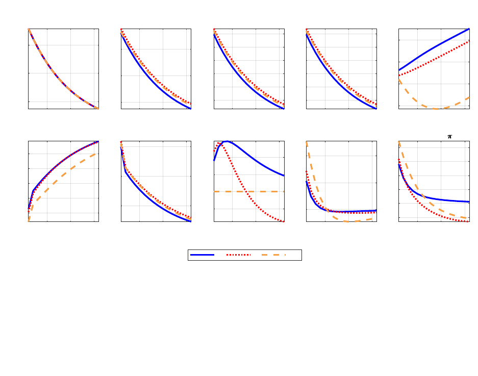
on labor markets generates an increase in real wages and, thus, in firms’ marginal costs. We see a
combination of these effects in equilibrium, so salaries, labor, and output also increase.
5 10 15
quarters
5
10
15
CB purchases (b
L,CB
)
5 10 15
quarters
5
10
15
CB balance sheet/y
5 10 15
quarters
4
6
8
10
12
14
Reserves (b
S,FI
)
5 10 15
quarters
4
6
8
10
12
14
Deposits (d)
5 10 15
quarters
-3
-2.5
-2
-1.5
HH long-debt (b
L,H
)
5 10 15
quarters
-60
-50
-40
-30
-20
Term Spread
5 10 15
quarters
5
10
15
Equity (A)
5 10 15
quarters
-0.1
0
0.1
0.2
Interest rate (R)
5 10 15
quarters
0
0.2
0.4
Output (y)
5 10 15
quarters
-0.2
0
0.2
0.4
0.6
0.8
Inflation ( )
M F ZLB
Figure 5: Impact of a Quantitative Easing shock conditional on a regime
Note: log deviations (in %) in a simulated path with a one standard deviation shock in the
central bank purchases of long-term bonds (ϵ
QE
t
= 1) to the counterfactual path without
shock (ϵ
QE
t
= 0). Path conditional on the monetary-led regime (continue blue line),
fiscally-led regime (dotted red line), and zero lower bound regime (dashed yellow line) for 16
periods. The balance sheet to output ratio, interest rates, and inflation are annualized.
The intensity of these expansionary effects critically depends on the regime, being more expan-
sive at the ZLB and, in second place, in the fiscally-led regime. At the ZLB, the fixed short-term
interest rate exacerbates the substitution effect between savings and consumption. The short-term
nominal interest rate increases in the fiscal and monetary-led regimes, following the corresponding
Taylor rule. This return increase ameliorates the expansionary and inflationary effects of an increase
in central bank purchases, especially in the monetary-led regime where the real short-term interest
rate becomes positive.
Figure 6 shows the fiscal variables. Government debt behavior depends on the evolution of the
three components of the government budget constraint: fiscal surplus, central bank remittances to
the treasury, and debt service. First, the expansionary effect of central bank purchases triggers a
35
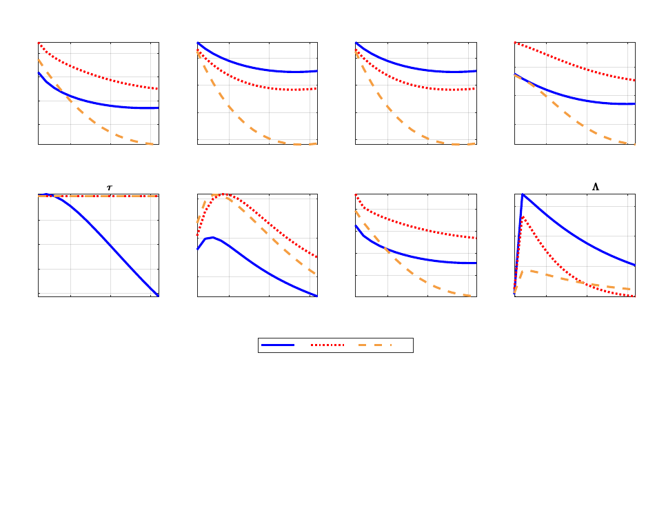
fall in government spending due to automatic stabilizers. Hence, primary fiscal surplus increases
on impact in all regimes. This effect is more significant in the ZLB, where output increases more.
Central bank profits (Λ
CB
t
) increase from period two in all scenarios, alleviating the pressure on
fiscal accounts. Finally, total debt service behavior differs among regimes. Initially, it falls due to
larger fiscal surpluses and remittances from the central bank, allowing the treasury to issue less
debt (b
L
t
, b
S
t
). This effect is larger in the ZLB and fiscally led regime, where higher inflation rates
give the government seigniorage revenues. However, the revaluation of long-term bonds is so strong
in the fiscally-led regime that it dominates the effect on real debt (b
t
), which increases.
The final result is an increase in fiscal space, interpreted as a fall in real debt (b
t
) at the ZLB and
the monetary regime. This effect is milder in the second, where taxes fall following debt issuance.
In the fiscally-led regime, however, the revaluation effect on long-term bonds is so strong that the
debt ratio to GDP increases.
5 10 15
quarters
-1
-0.5
0
0.5
Real debt (b)
5 10 15
quarters
-2
-1.5
-1
-0.5
Short-term debt (b
S
)
5 10 15
quarters
-2
-1.5
-1
-0.5
Long-term debt (b
L
)
5 10 15
quarters
-1
-0.5
0
Debt to GDP
5 10 15
quarters
-0.4
-0.3
-0.2
-0.1
0
Tax ( )
5 10 15
quarters
0
5
10
P. fiscal surplus
5 10 15
quarters
-1
-0.5
0
0.5
Debt service
5 10 15
quarters
0
100
200
300
CB Profits (
CB
)
M F ZLB
Figure 6: Impact of a Quantitative Easing shock conditional on a regime: fiscal variables
Note: log deviations (in %) in a simulated path with a one standard deviation shock in the
central bank purchases of long-term bonds (ϵ
QE
t
= 1) to the counterfactual path without
shock (ϵ
QE
t
= 0). Path conditional on the monetary-led regime (continue blue line),
fiscally-led regime (dotted red line), and zero lower bound regime (dashed yellow line) for 16
periods. Debt to GDP is annualized.
36
This exercise shows that the expansionary effects of QE policies are of considerate size under
a crisis regime. At the ZLB, 1.3p.p. temporal increase in the central bank balance sheet increases
output by almost 0.6 p.p. and inflation 0.9p.p. to the counterfactual scenario without intervention.
However, its effects on output and inflation are milder in fiscal and monetary dominance regimes,
where output increases by 0.3 and 0.2 p.p. and inflation by 0.6 and 0.5p.p., being considerably less
persistent in the first case. This analysis provides some insights into the power of QE to expand
the economy and how it differs among regimes. Furthermore, it highlights the fact that the fiscal
implication of this policy entails substantial differences across policy scenarios.
7 Exit strategies from Quantitative easing programs
As stated by policymakers, financial analysts, and academics, there is high uncertainty regarding
the impact of implementing Quantitative Easing programs and, even more, the unwinding of the
economic stimulus introduced through these measures. The main objective of this paper is to
contribute to understanding the macroeconomic effects of different strategies regarding the size of
the central bank balance sheet. In this section, I simulate the economy to generate a crisis that
resembles the one in the US from the first quarter of 2020 when the COVID-19 pandemic became
widespread worldwide. First, I show the model can generate a crisis with similar characteristics
to the data: a substantial fall in output and short-term interest rate until it reaches the zero
lower bound, together with a rise in the debt-to-GDP ratio and a fall in the inflation rate. In
this context, I simulate a Quantitative Easing program that increases the ratio of the central bank
balance sheet over output by 10p.p. and compare the macroeconomic dynamics with and without
this program. Then, I study three different strategies for managing the central bank balance sheet
size: 1) maintaining the enlarged size after the crisis (Tapering), 2) decreasing the balance sheet
size: a) by letting the bonds that mature, run off the balance sheet (Quantitative Tightening (QT)),
and b) at a faster speed by selling bonds (Aggressive QT ).
Tapering is defined as a situation where the stock of long-term bonds at the central bank (b
L,CB
t
)
remains constant, implying b
L,CB
t
= b
L,CB
t−1
. With that objective, the central bank engages in new
purchases of bonds to make up for maturing bonds. The size of the central bank balance sheet over
output ratio is, however, endogenous since it is affected by the price of long-term bonds (Q
L
t
) and
output y
t
, which are not under the control of the central bank.
37

Quantitative tightening is a strategy where the central bank does not repurchase the bonds that
mature every period, letting them run off the balance sheet. The stock of bonds at the central
bank will then decrease at rate δ, the average maturity of long-term bonds, the unique kind of
bonds the monetary authority purchases in the model. This implies the stock of bonds follows:
b
L,CB
t
= (1 − δ) b
L,CB
t−1
.
Finally, the strategy called Aggressive QT consists of the central bank actively selling public
bonds. It is any path of shocks that generates b
L,CB
t
< (1 − δ) b
L,CB
t−1
, implying that the stock of
bonds at the central bank decreases at a faster rate than the maturity rate.
7.1 The crisis development and the QE program
I simulate the model in 50,000 samples of 40 periods under two scenarios, “Baseline” and “Quantita-
tive Easing,” with the following characteristics. In the baseline, the economy is at the approximation
point at t=1, and in the monetary-led regime. During periods 2 to 4, the economy is hit by strong
negative preference and TFP shocks. Since both shocks are persistent, they remain below their
steady state value for the whole sample. From t=2 onward, the regime at place is stochastic, follow-
ing the transition matrix presented in section 3.8. This scenario makes QE, monetary policy, and
fiscal policy shock random. After the initial hit during periods 2 to 4, preference and TFP shocks
follow random paths.
The quantitative easing scenario shares the same characteristics as the baseline, except that the
path for QE shocks is not random. It is imposed to generate an increase in the annualized central
bank balance sheet to 20% of GDP. in the first six periods. After period 6, the balance sheet remains
constant (tapering strategy).
Figures 7 and 8 show the mean of simulated variables for the first 20 periods for the economy
without QE (continuous blue line) and with QE (dotted orange line). The negative preference and
technology shocks generate a substantial fall in output growth that reaches its bottom of -8.8p.p. in
period four. Besides, it does not fully recover for eight periods. The short-term interest rate starts
falling immediately until it reaches the ZLB. The primary fiscal surplus falls by almost 6p.p. in the
baseline scenario.
26
26
This exercise aims to analyze the effects of the quantitative easing program. This baseline exercise
excludes the increase in fiscal transfers that took place during that period of turmoil. In the model, it can
be easily generated through a fiscal shock in g
t
, generating more significant primary fiscal deficits.
38
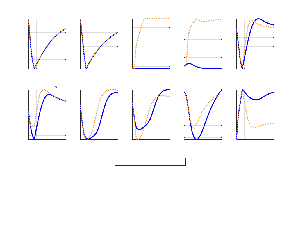
The main features of the crisis with quantitative easing are the following. First, there is a
slightly milder fall in output than without the program. Second, there is a faster recovery within
less than a year. QE also has expansionary effects in terms of inflation. Prices fall less during the
crisis than in a scenario without the intervention of the central bank, however, this is at the cost of
more important inflationary dynamics in the recovery. Inflation reaches a peak of 8.4% in period
nine, two periods after the balance sheet reaches its maximum value of 20.8% of GDP. Without this
program, inflation increases less during the recovery and reaches a peak of 6.9% three periods later.
5 10 15 20
quarters
0.7
0.8
0.9
1
Pref shock
5 10 15 20
quarters
0.94
0.96
0.98
1
TFP shock
5 10 15 20
quarters
0.015
0.02
0.025
0.03
0.035
Treasuries in CB
5 10 15 20
quarters
10
15
20
%
CB Bal. sheet/GDP
5 10 15 20
quarters
-8
-6
-4
-2
0
2
%
Output growth
5 10 15 20
quarters
-5
0
5
%
Inflation ( )
5 10 15 20
quarters
0
2
4
%
Interest rate (R)
5 10 15 20
quarters
0
2
4
6
%
Long-run yield (R
L
)
5 10 15 20
quarters
-6
-4
-2
0
%
P. fiscal surplus/GDP
5 10 15 20
quarters
80
85
90
%
Debt/GDP
Crisis Crisis + QE
Figure 7: Simulated crisis
Note: Average from 50,000 samples. The continuous blue line is the scenario without the QE
program. The Orange dotted line is the scenario with a QE program that increases the
annualized central bank balance sheet to output by around 13p.p. Interest rate (R), long-run
return (R
L
), and inflation are annualized gross rates. Debt-to-GDP is annualized.
In both cases, real debt increases quickly when the crisis starts, increasing almost 20p.p. of GDP.
However, its real value decreases fast following the output and price recovery. The fall in real debt
is more significant under the QE program for three reasons: first, central bank purchases increase
central bank profits transferred to the treasury; second, the central bank intervention decreases
the long-run yield, and thus interest payments on debt are lower; and third, the faster recovery
39
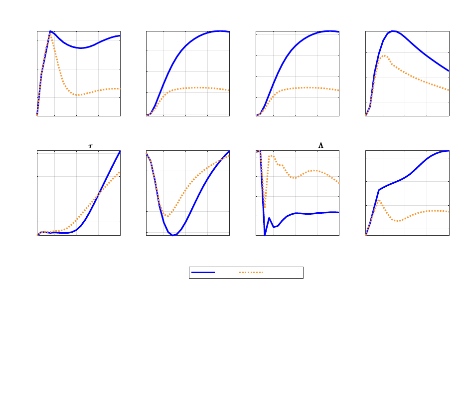
triggers a fall in government spending driven by automatic stabilizers so that the primary fiscal
deficit is lower. These three factors allow the government to issue less debt during the crisis than
in a counterfactual without the QE program.
5 10 15 20
quarters
0
0.5
1
1.5
%
CB profits/GDP (
CB
)
5 10 15 20
quarters
14
15
16
17
%
Interest payments/GDP
5 10 15 20
quarters
80
85
90
%
Debt/GDP
5 10 15 20
quarters
0.07
0.075
0.08
0.085
b
S
5 10 15 20
quarters
0.15
0.16
0.17
0.18
b
L
5 10 15 20
quarters
0.05
0.06
0.07
New debt issuance
5 10 15 20
quarters
0.22
0.225
0.23
0.235
Taxes ( )
5 10 15 20
quarters
-6
-4
-2
0
%
P. fiscal surplus/GDP
Crisis Crisis + QE
Figure 8: Simulated crisis
Note: Average from 50,000 samples. The continuous blue line is the scenario without the QE
program. The Orange dotted line is the scenario with a QE program that increases the
annualized central bank balance sheet to output by around 10p.p.
Finally, figure 9 shows, per period, the percentage of samples in which the economy is at the
ZLB regime. Notice it is zero in periods one (initial condition) and two. The reason is that the
endogenous probability of moving to the zero lower bound regime at t + 1 depends on the interest
rate at t. From period three onward, the economy is at the ZLB with a high probability. The
frequency of this regime is considerably lower under the scenario with the QE program, and it is
almost nil from period twelve.
40

2 4 6 8 10 12 14 16 18 20
Quarter
0
10
20
30
40
50
60
70
80
90
%
Crisis Crisis + QE
Figure 9: Frequency ZLB regime
Note: Percentage of simulated samples at the ZLB regime, per period, from 50,000 samples,
in the scenario without the QE (continuous blue line), and with QE program (orange dotted
line).
To summarize, unconventional monetary policy intervention reduces the severity of the crisis
and implies a faster recovery and a shorter duration of the ZLB regime. Additionally, the debt stock
is lower while inflation is higher.
7.2 Central bank balance sheet exit strategies
This section compares the path for endogenous variables under three scenarios after the initial crisis.
The continuous green line is the scenario with Quantitative Tightening (QT) from period 9 onward,
where the central bank allows mature treasuries to run off its balance sheet. Light-blue dashed line
41
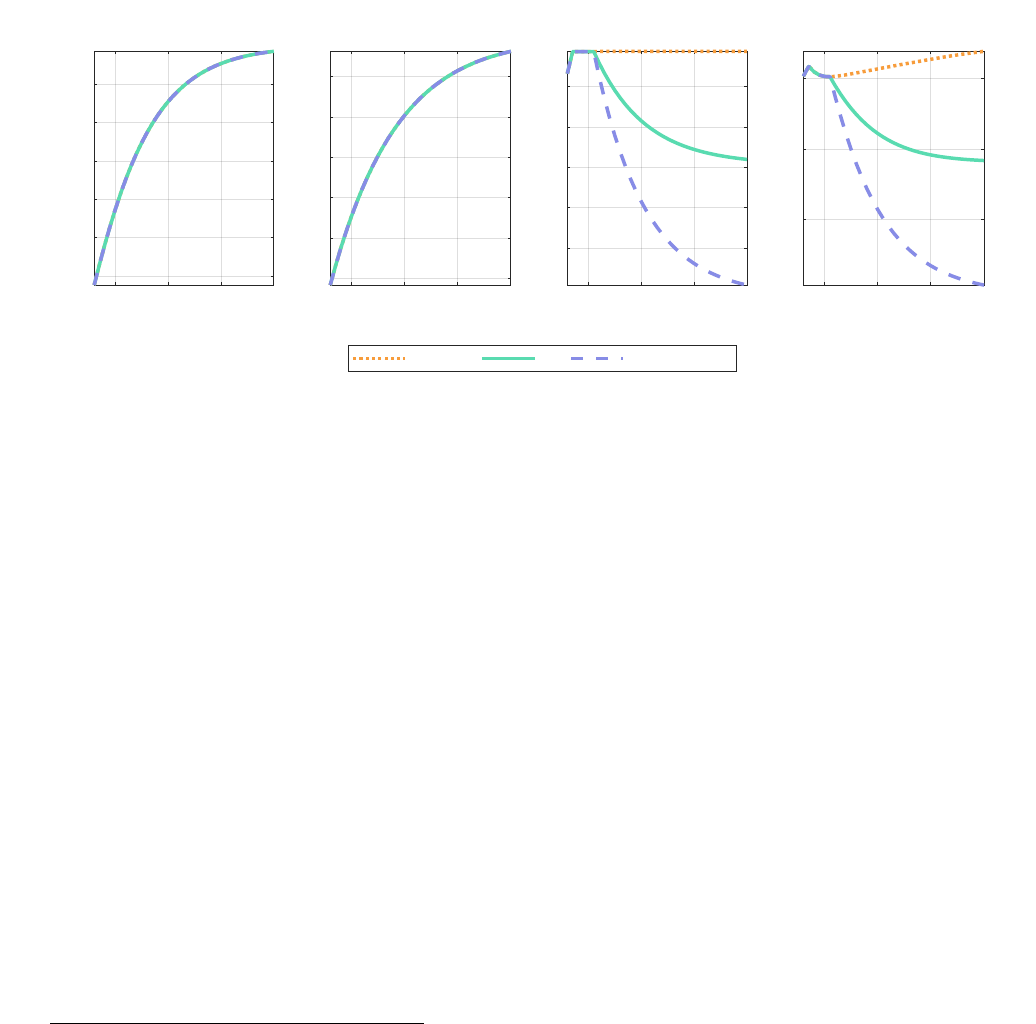
is the scenario with sales of bonds from period 9 onward.
2728
The orange dotted line corresponds
to Tapering, identical to the one in figure 7. Figure 10 shows the evolution of the treasuries in the
central bank (b
L,CB
t
) and the central bank balance sheet (Q
L
t
b
L,CB
t
) as a GDP ratio.
10 20 30 40
quarters
0.7
0.75
0.8
0.85
0.9
0.95
Pref shock
10 20 30 40
quarters
0.94
0.95
0.96
0.97
0.98
0.99
TFP shock
10 20 30 40
quarters
0.015
0.02
0.025
0.03
0.035
Treasuries in CB
10 20 30 40
quarters
10
15
20
CB Balance sheet/y(%)
Tapering QT Aggressive QT
Figure 10: Crisis and exit strategies from QE.
Note: Average from 50,000 samples, plots since period t=8. The Orange dotted line is the
tapering scenario. The continuous green line is the scenario with Quantitative Tightening
(QT) from period 9 onward. Light-blue dashed line is the scenario with Aggressive QT or
sales of bonds from period 9 onward.
The figure shows mean values for each variable across samples. This implies an average behavior
where the regime is stochastic, i.e., which could leave the ZLB regime towards a fiscally-led regime
or a monetary-led regime following the ergodic probabilities of matrix presented in section 3.8.
For clarity of exposition, I show the variables from period t=8. The unwinding of the balance
sheet is assumed to start almost two years after the crisis when most of the simulated samples are
endogenously out of the ZLB (as shown in figure 4).
29
When the central bank unwinds its balance sheet, it decreases the total demand for long-term
bonds, pushing their price down, and generating a rise in the long-term yield. This price effect causes
incentives in households to rebalance its portfolio away from deposits and toward long-term public
bonds. At the same time, since households were already investors in these assets, they perceive a
27
For this scenario, I assume a QE shock equal to -0.2 for every t from t=9.
28
The policies denominated “QT” and “Aggressive QT” in this paper have been classified as “Passive QT”
and “Active QT” by the Bank of England. See, for instance, the speech of Andrew Hauser at the ECB’s 2022
Conference on Money Markets, available at: www.bis.org/review/r221104k.pdf.
29
The main results are robust to start the unwinding of the central bank balance sheet some periods after
(period t = 12 or t = 15). These exercises are available under request.
42
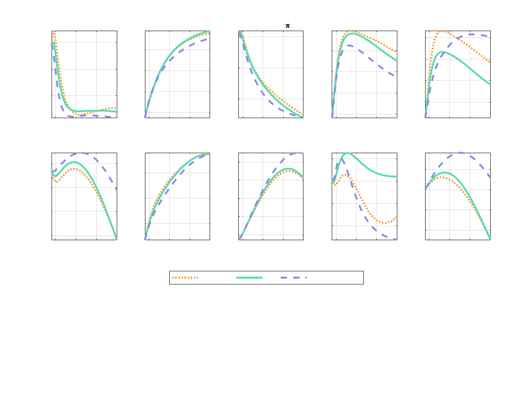
negative wealth effect from the revaluation of their portfolio, decreasing consumption and aggregate
demand in the economy, to a situation without the QT. This effect complements the substitution
effect that generates incentives to save more in the context of rising interest rates.
10 20 30 40
quarters
0.5
1
1.5
%
Output growth
10 20 30 40
quarters
0.72
0.74
0.76
0.78
Consumption
10 20 30 40
quarters
4
6
8
%
Inflation ( )
10 20 30 40
quarters
2
3
4
5
%
Interest rate (R)
10 20 30 40
quarters
3
4
5
6
%
Long-run return (R
L
)
10 20 30 40
quarters
76
78
80
82
%
Debt/GDP
10 20 30 40
quarters
-2
0
2
%
P.Fiscal Surplus/GDP
10 20 30 40
quarters
0.22
0.225
0.23
0.235
0.24
Taxes
10 20 30 40
quarters
0
0.5
1
1.5
%
CB profits/GDP
10 20 30 40
quarters
0.135
0.14
0.145
0.15
Interest payments
Tapering QT Aggressive QT
Figure 11: Crisis and exit strategies from QE.
Note: Average from 50,000 samples, since period t=8. The Orange dotted line is the tapering
scenario. The continuous green line is the scenario with Quantitative Tightening (QT) from
period 9 onward. Light-blue dashed line is the scenario with Aggressive QT or sales of bonds
from period 9 onward. Output growth, balance sheet, and Debt to GDP are in percentages.
Interest rate (R), long-run return (R
L
), inflation, and debt-to-GDP are annualized.
Firms respond to this fall in aggregate demand through a combination of a fall in production
and prices. In this context, unwinding the central bank balance sheet generates a fall in output
growth and faster inflation stabilization, allowing the central bank to stop increasing the short-term
nominal interest rate. The disinflationary forces of reducing the central bank balance sheet are more
substantial as the unwinding speed gets faster. Under an aggressive QT, after four years of applying
this strategy (period t=27) and in the absence of further shocks, the inflation rate is 3.3%, while
it remains at 4.1% under Tapering. Moreover, this is accomplished with a short-term interest rate
43
of 1p.p. lower than in the tapering scenario. In a longer horizon (40 periods from the beginning
of the simulation), we can see that the inflation rate remains at a higher level when the size of the
balance sheet remains constant after the expansion during the crisis. In other words, more liquidity
permanently circulating in the economy increases the long-term inflation rate.
On the fiscal side, we observe that the debt stock increases with the balance sheet unwinding.
There are three reasons. First, the negative effects on output trigger government spending through
automatic stabilizers, decreasing the fiscal surplus even as taxes increase. Second, interest payments
increase due to higher interest rates. Third, central bank remittances to the treasury decrease in the
scenario of sales of bonds. Notice that when the short-term interest rate increases, the central bank
starts paying interest rates on reserves, decreasing its profits. With the unwinding, bank reserves
which constitute the liabilities in its balance sheet, decline, reducing this cost. However, at the
same time, it generates a fall in the return it receives for its holdings of long-term bonds. Under
QT, the first effect dominates, and central bank profits increase compared to the tapering scenario.
The opposite happens in an aggressive QT, where the unwinding is faster.
In conclusion, selling bonds from the central bank effectively reduce the inflation rate to the
target, requiring smaller increases in the short-term interest rate. However, it has the downside
of a slower deleveraging of the economy. As I show in the next section, these conclusions are not
independent of the policy regime at the time of the unwinding.
7.3 Unwinding the balance sheet in a fiscally-led regime
In this section, I restrict the analysis to the samples that exit the ZLB toward a fiscally-led regime
and stay there for at least one year (4 quarters). I compare it with the selected samples where the
exit from the ZLB is toward the monetary regime. Since both fiscally and monetary-led regimes are
substantially persistent, the probability of staying there for a good proportion of the sample is high.
The exit of the crisis regime is stochastic and could happen at any period. I present the dynamics
corresponding to these subsamples in figures 12 and 13.
44
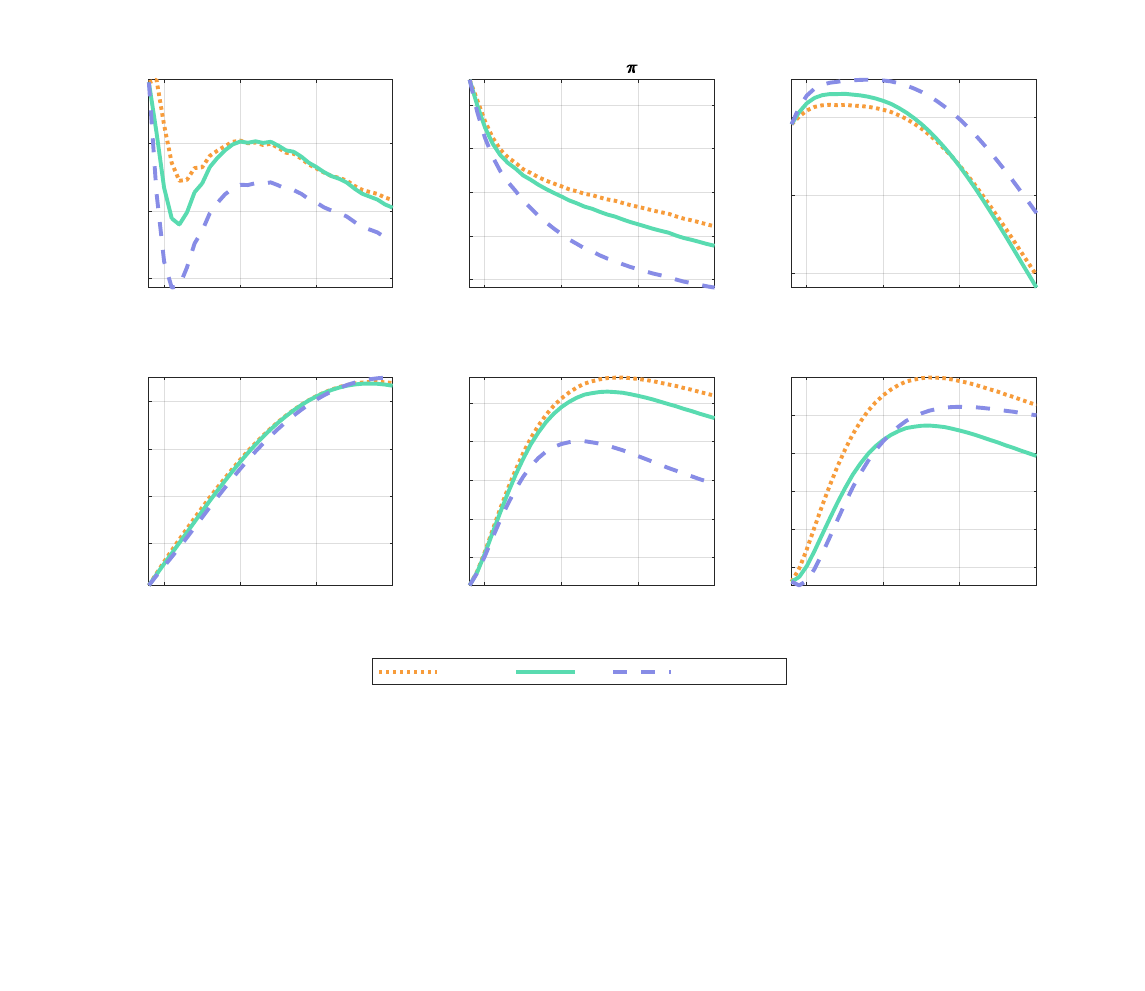
10 20 30 40
quarters
1
2
3
4
5
%
Interest rate (R)
10 20 30 40
quarters
2
3
4
5
6
%
Inflation ( )
10 20 30 40
quarters
75
80
85
%
Debt/GDP
10 20 30 40
quarters
-2
0
2
4
%
P. fiscal surplus/GDP
10 20 30 40
quarters
0
0.2
0.4
%
Output growth
10 20 30 40
quarters
1
2
3
4
5
%
Long-run return (R
L
)
Tapering QT Aggressive QT
Figure 12: Quantitative Tightening in the monetary-led regime.
Note: Simulation of 50,000 samples, since period t=8. The figure restricts the analysis to
samples that exit the zero lower bound toward a monetary-led regime and stay there for at
least one year (4 quarters). The Orange dotted line is the tapering scenario, the same as the
one in figure 7. The continuous green line is the scenario with Quantitative Tightening (QT)
from period 9 onward. Light-blue dashed line is the scenario with Aggressive QT or sales of
bonds from period 9 onward. Debt to GDP is in percentages. Interest rate (R), long-run
return (R
L
), inflation, and debt-to-GDP are annualized.
Exiting the crisis towards a fiscally-led regime brings a higher inflation rate that peaks at 11% in
period nine and an expansionary period where output growth is above trend. As a result, interest
rates are higher, even under lower reactions to inflation and output deviations. Higher inflation
rates help to quickly reduce the stock of real debt, which falls 20p.p. of GDP in 7 quarters.
The most remarkable difference between regimes is that QT in a fiscally-led regime has little
impact on inflation, while it has a sizable disinflationary impact in a monetary-led regime. In a
monetary-led regime, the inflation rate in scenarios with QT is persistently below the one in the
case with tapering. This difference tops at 1.5p.p. Notice that this is attained with lower increases
45
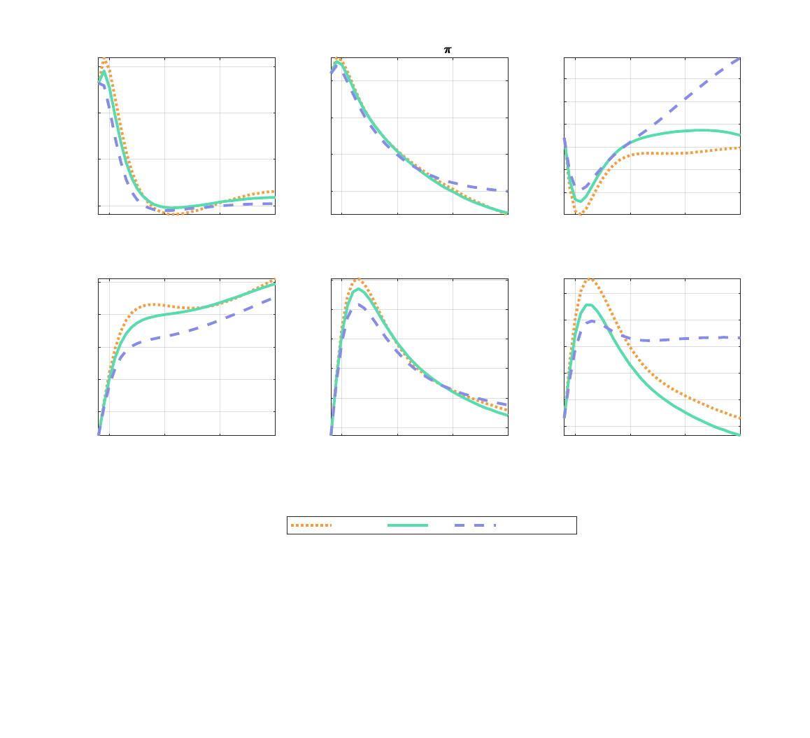
in the short-term interest rate. In the case of aggressive QT, the conventional monetary policy tool
changes the stance from contractionary to expansionary 10 quarters before the case of constant size
in the central bank balance sheet. Figure 14 shows the accumulated inflation since period t = 8
in both regimes under the alternative scenarios. In the monetary-led regime, the aggressive QT
reduces accumulated inflation by 34% at quarter 40.
10 20 30 40
quarters
4
5
6
7
8
9
%
Interest rate (R)
10 20 30 40
quarters
4
6
8
10
%
Inflation ( )
10 20 30 40
quarters
75
76
77
78
79
80
%
Debt/GDP
10 20 30 40
quarters
-2
-1
0
1
2
%
P. fiscal surplus/GDP
10 20 30 40
quarters
0
1
2
3
%
Output growth
10 20 30 40
quarters
4
5
6
7
8
9
%
Long-run return (R
L
)
Tapering QT Aggressive QT
Figure 13: Quantitative Tightening in the fiscally-led regime.
Note: Simulation of 50,000 samples, since period t=8. The figure restricts the analysis to
samples that exit the zero lower bound toward a fiscally-led regime and stay there for at least
one year (4 quarters). The Orange dotted line is the tapering scenario, the same as the one in
figure 7. The continuous green line is the scenario with Quantitative Tightening (QT) from
period 9 onward. Light-blue dashed line is the scenario with Aggressive QT or sales of bonds
from period 9 onward. Debt to GDP is in percentages. Interest rate (R), long-run return
(R
L
), inflation, and debt-to-GDP are annualized.
The difference in inflationary dynamics after QT programs is the following. As shown in the
average scenario, real debt increases with QT. In the monetary-led regime, the increase in debt
causes a rise in taxes, given by the fiscal rule. This exacerbates the fall in aggregate demand and
46
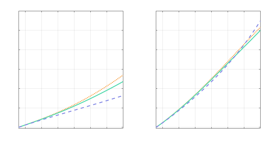
the disinflationary effects of QT. In the fiscally-led regime, the rise in public debt increases actual
and expected inflation, aggravating the rise in yield spreads and mitigating the disinflationary effects
of QT. In this case, the negative demand effect driven by the reduction in central bank purchases
is not enough to counteract the stimulative impact of negative interest rates and fiscal stimulus.
10 15 20 25 30 35 40
quarters
1
2
3
4
5
6
7
Price level
Monetary regime
10 15 20 25 30 35 40
quarters
1
2
3
4
5
6
7
Fiscal regime
Figure 14: Accumulated inflation under different regimes and exit strategies from QE.
Note: Simulation of 50,000 samples, since period t=6. The figure restricts the analysis to
samples that exit the zero lower bound toward a monetary (left) or fiscally-led regime (right)
and stay there for at least one year (4 quarters). The continuous green line is the scenario
with Quantitative Tightening (QT) from period 9 onward. Light-blue dashed line is the
scenario with Aggressive QT or sales of bonds from period 9 onward. This figure shows the
CPI in the monetary vs. fiscal regime, with base P
8
= 1.
In conclusion, in a regime where the fiscal authority is not committed to stabilizing the govern-
ment debt, unwinding the central bank balance sheet does not generate clear economic advantages.
8 Concluding Remarks
I study different exit strategies for reducing the central bank balance sheet in a model that generates
fiscal-monetary policy trade-offs.
47
The impact of central bank balance sheet policies (QE or QT) depends on the fiscal-monetary
policy mix. First, QE reduces the need for new debt issuance. Second, as a counterpart of the central
bank’s balance sheet expansions, liquidity increases substantially, both in the hand of commercial
banks (reserves) and non-bank private agents (deposits). The extent to which the increase in
liquidity affect output and inflation rate depends on the fiscal-monetary policy mix. QE is more
expansive at the ZLB and under the fiscally-led regime when the inflationary impact is also more
significant.
How the central bank balance sheet’s size is reduced matters for inflation, output, and debt
dynamics. In an average simulation, when the monetary authority starts shrinking its holdings of
long-term government bonds, it decreases inflation at the cost of an increase in the ratio of debt to
GDP. These effects increase when the exit strategy is more aggressive.
When the unwinding occurs in a fiscally-led regime, reducing the balance sheet’s size does not
help bring the inflation back to target. In this regime, the rise in public debt increases actual and
expected inflation, exacerbating the rise in yield spreads and mitigating the disinflationary effects
of QT. This implies that, with unconventional policies, coordination between fiscal and monetary
authorities is necessary to stabilize the inflation rate.
48
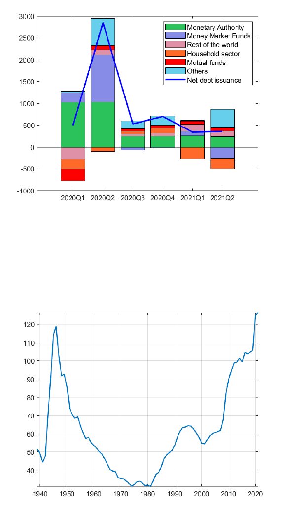
9 Appendix
9.1 Extra plots for US case
Figure 15: Change in Treasuries’ holdings
Source: US Financial Accounts. Data in billions of dollars. Contain revaluation effects.
Figure 16: Public debt to GDP in US: historical perspective
Source: FRED. Annual Gross Federal Debt as a Percent of GDP.
49
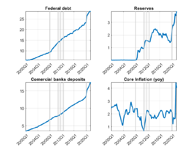
Figure 17: Macroeconomic variables: public debt, liquidity, inflation. Great recession and
COVID-19 crisis.
US Federal Debt, Reserves and Deposits, in trillions of dollars. Core inflation in %. Source
debt, deposits and inflation data: FRED. Source reserves: US financial accounts, release
December 2021.
9.2 Model: Financial intermediary optimization problem
The optimization problem of a representative financial intermediary can be written in sequential
form as follows:
V
I
W
I
t
= max
A
t
,D
I
t
,F
I
t
,B
S,I
t
τ
I
W
I
t
− A
t
+ E
t
M
t,t+1
V
I
W
I
t+1
s.t. (1 − τ
I
)W
I
t
+ A
t
− Φ
A
(A
t
) + Q
D
t
D
I
t
= Q
S
t
B
S,I
t
W
I
t
= B
S,I
t−1
− D
I
t−1
D
I
t
≤ ζB
S,I
t
50

Define η
t
as the Balance sheet multiplier and µ
t
as the Leverage constraint multiplier. The first
order conditions are given by the following system:
A
t
: − 1 + η
t
− η
t
χ
A
t
P
t
= 0
D
I
t
: η
t
Q
D
t
− µ
t
− E
t
M
t,t+1
V
I
w
W
I
t+1
= 0
B
S,I
t
: − η
t
Q
D
t
+ µ
t
ζ + E
t
M
t,t+1
V
I
w
W
I
t+1
= 0
And the envelope condition:
V
I
w
W
I
t+1
= τ
I
+ η
t
(1 − τ
I
)
Using the first order condition with respect to A
t
to substitute out the multiplier η
t
, we obtain
the system of equations that characterize the financial intermediary’s optimization problem, together
with 7, 8, 9, ??:
Q
D
t
= E
t
˜
M
t,t+1
+ µ
t
(1 − χa
t
) (22)
Q
S
t
= E
t
˜
M
t,t+1
+ ζµ
t
(1 − χa
t
) (23)
Where
˜
M
t,t+1
is the stochastic discount factor for financial intermediaries, defined as:
˜
M
t,t+1
≡ M
t,t+1
1 − χ
A
t
P
t
τ
I
+
1 − τ
I
1 − χ
A
t+1
P
t+1
!
9.3 Equilibrium conditions
In this section I present the system of equilibrium conditions with functional forms and in real
terms.
Definitions: d
t
=
D
t
P
t
, b
j,i
t
=
b
j,i
t
P
t
, w
t
=
W
t
P
t
, div
t
=
Div
t
P
t
, π
f
t
=
Π
f
t
P
t
, a
t
=
A
t
P
t
, mc
t
=
MC
t
P
t
, w
I
t
=
W
I
t
P
t
,
π
t
=
P
t
P
t−1
, for j ∈ {L, S}, i ∈ {H, CB, F I}.
9.3.1 Households
c
t
+ Q
D
t
d
H
t
+ b
L,H
t
Q
L
t
= w
t
n
t
− τ
t
+
d
H
t−1
π
t
+
b
L,H
t−1
π
t
κ + (1 − δ)Q
L
t
+ div
t
+ π
f
t
+
χ
2
a
2
t
(1)
51

γn
η
t
h
c
1−φ
t
d
H
t
φ
i
−σ
(1 − φ)c
−φ
t
(d
H
t
)
φ
= w
t
(2)
Q
D
t
= E
t
M
t,t+1
+
φc
t
(1 − φ)d
H
t
(3)
Q
L
t
+ ϕ
L
b
L,H
t
(b
L,H
)
2
= E
t
M
t,t+1
κ + (1 − δ)Q
L
t+1
(4)
M
t,t+1
=
βλ
t+1
λ
t
= βE
t
ν
t+1
ν
t
h
c
1−φ
t+1
d
H
t+1
φ
i
−σ
c
−φ
t+1
(d
H
t+1
)
φ
h
c
1−φ
t
d
H
t
φ
i
−σ
c
−φ
t
(d
H
t
)
φ
1
π
t+1
(5)
9.3.2 Firms
y
t
= z
t
n
t
(6)
π
f
t
= y
t
− w
t
n
t
−
ϕ
P
2
(π
t
− 1)
2
y
t
(7)
1 − ε + εmc
t
= ϕ
P
(π
t
− π
∗
) π
t
− ϕ
P
E
t
M
t,t+1
y
t+1
y
t
π
2
t+1
(π
t+1
− π
∗
)
(8)
w
t
= mc
t
z
t
(9)
9.3.3 Financial intermediaries
div
t
= τ
I
w
I
t
− a
t
(10)
(1 − τ
I
)w
I
t
+ a
t
−
χ
2
a
2
t
+ Q
D
t
d
I
t
= Q
S
t
b
S,I
t
(11)
w
I
t
=
b
S,I
t−1
π
t
−
d
I
t−1
π
t
(12)
d
I
t
≤ ζb
S,I
t
(13)
Q
D
t
= E
t
˜
M
t,t+1
+ µ
t
(1 − χa
t
) (14)
Q
S
t
= E
t
˜
M
t,t+1
+ ζµ
t
(1 − χa
t
) (15)
˜
M
t,t+1
= M
t,t+1
(1 − χa
t
)
τ
I
+
1 − τ
I
1 − χa
t+1
(16)
52

9.3.4 Government
1
R
t
= Q
S
t
(17)
Q
S
t
b
S,CB
t
+ Q
L
t
b
L,CB
t
= 0 (18)
b
t
= Q
S
t
b
S
t
+ Q
L
t
b
L
t
(19)
b
S
t
= (1 − ¯µ)/¯µb
L
t
(20)
g
t
= θ(y
∗
− y
t
) + (1 − ρ
g
)¯g + ρ
g
g
t−1
+ σ
g
ε
g
t
, ε
g
t
∼ N(0, 1) (21)
9.3.5 Market clearing conditions
c
t
+ g
t
+
ϕ
P
2
(π
t
− π
∗
)
2
y
t
= y
t
(22)
d
H
t
= d
I
t
(23)
b
S
t
= b
S,I
t
+ b
S,CB
t
(24)
b
L
t
= b
L,H
t
+ b
L,CB
t
(25)
9.3.6 Policy rules
τ
t
− τ
∗
= ρ
τ
(ξ
t
) (τ
t−1
− τ
∗
) + (1 − ρ
τ
(ξ
t
)) γ (ξ
t
) (b
t−1
− b
∗
) (16)
R
t
R (ξ
t
)
=
R
t−1
R (ξ
t
)
α
R
(ξ
t
)
"
π
t
π
∗
α
π
(ξ
t
)
y
t
y
∗
α
y
(ξ
t
)
#
1−α
R
(ξ
t
)
e
σ
M
(ξ
t
)ϵ
M
t
(27)
b
L,CB
t
= (1 − ρ
QE
)b
L,CB
∗
+ ρ
QE
b
L,CB
t−1
+ σ
QE
ϵ
QE
t
(28)
Law of motion for exogenous processes: z
t
, ν
t
.
Transition matrix for Markov-switching shock ξ
t
.
9.3.7 Definition of auxiliary variables used in figures and tables
Return on long-term bond:
R
L
t,t+1
= E
t
κ + (1 − δ)Q
L
t
Q
L
t+1
53

Convenience yield:
cy
t
= R
t
− E
t
1
M
t,t+1
Annual debt to GDP ratio:
b
t
4y
t
Primary fiscal surplus:
s
t
= τ
t
− g
t
Total interest rate payments:
(R
t−1
− 1)
b
S
t−1
π
t
+ (κ − δ)
b
L
t−1
π
t
Private interest rate payments:
(R
t−1
− 1)
b
S,F I
t−1
π
t
+ (κ − δ)
b
L,H
t−1
π
t
Total debt service:
b
S
t−1
π
t
+ κ
b
L
t−1
π
t
9.4 Steady state and approximation point
At the steady state, shocks are equal to zero: ϵ
ν
t
= 0, ϵ
z
t
= 0, ϵ
g
t
= 0, ϵ
m
t
= 0, ϵ
QE
t
= 0.
Then: z
ss
= 1, ν
ss
= 1, g
ss
= ¯g, b
L,CB,ss
= b
L,CB
∗
.
There is one endogenous variable which steady state value differs among regimes. For monetary
(ξ
C
t
= 0 and ξ
P
t
= M) or fiscal (ξ
C
t
= 0 and ξ
P
t
= F ) dominance regimes, we have: R
t
= R
∗
in
absence of shocks. For the Zero lower bound regime (ξ
C
t
= 1), R
t
= 1.0005. Define p
M
, p
F
, p
C
as the ergodic probability of monetary dominance, fiscal dominance or crisis regime, respectively.
Where: p
M
+ p
F
+ p
C
= 0. The short-term nominal interest rate at the approximation point is
obtained as follows:
R
ss
=
p
M
+ p
F
R
∗
+
1 − p
M
− p
F
1.0005
54
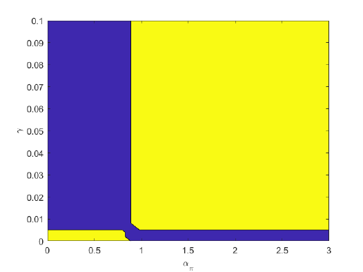
9.5 Additional results
9.5.1 Determinacy regions for fiscal and monetary policy rules
The following figure shows combinations for policy parameters γ and α
π
that give rise to a unique
equilibrium (determinacy, yellow areas), given the calibration for the rest of the parameters, in the
monetary-led regime. The blue areas represent parameter combinations that generate either no
equilibrium, or multiple equilibria.
Figure 18: Determinacy regions
Note: Yellow areas represent combinations of parameters α
π
and γ that give rise to determinacy.
Blue areas represent either multiple equilibria or no equilibrium.
9.5.2 Impulse response functions for additional shocks
This section presents figures showing the impact of the different shocks in the model, under different
regimes. They show log deviations (in %) in a simulated path with a one standard deviation shock,
to the counterfactual path without the shock.
55
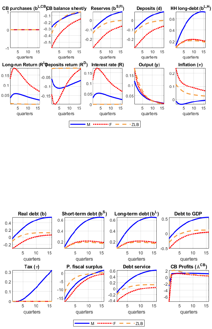
Figure 19: Impact of a Quantitative Easing shock conditional on a regime
Note: log deviations (in %) in a simulated path with a one standard deviation shock in the
government spending (ϵ
g
t
= 1) to the counterfactual path without shock (ϵ
g
t
= 0). Path
conditional on the monetary-led regime (continue blue line), fiscally-led regime (dotted red
line), and zero lower bound regime (dashed yellow line) for 16 periods.
Figure 20: Impact of a Quantitative Easing shock conditional on a regime
Note: log deviations (in %) in a simulated path with a one standard deviation shock in the
government spending (ϵ
g
t
= 1) to the counterfactual path without shock (ϵ
g
t
= 0). Path
conditional on the monetary-led regime (continue blue line), fiscally-led regime (dotted red
line), and zero lower bound regime (dashed yellow line) for 16 periods.
56
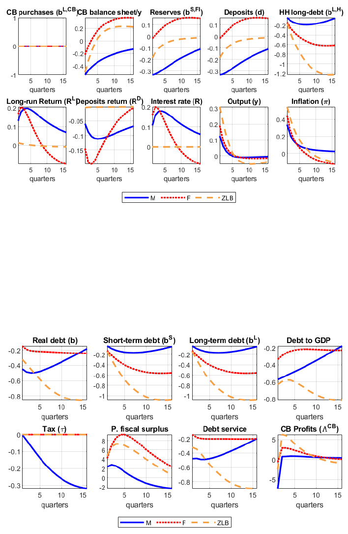
Figure 21: Impact of a Quantitative Easing shock conditional on a regime
Note: log deviations (in %) in a simulated path with a one standard deviation shock in the
preferences (ϵ
ν
t
= 1) to the counterfactual path without shock (ϵ
ν
t
= 0). Path conditional on
the monetary-led regime (continue blue line), fiscally-led regime (dotted red line), and zero
lower bound regime (dashed yellow line) for 16 periods.
Figure 22: Impact of a Quantitative Easing shock conditional on a regime
Note: log deviations (in %) in a simulated path with a one standard deviation shock in the
preferences (ϵ
ν
t
= 1) to the counterfactual path without shock (ϵ
ν
t
= 0). Path conditional on
the monetary-led regime (continue blue line), fiscally-led regime (dotted red line), and zero
lower bound regime (dashed yellow line) for 16 periods.
57

Figure 23: Impact of a Quantitative Easing shock conditional on a regime
Note: log deviations (in %) in a simulated path with a one standard deviation monetary
shock (ϵ
m
t
= 1) to the counterfactual path without shock (ϵ
m
t
= 0). Path conditional on the
monetary-led regime (continue blue line), fiscally-led regime (dotted red line), and zero lower
bound regime (dashed yellow line) for 16 periods.
Figure 24: Impact of a Quantitative Easing shock conditional on a regime
Note: log deviations (in %) in a simulated path with a one standard deviation monetary
shock (ϵ
m
t
= 1) to the counterfactual path without shock (ϵ
m
t
= 0). Path conditional on the
monetary-led regime (continue blue line), fiscally-led regime (dotted red line), and zero lower
bound regime (dashed yellow line) for 16 periods.
58
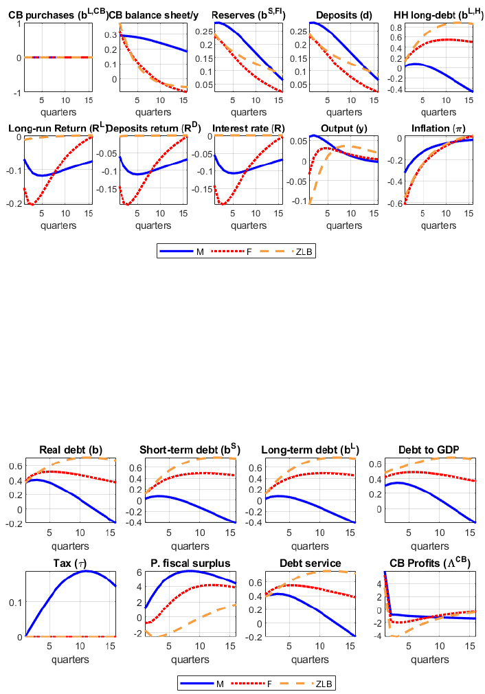
Figure 25: Impact of a Quantitative Easing shock conditional on a regime
Note: log deviations (in %) in a simulated path with a one standard deviation TFP shock
(ϵ
z
t
= 1) to the counterfactual path without shock (ϵ
z
t
= 0). Path conditional on the
monetary-led regime (continue blue line), fiscally-led regime (dotted red line), and zero lower
bound regime (dashed yellow line) for 16 periods.
Figure 26: Impact of a Quantitative Easing shock conditional on a regime
Note: log deviations (in %) in a simulated path with a one standard deviation TFP shock
(ϵ
z
t
= 1) to the counterfactual path without shock (ϵ
z
t
= 0). Path conditional on the
monetary-led regime (continue blue line), fiscally-led regime (dotted red line), and zero lower
bound regime (dashed yellow line) for 16 periods.
59

9.6 Data sources
The following table presents data sources for plots in section 2 and calibration.
Variable Source Table
Deposits in depositary institutions FRED
Monetary aggregate M1 FRED
CPI FRED
US GDP Implicit Price Deflator, Index 2015=100 FRED
Federal reserve Assets US Financial Accounts L109
Federal Reserve Total treasuries US Financial Accounts L110
Federal Reserve Treasury bills US Financial Accounts L111
Federal Reserve Other treasuries US Financial Accounts L112
Federal Reserve Total liabilities US Financial Accounts L113
Federal Reserve Reserves US Financial Accounts L114
Checkable Accounts in Federal Reserve US Financial Accounts L115
Total public debt FRED
Effective federal funds rate FRED
10-year Yield FRED
1-year Yield FRED
US GDP BEA NIPA
Private consumption BEA NIPA
Government spending BEA NIPA
US Population FRED
Table 6: Data sources
60

10 Bibliography
Barthélemy, J. and M. Mar x (2017): “Solving endogenous regime switching models,” Journal
of Economic Dynamics and Control, 77, 1–25.
Barthélemy, J., E. Mengus, and G. Plantin (2021): “The Central Bank, the Treasury, or the
Market: Which One Determines the Price Level?” .
Bassetto, M. (2002): “A game–theoretic view of the fiscal theory of the price level,” Econometrica,
70, 2167–2195.
Bassetto, M. and T. J. Sargent (2020): “Shotgun wedding: Fiscal and monetary policy,”
Annual Review of Economics, 12, 659–690.
Benigno, G. and P. Benigno (2021): “Interest, Reserves, and Prices,” FRB of New York Staff
Report.
——— (2022): “Managing Monetary Policy Normalization,” .
Benigno, G., A. Foerster, C. Otrok, and A. Rebucci (2020): “Estimating macroeconomic
models of financial crises: An endogenous regime-switching approach,” Tech. rep., National Bu-
reau of Economic Research.
Bhattarai, S. and C. J. Neely (Forthcoming): “An Analysis of the Literature on International
Unconventional Monetary Policy,” Journal of Economic Literature.
Bianchi, F. (2013): “Regime switches, agents’ beliefs, and post-World War II US macroeconomic
dynamics,” Review of Economic studies, 80, 463–490.
Bianchi, F., R. Faccini, and L. Melosi (2020): “Monetary and fiscal policies in times of large
debt: Unity is strength,” Tech. rep., National Bureau of Economic Research.
Bianchi, F. and L. Melosi (2017): “Escaping the great recession,” American Economic Review,
107, 1030–58.
——— (2022): “Inflation as a Fiscal Limit,” .
Bocola, L. (2016): “The pass-through of sovereign risk,” Journal of Political Economy, 124, 879–
926.
61

Bonciani, D. and J. Oh (2021): “Optimal monetary policy mix at the zero lower bound,” .
Brunnermeier, M. K., S. A. Merkel, and Y. Sannikov (2020): “The fiscal theory of price
level with a bubble,” Tech. rep., National Bureau of Economic Research.
Chen, H., V. Cúrdia, and A. Ferrero (2012): “The macroeconomic effects of large-scale asset
purchase programmes,” The economic journal, 122, F289–F315.
Cochrane, J. H. (2001): “Long-term debt and optimal policy in the fiscal theory of the price
level,” Econometrica, 69, 69–116.
——— (2021): “The fiscal theory of the price level,” Manuscript. URL.
Cui, W. and V. Sterk (2021): “Quantitative easing with heterogeneous agents,” Journal of
Monetary Economics, 123, 68–90.
Davig, T. and E. Leeper (2008): “Endogenous Monetary Policy Regime Change, NBER Inter-
national Seminar on Macroeconomics 2006,” .
Del Negro, M., G. Eggertsson, A. Ferrero, and N. Kiyotaki (2017): “The great escape? A
quantitative evaluation of the Fed’s liquidity facilities,” American Economic Review, 107, 824–57.
Drechsler, I., A. Savov, and P. Schnabl (2017): “The deposits channel of monetary policy,”
The Quarterly Journal of Economics, 132, 1819–1876.
Elenev, V., T. Landvoigt, P. J. Shultz, and S. Van Nieuwerburgh (2021): “Can Monetary
Policy Create Fiscal Capacity?” Tech. rep., National Bureau of Economic Research.
Foerster, A. T. (2015): “Financial crises, unconventional monetary policy exit strategies, and
agents expectations,” Journal of Monetary Economics, 76, 191–207.
Gaballo, G. and C. Galli (2022): “Asset Purchases and Default-Inflation Risks in Noisy Finan-
cial Markets,” .
Gertler, M. and P. Karadi (2011): “A model of unconventional monetary policy,” Journal of
monetary Economics, 58, 17–34.
Hall, R. E. and R. Reis (2016): “Achieving price stability by manipulating the central bank’s
payment on reserves,” Tech. rep., National Bureau of Economic Research.
62

Harrison, R. (2017): “Optimal quantitative easing,” .
Hatchondo, J. C. and L. Martinez (2009): “Long-duration bonds and sovereign defaults,”
Journal of international Economics, 79, 117–125.
Jordà, Ò., M. Schularick, and A. M. Taylor (2017): “Macrofinancial history and the new
business cycle facts,” NBER macroeconomics annual, 31, 213–263.
Kuttner, K. N. (2018): “Outside the box: Unconventional monetary policy in the great recession
and beyond,” Journal of Economic Perspectives, 32, 121–46.
Leeper, E. M. (1991): “Equilibria under ‘active’and ‘passive’monetary and fiscal policies,” Journal
of monetary Economics, 27, 129–147.
Leeper, E. M. and C. Leith (2016): “Understanding inflation as a joint monetary–fiscal phe-
nomenon,” in Handbook of Macroeconomics, Elsevier, vol. 2, 2305–2415.
Leeper, E. M., C. Leith, and D. Liu (2021): “Optimal time-consistent monetary, fiscal and
debt maturity policy,” Journal of Monetary Economics, 117, 600–617.
Reis, R. (2017): “QE in the future: the central bank’s balance sheet in a fiscal crisis,” IMF Economic
Review, 65, 71–112.
Rotemberg, J. J. (1982): “Sticky prices in the United States,” Journal of political economy, 90,
1187–1211.
Sargent, T. J., N. Wallace, et al. (1981): “Some unpleasant monetarist arithmetic,” Federal
reserve bank of minneapolis quarterly review, 5, 1–17.
Schmitt-Grohe, S., M. Uribe, et al. (2007): “Optimal inflation stabilization in a medium-scale
macroeconomic model,” Monetary policy under inflation targeting, 125–186.
Sims, C. A. (1994): “A simple model for study of the determination of the price level and the
interaction of monetary and fiscal policy,” Economic theory, 4, 381–399.
——— (2016): “Active fiscal, passive money equilibrium in a purely backwardlooking model,”
Manuscript, Princeton University.
63

Sims, E. and J. C. Wu (2021): “Evaluating central banks’ tool kit: Past, present, and future,”
Journal of Monetary Economics, 118, 135–160.
Sims, E., J. C. Wu, and J. Zhang (2020): “The four equation new keynesian model,” The Review
of Economics and Statistics, 1–45.
Wallace, N. (1981): “A Modigliani-Miller theorem for open-market operations,” The American
Economic Review, 71, 267–274.
Wen, Y. et al. (2014): “When and how to exit quantitative easing,” Federal Reserve Bank of St.
Louis Review, 96, 243–265.
64
