The Effect of Shelter-in-Place Orders on Social Distancing and the Spread of the COVID-19 Pandemic: A Study of Texas

University of Texas at Tyler University of Texas at Tyler

Scholar Works at UT Tyler Scholar Works at UT Tyler

Economics Faculty Publications and

Presentations

Social Sciences

11-2020

The Effect of Shelter-in-Place Orders on Social Distancing and the The Effect of Shelter-in-Place Orders on Social Distancing and the

Spread of the COVID-19 Pandemic: A Study of Texas Spread of the COVID-19 Pandemic: A Study of Texas

Marco A. Castaneda

University of Texas at Tyler

, mcastaneda@uttyler.edu

Meryem Saygili

University of Texas at Tyler

, msaygili@uttyler.edu

Follow this and additional works at: https://scholarworks.uttyler.edu/econ_fac

Part of the Social and Behavioral Sciences Commons

Recommended Citation Recommended Citation

Castaneda, Marco A. and Saygili, Meryem, "The Effect of Shelter-in-Place Orders on Social Distancing and

the Spread of the COVID-19 Pandemic: A Study of Texas" (2020).

Economics Faculty Publications and

Presentations.

Paper 1.

http://hdl.handle.net/10950/2802

This Article is brought to you for free and open access by the Social Sciences at Scholar Works at UT Tyler. It has

been accepted for inclusion in Economics Faculty Publications and Presentations by an authorized administrator of

Scholar Works at UT Tyler. For more information, please contact tgullings@uttyler.edu.

ORIGINAL RESEARCH

published: 26 November 2020

doi: 10.3389/fpubh.2020.596607

Frontiers in Public Health | www.frontiersin.org 1 November 2020 | Volume 8 | Article 596607

Edited by:

Nemanja Rancic,

Military Medical Academy, Serbia

Reviewed by:

Cheng-Fang Yen,

Kaohsiung Medical University, Taiwan

Yuriy Timofeyev,

National Research University Higher

School of Economics, Russia

*Correspondence:

Meryem Saygili

[email protected]

Specialty section:

This article was submitted to

Health Economics,

a section of the journal

Frontiers in Public Health

Received: 27 August 2020

Accepted: 05 November 2020

Published: 26 November 2020

Citation:

Castaneda MA and Saygili M (2020)

The Effect of Shelter-in-Place Orders

on Social Distancing and the Spread

of the COVID-19 Pandemic: A Study

of Texas.

Front. Public Health 8:596607.

doi: 10.3389/fpubh.2020.596607

The Effect of Shelter-in-Place Orders

on Social Distancing and the Spread

of the COVID-19 Pandemic: A Study

of Texas

Marco A. Castaneda and Meryem Saygili

Department of Social Sciences, University of Texas at Tyler, Tyler, TX, United States

Objectives: We study how the state-wide shelter-in-place order affected social

distancing and the number of cases and deaths in Texas.

Methods: We use daily data at the county level. The COVID-19 cases and fatalities data

are from the New York Times. Social distancing measures are from SafeGraph. Both data

are retrieved from the Unfolded Studio website. The county-level COVID-related policy

responses are from the National Association of Counties. We use an event-study design

and regression analysis to estimate the effect of the state-wide shelter-in-pla ce order on

social distancing and the number of cases and deaths.

Results: We ﬁnd that the growth rate of cases and deaths is signiﬁcantly lower during the

policy period when the percentage of the population that stays at home is highest. The

crucial question is whether the policy has a causal impact on the sheltering percentages.

The fact that some counties in Texas adopted local re strict ive policies well before the

state-wide policy helps us address this question. We do not ﬁnd evidence that this

top-down restrictive policy increased the percentage of the population that exercised

social distancing.

Discussion: Shelter-in-place policies are more effective at the local level and should go

along with efforts to inform and update the public about the potential consequences of

the disease and its current state in their localities.

Keywords: COVID-19, shelter in place, social distancing, public health, pandemic (COVID-19)

1. INTRODUCTION

The global pandemic of COVID-19 aﬀected countries and communities around the globe with

detrimental impacts on population health as well as economies. The tragic examples from

countries such as Italy and Spain showed the importance of ﬂatting t h e curve as sudden surges in

hospitalization can easily strain even the well-functioning healt hcare systems (

1, 2 ). COVID-19 is

thought to spread mainly through close contact from person-to-person

. Therefore, policy makers

tried to control the spread of the disease and reduce the burden on the healthcare system by policies

Centers for Disease Control and Prevention, (CDC) : https://www.cdc.gov/coronavirus/201 9-ncov/faq.html#Spread.

Castaneda and Saygili State-Wide Shelter-in-Place Order and Social Distancing in Texas

that encourage and sometimes force social distancing

. In the

United States, the state-wide shelter-in-place policies are the most

common of such policies. Shelter-in-place orders (SIPO) require

residents to remain home for all but essential activities such

as purchasing food or medicine, caring for others, exercise, or

traveling for employment deemed essential. Between March 19

and April 20, 2020, 40 states and the District of Columbia adopted

SIPOs (

3).

A fast-growing body of literature explores the potential

impacts of stay-at-home orders on various indicators from

the COVID-19 hospitalizations, cases, and fatalities to their

implications for mental health (4, 5), physical he a lth (6, 7), and

domestic violence (8–10). Some studies ﬁnd that stay-at-home

orders are associated with a slower growth rate of hospitalization

(11, 12). Closer to our study are the ones t hat focus on COVID

cases and deaths. (13) analyzes the US data from March 1 , 2020,

to April 27, 2020, and ﬁnd that adoption of government-imposed

social distancing measures reduced the da ily growth rate by 5.4

percentage points after 1–5 days, 6.8 after 6–10 days, 8.2 after

11–15 days, and 9.1 after 16–20 days. Similarly, (

3) work with

data from all the states from March 8, 2020, to April 17, 2020.

Using daily state-level social distancing data from SafeGraph and

a diﬀerence-in-diﬀerences approach, they ﬁnd that adoption of a

shelter-in-place order (SIPO) is associated with a 5–10% increase

in the rate at which state residents remained in their homes full-

time. Also, using daily state-lev el coronavirus case data collected

by the CDC, th ey ﬁnd that approximately 3 weeks following the

adoption of a SIPO, cumulative COVID-19 cases fell by 44%.

Similar to our paper, (14) focus on a particular state, namely

California, to estimate the impact of the state-wide SIPO on the

COVID-19 cases and deaths.

We focus on a large state, Texas. Our data span almost

4 months, which allows us to see better the evolution of the

pandemic during as well as after the expiry of the SIPO. The

fact that Texas is one of the relatively early states to start t h e

reopening and experiences a post-opening surge in t he number

of cases makes it an interesting case to study closely. We use daily

data from March 1, 2020 to June 27, 2020, to study t h e evolution

of the COVID-19 pandemic in 254 Texas counties. We analyze

the impact of the statewide shelter-in-place order issued on April

2, 2020, on the measures of social distancing, and consequently,

on t h e COVID-19 cases and dea ths.

2. MATERIALS AND METHODS

2.1. Data

The data for this study comes from the Unfolded Studio website

(https://covid19.unfolded.ai/). The website compiles data from

various sources. The COVI D-19 cases and fatalities data are

from the New York Times

. Social distancing measures are

Social distancing, also called “physical distancing” is deﬁned by the CDC as

keeping a safe space (at le ast 6 feet) between yourself and other people who are

not from your household.

The data are consistent with the count of cases and fatalities from the CDC and

John Hopkins University.

from SafeGraph

. County-level population data are from the US

Census. SafeGraph’s social distancing data are generated using a

panel of GPS pings from anonymous mobile devices. The data

determine the common nighttime locat ion of each device and

call that location “home” (approximately a 153 by 153 m area).

The shelter-in-place percentage reported in the Unfolded data

shows the percentage of the population who stayed at home on a

day. Finally, we use the National Association of Counties’ (NACo)

county explorer to get county-level COVID 19 related policy

responses. Our dataset is daily and at the county level.

2.2. Methods

2.2.1. Theoretical Background

We provide a basic description of the theoretical foundations for

the spread of the disease. Although the model of a pandemic

is not strictly exponential, the exponential growth model may

provide a good approximation at the beginning of the pandemic

and is implicitly used in much of the literature.

The discrete-time version of the exponential growth model is

described by the equation

= c

(1 + δ)

(1)

where c

denotes the total number of cases at time t, δ represents

the growth rate, and c

is the number of cases at time z ero.

The parameter of interest is δ, the rate of growth of the process,

which can be interpreted as the number of infected individuals

by one infected individual in a day. Rearranging Equation (1), we

can write

t+1

− c

= δ . (2)

Given a sample

{

}

of observations, we are interested in

estimating the growth rate and the eﬀect of a policy variable (T

)

on t he growth rate. This can be done by estimating the equation

= β

+ α

+ u

(3)

where

t+1

− c

(4)

where y

is the growth rate, β

is the estimated growth rate before

the policy, and β

+α

represents the growth rate after the policy,

with α

being t he eﬀect of the policy.

The model we present provides a good approximation for

the evolution of the number of cases. Fatalities, however, are

much harder to model. Similar to cases, we analyze the growth

rate of deaths to provide a complete picture. However, we are

aware of the problems associated with ﬁtting the same type of

model for cases and fatalities. First, social distancing may have

diﬀerent eﬀects on the growth of cases and deaths. In particular,

social distancing measures are more likely to show a bigger and

Several studies rely on SafeGraph for social distancing measures. See (

3, 14–17)

among many others.

The continuous-time version yields similar conclusions. We stick to the discrete

version for expositional simplicity.

Frontiers in Public Health | www.frontiersin.org 2 November 2020 | Volume 8 | Article 596607

Castaneda and Saygili State-Wide Shelter-in-Place Order and Social Distancing in Texas

faster impact on the spread of the disease than the number (or

growth rate) of fatalities. In addition, as medical researchers learn

more about the disease, they will be able to reduce fatality rates,

presumably, long before they ﬁnd a deﬁnitive cure to completely

eradicate it. Even though the disease keeps spreading, we may

see lower rates of f atalities. This may even happen without any

outside intervention if the virus evolves and becomes less fatal.

The analysis of the eﬀects of the shelter-in-place order on

social distancing and the number of cases and deaths was

conducted at the state level and at the county level.

2.2.2. State-Level Analysis

For the state-level analysis, we aggregated the county data by

summing up the daily values for all counties to get the state-level

time series data. To estimate the eﬀects of the SIPO, we divide the

SIPO period into 4 weekly subperiods since we expect the SIPO

to have a gradual impact on the spread of disease

. We estimate

the following empirical model:

= β

+α

SIPO

+α

SIPO

+α

SIPO

+α

SIPO

+θ

Day+u

(5)

where y

is either the growth rate of cases and fatalit ies, or

the measure of social distancing. SIPO

is the week the order

was enacted, SIPO

is the second, SIPO

is the third week, and

SIPO

is the fourth and the last week that t h e policy was in

According to the World Health Organization, the incubation period for

COVID-19, which is the time between exposure to the virus (becoming

infected) and symptom onset, is on average 5–6 days, however, can be

up to 14 days: https://www.who.int/docs/default-source/coronaviruse/situation-

reports/20200402-sitrep-73-covid-19.pdf?sfvrsn=5ae25bc7_6#:~:text=.

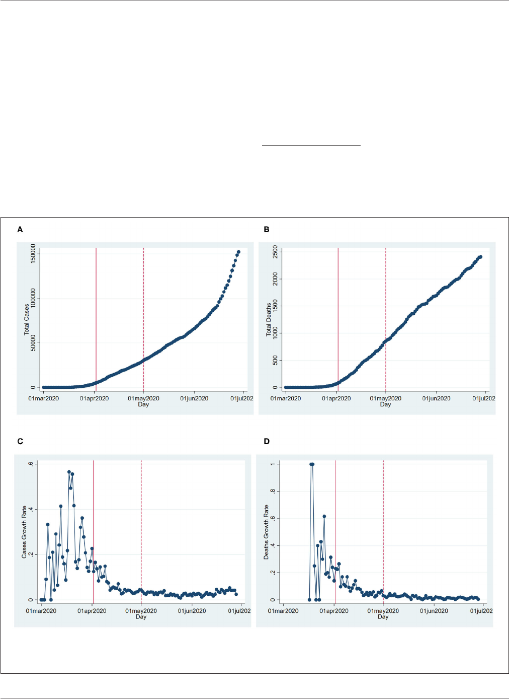
FIGURE 1 | COVID-19 cases and fatalities in Texas. (A) Cumulative cases. (B) Cumulative fatalities. (C) Daily cases growth. (D) Daily fatalities growth. This ﬁgure

shows the cumulative cases and fatalities, as well as their growth rates over the time in Texas. The solid and dashed vertical lines show the beginning (April 2, 2020)

and the end of the state-wide shelter-in-place order (May 1, 2020).

Frontiers in Public Health | www.frontiersin.org 3 November 2020 | Volume 8 | Article 596607

Castaneda and Saygili State-Wide Shelter-in-Place Order and Social Distancing in Texas

eﬀect. The model also includes a linear daily time trend. In

addition, we estimate the eﬀects of the SIPO on the growth rate of

cases and fatalities controlling for social distancing to determine

whether the policy had any eﬀects other than its eﬀect through

social distancing.

2.2.3. County-Level Analysis

The state-level analysis indicates that the SIPO reduced the

spread of the disease through its eﬀe ct on social distancing (the

percentage of the population sheltering in place). Therefore, we

use the county-level analysis to further investigate the eﬀect of

the statewide SIPO on social distancing, while controlling for

local policies.

First, we investigate th e eﬀect of the statewide SIPO on the

larger counties which implemented local policies before the

statewide SIPO (Harris, Dallas, Tarrant, Bexar, or Travis). In each

of these counties, ﬁrst, a public health emergency is declared,

which is then followed by a local stay-at-home order, and t hi s

is later followed by the state-wide shelter-in-place order. We

assume each policy replaces the former. For the analysis, we

estimated the following equation:

i,t

= β

+ α

SIPO

+ α

SIPO

+ α

SIPO

+ α

SIPO

+ β

i,t

+ θ

Day + u

(6)

where y

i,t

is the sheltering percentages in county i on day t and

i,t

includes the county-level policies (local emergency or local

shelter-in-place order). In addition, we control for a daily time

trend and county ﬁxed eﬀects. The regressions are weighted by

county-population and the standard errors are clustered at the

county-level.

Next, we investigate the eﬀect of the statewide SIPO on the

counties that never had any type of local county-level policy. If

the statewide SIPO is eﬀective in increasing the percentage of the

population that stays at home, one would expect counties without

any restrictive local policies to catch up with other counties

once the state-wide blanket policy is imposed. Therefore, we

estimated the following equation including all the counties in

the state:

i,t

= β

+ α

SIPO

+ α

SIPO

+ α

SIPO

+ α

SIPO

∗

NoPolicy + α

SIPO

∗

NoPolicy + α

SIPO

∗

NoPolicy+

SIPO

∗

NoPolicy + Day

+ u

i,t

(7)

where y

i,t

is the sheltering percentages in county i on day t. The

key variable, NoPolicy, i s a dummy that takes the value of one if

the county did not have any local policy prior to the statewide

SIPO. We include day and county ﬁxed-eﬀects. The regressions

are weighted by county population and the standard errors are

clustered at the county-level.

3. RESULTS

3.1. State-Level Results

Figure 1 shows the total cases and fat alit ies by day in Texas as

well as the growth rates of those. We estimate Equation (5) for

TABLE 1 | The growth of COVID-19 cases and fatalities.

Cases Fatalities

SIPO

−0.035 −0.067

(0.023) (0.061)

SIPO

−0.070*** −0.105**

(0.022) (0.051)

SIPO

−0.084*** −0.131***

(0.016) (0.043)

SIPO

−0.074*** −0.108***

(0.013) (0.036)

Day −0.002*** −0.004***

(0.000) (0.001)

Observations 117 102

Adjusted R

0.390 0.368

***,**Indicate signiﬁcance at 1% and 5%, respectively. Robust standard errors are reported

in parentheses.

the growth rate of cases and fatalities. The results in Table 1

show that the growth rates of cases are 0.07–0 .084 points lower

during the SIPO period. Given that the mean growth rate of

cases is about 0.1 outside the period, these numbers imply large

drops in the growth rates of cases during the period. Similarly,

the growth rate of deaths is 0.105–0.131 points lower during

the SIPO, t he largest decreases happening in the third week of

the policy.

We also analyze the impact of the policy on social distancing

measures. In particular, we look at the percentage of population

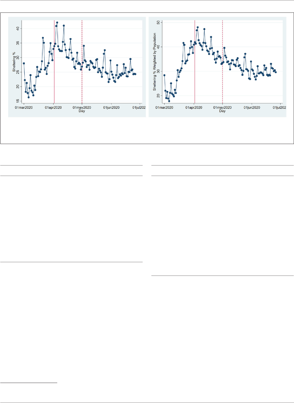
sheltering in place cre ated by SafeGraph. Figure 2 shows the

percentage of the population that shelters in place. Table 2

reports t h e regression results we get from estimating Equation

(5) for the sheltering percentages

. Both the table and ﬁgure

indicate the percentage of the population that shelters in

place is, on average, higher during the SIPO period. The

highest rate of sheltering corresponds to the ﬁrst week of

the SIPO, and the sheltering percentage gradually goes down

even when the SIPO was still in eﬀect. Compared to the

sheltering percentage outside the policy period (25%), the share

of sheltering population is about 9–41% higher during the

SIPO period.

Table 3 shows the impact of t he SIPO on the growth of

cases and fatalities when we control for lagged sheltering

percentages. Because of t he nature of the disease, social

distancing measures show impact only after a while. We estimate

Equation (5) using the 14-day lagged sheltering percentages in

addition to the SIPO indicators and time trends

. The table

reveals t hat the SIPO dummies are statistically insigniﬁcant

once the sheltering population is controlled for. These results

suggest the SIPO may slow down the spread of the disease

Weather conditions also aﬀect the sheltering percentages. More people are likely

to stay at home during rainy or cold days than on sunny days. However, we are

mainly interested in t he eﬀect of the SIPO on sheltering. As long as the weather

is not correlated with the enactment of the policy, our estimates would still be

unbiased (

18).

The ﬁt of the regression (R

) is largest with 13–15 days lags, and we use 14 days.

Frontiers in Public Health | www.frontiersin.org 4 November 2020 | Volume 8 | Article 596607

Castaneda and Saygili State-Wide Shelter-in-Place Order and Social Distancing in Texas

FIGURE 2 | Sheltering population. (A) Sheltering %. (B) Sheltering % weighted by population. This ﬁgure shows the average percentage of the population that stays

at home in Texas over time. The solid and dashed vertical lines show the beginning (April 2, 2020) and the end of the statewide shelter-in-place order (May 1, 2020).

For the right panel, the counties’ sheltering percentages are weighted by the counties’ populations, and then aggregated at the state level.

TABLE 2 | Sheltering population and the SIPO.

Sheltering %

SIPO

10.443***

(1.591)

SIPO

8.584***

(1.411)

SIPO

5.870***

(1.067)

SIPO

2.287***

(0.784)

Day 0.010

(0.013)

Observations 118

Adjusted R

0.400

***, **Indicate signiﬁcance at 1% and 5%, respectively. Robust standard errors are reported

in parentheses.

through its eﬀect on the percent age of people sheltering in

place. The policy itself is not signiﬁca nt once we control for

this percentage.

The state-level analysis shows one thing is clear: Social

distancing slows down the growth of cases

. The important

question remaining is whether the state-wide SIPO had a causal

impact on social dist ancing as measured by shelter-in-place

percentages. We address this question in th e next section.

3.2. County-Level Results

Figure 2 shows that the shelter-in-place percentages started

to increase well before t h e state-level SIPO order. According

to NACo, many counties adopted local policies such as

The Appendix shows we get similar results with county-level panel data.

TABLE 3 | The growth rates controlling for lagged sheltering percentages.

Cases Fatalities

SIPO

0.017 −0.018

(0.025) (0.051)

SIPO

−0.006 −0.043

(0.020) (0.033)

SIPO

0.020 −0.025

(0.027) (0.026)

SIPO

0.006 −0.027

(0.021) (0.021)

Lagged sheltering −0.009*** −0.009**

(0.002) (0.004)

Day −0.002*** −0.003***

(0.000) (0.001)

Observations 118 102

Adjusted R

0.442 0.409

***,**Indicate signiﬁcance at 1% and 5%, respectively. Robust standard errors are reported

in parentheses.

public health emergency and safer-at-home declarations days

or weeks before the state-wide policy. Overall, 70 counties

in Texas have at least one type of policy, emergency or

county-level shelter-in-place order, while 30 have both. The

adoption of these policies is unlikely to be random. In

particular, the size of the population and the number of

cases are positively correlated with the likelihood of restrictive

policies. This is particularly true for county-level stay-at-home

orders. Several counties declared a health emergency early

on when the cases were few. As the cases went up, the

counties with higher numbers of cases adopted shelter-in-

place orders.

Frontiers in Public Health | www.frontiersin.org 5 November 2020 | Volume 8 | Article 596607

Castaneda and Saygili State-Wide Shelter-in-Place Order and Social Distancing in Texas

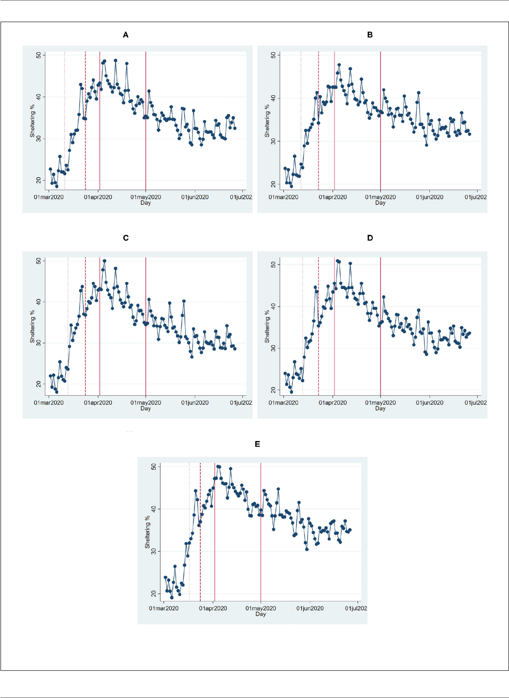
FIGURE 3 | Sheltering percentages in Texas counties. (A) Harris. (B) Dallas. (C) Tarrant. (D) Bexar. (E) Travis. This ﬁgure shows the percentage of the population that

stays at home in the ﬁve most populated counties of Texas over time. The dotted line shows the emergency declaration date, the dashed line shows the county-wide

SIPO, the solid lines mark the beginning and the end of the statewide SIPO.

Frontiers in Public Health | www.frontiersin.org 6 November 2020 | Volume 8 | Article 596607

Castaneda and Saygili State-Wide Shelter-in-Place Order and Social Distancing in Texas

We take a close look at the county-level trends in the most

populated ﬁve counties: Harris, Dallas, Tarrant, Bexar, and Travis.

These span the majority of the four biggest cities in Texas:

Houston (Harris), Dallas (Dallas and Tarrant), San Antonio

(Bexar), and Austin (Travis). These ﬁve counties make about 44%

of the total Texas population, while t h e remaining 249 counties

make up the rest. Perhaps not surprisingly, the earliest COVID-

19 cases emerged in t hese ﬁve counties. And, all of these counties

ordered a county-level stay-at-home policy before the state-wide

TABLE 4 | Sheltering percentages in most-populated Texas counties.

Sheltering % Sheltering % Sheltering %

Emergency 6.439***

(0.765)

County SIPO 10.724*** 12.998***

(0.417) (0.503)

SIPO

13.122*** 15.093*** 17.095***

(0.430) (0.442) (0.495)

SIPO

10.839*** 12.604*** 14.373***

(0.413) (0.426) (0.467)

SIPO

8.690*** 10.250*** 11.787***

(0.414) (0.427) (0.453)

SIPO

4.938*** 6.278*** 7.566***

(0.382) (0.396) (0.412)

Day 0.034*** 0.063*** 0.097***

(0.006) (0.006) (0.004)

Observations 585 585 585

Adjusted R

0.414 0.590 0.647

***, **Indicate signiﬁcance at 1% and 5%, respectively. Robust standard errors are reported

in parentheses.

SIPO. They also declared a county-wide emergency even before

the sheltering policies

Figure 3 shows the percentage of the populations sheltering

in place in each of these counties. Table 4 shows the

results from estimating Equation (6). The results reveal that

the initial pronounced increase in sheltering percentages

corresponds to the declaration of county-wide emergency and

shelter-in-place orders.

Next, we take a look at the counties that never had any type

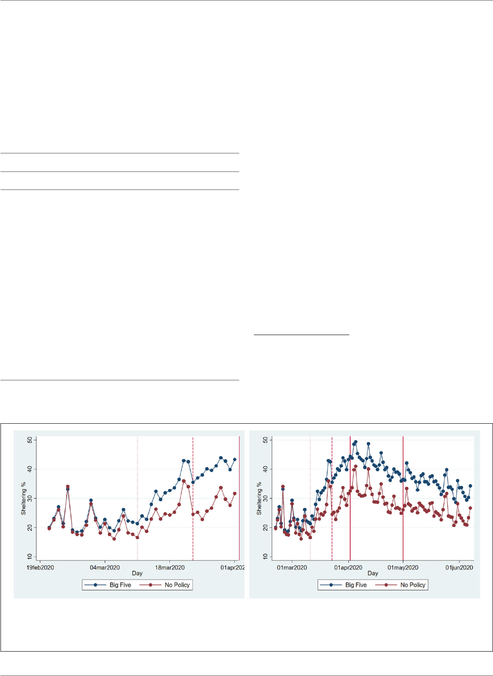
of county-level policy. Figure 4 shows that there is a signiﬁcant

diﬀerence in terms of sheltering population in the biggest ﬁve

counties vs. counties that never adopted any type of policy prior

to the state-wide SIPO. The panel that shows the trends before the

state SIPO revea ls that in both groups of counties, the sheltering

percentage increases over time. However, t he gap widens over

time. Interestingly, even after the implementation of the state

SIPO, the gap persisted. The policy did not disproportionately

aﬀect the counties with no prior policies. Also, the gap carries

on after the SIPO expires. The ﬁgure suggests that more people

shelter in highly populated areas. This may still be a reﬂection of

the fact that the perceived risk of catching t he disease is higher in

those areas, and the impact of fear is strong enough to keep more

people at home.

If the SIPO is eﬀective in increasing t he percentage of the

population that stays at home, one would expect counties without

any restrictive policies to catch up wit h others once the state-wide

blanket policy is imposed. We estimate Equation (7) including

Harris county declared public health emergency on March 11, and stay at home

order on March 24, which is 9 days prior to the state-wide policy. Similarly, Dallas

county declared an emergency on March 12 and ordered residents to stay at home

on March 23. Tarrant county’s emergency declaration is on March 13, and the

county-level SIPO date is March 24. Bexar county’s declarations were on March 13

and March 23, respectively. For Travis county, the dates are March 17 and March

24, respectively.

FIGURE 4 | Sheltering percentages. (A) Before SIPO. (B) Whole period. The ﬁgure shows the average sheltering percentages in two groups of counties: The most

populated ﬁve (Harris, Dallas, Tarrant, Bexar, and Travis) and the counties that never adopted any county-level policy. The dotted line shows the earliest emergency

declaration date among the largest ﬁve (March 11, 2020), the dashed line shows the earliest county-wide SIPO (March 23, 2020), the solid lines mark the beginning

and the end of the statewide SIPO.

Frontiers in Public Health | www.frontiersin.org 7 November 2020 | Volume 8 | Article 596607

Castaneda and Saygili State-Wide Shelter-in-Place Order and Social Distancing in Texas

TABLE 5 | Sheltering percentages all Texas counties.

Sheltering % Sheltering % Sheltering %

SIPO

18.729*** 19.075*** 20.241***

(0.679) (0.672) (0.644)

SIPO

16.474*** 16.798*** 18.017***

(0.687) (0.673) (0.635)

SIPO

15.548*** 15.946*** 16.886***

(0.628) (0.612) (0.634)

SIPO

10.963*** 11.341*** 12.299***

(0.613) (0.577) (0.550)

SIPO

*NoPolicy −1.855*** −8.093***

(0.563) (1.066)

SIPO

*NoPolicy −1.736*** −8.257***

(0.542) (1.084)

SIPO

*NoPolicy −2.131*** −7.158***

(0.472) (1.010)

SIPO

*NoPolicy −2.021*** −7.144***

(0.424) (0.929)

Fixed effects

County Yes Yes Yes

Day Yes Yes Yes

Day-NoPolicy No No Yes

Observations 29,718 29,718 29,718

Adjusted R

0.934 0.936 0.945

***,**,*Indicate signiﬁcance at 1, 5, and 10%, respectively. Robust standard errors are

reported in parentheses.

all of the 254 counties. The results in Table 5 shows that the

sheltering percentage is highest in the ﬁrst week of the SIPO

and gradually decreases, conﬁrming our earlier results. However,

there is no evidence that the sheltering percentage in the counties

without any prior policy converges to the percentages in the

counties with proactive policies. In contrast, there seems to be

a gap between these groups of counties, which persists during the

policy period.

4. CONCLUSION AND DISCUSSION

We analyze both state and c ounty-level eﬀe ct s of the SIPO on the

growth of cases and deaths. We ﬁnd t hat growth and death rates

are lower during the SIPO period. We also see that a signiﬁcantly

larger percentage of the population stays at home during this

period. Thus, it is not surprising to see that the disease slows

down in the period of the SIPO. The more interesting question

is whet h er the SIPO caused stay a t home percentages to increase.

We ﬁnd two pieces of evidence that goes against such causality.

First, even though the highest sheltering corresponds to the ﬁrst

week of the SIPO, sheltering percentages steadily declined even

though the policy was in eﬀect (Figures 2, 3). This pattern might

be very much a behavioral response to the emergence and the

initial rapid spread of the disease. The fact that people start to see

cases in their communities may create fear, and people respond

by staying at home. However, as the duration of home stay gets

longer, people might develop fatigue and start moving again.

Second, we make use of the fact that some counties adopted local

“safer at home” policies several days before the state-wide blanket

policy. The sheltering percentages in these counties started to

increase before the state-wide SIPO. However, we see a similar

upward trend, albeit at a slower rate, in counties where there

were no such policies. Also, we do not observe that these groups

of counties converge to a similar sheltering percentage after

the state-wide blanket policy. Instead, the counties without any

policy (less populated counties with slower growt h of cases) have

a lower rate of sheltering than the other counties. There seems to

be a gap in terms of sheltering percentages, and it persists during

as well as after the policy period (Figure 4).

Our analyses show that the growth rate of COVID-19 cases

and deaths decreases when a larger share of the population

exercises social distancing by staying at home. However, we

do not ﬁnd evidence that the state-wide shelter-in-place order

increased the percentage of the population that stay s at home.

The initial local conditions and county policies may have already

encouraged people to stay at home. It may be a better strategy

to reach out to the population and inform them about the

current state of disease in their localities. On the other hand,

policymakers also need to consider the fact that people may not

be able to stay at home even if they want to if their employers ask

them to get back to work in the absence of such policies. What

we suggest is that imposing restrictive policies alone may not be

enough to guarantee that people will exercise soci al distancing.

Thus, such policies must take local conditions into account and

be accompanied by the eﬀort to inform and educate the public

about the potential consequences of the disease and the situation

in t hei r communities.

Even though the current study has interesting policy

implications, it has limita tions. In particular, the results may not

need to generalize to other states or countries. A similar evolution

of the pandemic and similar policy rules may generate quite

diﬀerent behavioral responses from the public elsewhere. More

local-level studies may be needed to check the generalizability of

our conclusions.

DATA AVAILABILITY STATEMENT

Publicly available datasets were analyzed in this study. This data

can be found here: https://covid19.unfolded.ai/, https://www.

naco.org/covid19/topic/research- data.

AUTHOR CONTRIBUTIONS

All authors listed have made a substantial, direct and

intellectual contribution to the work, and approved it

for publicati on.

Frontiers in Public Health | www.frontiersin.org 8 November 2020 | Volume 8 | Article 596607

Castaneda and Saygili State-Wide Shelter-in-Place Order and Social Distancing in Texas

REFERENCES

1. Saglietto A, D’Ascenzo F, Zoccai GB, De Ferrari GM. COVID-

19 in Europe: the Italian lesson. Lancet. (2020) 395:P1110–1.

doi: 10.1016/S0140-6736(20)30690-5

2. Yuan J, Li M, Lv G, Lu ZK. Monitoring transmissibility and

mortality of COVID-19 in Europe. Int J Infect Dis. (2020) 95:311–5.

doi: 10.1016/j.ijid.2020.03.050

3. Dave D, Friedson AI, Matsuzawa K, Sabia JJ. When do shelter-in-place orders

ﬁght COVID-19 best? Policy heterogeneity across states and adoption time.

Econ Inq. (2020). doi: 10.1111/ecin.12944. [Epub ahead of print].

4. Killgore WDS, Cloonan SA, Taylor, EC, Dailey NS. Loneliness: a signature

mental health concern in the era of COVID-19. Psychiatry Res. (2020)

290:113117. doi: 10.1016/j.psychres.2020.113117

5. Smith ML, Steinman LE, Casey EA. Combatting social isolation among older

adults in a time of physical distancing: the COVID-19 social connectivity

paradox. Front. Public Health. (2020) 8:403. doi: 10.3389/fpubh.2020.

00403

6. Bhutani S, Cooper JA. COVID-19-related home conﬁnement in

adults: weight gain risks and opportunities. Obesity. (2020) 28:1576–7.

doi: 10.1002/oby.22904

7. Stoker S, McDaniel D, Crean T, Maddox J, Jawanda G, Krentz N, et al. Eﬀect of

shelter-in-place orders and the COVID-19 pandemic on orthopaedic trauma

at a community level II trauma center. J Orthop Trauma. (2020) 34:e336–42.

doi: 10.1097/BOT.0000000000001860

8. Bullinger LR, Carr JB, Packham A. “COVID-19 and crime: eﬀects of stay-

at-home orders on domestic violence,” in NBER Working Paper 27667.

Cambridge, MA (2020).

9. Froimson JR, Bryan DS, Bryan AF, Zakrison TL. COVID-19,

home conﬁnement, and the fallacy of “safest at home”. Am

J Public Health. (2020) 110:960–1. doi: 10.2105/AJPH.2020.

305725

10. Kofman YB, Garﬁn DR. Home is not always a Haven; The domestic violence

crisis amid the COVID-19 pandemic. Psychol Trauma Theory Res Pract Policy.

(2020) 12:S199–201. doi: 10.1037/tra0000866

11. Sen S, Karaca-Mandic P, Georgiou A. Association of stay-at-home orders

with COVID-19 hospitalizations in 4 states. JAMA. (2020) 323:2522

U-4.

doi: 10.1001/jama.2020.9176

12. Wei L, Wehby GL. Shelter-in-Place orders reduced COVID-19 mortality and

reduced the rate of growth in hospitalizations. Health Aﬀ. (2020) 39:1615–23.

doi: 10.1377/hlthaﬀ.2020.00719

13. Courtemanche C, Garuccio K, Le A, Pinkston J, Yelowitz A. Strong social

distancing measures in the United States reduced the COVID-19 growth rate.

Health Aﬀairs. (2020) 39:1237 –4 6. doi: 10.1377/hlthaﬀ.2020.00608

14. Friedson AI, McNichols D, Sabia JJ, Dave D. “Did California’s shelter-in-

place order work? Early Coronavirus-related public health eﬀects,” in NBER

Working paper 26992. Cambridge, MA (2020). Available online at: https://

onlinelibrary.wiley.com/doi/abs/10.1111/ecin.12944

15. Ashby NJS. Impact of the COVID-19 pandemic on unhealthy eating in

populations with obesity. Obesity. (2020) 28:1802–5. doi: 10.1002/oby.22940

16. Weill JA, Stigler M, Deschenes O, Springborn MR. S ocial distancing responses

to COVID-19 emergency declarations strongly diﬀerentiated by income. Proc

Natl Acad Sci USA. (2020) 117:19658–60. doi: 10.1073/pnas.2009412117

17. Woody S, G arcia Tec M, Dahan M, Gaither K, Lachmann M, Fox S,

et al. Projections for ﬁrst-wave COVID-19 deaths across the US using

social-distancing measures derived from mobile phones. medRxiv. (2020).

doi: 10.1101/2020.04.16.20068163

18. Wooldridge JM. Introductory Econometrics: A Modern Approach. 6th ed.

Cengage Learning (2016).

Conﬂict of Interest: The authors declare that the research was conducted in the

absence of any commercial or ﬁnancial relationships that could be construed as a

potential conﬂict of interest.

under the terms of the Creative Commons Attribution License (CC BY). The use,

distribution or reproduction in other forums is permitted, provided the original

author(s) and the copyright owner(s) are credited and that the original publication

in this journal is cited, in accordance with accepted academic practice. No use,

distribution or reproduction is permitted which does not comply with these terms.

Frontiers in Public Health | www.frontiersin.org 9 November 2020 | Volume 8 | Article 596607

Castaneda and Saygili State-Wide Shelter-in-Place Order and Social Distancing in Texas

APPENDIX

Including all of the 254 Texas counties, we estimate the

following regression:

i,t

= β

+ α

SIPO

+ α

SIPO

+ α

SIPO

+ α

SIPO

+ Time

+ County

+ u

i,t

(A1)

where y

i,t

is the growth rate of cases and fatalities in county i

at time t. We control for time and county ﬁxed eﬀects, and we

cluster standard errors at the county-level. All estimations are

weighted by county population.

Time captures days after the ﬁrst case rather than c alend a r

days. This way, we are comparing counties at the same point in

the evolution of t h e disease’s spread. If the spread of the disease

were strictly exponential, this choice would not matter since the

growth rate of cases would be the same regardless of whether

a county has a few cases or many c ases. Since we know the

strict exponentiality is not realistic, our choice provides better

estimates. The results in Table A1 shows that the growth rate of

cases is 0.053–0.079 points lower during the SIPO period. The

growth rates of fatalities are 0.032–0.058 point lower.

Next, we look at the relation between the percentage of the

population that stays at home in each county and the state-wide

shelter-in-place order. We estimate Equation (A1) where y

i,t

the percentage of sheltering population. We control for county

and time ﬁxed-eﬀe cts, cluster standard errors at the county level,

and weight regressions by the counties’ populations. The ﬁrst

column in Table A2 shows that the sheltering is 12.4 percentage

points (almost 50%) higher in the ﬁrst of the SIPO period. Even

though the sheltering percentages are statistically larger in the

following weeks as well, the margin decreases gradually. We

also include dummies for 1 and 2 weeks before the SIPO to see

how sheltering percentages look before the policy. The last two

column reveals that the upward trend in sheltering percentages

started even before the policy.

TABLE A1 | The growth of COVID 19 cases and fatalities.

Cases Fatalities

SIPO

−0.053*** 0.014

(0.014) (0.041)

SIPO

−0.075*** −0.045***

(0.013) (0.015)

SIPO

−0.079*** −0.058***

(0.011) (0.015)

SIPO

−0.054*** −0.032***

(0.007) (0.010)

Fixed effects

County Yes Yes

Time Yes Yes

Observations 19,343 8,231

Adjusted R

0.353 0.151

***,**Indicate signiﬁcance at 1, 5, and 10%, respectively. Robust standard errors are

reported in parentheses.

TABLE A2 | Sheltering percentages and the SIPO.

Sheltering % Sheltering % Sheltering %

SIPO

-2

6.061***

(0.879)

SIPO

-1

12.542*** 12.542***

(0.597) (0.597)

SIPO

12.397*** 12.397*** 12.397***

(0.635) (0.635) (0.635)

SIPO

10.142*** 10.142*** 10.142***

(0.649) (0.649) (0.649)

SIPO

9.217*** 9.217*** 9.217***

(0.614) (0.614) (0.614)

SIPO

4.632*** 4.632*** 4.632***

(0.591) (0.591) (0.591)

Fixed effects

County Yes Yes Yes

Time Yes Yes Yes

Observations 29,972 29,972 29,972

Adjusted R

0.933 0.933 0.933

***,**Indicate signiﬁcance at 1% and 5%, respectively. Robust standard errors are reported

in parentheses.

TABLE A3 | The Growth rates controlling for lagged sheltering percentages.

Cases Fatalities

SIPO

−0.012 0.038

(0.010) (0.036)

SIPO

−0.014 −0.014

(0.012) (0.014)

SIPO

0.003 −0.019

(0.011) (0.014)

SIPO

0.001 −0.006

(0.008) (0.009)

Lagged sheltering −0.007*** −0.004**

(0.001) (0.001)

Fixed effects

County Yes Yes

Time Yes Yes

Observations 19,286 8,231

Adjusted R

0.403 0.155

***,**Indicate signiﬁcance at 1% and 5%, respectively. Robust standard errors are reported

in parentheses.

The SIPO is expected to slow down the spread of the

disease by increasing social dista ncing in the population.

So, we expect it to inﬂuence the spread of disease via its

eﬀect on the number of people sheltering in place. Due to

the nature of the disease, a change in sheltering behavior

impacts the spread of the disease with a lag. We estimate

Frontiers in Public Health | www.frontiersin.org 10 November 2020 | Volume 8 | Article 596607

Castaneda and Saygili State-Wide Shelter-in-Place Order and Social Distancing in Texas

Equation (A1) controlling for the sheltering percentage

14 days prior. The independent variable y

i,t

is th e growth

rate of cases or deaths. We include county and time

dummies, and weigh regressions by county populations.

Table A3 shows past sheltering percentages are statistically

signiﬁcant determinants of the current growt h of cases

and fatalities, while the SIPO dummies are no longer

statistically signiﬁcant.

Frontiers in Public Health | www.frontiersin.org 11 November 2020 | Volume 8 | Article 596607