
DISCUSSION PAPER SERIES
IZA DP No. 13262
Dhaval Dave
Andrew Friedson
Kyutaro Matsuzawa
Joseph J. Sabia
Samuel Safford
Were Urban Cowboys Enough to Control
COVID-19?
Local Shelter-In-Place Orders and
Coronavirus Case Growth
MAY 2020
Any opinions expressed in this paper are those of the author(s) and not those of IZA. Research published in this series may
include views on policy, but IZA takes no institutional policy positions. The IZA research network is committed to the IZA
Guiding Principles of Research Integrity.
The IZA Institute of Labor Economics is an independent economic research institute that conducts research in labor economics
and offers evidence-based policy advice on labor market issues. Supported by the Deutsche Post Foundation, IZA runs the
world’s largest network of economists, whose research aims to provide answers to the global labor market challenges of our
time. Our key objective is to build bridges between academic research, policymakers and society.
IZA Discussion Papers often represent preliminary work and are circulated to encourage discussion. Citation of such a paper
should account for its provisional character. A revised version may be available directly from the author.
Schaumburg-Lippe-Straße 5–9
53113 Bonn, Germany
Phone: +49-228-3894-0
IZA – Institute of Labor Economics
DISCUSSION PAPER SERIES
ISSN: 2365-9793
IZA DP No. 13262
Were Urban Cowboys Enough to Control
COVID-19?
Local Shelter-In-Place Orders and
Coronavirus Case Growth
MAY 2020
Dhaval Dave
Bentley University, IZA and NBER
Andrew Friedson
University of Colorado Denver
Kyutaro Matsuzawa
San Diego State University
Joseph J. Sabia
San Diego State University and IZA
Samuel Safford
San Diego State University

ABSTRACT
IZA DP No. 13262 MAY 2020
Were Urban Cowboys Enough to Control
COVID-19?
Local Shelter-In-Place Orders and
Coronavirus Case Growth
*
One of the most common policy prescriptions to reduce the spread of COVID-19 has been
to legally enforce social distancing through state or local shelter-in-place orders (SIPOs). This
paper is the first to explore the comparative effectiveness of early county-level SIPOs versus
later statewide mandates in curbing COVID-19 growth. We exploit the unique laboratory
of Texas, a state in which the early adoption of local SIPOs by densely populated counties
covered almost two-thirds of the state’s population prior to Texas’s adoption of a statewide
SIPO on April 2, 2020. Using an event study framework, we document that countywide
SIPO adoption is associated with a 14 percent increase in the percent of residents who
remain at home full-time, a social distancing effect that is largest in urbanized and densely
populated counties. Then, we find that in early adopting counties, COVID-19 case growth
fell by 19 to 26 percentage points two-and-a-half weeks following adoption, a result robust
to controls for county-level heterogeneity in outbreak timing, coronavirus testing, and
border SIPO policies. This effect is driven nearly entirely by highly urbanized and densely
populated counties. In total, we find that approximately 90 percent of the curbed growth
in statewide COVID-19 cases in Texas came from the early adoption of SIPOs by urbanized
counties. These results suggest that the later statewide mandate yielded relatively few
health benefits.
JEL Classification: H75, I18
Keywords: coronavirus, shelter-in-place orders, COVID-19, urbanicity,
population density
Corresponding author:
Joseph J. Sabia
Department of Economics
San Diego State University
5500 Campanile Drive
San Diego, CA 92182-4485 USA
E-mail: [email protected]
* Sabia acknowledges research support from the Center for Health Economics & Policy Studies at San Diego State
University, including grant funding received from the Charles Koch Foundation and Troesh Family Foundation.

1
1. Motivation
The first case of COVID-19 in the United States was confirmed on January 20, 2020 in
Washington State (Holshue et al. 2020). The disease rapidly spread among the U.S. population
over the following months, with the U.S. becoming the country with the most confirmed cases of
COVID-19 on March 26, 2020 (Johns Hopkins University 2020). As of May 1, 2020, COVID-
19 was confirmed to have killed over 59 thousand Americans, surpassing the American death toll
due to the Vietnam War (Defense Casualty Analysis System 2008; Johns Hopkins University
2020).
Public health responses to the COVID-19 pandemic have centered around a variety of
non-pharmaceutical interventions (NPIs) such as closing schools, closing restaurants and other
businesses, banning larger gatherings, and issuing blanket shelter-in-place orders (SIPOs).
While the federal government has the ability to make disaster declarations, offer public health
recommendations, and direct resources (for example, the federal government can force industries
to produce needed medical supplies under the Defense Production Act), the power to enact most
NPIs rests with state and local governments.
The efficacy of NPIs at slowing the spread of COVID-19 is the subject of a growing
literature. National studies such as Dave et al. (2020) and Courtemanche et al. (2020a), as well
as studies of state-specific policy interventions in California (Friedson et al. 2020) and in
Kentucky (Courtemanche et al. 2020b) have shown sizable reductions in the growth rate of
COVID-19 cases due to certain NPIs, in particular SIPOs.
1
1
Courtemanche et al. (2020a) and Courtemanche et al. (2020b) found no improvement in case growth rates from
school closures or bans on large gatherings, modest improvements from restaurant and entertainment center closures
and large improvements from SIPOs. Friedson et al. (2020) and Dave et al. (2020) documented large improvements
from SIPOs.
2
SIPOs carry legal penalties for failure to comply with “social distancing” behavior, i.e.
maintaining physical distance from individuals outside of one’s household (Allday 2020). Social
distancing is a primary recommendation for slowing the spread of COVID-19 from the Centers
for Disease Control and Prevention along with other contagion-reducing activities such as hand
washing and wearing face coverings in public (Centers for Disease Control 2020). SIPOs have
been empirically demonstrated to improve social distancing by reducing the frequency that
individuals travel outside of their homes using anonymized cell phone location data (Dave et al.
2020; Friedson et al. 2020).
As COVID-19 is a disease that is spread via close proximity to others, and can be spread
by asymptomatic individuals (Bai et al. 2020; Pan et al. 2020; Rothe et al. 2020), the speed at
which the disease spreads in the absence of intervention will depend on how frequently
individuals come in close contact. Thus, the speed of transmission in a given location will be in
part a function of how densely populated a location is. This means that SIPOs (and other NPIs)
could vary greatly in their efficacy based on the density of the local population. Indeed, Dave et
al. (2020) showed that SIPOs were much more effective at slowing the spread of COVID-19 in
states that had higher average population density relative to states with lower average population
density.
State level population density, however, does not capture the large amount of variation in
population density across locations within a state. In 2010, metropolitan statistical areas had an
average population density of 282.9 persons per square mile, whereas micropolitan statistical
areas had an average population density of 82.5 persons per square mile, and locations outside of
core-based statistical areas (i.e. rural locations) had an average population density of 42.0
persons per square mile (Wilson et al. 2012). Thus, blanket NPIs that uniformly cover a variety

3
of locations within a single state could have significant variation in their ability to slow the
spread of disease.
This leads to an important policy question: is it possible to judiciously apply local SIPOs
only in more densely populated locations, and still receive the majority of their public health
benefits without a blanket statewide order across heterogeneously populated jurisdictions?
Given that SIPOs may have important job-related costs (Baek et al. 2020), understanding how to
achieve public health benefits at the least cost is important.
In order to empirically answer this question, it is necessary to narrow to a within-state
analysis, capitalizing on natural experiments occurring within states that enacted statewide
SIPOs, but also had a substantial number of localities enacting local orders prior to the state
SIPO. Moreover, given the incubation period of COVID-19 of approximately 5-12 days (Lauer
et al. 2020), a sufficiently lengthy time window is needed between when the earliest localities
enacted their orders and the later statewide order, to disentangle the effects of each. Our focus
on the roles of population density and urbanicity in potentially reinforcing the effects of social
distancing measures also requires that early local orders are adopted across a slate of urbanized,
non-urbanized, populated, and sparse counties.
These considerations direct our main analysis to the state of Texas, which has a number
of features that make it an ideal laboratory for studying the efficacy of SIPOs based on
population density. Texas enacted a statewide SIPO, but did so quite late relative to other states.
California, which enacted the first statewide SIPO, did so on March 19th, whereas Texas enacted
its statewide SIPO on April 2nd, the 34th state to do so.
2
However, 85 of Texas’ 254 counties
enacted their own county-level SIPOs prior to the statewide order, with 34 of the county orders
2
Texas is tied with Maine as the 34
th
state to enact a statewide SIPO.

4
enacted over a week prior to the statewide order – the most, by far, out of any other statewide
SIPO-enacting state. Of these 34 early-adopting counties, 18 had urbanicity rates (percentage of
population living in urbanized areas or urban clusters) of greater than 75 percent and 10 had
urbanicity rates of over 90 percent, both the highest among statewide SIPO states with early
adopting counties. Moreover, 18 of 34 early-adopting Texas counties had population densities
greater than 150 persons per square mile,
3
and 5 had population densities greater than 1,000
persons per square mile, each of which constituted the largest number of early-adopting counties
among statewide-SIPO adopting states.
Relatedly, in terms of coverage, Texas also had the greatest flurry of activity with respect
to the early local orders; these early local orders covered approximately two-thirds (66 percent)
of the state’s population a week prior to the statewide SIPO order, a share greater than any other
state. Thus, these county SIPO policies created important variation both in the timing of local
SIPOs as well as the density of the local population impacted by these local orders, both critical
in answering our research questions.
4
By leveraging these differences, as well as daily data on both social distancing behavior
(via anonymized cell phone location data) and COVID-19 cases, we demonstrate that (1) county-
level SIPOs enacted in Texas were somewhat more effective at eliciting social distancing
behavior in more densely population areas, and (2) county-level SIPOs in Texas were immensely
more effective at slowing the spread of the disease in more densely populated areas.
3
The 18 counties with population densities greater than 150 persons per square mile were not identical to the 18
counties with population densities greater than 150 persons per square mile. For example, among the “high
urbanicity” counties that were not classified as “high population density counties” (using the 150 persons per square
population cutoff) were Hood County, Starr County, Stephens County, Val Verde County, and Willacy County.
Those counties with more than 150 persons per population with urbanicity rates less than 75 percent were Ellis,
Hays, Hunt, Kaufman, and McLennan counties.
4
Texas provided the most jurisdiction-level variation with 34 counties enacting a local order at least 7 days prior to
the statewide order, more than double that of the state with the next most variation (Missouri), which covered less of
the state population than Texas.

5
These results have important implications for public health policies moving forward. As
policies such as SIPOs may have important economic costs associated with them (Baek et al.
2020), if government can move from one-size-fits-all policies, such as statewide SIPOs to more
nuanced policies based on the characteristics of each location, such as SIPOs targeted at more
densely populated areas, it may be possible to improve public welfare without making large
sacrifices to public health.
2. Data and Methods
2.1 Social Distancing Data
To measure county-level social distancing, we utilize data from SafeGraph, Inc.,
following Friedson et al. (2020) and Dave et al. (2020). These data are generated from 45
million anonymized GPS cell phone pings that can be used to measure the degree of social
distancing among a local population, in this case at the county level.
A cell phone’s “home” is defined as the 153- by 153-meter location where the cell phone
is pinged most frequently during the hours between 6pm and 7am. We then measure the percent
of the cell phones (and presumably residents who own said cell phones) within a county that
spend a given day within the “home” location. This margin of social distancing, measuring all-
day stay-at-home behavior, is not based on total distance traveled, and therefore also enables
better comparisons between rural and urban counties than other measures that can be calculated
with SafeGraph.
5
On March 18, 2020, about five days prior to the adoption of a SIPO in early-adopting
urban counties (as there is some variation in implementation dates between these counties), 31.8
5
It is still possible that there is a degree of undercounting in this measure for rural residences, as they are more
likely to be larger than 153- by 153-meters than urban residences.

6
percent of residents had stayed at home full-time, subsequently increasing to 41.2 percent (by 9.4
percentage points) by March 30. To contrast, five days prior to the statewide SIPO, 34.9 percent
of residents in counties that had not adopted a local SIPO — counties with an average urbanicity
rate under 20 percent — sheltered-in-place full-time. By five days following the statewide order,
37.6 percent did so (an increase of only 2.7 percentage points). This pattern of findings suggests
that local SIPOs may have had larger effects for early adopting urban counties relative to non-
adopting counties. We return to these findings below, where we test these relationships
formally.
2.2 COVID-19 and Policy Data
We draw county-level daily data on reported COVID-19 cases in Texas from March 8,
2020 through April 28, 2020 for our analyses. These data are compiled by county public health
departments, reported to the Centers for Disease Control and Prevention, and made public via the
Kaiser Family Foundation.
6
By April 28, 2020, there were a total of 1,012,878 confirmed
reported coronavirus cases in the United States, 26,865 (2.7 percent) of which were in the State
of Texas. Over the period from March 8 through April 28, there was an average of 34.5 new
cases per state-day.
7
Local policy data on SIPOs, as well as data on local non-essential business closures and
emergency decrees were collected by the Center for Health Economics & Policy Studies at San
Diego State University. As noted above, a shelter-in-place order (SIPO) is one of the most
6
These data can be obtained here: https://github.com/nytimes/covid-19-data
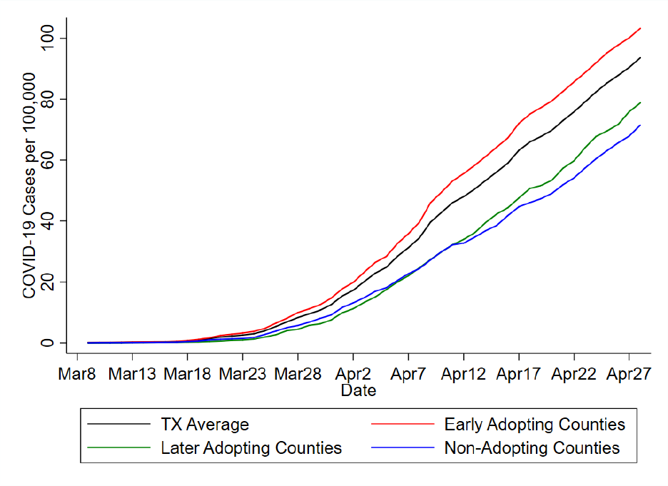
7
Over this period, there were a total of 53,034 COVID-19 deaths, 738 (1.4 percent) of which were in the State of
Texas. Appendix Figure 1 shows coronavirus case growth statewide for Texas over our sample window, and across
early adopting counties (which enacted a SIPO at least 7 days prior to the state order on April 2
nd
), later adopting
counties (that issued a SIPO prior to but within 6 days of the statewide order), and non-adopting counties (that were
bound by the statewide order).
7
restrictive emergency measures taken by a jurisdiction in order to combat a current emergency.
These orders require all local residents and visitors to stay-at-home or shelter-in-place for all but
essential activities. While there are a limited number of jurisdictions that issued SIPOs to
targeted populations (i.e. elderly, juveniles, recent international travelers), full SIPOs are
imposed on all present in a county or state. SIPOs are also accompanied by a full non-essential
business closure. Data on state and county SIPOs are collected using information compiled by
the National Association of Counties (2020), Mervosh et al. (2020), Friedson et al. (2020), and
our own searches of official county websites, county court records, local news agencies, and
gubernatorial executive orders and proclamations.
Data on non-essential business closures (NEBCOs) are also collected via searches of
official county governmental websites (county executive or legislative branches, including
county departments of health), county court records, local news agencies, and state records of
gubernatorial executive orders or proclamations. NEBCOs primarily serve to mandate the
closure of all businesses not deemed to be essential for day-to-day operations. Common essential
businesses regularly include grocery stores, gas stations, funeral homes, some healthcare
facilities, pharmacies, veterinarians, and financial institutions (including banks).
We also collect information on county emergency decrees through searches of official
county websites, county court records, local news agencies, and the National Association of
Counties (2020). These declarations are formal proclamations issued by a jurisdiction’s chief
public official (i.e. Mayors, County Judges, County Executives, or Governors) announcing that a
current or impending crisis will require additional action that exceeds a county or (state’s)
standard resource response capabilities. Such declarations typically include language invoking
emergency powers and operations for a pre-determined period of time, which can then be

8
extended if deemed necessary. These powers commonly include the authorization for a county to
request all assistance available from higher jurisdictions, as well as the activation of a local
Public Health or Emergency Management agency to take actions to protect the public health.
In addition, we collect data on average temperature in the county and whether there was
measurable precipitation in the county as weather conditions may on the margin influence
individual compliance with social distancing. These data are drawn from the National Centers for
Environmental Information at the National Oceanic and Atmospheric Administration.
8
Finally, we collect information on the urbanicity (the percent of a county’s population
that lives within urbanized areas or urban clusters) and population density of Texas counties
from the 2010 Census.
9
The median urbanicity rate of a Texas county was 46 percent and the
median population density rate was 22 persons per square mile.
2.3 Methods
The aim of this study is to assess whether public health effects accrued to local
jurisdictions adopting a shelter-in-place order early, in advance of the statewide order, and
whether any potential benefits were magnified in such early-adopting jurisdictions that had a
more tightly packed population. Our empirical analysis proceeds in a stepwise manner to address
these questions.
We begin by estimating the first-order relationship between county-level SIPO adoption
and social distancing through a difference-in-differences identification strategy:
8
These data are at: https://www.ncdc.noaa.gov/cdo-web/. Appendix Table 1 presents the sample means for all
variables.
9
This includes urbanized Areas (UAs) of 50,000 or more people or urban clusters of at least 2,500 and less than
50,000 people. These data are available at: https://www.census.gov/programs-surveys/geography/guidance/geo-
areas/urban-rural/2010-urban-rural.html
9
PCTHOME
ct
= γ
0
+ γ
1
SIPO
ct
+ X’
ct
β
2
+ α
c
+ τ
t
+ ε
ct
(1)
where PCTHOME
cs
measures the share of the county population that remained at home full-time,
SIPO
ct
is an indicator for whether a shelter-in-place order was in effect in county c on day t, and
X
ct
is a set of county-specific time-varying controls, including whether the county had issued an
emergency declaration, whether a non-essential business closure order had been enacted (but not
a SIPO), the average temperature in the county, and whether measurable precipitation fell in the
county. In addition, α
c
is a county fixed effect and τ
t
is a day fixed effect. This model, and all
models that follow, are weighted using the county population and utilize standard errors
corrected for clustering at the county-level (Bertrand et al. 2004).
We next explore whether the social distancing effects of SIPOs differ by whether the
county was more highly urbanized or more densely populated:
PCTHOME
ct
= γ
0
+ γ
1
SIPO
ct
*Urban
c
+ X
ct
β
2
+ α
c
+ τ
t
+ ε
ct
(2)
where Urban
c
identifies mutually exclusive indicators for whether the county urbanicity rate was
greater or less than 75 percent in the 2010 Census. Alternatively, we replace Urban
c
with
PopDensity
c
, an indicator for whether the county population density was greater than 150
persons per square mile in the 2010 Census. In Texas, 23.6 percent of all counties have
urbanicity rates of greater than 75 percent and 13.0 percent are classified as higher population
density using our definition.

10
Next, we examine the public health effects of local SIPO adoption by focusing on the
growth in COVID-19 cases, following Courtemanche et al. (2020a, b), and estimating the
following specification that accounts for (i) early SIPO adoption by counties, and (ii) lagged
effects of SIPOs:
COVID Growth
ct,t-1
= β
0
+ (SIPO 0 to 4 Days
ct
* Adopt
c
) β
1
+ (SIPO 5 to 8 Days
ct
* Adopt
c
) β
2
+ (SIPO 9 to 18 Days
ct
* Adopt
c
) β
3
+ (SIPO >18 Days
ct
* Adopt
c
) β
4
+ X’
ct
β
5
+ α
c
+ τ
t
+ ε
ct
(3)
where COVID Growth
ct,t-1
is the difference in the natural log of cumulative COVID-19 cases in
county c on day t and day t-1, and thus reflects new confirmed cases each day. SIPO Days
denotes lagged effects of SIPOs that correspond to (i) the incubation period of COVID-19 (Lauer
et al. 2020),
10
(ii) post-treatment windows where early adopting counties have enacted a SIPO
prior to the statewide order on April 2, and (iii) longer-run post-treatment periods when prior
studies have detected larger health effects of SIPOs (Courtemanche et al. 2020; Friedson et al.
2020; Dave et al. 2020). Adopt
c
is a mutually exclusive set of indicators for whether a Texas
county adopted a SIPO prior to March 27, 2020 (“early adopter”), between March 27 and April
1, 2020 (“later county adopter”), or a non-adopting county bound by the statewide Texas SIPO
enacted on April 2, 2020 (“non-adopter”). Additional controls are the same as above.
Identification of our key parameters of interest, γ
1
(equations 1 and 2) and β
1
through β
4
(equation 3) comes from within-county variation in SIPO adoption. Over the sample period
10
The incubation period for COVID-19 is 2 to 14 days, with the median incubation period being 5 days.
11
under study, a total of 85 counties (or cities larger than 100,000 in those counties) adopted local
SIPOs. Thirty-four (34) of these counties adopted their orders between March 24, 2020 and
March 26, 2020, and an additional 51 counties did so between March 27 and April 1. A total of
169 counties were newly bound by the statewide SIPO enacted on April 2. Figure 1 shows the
geographic dispersion of these counties, reflecting that many of Texas’s most densely populated
and highly urbanized counties (e.g. Bexar County, Dallas County, Harris County, Tarrant
County, Travis County, and El Peso County) adopted SIPOs prior to March 27, allowing for at
least a week lag before the state’s adoption of a statewide SIPO on April 2.
In order to produce unbiased estimates of the effect of SIPOs on COVID-19-related
health, the parallel trends assumption must be satisfied. This assumption would be visibly
violated if (i) SIPOs were adopted in response to changes in COVID-19 case growth, or (ii)
SIPOs serve as an observable marker for difficult-to-measure county-specific variables that are
correlated with coronavirus growth, such as local information shocks or voluntary social
distancing. We extend the baseline difference-in-differences specification to address these
concerns. First, we augment equation (3) with controls for county-specific time trends to partial
out unmeasured county characteristics trending over time:
COVID Growth
ct,t-1
= β
0
+ (SIPO 0 to 4 Days
ct
* Adopt
c
) β1
+ (SIPO 5 to 8 Days
ct
* Adopt
c
) β2
+ (SIPO 9 to 18 Days
ct
* Adopt
c
) β3
+ (SIPO >18 Days
ct
* Adopt
c
) β4
+ X’
ct
β
5
+ α
c
+ τ
t
+ α
c
*time + α
c
*time
2
+ ε
ct
(4)
where (α
c
*time + α
c
*time
2
) constitutes county-specific linear and quadratic time trends. We also
experiment with linear and county-specific third-order polynomial time trends with a very
12
similar pattern of results. Notably, the trends help to account for unobserved factors driving the
exponential growth trajectory of COVID-19 transmissions, and effects in these models are
identified off deviations from this trend growth. These controls may also be important in
controlling for heterogeneity across counties in the timing of coronavirus outbreak as well as for
heterogeneity in growth of COVID-19 testing, a point to which we return below.
In addition, we also conduct event-study analyses where we allow the difference-in-
differences estimate of a SIPO on COVID-19 case growth to differ in the periods prior to and
after adoption. Specifically, we examine the effect of county SIPO adoption in the period from
12 or more days prior to adoption through more than 18 days following adoption. This allows us
to test for parallel pre-treatment trends to ensure that our policy estimates are not contaminated
by COVID-related health trends prior to adoption.
Finally, we explore whether COVID-19 growth rates differ by urbanicity or population
density. There is evidence that state SIPOs may be more effective in more highly urbanized or
densely populated states (Dave et al. 2020). However, it has not been established whether such a
relationship exists within-states with local SIPOs or whether later statewide SIPOs are necessary
in such circumstances. This directly gets at the question of if early-adopted urban SIPOs can
largely protect the state from an outbreak. To that end, we estimate:
COVID Growth
ct,t-1
= β
0
+ (SIPO 0 to 4 Days
ct
* Adopt
c
* Urban
c
) β
1
+ (SIPO 5 to 8 Days
ct
* Adopt
c
* Urban
c
) β
2
+ (SIPO 9 to 18 Days
ct
* Adopt
c
* Urban
c
) β
3
+ (SIPO >18 Days
ct
* Adopt
c
* Urban
c
) β
4
+ X’
ct
β
5
+ + α
c
+ τ
t
+ α
c
*time + α
c
*time
2
+ ε
ct
(5)

13
In alternate specifications, we replace Urban
c
with PopDensity
c
. This approach allows us to test
whether early adopting urbanized counties and more densely populated counties drove larger
reductions in case growth.
3. Results
Tables 1 through 3 and Figure 2 show the main findings from our study. Our tables only
report the coefficients on the SIPO variables. Estimates on the control variables are available in
Online Appendix Table 2.
Panel I of Table 1 shows findings from equation (1) using SafeGraph data on social
distancing. In the first column, we present results for the most parsimonious specification,
controlling for only county and day fixed effects. We find that the enactment of a county SIPO
is associated with a statistically significant 2.4 percentage-point increase in the probability of
staying at home full-time. In columns 2 through 4, we assess whether this estimated policy
response is robust to controlling for county-specific trends, additional COVID-19 related policy
controls (i.e. non-essential business closures and emergency declarations), and temperature and
precipitation controls. The results are largely unchanged, suggesting an increase of 2.9 to 3.0
percentage-point increase, which translates into a 13 to 14 percent increase relative to the mean
stay-at-home rate for Texas at the start of our sample period.
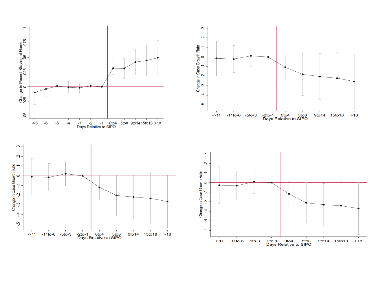
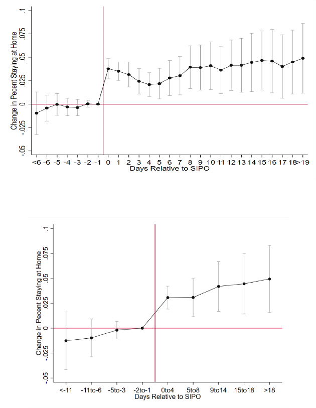
Panel (a) of Figure 2 visually presents the dynamics in stay-at-home behavior from an
event study analysis, highlighting three main points.
11
First, the lead pre-policy effects are close
to zero indicating that trends in social distancing between the SIPO-adopting and non-adopting
counties were parallel prior to enactment. Second, the marked increase in sheltering-at-home in
11
See Appendix Figure 2 for event study graphs based on alternate groupings of leads and lags, and the fully-
flexible non-grouped leads and lags by each day.
14
the treated counties relative to the non-adopters materializes only after the implementation of the
SIPO. Finally, the increase in social distancing within the treated counties remains sustained
through the observed post-treatment window. These localized results are in line with previous
state-level findings (Friedson et al. 2020; Dave et al. 2020), and confirm that shelter-at-home
orders proclaimed by local jurisdictions improved compliance with social distancing.
Given that social distancing inherently involves a decrease in person-to-person contact
for economic or non-economic reasons, we explore how these social distancing effects of
localized SIPOs vary depending on the county’s urbanicity and population density, both of which
are independent predictors of social interactions. Models reported in Panels II and III, based on
equation (2), consistently show that, while the orders were effective across the board in
encouraging individuals to shelter at home, the effects are significantly larger in urbanized and
more densely populated counties (3.4 percentage points vs. 1.6 to 1.7 percentage points in less
urban and sparsely populated counties).
Given this evidence that the local SIPOs were successful in inducing county residents to
stay at home, we then assess the public health effects of the local SIPO adoption, focusing on
county-level heterogeneity in the timing of the adoption, based on equation (3). These results are
presented in Table 2. The first column reports results from the most parsimonious specification
as a baseline for comparison. Here we find significant reductions in the COVID-19 case growth
following implementation of a local SIPO, but only for the earliest adopting counties. Growth in
cases fell by 13.5 percentage points within 4 days of implementation, and by 15.3 percentage
points within 8 days of implementation, a window of time that includes the 75
th
percentile of the
virus’s incubation period and, importantly, which also largely precedes the implementation of the
statewide SIPO. The effects accelerate as the post-policy window widens in length, with the

15
growth in COVID-19 cases declining on average by 19.4 percentage points following 18 days
after SIPO adoption. For later adopting counties, there are some suggestive declines in case
growth, though these are much smaller in magnitude and not statistically significant at
conventional levels.
In column (2), we add controls for county-specific linear and quadratic trends, based on
equation (4), to address the spatial heterogeneity within the state in the growth track of
confirmed cases (Appendix Figure 1). These controls serve an important purpose in accounting
for the exponential growth path of the outbreak prior to reaching its peak. For these models the
estimated SIPO effects are identified off deviations from each county’s growth path. As with the
results in column (1), the strongest reductions post-SIPO in the COVID-19 case growth rate
accrue to the earliest adopting counties, with benefits progressively increasing over time. After
18 days post-enactment, average daily growth in cases is 25.2 percent lower in these counties
relative to the later and non-adopting counties. With the addition of the trend controls, significant
decreases in case growth for the later-adopting counties also emerge, following their local
SIPOs, though the declines take a bit longer to materialize (after 5 to 8 days post-enactment) and
are somewhat smaller relative to the gains for the early-movers. We continue to find no
beneficial effects of the statewide-SIPO for the remaining counties that had not enacted local
orders.
The pattern and magnitudes remain largely unchanged after including additional COVID-
19 related policies and weather controls (columns 3 and 4, respectively).
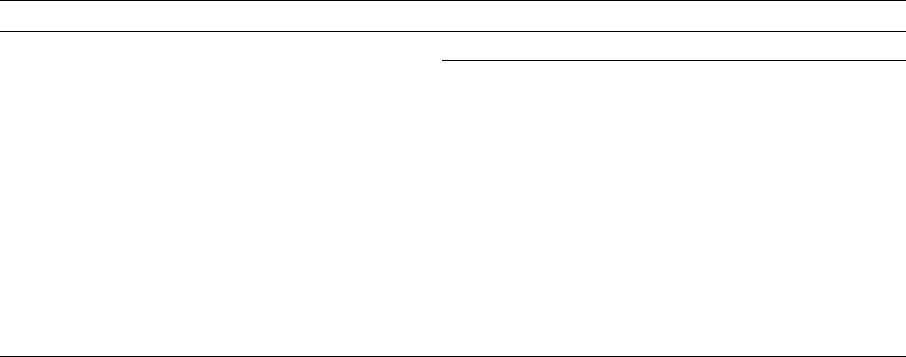
12
Panel (b) of Figure 2
presents the event study analysis for the early-adopting counties. Differential pre-treatment
12
We independently control for emergency declarations and non-essential business closure orders, which can
precede the adoption of a SIPO.

16
trends are flat, and there is a sharp and progressively larger decline in the average growth rates in
cases ensuing the adoption of the policy.
One potential concern with these estimates is that they may be confounded by differential
testing capabilities if access to testing is correlated with the timing of the localized SIPO
adoption.
13
Baseline differences in testing rates would be captured by the county fixed effects,
and the county linear trends go a long way towards addressing time-varying localized differences
in testing capacity, though not fully. To account for any residual systematic variation in testing
capacity, we draw on cumulative testing data obtained from the Texas Department of State
Health Services. In column (5), we restrict our analysis to only those counties that had achieved
a relatively high cumulative testing rate, at or above the state median.
14
This ensures a more
homogeneous set of localities with respect to testing availability. In spite of the large sample
restriction, the results remain remarkably robust, with no evidence that our estimates are driven
by local differences in testing.
Not all localities experienced the coronavirus outbreak at the same time. To ensure
comparability in the start of the outbreak cycle across counties, column (6) restricts the sample
such that a county enters the analysis only after it has experienced the start of the outbreak and
some level of community spread (at least two cases).
15
The final column accounts for any
potential border spillovers by controlling for the share of population in bordering counties that
13
In the presence of testing shortages, wherein tests are allocated to relatively sicker patients, confirmed counts of
COVID-19 cases are more likely to reflect severe cases, which is arguably a more salient indicator of infections for
studying the public health effects of a SIPO (Courtemanche et al. 2020a).
14
The earliest date that these data are available at the county level in a consistent format is April 8, which is when
we calculate the median testing rate. The median cumulative testing rate across TX counties was 10.7 (per 10,000
residents) as of April 8, and statewide mean was 24.9. Restricting the sample to counties with a cumulative testing
rate at the 60
th
(testing rate > 14.6) or at the 75
th
percentile (testing rate > 19.3), or counties with a testing rate that
exceeded the state mean (> 24.9) yields similar results and conclusions.
15
We also tested alternate thresholds, based on counties experiencing at least 1, 3, 4, and 5 confirmed cases, with
estimates remaining largely unchanged.

17
are covered by a SIPO.
16
Both sets of results continue to support the effectiveness of local
SIPOs among counties that adopted these orders well in advance of the statewide order.
The findings from Table 2 can be summarized as follows. Counties that implemented
their own local SIPOs, prior to the statewide order, experienced significant declines in the daily
case growth, with the strongest benefits accruing to the earliest adopters. Furthermore, the
decline in case growth accelerated over the post-policy window, with the growth rate reduced by
up to 26.2 percentage points for the early adopters and up to 21.1 percentage points for the later
adopting counties, from greater than 18 days following enactment.
In light of our earlier evidence that the effectiveness of local SIPOs is at least partly
propelled by an increase in social distancing, with stronger responses realized in urbanized and
highly populated localities, next we explore whether the public health effects also line up with
this spatial heterogeneity in the social distancing effects. Urbanicity and population density play
a key role in the propagation of infectious diseases across communities. Hence, these factors can
serve as multipliers that can enhance the efficacy of a given level of social distancing. In light of
this, the realized gains in public health from the SIPOs may be larger in urban and more
populated communities because of a larger social distancing effect induced by the SIPO (as
shown in Table 1) and also because of a larger marginal benefit of given level of social
distancing in more urban and populated localities.
Table 3 presents estimates of heterogeneous responses with respect to urbanicity and
population density, based on the fully-interacted formulation specified in equation (5). The
results show compelling evidence that virtually all of the decline in case growth accrued to
urbanized counties and highly populated counties that had adopted a localized shelter-in-place
16
Results are not sensitive to alternately controlling for whether any border county is covered by a local SIPO
(including SIPOs in neighboring states for those Texas counties that border other states).
18
order in advance of the statewide order. After 18 days following enactment, these counties
experienced significant declines in the daily growth rate of COVID-19 cases on the order of 26
to 27 percentage points. Evidence from the event study analyses for these sets of early adopting
urban and populous counties, shown in panels (c) and (d) of Figure 2, is consistent with common
pre-policy trends and a significant post-policy break in the trend. In contrast, less urban and
more sparsely populated counties did not reap any significant benefits from their local orders,
even if they enacted these orders well ahead of the statewide SIPO. The results in Table 3
continue to indicate that the statewide SIPO did not have any significant impact in flattening the
growth trajectory for the remaining non-adopting counties, regardless of their level of
urbanization or population density.
In a difference-in-differences estimator with the policy turning on at different times, as
with the differential timing of the SIPO adoption across the Texas counties, the treatment effect
is a weighted average of the many “mini” experiments comparing: (1) earlier-adopting counties
with later-adopters as controls; and (2) non-adopting counties (bound later by the statewide
order) with the earlier adopting counties as controls (Goodman-Bacon 2018). Hence, the effects
of the statewide SIPO for the non-adopting counties is necessarily identified by comparing their
conditional trends pre- and post-SIPO to those of the early adopters. This can be problematic. In
the presence of dynamic treatment effects, the early-adopters may not be a good counterfactual
for the non-adopters bound by the state order. As the trajectory of the early-adopting counties, at
the time when the statewide SIPO extends to the holdout counties, is still being affected by the
policy (that is, by the local SIPOs in the early moving counties), the estimated SIPO effects for
the non-adopting counties covered by the state order may be biased towards zero.

19
In order to assess this potential bias, and more cleanly identify the statewide SIPO effects
for the non-adopters, we draw on Goodman-Bacon (2018) and add county-level information
from other states that never adopted a statewide SIPO. By introducing another set of
counterfactuals – non-adopting counties in other states that were never bound by a statewide
order – we are able to derive plausibly consistent policy effects of the statewide SIPO in Texas
for the remaining non-adopting counties. Appendix Table 3 presents these results, using all non-
adopting states and alternately all bordering non-adopting states, as control groups. The
estimates and pattern of results remain robust. We continue to find that the declines in case
growth were driven primarily by the early-adopting urbanized and populated counties. There
was little to no benefit from issuing a statewide SIPO later, once these localized orders had
started to take effect.
4. Conclusions
By examining the staggered county implementations of SIPOs in Texas this study has
established two important results. First, when urbanized localities mobilize early with shelter-in-
place orders, the accrual of public health benefits are substantial. Second, in the presence of
early urban SIPO adopters, there may be little gains from a later blanket statewide order. These
findings are not surprising given the potential for exponential growth with the spread of disease.
Breaking the trend in cases, by acting earlier in areas where spread may be faster, has
compounding effects that can greatly alter the trajectory of an outbreak.
As a result, we find in Texas that almost all of the public health benefits from SIPO
implementation came from these urban, densely populated areas.
17
Our estimates indicate that
17
In supplemental analyses, available in Appendix Table 4, we explore other later-adopting SIPO states with more
limited early county SIPO adoption relative to the State of Texas. It is validating that results from these mini-
experiments in these states produced a pattern of results largely similar to Texas, suggesting that our findings are
generalizable.

20
91.5 percent of the reduction in the growth in COVID-19 cases came just from the early
localized adoption of SIPOs in urbanized counties alone.
18
There is very little gained from a
statewide order after this point.
These findings have large implications for the policy landscape going forward. In
particular, if the benefits of SIPOs are concentrated in urban areas, then the use of these
restrictive policies statewide may not be necessary when fighting outbreaks. More nuanced
policy strategies that are stricter in dense urban areas and looser in less dense rural areas may
yield similar health benefits without imposing the costs, both in terms of economic activity and
in terms of inconvenience on part of the population.
18
Much of the leftover gains accrues from the later adopting urbanized counties, who are doing so still in advance of
the statewide SIPO. See Appendix Table 5 for a discussion of this calculation.

21
References
Allday, Erin. 2020. “Bay Area Orders ‘Shelter in Place,’ Only Essential Businesses Open in 6
Counties.” San Francisco Chronicle, March 16. Available at:
https://www.sfchronicle.com/local-politics/article/Bay-Area-must-shelter-in-place-Only-
15135014.php
Baek, ChaeWon, Peter B. McCrory, Todd Messer, and Preston Mui. 2020. “Unemployment
Effects of Stay-at-Home Orders: Evidence from High Frequency Claims Data.” Institute
for Research on Labor and Employment Working Paper No. 101-20.
Bai, Yan, Lingsheng Yao, Tao Wei, Fei Tian, Dong-Yan Jin, Lijuan Chen, and Meiyun Wang.
2020. "Presumed asymptomatic carrier transmission of COVID-19." JAMA, 323(14):
1406-1407.
Bertrand, Marianne, Esther Duflo, and Sendhil Mullainathan. 2004. “How much should we trust
differences-in-differences estimates?” The Quarterly Journal of Economics, 119(1): 249-
275.
Centers for Disease Control. 2020. “COVID-19 How to Protect Yourself and Others.” Available
online: https://www.cdc.gov/coronavirus/2019-ncov/prevent-getting-sick/prevention.html
Courtemanche, Charles, Joseph Garuccio, Anh Le, Joshua C. Pinkston, and Aaron Yelowitz.
2020a. “Strong Social Distancing Measures In The United States Reduced The COVID-
19 Growth Rate.” Health Affairs, in press.
Courtemanche, Charles J., Joseph Garuccio, Anh Le, Joshua C. Pinkston, and Aaron Yelowitz.
2020b. "Did Social-Distancing Measures in Kentucky Help to Flatten the COVID-19
Curve?" Institute for the Study of Free Enterprise Working Paper 2020-4.
Dave, Dhaval M., Andrew I. Friedson, Kyutaro Matsuzawa, and Joseph J. Sabia. 2020. “When
Do Shelter-In-Place Orders Fight COVID-19 Best? Policy Heterogeneity across States
and Adoption Time.” National Bureau of Economic Research Working Paper No. 27091.
Defense Casualty Analysis System. 2008. “Vietnam War U.S. Military Fatal Casualty Statistics.”
Available online: https://www.archives.gov/research/military/vietnam-war/casualty-
statistics
Friedson, Andrew I., Drew McNichols, Joseph J. Sabia, and Dhaval Dave. 2020. “Did
California’s Shelter-in-Place Order Work? Early Coronavirus-Related Public Health
Effects.” National Bureau of Economic Research Working Paper No. 26992.
Goodman-Bacon, Andrew. 2018. “Difference-in-Differences with Variation in Treatment
Timing.” National Bureau of Economic Research Working Paper No. 25108.
Holshue, Michelle L., Chas DeBolt, Scott Lindquist, Kathy H. Lofy, John Wiesman, Hollianne
Bruce, Christopher Spitters, et al. 2020. “First case of 2019 novel coronavirus in the
United States.” New England Journal of Medicine, 382: 929-936.
Johns Hopkins University. 2020. “COVID-19 Case Tracker.” Available online:
https://coronavirus.jhu.edu/map.html
Lauer, Stephen A., Kyra H. Grantz, Qifang Bi, Forrest K. Jones, Qulu Zheng, Hannah R.
Meredith, Andrew S. Azman, Nicholas G. Reich, and Justin Lessler. 2020. “The
Incubation Period of Coronavirus Disease 2019 (COVID-19) from Publicly Reported
Confirmed Cases: Estimation and Application.” Annals of Internal Medicine

22
Mervosh, Sarah, Denise Lu, and Vanessa Swales. “See Which States and Cities Have Told
Residents to Stay at Home.” The New York Times, April 7. Available at:
https://www.nytimes.com/interactive/2020/us/coronavirus-stay-at-home-order.html
National Association of Counties. 2020. “County Declarations and Policies In Response to
COVID-19 Pandemic.” Available at: https://ce.naco.org/?dset=COVID-
19&ind=Emergency%20Declaration%20Types
Pan, Xingfei, Dexiong Chen, Yong Xia, Xinwei Wu, Tangsheng Li, Xueting Ou, Liyang Zhou,
and Jing Liu. 2020. “Asymptomatic cases in a family cluster with SARS-CoV-2
infection.” The Lancet Infectious Diseases, 20(4): 410-411.
Rothe C, Schunk M, Sothmann P, et al. 2020. “Transmission of 2019-nCoV Infection from an
Asymptomatic Contact in Germany.” New England Journal of Medicine, 382:970-971.
Wilson, Steven G., David A. Plane, Paul J. Mackun, Thomas R. Fischetti, and Justyna
Goworowska. 2020. “Patterns of Metropolitan and Micropolitan Population Change 2000
to 2020.” 2010 Census Special Reports. U.S. Census Bureau. Report C2020SR-01.
23
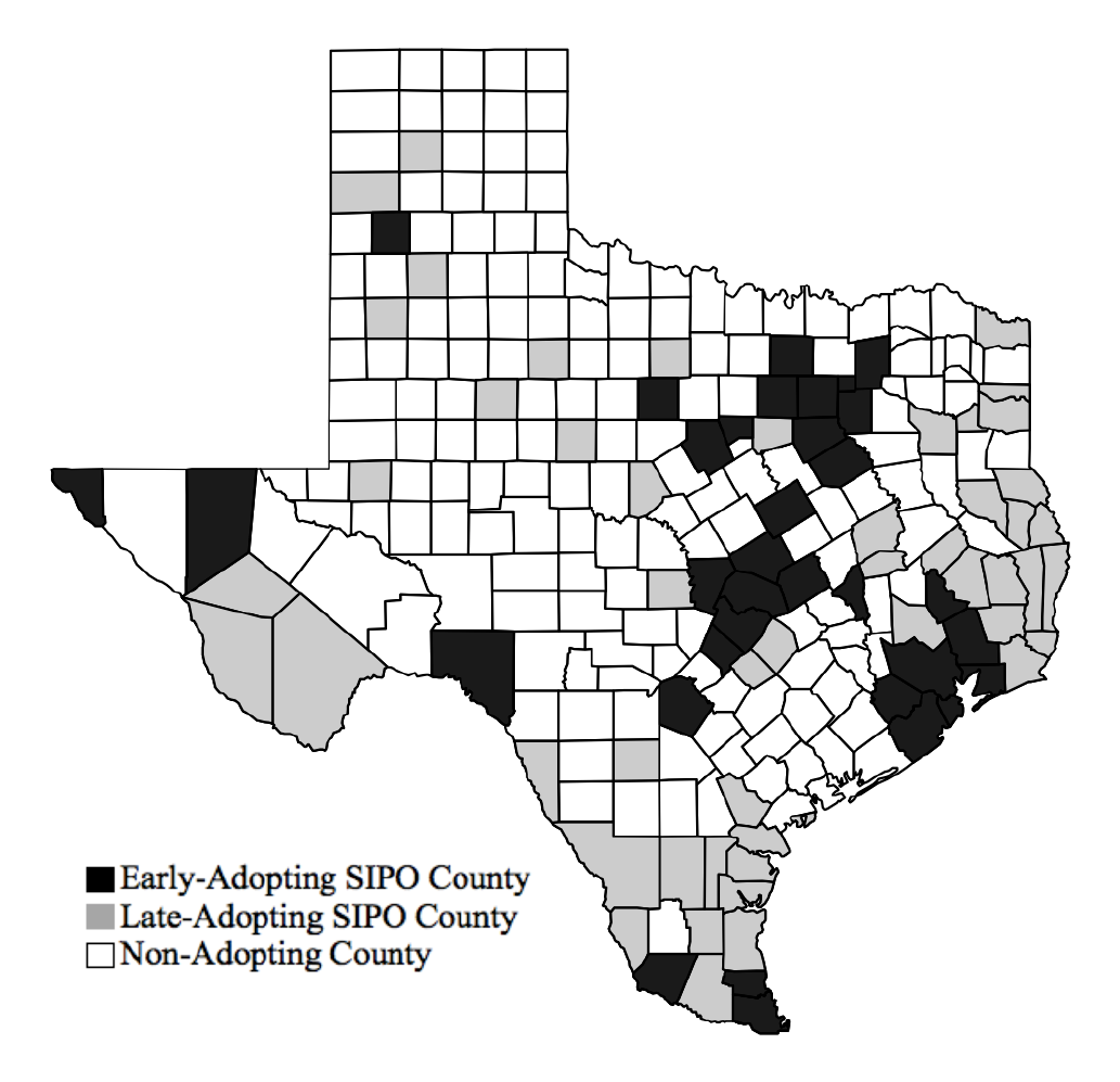
Figure 1: Enactment of County Shelter-in-Place Orders in Texas
Notes: Counties that adopted SIPO on March 26 or before are defined as Early-Adopting SIPO Counties; counties
that adopted SIPO between March 27 and April 1 are defined as Late-Adopting SIPO Counties; and counties that
never adopted a SIPO (but were bound by the statewide order) are defined as Non-Adopting Counties.
24
Panel (a): Percent Staying at Home Full-Time
Notes: Estimates are obtained using weighted least squares regression. The model includes the following controls: an indicator for whether thecounty had
issued a non-essential business closure order, an indicator for whether the county had issued an emergency declaration, the average temperature (in degrees
Celsius) in the county, an indicator for whether measurable precipitation fell in the county, county fixed effects, day fixed effects, and a county-specific
quadratic time trend. Standard errors are clustered at the county-level.
Figure 2: Event-Study Analyses of Effects of Shelter-In-Place Orders on Social Distancing and COVID-19 Case Growth
Panel (b): COVID-19 Growth for Early-Adopting SIPO Counties
Panel (c): COVID-19 Growth for Urban Early SIPO Counties
Panel (d): COVID-19 Growth for High Population Density Early
SIPO Counties

25
Table 1: Difference-in-Differences Estimates of Effect of Shelter-in-Place Orders on
Percent Staying at Home Full-Time
(1)
(2)
(3)
(4)
Panel I: Difference-in-Difference Estimate
SIPO
0.024***
0.030***
0.030***
0.029***
(0.005)
(0.006)
(0.006)
(0.006)
Panel II: Heterogeneous Treatment Effect by Urbanicity
SIPO * ≥ 75% Urbanicity
0.033***
0.034***
0.034***
0.034***
(0.006)
(0.007)
(0.008)
(0.008)
SIPO * < 75% Urbanicity
0.007
0.016***
0.016***
0.016***
(0.005)
(0.005)
(0.005)
(0.005)
Panel III: Heterogeneous Treatment Effect by Population Density
SIPO * ≥ 150 People Per Sq. Mi
0.033***
0.034***
0.034***
0.034***
(0.007)
(0.007)
(0.008)
(0.008)
SIPO * < 150 People Per Sq. Mi
0.008
0.017***
0.017***
0.017***
(0.006)
(0.005)
(0.005)
(0.005)
N
12954
12954
12954
12954
County & Day Fixed Effects?
Yes
Yes
Yes
Yes
County Time Trend?
No
Yes
Yes
Yes
NEBCO and Emergency?
No
No
Yes
Yes
Weather Controls?
No
No
No
Yes
Notes: Estimates are obtained using weighted least squares regression. The model includes the following controls: an indicator for
whether the county had issued a non-essential business closure order, an indicator for whether the county had issued an emergency
declaration, the average temperature (in degrees Celsius) in the county, an indicator for whether measurable precipitation fell in the
county, county fixed effects, day fixed effects, and a county-specific quadratic time trend. Standard errors, clustered at the county-level,
are reported in parenthesis.

26
Table 2: Difference-in-Differences Estimates of Effect of Shelter-in-Place Orders on COVID-19 Case Growth
(1)
(2)
(3)
(4)
(5)
(6)
(7)
Early-Adopting SIPO Counties
0-4 Days After
-0.135***
-0.158***
-0.152***
-0.150***
-0.171***
-0.128**
-0.118**
(0.043)
(0.042)
(0.044)
(0.043)
(0.048)
(0.052)
(0.055)
5-8 Days After
-0.153***
-0.196***
-0.186***
-0.184***
-0.202***
-0.166**
-0.154**
(0.055)
(0.055)
(0.058)
(0.058)
(0.066)
(0.081)
(0.072)
9-18 Days After
-0.164**
-0.218***
-0.207***
-0.210***
-0.220***
-0.176**
-0.181**
(0.068)
(0.068)
(0.072)
(0.072)
(0.080)
(0.084)
(0.083)
>18 Days After
-0.194***
-0.252***
-0.242***
-0.251***
-0.262***
-0.207**
-0.222***
(0.071)
(0.067)
(0.070)
(0.070)
(0.078)
(0.086)
(0.082)
Late-Adopting SIPO Counties
0-4 Days After
0.014
-0.035
-0.031
-0.031
-0.049
-0.069
-0.001
(0.050)
(0.051)
(0.049)
(0.049)
(0.057)
(0.059)
(0.059)
5-8 Days After
-0.038
-0.107*
-0.102*
-0.105*
-0.120*
-0.125**
-0.072
(0.056)
(0.057)
(0.057)
(0.058)
(0.066)
(0.060)
(0.069)
9-18 Days After
-0.054
-0.142**
-0.136**
-0.141**
-0.155**
-0.150**
-0.108*
(0.055)
(0.055)
(0.055)
(0.054)
(0.062)
(0.061)
(0.065)
>18 Days After
-0.078
-0.197***
-0.191***
-0.197***
-0.211***
-0.181***
-0.162**
(0.059)
(0.061)
(0.061)
(0.061)
(0.067)
(0.064)
(0.068)
Non-Adopting Counties Bound by State SIPO
0-4 Days After
-0.054
-0.031
-0.026
-0.030
-0.039
-0.074*
-0.001
(0.033)
(0.040)
(0.044)
(0.044)
(0.049)
(0.043)
(0.053)
5-8 Days After
-0.033
0.019
0.025
0.020
0.004
-0.059
0.048
(0.036)
(0.049)
(0.053)
(0.053)
(0.060)
(0.047)
(0.059)
9-18 Days After
-0.053
0.055
0.063
0.051
0.049
-0.053
0.077
(0.040)
(0.069)
(0.074)
(0.072)
(0.084)
(0.061)
(0.076)
>18 Days After
-0.049
0.154
0.164
0.142
0.152
-0.004
0.168
(0.041)
(0.105)
(0.109)
(0.105)
(0.127)
(0.086)
(0.105)
N
12954
12954
12954
12954
6477
4878
12954
County & Day Fixed Effects?
Yes
Yes
Yes
Yes
Yes
Yes
Yes
County Time Trend?
No
Yes
Yes
Yes
Yes
Yes
Yes
NEBCO & Emergency Declaration?
No
No
Yes
Yes
Yes
Yes
Yes
Weather Controls?
No
No
No
Yes
Yes
Yes
Yes
Testing Rate ≥ Median?
No
No
No
No
Yes
No
No
Sample w/ Cases ≥ 2
No
No
No
No
No
Yes
No
Weighted Population Share of
Border Counties w/ SIPO
No
No
No
No
No
No
Yes
27
Notes: Estimates are obtained using weighted least squares regression. The model includes the following controls:
an indicator for whether the county had issued a non-essential business closure order, an indicator for whether the
county had issued an emergency declaration, the average temperature (in degrees Celsius) in the county, an indicator
for whether measurable precipitation fell in the county, county fixed effects, day fixed effects, and a county-specific
quadratic time trend. Standard errors, clustered at the county-level, are reported in parenthesis. Counties that adopted
SIPO on March 26 or before are defined as Early-Adopting SIPO Counties, and counties that adopted SIPO between
March 27 and April 1 are defined as Late-Adopting SIPO Counties.

28
Table 3. Heterogeneity in Effects of Shelter-in-Place Orders on COVID-19 Case Growth, by
Urbanicity and Population Density
Urbanicity
Population Density
≥ 75%
< 75%
≥ 150 persons per
sq-mi
< 150 persons per
sq-mi
(1)
(2)
(3)
(4)
Early-Adopting SIPO Counties
0-4 Days After
-0.161***
-0.052
-0.162***
-0.014
(0.043)
(0.044)
(0.043)
(0.053)
5-8 Days After
-0.200***
-0.013
-0.201***
-0.004
(0.057)
(0.051)
(0.058)
(0.047)
9-18 Days After
-0.219***
-0.060
-0.223***
-0.035
(0.070)
(0.060)
(0.072)
(0.061)
>18 Days After
-0.259***
-0.078
-0.264***
-0.061
(0.067)
(0.070)
(0.068)
(0.070)
Late-Adopting SIPO Counties
0-4 Days After
-0.040
-0.009
-0.047
-0.003
(0.057)
(0.048)
(0.060)
(0.049)
5-8 Days After
-0.132**
-0.029
-0.144**
-0.031
(0.062)
(0.055)
(0.062)
(0.056)
9-18 Days After
-0.184***
-0.016
-0.190***
-0.032
(0.055)
(0.055)
(0.056)
(0.068)
>18 Days After
-0.263***
-0.010
-0.268***
-0.034
(0.064)
(0.062)
(0.065)
(0.093)
Non-Adopting Counties Bound by State SIPO
0-4 Days After
-0.040
-0.019
-0.061
-0.013
(0.054)
(0.039)
(0.059)
(0.042)
5-8 Days After
-0.001
0.041
-0.015
0.043
(0.077)
(0.047)
(0.082)
(0.052)
9-18 Days After
0.075
0.040
0.073
0.044
(0.117)
(0.063)
(0.123)
(0.068)
>18 Days After
0.203
0.107
0.222
0.108
(0.194)
(0.090)
(0.203)
(0.097)
N
12954
12954
12954
12954
Notes: Estimates are obtained using weighted least squares regression. The model includes the following controls: an indicator
for whether the county had issued a non-essential business closure order, an indicator for whether the county had issued an
emergency declaration, the average temperature (in degrees Celsius) in the county, an indicator for whether measurable
precipitation fell in the county, county fixed effects, day fixed effects, and a county-specific quadratic time trend. Standard errors,
clustered at the county-level, are reported in parenthesis. Counties that adopted SIPO on March 26 or before are defined as Early-
Adopting SIPO Counties, and counties that adopted SIPO between March 27 and April 1 are defined as Late-Adopting SIPO
Counties.
29
Online Appendix Figures and Tables
30
Appendix Figure 1: Trends in Texas COVID-19 Cases
31
Appendix Figure 2: Event Studies Analysis of Effect of SIPOs on Percent Staying at Home
(a) Individual Leads and Lags
(c) Grouped Leads and Lags

32
Appendix Table 1: Means of Dependent and independent Variables
Dependent Variables
Percent Staying at Home
0.359
(0.077)
Log Case Growth
0.112
(0.192)
Independent Variables
SIPO
0.648
(0.478)
NEBCO
a
0.039
(0.194)
Emergency Declarations
0.890
(0.313)
Average Temperature (°C)
19.077
(4.768)
Any Precipitation
0.414
(0.493)
Notes: Means are weighted using the county population.
a
NEBCO denotes a county with a full NEBCO, but without a full SIPO.
33
Appendix Table 2: Coefficients on Control Variables for Column (4) of Tables 1 and 2
(1)
(2)
% Staying at Home
Case Growth
NEBCO
-0.000
0.005
(0.003)
(0.023)
Emergency Order
-0.002
0.019
(0.004)
(0.020)
Average Temperature
-0.000**
0.003
(0.000)
(0.003)
Any Precipitation
0.006***
0.025**
(0.001)
(0.011)
N
12954
12954
Notes: Estimates are obtained using weighted least squares regression. The model includes the following
controls: an indicator for whether the county had issued a non-essential business closure order, an indicator
for whether the county had issued an emergency declaration, the average temperature (in degrees Celsius) in
the county, an indicator for whether measurable precipitation fell in the county, county fixed effects, day fixed
effects, and a county-specific quadratic time trend. Standard errors, clustered at the county-level, are reported
in parenthesis.

34
Appendix Table 3: Estimated Effect of SIPOs on COVID-19 Cases in Texas,
Including Non-Adopting SIPO States as Controls
(1)
(2)
(3)
Early-Adopting SIPO Counties
0-4 Days After
-0.150***
-0.116***
-0.075*
(0.043)
(0.042)
(0.039)
5-8 Days After
-0.184***
-0.129***
-0.102***
(0.058)
(0.045)
(0.035)
9-18 Days After
-0.210***
-0.113**
-0.098**
(0.072)
(0.052)
(0.041)
>18 Days After
-0.251***
-0.147***
-0.126***
(0.070)
(0.048)
(0.035)
Late-Adopting SIPO Counties
0-4 Days After
-0.031
0.013
-0.004
(0.049)
(0.036)
(0.030)
5-8 Days After
-0.105*
-0.029
-0.042*
(0.058)
(0.037)
(0.025)
9-18 Days After
-0.141**
-0.063*
-0.054**
(0.054)
(0.034)
(0.025)
>18 Days After
-0.197***
-0.128***
-0.076
(0.061)
(0.046)
(0.047)
Non-Adopting Counties Bound by State SIPO
0-4 Days After
-0.030
0.016
0.002
(0.044)
(0.026)
(0.020)
5-8 Days After
0.020
0.063*
0.031
(0.053)
(0.036)
(0.030)
9-18 Days After
0.051
0.066
0.021
(0.072)
(0.057)
(0.053)
>18 Days After
0.142
0.117
0.042
(0.105)
(0.097)
(0.095)
N
12954
20706
45237
Inclusion of Border Non-Adopting SIPO States?
No
Yes
Yes
Inclusion of All Non-Adopting SIPO States?
No
No
Yes
Notes: Estimates are obtained using weighted least squares regression. The model includes the following controls: an indicator
for whether the county had issued a non-essential business closure order, an indicator for whether the county had issued an
emergency declaration, the average temperature (in degrees Celsius) in the county, an indicator for whether measurable
precipitation fell in the county, county fixed effects, day fixed effects, and a county-specific quadratic time trend. Standard errors,
clustered at the county-level, are reported in parenthesis. Counties that adopted SIPO on March 26 or before are defined as Early-
Adopting SIPO Counties, and counties that adopted SIPO between March 27 and April 1 are defined as Late-Adopting SIPO
Counties. Border Non-Adopting SIPO states include AR and OK. Other Non-Adopting SIPO states include IA, KY, ND, NC,
NE, SD, UT and WY. We excluded Morgan county and Weber county in Utah that adopted a county SIPO on 4/2 from our
analysis.

35
Appendix Table 4: Estimated Effect of SIPOs on COVID-19 Cases for Other Late Adopting SIPO
States (Including All Non-Adopting SIPO States as Controls)
PA
MO
FL
GA
(1)
(2)
(3)
(4)
Early-Adopting SIPO Counties
0-4 Days After
-0.006
0.063
-0.114***
-0.027
(0.029)
(0.056)
(0.035)
(0.028)
5-8 Days After
-0.081**
-0.042
-0.136***
-0.085***
(0.035)
(0.043)
(0.053)
(0.026)
9-18 Days After
-0.098***
-0.091**
-0.191***
-0.088***
(0.032)
(0.041)
(0.035)
(0.027)
>18 Days After
-0.113***
-0.140***
-0.157***
-0.076
(0.032)
(0.051)
(0.036)
(0.048)
Late-Adopting SIPO Counties
0-4 Days After
-0.010
-0.052
-0.095***
-0.083***
(0.024)
(0.033)
(0.014)
(0.023)
5-8 Days After
-0.011
-0.074***
-0.128***
-0.087***
(0.018)
(0.016)
(0.017)
(0.020)
9-18 Days After
-0.051*
-0.054**
-0.107***
-0.065***
(0.026)
(0.027)
(0.021)
(0.024)
>18 Days After
-0.051
-0.007
-0.071**
-0.032
(0.049)
(0.044)
(0.035)
(0.037)
Non-Adopting Counties Bound by State SIPO
0-4 Days After
0.075**
0.040**
-0.033***
0.009
(0.031)
(0.015)
(0.013)
(0.013)
5-8 Days After
0.084***
0.011
-0.045***
-0.023
(0.031)
(0.020)
(0.016)
(0.017)
9-18 Days After
0.061
0.008
-0.042
-0.035
(0.038)
(0.031)
(0.026)
(0.027)
>18 Days After
0.035
-0.015
-0.035
-0.076*
(0.056)
(0.042)
(0.043)
(0.043)
N
35547
38250
35802
40494
Notes: Estimates are obtained using weighted least squares regression. The model includes the following controls: an indicator for whether the
county had issued a non-essential business closure order, an indicator for whether the county had issued an emergency declaration, the average
temperature (in degrees Celsius) in the county, an indicator for whether measurable precipitation fell in the county, county fixed effects, day fixed
effects, and a county-specific quadratic time trend. Standard errors, clustered at the county-level, are reported in parenthesis. PA counties that
adopted SIPO on March 23 or before, MO counties that adopted SIPO on March 25 or before, and GA and FL counties that adopted SIPO on March
26 or before are defined as Early-Adopting SIPO Counties; and PA counties that adopted SIPO between March 24 and April 1, MO counties that
adopted SIPO between March 26 and April 6, and GA and FL counties that adopted SIPO between March 27 and April 3 are defined as Late-
Adopting SIPO Counties. For column (1), PA analysis, we excluded Davis county, Morgan county, Utah county, Wasatch county and Weber county
in Utah that adopted a county SIPO on 4/1 or 4/2 from our analysis.

36
Appendix Table 5: Calculation of Decomposition of SIPO-Induced Decline in Texas
COVID-19 Case Growth
We utilize equation (5) (with estimates reported in Table 3) to perform the decomposition as
follows. First, we compute the actual observed weighted (based on county population)
average daily case growth in Texas across all counties and days over our sample period. This
observed growth rate (denoted G1) reflects the presence of all SIPOs, localized and statewide,
and when they were enacted. Next, we compute the weighted average daily case growth
(denoted G2) under the counterfactual scenario wherein no SIPOs at all (either localized or
statewide) have been enacted. We do this, based on Equation (5), by netting out the estimated
effects of all SIPOs using the estimated coefficients for the three groups of counties from the
observed growth rate. The difference (G2 – G1) then represents the average reduction in the
daily case growth in the state due to all shelter-in-place orders.
In order to compute how much of this total policy response is driven by the early adopting
urbanized counties, we compute the weighted average daily case growth (denoted G3) under
another counterfactual scenario such that only the early urbanized jurisdictions adopted their
SIPOs, and assume no other SIPOs (later adopters, non-urban counties, or statewide SIPO)
have been adopted. To compute this counterfactual growth rate, we subtract out from the
observed growth rate the estimated effect of all other SIPOs, except for the early urban
localities’ orders, utilizing the coefficients estimated reported in Table 3. The difference (G3 –
G2) represents the reduction in the average daily growth in the state if only the early urban
jurisdictions had enacted their orders, and there were no other subsequent orders. Finally, the
ratio, [(G3-G2)]/[(G2-G1)], can be interpreted as the percent of the observed growth reduction
from the SIPOs that is driven by only the early adopting urbanized county orders.
