ROCCurve.ps

Data Mining Methods for Recommender

Systems

Xavier Amatriain, Alejandro Jaimes, Nuria Oliver, and Josep M. Pujol

Abstract In this chapter, we give an overview of the main Data Mining techniques

that are applied in the context of Recommender Systems. We ﬁrst describe common

preprocessing methods such as sampling or dimensionality reduction. Next, we re-

view a the most important classiﬁcation techniques, including Bayesian Networks

and Support Vector Machines. We describe the so popular k-means clustering algo-

rithm and discuss several alternatives. We also present association rules and present

algorithms for an efﬁcient training process. In addition to introducing these tech-

niques, we survey their uses in Recommender Systems and present cases where

they have been successfully applied.

1 Introduction

Recommender Systems (RS) typically apply techniques and methodologies from

other neighboring areas – such as Human Computer Interaction (HCI) or Infor-

mation Retrieval (IR). However, most of these systems bear in their core an algo-

rithm that can be understood as a Data Mining (DM) technique. In fact, most of

the challenges in Data Mining [65] are also challenges in Recommender Systems

Xavier Amatriain

Telefonica Research, Via Augusta, 122, Barcelona 08021, e-mail:

xar@tid.es

Alejandro Jaimes

Telefonica Research, Emilio Vargas, 6, Madrid 28043 e-mail:

ajaimes@tid.es

Nuria Oliver

Telefonica Research, Via Augusta, 122, Barcelona 08021 e-mail:

nuriao@tid.es

Josep M. Pujol

Telefonica Research, Via Augusta, 122, Barcelona 08021 e-mail:

jmps@tid.es

with the important exception of those related to user interface design

2 Xavier Amatriain, Alejandro Jaimes, Nuria Oliver, and Josep M. Pujol

Scalability, Dimensionality, Complex and Heterogeneous Data, Data Quality, Data

Ownership and Distribution, Privacy Preservation, and Streaming Data.

There are many deﬁnitions for Data Mining. In the context of this chapter, we

will deﬁne Data Mining as the “non-trivial extraction of meaningful information

from large amounts of data by automatic or semi-automatic means”. Data Mining

uses methods and techniques drawn from machine learning, artiﬁcial intelligence,

statistics, and database systems. However most of these “traditional” techniques

need to be adapted to account for the high dimensionality and heterogeneity of data

that is pervasive in Data Mining problems.

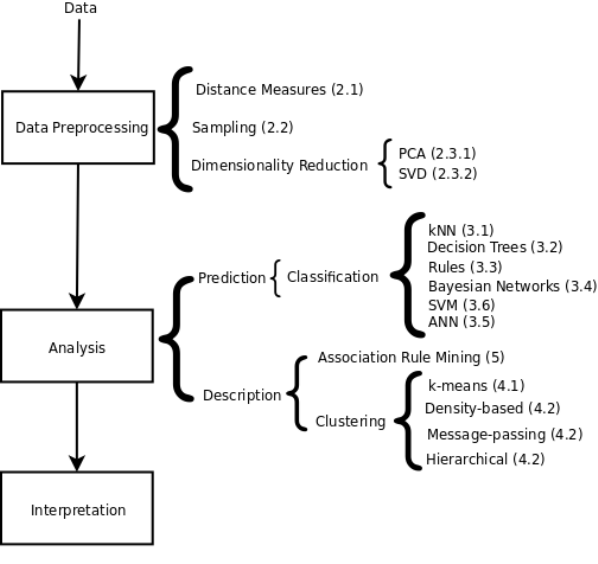
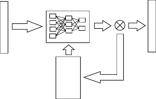
The process of data mining typically consists of 3 steps, carried out in succession:

Data Preprocessing [53], Data Analysis, and Result Interpretation (see Figure

1).

Fig. 1: Main steps and methods in a Data Mining problem, with their correspon-

dence to chapter sections.

We will analyze some of the most important methods for data preprocessing in

Section

2. In particular, we will focus on sampling, dimensionality reduction, and

the use of distance functions because of their signiﬁcance and their role in recom-

mender systems.

Data Mining Methods for Recommender Systems 3

We usually distinguish two kinds of methods in the analysis step: predictive and

descriptive. Predictive methods use a set of observed variables to predict future or

unknown values of other variables. Prediction methods include classiﬁcation, re-

gression and deviation detection. Descriptive methods focus on ﬁnding meaningful

patterns that help understand and interpret the data. These include clustering, asso-

ciation rule discovery and pattern discovery. Both kinds of methods can be used in

the context of a recommender system.

In Sections 3 through 5, we provide an overview introduction to the analysis

methods that are most commonly used in Recommender Systems: classiﬁcation,

clustering and association rule discovery (see Figure

1 for a detailed view of the

different topics covered in the chapter).

Note that this chapter does not intend to give a thorough review of Data Mining

methods, but rather to highlight the impact that Data Mining algorithms have in the

Recommender Systems ﬁeld, and to provide an overview of the key Data Mining

techniques that have been successfully used. We shall direct the interested reader to

Data Mining textbooks (see [25, 65], for example) or the more focused references

that are provided throughout the chapter. Most of the algorithms and techniques

presented in this chapter are also implemented in general purpose machine learning

frameworks such as Weka [66] or Torch [17], or even mathematics and statistical

packages such as Matlab

 [64] or Octave [22].

2 Data Preprocessing

We deﬁne data as a collection of objects and their attributes, where an attribute is

deﬁned as a property or characteristic of an object. Other names for object include

record, item, point, sample, observation, or instance. An attribute might be also be

referred to as a variable, ﬁeld, characteristic, or feature.

There are different types of data with attributes of varied nature. In addition, real-

life data typically needs to be preprocessed (e.g. cleansed, ﬁltered, transformed) in

order to be used by the machine learning techniques in the analysis step. There

might be missing points, duplicated data, or noise, for instance.

In this section, we focus on three issues that are of particular importance when

designing a recommender system. First, we review different similarity or distance

measures between data points or collections of data points. Next, we discuss the

issue of sampling as a way to reduce the number of items in very large collections

while preserving its main characteristics, or as a way to separate a training and

testing data set. Finally, we describe the most common techniques to reduce the

dimensionality of the data.

4 Xavier Amatriain, Alejandro Jaimes, Nuria Oliver, and Josep M. Pujol

2.1 Similarity Measures

We deﬁne similarity as a numerical measure – often falling in the [0,1] range – of

how alike two items are. Having an appropriate similarity function is a key issue

for many data mining algorithms. We usually refer to the distance function, d, as a

numerical measure of how different two items are.

The most common distance measure is the Euclidean distance:

d(x,y) =

∑

k=1

− y

)

(1)

where n is the number of dimensions (attributes) and x

and y

are the k

attributes

(components) of data objects x and y, respectively. Note that in order to compute the

Euclidean distance, it is necessary to normalize the data if scales differ.

The Minkowski Distance is a generalization of Euclidean Distance:

d(x,y) = (

∑

k=1

− y

)

(2)

where r is the degree of the distance. Depending on the value of r, the generic

Minkowski distance is known with speciﬁc names: For r = 1, the city block, (Man-

hattan, taxicab or L1 norm) distance; For r = 2, the Euclidean distance; For r → ∞,

the supremum (L

max

norm or L

∞

norm) distance, which corresponds to computing

the maximum difference between any dimension of the data objects.

The Mahalanobis distance is deﬁned as:

d(x,y) =

(x− y)

−1

(x− y)

(3)

where

is the covariance matrix of the data.

Another very common approach is to consider items as document vectors of an

n-dimensional space and compute their similarity as the cosine of the angle that they

form:

cos(x,y) =

(x• y)

||x||||y||

(4)

where • indicates vector dot product and ||x|| is the norm of vector x. This similarity

is known as the cosine similarity or the L2 Norm.

The similarity between items can also be given by their correlation which mea-

sures the linear relationship between objects. While there are several correlation

coefﬁcients that may be applied, the Pearson correlation is the most commonly

used:

Pearson(x,y) =

(x,y)

(5)

, where

is the covariance of data points x and y and

is their standard deviation.

Finally, several similarity measures have been proposed in the case of items that

only have binary attributes. First, the following quantities are computed: M01 = the

Data Mining Methods for Recommender Systems 5

number of attributes where x was 0 and y was 1, M10 = the number of attributes

where x was 1 and y was 0, M00 = the number of attributes where x was 0 and y was

0, M11 = the number of attributes where x was 1 and y was 1.

From those quantities we can compute:

1. The Simple Matching coefﬁcient (SMC):

SMC =

numberofmatches

numberofattributes

M11+ M00

M01+ M10+ M00+ M11

(6)

2. The Jaccard coefﬁcient (JC):

JC =

M11

M01+ M10+ M11

(7)

3. The Extended Jaccard (Tanimoto) coefﬁcient (EJC): It is a variation of JC for

continuous or count attributes.

d =

x• y

kxk

+ kxk

− x• y

(8)

2.1.1 Similarity Measures in Recommender Systems

The most common approach to collaborative ﬁltering in Recommender Systems is

to use the kNN classiﬁer that will be described in Section

3.1. This classiﬁcation

method – as most classiﬁers and clustering techniques – is highly dependent on

deﬁning an appropriate similarity measure.

Recommender Systems have traditionally used either the cosine similarity (see

Eq.

4) or the Pearson correlation (see Eq. 5) – or one of their many variations

through, for instance, weighting schemes – as the similarity measure. However,

most of the other distance measures previously reviewed are possible in this con-

text. Spertus et al. [62] did a large-scale study to evaluate six different similarity

measures in the context of the Orkut social network. Although their results might be

biased by the particular setting of their experiment, it is interesting to note that the

best response to recommendations were to those generated using the cosine similar-

ity. Lathia et al. [44] also carried out a study of several similarity measures where

they concluded that, in the general case, the prediction accuracy of a recommender

system was not affected by the choice of the similarity measure. As a matter of

fact and in the context of their work, using a random similarity measure sometimes

yielded better results than using any of the well-known approaches.

2.2 Sampling

Sampling is the main technique used in data mining for selecting a subset of rele-

vant data from a large data set. It is used both in the preprocessing and ﬁnal data

6 Xavier Amatriain, Alejandro Jaimes, Nuria Oliver, and Josep M. Pujol

interpretation steps. Sampling may be used because processing the entire data set

is computationally too expensive. It can also be used to create training and testing

datasets. In this case, the training dataset is used to learn the parameters or conﬁgure

the algorithms used in the analysis step, while the testing dataset is used to evalu-

ate the model or conﬁguration obtained in the training phase, making sure that it

performs well (i.e. generalizes) with previously unseen data.

The key issue to sampling is ﬁnding a subset of the original data set that is repre-

sentative – i.e. it has approximately the same property of interest – of the entire set.

The simplest sampling technique is random sampling, where there is an equal prob-

ability of selecting any item. However more sophisticated approaches are possible.

For instance, in stratiﬁed sampling the data is split into several partitions based on

a particular feature, followed by random sampling on each partition independently.

The most common approach to sampling consists of using sampling without re-

placement: When an item is selected, it is removed from the population. However, it

is also possible to perform sampling with replacement, where items are not removed

from the population once they have been selected, allowing for the same sample to

be selected more than once.

It is common practice to use standard random sampling without replacement with

an 80/20 proportion when separating the training and testing data sets. This means

that we use random sampling without replacement to select 20% of the instances

for the testing set and leave the remaining 80% for training. Note that the 80/20

proportion should be taken as a rule of thumb: It is generally the case that any value

over 2/3 for the training set is appropriate.

Sampling can lead to an over-specialization to the particular division of the train-

ing and testing data sets. For this reason, the training process is repeated K times as

follows: the training and test sets are created from the original data set, the model

is trained using the training data and tested with the examples in the test set. Next,

different training/test data sets are selected to start the training/testing process again

that is repeated K times. Finally, the average performance of the K learned models

is reported.

This process is known as cross-validation. There are several cross-validation

techniques. In repeated random sampling, a standard random sampling process is

carried out n times. In n-Fold cross validation, the data set is divided into n folds.

One of the folds is used for testing the model and the remaining n− 1 folds are used

for training. The cross validation process is then repeated n times with each of the n

subsamples used exactly once as validation data. Finally, the leave-one-out (LOO)

approach can be seen as an extreme case of n-Fold cross validation where n is set to

the number of items in the data set. Therefore, the algorithms are run as many times

as data points using only one of them as a test each time. It should be noted, though,

that as Isaksson et al. discuss in [40], cross-validation may be unreliable unless the

data set is sufﬁciently large.

Data Mining Methods for Recommender Systems 7

2.3 Reducing Dimensionality

It is common in Recommender Systems to have not only a data set with features

that deﬁne a high-dimensional space, but also very sparse information in that space

– i.e. there are values for a limited number of features per object. The notions of

density and distance between points, which are critical for clustering and outlier

detection, become less meaningful in highly dimensional spaces. This is known

as the Curse of Dimensionality. Dimensionality reduction techniques, as the ones

reviewed in this section, help overcomethisproblem by convertingtheoriginal high-

dimensional space to a lower-dimensionality space. In addition, some algorithms

not only address the problems of data sparsity, but they also bring in welcomed

side-effects such a reduction in the noise or improved computational efﬁciency.

In the following, we summarize the two most relevant dimensionality reduction

algorithms in the context of Recommender Systems: Principal Component Analysis

(PCA) and Singular Value Decomposition (SVD). These techniques have become so

popular (see

2.3.3) that they are considered as independent approaches to Recom-

mender Systems in themselves. However, they can be used as a preprocessing step

for any of the other techniques that will be reviewed in this chapter.

2.3.1 Principal Component Analysis

Principal Component Analysis (PCA) [41] is a classical statistical method to ﬁnd

patterns in high dimensionality data sets. PCA allows to obtain an ordered list of

components that account for the largest amount of the variance from the data in

terms of least square errors: The amount of variance captured by the ﬁrst component

is larger than the amount of variance on the second component and so on. We can

reduce the dimensionality of the data by neglecting those components with a small

contribution to the variance.

Given a data matrix A

n×m

of n samples with m attributes (dimensions) we can

perform the principal component analysis using the algorithm in listing

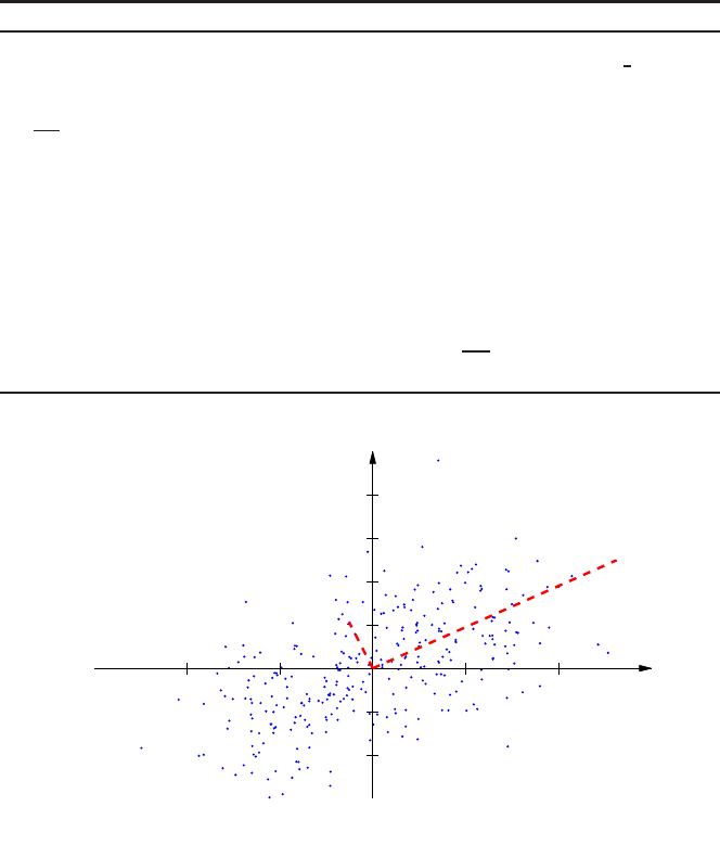
Figure 2 shows the PCA analysis to a two-dimensional point cloud generated by

a combination of Gaussians. After the data is centered, the principal components

are obtained and denoted by u

and u

. Note that the length of the new coordinates

is relative to the energy contained in their eigenvectors. Therefore, for the partic-

ular example depicted in Fig

2, the ﬁrst component u

accounts for 83.5% of the

energy, which means that removing the second component u

would imply losing

only 16.5% of the information.

The rule of thumb is to choose m

′

so that the cumulative energy is above a certain

threshold, typically 90%. PCA allows us to retrieve the original data matrix by pro-

jecting the data onto the new coordinate system X

′

n×m

′

= X

n×m

′

m× m

′

. The new

data matrix X

′

contains most of the information of the original X with a dimension-

ality reduction of m− m

′

Although PCA is a powerful technique, it does have important limitations. PCA

relies on the empirical data set to be a linear combination of a certain basis. For non-

8 Xavier Amatriain, Alejandro Jaimes, Nuria Oliver, and Josep M. Pujol

Algorithm 1 PCA algorithm

1: Substract the mean. For PCA to work properly, the mean of each of the data dimensions must

be zero. Thus the mean is subtracted from each attribute (column): A

. j

= A

. j

−

∑

,∀ j ∈

{1..m}

2: Covariance matrix. Compute the covariance matrix of data A, centered at the origin as C =

n−1

A. The covariance matrix C will be a square matrix of dimensionality m.

3: Calculate Eigenvectors and Eigenvalues. Compute the matrix V of eigenvectors which diag-

onalize the covariance matrix C as V

−1

CV = D, where V contains the eigenvector and the

diagonal of D contains the eigenvalues ({

...

}).

4: Rearrange eigenvectors and eigenvalues. Once the eigenvectors are computed – which are the

principal components of the analysis, they are sorted in decreasing value of their eigenval-

ues and arranged in a matrix W of dimensionality m: The ﬁrst principal component – which

captures most of the data variation – is the eigenvector with the highest eigenvalue.

5: Compress the data. The dimensionality of the principal component matrix W can be reduced

by keeping only the ﬁrst m

′

eigenvectors (W

′

). The loss of information by discarding an eigen-

vector j is the fraction of the eigenvector’s energy that is

∑

, where

is the eigenvalue of

the j-th eigenvector.

−4 −2 2 4

−2

−1

Fig. 2: PCA analysis of a two-dimensional point cloud from a combination of Gaus-

sians. The principal components derived using PCS are u

and u

, whose length is

relative to the energy contained in the components.

Data Mining Methods for Recommender Systems 9

linear data, generalizations of PCA have been proposed, such as Kernel PCA [?].

Another important assumption of PCA is that the original data set has been drawn

from a Gaussian distribution. When this assumption does not hold true, as it is the

case of multi-modal Gaussian or non-Gaussian distributions, there is no warranty

that the principal components are meaningful.

2.3.2 Singular Value Decomposition

Singular Value Decomposition [34] is a powerful technique for dimensionality re-

duction that is related to PCA. The key issue in an SVD decomposition is to ﬁnd a

lower dimensional feature space where the new features represent “concepts” and

the strength of each concept in the context of the collection is computable. Be-

cause SVD allows to automatically derive semantic “concepts” in a low dimensional

space, it is the basis of latent-semantic analysis [57], a very popular technique for

text classiﬁcation in Information Retrieval .

The core of the SVD algorithm lies in the followingtheorem: It is always possible

to decompose a given matrix A into A = U

. Given the n × m matrix data A (n

items, m features), we can obtain an n× r matrix U (n items, r concepts), an r × r

diagonal matrix

(strength of each concept), and an m× r matrix V (m features, r

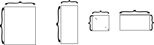
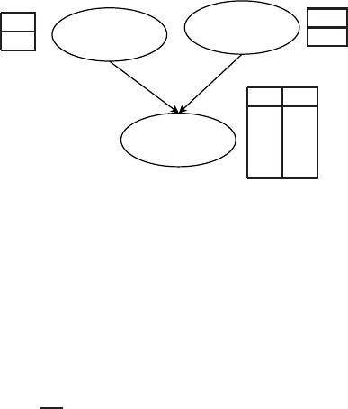
concepts). Figure 3 illustrates this idea.

(items)

(features)

(concepts)

(items)

(features)

(concepts)

Fig. 3: Illustrating the basic Singular Value Decomposition Theorem: an item ×

features matrix can be decomposed into three different ones: an item × concepts, a

concept strength, and a concept × features.

The

diagonalmatrix contains the singular values, which will always be positive

and sorted in decreasing order. The U matrix is interpreted as the “item-to-concept”

similarity matrix, while the V matrix is the “term-to-concept” similarity matrix.

In order to compute the SVD of a rectangular matrix A, we consider AA

and

A. The columns of U are the eigenvectors of AA

, and the columns of V are

the eigenvectors of A

A. The singular values on the diagonal of

are the positive

square roots of the nonzero eigenvalues of both AA

and A

A. Therefore, in order

to compute the SVD of matrix A we ﬁrst compute T as AA

and D as A

A and then

compute the eigenvectors and eigenvalues for T and D.

10 Xavier Amatriain, Alejandro Jaimes, Nuria Oliver, and Josep M. Pujol

The r eigenvalues in

are ordered in decreasing magnitude. Therefore, the orig-

inal matrix A can be approximated by simply truncating the eigenvalues at a given k.

The truncated SVD creates a rank-k approximation to A so that A

= U

. A

the closest rank-k matrix to A. The term “closest” means that A

minimizes the sum

of the squares of the differences of the elements of A and A

. The truncated SVD is

a representation of the underlying latent structure in a reduced k-dimensional space,

which generally means that the noise in the features is reduced.

2.3.3 Dimensionality Reduction in Recommender Systems

Sparsity and the curse of dimensionality are recurring problems in Recommender

Systems. Even in the simplest setting, we are likely to have a sparse matrix with

thousands of rows and columns (i.e. users and items), most of which are zeros.

Therefore, dimensionality reduction comes in naturally. Applying dimensionality

reduction makes such a difference and its results are so directly applicable to the

computation of the predicted value, that this is now considered to be an approach to

Recommender Systems design, rather than a preprocessing technique. As a matter

of fact, the twopreferred approaches to collaborativeﬁltering are nowadays standard

kNN and its many variations, and dimensionality reduction via SVD [].

Earlier works, however, used PCA as a way to reduce dimensionality in a col-

laborative ﬁltering setting. Goldberg et al. proposed an approach to use PCA in the

context of an online joke recommendation system [33]. Their system, known as

Eigentaste

, starts from a standard matrix of user ratings to items. They then select

their gauge set by choosing the subset of items for which all users had a rating. This

new matrix is then used to compute the global correlation matrix where a standard

2-dimensional PCA is applied.

The use of SVD as tool to improve collaborative ﬁltering has been known for

some time. Sarwar et al. [60] describe two different ways to use SVD in this context.

First, SVD can be used to uncover latent relations between customers and products.

In order to accomplish this goal, they ﬁrst ﬁll the zeros in the user-item matrix

with the item average rating and then normalize by subtracting the user average.

This matrix is then factored using SVD and the resulting decomposition can be

used – after some trivial operations – directly to compute the predictions. The other

approach is to use the low-dimensional space resulting from the SVD to improve

neighborhood formation for later use in a kNN approach.

As described by Sarwar et al. [59], one of the big advantages of SVD is that

there are incremental algorithms to compute an approximated decomposition. This

allows to accept new users or ratings without having to recompute the model that

had been built from previously existing data. The same idea was later extended and

formalized by Brand [11] into an online SVD model. The use of incremental SVD

methods has recently become a commonly accepted approach after its success in

http://eigentaste.berkeley.edu

Data Mining Methods for Recommender Systems 11

the Netﬂix Prize

. The publication of Simon Funk’s simpliﬁed incremental SVD

method [31] marked an inﬂection point in the contest. Since its publication, several

improvements to SVD have been proposed in this same context (see Paterek’s en-

sembles of SVD methods [50] or Kurucz et al. evaluation of SVD parameters [43]).

Finally, it should be noted that different variants of Matrix Factorization (MF)

methods such as the Non-negative Matrix Factorization (NNMF) have also been

used [67]. These algorithms are, in essence, similar to SVD. The basic idea is to

decompose the ratings matrix into two matrices, one of which contains features

that describe the users and the other contains features describing the items. Matrix

Factorization methods are better than SVD at handling the missing values by in-

troducing a bias term to the model. However, this can also be handled in the SVD

preprocessing step by replacing zeroes with the item average. Note that both SVD

and MF are prone to overﬁtting. However, there exist MF variants, such as the Regu-

larized Kernel Matrix Factorization [], that can avoid the issue efﬁciently. The main

issue with MF – and SVD – methods is that it is unpractical to recompute the fac-

torization every time the matrix is updated because of computational complexity.

However, Rendle and Schmidt-Thieme [56] propose an online method that allows

to update the factorized approximation without recomputing the entire model.

3 Classiﬁcation

A classiﬁer is a mapping between a feature space and a label space, where the fea-

tures represent characteristics of the elements to classify and the labels represent the

classes. A restaurant recommender system, for example, can be implemented by a

classiﬁer that classiﬁes restaurants into one of two categories (good, bad) based on

a number of features that describe it (e.g., quality of food on a scale from 1 to 10,

atmosphere on a scale from 1 to 10, etc.). A particular restaurant R will be repre-

sented by a feature vector FV

=< fv

, fv

,, fv

>. In this particular example, the

classiﬁer is binary because it produces only two labels: good or bad.

There are many types of classiﬁers, but in general they will either be supervised

or unsupervised.

• In supervised classiﬁcation, a set of labels or categories is knownin advance (e.g.,

we know there are two types of restaurants, good and bad) and we have a set of

labeled examples which constitute a training set (we know in advance which

restaurants are good and which are bad). The task is then to learn a mapping

(boundary, or function) that can separate the instances (good from bad restau-

rants) so that if a new unseen instance (restaurant) is presented to the classiﬁer it

can predict its category (good, bad).

• In unsupervised classiﬁcation, the labels or categories are unknown in advance

and the task is to suitably (according to some criteria) organize the elements at

hand (e.g., given a list of restaurants, put them into groups considering all or

http://www.netﬂixprize.com

12 Xavier Amatriain, Alejandro Jaimes, Nuria Oliver, and Josep M. Pujol

some of their characteristics: quality of food, price, location, etc.). Following

this example, an unsupervised learning algorithm might discover two groups of

restaurants in a list where it might turn out that one group has only French restau-

rants and the other one only American restaurants although the labels “French”

and “American” did not exist in the feature vectors. Unsupervised classiﬁcation

is accomplished by means of clustering algorithms, which will be covered in

section 4.

In essence, then, classiﬁers try to ﬁnd boundary functions to separate or group

elements into either known categories or into groups of similar elements. In this

section we describe several algorithms to learn supervised classiﬁers and will be

covering unsupervised classiﬁcation in section

3.1 Nearest Neighbors

Instance-based classiﬁers work by storing training records and using them to predict

the class label of unseen cases. A trivial example is the so-called rote-learner. This

classiﬁer memorizes the entire training set and classiﬁes only if the attributes of the

new record match one of the training examples exactly.

A more elaborate, and far more popular, instance-based classiﬁer is the Nearest

neighbor classiﬁer (kNN) [19]. Given a point to be classiﬁed, the kNN classiﬁer

ﬁnds the k closest points (nearest neighbors) from the training records. It then as-

signs the class label according to the class labels of its nearest-neighbors. The un-

derlying idea is that if a record falls in a particular neighborhood where a class label

is predominant it is because the record is likely to belong to that very same class.

Given a query point q for which we want to know its class l, and a training

set X = {{x

}...{x

}}, where x

is the j-th element and l

is its class label, the

k-nearest neighbors will ﬁnd a subset Y = {{y

}...{y

}} such that Y ∈ X and

∑

d(q,y

) is minimal. Y contains the k points in X which are closest to the query

point q. Then, the class label of q is l = f({l

...l

}).

The distance measure d is usually the Euclidian distance. However, other mea-

sures, such as the ones reviewed in

2.1, can be applied depending on the data. In

order to prevent the distance measure from being dominated by some of the at-

tributes, it is common-practice to scale attributes. Furthermore, and in order to avoid

counter-intuitive results, we sometimes normalize vectors to unit length.

There are different candidates for the function f by which the new class label is

assigned. The most widely used is the majority vote rule with ties broken at random.

With majority vote, the query point q is assigned to the most common label of its

nearest neighbors. A variation of the majority vote is to weight the votes according

to the distance between the training points y

and the query point q; the vote of the

closest neighbor counts more than the vote of the furthest – this is one of preferred

approach when using kNN in a collaborative ﬁltering setting. Another strategy is

to use the consensus rule. Unlike the majority vote rule, consensus only assigns the

label if and only if all k neighbors have the same class label. This technique is useful

Data Mining Methods for Recommender Systems 13

−3 −2 −1 0 1 2 3

−3

−2

−1

items of cluster 1

items of cluster 2

item to classify

−3 −2 −1 0 1 2 3

−3

−2

−1

items of cluster 1

items of cluster 2

item to classify

Fig. 4: Example of k-Nearest Neighbors. The left subﬁgure shows the training points

with two class labels (circles and squares) and the query point (as a triangle). The

right sub-ﬁgure illustrates closest neighborhood for k = 1 and k = 7. The query

point would be classiﬁed as square for k = 1, and as a circle for k = 5 according to

the simple majority vote rule. Note that the query points was just on the boundary

between the two clusters.

to discriminate the classiﬁcation in terms of certainty, however, many query points

might remain unclassiﬁed due to the strictiveness of this criterium.

Perhaps the most challenging issue in kNN is how to choose the value of k. If k

is too small, the classiﬁer will be sensitive to noise points. But if k is too large, the

neighborhood might include too many points from other classes. The right plot in

Fig.

4 shows how different k yields different class label for the query point, if k = 1

the class label would be circle whereas k = 7 classiﬁes it as square. Note that the

query point from the example is on the boundary of two cluster, and therefore, it is

difﬁcult to classify.

kNN classiﬁers are amongst the simplest of all machine learning algorithms.

Since kNN does not build models explicitly it is considered a lazy learner. Unlike

eager learners such as decision trees or rule-based systems, kNN classiﬁers leave

many decisions to the classiﬁcation step. Therefore, classifying unknown records is

relatively expensive.

3.1.1 Nearest Neighbors in Recommender Systems

Nearest Neighbor is one of the most common approaches to collaborative ﬁlter-

ing (and therefore to designing a recommender systems). As a matter of fact, any

overviewon Recommender Systems – such as the one by Adomavicius and Tuzhilin

[1] – will include an introduction to the use of nearest neighbors in this context.

One of the advantages of this classiﬁer is that it is conceptually very much related

to the idea of collaborative ﬁltering: Finding like-minded users (or similar items) is

essentially equivalent to ﬁnding neighbors for a given user or an item.

14 Xavier Amatriain, Alejandro Jaimes, Nuria Oliver, and Josep M. Pujol

The other advantage is that, being the kNN classiﬁer a lazy learner, it does not

require to learn and maintain a given model. Therefore, in principle, the system can

adapt to rapid changes in the user ratings matrix. Unfortunately, this comes at the

cost of recomputing the neighborhoods and therefore the similarity matrix.

The kNN approach, although simple and intuitive, has shown good accuracy re-

sults and is very amenable to improvements. As a matter of fact, its supremacy as

the de facto standard for collaborative ﬁltering recommendation has only been chal-

lenged recently by approaches based on dimensionality reduction such as the ones

reviewed in Section

2.3.

The general kNN approach to collaborative ﬁltering has experienced improve-

ments in several directions. For instance, in the context of the Netﬂix Prize, Bell

and Koren [7] propose a method to remove global effects such as the fact that some

items may attract users that consistently rate lower. They also propose an optimiza-

tion method for computing interpolating weights once the neighborhood is created.

3.2 Decision Trees

Decision trees [55] are classiﬁers on a target attribute (or class) in the form of a

tree structure. The observations (or items) to classify are composed of attributes and

their target value. The nodes of the tree can be: a) decision nodes, in these nodes a

single attribute-value is tested to determine to which branch of the subtree applies.

Or b) leaf nodes which indicate the value of the target attribute.

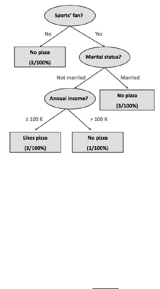
Figure

5 is a decision tree of the data contained in Table 1. In this toy example,

the goal is to classify potential pizza-lovers as a function of three attributes (marital

status, annual income and interest in sports). The tree will then be used to predict

the risk of future borrowers based on historic data.

sub:similarity

Sports’ fan Marital Status Annual income Likes Pizza

Yes Divorced 90K Yes

No Single 125K No

Yes Married 100K No

Yes Married 60K No

Yes Married 75K No

Yes Single 105K No

Yes Single 85K Yes

Yes Single 90K Yes

No Divorced 220K No

No Married 120K No

Table 1: Attributes and target attribute from the observations

There are many algorithms for decision tree induction: Hunts Algorithm, CART,

ID3, C4.5, SLIQ, SPRINT to mention the most common. We brieﬂy describe Hunt’s

Data Mining Methods for Recommender Systems 15

Fig. 5: Example of a Decision Tree for the data summarized in Table 1

Algorithm – used in the toy example – for it is one of the earliest and easiest to

understand. The recursive Hunt algorithm is described in Listing

The algorithm relies on the test condition applied to a given attribute that dis-

criminates the observations by their target values. Once the partition induced by the

test condition has been found, the algorithm is recursively repeated until a partition

is empty or all the observations have the same target value. In Fig.

5 there are three

test conditions, one for each attributed in the data. The ﬁrst test condition was to

ask for sport’s supporters since there is no observation of a non sports’s fan liking

pizza. Applying the condition will create the split of the data in two new nodes: a)

non sports’ fans with three instances and b) sports’ fans with seven instances. Why

was sports chosen to do the split instead of another attribute? Because the partition

yielded by sports maximized the information gain, deﬁned as follows,

∆

= I(parent) −

∑

j=1

N(v

)I(v

)

(9)

where k

are values of the attribute i, N is the number of observations, v

is the

j-th partition of the observations according to the values of attribute i. Finally, I

is a function that measures node impurity. There are different measures of impu-

16 Xavier Amatriain, Alejandro Jaimes, Nuria Oliver, and Josep M. Pujol

Algorithm 2 Hunt algorithm

1: D

= {(X

,..., X

),∀i ∈ N}

2: (the N observations to classify in D

is the target attribute of the i-th instance or observation)

3: c (the current node)

5: procedure Hunt(D

, c)

7: if same value for all Y

in D

then

8: mark c as leaf node with value Y

9: else

10: use test condition to split D

in Q different sets of observations D

..D

11: according the values of an attribute j X

12: for i ∈ Q do

13: Hunt(D

i,i)

14: end for

15: end if

16:

17: end procedure

rity: Gini Index, Entropy and misclassiﬁcation error are the most common in the

literature. We used misclassiﬁcation to build up the example depicted in Fig. 5. We

computed the information

∆

for each attribute and selected sports since it maxi-

mized the information gain. Then, the original observations are split into two new

nodes and the process is repeated.

Note that the test condition selection process uses a greedy hill-climbing strategy.

Decision trees can, therefore, get stuck in a local optimal classiﬁcation. The test

condition is also sensitive to the attribute type (i.e. nominal, ordinal, continuous...)

and whether we decide to do a 2-way split or a multi-way split. However, these

two issues are not uncorrelated. For instance, if we base our partition on nominal

attributes we will favor a multi-way split using as many partitions as distinct values.

We have different ways to handle splitting conditions based on continuousattributes.

We can discretize any continuous attribute to form an ordinal attribute following

either a static or dynamic approach. In the static, we discretize the attribute once

at the beginning. In the dynamic, ranges can be found by equal interval bucketing,

equal frequency bucketing, or clustering.

We already mentioned that the decision tree stops once all observations belong to

the same class (or the same range in the case of continuous attributes). This implies

that the impurity of the leaf nodes is zero. For practical reasons, however, most

decision trees implementations use pruning by which a node is no further split if

its impurity measure or the number of observations in the node are below a certain

threshold. This early termination criteria are used to improve the efﬁciency of the

algorithm. Early termination avoids too ﬁne-grained splits that might be irrelevant

in the prediction stage or could be over-ﬁtting to the training data.

The main advantages of building a classiﬁer using a decision tree is that it is

inexpensive to construct and it is extremely fast at classifying unknown instances.

Data Mining Methods for Recommender Systems 17

Another appreciated aspect of decision tree is that they can be used to produce a set

of rules that are easy to interpret (see section

3.3) while maintaining an accuracy

comparable to other basic classiﬁcation techniques.

3.2.1 Decision Trees in Recommender Systems

Decision trees may be used in a model-based approach for a recommender system.

One possibility is to use content features to build a decision tree that models all the

variables involved in the user preferences. Bouza et al. [9] use this idea to construct

a Decision Tree using semantic information available for the items. The tree is built

after the user has rated only two items. The features for each of the items are used to

build a model that explains the user ratings. They use the information gain of every

feature as the splitting criteria. It should be noted that although this approach is

interesting from a theoretical perspective, the precision they report on their system

is worse than that of recommending the average rating.

As it could be expected, it is very difﬁcult and unpractical to build a decision

tree that tries to explain all the variables involved in the decision making process.

Decision trees, however, may also be used in order to model a particular part of

the system. Cho et al. [14], for instance, present a Recommender System for online

purchases that combines the use of Association Rules (see Section

5) and Decision

Trees. The Decision Tree is used as a ﬁlter to select which users should be targeted

with recommendations. In order to build the model they create a candidate user set

by selecting those users that have chosen products from a given category during

a given time frame. In their case, the dependent variable for building the decision

tree is chosen as whether the customer is likely to buy new products in that same

category.

3.3 Ruled-based Classiﬁers

Rule-based classiﬁers classify data by using a collection of “if .. . then .. .” rules.

The rule antecedent or condition is an expression made of attribute conjunctions.

The rule consequent is a positive or negative classiﬁcation.

We say that a rule r covers a given instance x if the attributes of the instance

satisfy the rule condition. We deﬁne the coverage of a rule as the fraction of records

that satisfy its antecedent. On the other hand, we deﬁne its accuracy as the fraction

of records that satisfy both the antecedent and the consequent. We say that a clas-

siﬁer contains mutually exclusive rules if the rules are independent of each other –

i.e. every record is covered by at most one rule. Finally we say that the classiﬁer has

exhaustive rules if they account for every possible combination of attribute values

–i.e. each record is covered by at least one rule.

In order to build a rule-based classiﬁer we can follow a direct method to extract

rules directly from data. Examples of such methods are RIPPER, or CN2. On the

18 Xavier Amatriain, Alejandro Jaimes, Nuria Oliver, and Josep M. Pujol

other hand, it is common to follow an indirect method and extract rules from other

classiﬁcation models such as decision trees or neural networks.

For instance the rules derived from applying a decision tree

5 to the data of Table

1 would be:

1. IF NOT Sports’ fan THEN NOT Pizza (coverage 30%, accuracy 100%)

2. IF Sports’ fan AND Married THEN NOT Pizza (coverage30%, accuracy 100%)

3. IF Sports’ fan AND NOT Married THEN Pizza (coverage 40%, accuracy 75%)

Note that we excluded the annual income attribute for the sake of illustrating the

coverage and accuracy. The advantages of rule-based classiﬁers are that they are

extremely expressive since they are symbolic and operate with the attributes of the

data without any transformation. Rule-based classiﬁers, and by extension decision

trees, are easy to interpret, easy to generate and they can classify new instances

efﬁciently.

3.3.1 Rule-based Classiﬁers in Recommender Systems

In a similar way to Decision Tress, it is very difﬁcult to build a complete recom-

mender model based on rules. As a matter of fact, this method is not very popular

in the context of recommender systems because deriving a rule-based system means

that we either have some explicit prior knowledge of the decision making process

or that we derive the rules from another model such a decision tree. However a rule-

based dystem can be used to improve the performance of a recommender system by

injecting partial domain knowledge or business rules.

Anderson et al. [3], for instance, implemented a collaborative ﬁltering music

recommender system that improvesits performanceby applying a rule-based system

to the results of the collaborativeﬁltering process. If a user rates an album by a given

artist high, for instance, predicted ratings for all other albums by this artist will be

increased.

Gutta et al. [26] implemented a rule-based recommender system for TV content.

In order to do, so they ﬁrst derived a C4.5 Decision Tree that is then decomposed

into rules for classifying the programs.

Basu et al. [5] followed an inductive approach using the Ripper [16] system to

learn rules from data. They report slightly better results when using hybrid con-

tent and collaborative data to learn rules than when following a pure collaborative

ﬁltering approach.

3.4 Bayesian Classiﬁers

A Bayes classiﬁer [30] is a probabilistic framework for solving classiﬁcation prob-

lems. It is based on the deﬁnition of conditional probability and the Bayes theorem.

The Bayesian school of statistics uses probability to represent uncertainty about the

Data Mining Methods for Recommender Systems 19

relationships learned from the data. In addition, the concept of priors is very im-

portant as they represent our expectations or prior knowledge about what the true

relationship might be. In particular, the probability of a model given the data (pos-

terior) is proportional to the product of the likelihood times the prior probability

(or prior). The likelihood component includes the effect of the data while the prior

speciﬁes the belief in the model before the data was observed.

Bayesian classiﬁers make use of Bayes’ theorem, that relates all the previous

concpts, and is given by:

P(M|D) =

P(D|M)P(M)

P(D)

(10)

where M is a model (or hypothesis) and D is the data. P(M) is the prior probability

of M, i.e. the probability that M is correct before the data D is observed; P(D|M)

is the conditional probability of seeing data D given that model M is true. This is

called the likelihood of the data; P(D) is the marginal probability of the data and

P(M|D) is the posterior probability, i.e. the probability that model M is true, given

the data.

If we assume an exhaustive set of mutually exclusive models M

, we obtain:

P(D) =

∑

P(D,M

) =

∑

P(D|M

)P(M

) (11)

Note that P(D) in Equation

10 is a normalizing constant that only depends on the

data and in most cases does not need to be computed explicitly. As a result, Bayes’

theorem is typically simpliﬁed to P(M|D) ∝ P(D|M)P(M).

Bayesian classiﬁers consider each attribute and class label as (continuous or dis-

crete) random variables. Given a record with N attributes (A

,...,A

), the goal is

to predict class C

by ﬁnding the value ofC

that maximizes the posterior probability

of the class given the data P(C

,...,A

). Applying Bayes’ theorem,

P(C

,...,A

) ∝ P(A

,...,A

)P(C

) (12)

A particular but very common Bayesian classiﬁer is the Naive Bayes Classiﬁer.

In order to estimate the conditional probability, P(A

,...,A

), a Naive Bayes

Classiﬁer assumes the probabilistic independence of the attributes – i.e. the presence

or absence of a particular attribute is unrelated to the presence or absence of any

other. This assumption leads to

P(A

,...,A

) = P(A

)P(A

)...P(A

) (13)

If conditional probabilities are zero, then the entire expression becomes zero so

the Naive Bayes Classiﬁer will not be able to classify the instance. In this case, we

can use the m-estimate approach for estimating conditional probabilities:

P(A

) =

+ mp

n+ m

(14)

20 Xavier Amatriain, Alejandro Jaimes, Nuria Oliver, and Josep M. Pujol

Watches

Sport

(S)

Married

(M)

Likes

Pizza

(P)

P(S)

0.6

P(M)

0.2

S M P(P)

T T 0.8

T F 0.9

F T 0.3

F F 0.4

Fig. 6: Example of a Bayesian Belief Network

where n is the number of training instances in class C, n

is the number of training

instances belonging to class C with attribute A

, p is the prior estimation of the

probability (usually set to one over the number of values of the attribute we are

considering), and m is a parameter known as the equivalent sample size.

Another issue with Bayesian classiﬁers is that the computation of each P(A

)

depends on the nature of the attribute that we are dealing with. In the case of discrete

attributes, P(A

) =

, where |A

| is number of instances that have attribute A

and belong to class C

. Continuous attributes are typically discretized.

The main beneﬁts of Naive Bayes classiﬁers are that they are robust to isolated

noise points and irrelevant attributes, and they handle missing values by ignoring

the instance during probability estimate calculations.

However, the independence assumption may not hold for some attributes as they

might be correlated. In this case, the usual approach is to use the so-called Bayesian

Belief Networks (BBN) (or Bayesian Networks, for short). BBN’s use an acyclic

graph to encode the dependence between attributes and a probability table that as-

sociates each node to its immediate parents (see Fig.

6). If a node A does not have

any parent, the table contains only prior probability P(A); if the node has only one

parent B, the table contains the conditional probability P(A|B); and if the node has

multiple parents, the table contains the conditional probability P(A|B

,...,B

BBN’s provide a way to capture prior knowledge in a domain using a graphical

model. And, although constructing the model is non-trivial, once the structure of

the network is determined it is quite easy to add a new variable. In a similar way

to Naive Bayes classiﬁers, BBN’s handle incomplete data well and they are quite

robust to model overﬁtting.

3.4.1 Bayesian Classiﬁers in Recommender Systems

Bayesian classiﬁers are particularly popular for model-based recommendersystems.

They are often used to derive a model for content-based recommender systems.

However, they have also been used in a collaborative ﬁltering setting.

Data Mining Methods for Recommender Systems 21

Ghani and Fano [32], for instance, use a Naive Bayes classiﬁer to implement a

content-based recommender system. The use of this model allows for recommend-

ing products from unrelated categories in the context of a department store.

Miyahara and Pazzani [48] implement a recommender system based on a Naive

Bayes classiﬁer. In order to do so, they deﬁne two classes: like and don’t like. In this

context they propose two ways of using the Naive Bayesian Classiﬁer: The Trans-

formed Data Model assumes that all features are completely independent, and fea-

ture selection is implemented as a preprocessing step. On the other hand, the Sparse

Data Model assumes that only known features are informative for classiﬁcation.

Furthermore, it only makes use of data which both users rated in common when

estimating probabilities. Experiments show both models to perform better than a

correlation-based collaborative ﬁltering.

Pronk et al. [52] use a Bayesian Naive Classiﬁer as the base for incorporating

user control and improving performance, especially in cold-start situations. In order

to do so they propose to maintain two proﬁles for each user: one learned from the

rating history, and the other explicitly created by the user. The blending of both

classiﬁers can be controlled in such a way that the user-deﬁned proﬁle is favored

at early stages, when there is not too much rating history, and the learned classiﬁer

takes over at later stages.

In the previous section we mentioned that Gutta et al. [26] implemented a rule-

based approach in a TV content recommender system. Another of the approaches

they tested was a Bayesian classiﬁer. They deﬁne a two-class classiﬁer, where the

classes are watched/not watched. The user proﬁle is then a collection of attributes

together with the number of times they occur in positive and negative examples.

This is used to compute prior probabilities that a show belongs to a particular class

and the conditional probability that a given feature will be present if a show is either

positive or negative. It must be noted that features are, in this case, related to both

content –i.e. genre – and contexts –i.e. time of the day. The posteriori probabilities

for a new show are then computed from these.

Breese et al. [12] implement a Bayesian Network where each node corresponds

to each item. The states correspond to each possible vote value. In the network, each

item will have a set of parent items that are its best predictors. The conditional prob-

ability tables are represented by decision trees. The authors report better results for

this model than for several nearest-neighbors implementations over several datasets.

Hierarchical Bayesian Networks have also been used in several settings as a way

to add domain-knowledge for information ﬁltering [71]. One of the issues with hier-

archical Bayesian networks, however, is that it is very expensive to learn and update

the model when there are many users in it. Zhang and Koren [72] propose a varia-

tion over the standard Expectation-Maximization (EM) model in order to speed up

this process in the scenario of a content-based recommender system.

22 Xavier Amatriain, Alejandro Jaimes, Nuria Oliver, and Josep M. Pujol

3.5 Artiﬁcial Neural Networks

The Artiﬁcial Neural Network (ANN) model [74] is an assembly of inter-connected

nodes and weighted links that is inspired in the architecture of the biological brain.

Nodes in an ANN are called neurons as an analogy with biological neurons. These

simple functional units are composed into networks that have the ability to learn a

classiﬁcation problem after they are trained with sufﬁcient data.

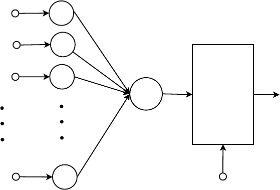
The simplest case of an ANN is the perceptron model, illustrated in ﬁgure

Input Signals

Synaptic Weights

Summing Junction

Activation

Function

Output

Threshold

∑

(•)

Fig. 7: Perceptron model

If we particularize the activation function

to be the simple Threshold Function

, the output is obtained by summing up each of its input value according to the

weights of its links and comparing its output against some threshold

. The output

function can be expressed using Eq.

15. The perceptron model is a linear classiﬁer

that has a simple and efﬁcient learning algorithm summarized in Listing 3.

(

1, if

∑

≥

0, if

∑

(15)

Besides the simple Threshold Function used in the Perceptron model, there are

several other common choices for the activation function such as sigmoid, tanh, or

step functions.

Using neurons as atomic functional units, there are many possible architectures

to put them together in a network. But, by far, the most common approach is to use

Data Mining Methods for Recommender Systems 23

Algorithm 3 Perceptron Learning algorithm

1: Let D = (x

)|i = 1, 2,·· · , N be the set of training examples

2: Initialize the weight vector with random values, w

3: repeat

4: for each training example (x

) ∈ D do do

5: Compute the predicted output ˆy

6: for each weight w

7: Update the weight w

k+1

= w

− ˆy

8: end for

9: end for

10: until stopping condition is met

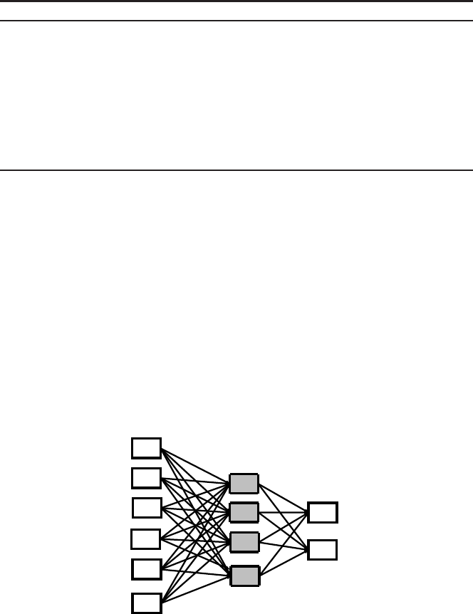
the feed-forward ANN (see ﬁgure 8). In this case, signals are strictly progated in one

way: from input to output.

An ANN can have any number of layers. The simple feedforward network in ﬁg-

ure

8 has three layers. On the other hand, the perceptron in ﬁgure 7 is a single-layer

feed-forward ANN. Layers in an ANN are classiﬁed into three types: input, hidden,

and output. Units in the input layer respond to data that is fed into the network.

Hidden units receive the weighted output from the input units. And the output units

respond to the weighted output from the hidden units and generate the ﬁnal output

of the network.

Feedforward

Neural Net

Input Layer

Output Layer

Hidden Layer

Fig. 8: Example of a simple feed-forward ANN with one hidden layer

The learning algorithm in listing

3 is only valid for the simple Perceptron model.

There exist supervised, unsupervised, and reinforcement learning algorithms for the

general case of multilayer networks. The generic algorithm for learning ANN in a

supervised way, for instance, is summarized in ﬁgure

9. The most common concrete

24 Xavier Amatriain, Alejandro Jaimes, Nuria Oliver, and Josep M. Pujol

algorithm for learning ANN’s is the so-called back-propagation algorithm, based

on the computation of the error derivative of the weights. However, it is beyond the

scope of this chapter to go into the details of this algorithm.

Input Features

Neural

Net

Supervised

Learning

Algorithm

Target Features

Fig. 9: Supervised learning process for learning an ANN

The main advantages of ANN are that – depending on the activation function

– they can perform non-linear classiﬁcation tasks, and that, due to their parallel

nature, they can be efﬁcient and even operate if part of the network fails. The main

disadvantage is that it is hard to come up with the ideal network topology for a

given problem and once the topology is decided this will act as a lower bound for

the classiﬁcation error. ANN’s belong to the class of sub-symbolic classiﬁers, which

means that they provide no semantics for inferring knowledge – i.e. they promote a

kind of black-box approach.

3.5.1 Artiﬁcial Neural Networks in Recommender Systems

ANN’s can be used in a similar way as Bayesian Networks to construct model-based

recommender systems. However, there is no conclusive study to whether ANN in-

troduce any performance gain. As a matter of fact, Pazzani and Billsus [51] did

a comprehensive experimental study on the use of several machine learning algo-

rithms for web site recommendation. Their main goal was to compare the simple

naive Bayesian Classiﬁer with computationally more expensive alternatives such as

Decision Trees and Neural Networks. Their experimental results show that Deci-

sion Trees perform signiﬁcantly worse. On the other hand ANN and the Bayesian

Data Mining Methods for Recommender Systems 25

classiﬁer perform similarly. They conclude that there does not seem to be a need for

nonlinear classiﬁers such as the ANN.

ANN can be used to combine (or hybridize) the input from several recommen-

dation modules or data sources. Hsu et al. [27], for instance, build a TV recom-

mender by importing data from four different sources: user proﬁles and stereotypes;

viewing communities; program metadata; and viewing context. They use the back-

propagation algorithm to train a three-layered neural network.

Berka et al. [28] used ANN to build an URL recommender system for web navi-

gation. They implemented a content-independent system based exclusively on trails

– i.e. associating pairs of domain names with the number of people who traversed

them. In order to do so they used feed-forward Multilayer Perceptrons trained with

the Backpropagation algorithm.

Christakou and Stafylopatis [15] build a hybrid content-based collaborative ﬁl-

tering recommender system. The content-based recommender is implemented using

three neural networks per user, each of them corresponding to one of the following

features: “kinds”, “stars”, and “synopsis”. They trained the ANN using the Resilient

Backpropagation method.

3.6 Support Vector Machines

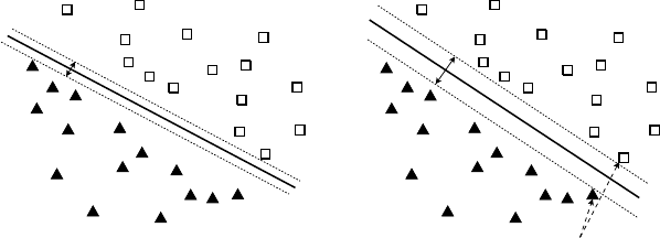
The goal of a Support Vector Machine (SVM) classiﬁer [20] is to ﬁnd a linear hy-

perplane (decision boundary) that separates the data in such a way that the margin is

maximized. For instance, if we look at a two class separation problem in two dimen-

sions like the one illustrated in ﬁgure

10, we can easily observe that there are many

possible boundarylines to separate the two classes. Each boundary has an associated

margin. The rationale behind SVM’s is that if we choose the one that maximizes the

margin we are less likely to missclassify unknown items in the future.

Large Margin

Small Margin

Support Vectors

w• x+ b = 0

w• x+ b = 1

w• x+ b = −1

Fig. 10: Different boundary decisions are possible to separate two classes in two

dimensions. Each boundary has an associated margin.

26 Xavier Amatriain, Alejandro Jaimes, Nuria Oliver, and Josep M. Pujol

A linear separation between two classes is accomplished through the following

function:

w• x+ b = 0 (16)

We deﬁne a function that can classify items of being of class +1 or -1 as long

as they are separated by some minimum distance from the class separation function

previously deﬁned. The function is given by Eq. 17

f(x) =

(

1, if w• x+ b ≥ 1

−1, if w• x+ b ≤ −1

(17)

Margin =

kwk

(18)

Following the main rationale for SVM’s, we would like to maximize the margin

between the two classes, given by equation

18. This is in fact equivalent to mini-

mizing the inverse value L(w) =

kwk

but subjected to the constraints given by f(x).

This is a constrained optimization problem and there are numerical approaches to

solve it (e.g., quadratic programming).

If the items are not linearly separable we can decide to turn the svm into a soft

margin classiﬁer by introducing a slack variable. In this case the formula to mini-

mize is given by equation

19 subject to the new deﬁnition of f(x) in equation 20.

Note that the constant C in equation 19 allows to deﬁne the cost of a constraint

violation.

L(w) =

kwk

∑

i=1

(19)

f(x) =

(

1, if w• x+ b ≥ 1−

−1, if w• x+ b ≤ −1+

(20)

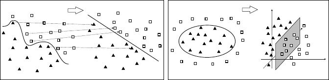
On the other hand, if the decision boundary is not linear we need to transform

data into a higher dimensional space (see ﬁgure

11). This is accomplished thanks

to a mathematical transformation known as the kernel trick. The basic idea is to re-

place the dot products in equation 17 by a kernel function. There are many different

possible choices for the kernel function such as Polynomial or Sigmoid. But by far

the most common kernel function are the family of Radial Basis Function (RBF).

The formulation for a Gaussian RBF, for instance, is given by Eq.

21.

k(x,x

′

) = exp(−

||x− x

′

) (21)

Data Mining Methods for Recommender Systems 27

Input Space

Transformed Feature Space

(a)

Input Space

Transformed Feature Space

(b)

Fig. 11: Mapping input data into a different feature space where problem will be

linearly separable

3.6.1 Support Vector Machines in Recommender Systems

Support Vector Machines have recently gained popularity for their performance and

efﬁciency in many settings. SVM’s have also shown promising recent results in

recommender systems.

Kang and Yoo [42], for instance, report on an experimental study that aims at se-

lecting the best preprocessing technique for predicting missing values for an SVM-

based recommender system. In particular,they use SVD and Support Vector Regres-

sion. The Support Vector Machine recommender system is built by ﬁrst binarizing

the 80 levels of available user preference data. They experiment with several settings

and report best results for a threshold of 32 – i.e. a value of 32 and less is classiﬁed

as prefer and a higher value as do not prefer. The user id is used as the class label

and the positive and negative values are expressed as preference values 1 and 2.

Xu and Araki [69] used SVM to build a TV program recommender system. They

use information from the Electronic Program Guide (EPG) as features. But in order

to reduce features they removed words with lowest frequencies. Furthermore, and

in order to evaluate different approaches, they used both the Boolean and the Term

frequency - inverse document frequency (TFIDF) weighting schemes for features.

In the former, 0 and 1 are used to represent absence or presence of a term on the

content. In the latter, this is turned into the TFIDF numerical value.

Xia et al. [68] present different approaches to using SVM’s for recommendersys-

tems in a collaborative ﬁltering setting. They explore the use of Smoothing Support

Vector Machines (SSVM). They also introduce a SSVM-based heuristic (SSVMBH)

to iteratively estimate missing elements in the user-item matrix. They compute pre-

dictions by creating a classiﬁer for each user. Their experimental results report best

results for the SSVMBH as compared to both SSVM’s and traditional user-based

and item-based collaborative ﬁltering.

Oku et al. [24] propose the use of Context-Aware Vector Machines (C-SVM)

for context-aware recommender systems. They compare the use of standard SVM,

C-SVM and an extension that uses collaborative ﬁltering as well as C-SVM. Their

28 Xavier Amatriain, Alejandro Jaimes, Nuria Oliver, and Josep M. Pujol

results show the effectiveness of the context-aware methods for restaurant recom-

mendations.

3.7 Ensembles of Classiﬁers

The basic idea behind the use of ensembles of classiﬁers is to construct a set of

classiﬁers from the training data and predict class label of previously unseen records

by aggregating their predictions.

Ensembles of classiﬁers work whenever we can assume that the classiﬁers are

independent. In this case we can ensure that the ensemble will produce results that

are in the worst case as bad as the worst classiﬁer in the ensemble. Therefore, com-

bining classiﬁers of a similar classiﬁcation error will only improve results.

In order to generate ensembles, several approaches are possible. The two most

common techniques are Bagging and Boosting. In Bagging, we perform sampling

with replacement, building the classiﬁer on each bootstrap sample. Therefore each

sample has probability (11/n)n of being selected. In Boosting we use an iterative

procedure to adaptively change distribution of training data by focusing more on

previously misclassiﬁed records. Initially, all records are assigned equal weights.

But, unlike bagging, weights may change at the end of each boosting round: Records

that are wrongly classiﬁed will have their weights increased while records that are

classiﬁed correctly will have their weights decreased. An example of boosting is the

AdaBoost algorithm.

3.7.1 Ensembles of Classiﬁers in Recommender Systems

The use of ensembles of classiﬁers is common practice in the recommender sys-

tems ﬁeld. As a matter of fact, any hybridation technique [13] can be considered an

ensemble as it combines in one way or another several classiﬁers.

Experimental results show that ensembles can produce better results than any

classiﬁer in isolation. Bell et al. [8], for instance, used a combination of 107 differ-

ent methods in their progress prize winning solution to the Netﬂix challenge. They

state that their ﬁndings show that it pays off more to ﬁnd substantially different ap-

proaches rather than focusing on reﬁning a particular technique. This is related to

the property we highlighted before: if classiﬁers are uncorrelated, their combination

can only improve results. In order to blend the results from the ensembles they use

a linear regression approach. In order to derive weights for each classiﬁer, they par-

tition the test dataset into 15 different bins and derive unique coefﬁcients for each

of the bins.

Data Mining Methods for Recommender Systems 29

3.8 Evaluating Classiﬁers

Learning algorithms and classiﬁers can be evaluated by multiple criteria. This in-

cludes how accurately they perform the classiﬁcation, their computational complex-

ity during training , complexity during classiﬁcation, their sensitivity to noisy data,

their scalability, and so on. In this section we will focus only on classiﬁcation per-

formance. In order to evaluate a model we usually take into account the following

measures: True Positives (TP): number of instances classiﬁed as belonging to class

A that truly belong to class A; True Negatives (TN): number of instances classiﬁed

as not belonging to class A and that in fact do not belong to class A; False Positives

(FP): number of instances classiﬁed as class A but that do not belong to class A;

False Negatives (FN): instances not classiﬁed as belonging to class v but that in

fact do belong to class A.

The most commonly used measure for model performance is its Accuracy deﬁned

as the ratio between the instances that have been correctly classiﬁed (as belonging

or not to the given class) and the total number of instances.

Accuracy = (TP+ TN)/(TP+ TN + FP+ FN) (22)

However, accuracy might be misleading in many cases. Imagine a 2-class prob-

lem in which there are 99,900 samples of class A and 100 of class B. If a classiﬁer

simply predicts everything to be of class A, the computed accuracy would be of

99.9%. However, the model performance is questionable because it will never de-

tect any class B examples.

One way to improve this evaluation is to deﬁne the cost matrix where we declare

the cost of misclassifying class B examples as being of class A. In real world appli-

cations different types of errors may indeed have very different costs. For example,

if the 100 samples above correspond to defective airplane parts in an assembly line,

incorrectly rejecting a non-defective part (one of the 99,900 samples) has a negli-

gible cost compared to the cost of mistakenly classifying a defective part as a good

part.

Other common measures of model performance, particularly in Information Re-

trieval, are Precision and Recall.

P = TP/(TP + FP) (23)

R = TP/(TP+ FN) (24)

Precision is a measure of how many errors we make in classifying samples as

being of class A. Recall measures how good we are in not leaving out samples that

should have been classiﬁed as belonging to the class. Note that these two measures

are misleading when used in isolation in most cases. We could build a classiﬁer

of perfect precision by not classifying any sample as being of class A (therefore

obtaining 0 TP but also 0 FP). Conversely, we could build a classiﬁer of perfect

recall by classifying all samples as belonging to class A.

30 Xavier Amatriain, Alejandro Jaimes, Nuria Oliver, and Josep M. Pujol

As a matter of fact, there is a measure, called the F

-measure that combines both

Precision and Recall into a single measure as:

2RP

R+ P

2TP

2TP+ FN + FP

(25)

Additional factors that impact performance include the class distribution and the

size of the training and test sets. In order to address changes due to training sampling

size, we can construct the so-called Learning Curve, which shows how accuracy

changes with varying training sample size. This requires to decide on a sampling

strategy in order to create the curve. These sampling strategies were reviewed in

section

2.2

Sometimes we would like to compare several competing models rather than es-

timate their performance independently. In order to do so we use a technique de-

veloped in the 1950s for analysis of noisy signals: the Receiver Operating Charac-

teristic (ROC) Curve. A ROC curve characterizes the relation between positive hits

and false alarms. The performance of each classiﬁer is represented as a point on the

curve (see Fig.

12).

0.2

0.4

0.6

0.8

0 0.2 0.4 0.6 0.8 1

True Positive Rate

False Positive Rate

Model 1

Model 2

Fig. 12: Example of ROC Curve. Model 1 performs better for low False Positive

Rates while Model 2 is fairly consistent throughout and outperforms Model 1 for

False Positive Rates higher than 0.25

Data Mining Methods for Recommender Systems 31

We plot the relation between TP and FP on a two-dimensional plot. Any point

located at x > y is classiﬁed as positive. Some points of interest in a ROC curve are

(TP,FP) = (0, 0): declare everything to be negative class; (1,1): declare everything

to be positive class; (1,0): ideal. The diagonal line means random guessing and

below the diagonal line the prediction is opposite of the true class.

3.8.1 Evaluation of Classiﬁers in Recommender Systems

The most commonly accepted evaluation measure for recommender systems is the

Mean Average Error (MAE) or Root Mean Squared Error (RMSE) of the predicted

interest (or rating) and the measured one. These measures measure accuracy with-

out any assumption on the purpose of the recommender system. However, as Mc-

Nee et al. point out [47], there is much more than accuracy to deciding whether

an item should be recommended. Herlocker et al. [38] provide a comprehensive re-

view of algorithmic evaluation approaches to recommender systems. They suggest

that some measures could potentially be more appropriate for some tasks. However,

they are not able to validate the measures when evaluating the different approaches

empirically on a class of recommendation algorithms and a single set of data.

A step forward is to consider that the purpose of a “real” recommender system

is to produce a top-N list of recommendations and evaluate recommender systems

depending on how well they can classify items as being recommendable. Ziegler et

al. show [73] that evaluating recommender algorithms through top-N lists measures

still does not map directly to the user’s utility function. However, it does address

some of the limitations of the more commonly accepted accuracy measures, such as

MAE.

If we look at our recommendation as a classiﬁcation problem, we can make use

of well-known measures for classiﬁer evaluation such as precision and recall. Basu

et al. [6], for instance, use these measures by analyzing which of the items predicted

in the top quartile of the rating scale were actually evaluated in the top quartile by

the user.

McLaughlin and Herlocker [46] propose a modiﬁed precision measure in which

non-rated items are counted as not recommendable. This precision measure in fact

represents a lower-bound of the “real” precision.

Although the F-measure can be directly derived from the precision-recall values,

it is not common to ﬁnd it in recommender systems evaluations. Huang et al. [39]

and Bozzon et al. [10], and Miyahara and Pazzani [48] are some of the few examples

of the use of this measure.

ROC curves have also been used in evaluating recommender systems. Zhang et

al. [58] use the value of the area under the ROC curve as their evaluation measure

when comparing the performance of different algorithms under attack. Banerjee and

Ramanathan [4] also use the ROC curves to compare the performance of different

models.

It must be noted, though, that the choice of a good evaluation measure, even

in the case of a top-N recommender system, is still a matter of discussion. Many

32 Xavier Amatriain, Alejandro Jaimes, Nuria Oliver, and Josep M. Pujol

authors have proposed measures that are only indirectly related to these traditional

evaluation schemes. Deshpande and Karypis [21], for instance, propose the use of

the hit rate and the average reciprocal hit-rank. On the other hand, Breese et al. [12]

deﬁne a measure of the utility of the recommendation in a ranked list as a function

of the neutral vote.

4 Cluster Analysis

Clustering [37], also referred to as unsupervised learning, consists of assigning

items to groups so that the items in the same groups are more similar than items

in different groups: the goal is to discover natural (or meaningful) groups that ex-

ist in the data. Similarity is determined using a distance measure, such as the ones

reviewed in

2.1, between the feature vectors that represent the items. The goal of a

clustering algorithm is to minimize intra-cluster distances while maximizing inter-

cluster distances because these constitute measures of the quality of a particular

clustering. Intuitively this means that a good clustering of a set of data points shows

clearly distinct groups. Note that in clustering there is no prior knowledge of class

labels (as was the case in supervised learning). For example, a person who has an

mp3 song collection may not have the songs in individualfolders, but a good cluster-

ing algorithm might discover that the collection has mainly 3 groups (which could

correspond, for example, to classical, heavy metal, and folk).

There are two main categories of clustering algorithms: hierarchical and parti-

tional.

• Partitional clustering algorithms divide data items into non-overlapping clusters

such that each data item is in exactly one cluster.

• Hierarchical clustering algorithms successively cluster items within found clus-

ters, producing a set of nested cluster organized as a hierarchical tree.

Features used to represent an item play a crucial role in determining the cluster-

ing, as does the similarity metric used. In addition, items can be assigned member-

ship values within a group (in fuzzy clustering an items membership in a group is

assigned a value, commonly between 0 and 1), and it can be established that items

have to belong to only one group or may belong to several.

Many clustering algorithms try to minimize a function that measures the quality

of the clustering. Such a quality function is often referred to as the objective func-

tion, so clustering can be viewed as an optimization problem: the ideal clustering

algorithm would consider all possible partitions of the data and output the partition-

ing that minimizes the quality function. But the corresponding optimization problem

is NP hard, so many algorithms resort to heuristics (e.g., in the k-means algorithm

using only local optimization procedures potentially ending in local minima). The

main point is that clustering is a difﬁcult problem for which ﬁnding optimal solu-

tions is often not possible.

Data Mining Methods for Recommender Systems 33

Selection of the particular clustering algorithm and its parameters (e.g., similarity

measure) depend on many factors, including the characteristics of the data. In the

following sections we describe the k-means clustering algorithm and some of its

alternatives.

4.1 k-Means

k-Means (also known as k-centers) clustering is a partitioning method. The function

partitions the data set of N items into k disjoint subsets S

that contain N

items so

that they are as close to each other as possible according a given distance measure.

Each cluster in the partition is deﬁned by its members N

and by its centroid

. The

centroid for each cluster is the point to which the sum of distances from all items in

that cluster is minimized. Thus, we can deﬁne the k-means algorithm as an iterative

process to minimize

E =

∑

n∈S

d(x

) (26)

where x

is a vector representing the n-th item,

is the centroid of the item in S

and d is the distance measure. The k-means algorithm moves items between clusters

until E cannot be decreased further. The algorithm is described in Listing

Algorithm 4 k-means

1: Input

2: X = x

,..., x

(items to be clustered)

3: k (number of clusters)

4: Output

,..,

(cluster centroids)

6: m : X → C (cluster membership)

8: Set the centroids

to their initial value (e.g. random selection of k items in X)

10: for x

∈ X do

11: m(x

) = argmin

j∈{1..k}

d(x

) (assign each item to the closest centroid)

12: end for

13:

14: while m has changed do

15: for j ∈ {1..k} do

16: Recalculate the centroid

according to the items that belong to it {i|m(i) = j}

17: end for

18: for x

∈ X do

19: m(x

) = argmin

j∈{1..k}

d(x

) (update the membership of x

to the closest centroid)

20: end for

21: end while

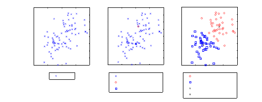
34 Xavier Amatriain, Alejandro Jaimes, Nuria Oliver, and Josep M. Pujol

−4 −2 0 2 4

−4

−3

−2

−1

−4 −2 0 2 4

−4

−3

−2

−1

−4 −2 0 2 4

−4

−3

−2

−1

items

centroid of cluster 1

centroid of cluster 2

items of cluster 1

items of cluster 2

centroid of cluster 1

centroid of cluster 2

Fig. 13: Example of k-means, with k=2. From left to right, the data to be partitioned,

the initial 2 centroids as two data items chosen at random, and ﬁnally, the ﬁnal

partition of the data in 2 clusters (with the centroid of the clusters as ×)

The algorithm works by randomly selecting k centroids. Then all items are as-

signed to the cluster whose centroid is the closest to them. The new cluster centroid

needs to be updated to account for the items who have been added or removed from

the cluster and the membership of the items to the cluster updated. This operation

continues until there are no further items that change their cluster membership. Most

of the convergence to the ﬁnal partition takes place during the ﬁrst iterations of the

algorithm, and therefore, the stopping condition is often changed to “until relatively

few points change clusters” in order to improve efﬁciency.

The distance measure depends on the data we need to cluster. In the example

in ﬁgure

13 we used the sum of square errors (SSE) (d(x

) =

∑

−

)

However, other measures such as the Euclidian distance, Cosine similarity, Pearson

correlation, Manhattan distance or Hamming distance are also widely used.

The basic k-means has several shortcomings: (1) it does assume prior knowl-

edge of the data in order to choose the appropriate k. If the number of clusters is

unknown it is advisable to run the algorithm for a range of k and then choose the

partition whose in which the distance between the items of one cluster with respect

to the items of the rest of the clusters is high. (2) The ﬁnal clusters are very sen-

sitive to the selection of the initial centroids. Thus, different runs of the algorithm

could yield different clusters. To address this issue it has been proposed to run m

replicas with different seeds – the initial centroid – and to return the one with the

lowest value of E. More sophisticated techniques involve data sampling and using

hierarchical clustering to determine the initial centroids. Another technique is to use

the Bisecting k-means, which is a a variant of k-means that can produce a hierar-

chical clustering. The last shortcoming (3) is that the basic k-means can produce

empty clusters, there are several strategies to deal with this issue, from treating it as

an error to treat it as a singleton, creating a new cluster consisting of the one point

furthest from its centroid.

k-means is an extremely simple and efﬁcient algorithm but, apart from the is-

sued just described it does have several limitations with regard to the data. k-means

Data Mining Methods for Recommender Systems 35

has problems when clusters are of differing sizes, densities, non-globular shapes.

k-means also has problems when the data contains outliers.

4.2 Alternatives to k-means

Although the k-means algorithm presents limitations, the truth is that it is very difﬁ-

cult to ﬁnd practical alternatives. In the following paragraphs we will brieﬂy review

some of them.

Density-based clustering algorithms such as DBSCAN work by building up on

the deﬁnition of density as the number of points within a speciﬁed radius. DBSCAN,

for instance, deﬁnes three kinds of points: core points are those that have more than

a speciﬁed number of neighbors within a given distance; border points have fewer

than the speciﬁed number but belong to a core point neighborhood; and noise points

are those that are neither core or border. The algorithm iteratively removes noise

points and performs clustering on the remaining points.

Message-passing clustering algorithms are a very recent family of graph-based

clustering methods. Instead of considering an initial subset of the points as centers

and then iteratively adapt those, message-passing algorithms initially consider all

points as centers – usually known as exemplars in this context. During the algorithm

execution points, which are now considered nodes in a network, exchange messages

until clusters gradually emerge. Afﬁnity Propagation is an important representative

of this family of algorithms [29] that works by deﬁning two kinds of messages

between nodes: “responsibility”, which reﬂects how well-suited receiving point is

to serve as exemplar of the point sending the message, taking into account other

potential exemplars; and “availability”, which is sent from candidate exemplar to the

point and reﬂects how appropriate it would be for the point to choose the candidate

as its exemplar, taking into account support from other points that are choosing that

same exemplar. Afﬁnity propagation has been applied, with very good results, to

problems as different as DNA sequence clustering, face clustering in images, or text

summarization.

Finally, Hierarchical Clustering, produces a set of nested clusters organized as

a hierarchical tree (dendogram). Hierarchical Clustering does not have to assume

a particular number of clusters in advanced. Also, any desired number of clusters

can be obtained by selecting the tree at the proper level. Hierarchical clusters can

also sometimes correspond to meaningful taxonomies. Traditional hierarchical al-

gorithms use a similarity or distance matrix and merge or split one cluster at a time.

There are two main approaches to hierarchical clustering. In agglomerative hier-

archical clustering we start with the points as individual clusters and at each step,

merge the closest pair of clusters until only one cluster (or k clusters) are left. In

divisive hierarchical clustering we start with one, all-inclusive cluster, and at each

step, split a cluster until each cluster contains a point (or there are k clusters).

36 Xavier Amatriain, Alejandro Jaimes, Nuria Oliver, and Josep M. Pujol

4.3 Cluster Analysis in Recommender Systems

The main problem for scaling a collaborative ﬁltering classiﬁer is the amount of op-

erations involved in computing distances – for ﬁnding the best k-nearest neighbors,

for instance. A possible solution is, as we saw in section

2.3, to reduce dimension-

ality. But, even if we reduce dimensionality of features, we might still have many

objects to compute the distance to. This is where clustering algorithms can come

into play. The same is true for content-based recommendersystems, where distances

among objects are needed to retrieve similar ones.

Clustering is sure to improve efﬁciency because the number of operations is re-

duced. However, and unlike dimensionality reduction methods, it is unlikely that it

can help improve accuracy. Therefore, clustering must be applied with care when

designing a recommender system, measuring the compromise between improved

efﬁciency and a possible decrease in accuracy.

We shall now review some known applications of clustering techniques in rec-

ommender systems.

Xue et al. [70] present a typical use of clustering in the context of a recommender

systems by employing the k-means algorithm as a pre-processing step to help in

neighborhood formation. They do not restrict the neighborhood to the cluster the

user belongs to but rather use the distance from the user to different cluster cen-

troids as a pre-selection step for the neighbors. They also implement a cluster-based

smoothing technique in which missing values for users in a cluster are replaced

by cluster representatives. Their method is reported to perform slightly better than

standard kNN-based collaborative ﬁltering.

In a similar way, Sarwar et al. [23] describe an approach to implement a scalable

kNN classiﬁer. They partition the user space by applying the bisecting k-means al-

gorithm and then use those clusters as the base for neighborhood formation. They

report a decrease in accuracy of around 5% as compared to standard kNN CF. How-

ever, their approach allows for a signiﬁcant improvement in efﬁciency.

Connor and Herlocker [18] present a different approach in which, instead of

users, they cluster items. Using the Pearson Correlation similarity measure they try

out four different algorithms: average link hierarchichal agglomerative [35], robust

clustering algorithm for categorical attributes (ROCK) [36], kMetis, and hMetis

Although clustering did improve efﬁciency, all of their clustering techniques yielded

worse accuracy and coverage than the non-partitioned baseline.

Li et al. [54] and Ungar and Foster [63] present a very similar approach for using

k-means clustering for solving a probabilistic model interpretation of the recom-

mender problem.

To the best of our knowledge, alternatives to k-means such as the ones presented

in section

4.2 have not been applied to recommender systems. The simplicity and

efﬁciency of the k-means algorithm shadows possible alternatives. It is not clear

whether density-based or hierarchical clustering approaches have anything to offer

in the recommender systems arena. On the other hand, message-passing algorithms

http://www.cs.umn.edu/ karypis/metis

Data Mining Methods for Recommender Systems 37

have been shown to be more efﬁcient and their graph-based paradigm can be easily

translated to the recommender systems problem. It is possible that we see applica-

tions of these algorithms in the coming years.

5 Association Analysis

Association Rule Mining focuses on ﬁnding rules that will predict the occurrence of

an item based on the occurrences of other items in a transaction. The fact that two

items are found to be related means co-occurrence but not causality.

We deﬁne an itemset as a collection of one or more items (e.g. (Milk, Beer,

Diaper)). A k-itemset is an itemset that contains k items. The frequency of a given

itemset is knownas support count (e.g. (Milk, Beer, Diaper) = 131). And the support

of the itemset is the fraction of transactions that contain it (e.g. (Milk, Beer, Diaper)

= 0.12). A frequent itemset is an itemset with a support that is greater or equal to a

minsup threshold.

An association rule is an expression of the form X ⇒ Y, where X and Y are

itemsets. (e.g. Milk,Diaper ⇒ Beer). In this case the support of the association

rule is the fraction of transactions that have both X and Y. On the other hand, the

conﬁdence of the rule is how often items in Y appear in transactions that contain X.

Given a set of transactions T, the goal of association rule mining is to ﬁnd

all rules having support ≥ minsupthreshold and confidence ≥ minconfthreshold.

The brute-force approach would be to list all possible association rules, compute the

support and conﬁdence for each rule and then prune rules that do not satisfy both

conditions. This is, however, computationally very expensive.

For this reason, we take a two-step approach: (1) Generate all itemsets whose

support ≥ minsup (Frequent Itemset Generation); (2) Generate high conﬁdence

rules from each frequent itemset (Rule Generation)

5.1 Frequent Itemset generation and the Apriori Principle

But if we follow a brute-force approach, frequent itemset generation is still compu-

tationally expensive. Each itemset in the lattice is a candidate frequent itemset and

we have to count the support of each candidate by scanning the transaction database

(i.e. match each transaction against every candidate).

Several techniques exist to optimize the generation of frequent itemsets. On a

broad sense they can be classiﬁed into those that try to minimize the number of

candidates (M), those that reduce the number of transactions (N), and those that

reduce the number of comparisons (NM).

The most common approach though, is to reduce the number of candidates using

the Apriori principle. This principle states that if an itemset is frequent, then all of

its subsets must also be frequent. This is veriﬁed using the support measure because

38 Xavier Amatriain, Alejandro Jaimes, Nuria Oliver, and Josep M. Pujol

the support of an itemset never exceeds that of its subsets. The Apriori Algorithm is

a practical implementation of the principle. Its basic steps are illustrated in listing

Algorithm 5 Apriori algorithm

1: Let k=1

2: Generate frequent itemsets of length 1

3: repeat

4: Generate length (k+1) candidate itemsets from length k frequent itemsets

5: Prune candidate itemsets containing subsets of length k that are infrequent

6: Count the support of each candidate by scanning the DB

7: Eliminate candidates that are infrequent, leaving only those that are frequent

8: until no new frequent itemsets are identiﬁed

Several implementation strategies are also possible to reduce the number of com-

parisons. However, no matter what strategies we adopt, we need to be aware of the

factors that affect computational complexity. First, there is the minimum support

threshold. A lower threshold may produce more and longer frequent itemsets. An-

other factor that affects is the number of items of the data set (dimensionality). More

items means more space to store support count. The size of the transaction database

might also affect algorithms such as the Apriori, which requires multiple passes.

5.2 Rule Generation

Given a frequent itemset L, the goal when generating rules is to ﬁnd all non-empty

subsets that satisfy the minimum conﬁdence requirement.

If |L| = k, then there are 2k2 candidate association rules. So, as in the frequent

itemset generation, we need to ﬁnd ways to generate rules efﬁciently.

For the Apriori Algorithm we can generate candidate rules by merging two rules

that share the same preﬁx in the rule consequent. E.g. join(CD ⇒ AB,BD ⇒ AC)

would produce the candidate rule D ⇒ ABC. We could therefore prune rule D ⇒

ABC provided that its subset AD ⇒ BC does not have high conﬁdence.

5.3 Association Rules in Recommender Systems

The effectiveness of association rule mining for uncovering patterns and driving

personalized marketing decisions has been known for a some time [2]. However,and

although there is a clear relation between this method and the goal of a recommender

system, they have not become mainstream. The main reason is that this approach is

similar to item-based collaborative ﬁltering but is less ﬂexible since it requires of an

explicit notion of transaction – e.g. co-ocurrence of events in a given session. In the

Data Mining Methods for Recommender Systems 39

next paragraphs we present some promising examples, some of which indicate that

association rules still have not had their last word.

Mobasher et al. [49] present a system for web personalization based on associ-

ation rules mining. Their system identiﬁes association rules from pageviews co-

occurrences based on users navigational patterns. Their approach outperforms a

kNN-based recommendation system both in terms of precision and coverage.

Smyth et al. [61] present two different case studies of using association rules for

recommender systems. In the ﬁrst case they use the a priori algorithm to extract item

association rules from user proﬁles in order to derive a better item-item similarity

measure. In the second case, they apply association rule mining to a conversational

recommender. The goal here is to ﬁnd co-occurrent critiques – i.e. user indicating a

preference over a particular feature of the recommended item.

Lin et al. [45] present a new association mining algorithm that adjusts the min-

imum support of the rules during mining in order to obtain an appropriate num-

ber of signiﬁcant rule therefore addressing some of the shortcomings of previ-

ous algorithms such as the a priori. They mine both association rules between

users and items. The measured accuracy outperforms previously reported values for

correlation-based recommendation and is similar to the more elaborate approaches

such as the combination of SVD and ANN.

As already mentioned in section

3.2.1, Cho et al. [14] combine Decision Trees

and Association Rule Mining in a web shop recommender system. In their system,

association rules are derived in order to link related items. The recommendation is

then computed by intersecting association rules with user preferences. They look for

association rules in different transaction sets such as purchases, basket placement,

and click-through. They also use a heuristic for weighting rules coming from each

of the transaction sets. Purchase association rules, for instance, are weighted higher

than click-through association rules.

6 Conclusions

This chapter has introduced the main data mining methods and techniques that can

be applied in the design of a recommender system. We have also surveyed their use

in the literature and provided some rough guidelines on how and where they can be

applied.

We started by reviewing techniques that can be applied in the pre-processing

step. First, there is the choice of an appropriate distance measure, which is reviewed

in Section

2.1. This is required by most of the methods in the following steps. The

cosine similarity and Pearson correlation are commonly accepted as the best choice.

Although there have been many efforts devoted to improving these distance mea-

sures, recent works seem to report that the choice of a distance function does not

play such an important role. Then, in Section

2.2, we reviewed the basic sampling

techniques that need to be applied in order to select a subset of an originaly large

data set, or to separating a training and a testing set. Finally, we discussed the use of

40 Xavier Amatriain, Alejandro Jaimes, Nuria Oliver, and Josep M. Pujol

dimensionality reduction techniques such as Principal Component Analysis and Sin-

gular Value Decomposition in Section

2.3. These techniques offer a dual advantage:

On the one hand they reduce dimensionality and avoid the curse of dimensionality

problem; on the other, they help reduce some of the noise in the original data set. We

explained some success stories using dimensionality reduction tecniques, especially

in the context of the Netﬂix prize.

In Section

3, we reviewed the main classiﬁcation methods: namely, nearest-

neighbors, decision trees, rule-based classiﬁers, bayesian networks, artiﬁcial neural

networks, and support vector machines. We saw that, although kNN ( see Section

3.1) collaborative ﬁltering is the preferred approach, all those classiﬁers can be ap-

plied in different settings. Decision trees ( see Section 3.2) can be used to derive a

model based on the content of the items or to model a particular part of the system.

Decision rules ( see Section

3.3) can be derived from a pre-existing decision trees,

or can also be used to introduce business or domain knowledge. Bayesian networks

( see Section

3.4) are a popular approach to content-based recommendation, but

can also be used to derive a model-based collaborative ﬁltering system. In a similar

way, artiﬁcial neural networks can be used to derive a model-based recommender.

Finally, support vector machines ( see Section

3.6) are gaining popularity also as a

way to infer content-based classiﬁcations or derive a collaborative ﬁltering model.

Choosing the right classiﬁer for a recommender system is not easy and is in

many senses task and data-dependent. In the case of collaborative ﬁltering, some

results seem to indicate that model-based approaches using classiﬁers such as the

SVM or Bayesian Networks can slightly improve performance of the standard kNN

classiﬁer. However, those results are non-conclusive and hard to generalize. In the

case of a content-based recommender system there is some evidence that in some

cases Bayesian Networks will perform better than simpler methods such as decision

trees. However, it is not clear that more complex non-linear classiﬁers such as the

ANN or SVMs can perform better.

Therefore, the choice of the right classiﬁer for a speciﬁc recommending task still

has nowadays much of exploratory. A practical rule-of-thumb is to start with the

simplest approach and only introduce complexity if the performance gain obtained

justiﬁes it. The performance gain should of course balance different dimensions

such as prediction accuracy or computational efﬁciency.

We reviewed clustering algorithms in Section

4. Clustering is usually used in

recommender systems to improve performance. A previous clustering step, either

in the user of item space, reduces the number of distance computations we need to

perform. However, this usually comes at the price of a lower accuracy so it should

be handled with care. As a matter of fact, improving efﬁciency by using a dimen-

sionality reduction technique such as SVD is probably a better choice in the general

case. As opposed to what happens with classiﬁers, not so many clustering algo-

rithms have been used in the context of recommender systems. The simpliciy and

relative efﬁciency of the k-means algorithm (see Section

4.1) make it hard to ﬁnd

a practical alternative. We reviewed some of them such as Hierarchical Clustering

or Message-passing algorithms in Section

4.2. Although these techniques have still

Data Mining Methods for Recommender Systems 41

not been applied for recommender systems, they offer a promising avenue for future

research.

Finally, in Section

5, we described association rules and surveyed their use in

recommender systems. Association rules offer an intuititive framework for recom-

mending items whenever there is an explicit or implicit notion of transaction. Al-

though there exist efﬁcient algorithms for computing association rules, and they

have proved more accurate than standard kNN collaborative ﬁltering, they are still

not a favored approach.

The choice of the right data mining technique in designing a recommender sys-

tem is a complex task that is bound by many problem-speciﬁc constraints. However,

we hope that the short review of techniques and experiences included in this chapter

can help the reader make a much more informed decision. Besides, we have also

uncovered areas that are open to many further improvements, and where there is

still much exciting and relevant research to be done in the coming years.

References

1. G. Adomavicius and A. Tuzhilin. Toward the next generation of recommender systems: A

survey of the state-of-the-art and possible extensions. IEEE Transactions on Knowledge and

Data Engineering, 17(6):734–749, 2005.

2. R. Agrawal and R. Srikant. Fast algorithms for mining association rules in large databases. In

Proceedings of the 20th International Conference on Very Large Data Bases, 1994.

3. M. Anderson, M. Ball, H. Boley, S. Greene, N. Howse, D. Lemire, and S. McGrath. Racoﬁ:

A rule-applying collaborative ﬁltering system. In Proc. IEEE/WIC COLA’03, 2003.

4. S. Banerjee and K. Ramanathan. Collaborative ﬁltering on skewed datasets. In Proc. of WWW

’08, 2008.

5. C. Basu, H. Hirsh, and W. Cohen. Recommendation as classiﬁcation: Using social and

content-based information in recommendation. In In Proceedings of the Fifteenth National

Conference on Artiﬁcial Intelligence, pages 714–720. AAAI Press, 1998.

6. C. Basu, H. Hirsh, and W. Cohen. Recommendation as classiﬁcation: Using social and

content-based information in recommendation. In AAAI Workshop on Recommender Systems,

1998.

7. R. Bell and Y. Koren. Improved neighborhood-based collaborative ﬁltering. In In proceedings

of KDDCup ’07, 2007.

8. R. M. Bell, Y. Koren, and C. Volinsky. The bellkor solution to the netﬂix prize. Technical

report, AT&T Labs Research, 2007.

9. A. Bouza, G. Reif, A. Bernstein, and H. Gall. Semtree: ontology-based decision tree algorithm

for recommender systems. In International Semantic Web Conference, 2008.

10. A. Bozzon, G. Prandi, G. Valenzise, and M. Tagliasacchi. A music recommendation sys-

tem based on semantic audio segments similarity. In Proceeding of Internet and Multimedia

Systems and Applications - 2008, 2008.

11. M. Brand. Fast online svd revisions for lightweight recommender systems. In SIAM Interna-

tional Conference on Data Mining (SDM), 2003.

12. J. Breese, D. Heckerman, and C. Kadie. Empirical analysis of predictive algorithms for col-

laborative ﬁltering. In Proceedings of the Fourteenth Annual Conference on Uncertainty in

Artiﬁcial Intelligence, page 4352, 1998.

13. R. Burke. Hybrid web recommender systems. pages 377–408. 2007.

14. Y. Cho, J. Kim, and S. Kim. A personalized recommender system based on web usage mining

and decision tree induction. Expert Systems with Applications, (23), 2002.

42 Xavier Amatriain, Alejandro Jaimes, Nuria Oliver, and Josep M. Pujol

15. C. Christakou and A. Stafylopatis. A hybrid movie recommender system based on neural

networks. In ISDA ’05: Proceedings of the 5th International Conference on Intelligent Systems

Design and Applications, pages 500–505, 2005.

16. W. Cohen. Fast effective rule induction. In Machine Learning: Proceedings of the 12th

International Conference, 1995.

17. R. Collobert and S. Bengio. Svmtorch: Support vector machines for large-scale regression

problems. Journal of Machine Learning Research, 1:143–160, 2001.

18. M. Connor and J. Herlocker. Clustering items for collaborative ﬁltering. In SIGIR Workshop

on Recommender Systems, 2001.

19. T. Cover and P. Hart. Nearest neighbor pattern classiﬁcation. Information Theory, IEEE

Transactions on, 13(1):21–27, 1967.

20. N. Cristianini and J. Shawe-Taylor. An Introduction to Support Vector Machines and Other

Kernel-based Learning Methods. Cambridge University Press, March 2000.

21. M. Deshpande and G. Karypis. Item-based top-n recommendation algorithms. ACM Trans.

Inf. Syst., 22(1):143–177, 2004.

22. J. W. Eaton, D. Bateman, and S. Hauberg. GNU Octave Manual Version 3. Network Theory

Ltd., 2008.

23. B. S. et al. Recommender systems for large-scale e-commerce: Scalable neighborhood forma-

tion using clustering. In Proceedings of the Fifth International Conference on Computer and

Information Technology, 2002.

24. K. O. et al. Context-aware svm for context-dependent information recommendation. In Inter-

national Conference On Mobile Data Management, 2006.

25. P. T. et al. Introduction to Data Mining. Addison Wesley, 2005.

26. S. G. et al. Tv content recommender system. In AAAI/IAAI 2000, 2000.

27. S. H. et al. Aimed- a personalized tv recommendation system. In Interactive TV: a Shared

Experience, 2007.

28. T. B. et al. A trail based internet-domain recommender system using artiﬁcial neural networks.

In Proceedings of the Int. Conf. on Adaptive Hypermedia and Adaptive Web Based Systems,

2002.

29. B. J. Frey and D. Dueck. Clustering by passing messages between data points. Science, 307,

2007.

30. N. Friedman, D. Geiger, and M. Goldszmidt. Bayesian network classiﬁers. Mach. Learn.,

29(2-3):131–163, 1997.

31. S. Funk. Netﬂix update: Try this at home, 2006.

32. R. Ghani and A. Fano. Building recommender systems using a knowledge base of product

semantics. In In 2nd International Conference on Adaptive Hypermedia and Adaptive Web

Based Systems, 2002.

33. K. Goldberg, T. Roeder, D. Gupta, and C. Perkins. Eigentaste: A constant time collaborative

ﬁltering algorithm. Journal Information Retrieval, 4(2):133–151, July 2001.

34. G. Golub and C. Reinsch. Singular value decomposition and least squares solutions. Nu-

merische Mathematik, 14(5):403–420, April 1970.

35. E. Gose, R. Johnsonbaugh, and S. Jost. Pattern Recognition and Image Analysis. Prentice

Hall, 1996.

36. S. Guha, R. Rastogi, and K. Shim. Rock: a robust clustering algorithm for categorical at-

tributes. In Proc. of the 15th Intl Conf. On Data Eng., 1999.

37. J. A. Hartigan. Clustering Algorithms (Probability & Mathematical Statistics). John Wiley &

Sons Inc.

38. J. L. Herlocker, J. A. Konstan, L. G. Terveen, and J. T. Riedl. Evaluating collaborative ﬁltering

recommender systems. ACM Trans. Inf. Syst., 22(1):5–53, 2004.

39. Z. Huang, D. Zeng, and H. Chen. A link analysis approach to recommendation under sparse

data. In Proceedings of AMCIS 2004, 2004.

40. A. Isaksson, M. Wallman, H. G¨oransson, and M. G. Gustafsson. Cross-validation and boot-

strapping are unreliable in small sample classiﬁcation. Pattern Recognition Letters, 29:1960–

1965, 2008.

Data Mining Methods for Recommender Systems 43

41. I. T. Jolliffe. Principal Component Analysis. Springer, 2002.

42. H. Kang and S. Yoo. Svm and collaborative ﬁltering-based prediction of user preference for

digital fashion recommendation systems. IEICE Transactions on Inf & Syst, 2007.

43. M. Kurucz, A. A.Benczur, and K. Csalogany. Methods for large scale svd with missing values.

In Proceedings of KDD Cup and Workshop 2007, 2007.

44. N. Lathia, S. Hailes, and L. Capra. The effect of correlation coefﬁcients on communities of

recommenders. In SAC ’08: Proceedings of the 2008 ACM symposium on Applied computing,

pages 2000–2005, New York, NY, USA, 2008. ACM.

45. W. Lin and S. Alvarez. Efﬁcient adaptive-support association rule mining for recommender

systems. Data Mining and Knowledge Discovery Journal, 6(1), 2004.

46. M. R. McLaughlin and J. L. Herlocker. A collaborative ﬁltering algorithm and evaluation

metric that accurately model the user experience. In Proc. of SIGIR ’04, 2004.

47. S. M. McNee, J. Riedl, and J. A. Konstan. Being accurate is not enough: how accuracy metrics

have hurt recommender systems. In CHI ’06: CHI ’06 extended abstracts on Human factors

in computing systems, pages 1097–1101, New York, NY, USA, 2006. ACM Press.

48. K. Miyahara and M. J. Pazzani. Collaborative ﬁltering with the simple bayesian classiﬁer. In

Paciﬁc Rim International Conference on Artiﬁcial Intelligence, 2000.

49. B. Mobasher, H. Dai, T. Luo, and M. Nakagawa. Effective personalization based on asso-

ciation rule discovery from web usage data. In Workshop On Web Information And Data

Management, WIDM ’01.

50. A. Paterek. Improving regularized singular value decomposition for collaborative ﬁltering. In

Proceedings of KDD Cup and Workshop 2007, 2007.

51. M. J. Pazzani and D. Billsus. Learning and revising user proﬁles: The identiﬁcation of inter-

esting web sites. Machine Learning, 27(3):313–331, 1997.

52. V. Pronk, W. Verhaegh, A. Proidl, and M. Tiemann. Incorporating user control into recom-

mender systems based on naive bayesian classiﬁcation. In RecSys ’07: Proceedings of the

2007 ACM conference on Recommender systems, pages 73–80, 2007.

53. D. Pyle. Data Preparation for Data Mining. Morgan Kaufmann, second edition edition, 1999.

54. B. K. Q. Li. Clustering approach for hybrid recommender system. In Web Intelligence 03,

2003.

55. J. R. Quinlan. Induction of decision trees. Machine Learning, 1(1):81–106, March 1986.

56. S. Rendle and L. Schmidt-Thieme. Online-updating regularized kernel matrix factorization

models for large-scale recommender systems. In Recsys ’08: Proceedings of the 2008 ACM

conference on Recommender Systems, 2008.

57. G. W. F. L. T. K. S. Deerwester, S. T. Dumais and R. Harshman. Indexing by latent semantic

analysis. Journal of the American Society for Information Science, 41, 1990.

58. J. F. S. Zhang, Y. Ouyang and F. Makedon. Analysis of a low-dimensional linear model under

recommendation attacks. In Proc. of SIGIR ’06, 2006.

59. B. Sarwar, G. Karypis, J. Konstan, and J. Riedl. Incremental svd-based algorithms for highly

scalable recommender systems. In 5th International Conference on Computer and Information

Technology (ICCIT), 2002.

60. B. M. Sarwar, G. Karypis, J. A. Konstan, and J. T. Riedl. Application of dimensionality

reduction in recommender systemsa case study. In ACM WebKDD Workshop, 2000.

61. B. Smyth, K. McCarthy, J. Reilly, D. O‘Sullivan, L. McGinty, and D. Wilson. Case studies

in association rule mining for recommender systems. In Proc. of International Conference on

Artiﬁcial Intelligence (ICAI ’05), 2005.

62. E. Spertus, M. Sahami, and O. Buyukkokten. Evaluating similarity measures: A large-scale

study in the orkut social network. In Proceedings of the 2005 International Conference on

Knowledge Discovery and Data Mining (KDD-05), 2005.

63. L. H. Ungar and D. P. Foster. Clustering methods for collaborative ﬁltering. In Proceedings

of the Workshop on Recommendation Systems, 2000.

64. A. R. M. W. L. Martinez. Exploratory Data Analysis. Chapman & Hall, 2004.

65. I. H. Witten and E. Frank. Data Mining: Practical Machine Learning Tools and Techniques.

Morgan Kaufmann, second edition edition, 2005.

44 Xavier Amatriain, Alejandro Jaimes, Nuria Oliver, and Josep M. Pujol

66. I. H. Witten and E. Frank. Data Mining: Practical machine learning tools and techniques.

Morgan Kaufmann, 2nd edition edition, 2005.

67. M. Wu. Collaborative ﬁltering via ensembles of matrix factorizations. In Proceedings of KDD

Cup and Workshop 2007, 2007.

68. Z. Xia, Y. Dong, and G. Xing. Support vector machines for collaborative ﬁltering. In ACM-SE

44: Proceedings of the 44th annual Southeast regional conference, pages 169–174, New York,

NY, USA, 2006. ACM.

69. J. Xu and K. Araki. A svm-based personal recommendation system for tv programs. In

Multi-Media Modelling Conference Proceedings.

70. G.-R. Xue, C. Lin, Q. Yang, W. Xi, H.-J. Zeng, Y. Yu, and Z. Chen. Scalable collaborative

ﬁltering using cluster-based smoothing. In Proceedings of the 2005 SIGIR, 2005.

71. K. Yu, V. Tresp, and S. Yu. A nonparametric hierarchical bayesian framework for information

ﬁltering. In SIGIR ’04, 2004.

72. Y. Zhang and J. Koren. Efﬁcient bayesian hierarchical user modeling for recommendation

system. In SIGIR 07, 2007.

73. C.-N. Ziegler, S. M. McNee, J. A. Konstan, and G. Lausen. Improving recommendation lists

through topic diversiﬁcation. In Proc. of WWW ’05, 2005.

74. J. Zurada. Introduction to artiﬁcial neural systems. West Publishing Co., St. Paul, MN, USA,

1992.