Copyright © 2005 by the Genetics Society of America
DOI: 10.1534/genetics.104.036947
Soft Sweeps: Molecular Population Genetics of Adaptation
From Standing Genetic Variation
Joachim Hermisson
1
and Pleuni S. Pennings
Section of Evolutionary Biology, Department of Biology II,
Ludwig-Maximilians-University Munich, D-82152 Planegg-Martinsried, Germany
Manuscript received September 28, 2004
Accepted for publication January 3, 2005
ABSTRACT
A population can adapt to a rapid environmental change or habitat expansion in two ways. It may adapt
either through new beneficial mutations that subsequently sweep through the population or by using alleles from
the standing genetic variation. We use diffusion theory to calculate the probabilities for selective adaptations and
find a large increase in the fixation probability for weak substitutions, if alleles originate from the standing
genetic variation. We then determine the parameter regions where each scenario—standing variation vs.
new mutations—is more likely. Adaptations from the standing genetic variation are favored if either the
selective advantage is weak or the selection coefficient and the mutation rate are both high. Finally, we analyze
the probability of “soft sweeps,” where multiple copies of the selected allele contribute to a substitution, and
discuss the consequences for the footprint of selection on linked neutral variation. We find that soft sweeps
with weaker selective footprints are likely under both scenarios if the mutation rate and/or the selection
coefficient is high.
E
VOLUTIONARY biologists envisage the adaptive is generally ignored, with only few recent exceptions
(Orr and Betancourt 2001; Innan and Kim 2004).
process following a rapid environmental change or
The difference that is expressed in these two views
the colonization of a new niche in two contrasting ways.
could have important evolutionary consequences. If ad-
On the one hand, it is well known from breeding experi-
aptations start out as new mutations the rate of the
ments and artificial selection that most quantitative
adaptive process is limited by the rates and effects of
traits respond quickly and strongly to artificial selection
beneficial mutations. In contrast, if a large part of adap-
(see, e.g., Falconer and Mackay 1996). In these experi-
tive substitutions derives from standing genetic varia-
ments, there is almost no time for new mutations to
tion, the adaptive course is modulated by the quality
occur. Evolutionists who work with phenotypes there-
and amount of the available genetic variation. Because
fore tend to hold the view that also in natural processes
this variation is shaped by previous selection, the future
a large part of the adaptive material is not new, but
course of evolution will depend not only on current
already contained in the population. In other words, it
selection pressures, but also on the history of selection
is taken from the standing genetic variation. Conse-
pressures and environmental conditions that the popu-
quently, standard predictors of evolvability, such as the
lation has encountered. Clearly, quite different sets of
heritability, the coefficient of additive variation, or the
parameters could be important under the two scenarios
G matrix, are derived from the additive genetic variance
if we want to estimate past and future rates of evolution.
of a trait; cf., e.g., Lande and Arnold (1983), Houle
To assess which alternative is more prevalent in nature,
(1992), Lynch and Walsh (1998), and Hansen et al.
population genetic theory can be informative in two
(2003); see Steppan et al. (2002) for review. On the
ways. First, it allows us to determine the probabilities for
other hand, in the molecular literature on the adaptive
selective adaptations in both scenarios. Second, theory
process and on selective sweeps adaptation from a single
can be used to predict whether and how these different
new mutation is clearly the ruling paradigm (e.g., May-
modes of adaptation can be detected from population
nard Smith and Haigh 1974; Kaplan et al. 1989; Bar-
data. In this article, we address these issues in a model
ton 1998; Kim and Stephan 2002). In conspicuous
of a single locus.
neglect of the quantitative genetic view, the standing
We study the fixation process of an allele that is bene-
genetic variation as a source for adaptive substitutions
ficial after an environmental change, but neutral or delete-
rious under the previous conditions. The population may
experience a bottleneck following the shift of the environ-
1
Corresponding author: Section of Evolutionary Biology, Department
ment. Assuming that the allele initially segregates in the
of Biology II, Ludwig-Maximilians-University Munich, Grosshaderner
population at an equilibrium of mutation, selection, and
Str. 2, D-82152 Planegg-Martinsried, Germany.
Genetics 169: 2335–2352 (April 2005)
2336 J. Hermisson and P. S. Pennings
tion after positive selection begins. We compare this proba- with selection coefficient s
d
measuring its homozygous
disadvantage and dominance coefficient h⬘. A is gener-bility with the fixation rate of the same allele, given that
it appears after the environmental change only as a new ated from a by recurrent mutations at rate u.Inthe
following, it is convenient to work with scaled variablesmutation. This allows us to determine the parameter
space, in terms of mutation rates, selection coefficients, for selection and mutation, defined as ␣
b
⫽ 2N
e
s
b
, ␣
d
⫽
2N
e
s
d
, and ⌰
u
⫽ 4N
e
u. We initially assume that theand the demographic structure, where a substitution that
is observed some time after an environmental change is population size N
e
stays constant over the time period
under consideration, but relax this condition later. Wemost likely from the standing genetic variation. We also
analyze how the distribution of the effects of adaptive restrict our analysis to a single adaptive substitution,
which is studied in isolation. This assumption meanssubstitutions changes if the standing genetic variation
is a source of adaptive material. Our main finding is that different adaptive events do not interfere with each
other due to either physical linkage or epistasis.that adaptations with a small effect in this case are much
more frequent than predicted in a model that considers Simulations: We check all our analytical approxima-
tions by full-forward computer simulations. For this, aonly adaptations from new mutations.
We then ask whether adaptations from standing ge- Wright-Fisher model with 2N
e
haploid individuals is sim-
ulated. Every generation is generated by binomial ornetic variation can be detected from the sweep pattern
on linked neutral variation. If a selective sweep origi- multinomial sampling, where the probability of choos-
ing each type is weighted by its respective fitness. Nonates from a single new mutation, all ancestral neutral
variation that is tightly linked to the selected allele will dominance is assumed (h ⫽ h⬘⫽0.5) and 2N
e
is 50,000.
Data points are averaged over at least 12,000 runs forbe eliminated by hitchhiking. We call this scenario a
hard sweep in contrast to a soft sweep where more than ⌰
u
⫽ 0.4 and all data points in Figure 6, 20,000 runs
for ⌰
u
⫽ 0.04, and 40,000 runs for ⌰
u
⫽ 0.004.a single copy of the allele contributes to an adaptive
substitution. The latter may occur if the selected allele Each simulation is started 6N
e
⫽ 150,000 generations
before time T to let the population reach mutation-is taken from the standing genetic variation, where more
than one copy is available at the start of the selective phase, selection-drift equilibrium. Longer initial times did not
change the results in trial runs. At the start, the popula-or if new beneficial alleles occur during the spread to
fixation. With a soft sweep, part of the linked neutral tion consists of only ancestral alleles “0”; the derived
allele “1” is created by mutation. Whenever the derivedvariation is retained in the population even close to the
locus of selection. We calculate the probability for soft allele reaches fixation by drift, it is itself declared “ances-
tral”; i.e., the population is set back to the initial state.sweeps under both scenarios of the adaptive process
and discuss the impact on the sweep pattern. We find After 6N
e
generations, the selection coefficient of the
derived allele changes from neutral or deleterious (s
d
)that soft sweeps are likely for alleles with a high fixation
probability from the standing variation, in particular for to beneficial (s
b
). Mutations now convert ancestral al-
leles into new derived alleles (using a different symbol,alleles that are under strong positive selection. Already
for moderately high mutation rates, however, fixation of “2”) with the same selection coefficient s
b
. Simulations
continue until eventual loss or fixation of the ancestralmultiple independent copies is also likely if the selected
allele enters the population only as a recurrent new allele, where new mutational input is stopped G ⫽ 0.1N
e
⫽
2500 generations after the environmental change. Eachmutation. We therefore predict that unusual sweep pat-
terns compatible with soft sweeps may be frequent un- run has four possible outcomes: Fixation of 0, 1, or 2
or of 1 and 2 together.der biologically realistic conditions, but they cannot be
used as a clear indicator of adaptation from standing Bottleneck: In the bottleneck scenario, the popula-
tion is reduced to 1% at time T (N
T
⫽ 250). After timegenetic variation.
T, the population is allowed to recover logistically follow-
ing N
t
⫹
1
⫽ N
t
⫹ rN
t
(1 ⫺ N
t
/K ), where r ⫽ 5.092 ⫻ 10
⫺
2
MODEL AND METHODS
and the carrying capacity is K ⫽ 2546. This results in
an average population size of N
av
⫽ 2500 (10% of theAssume that a diploid population of effective size N
e
experiences a rapid environmental shift at some time original size) after the environmental change until new
mutational input is stopped at G ⫽ 0.1N
e
generations.T that changes the selection regime at a given locus.
We consider two alleles (or classes of physiologically For ⌰
u
⫽ 0.004 only realizations with ⬎10 fixation events
in 40,000 runs are included in the numbers.equivalent alleles) at this locus, a and A. a is the ances-
tral “wild-type” allele and A is derived, in the sense that Number of (independent) copies: To determine the
number of independent copies that contribute to a fixa-the population was never fixed for A prior to T. A is
favorable in the new environment with homozygous fit- tion, each mutation is given a different name and fol-
lowed separately. Runs are done with and without newness advantage s
b
. The dominance coefficient is h; i.e.,
the heterozygous fitness is 1 ⫹ hs
b
. Assuming that the mutational input after the environmental shift and con-
tinued until fixation of the selected allele or all copiespopulation was well adapted in the old environment, A
was either effectively neutral or deleterious before T, from the standing variation are lost. Additionally, also
2337Soft Sweeps
runs with only new mutations are done. When fixation
of the selected allele occurs, we count the number of
descendants from different origins in the population.
A similar procedure is followed to determine the num-
ber of copies from the standing variation that contribute
to a substitution. For this, all copies of the selected allele
that are present at the time of the environmental change
are given a different name. In the case of fixation, the
number of different copies in the population is counted.
Only realizations with ⬎10 fixations are included in the
numbers.
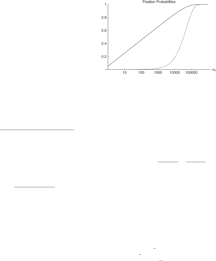
Figure 1.—Fixation probabilities from a single new muta-
RESULTS
tion (dashed line) and from a single segregating allele (solid
line). Note that ␣
b
is measured on a logarithmic scale.
Fixation probability from the standing genetic varia-
tion: The fixation probability of an allele A with selective
advantage s
b
that segregates in a population at frequency
to segregate at a given frequency is proportional to the
x is given by Kimura’s diffusion approximation result:
inverse of the frequency, (x
k
) ⫽ a
⫺
1
N
e
k
⫺
1
, where x
k
⫽ k/2
N
e
and a
N
e
⫽ 兺
2N
e
⫺
1
k
⫽
1
(1/k). The average fixation probability
⌸
x
(␣
b
, h) ⬇
冮
x
0
exp[⫺␣
b
(2hy ⫹ (1 ⫺ 2h)y
2
)]dy
冮
1
0
exp[⫺␣
b
(2hy ⫹ (1 ⫺ 2h)y
2
)]dy
(1)
is then
⌸
seg
⫽ 兺
2N
e
⫺
1
k
⫽
1
⌸
x
k
(x
k
). We derive an exact result
for ⌸
seg
in terms of a hypergeometric function in the
appendix; for 2N
e
Ⰷ 2h␣
b
Ⰷ 1 we obtain the approxima-
tion
(Kimura 1957). In the following, we assume that selec-
tion on the heterozygote is sufficiently strong (formally,
we need 2h␣
b
Ⰷ (1 ⫺ 2h)/2h). We can then ignore the
⌸
seg
(h␣
b
, N
e
) ⬇ 1 ⫺
|ln(2hs
b
)|
ln(2N
e
)
⫽
ln(2h␣
b
)
ln(2N
e
)
. (3)
term proportional to y
2
in Equation 1 and ⌸
x
is approxi-
mately
We can make two interesting observations from this result.
First, as is seen in Figure 1, there is a large increase in
⌸
x
(h␣
b
) ⬇
1 ⫺ exp[⫺2h␣
b
x]
1 ⫺ exp[⫺2h␣
b
]
. (2)
the (average) fixation probability if an allele does not
arise as a single new copy, but already segregates in the
population. This increase is particularly large for small
If A enters the population as a single new copy, x ⫽
adaptations, which points to the second observation: For
1/2N
e
, and if 2N
e
Ⰷ 2h␣
b
Ⰷ 1, we recover Haldane’s
alleles from the standing genetic variation, the fixation
classic result that the fixation probability is twice the
probability depends only weakly (logarithmically) on
heterozygote advantage, ⌸
1/2N
e
⬇ 2hs
b
(Haldane 1927).
the selection coefficient. Indeed, ⌸
seg
, unlike ⌸
x
, does
This relation underlines the importance of genetic drift:
not show a linear dependence on h␣
b
even if h␣
b
is very
It is not sufficient for an advantageous allele to arrive
small. The reason is that, conditioned on later fixation,
in a population, it also needs to escape stochastic loss.
the average frequency of the allele at the time of the
Due to the strong linear dependence of the fixation
environmental change, x
k
, increases with decreasing
probability on the selection coefficient, alleles with a
h␣
b
, such that 2h␣
b
x
k
⬎ 1 for all h␣
b
[a simple calculation
small beneficial effect are less likely to escape such loss.
in the appendix reveals that x
k
⬇ 1/ln(2h␣
b
)]. The usual
The fixation process thus acts like a stochastic sieve that
linear approximation of ⌸
x
is therefore never appro-
favors adaptations with large effects. This was stressed
priate.
in particular by Kimura (1983). According to Equation
Consider, now, an allele A that segregates in the popu-
2, an approximately linear dependence of ⌸
x
on h␣
b
lation at an equilibrium of mutation, (negative) selec-
holds more generally as long as either the initial fre-
tion, and drift when the environment changes at time
quency x or the heterozygote advantage h␣
b
is small,
T. For t ⬎ T, positive selection sets in. We are interested
such that 2h␣
b
x ⬍ 1.
in the net probability P
sgv
that the allele is available
Let us now compare this view of the fixation process
in the population at time T and subsequently goes to
with the alternative scenario of adaptation from the
fixation. In the continuum limit for the allele frequen-
standing genetic variation. In the most simple case, the
cies, P
sgv
is given by the integral
allele A again originates from a single mutation, but
before the environmental change, and already segregates
P
sgv
⫽
冮
1
0
(x)⌸
x
dx, (4)
in the population under neutrality when positive selec-
tion sets in. Standard results (e.g., Ewens 2004) show
that under these conditions the probability for an allele where
⌸
x
is the fixation probability (Equation 2) and

2338 J. Hermisson and P. S. Pennings
(x) is the density function for the frequency of a de- can be obtained by numerical integration of Equation
4, using the allele frequency distributions Equations 5rived allele in mutation-selection-drift balance. Approxi-
mations for (x) can be obtained from standard diffu- and 6. It is instructive to compare the stochastic result,
Equation 8, with the deterministic approximation used bysion theory; all derivations are given in the appendix.
In the neutral case (␣
d
⫽ 0) the distribution of derived Orr and Betancourt (2001). If we set x ⬅ ⌰
u
/2h⬘␣
d
in
Equation 2 (the equilibrium value at mutation-selectionalleles is approximately
balance), the fixation probability from the standing varia-
tion becomes
(x) ⬇ C
0
x
⌰
u
⫺
1
1 ⫺ x
1
⫺⌰
u
1 ⫺ x
. (5)
P
sgv
(h␣
b
, h⬘␣
d
, ⌰
u
) ⬇ 1 ⫺ exp(⫺⌰
u
h␣
b
/h⬘␣
d
). (10)
For a previously deleterious allele and 2h⬘␣
d
Ⰷ (1 ⫺
Equation 8 reduces to Equation 10 if and only if there
2h⬘)/2h⬘, we obtain
is relatively strong past deleterious selection such that
R
␣
Ⰶ 1. In this limit, the initial frequency of the selected
(x) ⬇ C
␣
x
⌰
u
⫺
1
exp(⫺2h⬘␣
d
x)
1 ⫺ exp[2h␣
d
(x ⫺ 1)]
1 ⫺ x
.
allele is sufficiently reduced that the fixation probability
⌸
x
(Equation 2) is approximately linear in x over the
(6)
range of (x), ⌸
x
⬇ 2h␣
b
x. In the integral (4) then only
the average allele frequency x enters, which (almost)
C
0
and C
␣
are normalization constants. (x) includes a
coincides with the deterministic approximation. For
probability Pr
0
that A is not present in the population
R
␣
ⱖ 1, the distribution (x) feels the concavity of ⌸
x
at time T. For ⌰
u
⬍ 1, this probability is approximately
and the true value of P
sgv
drops below the deterministic
estimate. This is captured by Equation 8; see Figure 2.
Pr
0
(h⬘␣
d
, N
e
) ⬇
冢
2N
e
2h⬘␣
d
⫹ 1
冣
⫺⌰
u
For R
␣
ⱕ 1 the fixation probability does not approach
the “deterministic” approximation even if N
e
and thus ␣
d
,
⫽ exp(⫺⌰
u
ln[2N
e
/(2h⬘␣
d
⫹ 1)]). (7)
␣
b
, and ⌰
u
get large. The reason is that it is the variance
For the probability that the population successfully adapts
of 2h␣
b
x that matters, which does not go to zero even if
from the standing variation we derive the simple approxi-
the variance of the allele frequency Var[x] → 0 for large
mation
⌰
u
and ␣
d
.
Equations 8 and 9 confirm a weak dependence of the
P
sgv
(h␣
b
, h⬘␣
d
, ⌰
u
) ⬇ 1 ⫺
冢
1 ⫹
2h␣
b
2h⬘␣
d
⫹ 1
冣
⫺⌰
u
fixation probability on ␣
b
. For fixed ␣
d
, the fixation
probability depends logarithmically on ␣
b
(and on R
␣
)
as long as R
␣
⬎ 1. In the “deterministic limit” R
␣
Ⰶ 1,
⫽ 1 ⫺ exp(⫺⌰
u
ln[1 ⫹ R
␣
]),(8)
this dependence goes back to linear. However, this is true
where R
␣
:⫽ 2h␣
b
/(2h⬘␣
d
⫹ 1) is the relative selective
only if ␣
b
varies independently of ␣
d
. If stronger selected
advantage. R
␣
measures the selective advantage of A in
alleles have larger trade-offs, i.e., ␣
b
and ␣
d
are positively
the new environment relative to the forces that cause
correlated, R
␣
and thus P
sgv
and ⌸
seg
will increase less
allele frequency changes in the ancestral environment,
than linearly with ␣
b
even if R
␣
Ⰶ 1. Using the determinis-
deleterious selection and drift (represented by the 1).
tic aproximation, Orr and Betancourt (2001) pre-
We refer to R
␣
⬍ 1 and R
␣
⬎ 1 as cases of small and
viously found that the dominance coefficient drops out
large relative advantage, respectively. If the allele A is
of P
sgv
if dominance does not change upon the environ-
completely recessive in the old environment (h⬘⫽0),
mental shift, h ⫽ h⬘. The stochastic result Equation 8
similar approximations hold here and below if 2h⬘␣
d
⫹
confirms this finding and extends it beyond the limits
1inR
␣
is formally replaced by
√
␣
d
⫹ 1 (see again the
of validity of the deterministic approximation as long
appendix for details). To relate Equation 8 to Equation
as h␣
b
and h⬘␣
d
are both large.
3, we need to calculate the fixation probability for a
Standing variation vs. new mutations: We want to com-
segregating allele that is derived from a single mutation
pare the fixation probability from the standing variation
prior to the environmental change. This probability is
with the probability that an adaptive substitution occurs
obtained from (8) and (7) by conditioning on segrega-
from new mutation. The probability for a new allele to
tion of the allele in the limit ⌰
u
→ 0. We find
occur in the population that is destined for fixation is
ⵑp
new
⫽ 2N
e
u2hs
b
per generation. Using a Poisson approxi-
⌸
seg
(h␣
b
, h⬘␣
d
, N
e
) ⬇
ln[1 ⫹ R
␣
]
ln[2N
e
/(2h⬘␣
d
⫹ 1)]
. (9)
mation, the probability that such a mutation arrives within
G generations is
For ␣
d
⫽ 0 and h␣
b
Ⰷ 1 this reduces to Equation 3.
P
new
(G) ⫽ 1 ⫺ exp[⫺⌰
u
h␣
b
G], (11)
All further results of our study depend on Equation
8. Computer simulations show that this simple analytical where G is measured in units of 2N
e
. We can now deter-
mine the number of generations G
sgv
that it takes forexpression is quite accurate over a large parameter
range (assuming ⌰
u
⬍ 1 and h␣
b
, h⬘␣
d
Ⰶ 2N
e
; see Figure P
new
(G
sgv
) ⫽ P
sgv
. This value serves as a measure of the
relative adaptive potential of the standing variation. Us-2). Slightly better approximations (which coincide with
95% confidence intervals of all our simulation runs) ing Equation 8 we obtain
2339Soft Sweeps
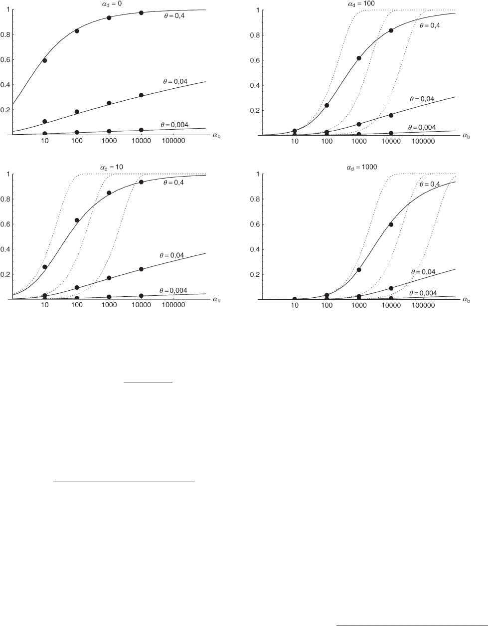
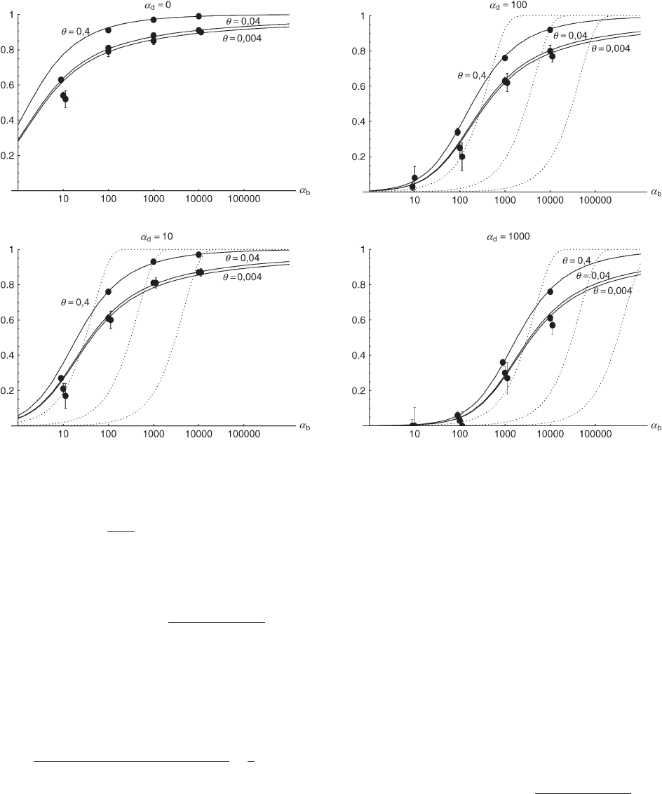
Figure 2.—The probability of fixation from mutation-selection-drift balance, P
sgv
, for a range of mutation and selection
parameters. Solid lines show approximation Equation 8 and dotted lines show the deterministic approximation Equation 10.
Solid circles are simulation results. Ninety-five percent confidence intervals are contained in the circles.
environmental change, or both. Computer simulations
G
sgv
(h␣
b
, h⬘␣
d
) ⬇
ln[1 ⫹ R
␣
]
h␣
b
. (12)
that include new mutations after time T show that hy-
brid fixations that use material from both sources are
This value is independent of ⌰
u
and depends only on
quite frequent for high ⌰
u
, but also that the contribu-
the selection parameters of the allele. One can relate
tion of the standing variation generally dominates in
G
sgv
to the average fixation time t
fix
of an allele with
this case (for ⌰
u
⫽ 0.4 on average 67–97%, depending
selective advantage h␣
b
. In the appendix, we derive t
fix
on ␣
b
and ␣
d
). In the following, we combine hybrid
in units of 2N
e
,
fixations with fixations that use only alleles from the
standing variation and define P
sgv
more broadly as the
t
fix
(h␣
b
) ⬇
2(ln[2h␣
b
] ⫹ 0.577 ⫺ (2h␣
b
)
⫺
1
)
h␣
b
. (13)
probability that an adaptive substitution uses material
from the standing genetic variation. With this definition,
simulation results are closely matched by the theoreticalThe approximation is very accurate for h ⫽ 0.5 and
prediction in Equation 8.
h␣
b
ⲏ 2. For h ⬆ 0.5 it defines a lower bound. We see
We can now ask for the probability that a derived
that G
sgv
⬍ t
fix
for arbitrary R
␣
. This holds even if we
allele A, which is found in the population some time G
account for the fact that the average fixation time from
after T, and either fixed or destined to go to fixation
the standing variation may be shorter (but ⱖ t
fix
/2),
at this time, originated (at least partially) from alleles
since the allele starts at a higher frequency. This result
in the standing genetic variation. Measuring G in units
means that in a time span that an allele from the stand-
of 2N
e
generations, this probability may be expressed
ing variation needs to reach fixation, it is at least as likely
as Pr
sgv
⫽ P
sgv
/(P
sgv
⫹ (1 ⫺ P
sgv
)P
new
). With Equation 8,
that the allele alternatively appears as a new mutation
destined for fixation only after the environmental
Pr
sgv
(␣
b
, ␣
d
, ⌰
u
) ⬇
1 ⫺ exp{⫺⌰
u
ln[1 ⫹ R
␣
]}
1 ⫺ exp{⫺⌰
u
(ln[1 ⫹ R
␣
] ⫹ h␣
b
G)}
.
change.
Next, we consider the case that a derived beneficial
(14)
mutation A is found in a population some time after
the environmental change. There are three possibilities:
In Figure 3, this is shown for G ⫽ 0.05, i.e., for a time
A derives from the standing genetic variation at time
of 0.1N
e
generations after the environmental change.
This time should be sufficiently long for significant adap-T, or from new mutation(s) that occurred after the
2340 J. Hermisson and P. S. Pennings
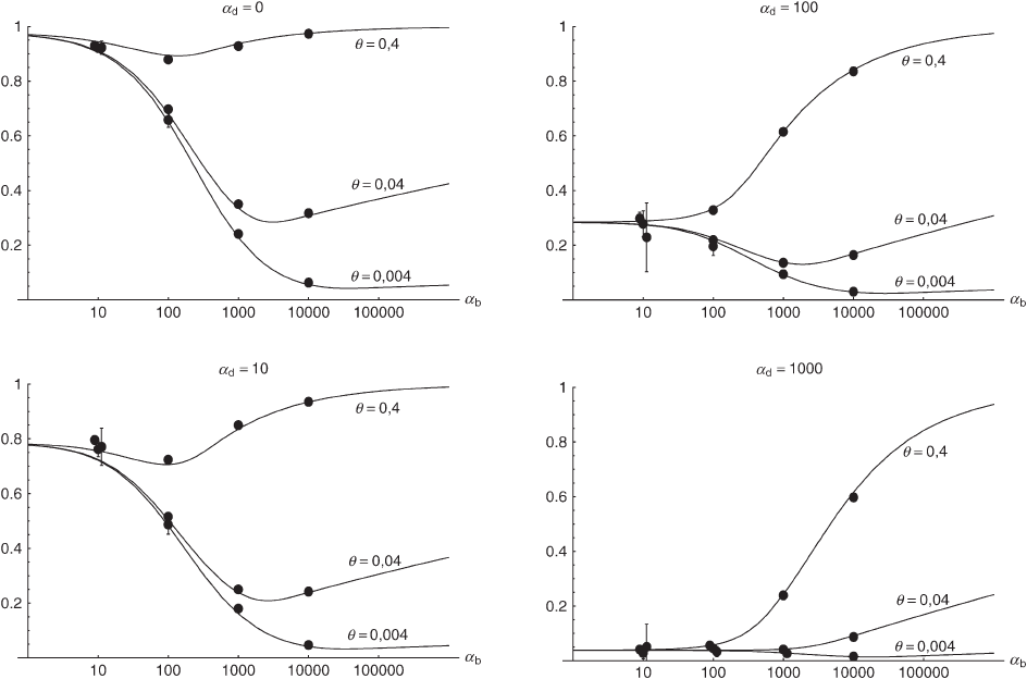
Figure 3.—The probability that an adaptive substitution is from the standing genetic variation (Pr
sgv
). Simulation data with
95% confidence intervals are compared to the analytical approximation Equation 14.
tive change, but still short enough for a selective sweep sufficiently high that there is no need to wait for a new
mutation to occur.to be detected in DNA sequence data (Kim and Stephan
2000; Przeworski 2002). For Drosophila melanogaster, For practical application of this result, remember that
Pr
sgv
does not count only alleles that are fixed at time0.1N
e
generations approximately correspond to the time
since it expanded its range out of Africa into Europe T ⫹ G, but also alleles that are destined to go to fixation.
Consequently, simulations in Figure 3 are continuedafter the last glaciation (i.e., ⵑ10,000–15,000 years ago).
There are two advantages of the standing variation until loss or fixation of the allele even beyond T ⫹ G.
This makes almost no difference as long as the averageover adaptations purely from new mutations. First, the
standing genetic variation may already contain multiple fixation time t
fix
of an allele is much smaller than G.
However, if t
fix
ⱖ G, Equation 14 can no longer be usedcopies of the later-beneficial allele, reducing the proba-
bility of a stochastic loss relative to a single copy. This to predict full substitutions. For G ⫽ 0.1N
e
, t
fix
⬎ G
if h␣
b
ⱗ 275. If we count only substitutions that areadvantage is measured in the relative adaptive potential
G
sgv
above. A second, independent advantage is that completed at time T ⫹ G, P
new
is more strongly reduced
than P
sgv
. For alleles with t
fix
⬇ G, predominance of thealleles from the standing variation are immediately avail-
able and may outcompete new mutations due to this standing genetic variation is larger than that predicted
by Equation 14 (confirmed by simulations, results nothead start. Consequently, we see that substitutions from
the standing variation dominate in two parameter re- shown). For alleles with t
fix
Ⰷ G practically all substitu-
tions that are completed at time T ⫹ G contain materialgions. First, they dominate for small h␣
b
as long as selec-
tion before the environmental change was also weak be- from the standing variation; however, there are then
only very few fixations at all.cause P
sgv
⬎ P
new
in this range. (P
sgv
⬎ P
new
for h␣
b
⬍ ln[1 ⫹
R
␣
]/G ; for small h␣
b
this needs h⬘␣
d
⬍ 1/G, i.e., ␣
d
⬍ 40 Population bottlenecks: So far, we have assumed that
the effective population size before, during, and afterfor h⬘⫽0.5 and G ⫽ 0.1N
e
.) The second parameter region
is if h␣
b
and the mutation rate ⌰
u
are both high. In this the environmental change is constant. For many evolu-
tionary scenarios, however, it may be more realistic tocase, the crucial advantage of the alleles from the standing
genetic variation is their immediate availability: The proba- assume that the shift of the environmental conditions
is accompanied by a population bottleneck. Examplesbility for fixation from the standing variation is already

2341Soft Sweeps
include colonization events and human domestication, tion to N
T
. Here, is the intrinsic growth rate (for t in
but also the (temporary) reduction of the carrying ca-
units of 2N
0
), and K the carrying capacity. There are
pacity of a maladapted population in a changed environ-
two things to note. First, the effect of recovery on the
ment.
fixation probability is significant only if it is sufficiently
Suppose that a population of ancestral size N
0
goes
fast on a scale set by the selection strength. For logistic
through a bottleneck directly after the environmental
recovery, this is the case if ⲏh␣
b
. Second, the increase
change and recovers afterward until it reaches its car-
of the fixation probability due to recovery is much more
rying capacity in the new environment. We want to know
important for P
sgv
than for P
new
. The reason is that only
how these demographic events change the probability
alleles that are already present during the bottleneck
Pr
sgv
that a substitution is derived from the standing
will be affected. While this is the case for all alleles
genetic variation. We expect two factors to play a role.
from the standing variation that survive population size
On the one hand, a deep and long-lasting bottleneck
reduction, only relatively few new mutations will occur
may significantly reduce the standing variation and the
in the small bottleneck population (at least if recovery
potential of the population to adapt from it. On the
is sufficiently fast to matter). More formally, one can
other hand, a slow or incomplete recovery reduces the
show that the increase in the fixation probability due
opportunity for new mutations to arrive in the popula-
to recovery can be neglected in P
new
if G Ⰷ 1. This
tion and thus the probability of adaptation from new
leaves only a very restricted parameter space of h␣
b
ⱗ
mutations.
ⱗ1/G, where an increase in fixation probability plays
It is therefore instructive to distinguish two elements
a role for P
new
(confirmed by simulations, not shown).
of a bottleneck, population size reduction and subse-
In the following, we concentrate on fast recovery on
quent recovery, and discuss their effects separately. The
a scale of G, i.e., Ⰷ1/G (results for slow recovery
simplest case is a pure reduction of N
0
by a factor B ⬎
are intermediate between fast and no recovery). As a
1 at time T, with no recovery. For matters of comparison,
measure for the opportunity for new beneficial muta-
we continue to use the ancestral population size N
0
in
tions to arrive in the population, let N
av
be the average
the definitions of ⌰
u
, ␣
b
, ␣
d
, and G. In our formulas for
population size from time T to time T ⫹ G, where the
the fixation probabilities from new or standing variation
substitutions are censused. We then define a bottleneck
(Equations 8, 11, and 14) population size reduction is
parameter for new mutations B
new
:⫽ N
0
/N
av
and rescale
then simply included by a rescaling of the selection
␣
b
to ␣
b
/B
new
in P
new
(Equation 11). For fixations from
parameter ␣
b
to ␣
b
/B. (For adaptations from the stand-
the standing genetic variation, we define the bottleneck
ing genetic variation note that a sampling step to gener-
strength as B
sgv
(h␣
b
) ⫽ N
0
/N
fix
(h␣
b
) and rescale the rela-
ate a bottleneck does not change the frequency distribu-
tive selection strength R
␣
→ R
␣
/B
sgv
in Equations 8 and
tion of the later-beneficial allele, leaving ␣
b
in Equation
14. Here, N
fix
is an average “fixation effective population
2 the only parameter subject to change. For adaptation
size” that is felt by a beneficial allele on its way to fixation
from new mutations the rescaling argument follows if
or loss. Since the sojourn time of a strongly selected
we express the probability for a new mutation destined
allele is shorter than that of a weakly selected allele, N
fix
for fixation per generation as p
new
⫽ (2N
e
/B)u2hs
b
⫽
and B
sgv
depend on the selection coefficient of the allele.
2uh␣
b
/B.) Consequently, the graphs in Figure 3 are
For logistic growth, Equation 19 in Otto and Whitlock
simply shifted to the right. A pure reduction of the
(1997) leads to
population size at time T thus reduces the relative advan-
tage of the standing genetic variation for strongly se-
B
sgv
(h␣
b
) ⫽
N
0
N
T
·
h␣
b
⫹N
T
/K
h␣
b
⫹
. (15)
lected alleles with a large mutation rate, but enhances
its advantage for weakly selected alleles. Note that the
Figure 4 shows the percentage of fixations from the
adaptive potential G
sgv
increases by a factor of B relative
standing variation for a bottleneck with N
T
⫽ N
0
/100 and
to t
fix
and can now be much larger than the fixation
logistic recovery with ⵑ5% initial growth per generation
time.
and carrying capacity K ⫽ 2546. More precisely, we
Relative to a simple reduction in population size, re-
choose ⫽0.05092 · 2N
0
⫽ 2546 for the growth rate
covery increases the adaptation probability from the
per 2N
0
⫽ 50,000 generations, such that the average size
standing variation, P
sgv
, and from new mutations, P
new
,
after the environmental change until 0.1N
0
generations
in different ways. First, recovery increases P
new
(but not
(i.e., G ⫽ 0.05) is N
av
⫽ N
0
/10 ⫽ 2500.
P
sgv
) simply due to the fact that the opportunity for new
From Equation 15 and Figure 4, we can distinguish
mutations increases with increasing population size. Sec-
three parameter regions for the effect of a bottleneck.
ond, the fixation probability of beneficial alleles is in-
First, for h␣
b
⬎, the fixation probability of individual
creased due to population growth. For further progress,
alleles is not substantially increased by population
we use results on the fixation probability in populations
growth as compared to the case without recovery. How-
of changing size by Otto and Whitlock (1997). We
ever, population growth increases the opportunity for
assume that the population experiences logistic growth
according to dN/dt ⫽(1 ⫺ N/K)N after an initial reduc- new mutations and thus B
new
⬍ B
sgv
. For large ⌰
u
, there
2342 J. Hermisson and P. S. Pennings
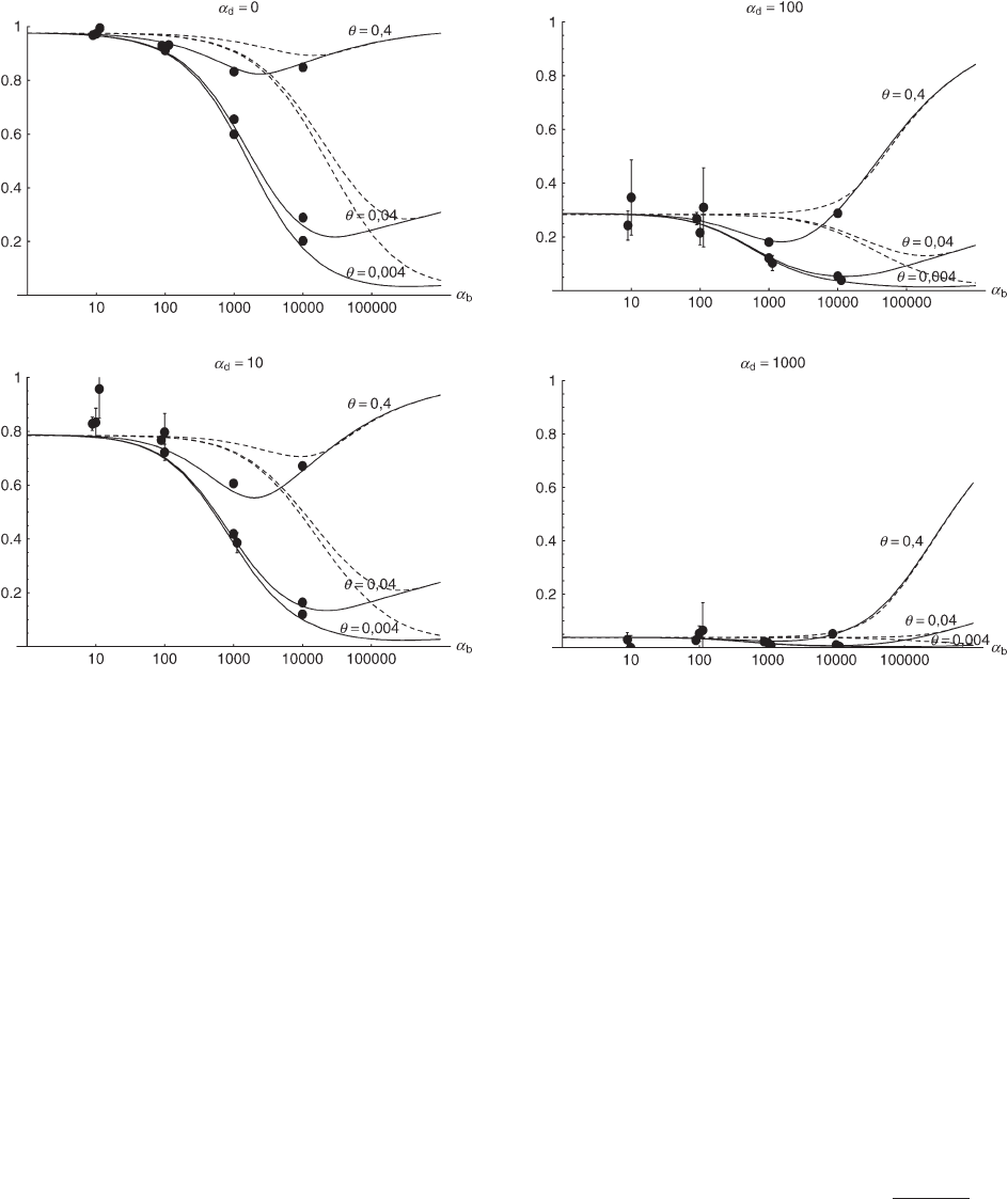
Figure 4.—The probability that an adaptive substitution stems from the standing genetic variation Pr
sgv
in a population with
a bottleneck at the time of the environmental change. Dashed lines show a simple reduction in population size by a factor 100
without recovery. Simulation circles and solid lines are for the opposite case of strong logistic recovery (for parameters see main
text). The lines follow from the simple analytical approximation Equation 14 with the bottleneck correction R
␣
→ R
␣
/B
sgv
and
␣
b
→ ␣
b
/B
new
in the term proportional to G. Direct numerical integration of Equations 5 and 6 with the same bottleneck correction
produces a slightly better fit.
is nevertheless almost no change in Pr
sgv
relative to no copies are involved in the substitution, one may expect
recovery. The reason is that fixation is then almost cer-
differences in the footprint of the adaptation on linked
tain, with P
new
⬇ 1 and thus Pr
sgv
⬇ P
sgv
(see the definition
neutral variation. To derive the probability that n copies
of Pr
sgv
above Equation 14). Second, for very small selec-
of the allele A that segregate in the population at time
tion coefficients, h␣
b
⬍N
T
/K, all alleles feel the new
T contribute to its fixation, we follow Orr and Betan-
carrying capacity K as their fixation effective population
court (2001) and assume that individual copies enjoy
size. If Ⰷ1/G, the bottleneck then acts like a single
an independent probability to escape stochastic loss.
change in the population size from N
0
to K. Finally, for
We may then apply a Poisson approximation. If the
intermediate selection coefficients, P
new
generally pro-
frequency of A at the time of the environmental change
fits more from the recovery than P
sgv
, leading to a reduc-
is x, the probability that k ⫽ n copies survive and contrib-
tion in Pr
sgv
if compared to no recovery.
ute to fixation is approximately
Compared with the results of the previous section,
we can summarize the effect of a bottleneck as follows.
Pr(k ⫽ n; x) ⫽ exp[⫺2h␣
b
x]
(2h␣
b
x)
n
n!
. (16)
There is a tendency to further increase the predomi-
nance of the standing variation for weakly selected al-
This approximation is consistent with Equation 3 if 2h␣
b
Ⰷ
leles and to decrease its advantage for high h␣
b
and ⌰
u
.
1. The probability that more than one copy contributes
However, unless the bottleneck is very strong, there is
to the substitution (i.e., the probability for a “soft sweep”)
no qualitative change in the overall pattern.
is then Pr(k ⬎ 1; x) ⫽ 1 ⫺ (1 ⫹ 2h␣
b
x)exp[⫺2h␣
b
x].
Footprints of soft sweeps: Since adaptations from the
Averaging over the allele frequency distribution at time
standing genetic variation start out with a higher copy
T, (x), and conditioning on the case that fixation did
number of the selected allele, more than one of these
occur, we obtain the probability for a soft sweep for
copies may escape stochastic loss and eventually contrib-
ute to fixation. Depending on whether one or multiple adaptations from the standing genetic variation,
2343Soft Sweeps
Figure 5.—The probability that multiple copies from the standing genetic variation contribute to a substitution, P
mult
. Solid
lines correspond to Equation 18 and dotted lines to the deterministic approximation Equation 19.
frequency and weak positive selection, the Poisson ap-
P
mult
⬇ 1 ⫺
2h␣
b
P
sgv
冮
1
0
xexp[⫺2h␣
b
x](x)dx. (17)
proximation is no longer valid.
To estimate the impact of a soft sweep on linked
Using the approximation Equations 5 and 6 for the
neutral variation we are also interested in the number
allele distribution and Equation 8 for P
sgv
, this gives
of independent copies that contribute to the fixation of
the allele, i.e., copies that are not identical by descent.
P
mult
(R
␣
, ⌰
u
) ⬇ 1 ⫺
⌰
u
R
␣
/(1 ⫹ R
␣
)
(1 ⫹ R
␣
)
⌰
u
⫺ 1
, (18)
Concentrating on copies that segregate in the popula-
tion at the time T of the environmental change, we
can again use a Poisson approximation, P
˜
r(k ⫽ n) ⫽
which reduces to P
mult
⬇ 1 ⫺ R
␣
/((1 ⫹ R
␣
)ln[1 ⫹ R
␣
])
exp(⫺)
n
/n!. With this conjecture, 1 ⫺ exp(⫺) is the
in the limit ⌰
u
→ 0. This limit is essentially reached for
fixation probability from the standing genetic variation.
⌰
u
ⱗ 0.004. We can again compare the stochastic result
Equating with P
sgv
as given in Equation 8, we obtain ⫽
with the deterministic approximation that is obtained
⌰
u
ln[1 ⫹ R
␣
]. The probability of fixation of multiple
from Equation 17 assuming x ⬅ ⌰
u
/2h⬘␣
d
,
independent copies, conditioned on the cases where
fixation occurs then is
P
mult
⬇
exp[⌰
u
h␣
b
/h⬘␣
d
] ⫺ 1 ⫺⌰
u
h␣
b
/h⬘␣
d
exp[⌰
u
h␣
b
/h⬘␣
d
] ⫺ 1
⬇
1
2
⌰
u
h␣
b
/h⬘␣
d
.
(19)
P
ind
(R
␣
, ⌰
u
) ⬇ 1 ⫺
⌰
u
ln[1 ⫹ R
␣
]
(1 ⫹ R
␣
)
⌰
u
⫺ 1
. (20)
Both approximations, Equations 18 and 19, are com-
pared to simulation data in Figure 5. The deterministic Alternatively, we obtain Equation 20 from Equation 18
using the relation 1 ⫺ P
mult
(⌰
u
) ⫽ (1 ⫺ P
ind
(⌰
u
))(1 ⫺approximation reproduces the stochastic result only for
very large mutation rates, ⌰
u
Ⰷ 1, outside the parameter P
mult
(⌰
u
⫽ 0)). This equation expresses the probability
for fixation of a single copy (“no multiple fixation givenspace in the figure. For low mutation rates, where Equa-
tion 19 predicts a zero limit for ⌰
u
→ 0 it severely under- fixation”) as the probability of fixation from a single
origin times the probability of fixation of a single copyestimates P
mult
. The stochastic approximation produces
a reasonable fit unless h⬘␣
d
and h␣
b
are both small. In given that all successful copies are from a single origin
(a single origin is enforced in P
mult
by ⌰
u
→ 0). Thisthis parameter range with relatively high initial allele
2344 J. Hermisson and P. S. Pennings
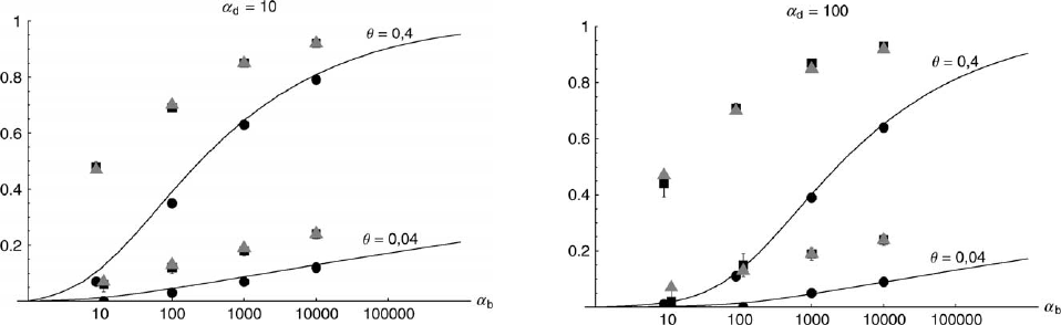
Figure 6.—The probability that multiple copies with independent origin contribute to a substitution, P
ind
. Lines correspond
to Equation 20; symbols represent simulation data. Circles represent fixations from the standing genetic variation without new
mutational input after time T; squares include new mutations. Triangles represent fixations from recurrent new mutations only.
alternative derivation shows that Equations 18 and 20 becomes almost independent of ␣
d
. Even more impor-
tantly, we see that the fixation of multiple independentfollow from the same assumption: independent fixation
probability for different copies. To the order of our copies is not particular to adaptations from the standing
genetic variation. It occurs with basically the same proba-approximation, P
mult
and P
ind
depend on selection only
through the relative selective advantage R
␣
⫽ 2hs
b
/ bility if the selected allele enters the population after
the environmental change as a recurrent new mutation(2h⬘s
d
⫹ 1/(2N
e
)). This parameter combines two effects.
The denominator of R
␣
takes into account that multiple (see Figure 6, triangles).
For recurrent new mutations, the simulation datafixations are less likely if the initial frequency of the
allele at time T is low. This frequency decreases with show that the total fixation rate of multiple independent
copies, r
ind
⫽⫺ln[1 ⫺ P
ind
], increases logarithmicallydeleterious selection h⬘s
d
and drift, represented by the
1/2N
e
term. Second, the numerator of R
␣
accounts for with ␣
b
and linearly with ⌰
u
. For a heuristic understand-
ing of this dependence, assume h ⫽ 0.5 and let x(t)bethe fixation probability of the allele: The probability
that the allele is maintained during the adaptive phase the frequency of a first copy of the selected allele on
its way to fixation in the absence of further mutation.increases with hs
b
. For h␣
d
Ⰷ 1, the result depends only
on the ratio of the selection coefficients as also predicted For small u, the probability for a second copy of the
beneficial mutation to arise while a first copy spreads toby the deterministic approximation (Orr and Betan-
court 2001). If the environmental change is followed fixation is then p
2
⫽ 2N
e
u兰
∞
0
(1 ⫺ x(t))dt ⫽ 2N
e
u(2N
e
t
fix
/2). Here, t
fix
is the average fixation time in 2N
e
gener-by a bottleneck, Equations 18 and 20 can be used with
R
␣
→ R
␣
/B
sgv
with the bottleneck factor introduced ations and we have used that the first copy spends on
average equal times in frequency classes x and (1 ⫺ x ).above. In contrast to P
mult
, the fixation probability of
multiple independent copies depends strongly on the By far the largest contribution to p
2
comes from the
early phase of the sweep where the frequency x of themutation rate ⌰
u
and vanishes for ⌰
u
→ 0. In Figure
6, Equation 20 is compared with simulation data. The first copy is very low. The probability of the second copy
to survive until fixation of the allele depends on x, butapproximation produces a good fit for ␣
d
ⱖ 10 where
the Poisson approximation is valid. to leading order only the survival probability for x → 0
matters, which is approximately s
b
. With t
fix
from Equa-By construction, both approximations (18) and (20)
account only for the fixation of copies of the allele that tion A17 we then obtain r
ind
⫽⌰
u
ln(␣
b
) ⫹ ᏻ(␣
0
b
). A
more detailed account will be given elsewhere.were already in the population at time T. It is, however,
also possible that a successful copy first arises for t ⬎ TP
ind
is the probability that descendants of multiple
independent copies of the selected allele segregate inas a new mutation during the adaptive phase. Since the
origin of these new copies is necessarily independent, the population at the time when this allele reaches fixa-
tion. Consequently, the number of copies in our simula-this effect contributes to P
ind
. The size of this contribution
depends on the population-level mutation rate ⌰
u,t
⬎
T
di- tion runs was counted at the time of fixation (same for
P
mult
). In practical applications, however, one is oftenrectly after the environmental change. ⌰
u,t
⬎
T
can be
smaller than the original ⌰
u
that appears in Equations 18 interested in the probability of observing descendants
from independent origins a fixed time G after an envi-and 20 if there is a bottleneck at T. For ⌰
u,t
⬎
T
⫽⌰
u
our simulation results show that the contribution of new ronmental change. This probability will decrease with
G, since copies get lost by drift until, eventually (in themutations to P
ind
is substantial (Figure 6, squares). One
consequence of mutational input after T is that P
ind
absence of back mutation), all copies derive from a
2345Soft Sweeps
single mutation as their common ancestor. The drift than the average neutral coalescent time. We want to
analyze whether and how the contribution of multiplephase from the time of fixation to the time of observa-
tion G depends on the selection coefficient and will be copies to an adaptive substitution affects the signature
of selection on linked neutral variation. For this, it islonger for strongly selected alleles with short fixation
times. In principle, this could affect the dependence of helpful to distinguish two aspects of a selective footprint,
its width in base pairs along the sequence and its maxi-the probability of observing multiple fixed copies in a
population on h␣
b
. To test this, we ran additional simula- mum depth in terms of the extent of variation lost in
a region close to the locus of selection.tions to measure the probability for the survival of multiple
(independent) copies G ⫽ 0.1N
e
generations after the For a hard sweep, the coalescent at the selected site
itself does not extend beyond time T. Ancestral variationenvironmental change (results not shown). For alleles
with fixation time t
fix
⬍ 0.1N
e
, we did not detect any that has existed prior to T can be maintained only if
there is recombination between the selected site anddifference from the data displayed in Figures 5 and 6,
meaning that fixation of a single copy in the neutral the site studied. In a core region around the selected
site, where no recombination has happened, all ances-drift phase after initial fixation of multiple copies is
rare. This is not surprising, considering that the average tral variation is lost. Recombination therefore modu-
lates the width of the sweep region, but in general doesfixation time under neutral drift exceeds 0.1N
e
genera-
tions even if the frequency of the major copy is initially not affect its maximum depth. Since only recombination
in the selective phase matters, and since the adaptiveat 99%.
Another question is whether multiple copies of the phase is much shorter for a strongly selected allele, the
width of a selective footprint decreases with larger ␣
b
.selected allele are likely to be found in a small experi-
mental sample, even if they exist in the population. We For a soft sweep, the coalescent at the selected site
itself extends into the ancestral environment. As com-tested this by arbitrarily drawing 12 chromosomes in
each case of a soft sweep. Multiple copies in the sample pared with a hard sweep, a soft sweep therefore has a
reduced maximum depth. Our results show that softwere found in 70–80% of all cases (for ⌰
u
⫽ 0.4). Sum-
marizing our results for the fixation probabilities of sweeps with shallower footprints are more likely for large
␣
b
. This does not contradict that selective footprints getmultiple copies and of multiple independent copies, we
can distinguish three parameter regions: weaker and eventually vanish as ␣
b
→ 0, for two reasons.
First, even if it is more likely for lower ␣
b
that all ancestral
Low mutation rate, relatively strong past selection: If
variation is eliminated close to the selection center, the
the mutation rate is low (⌰
u
Ⰶ 0.1) fixation of multiple
width of the window where this holds true gets smaller
independent copies of the selected allele is unlikely.
at the same time. If this width drops below the average
If multiple copies fix, they are most likely identical
distance of polymorphic sites, the footprint of selection
by descent. If past deleterious selection is strong, how-
becomes undetectable. Second, if we observe the sweep
ever, also the fixation of multiple homologous copies
region G generations after positive selection begins, we
is rare. For ⌰
u
⫽ 0, Equation 18 indicates that ⬍5%
can compare only selective footprints of alleles that have
and ⬍30% of fixations originate from multiple copies
reached fixation by this time. If we want to study very
for R
␣
ⱕ 0.1 and R
␣
⫽ 1, respectively (Figure 5).
weakly selected alleles, G needs to be so large that any
Low mutation rate, relatively weak past selection: With
footprint of selection will be washed out by new muta-
increasing relative advantage R
␣
the fixation of multi-
tions that arise after time T.
ple homologous copies increases. For ⌰
u
→ 0, fixation
The impact of a soft sweep on the molecular signature
of multiple copies occurs in ⬎50% of the cases (P
mult
⬎
depends on whether the surviving copies are indepen-
0.5) if R
␣
ⲏ 4 (Figure 5).
dent by descent or not. Copies from different origins
High mutation rate: For mutation rates ⌰
u
ⲏ 0.1 fixa-
are related by a neutral coalescent and represent inde-
tions from independent origins are much more fre-
pendent ancestral haplotypes. If these haplotypes are
quent and become more likely than the fixation of
sampled close to the locus of selection, this should mark
single copies. This holds true for whether the origin
a clearly visible difference from the classic pattern of a
of the selected allele is from the standing variation
hard sweep. A detailed quantitative analysis with esti-
or from recurrent new mutations. The fixation proba-
mates of the impact on summary statistics for nucleotide
bility for multiple independent copies increases loga-
variability exceeds the aims of this study and will be
rithmically with h␣
b
. For ⌰
u
⫽ 0.4, 50–90% of substitu-
given elsewhere.
tions involve multiple independent copies (Figure 6).
If multiple surviving copies are identical by descent,
the expected change in the molecular footprint relativeImagine that we observe a DNA region where an adap-
tive substitution has happened following an environ- to a hard sweep depends on the strength of deleterious
selection that the allele has experienced prior to themental change at time T. Suppose that we observe this
region G generations after the environmental change, environmental change. We expect a shallower footprint
(and larger deviation from the hard sweep) for weakerand 2 Ⰷ G Ⰷ t
fix
, such that the advantageous allele has
reached fixation, but G (in units of 2N
e
) is much shorter deleterious selection. The reason is that it is more likely
2346 J. Hermisson and P. S. Pennings
for a weakly deleterious allele to segregate in a popula- hard sweeps from a new mutation in this case. For a
rough estimate of when this difference should be detect-tion for a long time; i.e., the average time to the most
recent common ancestor in the core region of the sweep able, we compare the total fixation times of the allele
A in the case of a soft sweep, t
fix ,soft
(s
d
, s
b
), with theis larger for smaller ␣
d
. Indeed, this intuition can be
made more precise. average duration of a sweep from a new mutation t
fix
(s
b
)
(cf. Equation 13). For an optimal (that is, minimal) timeA remarkable property of the Markov process that
underlies the Wright-Fisher model is that, conditional of observation G ⬇ t
fix
(s
b
), we expect a clear difference
in the selective signatures if the increase in coalescenceon an allele A having reached some frequency x in a
population, this process is independent of the sign of time is of the same order of magnitude as the original
coalescence time. Estimating the relative change in co-the selection coefficient of A (cf. Ewens 2004, Chaps.
4.6 and 5.4; for simplicity, we assume ⌰
u
⫽ 0 and h ⫽ alescence time by the change in fixation time, this
means t
⌬
⫽ t
fix,soft
(s
d
, s
b
) ⫺ t
fix
(s
b
) ⲏ t
fix
(s
b
). We deriveh⬘⫽0.5). This has interesting consequences for adapta-
tions from mutation-selection-drift balance. Assume that t
⌬
from the frequency distribution of the allele at the
time T conditional on multiple fixation and results froman allele A with selective disadvantage s
d
that is derived
from a single mutation segregates in the population at diffusion theory on the expected age of an allele given
its frequency; details are given in the appendix. Thefrequency x at the time T of the environmental change.
Then the mean age of this allele and, more generally, results (not shown) predict visible changes in the sweep
pattern for a minimum of R
␣
between 20 and 100.the average time that it spent in each frequency class
in the past are the same as if it had a selective advantage
of the same absolute size prior to T. Assume that A
DISCUSSION
spreads to fixation under positive selection with selec-
tion coefficient s
b
after the environmental change and The adaptive process is the genetic response of a
population to external challenges. In nature, these chal-compare this with a sweep of an (imaginary) allele A⬘
with the same frequency x at time T, but selective advan- lenges may be due to changes in climate or food re-
sources or arise with the advent of a new predator ortage s
b
throughout. For s
d
⫽ s
b
, the total fixation time
of the alleles and their sojourn times in every frequency parasite. They either affect the original habitat of the
population or are a consequence of the colonization ofclass are the same; for s
d
⬍ s
b
(resp. s
d
⬎ s
b
) they are
longer (shorter) for A. a new niche or of human artificial selection. In this article,
we are interested in the adaptive response of a previouslyThe above argument shows that the footprint of a
sweep from the standing genetic variation is identical well-adapted population to a sudden and permanent
change. We concentrate on a single locus with twoto a “usual” sweep pattern if the selection coefficient
changes its sign, but not its absolute value upon the (classes of) alleles, one, a, ancestral, and the other, A,
derived. Allele A is either neutral or deleterious underenvironmental change. If we observe the sweep region
at time G, the only difference from a sweep that has the original conditions, but selectively advantageous
after the change in the selection regime at some timeoriginated from a new mutation after time T is the
somewhat older age of the sweep from the standing T. We compare two scenarios: either A already segre-
gates in the population at time T and fixes from thevariation. For s
d
⬆ s
b
, the change in the selection regime
leads to differences in the expected footprint of alleles standing genetic variation or the population adapts
from a new copy of the allele that enters the populationA and A⬘. Clearly, this difference is due to the cases
where the coalescent of A (and A⬘) extends into the old only after the environmental shift.
Our results rely on two main assumptions. First, andenvironment, i.e., where the sweep is “soft.” For s
d
⬎ s
b
,
the expected coalescence in the ancestral environment most importantly, we assume that adaptation of the tar-
get allele does not interfere with positive or negativeis faster for A than for A⬘, leading to a stronger footprint
of selection. However, since soft sweeps are very rare selection on other alleles, through either linkage or
epistasis. This assumption is usually made in populationfor s
d
⬎ s
b
, this will hardly lead to a detectable difference
in the average footprint. genetic studies of selective sweeps. It is satisfied if the
rate of selective substitutions is low and the time toLet us now concentrate on the case s
b
⬎ s
d
,orR
␣
⬎
1, where soft sweeps are frequent. In this case, the coales- fixation for each individual substitution is short, but is
less plausible for weakly selected alleles with long aver-cence in the ancestral environment is slower and the
selective signature for A is reduced in depth and width age fixation times. In general, interference reduces fix-
ation probabilities, with a stronger influence on weakrelative to A⬘ (due to the increased opportunity for
mutation and recombination until the allele is fully coa- substitutions (Barton 1995), although this does not
translate into a large effect on the reduction of heterozy-lesced). If the frequency x of the allele at time T is large,
the sweep pattern of A will look more like a sweep of gosity due to a selective sweep (Kim and Stephan 2003).
In their study of fixation probabilities of alleles froman advantageous allele with a selection coefficient of
size s
d
⬍ s
b
. We therefore also expect to find a larger the standing variation, Orr and Betancourt (2001)
did not find a large effect of interference. This, however,difference between the footprints of soft sweeps and
2347Soft Sweeps
may be a consequence of the neglect of new mutations than the subsequent beneficial effect of the allele, mean-
ing that the relative selective advantage R
␣
⫽ 2h␣
b
/and the restriction to a low initial frequency of the
selected allele in their simulations. These assumptions (2h⬘␣
d
⫹ 1) ⬍ 1. Our study extends their analysis to
arbitrary values of R
␣
. The simple analytical approxima-make it unlikely that two or more beneficial alleles es-
cape early stochastic loss and compete on their way to tion for the probability of a substitution from the stand-
ing variation (Equation 10 above, resp. Equation 3 infixation. We therefore emphasize that our results are
conditional on noninterference. Second, we assume that Orr and Betancourt 2001), which uses the determin-
istic value for the initial frequency of A in mutation-the variation at the locus under consideration is main-
tained in mutation-selection-drift balance prior to the selection balance, is no longer valid in the general case.
Nevertheless, there is an equally simple expression,environmental change. If selected alleles are main-
tained as a balanced polymorphism or are not in equilib- Equation 8, which serves as an approximation for the
entire parameter range.rium at all, this may clearly affect our conclusions.
Our results pertain to three main issues: the depen- Our results corroborate and extend the findings of
Orr and Betancourt (2001). To the order of ourdence of fixation probabilities on selection coefficients
if alleles are taken from the standing genetic variation, approximation, the fixation probability from the stand-
ing genetic variation depends on selection only throughthe relative importance of the standing variation and
new mutations as the origin of adaptive substitutions, R
␣
. If selection is strong in both environments, and h⬘⫽
h, it is independent of dominance. More generally, ifand the expected impact of a selective sweep from the
standing genetic variation on linked nucleotide varia- beneficial and deleterious effects of alleles in different
environments were strictly proportional, the distributiontion. We discuss them in turn.
Fixation probability from the standing variation: In of the effects of adaptations from the standing variation
would coincide with the distribution of the effects of newa famous argument that helped to found the micro-
mutationist view of the adaptive process, Fisher (1930) beneficial mutations, as implicitly assumed in Fisher’s
(1930) argument. The reason is the same as in the caseshowed that mutations with a small effect are much
more likely to be beneficial than mutations with a large of dominance: Advantages in the fixation probability
due to a larger ␣
b
are compensated by disadvantageseffect. Kimura (1983), however, pointed out a flaw in
this argument: Even if a large majority of new beneficial due to a smaller initial frequency with higher ␣
d
.
Remarkably, we find that the stochastic sieve is sub-mutations has a small effect, as Fisher argues, this may
be offset by a much smaller fixation probability of weakly stantially weakened even if alleles with a larger selective
advantage do not have a larger disadvantage to compen-selected alleles. An allele with (constant) heterozygote
advantage hs
b
that enters the population as a single new sate for it. If alleles are originally neutral or under rela-
tively weak deleterious selection, such that R
␣
⬎ 1, therecopy will escape stochastic loss and spread to fixation
with probability 2hs
b
. One can think of stochastic loss is only a very weak logarithmic dependence of the fixa-
tion probability on all parameters for selection or domi-as a sieve where small-effect alleles pass through the
holes—and vanish from the population—much more nance. The reason is the high initial frequency of the
successful alleles in this case, which may be much higheroften than alleles with a large selective advantage. A
variant of this picture is known as Haldane’s sieve and than the average frequency of all segregating alleles. At
these high frequencies, the fixation probability is onlypertains to different levels of dominance: Substitutions
are likely to be dominant since dominant alleles enjoy weakly dependent on the selection coefficient of the
allele. There is, however, a sieve acting against alleleshigher fixation rates.
This latter scenario is the subject of Orr and Betan- under disproportionately large past selection, R
␣
⬍ 1.
If the selected physiological function (with fixed h␣
b
)court (2001), who study Haldane’s sieve if selected
alleles are taken from the standing genetic variation. is met by several alleles with different h⬘␣
d
, alleles with
a relatively mild deleterious effect in the past, h⬘␣
d
⬍They conclude that the sieve is not active in this case.
If the selected allele is deleterious under the original h␣
b
, will be preferred. Note that this should confer
a certain level of resilience to the population if theconditions (with heterozygote disadvantage h⬘s
d
), and
if the level of dominance is maintained upon the envi- environmental conditions change back.
Empirical estimates of R
␣
, the relative selectionronmental shift, h ⫽ h⬘, the net fixation probability is
approximately independent of dominance. It is easy to strength, are difficult to obtain and generally not avail-
able. There is no a priori reason to assume that s
b
isunderstand why: The advantage of a higher fixation rate
with larger h is compensated by the lower frequency either larger or smaller than s
d
(s
b
⬍ s
d
was assumed by
Orr and Betancourt 2001). To see this, note that theof the initially deleterious allele in mutation-selection
balance. Orr and Betancourt (2001) focus on a lim- roles of the alleles A and a and the selection coefficients
s
b
and s
d
are exchanged if the environment changes backited parameter range, where the selected allele is defi-
nitely deleterious under the original conditions and to the old conditions at some later time. This argument
does not pertain to the average selection coefficient ofthus starts at a low frequency. In their calculations, they
also assume that the original deleterious effect is larger any deleterious allele (which is plausibly larger than
2348 J. Hermisson and P. S. Pennings
the average beneficial effect), but only to the selection cially pronounced if the environmental shift is fol-
lowed by a bottleneck with incomplete recovery. Thecoefficients of deleterious alleles that are beneficial in
the new environment. Several factors can cause an up- percentage of substitutions that use alleles from the
standing variation is then almost independent of theward or downward bias of R
␣
. R
␣
is downward biased
if there is a bottleneck at the time of the environmental mutation rate since ⌰
u
affects the fixation probabilities
from standing and new variation in the same way.change. In this case, the effective population size that
enters ␣
b
is reduced relative to the original N
e
that enters 2. The standing variation is also important for alleles
with a large relative selective advantage (R
␣
Ⰷ 1) if␣
d
. An upward bias in R
␣
could result from a change
in dominance following the environmental shift. To see the mutation rate ⌰
u
is also high. In this case, fixation
probabilities are high under both scenarios, new mu-this, assume that alleles a and A serve different func-
tions that are only (or mostly) used in the old and new tations and standing genetic variation. Since the
standing variation other then new mutations is imme-environments, respectively. The physiological theory of
dominance claims that the common observation of domi- diately available, it will usually contribute a major
share to the substitution. Note that R
␣
Ⰷ 1 is plausiblenant wild-type alleles is a natural consequence of multien-
zyme biochemistry (e.g., Kacser and Burns 1981; Orr in particular for “important” adaptations with large
effect, such as insecticide-resistance alleles. Whether1991; Keightley 1996). If this holds true, it is natural
to expect that there is at least partial dominance of the such an adaptation likely originated from the stand-
ing genetic variation then depends mainly on ⌰
u
.respective advantageous (wild-type) allele, hence of a
(A) in the old (new) environment, and thus h ⬎ h⬘.
Selective footprints of soft sweeps: For a classical
Finally, if R
␣
is measured among successful substitutions
sweep from a single new mutation, which we call a hard
from the standing genetic variation, a further upward
sweep, ancestral variation can be preserved only if there
bias results from the stochastic sieve against alleles with
is recombination between the polymorphic locus and
large h⬘␣
d
.
the selection target during the selective phase. In a
Relative importance of adaptations from the standing
“core” region around the selection center all ancestral
variation and from new mutations: To estimate the im-
variation is erased. In contrast, with a soft sweep, multiple
portance of the standing genetic variation as a reservoir
copies of the selected allele contribute to the substitu-
for adaptations, we compare a polymorphic population,
tion. Depending on the history of these copies, part of
in mutation-selection-drift balance, with a monomor-
the ancestral variation may then be maintained and
phic one. We can measure the additional adaptive po-
appear as haplotype structure in the population. There
tential of the polymorphic population in the number of
are two types of soft sweeps. For the first type, multiple
generations G
sgv
that a monomorphic population must
copies that contribute to the substitution derive from
wait for sufficiently many new mutations to arrive to
independent mutations. For the second type, multiple
match the fixation probability from the standing varia-
copies that existed at the time of the environmental
tion. G
sgv
can be very large for mutations with small
change contribute to the substitutions, but these copies
effect (of the order 1/hs
b
generations). However, for a
are identical by descent.
population of constant size it is always smaller than the
Soft sweeps of the first type (independent origins)
average fixation time of the allele. This means that there
are frequent if the mutation rate on the population
is no clear separation of adaptive phases: By the time
level is sufficiently high (⌰
u
ⲏ 0.1); see Figure 6. Their
most alleles from the standing genetic variation with
probability relative to a sweep from a single origin also
a given selective advantage h␣
b
have reached fixation,
increases with the selection strength h␣
b
, i.e., altogether
substitutions from new mutations (with the same h␣
b
)
for alleles with high adaptive rates. Suprisingly, soft
will also be found. Only if the environmental change is
sweeps of this type are not exclusive to adaptations from
followed by a strong reduction in population size is the
the standing genetic variation, but occur with the same
reservoir of the standing variation exploited well before
probability for adaptations that originate only from new
new mutations start to play a role.
mutations, which have entered the population after the
We have also determined the probability that the
environmental change. Even if material from the stand-
standing variation contributes to an adaptive substitu-
ing variation is used, most soft sweeps with copies from
tion that is observed some time G after an environmen-
independent origins also involve new mutations. Since
tal change. Clearly, this probability generally declines
surviving copies represent independent ancestral haplo-
with G. For fixed G there are two distinct parameter
types, we expect characteristic differences in the selec-
regions where the standing variation is most important.
tive footprint relative to the classic pattern of a hard
sweep, where only a single ancestral haplotype survives1. Adaptations from the standing variation are favored
for alleles with small effect that are under relatively in the core region close to the selection site. A discussion
of the effect of soft sweeps on the summary statistics forweak past selection, R
␣
ⱖ 1. This is a direct conse-
quence of the stochastic sieve that eliminates weak nucleotide variation will be given elsewhere.
Soft sweeps of the second type (copies with a commonalleles in a new mutation scenario. The effect is espe-
2349Soft Sweeps
origin prior to the environmental change) can occur Third, while hard sweeps from single mutations pro-
duce the strongest footprint for strongly selected allelesonly for adaptations from the standing genetic variation.
They are frequent even for a very low mutation rate with short fixation times, the possibility of fixation of
multiple alleles leads to an opposite trend: Soft sweeps⌰
u
→ 0 if the allele has a high relative selective advantage
R
␣
ⲏ 4; see Figure 5. The sweep pattern depends on with weaker footprints are more frequent for high ␣
b
.
Since the increase is only logarithmic, this trend is notthe strength of deleterious selection that the allele has
experienced in the old environment. For R
␣
⬎ 1, we very strong. Nevertheless, it could be visible for nucleo-
tides that are tightly linked to the selected allele in regionsexpect a weaker footprint with a narrower sweep region
than predicted for a hard sweep with the same selective of low recombination or in sufficiently small windows
around the selection target. A genome-wide study ofadvantage h␣
b
. We predict, however, that differences in
the sweep patterns are visible only for a minimum R
␣
the small-scale reduction of heterozygosity in narrow
windows of 200 bp around replacement or silent fixa-of 20–100. For ␣
d
⫽ 0, where the probability of multiple
fixations and the resulting effect on the sweep pattern tions has recently been performed for D. simulans by
Kern et al. (2002). We note that their counterintuitiveare strongest, this has been studied in a recent publica-
tion by Innan and Kim (2004). Using computer simula- finding of a sweep signature for preferred codon substi-
tutions, but not for replacement substitutions, matchestions, these authors indeed find much weaker selective
footprints if the alleles are taken from the standing our prediction of a stronger sweep signal for weakly
selected alleles close to the selection center. However,genetic variation. Since their minimum value of R
␣
is
1000, their results fit our predictions. a quantitative analysis of soft sweeps that also accounts
for other factors like population substructure is neededWe can summarize our results on soft sweeps in three
observations. First, evidence of a soft sweep does not before any conclusions can be drawn.
result in an easy criterion to distinguish adaptive substi-
We thank Sylvain Mousset and Wolfgang Stephan for fruitful discus-
tutions from the standing variation and recurrent new
sions and John Parsch for helpful comments on the manuscript. The
careful comments by Sally Otto and an anonymous reviewer led to
mutations. For a large parameter space we will not be
many clarifying changes. We also thank Pieter van Beek for help with
able to detect any difference between these adaptive
the computer simulations. This work was supported by an Emmy
scenarios. This confirms the conclusion of Orr and
Noether grant from the Deutsche Forschungsgemeinschaft to J.H.
Betancourt (2001), although partly for different rea-
sons. For high ⌰
u
ⲏ 0.1, soft sweeps are frequent in
both cases; for low ⌰
u
and R
␣
ⱗ 20 they either are rare
LITERATURE CITED
in both cases or do not lead to significant differences
Barton, N. H., 1995 Linkage and the limits to natural selection.
in the selective footprints. For a range of “interesting”
Genetics 140: 821–841.
substitutions, namely alleles with a large effect but a low
Barton, N. H., 1998 The effect of hitch-hiking on neutral genealo-
gies. Genet. Res. 72: 123–133.mutation rate, however, the linked nucleotide pattern
Catania, F., M. O. Kauer, P. J. Daborn, J. L. Yen, R. H. Ffrench-
could be informative.
Constant et al., 2004 World-wide survey of an Accord insertion
Second, soft sweeps are frequent in a limited but rele-
and its association with DDT resistance in Drosophila melanogaster.
Mol. Ecol. 13: 2491–2504.vant parameter space. We expect soft sweeps with charac-
Ewens, W. J., 2004 Mathematical Population Genetics, Ed. 2. Springer,
teristic patterns on the selective footprints for high ⌰
u
,
Berlin.
i.e., either if the population size is large or if the allelic
Falconer, D. S., and T. F. C. Mackay, 1996 Introduction to Quantita-
tive Genetics. Addison Wesley Longman, Harlow, Essex, UK.mutation rate is high, such as at mutational hotspots
Fisher, R. A., 1930 The Genetical Theory of Natural Selection. Oxford
or if the adaptation corresponds to a loss-of-function
University Press, Oxford.
mutation of the gene. We also expect soft sweeps for
Haldane, J. B. S., 1927 A mathematical theory of natural and artifi-
cial selection. Part V: selection and mutation. Proc. Camb. Philos.large adaptations with h␣
b
Ⰷ h⬘␣
d
(thus R
␣
Ⰷ 1) from
Soc. 23: 838–844.
the standing variation, even if the mutation rate is small.
Hansen, T. F., C. Pelabon, W. S. Armbruster and M. L. Carlson,
The effect of a soft sweep in this last case is a reduction
2003 Evolvability and genetic constraint in Dalechampia blos-
soms: components of variance and measures of evolvability. J.in the width of the sweep region relative to a hard sweep.
Evol. Biol. 16: 754–765.
A possible candidate for a soft sweep of this type is the
Houle, D., 1992 Comparing evolvability and variability of quantita-
evolution of DDT resistance in non-African populations
tive traits. Genetics 130: 195–204.
Innan, H., and Y. Kim, 2004 Pattern of polymorphism after strongof D. melanogaster. In recent studies of nucleotide and
artificial selection in a domestication event. Proc. Natl. Acad. Sci.
microsatellite variability in the region around an Accord
USA 101: 10667–10672.
insertion that is associated with DDT resistance, Schlenke
Kacser, H., and J. A. Burns, 1981 The molecular basis of domi-
nance. Genetics 97: 6639–6666.
and Begun (2004) and Catania et al. (2004) found evi-
Kaplan, N. L., R. R. Hudson and C. H. Langley, 1989 The “hitch-
dence for a selective sweep. The width of the sweep region,
hiking effect” revisited. Genetics 123: 887–899.
however, was much narrower in D. melanogaster than ex-
Keightley, P. D., 1996 A metabolic basis for dominance and recessi-
vity. Genetics 143: 621–625.pected under putatively very strong selection (Catania et
Kern, A. D., C. D. Jones and D. J. Begun, 2002 Genomic effects
al. 2004) and, as observed, for the “same” adaptation (with
of nucleotide substitutions in Drosophila simulans. Genetics 162:
a Doc insertion) in D. simulans (Schlenke and Begun
1753–1761.
Kim, Y., and W. Stephan, 2000 Joint effects of genetic hitchhiking2004).

2350 J. Hermisson and P. S. Pennings
and background selection on neutral variation. Genetics 155: Maynard Smith, J., and J. Haigh, 1974 The hitch-hiking effect of
a favourable gene. Genet. Res. 23: 23–35.1415–1427.
Kim, Y., and W. Stephan, 2002 Detecting a local signature of genetic Orr, H. A., 1991 A test of Fisher’s theory of dominance. Proc. Natl.
Acad. Sci. USA 88: 11413–11415.hitchhiking along a recombining chromosome. Genetics 160:
765–777. Orr, H. A., and A. J. Betancourt, 2001 Haldane’s sieve and adapta-
tion from the standing genetic variation. Genetics 157: 875–884.Kim, Y., and W. Stephan, 2003 Selective sweeps in the presence of
interference among partially linked loci. Genetics 164: 389–398. Otto, S., and M. C. Whitlock, 1997 The probability of fixation in
Kimura, M., 1957 Some problems of stochastic processes in genetics.
populations of changing size. Genetics 146: 723–733.
Ann. Math. Stat. 28: 882–901.
Przeworski, M., 2002 The signature of positive selection at ran-
Kimura, M., 1983 The Neutral Theory of Molecular Evolution. Cambridge
domly chosen loci. Genetics 160: 1179–1189.
University Press, Cambridge, UK.
Schlenke, T. B., and D. J. Begun, 2004 Strong selective sweep associ-
Kimura, M., and T. Ohta, 1969 The average number of generations
ated with transposon insertion in Drosophila simulans. Proc. Natl.
until fixation of a mutant gene in a finite population. Genetics
Acad. Sci. USA 101: 1626–1631.
61: 763–771.
Steppan, S. J., P. C. Phillips and D. Houle, 2002 Comparative
Lande, R., and S. J. Arnold, 1983 The measurement of selection
quantitative genetics: evolution of the G matrix. TREE 17: 320–
on correlated characters. Evolution 37: 1210–1226.
327.
Lynch, M., and J. B. Walsh, 1998 Genetics and Analysis of Quantitative
Traits. Sinauer, Sunderland, MA. Communicating editor: M. Nordborg
APPENDIX
Fixation probability for a mutation segregating at neutrality: We calculate the average fixation probability of an
allele that is derived from a single mutation and segregates in the population under neutrality at the time T of the
environmental change. The probability that there are exactly k copies at time T is distributed as (k) ⫽ a
N
k
⫺
1
,
where a
N
⫽ 兺
2N
e
⫺
1
k
⫽
1
(1/k). Assuming a selection coefficient s
b
for t ⬎ T and no dominance (h ⫽ 0.5), the average
fixation probability is given by
⌸
seg
(N
e
, s
b
) ⫽
1
a
N
兺
2N
e
⫺
1
k
⫽
1
1 ⫺ exp(⫺ks
b
)
k(1 ⫺ exp(⫺2N
e
s
b
))
⫽
1
1 ⫺ exp(⫺2N
e
s)
冢
1 ⫺
1
a
N
兺
2N
e
⫺
1
k
⫽
1
exp(⫺ks
b
)
k
冣
. (A1)
We derive the sum in (A1) as
兺
2N
e
⫺
1
k
⫽
1
e
⫺
ks
b
k
⫽
冮
∞
s
b
ds
˜
b
兺
2N
e
⫺
1
k
⫽
1
e
⫺
ks
b
⫽
冮
∞
s
b
ds
˜
b
冤
e
⫺
s
˜
b
⫺ e
⫺
2N
e
s
˜
b
1 ⫺ e
⫺
s
˜
b
冥
⫽
冮
∞
s
b
ds
˜
b
冤
1
e
s
˜
b
⫺ 1
冥
⫹
冮
⫺
∞
⫺
s
b
ds
˜
b
冤
e
2N
e
s
˜
b
1 ⫺ e
⫺
s
˜
b
冥
⫽⫺ln(1 ⫺ e
⫺
s
b
) ⫹
2
F
1
(1, 2N
e
,2N
e
⫹ 1, e
⫺
s
b
)
2N
e
e
2N
e
s
b
, (A2)
where
2
F
1
denotes the hypergeometric function. For N
e
s
b
Ⰷ 1, this second term can be neglected and we obtain
⌸
seg
(N
e
, s
b
) ⬇ 1 ⫹
1
a
N
ln(1 ⫺ e
⫺
s
b
). (A3)
In the limit of small s
b
and large N
e
this reduces to
⌸
seg
(N
e
, s
b
) ⬇ 1 ⫹
ln(s
b
)
ln(2N
e
) ⫹␥
, (A4)
where ␥⫽0.577...isEuler’s constant. For weak recessivity, this result holds if we replace s
b
by 2hs
b
.
Fixation probability for allele in mutation-selection-drift balance: To calculate the frequency distribution of a
derived allele, we start out with the Kolmogorov forward equation that describes the Wright-Fisher model in the
diffusion limit (Ewens 2004),
f(x, t)
t
⫽⫺
x
(a(x)f(x, t)) ⫹
1
2
2
x
2
(b(x)f(x, t)), (A5)
where
a(x) ⫽
1
2
(⫺␣
d
x(1 ⫺ x)(2x ⫹ 2h⬘(1 ⫺ 2x)) ⫺⌰
v
x ⫹⌰
u
(1 ⫺ x)) and b(x) ⫽ x(1 ⫺ x) (A6)
are the drift and diffusion terms. Forward mutations are measured by ⌰
u
; back mutations are measured by ⌰
v
. Since
the diffusion process is ergodic, the probability that the frequency of an allele falls into a certain interval [x
1
, x
2
]
is proportional to the average time T that an allele that starts out as a single copy spends in this frequency range

2351Soft Sweeps
before it is either lost or fixed. The frequency distribution therefore directly follows from the well-known transient
behavior of the process, e.g., Ewens (2004, Chap. 4). From Equations 4.23 and 4.16 in Ewens (2004), we obtain
(x) ⫽ C
exp[⫺␣
d
(2h⬘x ⫹ (1 ⫺ 2h⬘)x
2
)]
x
1
⫺⌰
u
(1 ⫺ x)
1
⫺⌰
v
冮
1
x
exp[␣
d
(2h⬘y ⫹ (1 ⫺ 2h⬘)y
2
)]
y
⌰
u
(1 ⫺ y)
⌰
v
dy, (A7)
where C is a normalization constant. Note that this expression deviates from Wright’s stationary distribution of an
allele in mutation-selection-drift balance since we condition on the case that A is derived.
Simple approximate relations for Equation A7 are readily obtained in various limiting cases. First, direct numerical
integration shows that back mutations can safely be ignored even in the neutral case ␣
d
⫽ 0 because most alleles
segregate at low frequencies (this is a consequence of conditioning on derived alleles). In the neutral case, this
approximation directly leads to Equation 5. If there is deleterious selection, we need to distinguish cases of weak
and strong recessivity of the allele A. We concentrate mostly on the case where deleterious selection on the
heterozygote is sufficiently strong, 2h⬘␣
d
Ⰷ (1 ⫺ 2h⬘)/2h⬘ (i.e., weak recessivity). Under these conditions, we can
ignore the quadratic terms in the exponentials and express (x) in terms of incomplete Gamma functions,
(x) ⫽ C⬘ exp(⫺2h⬘␣
d
x)x
⌰
u
⫺
1
(⫺2h⬘␣)
⌰
u
⫺
1
(⌫(1 ⫺⌰
u
, ⫺2h⬘␣
d
x) ⫺⌫(1 ⫺⌰
u
, ⫺2h⬘␣
d
))
1 ⫺ x
, (A8)
with normalization constant C⬘. For definitely deleterious A (2h⬘␣
d
ⱖ 10 is sufficient), the integrand in Equation
A7 is concentrated near y ⫽ 1. We can then expand y
⌰
u
in the denominator to leading order around y ⫽ 1(i.e.,
y
⌰
u
⬇ 1) and obtain (x) in terms of simple functions, which leads to Equation 6.
To obtain an analytical expression for the probability of fixation P
sgv
or multiple fixation P
mult
, we need to
approximate (x) further. If the allele A is neutral prior to the environmental change, and ⌰
u
Ⰶ 1, (x) in Equation
5isⵑ(x) ⬇ ⌰
u
x
⌰
u
⫺
1
. Using this in Equation 4,
P
sgv
(⌰
u
, h␣
b
) ⬇ ⌰
u
冮
1
0
[x
⌰
u
⫺
1
(1 ⫺ exp[⫺2h␣
b
x])]dx ⬇ 1 ⫺
⌫(⌰
u
⫹ 1)
(2h␣
b
⫹ 1)
⌰
u
⬇ 1 ⫺ (2h␣
b
⫹ 1)
⫺⌰
u
, (A9)
where we extend the integral over exp(⫺2h␣
b
x)to∞ after increasing 2h␣
b
by 1 to avoid a singularity near ␣
b
⫽ 0.
We also use ⌫(⌰
u
⫹ 1) ⬇ 1 for 0 ⱕ⌰
u
ⱕ 1.
For the deleterious case (2h⬘␣
d
Ⰷ 1), note that the allele frequency distribution is significantly larger than zero only
for x ⱕ 1/2h⬘␣
d
. Expanding around x ⫽ 0 we can approximate (x) in Equation 6 as (x) ⬇ C ″x
⌰
u
⫺
1
exp(⫺2h⬘␣
d
x)
and obtain
P
sgv
(⌰
u
, h⬘␣
d
, h␣
b
) ⬇ 1 ⫺
冮
1
0
x
⌰
u
⫺
1
exp[(2h⬘␣
d
⫹ 2h␣
b
)x]
dx
冒
冮
1
0
x
⌰
u
⫺
1
exp[2h⬘␣
d
x]
dx ⬇ 1 ⫺
冢
1 ⫹ 2h␣
b
⫹ 2h⬘␣
d
1 ⫹ 2h⬘␣
d
冣
⫺⌰
u
, (A10)
which gives Equation 8. In Equation A10, we have again extended integral limits after adding 1 to 2h⬘␣
d
, respectively
2h␣
b
⫹ 2h⬘␣
d
. We now see that the approximation for 2h⬘␣
d
Ⰷ 1 reproduces the approximation for ␣
d
⫽ 0 in the limit
␣
d
→ 0. We can therefore use it in the entire parameter range. For ⌰
u
⬍ 1, the probability that the allele A is not
contained in the standing variation at time T can be approximated by the integral over (x) from 0 to 1/2N
e
(confirmed
by simulations; see also Ewens 2004, Chap. 5.7). With the above approximations for (x) this results in Equation 7.
Finally, also P
mult
is obtained by an analogous calculation.
If the allele A is completely recessive prior to the environmental change, h⬘⫽0, we again obtain an expression in
incomplete Gamma functions for (x) similar to Equation A8. For large ␣
d
, this reduces to
(x) ⬇
␣
⌰
u
/2
d
exp[⫺␣
d
x
2
]
⌫(⌰
u
/2)x
1
⫺⌰
u
. (A11)
Using this expression in Equation 4, we see that the term exp[⫺␣
d
x
2
] can be ignored as long as 2h␣
b
⬎
√
␣
d
since the
integral is cut off by exp[⫺2h␣
b
x]. For 2h␣
b
⬍
√
␣
d
, both selection coefficients are important. We can obtain a simple,
yet compared to simulation data (not shown) reasonable, analytic approximation that captures this crossover behavior
by formally replacing 2h⬘␣
d
⫹ 1by
√
␣
d
⫹ 1 in Equations 8, 7, and 18 if h⬘⫽0.
The average frequency of the allele A at time T conditioned on later fixation, x
fix
, is calculated from the distribution
Pr(x|fix) ⫽ C(x)⌸
x
(h␣
b
). With the above approximations for (x), we obtain
x
fix
⬇
⌰
u
2h⬘␣
d
⫹ 1
1 ⫺ (1 ⫹ R
␣
)
⫺
(
⌰
u
⫹
1)
1 ⫺ (1 ⫹ R
␣
)
⫺⌰
u
. (A12)
For ⌰
u
→ 0, this gives

2352 J. Hermisson and P. S. Pennings
x
fix
⬇
R
␣
(2h⬘␣
d
⫹ 1)(1 ⫹ R
␣
)ln[1 ⫹ R
␣
]
. (A13)
Finally, if also ␣
d
⫽ 0 and 2h␣
b
Ⰷ 1,
x
fix
⬇
2h␣
b
(2h␣
b
⫹ 1)ln(2h␣
b
⫹ 1)
⬇
1
ln(2h␣
b
)
. (A14)
For the calculation of the average increase in the age of a selected allele for a soft sweep with a weak trade-off, we
use the frequency distribution of the allele at time T conditioned on multiple fixation, Pr(x|mfix) ⬇ C(x)(⌸
x
(h␣
b
))
2
.
[We use the Poisson approximation Equation 16 and 2h␣
b
x ⬇ 1 ⫺ exp(⫺2h␣
b
x) for small x, where (x) is large.] We
consider only the case ⌰
u
→ 0 and h ⫽ h⬘⫽0.5. For a given allele frequency x at time T, we determine the average
age t
a
(␣
d
, x) of the allele using Equation 5.113 in Ewens (2004) (see also Kimura and Ohta 1969),
t
a
(␣
d
, x) ⫽
2
␣
d
(e
␣
d
⫺ 1)
冮
x
0
(e
␣
d
y
⫺ 1)(e
␣
d
(1
⫺
y)
⫺ 1)
y(1 ⫺ y)
dy ⫹
2(1 ⫺ e
⫺␣
d
x
)
␣
d
(1 ⫺ e
⫺␣
d
)(e
␣
d
(1
⫺
x)
) ⫺ 1
冮
1
0
e
⫺␣
d
(1
⫺
y )
(e
␣
d
(1
⫺
y)
⫺ 1)
2
y(1 ⫺ y)
dy. (A15)
The increase in the age of the allele due to the change of the selection regime then is obtained by numerical
integration as t
⌬
⫽ 兰(t
a
(␣
d
, x) ⫺ t
a
(␣
b
, x))Pr(x|mfix)dx. Choosing x ⫽ 1, Equation A15 allows for a simple approxima-
tion for the fixation time of a new allele with selective advantage ␣
b
. We derive
t
fix
(␣
b
) ⫽
2
␣
b
(exp[␣
b
] ⫺ 1)
冮
1
0
(exp[␣
b
y] ⫺ 1)(exp[␣
b
(1 ⫺ y)] ⫺ 1)
y(1 ⫺ y)
dy
⫽
4
␣
b
(exp[␣
b
] ⫺ 1)
冮
1
0
(exp[␣
b
y] ⫺ 1)(exp[␣
b
(1 ⫺ y)] ⫺ 1)
y
dy. (A16)
For ␣
b
ⱖ 3, this may be approximated as
t
fix
(␣
b
) ⬇
4
␣
b
冮
1
0
1 ⫺ exp[⫺␣
b
y] ⫺ exp[␣
b
(y ⫺ 1)] ⫹ exp[⫺␣
b
]
y
dy ⬇
4
␣
b
(ln[␣
b
] ⫹␥⫺␣
⫺
1
b
), (A17)
where ␥ ⬇ 0.577 is Euler’s Gamma. The error term is of order ␣
⫺
3
b
. To the best of our knowledge, this simple result
has not yet been used in the literature. Simulation results of our own (not included) and in Kimura and Ohta
(1969) show that the estimate is very accurate. For h ⬆ 0.5, we can replace ␣
b
by 2h␣
b
in Equation A17. The
approximation then holds as a lower bound for t
fix
, since the fixation time increases if h deviates from 0.5 in either
direction.
