U.S. DEPARTMENT OF COMMERCE
National Oceanic and Atmospheric Administration
National Marine Fisheries Service
NOAA Technical Memorandum NMFS-NWFSC-42
Viable Salmonid Populations
and the Recovery
of Evolutionarily Significant Units
June 2000
NOAA Technical Memorandum
NMFS Series
The Northwest Fisheries Science Center of the National
Marine Fisheries Service, NOAA, uses the NOAA
Technical Memorandum NMFS series to issue informal
scientific and technical publications when complete
formal review and editorial processing are not
appropriate or feasible due to time constraints.
Documents published in this series may be referenced in
the scientific and technical literature.
The NMFS-NWFSC Technical Memorandum series of
the Northwest Fisheries Science Center continues the
NMFS-F/NWC series established in 1970 by the North-
west & Alaska Fisheries Science Center, which has since
been split into the Northwest Fisheries Science Center
and the Alaska Fisheries Science Center. The
NMFS-AFSC Technical Memorandum series is now
being used by the Alaska Fisheries Science Center.
Reference throughout this document to trade
names does not imply endorsement by the National
Marine Fisheries Service, NOAA.
This document should be cited as follows:
McElhany, P., M.H. Ruckelshaus, M.J. Ford, T.C.
Wainwright, and E.P. Bjorkstedt. 2000. Viable
salmonid populations and the recovery of
evolutionarily significant units. U.S. Dept. Commer.,
NOAA Tech. Memo. NMFS-NWFSC-42,156 p.
NOAA Technical Memorandum NMFS-NWFSC-42
Viable Salmonid Populations
and the Recovery
of Evolutionarily Significant Units
Paul McElhany, Mary H. Rucklelshaus, Michael J. Ford, Thomas C.
Wainwright, and Eric P. Bjorkstedt*
Northwest Fisheries Science Center
Conservation Biology Division
2725 Montlake Boulevard East
Seattle, Washington 98112-2097
*Southwest Fisheries Science Center
Santa Cruz/Tiburon Laboratory, Salmon Analysis Branch
3150 Paradise Drive
Tiburon, California 94920-1211
June 2000
U.S. DEPARTMENT OF COMMERCE
William M. Daley, Secretary
National Oceanic and Atmospheric Administration
D. James Baker, Administrator
National Marine Fisheries Service
Penelope D. Dalton, Assistant Administrator for Fisheries

ii
Most NOAA Technical Memorandums NMFS-NWFSC are
available on-line at the Northwest Fisheries Science Center
web site (http://www.nwfsc.noaa.gov)
Copies are also available from:
National Technical Information Service
5285 Port Royal Road
Springfield, VA 22161
phone orders (1-800-553-6487)
e-mail orders (orders @ntis.fedworld.gov)
iii
Table of Contents
List of Figures vii
List of Tables ix
List of Boxes xi
EXECUTIVE SUMMARY xiii
DEFINING A VIABLE SALMONID POPULATION 1
Introduction......................................................................................................................... 1
Purpose and Scope .................................................................................................. 1
Definitions............................................................................................................... 2
Short-term Risk Evaluations ............................................................................................... 4
Population concepts............................................................................................................. 4
General definitions .................................................................................................. 4
Definition of a population that NMFS will use in applying the VSP concept........ 5
Distinction between Population Definition and Tools for Estimation.................... 6
Structure below and above population level........................................................... 6
Borderline situations in defining populations ......................................................... 7
Relationship of the Population Definition to the ESU Definition........................... 7
Population Definition and Artificial Propagation................................................... 9
PARAMETERS FOR EVALUATING POPULATIONS 11
Introduction to Parameters................................................................................................ 11
Population parameters........................................................................................... 11
Guidelines for each population parameter............................................................ 11
Population Size.................................................................................................................. 12
Population Growth Rate and Related Parameters............................................................. 13
Spatial Structure................................................................................................................ 18
Diversity............................................................................................................................ 19
Integrating the parameters and determining population status.......................................... 23
ESU VIABILITY 25
Introduction....................................................................................................................... 25
Number and Distribution of Populations in a Recovered ESU......................................... 25
Populations not meeting VSP guidelines.......................................................................... 27
IMPLEMENTING THE VSP GUIDELINES 29
Introduction....................................................................................................................... 29
Practical Application......................................................................................................... 29
Uncertainty, Precaution, and Adaptive Management........................................................ 29
Interim Application........................................................................................................... 30
Examples........................................................................................................................... 31
APPENDIX 33
Applying VSP in the Regulatory Arena............................................................................ 33
Listing Criteria ...................................................................................................... 33
Recovery................................................................................................................ 34
Jeopardy................................................................................................................ 35
Relationship of VSP to Other Concepts............................................................................ 35
Relationship to Minimum Viable Population Concepts........................................ 35
Relationship to Quantitative Population Viability Analysis................................. 36
Relationship to Properly Functioning Conditions................................................. 36
iv
Relationship to the Sustainable Fisheries Act (SFA) and Maximum Sustainable
Yield (MSY).......................................................................................................... 37
Relationship to Other Conservation Assessment Approaches.............................. 38
Identifying Populations..................................................................................................... 38
Introduction to identifying populations................................................................. 38
Types of Information Used in Identifying Populations......................................... 38
Evidence for independent populations ...................................................... 39
Indicators of population structure ............................................................. 41
Geographic and habitat indicators................................................. 44
Demographic indicators ................................................................ 46
Genetic indicators.......................................................................... 49
Identifying populations—combining the evidence................................... 51
Existing Approaches to Identifying Salmon Populations or Groups .................... 51
Population Size.................................................................................................................. 53
Introduction....................................................................................................................... 53
Density effects........................................................................................... 54
Environmental variation............................................................................ 57
Genetic processes...................................................................................... 58
Demographic stochasticity........................................................................ 61
Ecological feedback .................................................................................. 62
Assessment Methods............................................................................................. 63
Guidelines.............................................................................................................. 64
Population Growth Rate and Related Parameters............................................................. 64
Introduction........................................................................................................... 64
Why population growth rate is important ................................................. 67
Why intrinsic productivity and density dependence are important........... 68
Why stage-specific productivity is important ........................................... 69
Why ancillary data relevant to productivity are important ....................... 73
Estimating Population Growth Rate and Related Parameters............................... 77
Estimating population growth rate and changes in other parameters........ 78
Estimating population growth rate and detecting trends........................... 79
Detecting other pattern in time series: autocorrelation, interventions, and
epochs........................................................................................................ 80
Estimating intrinsic productivity and detecting density dependence........ 81
Critical assumptions .................................................................................. 81
Bias and methods for correcting it ............................................................ 82
Analyses that incorporate stage-specific dynamics................................... 83
Analyses of populations that include naturally spawning hatchery fish... 84
Spatial Structure................................................................................................................ 90
Introduction........................................................................................................... 90
General Spatial Patterns........................................................................................ 91
Why Spatial Structure is Important....................................................................... 91
Metapopulation theory.............................................................................. 91
Source-sink dynamics ............................................................................... 94
Importance of patch spacing...................................................................... 96
Fragmented habitats .................................................................................. 97
v
Assessing Spatial Structure................................................................................... 97
Straying..................................................................................................... 97
Habitat dynamics....................................................................................... 98
VSP Guidelines: Spatial Structure ...................................................................... 101
Diversity.......................................................................................................................... 101
Types of Diversity............................................................................................... 101
Why Diversity is Important................................................................................. 102
Factors that Affect Diversity............................................................................... 102
Risks to Diversity................................................................................................ 105
Selection.................................................................................................. 108
Straying and gene flow............................................................................ 114
VSP Guidelines: Diversity.................................................................................. 122
Viable ESUs.................................................................................................................... 124
Catastrophes........................................................................................................ 124
Long-term Demographic and Evolutionary Processes........................................ 125
ESU Viability Guidelines.................................................................................... 126
LITERATURE CITED 127
vi
vii
List of Figures
Figure 1. This figure illustrates why subpopulations, populations, and ESUs are likely to have a
biological basis................................................................................................................................ 8
Figure 2. Theoretical types of spatially structured populations.................................................... 20
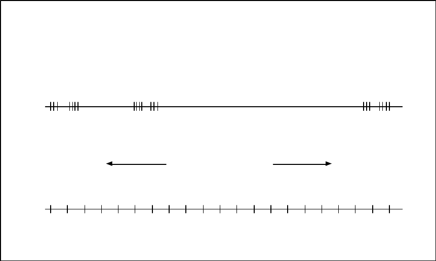
Figure A1a. Distributions of dispersal distances of eelgrass (Zostera marina) based on pollen
and seed dispersal.......................................................................................................................... 42
Figure A1b. Frequency distributions of pollen, seed and combined pollen and seed dispersal
estimated by identifying and mapping seedlings and parents....................................................... 43
Figure A2. The figure shows why demographic independence is theoretically a useful factor in
designating populations................................................................................................................. 47
Figure A3. Typical shape of parent-offspring (or stock-recruit) curves for populations with no
density-dependence (“Linear”), compensation only, and compensation plus depensation. ......... 55
Figure A4. Estimates of spawner:spawner production for Oregon coastal coho salmon
(Oncorhynchus kisutch) in three GCGs. ....................................................................................... 70
Figure A5. Estimates of pre-harvest-recruit:spawner production for Oregon coastal coho salmon
(Oncorhynchus kisutch) in three GCGs. ....................................................................................... 71
Figure A6. Estimates of exploitation rates for three GCGs (North-Mid Coast, Umpqua, Mid-
South Coast) of Oregon coastal coho salmon (Oncorhynchus kisutch) and estimated total
exploitation rate for coho salmon in the Oregon Production Index Area based on analyses of
coded wire tag recoveries.............................................................................................................. 72
Figure A7. Changes in parameters of a composite Beverton-Holt model for smolt yield as a
function of prespawner abundance for four putative life-history variants of spring chinook
salmon (Oncorhynchus tshawytscha) in the Grande Ronde River. .............................................. 74
Figure A8. Mean weights of coho salmon from rivers on the outer coast of Washington State.
Rivers are listed in order from south to north. .............................................................................. 75
Figure A9. Mean weights of coho salmon from rivers in Puget Sound. Rivers are listed in order
from north to south........................................................................................................................ 76
Figure A10. Estimated spawner escapement for Wenatchee River summer steelhead (O. mykiss),
and Natural Return Ratio (NRR) calculated for a range of values describing the relative
reproductive successes of hatchery- and natural-origin spawners................................................ 87
Figure A11. Examples of Ricker-type spawner-recruit models that include the influence of
naturally spawning hatchery fish in different ways, fitted to data for Wenatchee River summer
steelhead (Oncorhynchus mykiss) for 1984-1994......................................................................... 88
Figure A12. Theoretical types of spatially structured populations. .............................................. 92
Figure A13. Productivity estimated as spawners per spawner by index reach for coho in the
Snohomish River, WA. ................................................................................................................. 95
Figure A14. Map of probable spring chinook spawning areas in the Grande Ronde basin.......... 99
Figure A11-3a. Percent dead and infected with C. Shasta after 86 days of exposure................ 107
viii
Figure A12-1a.Mean spawn timing of Trask Hatchery coho...................................................... 109
Figure A12-1b.Average daily streamflow for the Nestucca, Siletz, Yaquina, Alsea, and Siuslaw
river basins, November through April......................................................................................... 110
Figure A12-2a. Discriminant scores of morphological variation between wild and hatchery
female coho salmon..................................................................................................................... 111
Figure A12-3a. The proportion of smolts that were age 1+ by year of migration, and the
observed numbers of yearling and two-year-old smolts by year of migration............................ 113
Figure A13-1a. Approximate relationship between G
ST
and N
m
at equilibrium. ....................... 116
Figure A13-2a. Frequency of the A allele in population 1 with m
1
= 0.2 or m
1
= 0.05............. 118
Figure A14-2a. Time series of allele frequency data at six gene loci for fall chinook salmon from
the Snake and upper Columbia Rivers........................................................................................ 120
Figure A14-3a. Days to death by ceratomyxosis from initial exposure of rainbow trout to
Ceratomyxa shasta, 1989 and 1990............................................................................................. 121
ix
List of Tables
Table A1. Estimates of straying (the percentage of marked fish returning to a location other than
that in which it was marked) for Pacific salmonids...................................................................... 40
Table A11-2a. (Data from Raleigh 1971, Table 1.).................................................................... 106
xi
List of Boxes
Box A1. Assigning “resident” and anadromous salmonids to populations. ................................ 45
Box A2. Viable Population Size Guidelines................................................................................. 65
Box A3. Critical Population Size Guidelines................................................................................ 66
Box A4. Incorporating stage-specific productivity data in evaluations of abundance and
productivity trends: harvest estimates for coho salmon (Oncorhynchus kisutch) from coastal
Oregon........................................................................................................................................... 70
Box A5. Population dynamics in stage-structured populations and the fate of different life
histories in a population. ............................................................................................................... 74
Box A6. Example of ancillary data relevant to population viability: trends in size of coho
salmon from different regions....................................................................................................... 75
Box A7. Estimating productivity in populations that include naturally spawning hatchery fish. 85
Box A8. Population growth rate and related parameters guidelines............................................ 89
Box A9. Spatial Structure Guidelines........................................................................................ 100
Box A10. Examples of Diversity. Below are three brief examples illustrating trait diversity
within and among populations of chinook salmon...................................................................... 103
Box A11. Examples of adaptive diversity.................................................................................. 106
Box A12. Human caused selection. ............................................................................................ 109
Box A13. Models of genetic variation among populations........................................................ 116
Box A14. Examples of loss of diversity or adaptation due to human-caused gene flow alteration.
..................................................................................................................................................... 119
Box A15. Diversity guidelines................................................................................................... 123
Box A16. ESU viability guidelines............................................................................................ 126
xiii
EXECUTIVE SUMMARY
This document introduces the viable salmonid population (VSP) concept, identifies VSP
attributes, and provides guidance for determining the conservation status of populations and
larger-scale groupings of Pacific salmonids. The concepts outlined here are intended to serve as
the basis for a general approach to performing salmonid conservation assessments. As a specific
application, the VSP approach is intended help in the establishment of Endangered Species Act
(ESA) delisting goals. This will aid in the formulation of recovery plans and can serve as interim
guidance until such plans are completed.
The approach of the VSP concept and this document is to define a viable population,
describe techniques for determining population boundaries, identify parameters useful in
evaluating population viability and then set guidelines for assessing population viability status
with regard to each of the parameters. Finally guidelines are provided on how to relate
individual population viability to the viability of the Evolutionarily Significant Unit (ESU) as
whole. The document is based primarily on a review and synthesis of the conservation biology
and salmonid literature. A large portion of the document is an appendix devoted to describing
the technical rationale behind the population definition and viability guidelines.
We define a viable salmonid population as an independent population of any Pacific
salmonid (genus Oncorhynchus) that has a negligible risk of extinction due to threats from
demographic variation, local environmental variation, and genetic diversity changes over a 100-
year time frame. We define an independent population as any collection of one or more local
breeding units whose population dynamics or extinction risk over a 100-year time period are not
substantially altered by exchanges of individuals with other populations. In other words, if one
independent population were to go extinct, it would not have much impact on the 100-year
extinction risk experienced by other independent populations. Independent populations are
likely to be smaller than a whole ESU.
Population identification is the first step for a VSP analysis. The best method for
identifying independent populations uses direct observations of trends in abundance or
productivity from groups of fish with known inter-group stray rates. However, such data are
rarely available, and proxy evidence must be used to identify population boundaries. Such
evidence could include geographic and habitat indicators, demographic indicators and genetic
indicators (both neutral molecular markers and quantitative traits). The availability and
usefulness of each of these indicators will vary by ESU.
Four parameters form the key to evaluating population viability status. They are
abundance, population growth rate, population spatial structure, and diversity. The NMFS
focuses on these parameters for three reasons. First, they are reasonable predictors of extinction
risk (viability). Second, they reflect general processes that are important to all populations of all
species. Third, the parameters are measurable. To facilitate evaluation of populations, we
provide a collection of viability guidelines based on our interpretation of currently available data
and literature. As with all scientific endeavors, these guidelines can be modified as new data,
more rigorous analysis and clearer interpretations are generated.
xiv
Abundance is recognized as an important parameter because, all else being equal, small
populations are at greater risk of extinction than large populations, primarily because several
processes that affect population dynamics operate differently in small populations than they do in
large populations. These processes are deterministic density effects, environmental variation,
genetic processes, demographic stochasticity, ecological feedback, and catastrophes. Guidelines
relating minimum abundance to each of these processes are provided at both the “viable” and
“critical” level, where a critical level implies a high risk of extinction over a short time period.
Population growth rate (i.e., productivity over the entire life cycle) and factors that affect
population growth rate provide information on how well a population is “performing” in the
habitats it occupies during the life cycle. Estimates of population growth rate that indicate a
population is consistently failing to replace itself are an indicator of increased extinction risk.
Although our overall focus is on population growth rate over the entire life cycle, estimates of
stage-specific productivity—particularly productivity during freshwater life-history stages—are
also important to comprehensive evaluation of population viability. Other measures of
population productivity, such as intrinsic productivity and the intensity of density-dependence
may provide important information for assessing a population’s viability. The guidelines for
population growth rate are closely linked with those for abundance.
When evaluating population viability, it is important to take within-population spatial
structure needs into account for two main reasons: 1) Because there is a time lag between
changes in spatial structure and species-level effects, overall extinction risk at the 100-year time
scale may be affected in ways not readily apparent from short-term observations of abundance
and productivity, and 2) population structure affects evolutionary processes and may therefore
alter a population’s ability to respond to environmental change. Spatially structured populations
in which “subpopulations” occupy “patches” connected by some low to moderate stray rates are
often generically referred to as “metapopulations.” A metapopulation’s spatial structure depends
fundamentally on habitat quality, spatial configuration, and dynamics as well as the dispersal
characteristics of individuals in the population. Pacific salmonids are generally recognized as
having metapopulation structure and the guidelines for spatial structure describe general rules of
thumb regarding metapopulation persistence.
Several salmonid traits exhibit considerable diversity within and among populations, and
this variation has important effects on population viability. In a spatially and temporally varying
environment, there are three general reasons why diversity is important for species and
population viability. First, diversity allows a species to use a wider array of environments than
they could without it. Second, diversity protects a species against short-term spatial and
temporal changes in the environment. Third, genetic diversity provides the raw material for
surviving long-term environmental change. In order to conserve the adaptive diversity of
salmonid populations, it is essential to 1) conserve the environment to which they are adapted,
2) allow natural process of regeneration and disturbance to occur, and 3) limit or remove human-
caused selection or straying that weakens the adaptive fit between a salmonid population and its
environment or limits a population's ability to respond to natural selection.
The ESA is not concerned with the viability of populations per se, but rather with the
extinction risk faced by an entire ESU. A key question is how many and which populations are
xv
necessary for a sustainable ESU. Three factors need to be considered when relating VSPs to
viable ESUs: 1) catastrophic events, 2) long-term demographic processes, and 3) long-term
evolutionary potential. We provide a number of guidelines related to these factors with an
emphasis on risks from catastrophic events.
The guidelines presented here are intentionally general so they can be applied equally
across the wide spectrum of life-history diversity, habitat conditions, and metapopulation
structures represented by Pacific salmon. It is left to Technical Recovery Teams and other
efforts to develop ESU-specific quantitative delisting criteria based on the principles outlined in
VSP. A main concern in translating the guidelines into specific criteria will be the degree of
uncertainty in much of the relevant information. Because of this uncertainty, management
applications of VSP should employ both a precautionary approach and adaptive management.
The precautionary approach suggests that VSP evaluations should error on the side of protecting
the resource and adaptive management suggests that management activities should be used as a
means of collecting more data to improve the quality of a VSP evaluation.

DEFINING A VIABLE SALMONID POPULATION
Introduction
This document introduces the viable salmonid population (VSP) concept, identifies VSP
attributes, and provides guidance for determining the conservation status of populations and
larger-scale groupings of Pacific salmonids. The concepts outlined here are intended to serve as
the basis for a general approach to performing salmonid conservation assessments. Pacific
salmonid risk evaluations can occur at small, local scales or over larger geographic regions—
depending on the salmon management entities involved and the purpose of the risk assessment.
In this document, we focus on conservation assessments of salmonid populations and
Evolutionarily Significant Units (ESUs) because there is an immediate need for such evaluations
under the Endangered Species Act (ESA)—a concern that the National Marine Fisheries Service
(NMFS) must address. This document is divided into two main sections: 1) an initial discussion
of the general concepts underlying the notion of a VSP, and 2) a detailed appendix where we
provide technical details to support population identification, population parameter guidelines,
and specific examples of how the guidelines pertain to salmonids.
We have confidence in the conceptual foundations underlying both the notion of a VSP
and what critical elements should be evaluated when determining viability at the population and
ESU scales. However, the approach to applying the VSP concept itself is still in the
development stage and is likely to change with experience. We expect that the means of
identifying population boundaries and establishing guidelines for population parameters will
continue to be refined as further empirical data and modeling efforts are brought to bear on these
important issues.
Purpose and Scope
The National Marine Fisheries Service (NMFS) is responsible for evaluating the status of
certain salmonids and other marine species under the Endangered Species Act (ESA).
1
For
species listed under the ESA, NMFS must determine whether particular management actions are
likely to appreciably reduce the species' likelihood of survival and recovery in the wild. NMFS
must also guide other entities in fulfilling listed species' needs and in taking actions necessary to
recover them to self-sustaining levels. The purpose of this document is to provide an explicit
framework for identifying attributes of viable salmonid populations so that parties may assess the
effects of management and conservation actions and ensure that their actions promote the listed
species' survival and recovery. The VSP concept and the criteria presented in this document are
1
NMFS shares ESA jurisdiction with the U.S. Fish and Wildlife Service (FWS) and generally retains ESA authority
over species that spend a majority of their lives in the marine environment, including anadromous Pacific salmonids
(FWS and NMFS 1974). In some cases, NMFS may possess ESA authority over salmonid species that spend all or
most of their life histories in freshwater as well. Consequently, the concepts contained in this document are
intended to apply broadly to all Pacific salmonid species under NMFS’ ESA jurisdiction.

2
intended both to help formulate recovery plans and to serve as interim guidance until such plans
are completed.
When making listing decisions regarding Pacific salmonids (members of the genus
Oncorhynchus), it is NMFS’ policy to list ESUs as “distinct population segments” under the Act.
However, there is wide recognition among NMFS, other agencies, and independent scientists for
the need to undertake conservation actions at scales smaller than the ESU (Waples 1991c, NMFS
1991, WDF et al. 1993, Kostow 1995, Allendorf et al. 1997). The population is at an appropriate
level for examining many extinction processes. As a consequence, the viability analyses
discussed in this document are applied primarily at the scale of what are called independent
populations, which will almost always be smaller than the scale of an ESU (see the following
section “Definitions”). We define population performance measures in terms of four key
parameters: abundance, population growth rate, spatial structure, and diversity. We then relate
performance and risks at the population scale to risks affecting the persistence of entire ESUs.
The VSP concept consists primarily of two components: 1) Principles for identifying
population substructure in Pacific salmonid ESUs, and 2) general principles for establishing
biological guidelines to evaluate the conservation status of these populations and, therefore, of
entire ESUs. The diversity of salmonid species and populations makes it impossible to set
narrow quantitative guidelines that will fit all populations in all situations. The concepts and
guidelines outlined in this document are therefore fairly general in nature. More specific
guidelines can only be determined through detailed analyses of case-specific information on
particular regions and particular species. As of Spring 2000, the concepts outlined in this VSP
document have been applied to salmonid conservation planning in the upper Columbia River
geographic region (Ford et al. 1999a). Populations have been identified for listed spring-run
chinook salmon and steelhead in the upper Columbia River ESUs. Viability targets at the
population and ESU levels have been established for both species in the Quantitative Analytical
Report (QAR) (Ford et al. 1999a). The “QAR” document was the result of the efforts of a multi-
agency team of scientists convened to provide an evaluation of the effects of the Columbia River
hydrosystem on ESA-listed Upper Columbia River spring chinook salmon and steelhead. This
VSP document provides a conceptual overview of important factors to consider in evaluating the
viability of salmonid populations and ESUs. The QAR document offers concrete examples of
how the general concepts outlined in VSP might be applied. As further applications of VSP
concepts are completed, we expect that more quantitative and general viability guidelines will
emerge.
Definitions
A viable salmonid population (VSP)
2
is an independent population of any Pacific
salmonid (genus Oncorhynchus) that has a negligible risk of extinction due to threats from
demographic variation (random or directional), local environmental variation, and genetic
diversity changes (random or directional) over a 100-year time frame. Other processes
2
Note that some early drafts of this document used the term “properly functioning population” or “PFP” in place of
VSP. We believe the term “viable population” more accurately reflects the authors’ intent, which is to describe the
population attributes necessary to ensure long-term species survival in the wild.
3
contributing to extinction risk (catastrophes and large-scale environmental variation) are also
important considerations, but by their nature they need to be assessed at the larger temporal and
spatial scales represented by ESUs or other entire collections of populations.
The crux of the population definition used here is what is meant by “independent.” An
independent population is any collection of one or more local breeding units whose population
dynamics or extinction risk over a 100-year time period is not substantially altered by exchanges
of individuals with other populations. In other words, if one independent population were to go
extinct, it would not have much impact on the 100-year extinction risk experienced by other
independent populations. Independent populations are likely to be smaller than a whole ESU
and they are likely to inhabit geographic ranges on the scale of entire river basins or major sub-
basins. The rationale underlying these definitions will be discussed further in “Population
Concepts” (p. 4).
While it is ultimately an arbitrary decision, the 100-year time scale was chosen to
represent a “long” time horizon for evaluating extinction risk. It is necessary to evaluate
extinction risk at a long time scale for several reasons. First, many recovery actions (such as
habitat restoration) are likely to affect population status over the long term. Second, many
genetic processes important to population function (such as the loss of genetic diversity or
accumulation of deleterious mutations) occur over decades or centuries and current actions can
affect these processes for a long time to come. Third, at least some environmental cycles occur
over decadal (or longer) time scales (e.g., oceanic cycles—Beamish and Bouillon 1993, Mantua
et al. 1997, Hare et al. 1999). Thus, in order to evaluate a population's status it is important to
look far enough into the future to be able to accommodate large-scale environmental oscillations
and trends.
Note that choosing a time scale of 100 years does not mean that we believe it is possible
to predict with great precision a population’s status that far into the future. Nonetheless, we can
describe those population attributes necessary for a species' long-term persistence. (This is
discussed in more detail in Part 2.) Although our time frame for evaluating population viability
is 100 years, we recognize and expect that many management actions and their subsequent
monitoring will occur over much shorter time scales, and some evolutionary and large-scale
demographic processes that can affect ESU viability will occur over much greater time periods.
One hundred years was chosen as a reasonable compromise: it is long enough to encompass
many long-term processes, but short enough to feasibly model or evaluate. It is worth noting that
quantitative and qualitative conservation assessments for other species have often used a 100-
year time frame in their extinction risk evaluations (Morris et al. 1999).
Although a population is the appropriate unit of study for many biological processes, it
may also be appropriate to evaluate management actions that affect units at smaller or larger
spatial and temporal scales. For example, ocean harvest plans may affect multiple-populations,
while a habitat restoration plan may only affect a small portion of a single population’s habitat.
The VSP concept does not preclude establishment of goals at these different scales. However,
management actions ultimately need to be related to population and ESU viability.
4
Short-term Risk Evaluations
In addition to evaluating population viability over long time periods, it is often important
to analyze short-term risks relating to population or species persistence. In particular, a number
of management decisions made at local, state, and federal levels are based on whether an action
will have a significant effect on salmonid population viability over short time spans (e.g., 10 or
fewer years). For example, in its decision on the 1995 Hydropower Biological Opinion, NMFS
established critical abundance thresholds below which the short-term survival of a population is
believed to be in considerable doubt. In another instance, federal, state, and tribal entities had to
determine the abundance levels at which a population is at such a high risk of extinction that a
captive broodstock program is needed in order to rebuild it (NMFS 1995b—Snake River Salmon
Recovery Plan). In most cases, a “critical” population status implies a high risk of extinction
over a short time period. In situations where such critical thresholds need to be established, the
same population parameters used in determining whether a salmonid population is viable should
be considered. In other words, evaluating whether a population is “critical” should involve
assessing its abundance, population growth rate, population structure, and diversity. Clearly, the
values of the four parameters in a critical population would be lower or less functional than those
in a viable population. In “Population Size” (p. 12) we describe guidelines for using abundance
to evaluate critical population status.
Population Concepts
General Definitions
In common biological usage, a population is broadly defined as a group of organisms.
For example, the Third Edition of the American Heritage Dictionary defines the ecological usage
of a population as “all the organisms that constitute a specific group or occur in a specified
habitat.” Other common definitions include “any specified reproducing group of individuals”
(Chambers Science and Technology Dictionary) and “any group of organisms of the same
species living in a specific area” (Academic Press Dictionary of Science and Technology). A
common definition of a population from ecology and population biology textbooks may be
summarized as “a group of organisms of the same species that occupy the same geographic area
during the same time” (e.g., McNaughton and Wolf 1973, Ehrlich and Roughgarden 1987).
Thus, the definition of a population is clearly broad enough to be tailored to specific
applications. For example, theoretical population genetic models often make use of a panmictic
population, defined as a group of individuals that randomly interbreed every generation (e.g.,
Crow and Kimura 1970). In an evolutionary context, a population is “a group of organisms,
usually a group of sexual organisms that interbreed and share a gene pool” (Ridley 1996). In
other situations, it may be useful to define populations much more broadly, up to and including
entire species (e.g., Ehrlich and Roughgarden 1987).
5
Definition of a Population NMFS Will Use in Applying the VSP Concept
In the VSP context, NMFS defines an independent population much along the lines of
Ricker's (1972) definition of a “stock.” That is, “an independent population is a group of fish of
the same species that spawns in a particular lake or stream (or portion thereof) at a particular
season and which, to a substantial degree, does not interbreed with fish from any other group
spawning in a different place or in the same place at a different season.” For our purposes, not
interbreeding to a “substantial degree” means that two groups are considered to be independent
populations if they are isolated to such an extent that exchanges of individuals among the
populations do not substantially affect the population dynamics or extinction risk of the
independent populations over a 100-year time frame. The exact level of reproductive isolation
that is required for a population to have substantially independent dynamics is not well
understood, but some theoretical work suggests that substantial independence will occur when
the proportion of a population that consists of migrants is less than about 10% (Hastings, 1993).
Thus independent populations are units for which it is biologically meaningful to examine
extinction risks that derive from intrinsic factors such as demographic, genetic, or local
environmental stochasticity.
The degree to which a group of fish has population dynamics that are independent from
another group's depends in part on the relative numbers of fish in the two groups. Ten migrants
into a group of 1,000 fish would have a much smaller demographic impact than 10 migrants into
a group of 10 fish. Practically speaking, applying our definition of a population will involve an
assumption about the degree of independence individual fish groups experienced under historical
or “natural” conditions (i.e., before the recent or severe declines that have been observed in many
populations). It is necessary to consider historical conditions to ensure that a population
designation is not contingent on relative conservation status among groups of fish. In some
cases, it may be determined that environmental conditions are so altered that either it is
impossible to evaluate an ESU's pre-decline population structure or the population structure of
the recovered ESU would be substantially different from what it was historically. In these cases,
it may be necessary to identify both the current population structure and what the population
structure is expected to be after recovery is achieved.
For species like pink and coho salmon, for which the age structure is relatively fixed
(e.g., pink salmon mature at 2 years and coho salmon often mature at 3 years), cohorts within a
breeding group could technically belong to separate populations as we have defined them.
Whether cohorts within a breeding group are treated as separate populations depends on the
degree of inter-cohort straying. In cases where there is less than 10% “migration” between
cohorts (as could occur when fish come back a year earlier or later than their normal pattern), the
cohorts should be treated as separate populations. In practice, because these “temporally
isolated” populations occupy essentially the same habitats in space, viability assessments at the
population and ESU level should take into account the highly correlated environmental
conditions such populations’ experience.
The Washington Department of Fish and Wildlife, tribal groups (WDF et al. 1993) and
the Oregon Department of Fish and Wildlife (OAR 635-07-501(38)) use population definitions
that require some level of reproductive isolation among populations. This focus on demographic
6
independence is consistent with the manner in which the population concept is often applied in
fisheries analysis. As discussed in “Population growth rate and related parameters” (p. 13),
estimating spawner/recruitment relationships is a common analytical tool in fisheries biology.
To apply these estimates, particularly where density-dependent reproduction is involved, it must
be assumed that populations are reproductively isolated. Indeed, inadvertently pooling groups of
fish from different independent populations is a major source of error in estimating
spawner/recruit relationships (Hilborn and Walters 1992, Ray and Hastings 1996). Whether
explicitly stated or not, most analyses using spawner/recruit relationships assume a population
(or “stock”) definition similar to the one used in this document.
Distinction between Population Definition and Tools for Estimation
In the Appendix “Identifying populations” (p. 38), we describe several ways to estimate
dispersal rates and population boundaries. These include performing mark-recapture studies,
exploring correlations in population fluctuations, assessing patterns of phenotypic variation, and
using molecular genetic markers to track individuals or to estimate similarity among groups of
fish. It is important to emphasize that these techniques are simply tools for estimating population
boundaries; they are not part of the population definition itself. For example, genetic marker
patterns may show the degree to which groups of fish are reproductively isolated. Our
population definition does not in any way stipulate how to interpret those patterns. As a case in
point, simply because one group of fish has a statistically detectable set of allele frequency
differences from another group, it does not necessarily mean that each group represents an
independent population.
Geographic characteristics are another tool that may be used to help identify populations
and their boundaries. Spatial distributions of spawning groups—and whole salmonid
populations—are constrained by geographic features such as basin and sub-basin structure. The
physical locations of suitable habitat within a basin and the fishes' dispersal capabilities combine
to determine, in part, the area over which a population is distributed. Nonetheless, it is important
to note that populations cannot be defined based on geography, rather they are defined based on
biological processes, (i.e., reproductive isolation and demographic independence). Thus biology
may cause a population’s geographic boundaries to be smaller or larger than a single basin or
sub-basin. Given seven species and many life-history variants, the geographic expanse that
different populations occupy is likely to vary substantially. An example of how one might use
such data to identify populations is provided by Ford et al. (2000).
Structure Below and Above Population Level
A population, as defined in this document, is described as a group of fish that is
reproductively isolated “to a substantial degree.” However, as a criterion for defining groups of
fish, the degree of reproductive isolation is a relative measure that may vary continuously from
pairs of fish to the isolation separating species. The “population” defined here is not, therefore,
the only biologically logical grouping that may be constructed. Within a single population, for
example, individual groups of fish are often reproductively isolated to some degree from other
groups but not sufficiently isolated to be considered independent by the criteria adopted here.
7
These groups of fish are termed “subpopulations.” (“Spatial Structure,” p. 18, describes
subpopulations and spatial structure.)
There may be structure above the level of a population as well as below it. This is
explicitly recognized in the ESU designations: an ESU may contain multiple populations
connected by some small degree of migration. Thus organisms can be grouped in a hierarchic
system wherein we define the levels of individual, subpopulation, population, ESU and, finally,
species. Other hierarchic systems made up of more or fewer levels could be constructed.
Though reproductive isolation forms a continuum, it is not a smooth continuum, and there exists
a biological basis for designating a hierarchy of subpopulations, populations, and ESUs (Figure
1).
Borderline Situations in Defining Populations
Because we are attempting to define discrete population boundaries from largely
continuous processes, it is inevitable that there will be situations in which the population status
of a group of fish cannot neatly be assigned. There will often be quasi-reproductively isolated
groups of fish within a population, referred to as subpopulations (discussed in “Spatial
Structure,” p. 18). Deciding whether a group of fish is a marginally independent population or a
significantly distinct subpopulation within a larger population will not always be straightforward.
Extinction risk models can be utilized that explicitly allow for any level of reproductive
isolation, so from a modeling perspective (assuming the degree of reproductive isolation is truly
known), the distinction between a population and a subpopulation is reduced to one of semantics.
However, it is possible that the management implications of how population substructure is
defined could be much greater, depending on how the VSP concept is applied in policy.
Another scenario in which a group of fish will not fit neatly into our definition of a VSP
is when the group is demographically independent of other groups, and its “natural” probability
of extinction within 100 years is more than “negligible.” Some independent populations may not
be viable, even under pristine conditions. It is important to recognize that naturally non-viable
independent populations are possible. The implications of these types of populations for ESU
viability are discussed in “Populations not meeting VSP guidelines” (p. 27).
Relationship of the Population Definition to the ESU Definition
An ESU is defined by two criteria: 1) it must be substantially reproductively isolated
from other conspecific units, and 2) it must represent an important component of the
evolutionary legacy of the species (Waples 1991c). Our population definition is based on a
single criterion: it must be sufficiently reproductively isolated from other conspecific units so
that its population dynamics or risk of extinction are substantially independent of other units over
a time frame of at least 100 years (“Definitions,” p. 2). Thus, the two definitions share a
common requirement for substantial reproductive isolation; but an ESU must also represent an
important component of the species' evolutionary legacy. Consequently, ESUs are generally
more reproductively isolated over a longer period of time than are the populations within them.
8
Subpop.
Pop.
ESU
Subpop.
Subpop.
Subpop.
Subpop.
Subpop.
Pop. Pop.
ESU
No biologically based groupings.
Distance
A.
B.
Biologically based groupings.
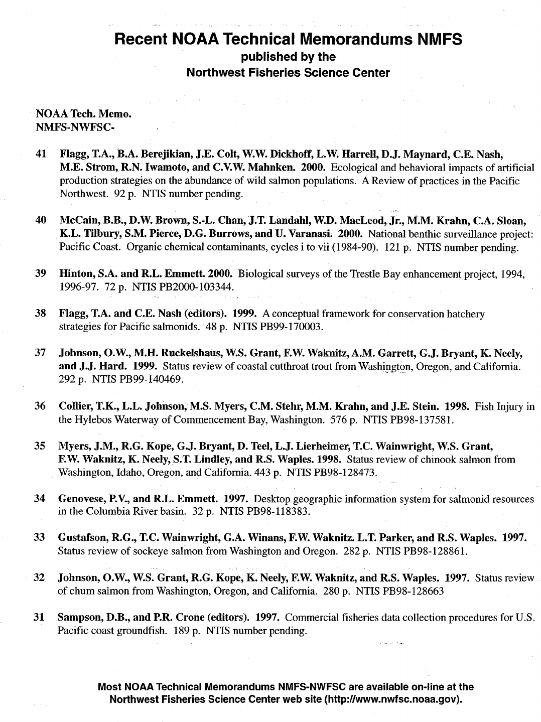
Figure 1. This figure illustrates why subpopulations, populations, and ESUs are likely to have a biological
basis. Each vertical line represents a panmictic (completely interbreeding) group of fish. If the
probability of mating between two individuals is simply a function of distance and the fish are
arranged as in “A,” there will be some biological basis for grouping fish into subpopulations,
populations, and ESUs. If the fish are arranged as “B” depicts, the probability of mating may
still decline with distance, but there are no biologically obvious groupings. The homing
tendencies of Pacific salmon—combined with spatial structure of freshwater spawning
habitat—suggest that most salmon species will resemble the scenario depicted in “A” rather
than that in “B.” The distance measure in this figure may represent simple Euclidean distance
or a more complex measure, such as a metric involving migration barrier permeability.

9
No population, as it is defined here, would ever be a member of more than one ESU, but a single
ESU may contain multiple populations.
Population Definition and Artificial Propagation
The stated purposes of the ESA are to provide a means whereby the ecosystems upon
which endangered and threatened species depend may be conserved, to provide a program for
conserving such species, and to take the steps needed to achieve these purposes (ESA sec. 2[b]).
The ESA's focus is on natural populations and the ecosystems upon which they depend.
Artificial propagation of a listed salmonid species is not a substitute for eliminating the factors
causing or contributing to a species' decline (NMFS 1993).
There are hundreds of artificial propagation programs for salmonids in Washington,
Oregon, Idaho and California. Collectively, they released several hundred million juvenile fish
in the late 1990s (Beamish et al. 1997). Whether by design, as in a supplementation program, or
through unintentional straying, hatchery fish often spawn with natural fish in the wild.
3
In cases
where hatchery fish interbreed with natural fish on spawning grounds and a substantial number
of the spawners are fish of hatchery origin, the naturally spawning component cannot be
considered demographically independent of the hatchery component. In such cases, hatchery
and wild spawning fish are part of the same population. A population that depends upon
naturally spawning hatchery fish for its survival is not viable by our definition (see discussion in
the Appendix sections “Population size,” p. 53 and “Population growth rate and related
parameters,” p. 64). In contrast, it is possible for hatchery-origin and naturally-produced adults
to spawn in the same stream but not be demographically linked to one another. In such cases, the
natural- and hatchery-origin groups of fish constitute separate populations. The natural fish
could be considered a viable population if they meet the VSP criteria.
3
For the purposes of this document, hatchery fish are defined as fish whose parents were spawned in a hatchery,
regardless of parental lineage, and natural fish are defined as fish whose parents spawned in the wild, regardless of
parental lineage. These are definitions for clarity only, and imply nothing about the risks or benefits of hatchery
programs.
10
11
PARAMETERS FOR EVALUATING POPULATIONS
Introduction to Parameters
Population Parameters
Four parameters form the key to evaluating population status. They are: abundance,
population growth rate, population spatial structure, and diversity. NMFS focuses on these
parameters for several reasons. First, they are reasonable predictors of extinction risk (viability).
Second, they reflect general processes that are important to all populations of all species. For
example, many factors influence abundance, (e.g., habitat quality, interactions with other species,
harvest programs, etc.). Many of these factors are species- or ESU-specific. By focusing on
abundance, we can seek general conclusions about an ESU's extinction risk even in the absence
of detailed, species-specific information on all of the factors that influence abundance. Third,
the parameters are measurable. The Appendix discusses specific methods of estimating
population status in the context of each parameter.
Several potential parameters, notably habitat characteristics and ecological interactions,
are not components NMFS uses to define population status, even though they are unquestionably
important to salmonid population viability. The reason these attributes (and others) are not part
of the viability criteria is that their effects are ultimately reflected in the four primary parameters
we do examine. Whenever possible, we discuss how these factors influence a specific
parameter. For example, a population’s spatial structure is to a large degree dictated by habitat
structure, and the spatial structure guidelines reflect this fact. Habitat characteristics and
ecological interactions both tend to be very species-specific, thus, it is well beyond the scope of
this present document to provide guidelines for these factors for every species and life-history
type. However, during the recovery planning process, it will be necessary to explore the explicit
relationships between habitat characteristics, ecological interactions and population parameters
within each ESU.
Guidelines for Each Population Parameter
In order to use the previously mentioned four population parameters to make viability
assessments, NMFS has developed a series of guidelines for each parameter. The guidelines are
drawn from a survey of the conservation biology and salmonid literature. These guidelines are
crude in the sense that they do not take into account the specifics of any particular species or
population. However they are also practical because in many situations, population-specific data
is not available, or a decision about pending action needs to be made before a detailed analysis
can be completed. In these situations, using guidelines may be the best way to evaluate a
population's status. To present the guidelines as concisely as possible, this section includes only
a brief overview of the rationale behind each of them. The bulk of the data, reasoning, and
examples used to create the guidelines are contained in the Appendix. It should be emphasized
12
that these guidelines are based on our interpretation of currently available data and literature. As
with all scientific endeavors, these guidelines can be modified as new data, more rigorous
analysis and clearer interpretations are generated.
Population Size
Small populations face a host of risks intrinsic to their low abundance; conversely, large
populations exhibit a greater degree of resilience. A large part of the science of conservation
biology involves understanding and predicting the effects of population size. All else being
equal, small populations are at greater risk of extinction than large populations primarily because
several processes that affect population dynamics operate differently in small populations than
they do in large populations. These processes are deterministic density effects, environmental
variation, genetic processes, demographic stochasticity, ecological feedback and catastrophes
(Appendix section “Population size,” p. 53). Deterministic effects of population density fall into
two opposing processes: compensation (an increase in productivity with decreasing density) and
depensation (a decrease in productivity with decreasing density). Compensation occurs because
there is an increasing need to compete for limited resources as a population expands to fill (or
exceed) available habitat. The negative relationship between productivity and abundance
observed under compensation can give a population substantial resilience. This resilience occurs
because any decline in abundance is offset by an increase in productivity, which tends to restore
a population to some equilibrium level.
A diverse suite of processes can cause depensatory density effects at small population
sizes. These include the inability of potential mates to find one another and increased predation
rates when predators are unsatiated (see Appendix section “Population growth rate and related
parameters,” p. 64). Depensatory processes at low population abundance (also termed “Allee”
effects) result in high extinction risks for very small populations because any decline in
abundance further reduces the population's average productivity, resulting in a steep slide toward
extinction. Environmental variation can cause small populations to go extinct when chance
events reduce survival or fecundity to low levels for an extended time. The genetic processes
that may negatively affect small populations include diversity loss, inbreeding depression and the
accumulation of deleterious mutations. Demographic stochasticity refers to random events
associated with mate choice, fecundity, fertility, and sex ratios that can create higher extinction
risks in small populations relative to large populations. Ecological feedback is similar to
density-dependent processes, but it emphasizes the role salmon play in modifying their physical
and biological environment and it usually operates at time lags absent from density-dependent
processes. Examples include the contribution of salmon carcasses to riparian zone nutrient
cycles, and the effect of spawning salmon on spawning gravel quality. Both of these processes
can contribute to the success of future salmon generations, but they are only significant at
relatively high population densities. Catastrophes are environmental events that severely reduce
a population size in a relatively short period of time. Because catastrophic events often affect
more than one population and the extinction risks associated with catastrophic failure can be
relatively independent of population size, the effects of catastrophes are considered in the section
on ESU-level viability.

13
We developed the following guidelines in order to assess population viability in light of
the abundance parameter. Note that the ESA=s primary focus is on natural populations in their
native ecosystems, so when we evaluate abundance to help determine VSP status, it is essential
to focus on naturally produced fish (i.e., the progeny of naturally spawning parents). Because
extinction risk depends largely on specific life-history strategies and the local environment,
setting fish abundance criteria will require application of species or population specific
information. For this reason, the following guidelines prescribe factors that need to be
considered but do not provide specific numerical criteria.
Two sets of described guidelines that follow are: Viable Size Guidelines and Critical Size
Guidelines. (Note that these levels are not equivalent to the ESA concepts of Asurvival@ and
Arecovery”; see Appendix section “Applying VSP in the regulatory arena,” p. 33, for more
discussion). A population must meet all of the viable population guidelines to be considered
viable with respect to this parameter. If a population meets even one critical guideline, it would
be considered to be at a critically low level. Also, note that different guidelines are likely to
dominate decisions for different populations. For example, environmental variation (Viable
Guideline 1) will often dictate a larger minimum population size than would genetic concerns
(Viable Guideline 3), but for some populations genetic concerns may predominate.
Population Growth Rate and Related Parameters
Population growth rate (productivity
4
) and factors that affect population growth rate
provide information on how well a population is “performing” in the habitats it occupies during
the life cycle. These parameters, and related trends in abundance, reflect conditions that drive a
population’s dynamics and thus determine its abundance. Changes in environmental conditions,
including ecological interactions, can influence a population's intrinsic productivity or the
environment's capacity to support a population, or both. Such changes may result from random
environmental variation over a wide range of temporal scales (environmental stochasticity). In
this section, however, we are most concerned with measures of population growth and related
parameters that reflect systematic changes in a population's dynamics.
We focus on population growth rate and related parameters as integrated indicators of a
population’s performance in response to its environment. Specific characteristics of a
population’s environment that affect its dynamics, while likely to be similar across populations,
are necessarily deferred to individual case studies. In most cases we are concerned with
estimating a mean parameter that describes some aspect of population dynamics (such as long-
term population growth rate) and with estimating the variance of this parameter. Depending on
the question or parameter of interest, estimates of variance may contribute to descriptions of
uncertainty in parameter estimates, and consequences of decisions based on such estimates may
play an integral role in evaluating the viability of a population. While it is intuitively sensible to
4
We use the terms “population growth rate” and “productivity” interchangeably when referring to production over
the entire life cycle. We also refer to “trend in abundance” which is simply the manifestation of long-term
population growth rate.

14
Viable Population Size Guidelines
1. A population should be large enough to have a high probability of surviving
environmental variation of the patterns and magnitudes observed in the past and
expected in the future. Sources of such variation include fluctuations in ocean conditions
and local disturbances such as contaminant spills or landslides. Environmental variation and
catastrophes are the primary risks for larger populations with positive long-term average
growth rates.
2. A population should have sufficient abundance for compensatory processes to provide
resilience to environmental and anthropogenic perturbation. In effect, this means that
abundance is substantially above levels where depensatory processes are likely to be
important (see Critical Guideline 1 as follows) and in the realm where compensation is
substantially reducing productivity. This level is difficult to determine with any precision
without high quality long-term data on population abundance and productivity, but can be
approximated by a variety of methods.
3. A population should be sufficiently large to maintain its genetic diversity over the long
term. Small populations are subject to various genetic problems, including loss of genetic
variation, inbreeding depression, and deleterious mutation accumulation, that are influenced
more by effective population size than by absolute abundance.
4. A population should be sufficiently abundant to provide important ecological functions
throughout its life-cycle. Salmonids modify both their physical and biological
environments in various ways throughout their life cycle. These modifications can benefit
salmonid production and improve habitat conditions for other organisms as well. The
abundance levels required for these effects depend largely on the local habitat structure and
particular species’ biology.
5. Population status evaluations should take uncertainty regarding abundance into
account. Fish abundance estimates always contain observational error, and therefore
population targets may need to be much larger than the desired population size in order to be
confident that the guideline is actually met. In addition, salmon are short-lived species with
wide year-to-year abundance variations that contribute to uncertainty about average
abundance and trends. For these reasons, it would not be prudent to base abundance criteria
on a single high or low observation. To be considered a VSP, a population should exceed
these criteria on average over a period of time.

15
Critical Population Size Guidelines
1. A population would be critically low if depensatory processes are likely to reduce it
below replacement. The specific population levels where these processes become important
are difficult to determine, although there is theory on mate choice, sex-ratios, and other
population processes that may be helpful in placing a lower bound on safe population levels.
In general, however, small-population depensatory effects depend largely on density rather
than absolute abundance. A species= life-history and habitat structure play large roles in
determining the levels at which depensation becomes important.
2. A population would be critically low if it is at risk from inbreeding depression or
fixation of deleterious mutations. The most important genetic risks for very small
populations are inbreeding depression and fixation of deleterious mutations; these effects are
influenced more by the effective breeding population size than by absolute numbers of
individuals.
3. A population would be critically low in abundance when productivity variation due to
demographic stochasticity becomes a substantial source of risk. Demographic
stochasticity refers to the seemingly random effects of variation in individual survival or
fecundity that are most easily observed in small populations. As populations decline, the
relative influences of environmental variation and demographic stochasticity changes—with
the latter coming to dominate in very small populations.
4. Population status evaluations should take uncertainty regarding abundance into
account. Fish abundance estimates always contain observational error and therefore
population targets may need to be much larger than the desired population size in order to be
confident that the guideline is actually met. In addition, salmon are short-lived species with
wide year-to-year abundance variations that contribute to uncertainty about average
abundance and trends. For these reasons, it would not be prudent to base abundance criteria
on a single high or low observation. To be considered critically low, a population would fall
below these criteria on average over a short period of time.
16
use population growth rate as an indicator of risk and viability, the issue of how to do so in a
quantitative way is still an area of active research.
Estimates of population growth rate (i.e., productivity over the entire life cycle) that
indicate a population is consistently failing to replace itself, are an indicator of increased
extinction risk, no matter what the cause. Some evidence suggests that the major extinction risk
for Pacific salmonids does not arise from stochastic processes but rather from processes (such as
habitat degradation or overharvest) that exert a sustained detrimental effect on a population and
result in a chronically low population growth rate and a negative trend in abundance (Emlen
1995, Ratner et al. 1997). Under this scenario, small population size is a transient stage toward
deterministic extinction. While stochastic processes certainly affect the time to extinction, they
do not affect the likelihood of the outcome.
Although our overall focus is on population growth rate over the entire life cycle, estimates of
stage-specific productivity (particularly productivity during freshwater life-history stages) are
also important for comprehensive evaluation of population viability. Although declines in stage-
specific productivity may not immediately manifest in reduced abundance if offset during other
portions of the life cycle, they may indicate reduced resilience to variation in productivity
elsewhere in the life cycle. As examples, estimates of smolt production provide a measure of
both a population’s potential to increase in abundance (should the recent poor ocean conditions
abate) and a population’s ability to weather future periods of poor ocean conditions. Along
similar lines, changes or shifts in traits that are clearly related to productivity (such as size-at-
return of spawners) may contribute to evaluations of population viability. Such ancillary data
may provide an important source of information that supports more rapid detection of changes in
conditions affecting population growth rate in salmonid populations.
Other measures of population productivity, such as intrinsic productivity and the intensity
of density-dependence, may provide important information for assessing a population’s viability.
For example, a population's intrinsic productivity (defined as its maximum growth rate when free
of density-dependent limitation) partially determines the abundance at which demographic
stochasticity begins to play an important role in determining the fate of the population. Intrinsic
productivity is also a measure of a population's ability to rebound from short-term environmental
or anthropogenic perturbations (resilience). Analyses of extinction models have highlighted the
importance of elucidating the existence and intensity of compensatory density-dependence for
estimating a population's extinction risk (Ginzberg et al. 1990). However, obtaining unbiased
estimates of a population’s intrinsic productivity and the intensity and functional form of
density-dependence affecting a population can be difficult due to autocorrelation and observation
error in the data. Such difficulties hinder the use of these parameters as independent measures of
a population’s viability.
Not surprisingly, the guidelines for population growth rate and related parameters are
closely linked with those for abundance; indeed, the following guidelines are often conditioned
on a population's status in terms of abundance.

17
Population Growth Rate and Related Parameters Guidelines
1. A population’s natural productivity should be sufficient to maintain its abundance above the
viable level. A population meeting or exceeding abundance criteria for viability should, on average,
be able to replace itself. That is, spawner: spawner ratios or cohort-replacement ratios should
fluctuate around 1.0 or above. Natural productivity is typically measured as the ratio of naturally-
produced spawners born in one broodyear to the number of fish spawning in the natural habitat during
that broodyear; population abundance estimates at other life-history stages may also be used,
provided such estimates span the entire life cycle (e.g., smolt to smolt estimates).
2. A viable salmonid population that includes naturally spawning hatchery fish should exhibit
sufficient productivity from naturally-produced spawners to maintain population abundance at
or above viability thresholds in the absence of hatchery subsidy. In a strict sense, this guideline
suggests that the mean Natural Return Ratio (NRR) for a viable population should fluctuate around
1.0, indicating negligible hatchery influence on the population. In a practical sense, the requirement
that a viable population be demographically independent of a hatchery population suggests that a
viable population’s mean NRR not be less than approximately 0.9, but this estimate neglects other
issues related to the influence of hatchery fish on natural production. A viable population should not
exhibit a trend of proportionally increasing contributions from naturally spawning hatchery fish.
3. A viable salmonid population should exhibit sufficient productivity during freshwater life-
history stages to maintain its abundance at or above viable thresholds—even during poor ocean
conditions. A population’s productivity should allow it both to exploit available habitat and exhibit a
compensatory response at low population sizes. When spawner abundance is below the long-term
mean, there should be a corresponding increase in per capita smolt production, even though such an
increase may not suffice to offset declines in marine survival.
4. A viable salmonid population should not exhibit sustained declines in abundance that span
multiple generations and affect multiple broodyear-cycles. “Sustained” declines are those that
continue longer than the typical lag in response associated with a population’s generation time. Thus,
sustained declines differ from rapid transitions between one stable level and another (e.g., changes in
abundance related to large-scale, low frequency environmental forcing such as those related to
oceanic regime shifts). They also differ from short-term, severe perturbations in abundance, such as
those related to strong El Niño events that are followed by relatively rapid recovery.
5. A viable salmonid population should not exhibit trends or shifts in traits that portend declines
in population growth rate. Changes in such traits, such as size and age of spawners, that affect
population growth rate are often more easily and precisely quantified than are changes in abundance
and thus, may provide earlier indication of declining population growth rate. For example, reduced
size of mature individuals in a population may indicate reduced fecundity, lessened ability to reach
spawning grounds, a decreased capacity for constructing redds that are deep enough to resist bed
scour, or other factors that contribute to reduced production of offspring. Likewise, increasing age-at-
return may reduce a population’s intrinsic productivity by exposing adults to greater pre-reproductive
spawning risk.
6. Population status evaluations should take into account uncertainty in estimates of population
growth rate and productivity-related parameters. To estimate long-term trends and spawner-
recruit ratios, it is important to have an adequate time series of abundance. Unfortunately, such time
series, when they exist at all, are often short, contain large observational errors, or both. These
constraints may greatly limit the power of statistical analyses to detect ecologically significant trends
before substantial changes in abundance have occurred.

18
Spatial Structure
When evaluating population viability, it is important to take within-population spatial
structure needs into account for two main reasons: 1) because there is a time lag between
changes in spatial structure and species-level effects, overall extinction risk at the 100-year time
scale may be affected in ways not readily apparent from short-term observations of abundance
and productivity, and 2) population structure affects evolutionary processes and may therefore
alter a population’s ability to respond to environmental change (Appendix section “Spatial
Structure,” p. 90).
5
A population’s spatial structure is made up of both the geographic
distribution of individuals in the population and the processes that generate that distribution.
Spatially structured populations are often generically referred to as “metapopulations,” though
the term metapopulation has taken on a number of different meanings. A population’s spatial
structure depends fundamentally on habitat quality, spatial configuration, and dynamics as well
as the dispersal characteristics of individuals in the population.
Because many of the processes that affect small population extinction risk (e.g., genetic
risks and demographic stochasticity) depend primarily on breeding structure, we will focus on
spawning group distribution and connectivity. Restricting the discussion to spawning groups is
practical for the purposes of evaluating viability, but spatial structure exists during all life-history
stages. Although we focus on breeding structure, it should be noted that with little or no
modification, many of our guidelines could apply to non-breeding spatial structure.
Because freshwater habitat is often quite heterogeneous, salmonids may experience
spawning habitat as discrete “patches” whose quality can vary from highly productive to
unusable. If straying among patches is limited, the population may be divided into
subpopulations. (“Straying” occurs when an individual spawns in a different patch from the one
in which it hatched.
6
) Straying rates form a continuum and, by definition, levels of straying
among subpopulations are higher than those found between populations. The spatial scales that
define habitat patches and subpopulation boundaries are not strictly defined because such
determinations are likely to be species- and population-specific.
5
As one example of how a degraded spatial structure can threaten the viability of a population, consider a
population divided into subpopulations. A population with a high subpopulation extinction rate can persist only if
new subpopulations are founded at a rate equal to the rate at which subpopulations naturally go extinct. If human
activity interferes with the formation of new subpopulations by restricting straying patterns or destroying habitat
patches suitable for colonization, the population will ultimately go extinct as subpopulations blink out one by one.
However, there will be a time lag between the disruption of spatial processes and reductions in the abundance or
productivity of the population because abundance will not necessarily decline until subpopulations start going
extinct.
6
The term “straying” is commonly used in the salmonid literature as we have defined it here. Despite the negative
connotations of the word “straying,” there is no reason to assume that straying is evolutionarily maladaptive. For
non-salmonids, the terms “dispersal” or “migration” are generally used to describe movement away from natal
habitats, resulting in breeding in a non-natal location. However, in the salmonid literature dispersal and migration
often refer to any movement among habitats and straying is the only term restricted to breeding structure.
19
A number of different population structures are possible—depending on habitat patch
physical stability, subpopulation demographic stability, and the levels of straying among patches
(Figure 2). Although there are few data on salmonid breeding spatial structure, what data are
available suggest that the habitat patch size and quality vary greatly within a population. This
indicates that source-sink or island-mainland dynamics might be common. In contrast, there are
few data to support a panmictic or classical metapopulation view of salmonid population spatial
structure (see Appendix section “Spatial Structure,” p. 90 for definitions of these terms). It
should be emphasized, however, that salmonid spatial structure is not well understood, and there
is currently no scientific consensus on what a “typical” spatial structure is. The following
guidelines focus on key processes that are likely to be important in maintaining a viable spatial
structure, regardless of population type.
Diversity
Several salmonid traits exhibit considerable diversity within and among populations.
This variation has important effects on population viability (Appendix section “Diversity,” p.
101). Some of these varying traits are anadromy, morphology, fecundity, run timing, spawn
timing, juvenile behavior, age at smolting, age at maturity, egg size, developmental rate, ocean
distribution patterns, male and female spawning behavior, physiology and molecular genetic
characteristics. Of these traits, some (such as DNA or protein sequence variation) are completely
genetically based, whereas others (such as nearly all morphological, behavioral, and life-history
traits) usually vary as a result of a combination of genetic and environmental factors.
In a spatially and temporally varying environment, there are three general reasons why
diversity is important for species and population viability. First, diversity allows a species to use
a wider array of environments than they could without it. For example, varying adult run and
spawn timing allows several salmonid species to use a greater variety of spawning habitats than
would be possible without this diversity. Second, diversity protects a species against short-term
spatial and temporal changes in the environment. Fish with different characteristics have
different likelihoods of persisting—depending on local environmental conditions. Therefore, the
more diverse a population is, the more likely it is that some individuals would survive and
reproduce in the face of environmental variation. Third, genetic diversity provides the raw
material for surviving long-term environmental changes. Salmonids regularly face cyclic or
directional changes in their freshwater, estuarine, and ocean environments due to natural and
human causes, and genetic diversity allows them to adapt to these changes.
Any actions that affect basic demographic and evolutionary processes (e.g., patterns of
mutation, selection, drift, recombination, migration, and population turnover) have the potential
to alter a species’ diversity. For example, straying and gene flow among populations strongly
influence diversity within and among populations. Gene flow refers to the movement of genes
from one population to another and results from strays that successfully reproduce. There are a
number of ways in which human actions could substantially alter patterns of straying and,
therefore, potentially alter patterns of diversity and adaptation among salmonid populations. For
example, blocking migration corridors with dams and dewatering rivers can prevent salmonids
from homing and thus increase the rate of straying into other populations.

20
homogeneous panmictic population
patchy panmictic population
“classical”
metapopulation
Low survival years -
single panmictic
population
Moderate survival year -
source sink population
High survival years -
structured population
Panel B: Temporal changes in
population structure
Panel A: “Traditional”
classification of population
structure
Panel C: Static vs. dynamic habitat
Static habitat
Dynamic habitat
Time 1 Time 3Time 2
Time 1 Time 3Time 2
structured populaton
with no extinctions
source-sink population
island-mainland population
Figure 2. Theoretical types of spatially structured populations. Panel A shows a “traditional” type
classification scheme that does not consider correlated environmental effects that impact all
subpopulations nor does it explicitly consider the physical dynamics of the habitat patches
themselves. The circles indicate habitat patches, with the size of the circle indicating the size or
capacity of the patch, and the degree of shading indicating the density of the subpopulation—
white indicating an empty patch and black indicating a high density patch. The arrows indicate
levels of migration, with thick arrows indicating high migration; thin arrows moderate migration,
and dashed arrows indicating intermittent migration. Panel B shows how spatial structure may
oscillate over time as a result of correlated environmental changes in survival or productivity
among subpopulations. Correlated environmental changes might result, for example, from annual
variation in ocean survival that affects all subpopulations. Panel C shows two potential habitat
patterns. In a static habitat, the location of suitable patches remains constant over time, though
patches may or may not always be occupied. In a dynamic habitat, the location of suitable habitat
continually changes, and so the location of subpopulations must also change.

21
Spatial Structure Guidelines
1. Habitat patches should not be destroyed faster than they are naturally created. Salmonid
habitat is dynamic, with suitable habitat being continually created and destroyed by natural processes.
Human activities should not decrease either the total area of habitat OR the number of habitat patches.
This guideline is similar to the population growth rate criterion—i.e., a negative trend has
deterministically negative affects on viability—though the relationship between decreasing number of
patches and extinction risk is not necessarily linear.
2. Natural rates of straying among subpopulations should not be substantially increased or
decreased by human actions. This guideline means that habitat patches should be close enough
together to allow appropriate exchange of spawners and the expansion of the population into under-
used patches, during times when salmon are abundant (see Guideline 3). Also, stray rates should not
be much greater than pristine levels, because increases in stray rates may negatively affect a
population’s viability if fish wander into unsuitable habitat or interbreed with genetically unrelated
fish.
3. Some habitat patches should be maintained that appear to be suitable or marginally suitable,
but currently contain no fish. In the dynamics of natural populations, there may be time lags
between the appearance of empty but suitable habitat (by whatever process) and the colonization of
that habitat. If human activity is allowed to render habitat unsuitable when no fish are present, the
population as a whole may not be sustainable over the long term.
4. Source subpopulations should be maintained. Some habitat patches are naturally more productive
than others. In fact, a few patches may operate as highly productive source subpopulations that
support several sink subpopulations that are not self-sustaining. Protecting these source patches
should obviously be of the highest priority. However, it should be recognized that spatial processes
are dynamic and sources and sinks may exchange roles over time
5. Analyses of population spatial processes should take uncertainty into account. In general, there
is less information available on how spatial processes relate to salmonid viability than there is for the
other VSP parameters. As a default, historic spatial processes should be preserved because we
assume that the historical population structure was sustainable but we do not know whether a novel
spatial structure will be.

22
Diversity Guidelines
1. Human-caused factors such as habitat changes, harvest pressures, artificial propagation, and
exotic species introduction should not substantially alter variation in traits such as run timing,
age structure, size, fecundity, morphology, behavior, and molecular genetic characteristics.
Many of these traits may be adaptations to local conditions, or they may help protect a population
against environmental variation. A mixture of genetic and environmental factors usually causes
phenotypic diversity, and this diversity should be maintained even if it cannot be shown to have a
genetic basis.
2. Natural processes of dispersal should be maintained. Human-cased factors should not
substantially alter the rate of gene flow among populations. Human caused inter-ESU stray rates
that are expected to produce (inferred) sustained gene flow rates greater than 1% (into a population)
should be cause for concern. Human caused intra-ESU stray rates that are expected to produce
substantial changes in patterns of gene flow should be avoided.
3. Natural processes that cause ecological variation should be maintained. Phenotypic diversity can
be maintained by spatial and temporal variation in habitat characteristics. This guideline involves
maintaining processes that promote ecological diversity, including natural habitat disturbance regimes
and factors that maintain habitat patches of sufficient quality for successful colonization.
4. Population status evaluations should take uncertainty about requisite levels of diversity into
account. Our understanding of the role diversity plays in Pacific salmonid viability is limited.
Historically, salmonid populations were generally self-sustaining, and the historical representation of
phenotypic diversity serves as a useful “default” goal in maintaining viable populations.
23
Integrating the Parameters and Determining Population Status
The key parameters used to determine whether a population is likely to enjoy long-term
viability are abundance, population growth rate, population spatial structure, and diversity. As a
rule, these four population attributes cannot be viewed entirely independently. For example, the
value ranges for population growth rate considered necessary for a viable population clearly
depend on the population’s abundance (Appendix section “Population growth rate and related
parameters,” p. 64). Making an overall determination of population status will usually require
some method of integrating the parameters.
We believe the guidelines for each of the four parameters (p. 14, 15, 17, and 21) describe
the actions needed to maintain salmonid population viability over a 100-year period.
Nevertheless, because the guidelines we provide are qualitative, modeling tools (such as
population viability analyses) may prove useful in exploring tradeoffs between parameters such
as population size and productivity. For example, a model could be constructed that examines
the extinction dynamics of a salmonid population under different population size scenarios and
spawner-to-recruit ratios in order to combine a population’s characteristics and estimate their
effects on viability. Similarly, a structured modeling approach could explore the effects on
population viability that different subpopulation numbers, abundance, and distribution would
have.
24
25
ESU VIABILITY
Introduction
To help understand basic salmonid biology and formulate priorities for salmon
management, it is useful to explore the extinction risks that individual population’s experience.
However, in many cases it is also important to consider how these individual population risks
relate to sustainability of larger conservation units such as Genetic Diversity Management Units
(GDMU, defined by WDFW), Major Ancestral Lineages (defined by WDFW), or Gene
Conservation Groups (defined by ODFW). The ESA is ultimately concerned with the extinction
of any entity that qualifies as a “species” under the ESA, which for vertebrate animals includes
species, subspecies, or “distinct population segments.” According to NMFS policy, groups of
salmon populations that represent Evolutionarily Significant Units (ESUs) of the species as a
whole are considered distinct population segments and hence, “species” under the ESA. The
goal of this section of the document is to discuss factors that should be evaluated when
determining the numbers and distribution of VSPs needed to sustain larger conservation units
such as ESUs. Like the section on population viability, this section describes only qualitative
guidelines for determining ESU viability. The assumption is that in order to determine the
necessary population numbers and distribution in a given ESU, case-specific information will be
required. Appendix section “ESU Viability Guidelines” (p. 127) provides a more detailed
rationale for the guidelines.
Number and Distribution of Populations in a Recovered ESU
By definition, a VSP has a negligible risk (over a time scale of 100 years) of going
extinct as a result of genetic change, demographic stochasticity, or normal levels of
environmental variability. If these were the only factors influencing viability, a single VSP
would be enough to ensure the survival of an entire ESU. However, three additional factors need
to be considered in relating VSPs to viable ESUs: 1) catastrophic events, 2) long-term
demographic processes, and 3) long-term evolutionary potential. Catastrophic events are sudden,
rare occurrences that severely reduce or eliminate an entire population. These events fall outside
the scope of the “normal” temporal and spatial scales of environmental variation considered
when evaluating VSPs. Long-term demographic processes involve extinction and recolonization
of entire populations at time scales greater than 100 years. The concern about long-term
evolutionary potential centers on the role diversity plays in ESU viability over time scales that
are generally greater than 100 years.
In addition to biological considerations, the ESA defines an endangered species as a
species that is “…in danger of extinction in all or a significant portion of its range.” The ESA
does not define “significant portion of the range” and there is no indication that the phrase is
meant to be (or can be) defined entirely in scientific terms. As noted in the appendix section
“Applying VSP in the regulatory arena” (p. 33), it will probably be necessary to define “a
significant portion of the range” in both scientific and policy terms. Scientifically, a significant

26
ESU Viability Guidelines
1. ESUs should contain multiple populations. If an ESU is made up of multiple populations, it is less
likely that a single catastrophic event will cause it to become extinct. Also, ESUs may function as
“metapopulations” over the long term and the existence of multiple populations would be necessary
for the operation of sustainable population-level extinction/recolonization processes. In addition,
multiple populations within an ESU increase the likelihood that a diversity of phenotypic and
genotypic characteristics will be maintained, thus allowing natural evolutionary processes to operate
and increasing the ESU’s viability in the long term. Obviously, this guideline does not apply to ESUs
that appear to contain a single population (e.g., Lake Ozette sockeye). In ESUs containing a single
population Guideline 6 becomes increasingly important.
2. Some populations in an ESU should be geographically widespread. Spatially correlated
environmental catastrophes are less likely to drive a widespread ESU to extinction. This guideline
also directly relates to the ESA mandate of protecting a species in a “significant portion of (its)
range.”
3. Some populations should be geographically close to each other. On long temporal scales, ESUs
may function as “metapopulations” and having populations geographically close to one another
facilitates connectivity among existing populations. Thus, a viable ESU requires both widespread
(Guideline 2) AND spatially close populations.
4. Populations should not all share common catastrophic risks. An ESU containing populations that
do not share common catastrophic risks is less likely to be driven to extinction by correlated
environmental catastrophes. Maintaining geographically widespread populations is one way to
reduce risk associated with correlated catastrophes (Guideline 2), but spatial proximity is not the only
reason why two populations could experience a correlated catastrophic risk.
5. Populations that display diverse life-histories and phenotypes should be maintained. When an
ESU’s populations have a fair degree of life-history diversity (or other phenotypic diversity), the ESU
is less likely to go extinct as a result of correlated environmental catastrophes or changes in
environmental conditions that occur too rapidly for an evolutionary response. In addition, assuming
phenotypic diversity is caused at least in part by genetic diversity, maintaining diversity allows
natural evolutionary processes to operate within an ESU.
6. Some populations should exceed VSP guidelines. Larger and more productive (“resilient”)
populations may be able to recover from a catastrophic event that would cause the extinction of a
smaller population. An ESU that contains some populations in excess of VSP threshold criteria for
abundance and population growth rate is less likely to go extinct in response to a single catastrophic
event that affects all populations. It is important to note that the abundance guidelines do not take
catastrophes into account. This guideline is particularly relevant if an ESU consists of a single
population.
7. Evaluations of ESU status should take into account uncertainty about ESU-level processes. Our
understanding of ESU-level spatial and temporal process is very limited. ESUs are believed to have
been historically self-sustaining and the historical number and distribution of populations serves as a
useful “default” goal in maintaining viable ESUs.
27
portion of the range will be determined by evaluating the risks to ESU persistence at a number of
time scales, including those longer than 100 years.
Populations Not Meeting VSP Guidelines
After conducting a viability analysis, a group of fish considered to be an independent
population under the VSP definition might not appear to meet the VSP guidelines. There are a
number of reasons why a population may appear non-viable. Some of these reasons involve a
correct assessment of population status, while others involve some error in assessment.
Understanding why a population is not considered viable, and the potential mistakes in reaching
that conclusion is important in assessing ESU viability.
A group of fish could be mislabeled as not viable if it has been misidentified as an
independent population and should actually be considered to be a subpopulation of a larger
group. Population and subpopulation designations fall along a continuum of reproductive
isolation, and in borderline cases it is difficult to determine population structure for a group of
fish (see “Identifying populations,” p. 51). Ambiguity about population structure may often be a
challenging reality in evaluating ESU-level status.
Even if population boundaries are appropriately identified, a population may still be
inaccurately characterized as inviable. Evaluating population status with limited data is a
difficult task and errors are inevitable. This is particularly true if a population is in some way
unusual and comparing it to other salmonid populations would be misleading.
Despite challenges assessing population boundaries and population viability, the
conclusions that a population is not viable may be correct. In many areas, human activities have
so ffected individual survival and fecundity that it is difficult or impossible for an independent,
viable population to become established.
An interesting situation exists when a population is independent, but would not be
considered viable (i.e., it would not have a negligible risk of extinction in 100 years), even under
pristine conditions. There are a number of reasons why independent populations might not be
viable, even under pristine conditions. For example, a population may be particularly prone to
catastrophic events or large environmental fluctuations, as would be expected on the margins of
a species’ range. Alternatively, a population may be so small naturally that it is unlikely to
persist for 100 years. Truly independent but inviable populations may periodically be generated
by strays from viable populations, and these relatively ephemeral populations would be part of
ESU-level metapopulation processes. These types of populations will have to be taken into
account on a case-by-case basis when an ESU’s status is being evaluated. They may be quite
important to an ESU’s viability if it functions as a large metapopulation with population turnover
occurring at relatively short time scales. In an ESU consisting primarily of populations that
would be viable under pristine conditions, the potentially viable populations would likely be
given highest conservation priority.
28
29
IMPLEMENTING THE VSP GUIDELINES
Introduction
ESA recovery plans are required to provide objective, measurable criteria for determining
when delisting is warranted (ESA Sec. 4[f]). Delisting criteria are also useful in performing
other ESA related activities, such as consultations, permits, habitat conservation plans, and
regulations (see “Applying VSP in the regulatory arena,” p. 33). The VSP guidelines presented
in this document are intended to guide the development of specific delisting/recovery criteria for
Pacific salmon ESUs.
The guidelines presented here are intentionally general so they can be applied equally
across the wide spectrum of life-history diversity, habitat conditions, and meta-population
structures represented by Pacific salmon. It would be irresponsible to propose specific numerical
criteria to be applied uniformly across all Pacific salmon ESUs; specific critieria should take into
account species-specific life-history traits and local habitat structure. For example, population
structure and abundance criteria for sockeye salmon spawning in a north Washington coastal
lake would be expected to differ substantially from those for steelhead spawning in intermittent
streams on the Southern California coast. In addition, the type and amount of information
available varies considerably by species and region, which will influence the emphasis placed on
the various guidelines in specific applications.
Practical Application
Given the generality of these guidelines, it is important to consider how they will be
applied in practice to develop biological delisting criteria. NMFS envisions this to be a three-
step process:
1) Define populations within each ESU.
2) Identify VSP criteria for each population.
3) Identify ESU-wide delisting criteria based on the VSP population criteria.
These steps are discussed in a draft guidance document for technical recovery teams (NMFS
2000a).
Uncertainty, Precaution, and Adaptive Management
A main concern in translating the guidelines into specific criteria will be the degree of
uncertainty in much of the relevant information. There are two widely recognized principles for
approaching resource conservation under uncertainty that should be applied in application of
VSP: the precautionary approach and adaptive management.

30
The precautionary approach requires managers to implement conservation measures even
in the absence of scientific certainty regarding risks. This approach is widely recommended in
harvest management. For example, NMFS' National Standard Guidelines for the Magnuson-
Stevens Fishery Conservation and Management Act (50 CFR Part 600, FR 63:24212-24237)
specifiy use of a precautionary approach both for the specification of optimum yield (OY,
National Standard 1) and in managing bycatch (National Standard 9). The precautionary
approach is also clearly defined in the FAO Code of Conduct for Responsible Fisheries (see
discussion in Ch. 5 of Committee on Ecosystem Management for Sustainable Marine Fisheries
1999). We believe this approach to be equally appropriate in other management areas. An
application to habitat is discussed briefly by the Committee on Protection and Management of
Pacific Northwest Anadromous Salmonids (1996). In practical terms, a precautionary approach
results in shifting the burden of proof, putting that burden in favor of resource conservation
rather than direct economic benefit. For quantitative criteria, this can be accomplished through
careful consideration of appropriate levels of statistical confidence and power in comparing
estimated population parameters to criteria.
Adaptive management encourages the design of management policies designed to
improve the resource knowledge base through active or passive experimentation (Holling 1978,
Walters 1986). General principles for designing adaptive policies are described by Walters
(1986). The Committee on Protection and Management of Pacific Northwest Anadromous
Salmonids (1996) discussed specific applications to salmon management under the ESA.
Interim Application
We have emphasized the role of technical recovery teams in establishing specific criteria
for listed ESUs. However, management actions still need to be taken while recovery teams are
being formed and recovery goals are being developed. It may be useful for agencies involved in
such actions to establish interim criteria that will be used until recovery plans are adopted. Such
interim criteria should be based on a careful consideration of the precautionary principle and
adaptive management methods. Often, a full review of population structure will not be possible
within management time frames. In such situations, agencies might adopt population definitions
already available in state wild fish conservation reports or similar stock-based management
plans, provided these definitions are reasonably consistent with the VSP population definition.
Interim population definitions and criteria should be based on precautionary application of the
VSP criteria. Strong precaution at this stage will help ensure a rapid start along the road to
recovery and that no significant parts of the ESU are lost before the full recovery plan is
implemented. At the ESU level, we suggest that during this interim period, actions should be
taken such that all populations with the ESU retain the potential to achieve viable status. This
would ensure that all parts of the system are maintained until a final plan establishes ESU-level
criteria. Adaptive management should be emphasized to provide improved information and to
allow for changing goals and management strategies as recovery plans are developed.
31
Examples
The VSP guidelines are currently being applied in formal ESA recovery planning by the
Puget Sound and Willamette/Lower Columbia technical recovery teams, but products from these
groups are not yet available. (The only example of applying these guidelines is the work of a
multi-agency work group preparing a “Quantitative Analytical Report” for upper Columbia
River steelhead and spring chinook salmon [Ford et al. 1999a].)
32
33
APPENDIX
Applying VSP in the Regulatory Arena
This document focuses on scientific/biological aspects of populations and more complex
conservation units, but it is also intended to be useful for a wide variety of applications in the
conservation and management of salmonids—at local, state, national, and international levels.
Typically these applications require relating biological principles to regulatory language
involving terms such as “survival,” “recovery,” and “extinction.” For example, implementation
of the federal ESA requires determining when listed species are at risk of extinction or
endangerment, when they have reached a level at which they can be delisted, and when they are
likely to be jeopardized by a proposed action. This document defines another term, population
viability, as a negligible probability of extinction over a 100-year time frame. Although 100
years is a commonly-used time horizon for evaluating extinction risk (or persistence probability)
in the field of conservation biology, it does not relate directly to any particular regulatory
language described previously. It is beyond the scope of this document to make this formal
linkage. Nevertheless, it is useful to briefly review the key regulatory language for federal ESA
implementation and to comment in general on how such linkages might be made.
Listing Criteria
The ESA (“Number and distribution of populations in a recovered ESU,” p. 25) defines
an “endangered” species as “any species which is in danger of extinction throughout all or a
significant portion of its range.” A “threatened” species is “any species which is likely to
become an endangered species within the foreseeable future throughout all or a significant
portion of its range.” From the perspective of applying VSP to entire ESUs, the relevant terms
are “likely to become,” “foreseeable future,” and “significant portion of its range.” Neither
NMFS nor the U.S. Fish and Wildlife Service has defined any of these terms in a policy context.
Thompson (1991) reviewed existing extinction models and rules of thumb for evaluating
population status and noted that although selecting values for extinction probability (p) and time
horizon (t) is only partially a biological exercise (and therefore there is no intrinsically “right”
answer), conservation biologists commonly choose the values p = 0.5 and t = 100 years to
represent an endangerment threshold. Thompson also suggested that a reasonable interpretation
of a “likely” event is one that has at least a 50% chance of occurring. Defining “foreseeable
future” is less intuitive. Thompson suggested that something on the order of 10 years might be
appropriate, but a number of other interpretations are possible.
Because ESUs are considered “species” under the ESA, and a species can be listed if it is
threatened or endangered in “all or a significant portion of its range”, it is essential to take the
meaning of this phrase into consideration when applying VSP guidelines to entire ESUs. The
common scientific usage of “statistical significance” does not appear to be pertinent here; rather,
the relevant meaning of “significant” must be more along the lines of “important; of
consequence” (Random House Dictionary, 2nd Edition). “Range” has an obvious geographic
34
interpretation, and the sections of this document that discuss population abundance and
geographic distribution are relevant in this context. In addition, we believe it is important to
consider other aspects of the “range” concept when evaluating ESU viability; these might
include ecological diversity, life-history diversity, and genetic diversity. The “Diversity” section
(p. 19) discusses long-term ecological and evolutionary processes and thus is directly relevant to
this concept of “range.” In summary, because the process of determining what constitutes a
“significant portion” of a species’ range is only partially based on biological considerations, the
technical definitions of these terms are of limited use.
Recovery
NMFS and the U.S. Fish and Wildlife Service define recovery under the Act to be
“improvement in the status of a listed species to the point at which listing is no longer
appropriate” under the ESA (50 CFR S402.02). This indicates that there is a strong connection
between listing and delisting criteria. Thus, the biological criteria used to make listing
determinations should also be used to evaluate recovery. However, there are several reasons
why listing and delisting criteria values should not be identical. First, if simple threshold values
were used for setting criteria, a species that fluctuates around the critical value might require
repeated listing and delisting actions even though its status had changed relatively little. Second,
listing and delisting criteria require that population trends (and other factors) are considered in
addition to abundance, and trends are expected to differ between declining and recovering
populations. Finally, delisting should occur only in conjunction with an approved,
comprehensive recovery plan that lays out conservation measures that address the factors that led
to the initial decline and those that impede recovery. The preceding discussion applies to
recovery as the ESA defines it. In addition, the NMFS, states, tribes, and many other
stakeholders have an interest in recovering salmon populations to the point at which they can
support sustainable harvest or other “broad sense” recovery goals (e.g., to produce fully
functional ecosystems). Recognizing this, NOAA has made the following commitment (Garcia
1998):
It is our policy that the recovery of salmonid populations must achieve two goals: 1) Restore
salmonid populations to the point where they no longer require the protection of the ESA, and
2) restore salmonid populations to a level that allows meaningful exercise of tribal fishing rights.
We see no conflict between the statutory goals of the ESA and the federal trust responsibilities to
Indian tribes. Rather, the two federal responsibilities complement one another.
Furthermore, NOAA has an obligation under the Sustainable Fisheries Act to restore
depleted populations to optimal levels of abundance and productivity. The VSP concept can be
used to inform management decisions in this context. If, for example, it were a management
objective to ensure a population's sustainability while providing for a specified level of harvest,
VSP guidelines could be used to help determine the population abundance, productivity,
diversity, and structure that would be required to achieve this objective.
35
Jeopardy
Federal agencies cannot undertake or authorize an action that is “likely to jeopardize the
continued existence” of a species listed under the ESA (ESA Section 7). Joint NMFS-USFWS
regulations define “jeopardize the continued existence of” to mean “to engage in an action that
reasonably would be expected, directly or indirectly, to reduce appreciably the likelihood of both
the survival and recovery of a listed species in the wild by reducing the reproduction, numbers or
distribution of that species” (50 CFR S402.02). In the context of jeopardy, “survival” is “the
condition in which a species continues to exist into the future while retaining the potential for
recovery” (USFWS and NMFS 1998). The precise meaning of “into the future” is not defined,
but it clearly represents something short of the time frames associated with ESA recovery. In
contrast, the concept of “long-term survival,”, as considered in long-term conservation plans,
does not differ substantially from the concept of ESA recovery because both require a high
probability that the species will persist for substantial periods of time (Waples 1997). Thus
“jeopardy” currently lacks a precise biological definition; instead, it is defined in a legal context
that introduces several secondary terms that do not have precise biological definitions.
Therefore, it is not surprising that it has been difficult to develop and apply jeopardy standards.
We will need clearer definitions or interpretations of these secondary terms before we can forge
a formal link between VSP and jeopardy determinations. Nevertheless, it is useful to consider
the risks that affect listed species’ survival because that is often the major factor in jeopardy
determinations.
For purposes of this discussion, we assume that risks to a species may constitute jeopardy
if the risks pose threats to short- or long-term species survival. Some jeopardy evaluations have
made use of “critical” thresholds that trigger strong management actions if exceeded. In most
cases, a “critical” status means that a population has a non-negligible probability of going extinct
over a relatively short time period (e.g., 10 years). A problem with implementing jeopardy
standards has been the difficulty in assessing the cumulative effects of a number of actions that
have impacts which are necessarily evaluated at small spatial and temporal scales. Using the
VSP concept as a framework should help determine the net effects “jeopardy” actions have on
population or ESU viability.
Relationship of VSP to Other Concepts
Relationship to Minimum Viable Population Concepts
The VSP concept is closely related to the concept of a minimum viable population
(MVP) (Shaffer 1981). Soulé (1987) defines an MVP as a population that is sufficiently
abundant and well adapted to its environment that it will persist in the long term without
significant artificial demographic or genetic manipulations. Meffe and Carroll (1994) define an
MVP as “the smallest isolated population size that has a specified percent chance of remaining
extant for a specified period of time in the face of foreseeable demographic, genetic, and
environmental stochasticities, plus natural catastrophes.” The MVP concept has been used in a
36
number of conservation applications, from reserve design to extinction risk analyses (see reviews
in Soulé 1987).
Though the VSP concept shares many features with the MVP concept, the two differ in
several important ways. First, abundance has historically been the primary factor in defining an
MVP (Soulé 1987). A VSP, on the other hand, is defined by a variety of parameters, including
population growth rate, population spatial structure, and diversity. Second, although we suggest
minimal thresholds for a VSP (see appendix sections “Population growth rate and related
parameters” through “Viable ESUs,” p. 64-127), any population that meets or exceeds these
thresholds is considered viable. In other words, VSPs include not just minimally viable
populations, but more robust populations as well. Finally, the VSP concept is specifically
tailored for use with Pacific salmonids and thus emphasizes parameters and criteria that are
particularly relevant to this group of species.
Relationship to Quantitative Population Viability Analysis
Population viability analysis (PVA) is a widely-used tool for estimating extinction
probabilities (Soulé 1987, Caughley and Gunn 1996) and it is being increasingly applied to
salmon populations (Spencer 1999). However, there are presently no models that completely
represent the various risks facing salmonid populations. The VSP concept is intended to provide
useful benchmarks for evaluating actions, such as harvest or artificial propagation, that directly
affect natural populations and for which incremental increases in extinction risk may be difficult
or impossible to accurately quantify. The VSP concept is not intended to replace quantitative
risk models in situations where these models can be appropriately used, and the concept could be
used in conjunction with quantitative models in some cases. For example, the effects of harvest
on abundance (one parameter of a VSP) may be relatively easy to quantify and model, but the
simple life-cycle models usually used to evaluate and set harvest levels, often are inadequate for
accurately estimating extinction risk. The VSP concept, by determining the level of abundance
(among other parameters) necessary for long-term survival, could be used in conjunction with a
quantitative life-cycle harvest model to determine if a specific harvest action is likely to cause a
population to fall below VSP parameters. Until extinction risk can be accurately estimated under
a variety of scenarios for Pacific salmonid populations and ESUs, the VSP concept will be of
great help in assessing actions that directly or indirectly affect population viability.
Relationship to Properly Functioning Conditions
Although viable salmonid populations clearly require high quality freshwater habitat, this
document focuses on population processes and does not attempt to establish the relationship
between particular habitat attributes and population viability. This is appropriate given the
purpose of this document, which is to provide a foundation for setting recovery goals of listed
ESUs. These goals will be based on current and projected status of the fish populations, not on
the presence or absence of particular habitat attributes. Of course, assessments of the current and
future status of the population will take habitat attributes into consideration, but the fish
themselves are the ultimate indicator of whether or not the population continues to be in danger
of extinction.
37
Understanding the relationship between freshwater habitat quantity and quality and
population viability is critical in developing recovery plans and in determining the impact of
proposed land use activities on fish survival. To assess the effects of actions that may adversely
modify a species' habitat, NMFS uses the concept of “Properly Functioning Condition” (PFC,
NMFS 1999). PFC defines, based on currently available knowledge, the freshwater spawning
and rearing habitat conditions necessary for the long-term survival of Pacific salmon
populations. To evaluate the effects of specific habitat actions, NMFS uses analytical tools (e.g.,
the Matrix of Pathways and Indicators, NMFS 1996) to determine whether an action will
maintain, restore, or degrade the values of the parameters that describe properly functioning
conditions. The incremental increase in extinction risk from a habitat action is not estimated per
se. Instead, PFC describes the freshwater habitat conditions needed for long-term species
survival, and subsequent actions are evaluated based on how they affect the habitat conditions.
Defining PFC is an ongoing process that will continue to undergo revision, as more scientific
data become available. A particular challenge in developing PFC guidelines is relating habitat
actions at a variety of spatial scales to population-level responses.
Relationship to the Sustainable Fisheries Act (SFA) and Maximum
Sustainable Yield (MSY)
In addition to ESA responsibilities, NMFS has responsibility for administering marine
fisheries under the Magnuson-Stevens Fishery Conservation and Management Act, as amended
by the Sustainable Fisheries Act of 1996 (SFA). Important concepts in the SFA that relate to
population viability include optimum yield (OY), overfishing, and essential fish habitat (EFH).
The Pacific Fishery Management Council recently introduced Draft Amendment 14 to the
Pacific Coast Salmon Plan (PFMC 1999), which incorporates the SFA provisions into Pacific
salmon ocean fisheries management. In developing the VSP concept, we have made no
assumptions regarding the allowable level of harvest for listed salmon populations. In this
regard, harvest is treated similarly to other management factors that influence salmon
populations (i.e., hatcheries, habitat, and hydropower). However, we believe the VSP concept is
consistent with the intent of the SFA provisions because populations achieving viable status will
likely provide greater ocean and freshwater harvest opportunities.
The VSP guidelines have no explicit relationship to maximum sustainable yield (MSY)
analyses for a number of reasons. First, MSY generally deals only with population numbers and
VSP takes into account other parameters that affect population viability such as spatial structure
and diversity. Also, VSP is concerned with extinction risk, not with setting harvest levels. In
addition, VSP analyses focus on estimating extinction risk and examining stochastic processes at
small population sizes, issues that are generally not covered in MSY estimates. Assuming MSY
is actually being achieved, a wild population harvested at MSY is, by definition, sustainable
(VSP)—provided that the time horizon of MSY is the same as VSP and the MSY estimate takes
into account all the factors affecting viability, such as genetic diversity and spatial structure.
38
Relationship to Other Conservation Assessment Approaches
A number of other approaches are used to assess risks at the species and population
levels. One of the most widely used is that of the International Union for the Conservation of
Nature (IUCN) for its Red Book (IUCN Species Survival Commission 1994). The IUCN rates
species on the basis of five general criteria: Population reduction, limited extent of occurrence
combined with decline or fluctuation, low population abundance with continuing decline,
extremely low abundance, and quantitative viability analysis. These criteria differ from ours in
three respects: 1) IUCN criteria are applied to a species as a whole, not to individual populations,
2) some of the IUCN criteria link abundance or geographic range with decline (analogous to our
“population growth rate”) while our criteria treat abundance and productivity separately, and
3) we explicitly treat population structure and diversity as separate parameters. Allendorf et al.
(1997) proposed criteria for Pacific salmon that were similar to the IUCN criteria, but adapted
them specifically to the purpose of ranking threats to individual populations rather than
classifying them as individual risk categories (see also Currens et al. 1998, Wainwright and
Waples 1998). The specific criteria values proposed here differ somewhat from both the IUCN’s
and those developed by Allendorf et al. because they serve a different purpose: we define criteria
that are appropriate for classifying populations as viable, sub-viable, or critical within the context
of broader ESUs and in concert with the requirements of the ESA. Our criteria differ further
from the IUCN’s because we restrict them to a single genus, rather than developing them for all
organisms.
Identifying Populations
Introduction to Identifying Populations
Conceiving of and defining a population is relatively straightforward in a theoretical
sense. It is another matter to identify populations in nature. In practice, information is limited
about the distribution, local abundance, and migratory patterns of a species during their life
cycle. For Pacific salmonids, whose life history occurs in such diverse habitats as freshwater
tributary streams and ocean environments, the challenges associated with delimiting population
boundaries are many. Nevertheless, a number of different types of information can be used to
indicate the geographic or temporal boundaries of a salmon breeding population. This section
has two main parts. First we briefly outline the kinds of information that can be used to help
identify salmon populations. Second, we review approaches to identifying salmonid populations
used in management at state, tribal, and federal levels.
Types of Information Used in Identifying Populations
The different types of population boundary indicators discussed in this section apply to
all levels of structure, from substructure within populations to the structure of populations within
ESUs. Most of the methods described in this section can be used to generate a nested hierarchy
of spatial scales over which some level of indicator subdivision can occur. There is spatial
39
pattern at many scales in the biological and geographical data relevant to salmon, the challenge
to scientists managing salmon under the Endangered Species Act is to identify the appropriate
groupings of salmon that are most useful for predicting the long-term persistence of populations
and ESUs. Making the leap from identifying distinct groups of fish based on similarity of
characteristics to identifying distinct populations depends critically on how independent the
groups of fish are. As we have defined populations in this document, a group of fish is
considered an independent population if migrants from other groups do not appreciably affect the
population dynamics or extinction probability of the focal group (see discussion in “Population
Concepts,” p. 4).
Evidence for independent populations
The best evidence for identifying populations comes from information on a group’s
extinction probability and the degree to which its population dynamics are independent of those
of any other group. Such evidence could come from direct observations of trends in abundance
or productivity from groups of fish with known inter-group stray rates. If the dynamics or
extinction probabilities found in one group of fish is not appreciably affected by strays from any
other group, the focal group can be considered an independent population. In rare cases, quasi-
natural “experiments” may be available to test the effects inter-group straying has on population
dynamics and extinction. Such an experiment may occur where a naturally spawning run is
locally extirpated or where a hatchery-derived population is taken out of production. In such
cases, the effect on population dynamics of removing migrants from a system can be observed.
Because such experiments require good, long-term abundance or productivity information before
and after removing a population’s neighboring groups, opportunities to test population
independence in this manner are rare. In lieu of empirical information, modeling efforts can be
used to test the probability that groups of fish connected by a particular stray rate have
independent population or extinction dynamics. Such modeling exercises have been used to
explore metapopulation persistence for a number of species (Hanski and Gilpin 1997). In
addition, Hastings (1993) showed analytically that under certain conditions, population dynamics
remained independent as long as the inter-population migration rate was less than 10% (see also
Kendall and Fox 1998).
It is critical to understand the distribution of stray rates between spawning groups
in order to model the effects of reproductive isolation on salmonid population trends.
Demographic estimates of dispersal include radio-tagging studies, data from coded-wire tag
retrievals, and studies of stray rates from wild and hatchery fish (Giger 1972, Lister et al. 1981,
Quinn et al. 1991, Labelle 1992, Quinn 1993, Vanderhaegen and Doty 1995). There are few
estimates of stray rates for Pacific salmonids (Table A1). Those that do exist indicate that there
is high variability within and among species in terms of the percentage of fish that return to
streams

40
Table A1. Estimates of straying (the percentage of marked fish returning to a location other than that in
which it was marked) for Pacific salmonids. Straying estimates for some species have been made
for fish initially marked in their natural habitats (natural) and for fish reared in hatchery facilities
(hatchery).
Species % Straying
Geographic scale of
straying
Natural (N) or
Hatchery (H)
origin
Geographic region Reference
Sockeye
salmon
0.6 - 1.5 N/A N
Cultus Lake (Fraser R.), British
Columbia
1
Chum salmon 2.2 - 10 350-2000 km N Hokkaido, Japan 2
Chum salmon 5.2 - 5.4 ≈10 km H British Columbia 3
Pink salmon 0.1 - 62 ≈ 400-800 km H Soviet Union 4
Coho salmon
0.5 – 67
0 – 3.9
1 – 65
0 - 67
California: 10 km;
B C: 9 – 159km;
Puget Sound: <150km;
WA coast: <150 km
N
Scott and Waddell Creeks in
California; British Columbia,
Puget Sound, Washington coast
5, 6, 12
Coho salmon
0.0 - 27.7
1 –7
<0.5 – 4
0 – 12.4
0 – 100*
0 – 99*
B.C.: 7-58 km
Puget Sound: <150km;
WA coast: <60 km;
Columbia: <150 km
Hood Canal: <50 km
Grays Harbor: <25 km
H
British Columbia, Puget Sound,
Washington coast, Columbia R.
basin, Hood Canal
6, 12, 13
Steelhead 2 - 3 10 km N
Scott and Waddell creeks in
California
5
Chinook
salmon (fall)
3.2
> 60 km but w/in
Columbia basin
N Columbia River (Lewis R.) 7
Chinook
salmon (fall)
89.7
4.6 – 5.7
7 - 86
< 3
2 – 25
5 - 95
Lewis: < 30 km,
Lewis: w/in Columbia
basin;
Sacramento: 48-336 k
Puget Sound: <150 km
WA coast: <150km
Columbia R: <400 km
H
Lewis R., Columbia R. basin,
Sacramento R. basin, Puget
Sound, Washington coast
7, 9, 11,
12
Chinook
salmon (spring)
0.3 - 3.6
98.3% w/in 50 km,
1.7% out of Columbia
basin
H Columbia River (Cowlitz R.) 8
Coastal
cutthroat trout
0 - 30 70-150 km H Oregon coastal rivers 10
*: straying estimate is expressed as the percentage of adult fish in a stream that originated from another location
References:
1. Foerster 1968 (in Quinn 1993)
2. Sakano 1960
3. MacQuarrie and Bailey 1980 (in Quinn 1993)
4. Glubokovsky and Zhibbotovski 1989 (in Quinn 1993)
5. Shapovalov and Taft 1954
6. Labelle 1992
7. McIsaac 1990 (in Quinn 1993)
8. Quinn and Fresh 1984
9. Quinn et al. 1991
10. Giger 1972
11. Cramer 1989
12. Vanderhaegen and Doty 1995.
13. Ruggerone 1997
41
other than those in which they were born. The percentage of fish straying from streams in which
they are marked can be as high as 95%, but the higher estimates are typically based on smaller
sample sizes, so their associated confidence levels are lower (Table A1). It is difficult to make
generalizations about the magnitude of stray rate variation among and within species because
there are so few estimates and the geographic scales over which they have been made vary
greatly. In addition, because of logistical considerations, many of the stray rate estimates are
based on movements of marked hatchery fish, and the relative propensities of hatchery and wild
fish to stray is not well understood (Quinn 1993).
Genetic estimates of salmonid straying suggest that the gene flow rate is less than the
straying rate (see “Diversity,” p. 19). Only strays that successfully spawn and produce viable
offspring contribute to gene flow. In addition, both ecological and genetic methods have been
used to more directly estimate the distribution of dispersal distances between parent and
offspring. The dispersal curve generated is the frequency distribution of offspring (i.e.,
spawners) as a function of the distance from where they were produced (i.e., where the spawner
hatched). These distributions define the area within which mating is expected to occur, or the
area encompassing a population. One such method is to estimate neighborhood size, which is a
function of the variance in parent-offspring dispersal distributions (Wright 1946, Crawford
1984). Using empirical estimates of dispersal distances between parents and offspring,
neighborhood sizes have been estimated for a few bird, plant, and insect species (Barrowclough
1980, Crawford 1984, Levin 1988, Ruckelshaus 1996, Fig. A1a). There are no such estimates
for salmonids. Another method for estimating parent-offspring dispersal distributions is to use
genetic markers to track individuals of known parentage. This method involves genotyping and
spatially mapping parents and their offspring. The dispersal distributions can then be generated
by quantifying the distances over which offspring dispersed from their parents (Meagher 1986,
Meagher and Thompson 1987, Grosberg 1991, Fig. A1b). There are no such estimates of parent-
offspring dispersal distributions for salmonids. Dispersal distributions could be estimated with
tagging studies—such as those using Coded Wire Tags (CWTs)—in which juveniles are marked
and then monitored to see where they return to spawn (e.g., Quinn and Fresh 1984, Quinn et al.
1991, Labelle 1992). In contrast, by using molecular markers, parents and their offspring can be
observed at the exact location of hatching (CWTs can only be employed after a fish may already
have migrated some distance from its natal location.) As might be expected, the sample size
requirements of such studies will be very large. However, the approach using molecular markers
to track individuals of known parentage may be feasible in some salmonid systems.
Indicators of population structure
Empirical information on salmonid stray rates coupled with long-term population
abundance data is rarely available. As proxy evidence for identifying a population, spawning
groups can be clustered based on similarity of a number of characteristics, and then the degree of
independence of the clusters can be estimated using additional information such as the likely
stray rates among clusters. Formal clustering algorithms based on distance measures can be used
to combine spawning groups (Hartigan 1975). Using any one of these indicators to interpret the
degree of reproductive isolation among groups requires an assumption that “all else is equal.”
For example, if two spawning groups exhibit a similar characteristic—such as an abundance
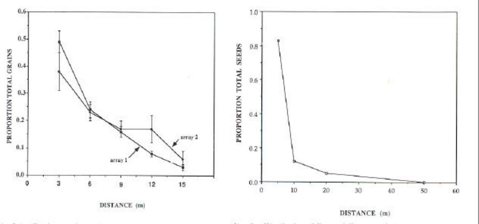
42
Figure A1a. Distributions of dispersal distances of eelgrass (Zostera marina) based on pollen (left graph) and
seed (right graph) dispersal. By combining these distributions, the neighborhood area was estimated
from Na = 4π(σ
2
p
/2 + σ
2
s
), where σ
2
p
and σ
2
s
are the variance in pollen- and seed-dispersal
distributions, respectively. Results from this population indicated that random mating among
individuals occurred on average within a circle of area 524 m
2
(from Ruckelshaus 1996).
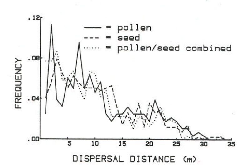
43
Figure A1b. Frequency distributions of pollen, seed and combined pollen and seed dispersal estimated by
identifying and mapping seedlings and parents. Seedlings were assigned to parents based on
genealogy reconstruction using 11 polymorphic enzyme marker loci (from Meagher and Thompson
1987).
44
trend—they would be grouped together in a cluster analysis. Assuming that all else is equal
between the groups would lead to the conclusion that those spawning groups are similar in
abundance over time because they are demographically linked. However, all else is not equal.
For instance, the fish could occur in correlated environmental conditions at any stage of their life
history, a situation that would lead to correlated trends in abundance even in the absence of
demographic connections (Box A1, Hanski and Gilpin 1997, Kendall et al. 2000). Because it is
very difficult to validate such simplifying assumptions, it is better to use multiple, independent
indicators to explore similarities among spawning groups. This method offers more confidence
that groupings are biologically reasonable and that they actually reflect the degree of
reproductive isolation.
Geographic and habitat indicators: A salmon population can be identified, in part, by the
likely spatial distribution of its spawning habitat. Physical features such as a river basin’s
topographical and hydrological characteristics dictate to a large degree where and when salmon
can spawn and delimit the spatial area over which a single group of fish can be expected to
interact. For example, a group of fish returning to spawn in the upper tributaries of a large river
basin such as the Umpqua River on the Oregon coast are not expected to be part of a population
that includes another Oregon coastal river drainage, such as the Alsea River. The long distances
the fish need to travel to spawning habitat in a large river basin combined with generally accurate
homing tendencies make it very unlikely that a single population would encompass multiple
basins or large tributaries.
The geographic characteristics of river mouths and estuaries through which salmon
migrate can also be instrumental in indicating groups of salmon that are likely to be in the same
population. Timing and direction of water flow and spatial distributions of feeding, rearing, and
refuge habitats affect salmonid migratory patterns. For example, the freshwater plume produced
by the Columbia River is a prominent hydrographic feature along the western coasts of Oregon
and Washington. The conditions of the plume vary seasonally; therefore, the timing of the
juvenile salmonid downstream migration affects the salinity, temperature, nutrients, and
sediment load conditions the fish experience in the plume. These conditions, in turn, affect the
likely direction of juvenile fish migrations, their food sources, and their energetic balance.
Geographical and hydrological differences among river drainages imply that ecological
characteristics also differ. For example, some river systems consist of many spring-fed streams,
and others can be made up of streams whose origins are mostly from glacier- or snowmelt-run
off. The productivity, flora, and fauna of glacier- and spring-fed streams are likely to be very
different. Information on freshwater and marine habitat characteristics such as temperature, flow
regimes, prey, pathogens, and predator species can help define the boundaries of salmon
populations. For example, the frequency and types of parasites found in mixed-stock ocean
fisheries have been used to identify salmon populations by determining where the parasite
species occur in freshwater spawning and rearing habitats (Groot and Margolis 1991). In
addition, a population may be identified by examining data on patterns of use of freshwater and
marine feeding, rearing, and spawning habitats; these data are derived from stream surveys,
angler catch, and ocean sampling.

45
Box A1. Assigning “resident” and anadromous salmonids to populations.
One example of the importance of understanding the genetic basis for phenotypic variation when
defining population boundaries is the difficult issue of deciding whether individuals who spend
all of their life history in fresh water (often termed “resident” fish) should be included in the same
population as anadromous fish. This challenge arises in populations of O. mykiss (steelhead and
rainbow trout), O. clarki clarki (coastal cutthroat trout), and O. nerka (sockeye and kokanee) in
many river basins throughout their geographic range (Shapovalov and Taft 1954, Foerster 1968,
Barnhart 1986, Trotter 1989). These distinct life-history forms would be considered to be in the
same population under the following scenarios. First, it could be that the spawning groups of the
two forms are sympatric in time and space—thus allowing interbreeding between the life-history
types. If, in this case, the progeny segregate into alternative life-history forms, it would indicate
that the phenotypic variation occurs in a single population. Assigning fish to a population is
relatively clear in this instance. Alternatively, there could be relatively little inter-breeding
between resident and anadromous salmonids within a stream, but there could be enough lability
in life-history expression that resident parents give rise to a fraction of anadromous offspring each
generation. Those anadromous offspring of resident parents could then interbreed with other
anadromous fish. In this case, whether an individual fish remains in fresh water throughout its
life cycle or migrates to the ocean would be determined largely by environmental conditions.
Under this second scenario, the key information needed to determine whether the different life-
history forms are part of a single population is the degree to which genes are exchanged between
alternative life-history types. Understanding the genetic (as opposed to environmental)
determinants of life-history variation would help in assigning fish with distinct life-history types
to appropriate populations. If the life-history forms are primarily genetically determined and the
forms do not interbreed, fish with distinct life-history types would not be part of the same
population.
There is little empirical evidence supporting either of the above scenarios for any species and, as
expected, the degree to which distinct life-history forms appear to interbreed varies
geographically. It is clear that for all three species there have been periods when the two life-
history forms would have been considered part of the same population; this is because the
“resident” form appears to have arisen multiple times evolutionarily (rev. in Busby et al. 1996,
Gustafson et al. 1997, Johnson et al. 1999). What this means in practice is that it is not possible
to generalize about the extent to which life-history forms within a species are reproductively
isolated. In some cases, selective divergence of the two forms may be maintaining them as
separate populations (e.g., sockeye and kokanee in British Columbia—Wood and Foote 1996). In
other cases, periodic interbreeding during years of high relative abundance of one life-history
form may suggest that they are part of a single interbreeding group (e.g., steelhead and rainbow
trout in the Deschutes River, Oregon—ODFW 1998). The lack of generality is seen in genetic
data for steelhead and “resident” O. mykiss suggesting that in some streams, the two life-history
forms are not distinguishable, but in others, they are genetically distinct (Wilson et al. 1985,
Currens et al. 1987, Leider et al. 1995). Similarly, genetic data for sockeye and kokanee have
shown some groups within a lake system to be genetically similar, and others to be distinct (Foote
et al. 1989, Craig 1995, Taylor et al. 1996).
46
In general, the collective biotic and abiotic characteristics of occupied salmonid habitat
help define a population because we expect that those ecological characteristics constitute the
selective environment in which the salmon exist. If different groups of salmon experience
different selective environments and there is very little migration between those environments,
we expect those groups’ phenotypic characteristics to diverge.
Demographic indicators: To identify a salmonid population, it is necessary to understand the
extent to which it is reproductively isolated from other groups of fish. Demographic
characteristics such as birth and death rates and fecundity determine the population dynamics of
a group of fish. The level of inter-group dispersal influences the degree to which demographic
trajectories are correlated among individual groups, depending on the degree to which the
environmental conditions are correlated. Estimates of adult dispersal in both freshwater and
marine habitats are of critical importance in defining a population unit (see “Evidence for
independent populations,” p. 39).
Long-term abundance data are another type of demographic information that can help
identify a salmon population. Because one of the criteria for defining a population is that it be
largely demographically independent from other groups, abundance data may help show whether
the demographic trajectories of two proposed populations are largely independent of one another.
In cases where the dynamics of two groups of salmon are not correlated with one another, it
might be reasonable to conclude that the two groups are not part of the same population—
provided environmental variation across the range of the groups can be ruled out as a cause of
the uncorrelated dynamics. If the demographics of two groups of salmon do have correlated
dynamics, they might still not be part of the same population. In this latter case, it is possible
that two groups of organisms occur in environments with correlated conditions—resulting in
correlated dynamics between two groups that are not demographically linked (e.g., Grenfell et al.
1998, Kendall and Fox 1998; Fig. A2).
By exploring patterns of abundance among salmonid species within the same geographic
area, it is possible to gather additional information on the degree to which correlated
environmental conditions drive abundance correlations between spawning groups. Assuming
that different species of salmon exhibit different stray rates between spawning sites, any
similarities in population dynamics would most likely be due to similarities in common
environmental conditions the species are experiencing. Therefore, if more than one species
exhibit similar trends in abundance among spawning sites, it would indicate that correlated
environmental conditions are the most likely explanation for abundance correlations among
populations within a species. Teasing apart the effects of correlated environmental conditions
and dispersal to determine the primary cause of population dynamics is a complicated but
important exercise (Kendall and Fox 1998, Kendall et al. 2000).
There are few studies that explore the extent of spatial correlation in salmonid population
dynamics. Rieman and McIntyre (1996) found weak, but statistically significant positive
correlations in bull trout redd counts between streams that were close to one another. The
positive correlations in redd counts were stronger between closer streams, just as one would
expect if the correlated redd counts were due to correlated environmental conditions or dispersal
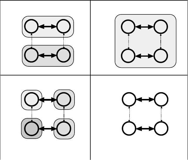
47
a
a
b
b
A.
D.
C.
B.
a
a
b b
a
a
b
b
a
a
b
b
Figure A2. The figure shows why demographic independence is theoretically a useful factor in
designating populations. The circles represent functionally panmictic groups of fish, such as
might be found at a single river reach. (In a panmictic group, all mature individuals are equally
likely to mate with one another.) The arrows represent migration among the breeding groups—
heavy arrows represent high migration rates and the dashed arrows represent low migration rates.
High migration causes demographic coupling among the groups; low migration causes them to
become demographically uncoupled. Breeding groups labeled with the same lower case letter are
considered part of the same population. The different patterned areas represent regions with
different environmental dynamics. As the text illustrates, the simple scenarios depicted in this
figure have important implications for 1) our definition of a population, and 2) how we estimate
the parameters for assessing population status.
Scenario A represents the easiest case to interpret, because the demographic and environmental
processes have the same boundaries. The two groups labeled “a” are part of the same population
because the high rate of migration between them means that any extinction of a single group
would only be temporary because the remaining group could recolonize the other—thus rescuing
it from extinction. The “a” groups and “b” groups are not considered to form a single population
because there are not enough migrants from “b” to prevent the “a” population from going extinct,
and vice versa. Because population and environmental boundaries coincide in this scenario,
demographic processes and environmental forcing will work in concert to create similar
abundance fluctuations in all the groups within a population and independent abundance
fluctuations among different populations.
In contrast, both populations in scenario B share the same environmental dynamic. If
environmental forcing were strong (i.e., abundance is strongly influenced by varying
environmental conditions), then fish abundance would vary in a similar fashion in each
population. However, “a” and “b” would still be considered independent populations because the
risk of extinction due to demographic processes in “a” is independent of the risk in “b.”
48
In scenario C, all four groups experience different environmental dynamics, and if environmental
forcing were strong, the abundance variation would be independent for all four groups. However,
“a” is still a legitimate population because of the high inter-group migration rate. Thus for the
“a” groups, individual reaches within a single population may temporarily go “extinct,” but when
the population is considered as a whole, as long as a single reach remains extant, the population
will survive. These types of substructured populations are discussed in detail in “Spatial
Structure,” p. 18.
In scenario D, we show groups of fish in a hypothetically constant environment. In a constant
environment, abundance changes would be driven completely by demographic and genetic
processes. Even if they were to start with the same population size, the abundance patterns for
population “a” would deviate from the abundance pattern of population “b.” Our definition
focuses on the extinction risk that independent populations face. As a consequence, separate
populations could abstractly be described as being sufficiently isolated, but in a constant
environment they would have largely uncorrelated demographic trajectories.
49
among nearby spawning areas. Milner et al. (1993) explored correlations in salmonid densities
between sites within and between tributaries in a river in North Wales. Atlantic salmon and
brown trout fry and parr densities were compared at several sites within each of three tributaries
to the River Conwy. For both trout and salmon, weakly significant positive density correlations
were found both within and between the tributaries, though the variance synchrony was stronger
within tributaries than it was at larger spatial scales (Milner et al. 1993). McKinnell (1999)
reported on synchronized freshwater catch and recruitment dynamics for Atlantic salmon in
Swedish rivers. And, like the other studies, he found a weak relationship between the survival of
salmon from different hatcheries and the distance between them. Fish from hatcheries that were
closer together were slightly more correlated in terms of marine survival than were fish from
hatcheries that were separated by greater distances (McKinnell 1999). Bradford (1999) found
positive covariation in coho smolt abundance for streams in Western North America that were
separated by distances less than 20-30 km. In summary, the evidence for spatial correlation in
salmonid population numbers suggests that abundance variations among fish in streams that are
closer to one another tend to be significantly positively correlated, but the correlations are often
not very strong.
Genetic indicators: Genetic characteristics are useful in identifying salmon populations because
they indicate the extent of reproductive isolation among groups. Molecular genetic markers such
as allozymes and nuclear or mitochondrial DNA markers can be used to statistically describe an
organism’s population structure based on their genetic similarities. In addition, studies of
quantitative trait variation (e.g., life-history characteristics) can often help to distinguish
salmonid groups. Salmon populations, stocks, and ESUs have been identified with the help of
genetic markers and life-history traits (WDF et al. 1993, ODFW 1995, Weitkamp et al. 1995,
Busby et al. 1996, Myers et al. 1998, Johnson et al. 1999). The spatial distribution of particular
alleles and their frequencies can also be used to define the spatial scale(s) over which groups of
salmon are structured. The nature of genetic data allows for a hierarchical exploration of the
geographic structuring of salmon populations. Nevertheless, just as it is difficult to use
geographic and abundance indicators to identify populations, the extent to which genetic markers
can be used to identify independent populations still needs to be determined. Translating the
genetic structure of a salmonid species into a set of independent populations is not a simple task,
because of the assumptions about population structure that must be made when estimating allele
frequencies. As with other indicators of spatial structure, it is necessary to estimate the
significance of the genetic structure in terms of population and extinction dynamics in order to
identify populations.
For the most part, genetic markers are straightforward indicators of genetic variation
among groups. However, there are some instances where genetic data can be uninformative or
misleading (Whitlock and McCauley 1999). For example, if there is insufficient variability at
marker loci or only a small number of marker loci are used, genetic markers may indicate little or
no population structure when it is in fact present. In addition, using molecular genetic markers to
estimate degree of reproductive isolation may require certain assumptions (e.g., that the groups
of organisms sampled are in drift-migration equilibrium). As discussed elsewhere (see
“Diversity,” p. 19), salmon populations are dynamic in space and time, and in many cases their
evolutionary dynamics are not likely to be at equilibrium. For example, a subpopulation founded
by a few individuals during a colonization event is likely to diverge genetically from the
50
founders’ original subpopulation because of the genetic drift that occurs during the sampling
from the parent subpopulation. This would be true even if, over the course of many generations,
the two subpopulations were connected by high enough levels of migration to be considered part
of the same population. Because extinction and recolonization processes are thought to occur
relatively frequently in some salmon species in some locations (Mangel and Tier 1994, Dunham
and Rieman 1999), it is not a simple matter to attribute causes (e.g., low levels of gene flow vs.
recent founding event) to observed population structure. This may also present a problem when
attempting to identify populations that have experienced chronic declines in abundance, if, for
example, a previously contiguous population has become fragmented into what now appear to be
several isolated populations. Rigorous modeling or empirical comparisons to patterns of genetic
variation in healthier systems may help overcome some of these potential problems (Currens et
al. 1996). Finally, although salmon populations are likely to be commonly perturbed from
equilibrium conditions, theoretical work has shown that under some circumstances estimates of
inter-population gene flow obtained from population structure statistics approach their
equilibrium values fairly rapidly (Slatkin and Barton 1989, Slatkin 1993, Crow and Aoki 1984).
Recently developed likelihood methods for estimating gene flow and divergence time may
provide more accurate estimates of gene flow than F
ST
based estimates, especially in non-
equilibrium situations (e.g., Nielsen and Slatkin 2000).
It is appealing to use molecular genetic markers to survey and identify salmon
populations because of the large sample sizes that can be obtained with relatively little effort.
Variation in genetically-based life-history traits can also be used to help determine population
boundaries. However, gaining an understanding of the distribution of genetically-based life
history and other quantitative traits is much more labor-intensive and, as a result, this
information is usually lacking for most natural populations. In practice, phenotypic variation in
traits such as run timing, size at migration, and ocean and estuarine migratory patterns has been
used to help delineate salmonid groups. This approach is probably most useful at relatively large
geographic scales—such as ESUs (e.g., Busby et al. 1996, Myers et al. 1998)—because the
potentially confounding effects of environmentally-induced phenotypes are less likely to occur
over large geographic regions. Technically, only those phenotypic traits based on underlying
genetic variation (rather than environmentally-induced variation) can help define a population
because populations are defined on the basis of reproductive isolation and, ultimately,
demographic independence (see Figure A2). However, in combination with other population
indicators, spatially-structured phenotypic variation within an ESU could be used as a proxy for
genetically-based variation.
Rigorous, direct methods for estimating the genetic components of quantitative trait
variation involve controlled breeding designs and rearing offspring to life stages that express
quantitative traits of interest (Falconer and Mackay 1996). Because of the relatively long
generation times for Pacific salmonids, there are many challenges associated with rearing
offspring from controlled matings. Indirect evidence for the extent of genetic (vs.
environmental) sources of variation in phenotypic traits can be obtained from studies of traits
within maternal or paternal families, an approach that is somewhat easier to use for salmon,
especially in hatchery populations (Silverstein and Hershberger 1992, Beacham and Evelyn
1992, Heath et al. 1994, Herbert et al. 1998, Mousseau et al. 1998, Hard et al. in press). A few
studies of quantitative trait variation in salmon have been conducted and they have found that a
51
significant portion of the observed phenotypic variation in some life-history and meristic traits is
genetically based (see “Diversity,” p. 19). Such results suggest that describing the spatial
distribution of life-history variation (and other quantitative traits) for salmon may be a good
indicator of population structure, even if the actual genetic basis for trait variation is not known
in most cases.
In a comparative review, Healy and Prince (1995) showed that in general, phenotypic
variation among salmon populations is much greater than allozyme frequency variation.
Molecular markers are ultimately a better tool for grouping fish than phenotypic variation for at
least two reasons. First, selection is expected to be greater on quantitative traits than on
molecular loci (which are presumed to be neutral). Estimating reproductive isolation from
divergence of selected characters requires making a number of restrictive assumptions that are
not needed when using neutral markers (Hartl and Clark 1989). Second, some portion of
phenotypic variance is due to environmental variation and is therefore of no use in estimating
reproductive isolation among groups (Falconer 1981). Nevertheless, where it is difficult to
obtain useful data, a useful proxy (e.g., phenotypic variation) is better than no information at all.
The paucity of information on quantitative trait variation among salmon populations has
unfortunate consequences in terms of our ability to evaluate population and ESU viability. This
is partly because such variation is a good indicator of the extent and nature of a population’s
local adaptations. The degree to which a population exhibits local adaptation is an important
indicator of its response to environmental changes and, ultimately, the probability of its
persistence. More generally, it is useful to know the distribution of locally adapted traits among
groups of salmon in order to describe diversity patterns at a number of spatial scales. As
“Diversity” (p. 19) discusses, genetic diversity is a critical factor in long-term persistence at the
population, ESU, and species levels. It also is an important descriptor of the biological
components of the evolutionary lineages that are the focal points for conservation.
Identifying populations—combining the evidence
Without evidence of independent population dynamics or extinction probabilities,
identifying populations involves combining stray rate estimates with any information on
indicators of population structure discussed previously. Ford et al. (2000) summarizes methods
for identifying populations using available data for spring-run chinook salmon and steelhead in
the upper Columbia River, Washington, region.
Existing Approaches to Identifying Salmon Populations or Groups
States and other groups that manage salmon have, for management purposes, employed a
number of different definitions for particular groups of fish and many of those definitions are
similar to the population definition we propose in this document. The Washington Department
of Fish and Wildlife (WDFW 1998) defines a stock using Ricker’s (1972) definition; although
they do acknowledge that smaller production units may be important and that considerable
uncertainty arises when this definition is applied to groups of salmon (WDFW 1998). In
practice, salmon stock boundaries have been identified using information on such aspects as run
52
timing, size and age at migration, ocean migration patterns, spawning locations, and genetic
similarities. For the purposes of reporting the status of coastal cutthroat trout, the WDFW
introduced the concept of a stock complex, or a “group of stocks typically located within a single
watershed or other relatively limited geographic area” (WDFW 1998). The WDFW found that
identifying individual stocks of coastal cutthroat trout was more challenging than identifying
salmon and steelhead stocks. This was due, in part, to the wide range of migratory behaviors that
cutthroat trout exhibit and because there is a great deal of uncertainty about the genetic
relationships among different life-history forms (WDFW 1998). The WDFW also uses various
genetic, geographic, and life-history data to delineate Genetic Diversity Units (GDUs), and
Major Ancestral Lineages (MALs), both of which attempt to define conservation or management
units at taxonomic levels higher than populations but lower than species. For example, the
WDFW defines an “Upper Columbia Summer + Fall, Snake Fall and Mid- and Lower-Columbia
Chinook” Major Ancestral Lineage within which there are 7 Gene Diversity Units (Marshall et
al. 1995). Three of these GDUs are contained within the Lower Columbia River chinook salmon
ESU (Myers et al. 1998). In other cases, such as Puget Sound chinook salmon, the MAL and the
ESU boundaries are equivalent (Marshall et al. 1995, Myers et al. 1998).
Along similar lines, the Oregon Department of Fish and Wildlife (ODFW) also uses a
definition of “population” similar to Ricker's (1972) definition. They identify Gene
Conservation Groups (GCGs), which are defined as genetically distinct clusters of one or more
populations within a taxonomic species that arise when gene flow between the cluster and other
populations of the same species is zero (or very low) over a sufficiently long period of time
Kostow et al. 1995, OAR 635-07-501). The GCGs are identified using molecular genetic and
geographic information to define groups of spawning populations that have similar genetic and
life-history traits (Kostow et al. 1995). The ODFW often uses genetic data to delineate GCG
boundaries, but if such data are not available, geographic proximity is used as a guide in
identifying groups (Kostow et al. 1995).
Although the WDFW/tribal and the ODFW’s population definitions are based on the
same Ricker stock definition, in practice, the agencies tend to reach different conclusions as to
what constitutes a “population.” The WDFW and tribal (SASSI) stocks (WDF et al. 1993)
generally encompass larger geographic areas than what the ODFW would consider a population
(Kostow et al. 1995). Part of this difference may result from geographic differences between
two states. Nevertheless, a large part of the difference is likely due to different interpretations of
the “substantial degree do not interbreed” portion of Ricker’s definition. By adding independent
population dynamics and extinction risk to Ricker’s definition, we are attempting to arrive at the
clearest possible interpretation of the word “substantial.”
The Pacific Fishery Management Council's Pacific Coast Salmon Fishery Management
Plan recognizes numerous “stocks” of chinook and coho salmon for purposes of ocean harvest
management. The plan has no specific criteria for designating stocks, but in general they cover
larger areas than do the populations defined here. The proposed draft Amendment 14 to the plan
restructures the management stocks slightly to provide more comprehensive coverage of the
ESUs defined in NMFS' ESA listings, but retains the larger geographic scale of the present plan
(PFMC 1999). We expect that each PFMC stock would be made up of one or more populations
as they are defined here.
53
The state of California delineates separate runs of salmonids based on genetic distinctness
and life-history differences such as spatial and temporal variation in run timing and juvenile
outmigration (CDFG 1998). They manage these distinct runs (e.g., Central Valley spring vs. fall
chinook salmon) separately from one another in setting harvest levels and escapement goals.
Their “runs” would probably be composed of several populations as we have defined them in
this document. In addition, Barnhart (1994) has used geographic distribution, life history,
straying, and genetic data to identify populations and meta-populations of several salmonid
species in the Klamath-Trinity Basin of California.
Population Size
Introduction
Small populations face a host of risks intrinsic to their low abundance; conversely, large
populations exhibit a greater degree of resilience. A large part of the conservation science
literature is directed toward understanding and predicting the effects of population size (Soulé
1986, 1987, Meffe and Carroll 1994, Caughley and Gunn 1996). Population abundance is an
important determinant of risk, both by itself and in relationship to other factors. There are a
variety of risks associated with the demographics of small populations, including both directional
and random effects. Directional effects include two forms of population density-dependence:
compensation and depensation. Random effects on population dynamics include demographic
stochasticity, environmental stochasticity, and catastrophes (Gilpin 1987, Lande 1993). (Note
that only demographic and local environmental stochasticity are considered at the population
level here; large-scale environmental effects and catastrophes are considered at the ESU level,
see “Viable ESUs,” p. 125.) Lande (1993) used a simple population dynamics model to examine
the relative risks associated with these three effects as a function of carrying capacity and long-
run population growth rate. He concluded that, for populations with a positive long-run average
growth rate, risks from demographic stochasticity are substantial only at very low population
sizes, while environmental stochasticity and catastrophes are the dominant risks at higher
population sizes. For populations with negative average growth rate, risks from all three types of
variation change nearly exponentially with capacity, and thus all may be important.
Small populations also lose adaptive variation and gain maladaptive variation at higher
rates than large populations (Mills and Smouse 1994, Lande 1995, Schultz and Lynch 1997),
both phenomena generate lower average fitness and a higher probability of extinction. Finally, if
populations are declining due to deterministic effects (e.g., habitat degradation or overharvest),
population abundance combined with measures of trends and productivity can be an indicator of
how long it will take the population to reach a critically low abundance level (Caughley 1994).
Given these considerations, it is clear that risk tends to vary inversely with abundance if
other factors are held constant. This means we can, in theory, define simple numeric thresholds
to delineate different risk categories ranging from healthy down to extinct. In the following
discussion, we focus on two such thresholds: 1 ) a Aviability@ threshold above which populations
54
have negligible risk of extinction due to local factors, and 2) a Acritical@ threshold below which
populations are at relatively high risk of extinction in the near future. However, putting numbers
on such thresholds is a difficult task for three reasons. First, other factors are not constant and
often correlate with abundance levels; this means a pure abundance threshold must be
conditional on particular conditions, especially those relating to population trend and variability.
Second, the theory relating abundance to extinction risk is based on relatively simple models of
population dynamics, and it is not clear how to relate this theory to the complexities of real
populations. Third, our ability to accurately measure population abundance and density is quite
limited, so there is a great deal of estimation error in any analysis of abundance or risk. For all
these reasons, there is a great deal of uncertainty associated with any thresholds that may be
established.
All else being equal, small populations are at greater risk of extinction than large
populations primarily because several processes that affect population dynamics operate
differently in small populations than in large populations. These are: deterministic density
effects, environmental variation, genetic processes, demographic stochasticity, ecological
feedback, and catastrophes. The first five of these processes are discussed in more detail.
Catastrophes (environmental events that severely reduce population abundance in a relatively
short amount of time) affect more than one population over a large geographic area, so the
effects of catastrophes are considered in the section on ESU-level viability (“Viable ESUs,” p.
125) rather than here.
Density effects
Population ecologists typically divide processes that affect birth and/or death rates into
two types: density-dependent effects, and density-independent effects (for example, Nicholson,
1933, Wilson and Bossert 1971, Ricklefs 1973, Hilborn and Walters 1992). Because of the
structure of the differential-equation models that describe these different effects, density-
independent effects are often termed “linear” effects, while density-dependent effects are termed
Anon-linear@. Density-dependent effects on population productivity arise from two competing
processes: compensation (a decrease in productivity with increasing density) and depensation (an
increase in productivity with increasing density). Compensation is a stabilizing influence. With
it, an increase in population is offset by a subsequent decline in productivity; it is most important
at higher abundance levels. Depensation is a destabilizing influence and is important mainly at
very low abundance levels.
Figure A3 illustrates the typical shape of curves relating parental density to offspring
density for deterministic populations with positive intrinsic growth rate exhibiting no density-
dependence, compensation only, and compensation plus depensation. In this illustration, it is
clear that the population with linear dynamics will increase in each generation regardless of
abundance and that the population with compensation only will reach a stable equilibrium at a
positive abundance where the curve crosses the replacement line. The population with both
compensation and depensation has three equilibrium points (points where it crosses the
replacement line): stable equilibria at zero (extinction), high abundance, and an unstable
equilibrium at intermediate abundance. If population abundance is above the unstable
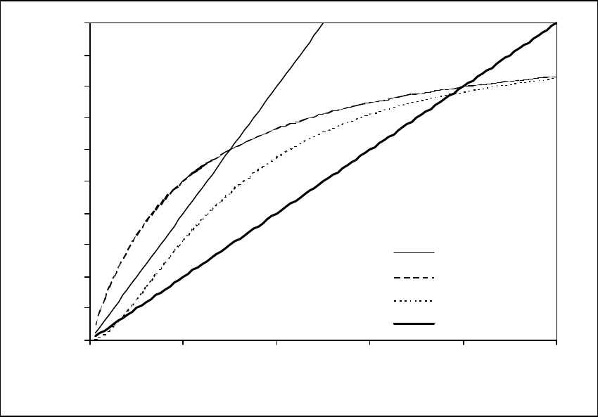
55
0
100
200
300
400
500
600
700
800
900
1000
0 200 400 600 800 1000
Parental Abundance
Offspring Abundance
Linear
Compensation
Depensation
Replacement
Figure A3. Typical shape of parent-offspring (or stock-recruit) curves for populations with no density-
dependence (“Linear”), compensation only, and compensation plus depensation. The
replacement line (where offspring equal parents) is included for reference.
56
equilibrium, the population will more than replace itself and move toward the upper stable point;
if it is below the unstable point, it will fail to replace itself and move toward zero.
Compensation at high abundance occurs because there is increasing competition for limited
resources as a population expands to fill (or exceed) available habitat. Compensation=s negative
relationship between productivity and abundance can give a population substantial resiliency
because any decline in abundance is offset by an increase in productivity that will tend to restore
the population to some equilibrium level. The role of compensation is widely recognized in
fishery management through the use of compensatory production models, usually following the
form of Ricker or Beverton-Holt recruitment models (Ricker 1975, Hilborn and Walters 1992).
For salmon, there is extensive literature discussing models and evidence for compensatory
processes in salmon (for example, Ricker 1954, Skud 1973, Solomon 1985, Peterman 1987).
In contrast, when abundance is very low, depensation will accelerate declines and slow
recovery. Depensatory processes at low population abundance (also termed “allele effects” or
“inverse density dependence”) will result in high extinction risks for very small populations
because any decline in abundance further reduces a population=s average productivity, resulting
in a spiraling slide toward extinction. A variety of processes can lead to depensatory population
behavior, and such effects are documented for a wide variety of organisms (reviewed by
Courchamp et al. 1999). The most commonly cited of these are the uncertainty that mates will
be able to find one another in sparse populations (Dennis 1989), randomly skewed sex ratios at
low abundance (Gabriel and Bürger 1992), non-linear response of predators to shifting prey
abundance (Peterman 1987), and scaling effects of random variation among individuals (Lande
1998). Synergistic interactions among these effects may also increase risks at low abundance
(Stephens and Sutherland 1999). Fundamental population theory clearly requires that
depensation become significant at some low abundance level in all populations, but the exact
level where this occurs, and whether depensation will overcome compensation, depends on the
behavior and ecology of individual populations. For example, population density must be high
enough to provide sufficient temporal and spatial overlap for males and females to find each
other to spawn, but the level of population abundance necessary for this to occur depends on the
life-history characteristics of the population in question as well as aspects of the population=s
habitat. In consequence, populations that return to spawn over long periods of time or inhabit
large geographic areas may need to be more abundant to be considered viable than those with
more limited spatial or temporal spawning distributions.
In contrast to compensation, fish population models rarely include depensation, although
that situation is changing (Ludwig 1998). The direct evidence for depensation in salmonid
populations is mixed. Peterman (1987) summarized evidence from a few studies indicating
depensatory predation mortality among juvenile salmon, and used a simple population model to
show that such mortality could explain observed population dynamics. In contrast, Myers et al.
(1995) found significant evidence of depensation in population data for only 2 of 11 populations
of salmon examined. Liermann and Hilborn (1997) found only one salmon population out of 27
that clearly exhibited depensation; it was uncertain whether depensation was evident in the
remaining 26. Because of the great uncertainty surrounding depensation parameter distributions
in their study and the consequences of ignoring depensation if it really is significant, Liermann
and Hilborn recommended that fishery analyses employ models that incorporate depensation.
57
Translating these effects into specific criteria for “viable” or “critical” abundance levels
is no simple task. The specific form and function of both compensatory and depensatory
processes depend on species- and population-specific life-history characteristics that are difficult
to measure accurately. Both types of effect may vary either abruptly or smoothly with changing
abundance (for example, Getz and Haight 1989, Dennis 1989), and either pattern could cause
abrupt thresholds in population dynamics. When these deterministic effects are combined with
stochastic effects, the situation becomes even more intractable. However, some general
guidance can be noted. First, it is obvious that a population that is unable to replace itself is in
trouble, so we can say that a population is in critical condition when it is so low that depensatory
processes are expected to reduce average production below replacement. Similarly, we can say
that a population that is near its compensatory stable equilibrium abundance is likely to be safe
from deterministic extinction risks; however, such a level may be well above the actual lower
threshold of viability as we have defined that term.
Precisely estimating critical population levels based on these principles is impossible
without extensive observations of population dynamics across a wide range of abundances;
however, a number of approaches can be used to provide reasonable estimates of such levels.
Estimates of habitat capacity can be used to define a likely range for compensatory processes.
Similarly, theory can be used to establish upper and lower limits for depensatory processes based
on mate-finding, predator-prey interactions, sex-ratio stochasticity, etc.
Environmental variation
Environmental variation can cause small populations to go extinct when chance events
frequently reduce survival or fecundity to low levels over an extended time. There is an
extensive amount of literature on the relationships among extinction risk, persistence time,
population abundance and level of variation in demographic parameters (for example,
MacArthur and Wilson 1967, Tuljapurkar and Orzack 1980, Goodman 1987, Belovsky 1987,
Lande and Orzack 1988, Thomas 1990, Dennis et al. 1991, Lande 1993).
One obvious conclusion from this literature is that there are no simple, generic abundance
levels that can be identified as viable; the form of the population model used (e.g., linear or non-
linear, simple or age-structured), average parameter values, and degree of environmental
variation all combine with abundance to determine extinction risk. In general, model results
suggest that numbers greater than 1,000 to 10,000 are often needed to protect a population from
moderate-to-high levels of environmental variation (Belovsky 1987, Goodman 1987, Thomas
1990). Thomas (1990) examined both empirical evidence and model results to determine “safe”
(i.e., low extinction risk) abundance levels. Thomas concluded that Asafe@ levels vary depending
on the degree of natural variation in population abundance. However, Thomas did provide
guidance regarding appropriate population abundance (geometric mean abundance per
generation) for general classes of organisms, suggesting that 1,000 is adequate for species of low
variability, and 10,000 is usually adequate for the most variable bird and mammal species. For
extremely variable species, such as many insects and the most variable of vertebrates, Thomas
recommended increasing these values by an order of magnitude. Salmon have relatively high
fecundity (thousands of eggs per female), and therefore have the potential for rapid changes in
population abundance. However, unlike insects, salmonids exhibit age-structure and overlapping
generations that may reduce the variability of adult populations. Thus, salmonids are probably at
58
the high end of the variability spectrum for typical vertebrate populations. Thomas= guidance
might therefore translate to a recommended Asafe@ population abundance of somewhere between
1,000 and 10,000 spawners per generation, depending on the degree of variability in abundance
of a given population. Thomas= approach is difficult to apply in practice, because it assumes:
1) a complete census of all individuals in a generation, 2) a population that is stable about some
mean value (i.e., no upward or downward trend), and 3) that there are no density-dependent
effects. In 1995, NMFS considered using this method to set recovery abundance goals for Snake
River salmon populations (NMFS 1995b), but found there was not enough data to categorize
populations into Thomas= variability categories except for a number of spring/summer chinook
salmon stocks; these stocks exhibited relatively low variability during a thirteen-year period.
From this, and considering that the period for which there were data was one of relatively stable
environmental conditions, NMFS concluded that variability for these populations was probably
low to moderate and thus that safe abundance levels would fall between 1,000 and 5,500
spawners per generation. Considering that spring-summer chinook exhibit a 4- or 5-year mean
generation time, these 1,000 to 5,500 spawners per generation would translate to 200-250 to
1,100-1,375 spawners per year.
Genetic processes
There is a great deal of theoretical work relating population size to genetic diversity and
the degree of inbreeding within populations (e.g., Wright 1938, Crow and Kimura 1970). There
is also a body of theoretical work on the relationship between population size and the
accumulation of deleterious alleles and how this affects population viability (Lynch 1990, Lande
1994, 1995, Schultz and Lynch 1997), and on the relationship between the amount of genetic
diversity in a population and the population's fitness (e.g., Burger and Lynch 1995). Many of the
classical population genetic models that have been used to explore the relationships between
population size and level of inbreeding or genetic drift do not accurately correspond to typical
salmon life-histories (i.e., semelparous overlapping generations). Waples and Teel (1990) and
Waples (1990a, 1990b) have updated some of these models to take into account typical salmon
life-history patterns. One aspect of salmon biology that has not received a great deal of attention
in population viability models is the fact that salmonids are partially tetraploid (reviewed by
Allendorf and Thorgaard 1984). Partial tetraploidy may reduce the severity of inbreeding
depression in comparison to the amount seen in diploid organisms because, all else being equal,
tetraploids are less homozygous than diploids. However, inbreeding depression has been
observed in Pacific salmonids, so the benefits of tetraploidy might not be substantial.
One important concept from population genetic theory is that of effective population size
(N
e
, Wright 1931, Crow and Kimura 1970). The effective size of a population is defined as the
size of an idealized population that would produce the same level of inbreeding or neutral
variance in allele frequency (genetic drift) seen in an observed population in which one is
interested (see Hartl and Clark 1989, Caballero 1994 for reviews). Attributes of such an
idealized population typically include discrete generations, equal sex ratios, binomial variance of
reproductive success, random mating, constant breeding, population size, and non-selective
gamete-to-adult mortality. Violating any of these attributes usually increases the rate of
inbreeding or drift in comparison to the idealized case, and therefore reduces effective size of the
population of interest. Effective size can be defined with respect to either inbreeding or genetic
59
drift, as well as other population attributes (reviewed by Crow and Kimura 1970). For example,
the inbreeding effective size refers to the size of an ideal population that would produce the same
rate of inbreeding as an observed population. The variance effective size refers to the size of an
ideal population that produces the same rate of allele frequency change due to genetic drift as an
observed population. The inbreeding and variance effective sizes are usually nearly identical
when populations are of constant size, but they generally differ when populations are growing or
shrinking (e.g., Crow and Kimura 1970, Ryman et al. 1995). Because almost no natural
populations are “ideal,” the effective size of a population is almost always smaller than the
observed number of breeding individuals (reviewed by Frankham 1995). Effective size is a
useful concept because it is a parameter that can be estimated from real populations, and
therefore, acts as a bridge between the complexities of real populations and the necessarily
simplified assumptions made in population genetic models. The effective size of a population
generally refers to the population size of an entire generation, whereas the effective number of
breeders (N
b
) refers to the effective number of individuals in a single year (Waples and Teel
1990, Waples 1990a). For species or populations with multiple overlapping age classes (i.e., all
the Pacific salmon species expect for pink salmon and perhaps some coho salmon populations),
the effective population size per generation is approximately equal to the geometric mean of the
effective number of breeders per year multiplied by the number of years in a generation (itself
approximately equal to the mean age at reproduction). For example, a population with a four-
year generation time and a geometric mean N
b
of 100/year would have a N
e
of ~400/generation
(Waples 1990b).
Several examples from fruit flies (reviewed by Wright 1977) and Tribolium (Rich et al.
1979) in laboratory settings give empirical evidence of the relationship between population size
and the rate of loss of genetic diversity. In natural populations, there are several examples of low
levels of genetic diversity associated with known severe bottlenecks; these include elephant seals
(Lehman et al. 1993), prairie chickens (Bouzat et al. 1998a, b), and koalas (Houlden et al. 1996).
Quinn et al. (1996) found lower levels of protein and DNA heterozygosity in New Zealand
chinook salmon than in the Californian founder population, a result consistent with a known
founder effect. Waples and Teel (1990) discuss year-to-year changes in protein allele
frequencies in Oregon hatcheries that they attributed to genetic drift due to small broodstock
sizes. In a literature survey of genetic variation in many species, Nei and Graur (1984) found a
small but statistically significant correlation between the level of protein heterozygosity and
species-wide abundance. Latter et al. (1995) measured the rate of inbreeding at small effective
populations sizes in Drosophila and found that inbreeding as measured by homozygosity at
specific marker loci increased somewhat more slowly than predicted by theory, although
substantial inbreeding depression was still observed.
The empirical evidence to date points to a complicated relationship between levels of
genetic diversity (as measured by protein or DNA heterozygosity) and population fitness or
viability. O'Brien et al. (1983, 1985) suggested that very low levels of heterozygosity in the
South African cheetah were correlated with poor fitness (low sperm counts, susceptibility to
disease), but other authors have disputed these conclusions (e.g., Pimm 1991). In the case of the
prairie chickens cited, a population that experienced a severe reduction in abundance was less fit
than two other populations that maintained large population sizes (Bouzat et al. 1998a, b). Leary
et al. (1983, 1985a, b) found a correlation between bilateral asymmetry and level of protein
heterozygosity in rainbow trout and several studies have found correlations between protein
60
heterozygosity and fitness in marine invertebrates (e.g., Koehn et al. 1988). Saccheri et al.
(1998) found a significant correlation between extinction and level of protein heterozygosity
(itself correlated with inbreeding level in this study) in natural populations of butterflies in
Finland. Quattro and Vrijenhoek (1989) found a significant correlation between protein
heterozygosity and fitness in a Sonoran topminnow. Frankham (1995) summarized studies of
genetic variation in a large number of endangered species and found lower than average levels of
genetic variation in most of them. The predominance of sexual species and the relative rarity of
old asexual lineages also argue for the general importance of genetic variation to animal
populations (reviewed by Judson and Normark 1996). Although these and other studies certainly
suggest that there is relationship between genetic diversity and population fitness across a wide
variety of organisms, there are notable examples where a lack of genetic diversity has not
stopped a population from persisting or growing, at least in the short term. In the case of the
elephant seal cited, for example, the species has recovered from about 100 individuals in the late
1800's to 125,000 in 1989 (discussed in Caughley and Gunn 1996) despite its near lack of
measurable genetic diversity. E.H. Bryant and co-authors have published a series of papers on
the quantitative genetic effects of repeated bottlenecks in populations of houseflies and found
that additive genetic variation in the morphological traits they measured generally was not
reduced by even very severe bottlenecks (e.g., Bryant and Meffert 1990). Finally, in many cases
it is difficult to untangle the effects of genetic diversity on population fitness from the effects of
inbreeding on population fitness, because genetic diversity and inbreeding are often correlated.
A reduction in fitness associated with inbreeding (inbreeding depression) has been
demonstrated for a wide variety of organisms in captivity (reviewed by Wright 1977, Thornhill
1993, Falconer and Mackay 1996, Lynch and Walsh 1998); these include rainbow trout and
Atlantic salmon (reviewed by Tave 1993). Further examples of an association between
inbreeding and a reduction in fitness or extinction in natural habitats include the evening
primrose Clarkia pulchella (Newman and Pilson 1997), white-footed mice (Jimenez et al. 1994),
and Finnish butterflies (Saccheri et al. 1998) and Sonoran topminnows (Quattro and Vrijenhoek
1989). Frankham (1998) estimated inbreeding coefficients in 210 populations found on islands
and concluded that inbreeding depression was sufficiently high to be a contributing factor in the
higher rates of extinction that island populations experience in comparison to mainland
populations. Several studies have shown that the rate of inbreeding (as opposed to the final level
achieved) has an effect on inbreeding depression. For example, Latter et al. (1995) and Latter
(1998) found that when Drosophila were inbred at a slow rate (~1%/generation), the resulting
inbreeding depression was less than the level of depression observed in other studies where the
rate of inbreeding was higher. About 25% of the populations that inbred at this slow rate
nevertheless went extinct due to genetic causes within a period of 200 generations.
The conservation literature contains a number of recommendations on guidelines for the
minimum population sizes needed to avoid deleterious genetic effects. All of these
recommendations are based on effective number of breeders per generation and for a number of
reasons must only be considered as rough guidelines. In order to avoid inbreeding depression,
Franklin (1980) suggested, based on empirical data from animal breeding studies, that an
effective size of 50 was reasonable. Franklin (1980) and Soulé (1980) suggested that an
effective population size of 500 is necessary to retain sufficient genetic variation for long-term
population persistence. This value is based on estimates of the rates at which variation in an
isolated population is added by mutations, and removed by drift and selection. Recently Lande
61
(1995) has pointed out that because ~90% of new mutations are unconditionally deleterious (and
therefore do not contribute to future evolution), a more realistic long-term minimum viable
effective population size may be closer to 5,000 per generation. Using similar arguments, Lynch
(1996) has suggested that an effective size of ~1,000 is usually large enough for a population to
maintain genetic variation. Based on the probability of losing rare alleles, Waples (1990a) has
suggested that 100 effective breeders/year is necessary to maintain genetic variation in salmon
populations in the short-term. These general recommendations have some limitations that must
be understood before they are used to help determine levels of abundance necessary for viable
salmonid populations. First, they are based on models of single, reproductively isolated
populations. As the term is used in this document, a population is substantially reproductively
isolated, but may receive low levels of gene flow from other populations. Gene flow, like
mutation, is a source of genetic variation, so it is likely that populations connected by gene flow
will have somewhat smaller minimum genetically viable population sizes than completely
isolated populations. Second, the genetic parameters that form the basis for the Franklin (1980)
and Lande (1995) recommendations were estimated from data obtained from only one species
(Drosophila melanogaster), and must therefore be regarded as preliminary. Nonetheless, these
recommendations may be reasonable as starting points for determining the minimum abundance
necessary for long-term genetic viability, especially in the absence of additional information.
In order to convert these recommendations of effective population size per generation to
salmon spawning abundance per year, it is necessary to know the ratio of the effective number of
breeders to the observed number of breeders (N
b
/N ratio) and the generation time for the
population in question. Several studies suggest that a N
b
/N ratio of 0.3 is approximately correct
for salmon and steelhead in general (see following AAssessment Methods@). With this ratio, the
recommended minimum long-term genetically viable population sizes discussed above range
from 1,670/generation (Franklin 1980 and Soulé 1980) to 16,700/generation (Lande 1995). The
minimum spawning size recommended by WDFW (1997) falls in this range (3,000/generation).
For populations that spawn at multiple age classes, the spawners/generation value must be
divided by the generation length (median age of reproduction) to obtain the corresponding
numbers of spawners per year. For example, many chinook salmon populations have about a
four-year generation time (reviewed by Healey 1991). A range of ~417 to ~4,170 breeders per
year, therefore, may be reasonable minimum values for maintaining sufficient genetic diversity
to ensure long-term persistence of chinook salmon populations. Based on genetic evidence,
Allendorf et al. (1997) concluded that salmon populations with N
e
below 500 (or N below 2,500)
per generation would be at high risk and populations with N
e
below 50 (or N below 250) per
generation would be at very high risk. Wainwright and Waples (1998) noted that if demographic
factors were included, thresholds for these categories would be higher, but they did not suggest
specific values.
Demographic stochasticity
Demographic stochasticity refers to the effects of apparently random events associated
with mate choice, fecundity, fertility, and sex ratio and tend to cause higher extinction risks in
small populations than in large ones. Mathematical theory for extinction due to random variation
in birth and death rates among individuals in a population was first developed in the 1930s (see
Goodman 1987, Gabriel and Bürger 1992), but was first widely applied in developing island
biogeography theory (MacArthur and Wilson 1967, Richter-Dyn and Goel 1972). The
62
importance of sex-ratio stochasticity has only recently been recognized and assessed (Gabriel
and Bürger 1992). Most theory addressing demographic stochasticity has made the simplifying
assumptions of density-independence and discrete generations with no age structure (e.g.,
Goodman 1987, Belovsky 1987, Lande 1993), although some has included density-dependence
(e.g., Tier and Hanson 1981, Gabriel and Bürger 1992). In isolation, both birth/death rate
variation and sex-ratio variation are important factors only at very low abundance (less than
about 30 individuals), but in combination they become important at somewhat higher abundance
(Gabriel and Bürger 1992), and even more importantly, when combined with environmental
stochasticity (Tier and Hanson 1981, Goodman 1987). Lande (1998) demonstrated that
demographic stochasticity reduces the mean rate of population increase (a form of depensation,
as discussed previously), and this effect becomes stronger as population size declines.
Thus, it is clear that these effects are predominant at very low population abundance, so
they are probably more important in establishing critical abundance levels than viable levels
(which are more influenced by environmental stochasticity). Effects of demographic
stochasticity increase roughly exponentially as population size declines (Goodman 1987, Lande
1993, 1998), but there is no clear critical point at which one can separate high-risk from
moderate risk for a particular species or population. However, demographic stochasticity should
be considered a risk factor for any population with abundance below a few hundred individuals.
Ecological feedback
Salmon are also important components of their ecosystems, and salmon population size is
expected to have an effect on ecosystem function, which, in turn reflexively affects salmon
abundance. In a sense, ecological feedback is similar to density-dependent processes, but it
emphasizes the role of salmon in modifying their physical and biological environment. In
contrast to classical density-dependence, ecological feedback typically involves time lags on the
order of a generation or longer. Examples of such feedback include the role of salmon carcasses
in riparian zone nutrient cycles, and the effect of spawning salmon on the quality of spawning
gravels. Both these processes contribute to the success of future salmon generations, but are
only significant at relatively high population densities.
Consider first the role of salmon in riparian zone nutrient dynamics. Salmon spawning
areas are often nutrient poor, and salmon carcasses are an important pathway by which marine
nutrients (important for both juvenile salmon and other species) enter both freshwater and
terrestrial ecosystems (Kline et al. 1990, 1993, 1997, Bilby et al. 1996, 1998, Wipfli et al. 1998).
There may be a critical average abundance level below which salmon production is nutrient
limited, but this level is likely to vary according to local habitat conditions, and is clearly
difficult to quantify. Similarly, redd-construction activities affect the size-distribution and
stability of spawning-area sediments (Montgomery et al. 1996, Committee on Protection and
Management of Pacific Northwest Anadromous Salmonids 1996). Through this mechanism,
abundance in one generation can affect the survival of future generations.
These processes are only two among many interactions between salmonids and their
environment. Populations with abundance levels at which these interactions become effective in
maintaining natural ecosystem processes have been termed Aecologically functional populations@
(Connor 1988). Maintaining enough salmon to provide this level of function in freshwater,

63
estuarine, and marine environments will promote ecosystems with a full suite of population
regulatory mechanisms that may be absent when populations are artificially depressed.
Assessment Methods
Salmon population abundance can be estimated in a variety of ways. Adult dam and weir
counts, redd counts, spawner and carcass surveys, harvest estimates, and juvenile counts have all
been used to estimate population abundance (see “Diversity,” p. 19, for relevant references). The
quantity and quality of data vary considerably across species and geographical regions (e.g.,
Weitkamp et al. 1995, Busby et al. 1996, Myers et al. 1998) and accurate abundance estimates
are only available for a small fraction of the salmon populations inhabiting the Pacific Northwest
and California (e.g., WDF et al. 1993, Kostow et al. 1995). In some cases, estimates may be
available for all of the populations in a river basin as a group, but not for each population
individually (e.g., adult counts of steelhead at Columbia River dams). In other cases, accurate
abundance data may be only available for a small number of index streams or stream reaches,
and these estimates are used as proxies for other, presumably similar, populations or are
expanded to produce basin-wide estimates. Although breeding population size estimates are
usually most relevant for assessing status, juvenile abundance estimates may be the only
information available for some populations. While juvenile data can be used to assess status,
translating that data to adult abundance is not straightforward and requires substantial knowledge
of local conditions—including typical survival rates and limiting factors. It is also important to
recognize that the ESA and NMFS policy both focus on natural population abundance and the
presence of naturally spawning hatchery fish can greatly complicate the interpretation of
abundance.
Directly assessing a population's genetically effective size is usually more complicated
than assessing abundance because effective size is based not only on the number of spawning
fish but also on their variance in reproductive success (see Geiger et al. 1997). There are
typically two ways in which a population's current effective population size can be directly
measured. The first, reviewed by Caballero (1994), involves estimating effective population size
from demographic parameters such as abundance, sex ratios, mating systems, and the fecundity
distribution among individuals. The second general method involves estimating effective
population size from patterns of genetic variation (reviewed by Waples 1991b). Neither method
is routinely easy to apply, and it is likely that for practical purposes a population=s effective size
will often be inferred from the number of its spawners. In order to do this, it is necessary to have
a general idea of the relationship between the effective number of breeders (N
b
) and the actual
number of spawners in a population. N
b
/N ratios estimated from six populations of Snake River
spring chinook and one population of Sacramento River winter chinook range from a low of
0.013 (Bartley et al. 1992) to a high of 0.7 (Waples et al. 1993, R. Waples
7
) and average
approximately ~0.2 to ~0.4. The large range is most likely due both to large sampling errors in
estimating N
b
and real biological differences among populations.
7
Robin Waples, NWFSC, 2725 Montlake Blvd. E, Seattle, WA 98112. Pers. comm.

64
Guidelines
In light of the preceding discussion, we have developed a set of guidelines (following) for
assessing adequacy of a population=s abundance. Note that the ESA=s primary focus is on natural
populations in their native ecosystems (e.g., Waples 1991c, Hard et al. 1992). When evaluating
abundance for the purposes of determining VSP status it is essential to focus on naturally
produced fish (i.e., the progeny of naturally spawning parents). Because risk to populations
depends largely on specific life-history strategies and the local environment, it is not possible to
use simple population theory to rigorously determine adequate abundance levels. For this
reason, the following guidelines prescribe factors that need to be considered, but do not provide
specific numerical criteria.
The following guidelines are separated into two general categories: 1) those defining a
viable population, and 2) those identifying critically low abundance. A population would be
considered to have viable abundance only if all of the viability guidelines are met, i.e., the
guideline requiring the highest abundance in any given situation will effectively determine
whether that population is considered viable. A population would be considered to be at
critically low abundance if any of the critical guidelines were met. Also, note that different
elements are likely to dominate decisions for different populations—for example, viability
Guidelines 2 and 4 (Box A2) would be most restrictive for populations with extensive habitat
available, while 1 and 3 would be most restrictive where habitat capacity is limited. In addition,
environmental variation (Guideline 1) will often dictate a minimum population size that is larger
than genetic concerns would (Guideline 3).
Population Growth Rate and Related Parameters
Introduction
In this Appendix we discuss population growth rate (productivity
8
) and factors that affect
population growth rate as parameters for assessing population viability. We also review how
estimates of population growth rate and related parameters are considered in the context of
processes that occur at larger spatial and temporal scales, and in relation to other parameters
discussed in this document. Our purpose here is not to explore the myriad mechanisms which
influence population growth rate and drive changes in population size, but rather to emphasize
the importance of detecting such changes and how estimates of population growth rate and
8
We use the terms “population growth rate” and “productivity” interchangeably when referring to production over
the entire life cycle. We also refer to “trend in abundance” which is the manifestation of long-term population
growth rate.

65
Box A2. Viable Population Size Guidelines.
1. A population should be large enough to have a high probability of surviving
environmental variation of the patterns and magnitudes observed in the past and
expected in the future. Sources of such variation include fluctuations in ocean conditions
and local disturbances such as contaminant spills or landslides. Environmental variation and
catastrophes are the primary risks for larger populations with positive long-term average
growth rates.
2. A population should have sufficient abundance for compensatory processes to provide
resilience to environmental and anthropogenic perturbation. In effect, this means that
abundance is substantially above levels where depensatory processes are likely to be
important (see following Critical Guideline 1, Box A3) and in the realm where compensation
is substantially reducing productivity. This level is difficult to determine with any precision
without high quality long-term data on population abundance and productivity, but can be
approximated by a variety of methods.
3. A population should be sufficiently large to maintain its genetic diversity over the long
term. Small populations are subject to various genetic problems (including loss of genetic
variation, inbreeding depression, and deleterious mutation accumulation) that are influenced
more by effective population size than by absolute abundance.
4. A population should be sufficiently abundant to provide important ecological functions
throughout its life-cycle. Salmonids modify both their physical and biological
environments in various ways throughout their life cycle. These modifications can benefit
salmonid production and improve habitat conditions for other organisms as well. The
abundance levels required for these effects depend largely on the local habitat structure and
particular species biology.
5. Population status evaluations should take uncertainty about abundance into account.
Fish abundance estimates always contain observational error, and therefore population
targets may need to be much larger than the desired population size in order to be confident
that the guideline is actually met. In addition, salmon are short-lived species with wide year-
to-year abundance variations that contribute to uncertainty about average abundance and
trends. For these reasons, it would not be prudent to base abundance criteria on a single high
or low observation. To be considered a VSP, a population should exceed these criteria on
average over a period of time.

66
Box A3. Critical Population Size Guidelines.
1. A population would be critically low if depensatory processes are likely to reduce it
below replacement. The specific population levels where these processes become important
are difficult to determine, although there is theory on mate choice, sex-ratios, and other
population processes that may be helpful in placing a lower bound on safe population levels.
In general, however, small-population depensatory effects depend largely on density rather
than absolute abundance. A species= life-history and habitat structure play large roles in
determining the levels at which depensation becomes important.
2. A population would be critically low if it is at risk from inbreeding depression or
fixation of deleterious mutations. The most important genetic risks for very small
populations are inbreeding depression and fixation of deleterious mutations; these effects are
influenced more by the effective breeding population size than by absolute numbers of
individuals.
3. A population would be critically low in abundance when productivity variation due to
demographic stochasticity becomes a substantial source of risk. Demographic
stochasticity refers to the seemingly random effects of variation in individual survival or
fecundity that are most easily observed in small populations. As populations decline, the
relative influences of environmental variation and demographic stochasticity changes—with
the latter coming to dominate in very small populations.
4. Population status evaluations should take uncertainty regarding abundance into
account. Fish abundance estimates always contain observational error, and therefore
population targets may need to be much larger than the desired population size in order to be
confident that the guideline is actually met. In addition, salmon are short-lived species with
wide year-to-year abundance variations that contribute to uncertainty about average
abundance and trends. For these reasons, it would not be prudent to base abundance criteria
on a single high or low observation. To be considered critically low, a population should fall
below these criteria on average over a short period of time.
67
related parameters are useful for evaluating population health. We focus on population growth
rate and related parameters as integrated indicators of a population’s performance in response to
its environment. Specific characteristics of a population’s environment that affect its dynamics,
while likely to be similar across populations are necessarily deferred to individual case studies.
In most cases, we are concerned with estimating a mean parameter that describes some aspect of
population dynamics (such as long-term population growth rate), and with estimating the
variance of this parameter. Depending on the question or parameter of interest, estimates of
variance may contribute to descriptions of uncertainty in parameter estimates, which in turn
support analysis of the consequences of decisions based on such estimates. Alternately,
estimates of variance in a population’s dynamics may play an integral role in evaluating the
viability of a population. While it is intuitively sensible to use population growth rate as an
indicator of risk and viability, the issue of how to do so in a quantitative way is still an area of
active research.
Estimating population growth rate and related parameters generally follows one of two
closely related approaches: 1) using time series analysis and related techniques to identify
temporal patterns, or 2) using various analyses to identify functional relationships that describe
the dynamics of a population. For the most part, analyses that contribute most significantly to
assessing a population’s viability will fall under the first approach, time series analysis.
Estimating long-term mean and variability in population growth rate are a prime example that is
discussed in some detail as follows, but evaluating changes in other parameters relevant to
population growth rate are also addressed using similar techniques. Estimating intrinsic
productivity and the intensity of density-dependence affecting a population fall under the second
approach.
Why population growth rate is important
In general, when assessing population status, any sustained trend in abundance and the
corresponding estimate of long-term population growth rate are likely to provide the most
obviously useful information. Declining abundance has been identified as a prominent risk
factor for salmonid populations (Nehlsen et al. 1991, WDF et al. 1993, Weitkamp et al. 1995,
Busby et al. 1996, Allendorf et al. 1997, Myers et al. 1998). We also consider trends in
abundance—which reflect of long-term mean population growth rate—to be important measures
of population viability. Analysis of stochastic population models emphasize long-term
population growth and temporal variance in population growth rate as important factors in
determining a population’s extinction dynamics (Lande 1993, 1998, Middleton and Nisbet 1997,
Foley 1997, Fagan et al. in press). This approach rests on the assumption that past observations
provide a useful predictor of future dynamics. This means that the population is expected to
exhibit future dynamics consistent with those observed in the past, both in terms of the mean
trajectory and the level of variation over time.
While estimates of long-term mean population growth and its associated variance are
essential for assessing population viability, other temporal patterns or substantial departures from
previously consistent patterns may provide useful information for assessing the status of a
population in an appropriate context. For instance, some temporally variable processes, such as
quasi-cyclic patterns in marine conditions (Beamish et al. 1999, Hare et al. 1999), may drive
68
important, but transitory, changes in productivity with obvious implications for abundance.
Temporal autocorrelation in factors affecting productivity may also have important implications
for population viability (Foley 1997) and for our ability to detect systematic changes in
population abundance (Bence 1995). Thus, the potential existence of temporal patterns other
than smooth monotonic trends in time series of abundance (or other productivity-related
parameters) should not be ignored.
Although trends can arise as a consequence of simple random variation in the
environment (e.g., a sequence of low productivity years analogous to a run of “heads” in
sequential flips of a coin), we are most concerned with trends in abundance or productivity-
related parameters that indicate systematic changes in a population's dynamics. Accordingly, we
make the assumption that systematic changes in conditions that affect population growth rate,
rather than stochastic random walks, underlie any sustained trend in abundance. Some evidence
suggests that the major extinction risk for Pacific salmonids does not arise from stochastic
processes but rather from processes, such as habitat degradation or overharvest. These processes
exert a sustained detrimental effect on a population and result in chronically low population
growth rate and a negative trend in abundance (see Emlen 1995, Ratner et al. 1997). Under this
scenario, small population size is simply a transient stage on the way to deterministic extinction,
and while stochastic processes certainly affect the time to extinction, they do not affect the
likelihood of the outcome. Where appropriate, as in discussions of statistical power to detect a
trend of a given magnitude, we treat changes in abundance due to environmental stochasticity as
“noise” that acts to obscure persistent trends. But, we also emphasize the importance of variance
in population growth rate in understanding the extinction dynamics of populations. Estimates of
the magnitude of such “noise” are a vital parameter in any evaluation of population viability.
Why intrinsic productivity and density dependence are important
Population growth rate, as previously defined, reflects realized productivity. However,
assumptions regarding the existence of density dependence in a population’s dynamics (whether
or not future changes in population size are related to population size in relation to resources now
or at some time in the past) can have profound implications for predictions of extinction
dynamics as part of evaluating a population’s viability (Ginzburg et al. 1990). Therefore,
intrinsic productivity (the maximum production expected for a population sufficiently small
relative to its resource supply not to experience density dependence) remains an important
parameter for evaluating population status, as does its complementary parameter carrying
capacity. Parameter carrying capacity measures the size of a population sustainable by the
environment. Fortunately, the assumption that a population exhibits dynamics independent of
population size (i.e., density independence) offers a conservative initial evaluation of a
population’s status.
Intrinsic productivity is an important indicator of population viability for at least two
reasons. First, it is a measure of a population's ability to rebound from short-term environmental
or anthropogenic perturbations (resilience). Second, intrinsic growth rate partially determines
the abundance at which demographic stochasticity begins to play an important role in
determining the fate of the population (Lande 1998).
69
Carrying capacity is a function of intrinsic productivity and the intensity with which
density-dependent mechanisms affect individuals in a population (itself, in turn, a function of the
capacity of the environment to support a population). Capacity parameters are important for
evaluating population viability in that they describe the scope for a population or some
component of a population to exceed requisite abundance thresholds (see “Population Size,”
p. 12, for further discussion of abundance).
A suite of difficulties limits our ability to estimate a population's intrinsic productivity
and the intensity of density dependence affecting a population accurately. Therefore, despite
some possible solutions to these problems (discussed as follows), we do not advocate criteria for
viability based solely on the intrinsic productivity of a population, although such estimates may
provide a useful context for evaluating the status of a population and its potential for recovery.
Of course, for some populations, particularly depleted populations, density dependence may not
be detected, and density-independent models may provide a suitable, parsimonious description of
the data. This assumption should be tested whenever possible, with the recognition that using a
density-independent model represents a conservative default approach. Also, for some
populations, available data may support construction of more detailed models (e.g., Emlen 1995,
Botsford and Brittnacher 1998, Ratner et al. 1997). We will not debate here the degree to which
increasingly complex models provide better support for viability assessments. In other cases,
data are rare or of poor quality, and models provide a simple heuristic framework for making
preliminary evaluations and identifying data priorities.
Why stage-specific productivity is important
Population growth rate (production realized over the entire life cycle) is the bottom line
of any population assessment. However, estimates of stage-specific productivity (productivity
realized over some discrete portion of the life cycle) may provide important supplemental
information for evaluating a population’s viability and the scope for improvement in a
population’s performance. For instance, estimates of stage-specific productivity may support
efforts to relate population growth rates to other parameters used in viability assessments and to
other conservation or restoration frameworks (e.g., PFC). This is true both for estimates of
realized stage-specific production and for estimates of intrinsic productivity and capacity
parameters that describe stage-specific dynamics.
Accounting for known changes in productivity during a specific life-history stage may be
the only way to identify opposing trends in productivity during other life-history stages that are
otherwise masked in estimates of productivity over the entire life cycle. For example,
spawner:spawner ratios for coho salmon along the Oregon coast suggest stable levels of
production over the last 40 years. However, a drastic reduction in harvest mortality in recent
years masks what appears to be a substantial decline in production of pre-harvest recruits in these
populations (Box A4). In this case, failure to resolve stage-specific production and to recognize
the opposing effects of changes in pre-harvest recruit:spawner productivity and spawner:pre-
harvest recruit productivity might have prevented recognition of a decline in production of pre-
harvest recruits that, if not arrested, would result in declines in abundance that could no longer be
offset by reductions in harvest. In a similar example, redd counts of summer chinook salmon in
the Similkameen River have exhibited an approximately stable level over the last several
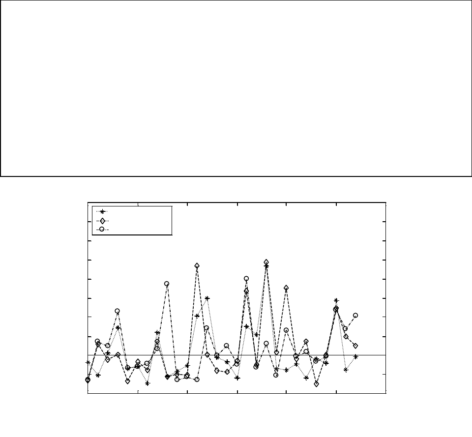
70
Box A4. Incorporating stage-specific productivity data in evaluations of abundance and productivity
trends: harvest estimates for coho salmon (Oncorhynchus kisutch) from coastal Oregon.
Estimates for (pre-harvest) recruits per spawner and escapement per spawner for coho salmon (O.
kisutch) from the Oregon coast illustrate the importance of considering productivity over different
portions of the life cycle when evaluating trends in abundance. Figures A4 and A5 show
estimates of recruits per spawner (R:S)—an estimate of productivity from spawners to “recruits,”
and spawners per spawner (S:S)—an estimate of productivity over the entire life cycle for three
gene conservation groups (GCGs, as defined by ODFW). For all three GCGs, R:S values have
been declining, while S:S values suggest a relatively stable pattern hovering near replacement.
Exploitation of coastal Oregon coho salmon has been historically high (40-90%), but it has been
declining in recent years (Figure A6). The failure of Oregon coho salmon populations to rebound
following the reduction in fishing mortality provides evidence that the production of pre-harvest
recruits has declined as well.
1965 1970 1975 1980 1985 1990 1995
0
0.5
1
1.5
2
2.5
3
3.5
4
4.5
5
North-Mid Coast
Umpqua
Mid-South Coast
Figure A4. Estimates of spawner:spawner production for Oregon coastal coho salmon (Oncorhynchus
kisutch) in three GCGs.
Spawners:Spawner
Year
Year
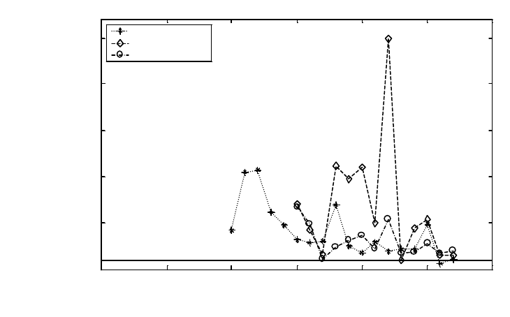
71
1965 1970 1975 1980 1985 1990 1995
0
5
10
15
20
25
North-Mid Coast
Umpqua
Mid-South Coast
Figure A5. Estimates of pre-harvest-recruit:spawner production for Oregon coastal coho salmon
(Oncorhynchus kisutch) in three GCGs.
Recruits:Spawner
Year
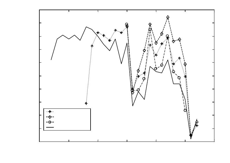
72
1965 1970 1975 1980 1985 1990 1995
0
0.1
0.2
0.3
0.4
0.5
0.6
0.7
0.8
0.9
1
North-Mid Coast
Umpqua
Mid-South Coast
OPI
Figure A6. Estimates of exploitation rates for three GCGs (North-Mid Coast, Umpqua, Mid-South Coast)
of Oregon coastal coho salmon (Oncorhynchus kisutch) and estimated total exploitation rate for
coho salmon in the Oregon Production Index Area based on analyses of coded wire tag
recoveries. Note the sharp decline in exploitation rate beginning in the late 1980's and extending
through the early 1990's.
Exploitation Rate
73
decades, but the harvest rate on this population has fallen substantially over the same time
period. This suggests that the population’s productivity may have declined as well (Waknitz et
al. 1995).
Note that in both examples discussed, we are unable to determine conclusively whether
the apparent decline in realized productivity is a consequence of declining intrinsic productivity
or due to increasingly strong density-dependent limitation. Mobrand et al. (1997) point out that
declines in either productivity or environmental capacity that affect a particular life-history stage
can exert similar overall effects on production through the entire life cycle. Estimates of stage-
specific productivity are therefore important for populations in which individuals’ use of
resources (e.g., duration of the life cycle spent in a given habitat) varies substantially among life-
history trajectories such that distinct life-history variants respond differently to changes in
environmental conditions that affect a specific life-history stage (e.g., Mobrand et al. 1997, Box
A5). Variation in population growth rates linked to differences in stage-specific dynamics
among alternative life histories has obvious implications for life-history diversity in a population
and vice versa (see following and “Diversity,” p. 19).
Understanding the dynamics of stage-specific productivity and how they affect
population viability may also be important for situations in which the dynamics of one life-
history stage dominate the dynamics of the entire life cycle. For example, a lack of habitat
suitable for overwintering parr is thought to limit smolt production in some populations of coho
salmon along the Oregon Coast to the degree that the parr experience a “bottleneck” with the
potential to mask productivity changes in earlier history stages or to limit the capacity of a
watershed to produce adults (Nickelson et al. 1992, Bradford et al. 1997). In this case, estimates
of intrinsic productivity and capacity for other life-history stages indicate the potential for the
population to increase in abundance should conditions that limit overwinter survival be
ameliorated.
Why ancillary data relevant to productivity are important
Ancillary data relevant to productivity include measurements of any characteristic having
clear links to reproductive success or survival, such as size of outmigrating smolts or size- and
age-at-maturity of adult fish. Incorporating such data into status evaluations is analogous to
examining stage-specific productivity, in that it may provide opportunity to detect changes that
may be of little importance in current population dynamics, yet may influence a population’s
overall productivity in the future.
One example where ancillary data were used as part of a risk assessment is the case of
Puget Sound/Strait of Georgia coho salmon (Oncorhynchus kisutch). In this assessment, a
sustained decline in size-at-return of adult fish was interpreted as an indication of increased risk
for Puget Sound/Strait of Georgia coho salmon populations (Box A6, Weitkamp et al. 1995). In
contrast, coho salmon populations from rivers along the outer coast of Washington State
exhibited consistent size-at-return. Additional risks related to changes in size-at-return were not
inferred for these populations. Declines in size-at-return and, in some cases, increases in age-at-
return have been documented in a number of salmon stocks (Ishida et al. 1993, Bigler et al. 1996,
Pyper and Peterman 1999). Either may be expected to reduce a population’s productivity.
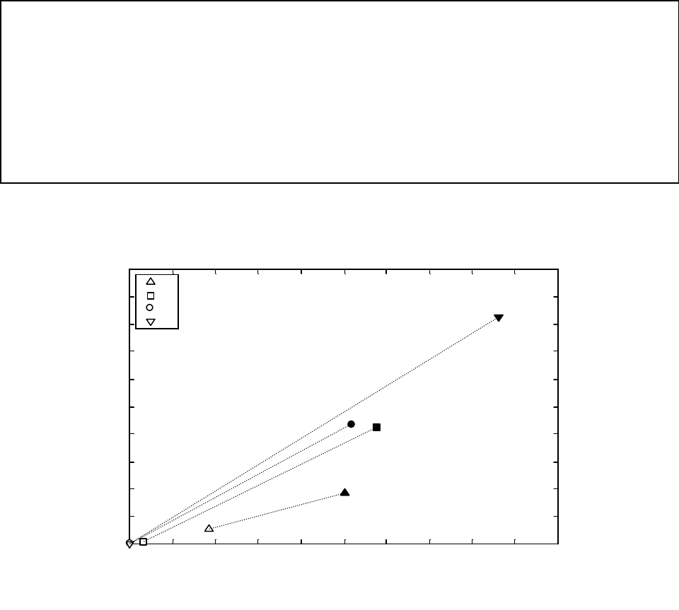
74
Box A5. Population dynamics in stage-structured populations and the fate of different life histories in a
population.
Mobrand et al. (1997) used a stage-structured model to illustrate how changes in environmental
conditions exert different influences on different life-history variants and how that may underlie
observed changes in the proportions of different life-history types in a population of spring run
chinook salmon (Oncorhynchus tshawytscha) in the Grand Ronde River (Figure A7). Life
histories that require different series of habitats experience environmental changes differently,
such that some strategies have been rendered entirely unviable by observed changes, while others
remain extant, although at depressed levels.
0 100 200 300 400 500 600 700 800 900 1000
0
0.2
0.4
0.6
0.8
1
1.2
1.4
1.6
1.8
2
a
b
c
d
Figure A7. Changes in parameters of a composite Beverton-Holt model for smolt yield as a function of
prespawner abundance for four putative life-history variants of spring chinook salmon
(Oncorhynchus tshawytscha) in the Grande Ronde River (redrawn from Mobrand et al. 1997,
Lestelle et al. 1996.). Filled symbols indicate estimated historical values; open symbols indicate
estimated current. Life history variants differ in timing and usage of freshwater habitats by
juveniles prior to downstream migration. They may be described roughly as follows: (a)
freshwater rearing through the summer and winter; following emergence occurs solely in the
upper reaches of the watershed where spawning takes place, (b) freshwater rearing occurs in
upper reaches of the watershed during the summer after emergence, followed by substantial
downstream displacement in the fall and overwintering in lower reaches of the river, (c)
freshwater rearing through the summer and winter; following emergence occurs just downstream
from habitats where spawning takes place—downstream dispersal occurs immediately after
emergence, and (d) early freshwater rearing occurs in the same pattern as in (c), but individuals
move downstream and leave the Grande Ronde watershed before the onset of winter.
Cumulative Productivity Index
Cumulative Capacity Index
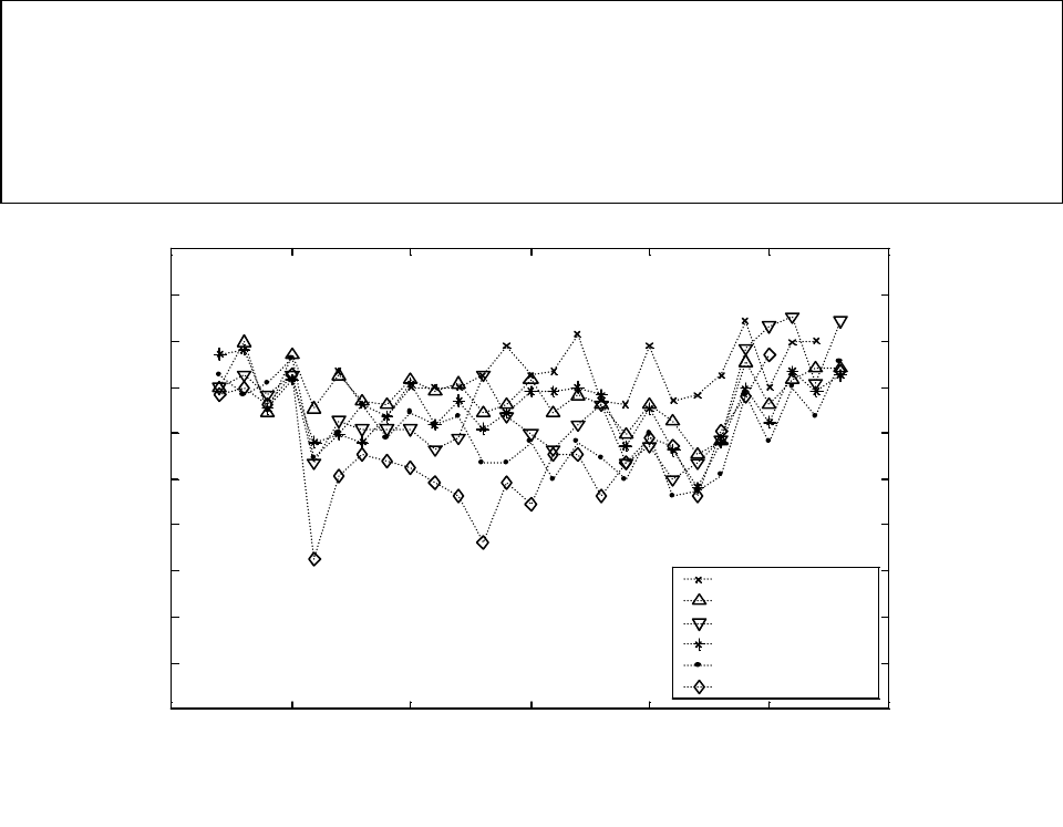
75
Box A6. Example of ancillary data relevant to population viability: trends in size of coho salmon from
different regions.
Figures A8 and A9 illustrate regional-scale trends in the size of adult coho salmon from
watersheds along the Pacific coast of Washington State and from watersheds emptying into Puget
Sound. Adult coho size was generally stable (and perhaps increasing) in coastal populations but
declined substantially in Puget Sound populations.
1970 1975 1980 1985 1990 1995 2000
1
1.5
2
2.5
3
3.5
4
4.5
5
5.5
6
CHEHALIS
QUINAULT
HOH
QUEETS
QUILLAYUTE
WAATCH/SOOES
Figure A8. Mean weights of coho salmon from rivers on the outer coast of Washington State. Rivers are
listed in order from south to north.
Mean Weight (kg)
Year
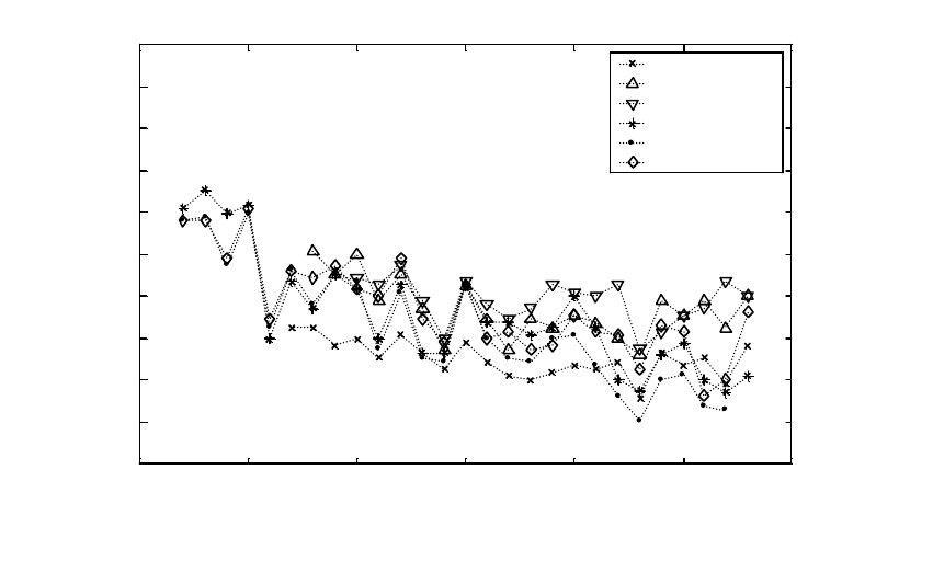
76
1970 1975 1980 1985 1990 1995 2000
1
1.5
2
2.5
3
3.5
4
4.5
5
5.5
6
NOOKSACK
SKAGIT
STILLIGUAMISH
DUWAMISH
PUYALUP
NISQUALLY
Figure A9. Mean weights of coho salmon from rivers in Puget Sound. Rivers are listed in order from
north to south.
Mean Weight (kg)
Year
77
Reduced size-at-maturity has obvious implications for individual fecundity and may
reduce individuals’ ability to reach upstream spawning grounds (Hinch and Rand 1998) or to dig
redds sufficiently deep to resist scour (DeVries 1997). Delayed reproduction subjects
individuals to greater pre-reproductive mortality risk, although this may be partially or
completely offset by increases in size (and hence fecundity) with age. Density-dependent
effects, possibly related to hatchery production or other production enhancement practices, have
been implicated as underlying causes for changes in size- and age-at-return (Ishida et al. 1993,
Bigler et al. 1996, Pyper and Peterman 1999). Size-selective harvest also alters the size- and
age-at-maturity in a salmon population—usually it reduces both because the selection is against
larger fish that mature at older ages (Healey 1986, Hankin 1993). In the latter case, productivity
may actually appear to increase at the cost of reduced life-history diversity (Hilborn 1985).
Estimating Population Growth Rate and Related Parameters
For applications to field data, both analytical approaches previously mentioned use time
series of estimated abundance for one or more life-history stages. Numerous methods have been
developed for estimating abundance at various stages in the salmonid life cycle (e.g., Hankin and
Reeves 1988, MacDonald and Smith 1980, English et al. 1992, Irvine et al. 1992, Dempson and
Stansbury 1991, Labelle 1994, Hilborn et al. 1999). Obviously, the quality of data used to
evaluate any parameter relating to population viability strongly affects the reliability and level of
uncertainty associated with the results of the analysis. Most techniques for estimating abundance
provide some estimate of the magnitude of observation error (the area-under-the-curve technique
for estimating spawner escapement is a notable exception, yet appears to outperform other
analyses in terms of accuracy [English et al. 1992, Hilborn et al. 1999]).
Our focus in this Appendix is on understanding the dynamics of individual populations—
this is explicitly assumed in our discussion of issues related to intrinsic productivity and density
dependence. Note that spatial structure can have profound implications for estimating
population growth rate, detecting important trends, and understanding population dynamics.
Spatial variation in population dynamics, particularly source-sink dynamics (sensu Pulliam
1988), can obscure trends in abundance (Brawn and Robinson 1996, Cooper and Mangel 1999).
A population’s dynamics may depend importantly on interactions with other populations during
life-history stages that share a common habitat (Bigler et al. 1996, Pyper and Peterman 1999,
Bjorkstedt SWFSC, unpublished results). Depending on rates of dispersal, metapopulation
structure may introduce non-linear dynamics in which a rapid “crash” to lower abundance or
even extinction may occur with little or no warning in the form of declining trends (Hanksi et al.
1994). Spatial structure is discussed in greater detail in “Spatial Structure,” p. 18.
Two issues relevant to data quality also bear special emphasis. First, failure to use
appropriate sampling designs may generate data that are not necessarily representative of the
population as a whole (e.g., counts from non-representative index reaches may reflect abundance
only in the most productive areas of a population’s range). This can strongly affect the validity
of parameter estimates and any viability assessment based on biased data and analysis. Meir and
Fagan (2000) find that systematic over- or-underestimates of abundance generally have little
impact on estimated extinction dynamics. However, they assume that such estimates, although
78
biased, are a simple multiplicative function of actual abundance while we are more concerned
here with cases in which abundance estimates are non-representative and reflect actual
abundance in a strongly non-linear way. For example population abundance estimates based
solely on counts in productive reaches may miss important declines in abundance as the
distribution of the population contracts into favorable habitats.
Second, analyses must be sure to avoid the influence of spurious autocorrelations arising
as a consequence of ignoring inherent temporal structure in the data. For example, some
salmonid populations exhibit limited life-history variability and thus have consistently
independent broodyear cycles (e.g., pink salmon, coho salmon in the southern part of the species
range, and sockeye salmon). Autocorrelation is likely to be apparent in abundance time series
for such populations, primarily at time lags corresponding to the average generation time. For
example, the persistence of dominant, sub-dominant, and weak broodyear cycles in many
sockeye salmon populations, the independence of even- and odd-year pink salmon runs, and the
disparity in abundance between broodyear cycles of coho salmon in central California are all
cases of spurious autocorrelation in abundance time series. Such autocorrelation, if unaccounted
for, tends to inflate the variance in the data. Unaccounted for autocorrelation also hinders
attempts to detect trends in abundance, estimate population growth rate, or discern underlying
functional relationships that describe population dynamics. Real autocorrelation, whether due to
intrinsic or extrinsic causes, has an important influence on extinction dynamics that bears on
assessments of population viability (Foley 1997).
Estimating population growth rate and changes in other parameters
Observational time series of abundance (or other characteristics of populations or
individuals) contain four sources of variation: 1) trend, 2) “interventions” or “epochs” marked by
unusual shifts in the underlying pattern or short-term departures from “regular” patterns,
respectively, 3) autocorrelation arising from intrinsic factors (e.g., density dependence,
sequential “baby-boom” signals at intervals that correspond to generation times) or extrinsic
factors (e.g., autocorrelated environmental forcing), and 4) random error (Barker and Sauer
1992, Thomas 1996). A number of statistical techniques exist for analyzing time series for
trends and other temporal patterns. Unfortunately, though the literature contains some guidelines
for using different analytical techniques (e.g., Berryman et al. 1988), there is no clear guidance
on how to approach time series analysis, and thus model selection remains a fairly subjective
process (Jassby and Powell 1990, Thomas 1996, and references therein). Therefore, we
recommend, as have others (Thomas 1996, Mangel and Hilborn 1997), pursuing multiple
approaches, testing the statistical power of alternative methods to discern temporal patterns of
interest, such as trends of a given magnitude and direction, and comparing the ability of
alternative models to describe the data.
Detailed analysis of temporal variation in a time series of abundance data might include
examining a suite of time series models that include various combinations of autoregressive
terms, moving averages, intervention terms, covariates, etc. However, available time series are
often short, particularly time series of abundances at scales appropriate to individual populations.
Therefore, we focus on simple approaches as follows, and touch upon relevant aspects of more
complicated temporal patterns that provide context for evaluating population viability in terms of
79
estimated population growth rate. The latter include addressing the influence of (non-spurious)
serial autocorrelation, detecting rapid, step-like changes in a time series through intervention
analysis, and analysis of singular or rare short-term events through epoch analysis. We focus the
discussion that immediately follows on approaches for estimating population growth rate and
issues that must be considered when doing so. However, much of what follows is also applicable
to detecting trends and other temporal patterns in other parameters relevant to productivity.
Estimating population growth rate and detecting trends
Productivity is typically measured as the ratio between the number of recruits from a
given broodyear and the number of spawners in that broodyear. Multiplying the abundance of
spawners by this ratio yields the number of recruits. By extension, the growth rate of a
population over multiple generations is, at least approximately, the product of productivities for
each generation. The mean growth rate of a population corresponds to the slope of a plot of
estimated abundance—following appropriate transformation—against time. For species that
have determinate semelparous life histories and non-overlapping generations, long-term
population growth rate is the simple product of population growth rate realized by each
generation. Life history variation and overlapping broodyear cycles in anadromous salmonids
requires more complicated analyses to estimate population growth rate, both for a single
generation and over a longer time period. Not surprisingly, developing accurate estimates of the
mean and variability in a population’s growth rate requires a) abundance estimates for a period
spanning several generations, and b) information on life-history variation in the population.
Regression-based approaches provide relatively simple means for estimating trends in
time series and are a useful way to analyze short time series. Thomas (1996) lists four general
types of regression analysis and discusses the advantages and disadvantages of each. To
estimate population growth rate, regression methods based on exponential (linear-multiplicative)
models are the simplest and most appropriate approach. In essence these analyses amount to
fitting an additive model to logarithmically transformed abundance data. For other parameters of
interest, such as changes in size-at-return, other regression models may be more appropriate
since the mechanism is not so clearly a multiplicative process as it is in the case of population
growth.
Regression analysis, using an exponential model, is an appealing approach to estimating
population growth rate because it is conceptually simple, corresponds to the multiplicative nature
of population dynamics, requires estimation of few parameters, and provides unbiased estimates
of the trend even in cases where interventions and autocorrelation are present in the data set
(Thomas 1996). Although temporal autocorrelation does not bias estimates of mean population
growth rate, autocorrelation does result in the breadth of confidence intervals regarding the
estimated trend being underestimated. This in turn, increases the likelihood of Type I error (i.e.,
erroneously reporting a non-existent trend or non-zero population growth rate) (Hurlburt 1984,
Bence 1995).
Regression analyses are also appealing due to the relative ease with which statistical
power can be estimated for regression analyses that are based on exponential models (Gerrodette
1987, 1991, Link and Hatfield 1990, Nickerson and Brunell 1997). Estimating statistical power
80
of an analysis allows the results to be evaluated. Evaluation focuses on the minimum effect that
is detected given the quality of the data (the number of observations, the precision of the
observations, etc.). Such information is essential for describing potential worst-case
consequences of proceeding as if the analysis accurately represented true conditions (Peterman
and Bradford 1987, Peterman 1990, Taylor and Gerrodette 1993, Korman and Higgins 1997).
Proceeding with a straightforward regression analysis on log-transformed abundance data
is not appropriate—life-history variation must be accounted for lest it bias an analysis. One
approach to dealing with difficulties arising from indeterminate life cycles and overlapping
generations is to estimate so-called “cohort replacement rates” (Botsford and Brittnacher 1998).
This may be accomplished by fitting the coefficients of a linear renewal equation (appropriately
structured to accommodate the population’s life history) to a time series of abundance estimates.
Doing so is relatively straightforward for populations in which life history is relatively inflexible
so that spawning runs are strongly and consistently dominated by a single-age class and
broodyear cycles are largely independent of each other (i.e., determinate, semelparous life
histories). In such a case, recruitment in one year is related to spawner abundance one
generation time in the past (e.g., two years for pink salmon, three for central California coho
populations, and four for some Fraser River sockeye populations). For populations with more
variable life histories (e.g., chum, chinook, and some populations of sockeye and coho),
estimating productivity and other population parameters requires models that account for
spawner age distributions and corresponding data to parameterize such models. For example,
estimates of recruitment used to estimate productivity for a population of chinook salmon with a
maximum age-at-return of 5 years old must equal the 3-, 4-, and 5-year old spawners originating
from the same broodyear. In many cases, there is little data on yearly variation in the age
composition of spawning adults, and a mean distribution based on a few years’ data, or data from
another population must be used. Doing this introduces extra uncertainty into estimates of
productivity, and may make it difficult to fit the model to abundance data (Botsford and
Brittnacher 1998). This problem has been addressed in at least two population viability analyses
for salmon populations. Botsford and Brittnacher (1998) estimated the distribution of cohort
replacement rates for winter-run Sacramento River chinook salmon using a linear renewal
equation approach under the assumption that population dynamics are density-independent.
Emlen (1995) used a more intensive, simulation-based approach to estimate parameters for a
density-dependent model for Snake River chinook salmon. Dennis et al. (1991) developed
regression-based estimates of the mean and variance of population growth rate from abundance
time series for use in a diffusion model for estimating extinction risk. This approach has been
adapted to indeterminate semelparous salmonid life cycles (CRI, 2000).
Detecting other pattern in time series: autocorrelation, interventions, and epochs
Serial autocorrelation in abundance time series (the dependence of each observation on
previous conditions) can accurately affect the ability to estimate the variance in population
growth rate or variation about trends in other parameters. Estimating autocorrelation in short
time series, typical of abundance data for salmonid populations is a difficult task. Bence (1995)
explores techniques for adjusting variances estimated from short time series data for the effects
of autocorrelation.
81
Intervention analysis provides a means of detecting rapid transitions between periods of
relative stability in a time series of data (Box and Tiao 1975). Hare, Francis, and colleagues
(Hare et al. 1999) used intervention analysis to identify periods of relatively high and low total
regional salmon production in Alaska, and coinciding, out-of-phase patterns of productivity in
the Pacific Northwest. Their analyses indicate that rapid shifts in salmon abundance and
production appear to be driven by changes in large-scale climate patterns that exhibit similar
step-like transitions. Note, however, that these results emerged from analyses conducted on
aggregated data sets that comprised many populations and thus, reduced the contribution of
observation error from any single population. Thus, intervention analysis is less likely to be
applicable to abundance time series for a single population because of the greater relative effects
of observation error in time series of abundance for individual populations.
Epoch analysis (Prager and Hoenig 1989, 1992) provides a technique for determining if
an unusual event in a time series is related to unusual environmental conditions. One example
that may prove useful in viability analysis is the case of identifying “outliers” that have a readily
identifiable mechanistic basis, such as the dramatic effect of El Niño-Southern Oscillation
(ENSO) events, on the productivity and abundance of a population.
Estimating intrinsic productivity and detecting density dependence
Much of ecology and fisheries science has focused on developing models and analyses to
estimate intrinsic productivity and the intensity of density-dependence in populations. Detailed
reviews of relevant analytical methods and applications may be found in Hilborn and Walters
(1992), Quinn and Deriso (1998), and the extensive literature on stock-recruitment relationships
(e.g., Iles 1994). Dennis, Taper and colleagues have developed statistical tests to detect density
dependence in time series of abundance estimates (Dennis and Taper 1994, Dennis et al. 1998,
and see Shenk et al. 1998 for discussion of the statistical validity of these tests). Examples of
simple models commonly used to describe spawner-recruit relationships in salmonid populations
include the Ricker (1954) and Beverton-Holt (1957) models. More complex models that
accommodate life-history structure and environmental or ecological covariates may be useful in
cases where data are sufficient to parameterize such models accurately. Also, analyses that
employ maximum likelihood methods and information criteria offer a way to simultaneously fit
and evaluate a large suite of models in order to identify the model form that best captures the
information in the data (Zeng et al. 1998). Such methods have been successfully demonstrated
in relatively data-rich systems but they have rarely been applied to salmon populations (but see
Hooten 1995 for examples based on spring and summer chinook from the Columbia River).
Bayesian analyses continue to be developed, and provide powerful techniques for estimating
parameters while accounting for correlation among parameters and uncertainty associated with
parameter estimates (Punt and Hilborn 1997, McAllister and Kirkwood 1998, Millar and Meyer
2000).
Critical assumptions
Fitting population dynamics models to time series of abundance requires two critical
assumptions: 1) that the real functional relationship between spawners and recruits that underlies
the observed data is stationary (Dennis et al. 1991, Hilborn and Walters 1992), and 2) that the
82
population is homogeneous (Hilborn 1985). For the assumption that the spawner-recruit
relationship is stationary to hold, the average dynamics and magnitude of variability in the
population must remain constant through time. Rapid changes in marine survival that appear to
accompany large-scale changes in oceanographic conditions (reviewed in Hare et al. 1999)
provide a natural case in which this assumption is violated. Anthropogenic actions, such as
ongoing degradation of freshwater habitats, also cause non-stationarity in a population’s
underlying dynamics. In some cases, the data support a model that treats productivity or
capacity as a function of time or environmental conditions in order to account for changes in the
underlying dynamics of a population. In an analysis for spring-run chinook salmon
(Oncorhynchus tschawytscha) in the Umpqua River, Ratner et al. (1998) used a model that
incorporated an exponential decline in available habitat over time to model the observed negative
trend in abundance. In another example, population dynamics of chinook salmon in the San
Joaquin River, predicted by a model that treated recruitment as a function of river flow
conditions better matched observed dynamics than did models that lacked environmental
covariates (S. Lindley, SWFSC, unpublished data). Statistical analyses that use information
criteria to guide model selection may help determine appropriate model structure (e.g., density
dependence or independence, temporally variable or constant parameters, etc.) as well as
estimate parameter values from population abundance data sets (Zeng et al. 1998, Lele et al.
1998).
The assumption that the population is homogeneous requires that: 1) the data
are from a single, well-mixed population rather than a collection of populations that exhibit
different demographic parameters (Ricker 1973, Hilborn 1985) or a population occupying a
spatially heterogeneous habitat, and 2) that life-history variants do not represent independent
groups within a putative population. When analyzing data from a structured population,
differences in productivity or capacity among subpopulations and life-history variants must be
taken into account, otherwise productivity is likely to be overestimated, particularly if the
population is already in a depleted state (Hilborn 1985). This may have drastic implications for
less productive populations and life-history variants that, not surprisingly, are more vulnerable to
depletion. If subpopulations that comprise a population are linked by substantial migration,
depletion of less productive populations may be less of an issue as more productive populations
may be expected to subsidize less productive neighbors. Likewise, if life-history variation is not
strongly heritable, the component of the population exhibiting a more productive life-history
strategy may produce some offspring that exhibit alternative, less productive life histories. This
in turn would subsidize less productive elements of life-history diversity within a population.
However, heritability of life-history parameters, such as age-at-maturation (Hankin et al. 1993),
may make any changes in population dynamics, related to shifts in life-history variation, difficult
to counter or reverse.
Bias and methods for correcting it
Even when the assumptions required for fitting a simple population model to abundance
data are satisfied, natural variability and measurement error may introduce substantial biases into
spawner recruit estimates. In general, such analyses overestimate intrinsic productivity and the
intensity of density-dependence, and underestimate serial autocorrelation (Walters and Ludwig
1981, Walters 1985, 1990, Korman et al. 1995, Myers and Barrowman 1995). Use of estimates
83
of population dynamics parameters biased in this way to estimate extinction risk will estimate
risks that are much lower than actually exist in a population. An analysis of sockeye salmon
stocks suggests that such biases appear to be strongest for populations with low productivity and
strongly autocorrelated residual error (Korman et al. 1995). Thus, for populations that exhibit
dynamics consistent with increased risk of extinction, biases in estimates of population dynamics
parameters may lead to substantial underestimation of such risk and overestimation of population
viability.
There are at least four methods for countering the biases inherent in analyses of
functional relationships in the dynamics of a population: 1) using formulae that have been
developed to partially correct for such biases (e.g., Walters 1990), 2) determining the
relationship between parameter estimates and observation error using simulation methods and
subsequently, using extrapolation to predict parameter values for data in which observation error
is absent (Solow 1998, and references therein), 3) attempting to reduce unexplained process error
by identifying and accounting for environmental signals in recruitment data (e.g., Welch 1986,
Kope and Botsford 1988, Iles and Beverton 1998, S. Lindley, SWFSC unpublished data), and 4)
simulating abundance data from population dynamics models that include parameters estimated
from data, re-estimating the models from the simulated data, subtracting the different initial
parameter estimates, and repeating the cycle as necessary (Ratner et al. 1997).
Analyses that incorporate stage-specific dynamics
Simple population dynamics models ignore any age- or stage-structure that may exist in a
population, and are unable to capture important differences in how the abundance of different
population components respond to changes in environmental conditions. However, in many
cases, extending simple population models to accommodate life-history structure is a
straightforward, albeit difficult, process that requires more data to parameterize the resulting
models (for examples cast in diverse modeling frameworks, see Tuljapurkar and Caswell 1996
and references therein). Structured-population models allow analyses to incorporate information
on stage-specific dynamics and thereby generate a more complete picture of a population’s
dynamics (see Emlen 1995, Botsford and Brittnacher 1998, Ratner et al. 1997). Models for
structured populations (e.g., Mousalli and Hilborn 1986, Caswell 1989, Cushing 1996, Emlen
1995, Yamauchi and Matsumiya 1997, Bjorkstedt 2000) provide a framework for assessing
potential population viability implications of changes in factors affecting stage-specific
production (e.g., Mobrand et al. 1997). Such analyses typically consist of evaluating the
sensitivity or elasticity that a structured-population model (in matrix form) exhibits in response
to small changes in productivity parameters at a given life stage (Caswell 1989, Grant and
Benton 2000). This is a powerful technique, but must be used with some caution to be sure its
results do not conflict with biological reality (Mills et al. 1999).
Productivities estimated for discrete life-history stages are often treated as independent of
productivity during other parts of the life cycle (e.g., freshwater v. marine survival [Bradford
1995]), and therefore taken as an indication of the “performance” of a population in a given
habitat. This assumption may not always hold (see Bjorkstedt 2000 and references therein),
which may have important implications for evaluating population viability and recovery options,
84
particularly for populations that interact in common habitats during some portion of the life cycle
(Bjorkstedt, SWFSC, unpublished results).
Analyses of populations that include naturally spawning hatchery fish
The ESA and NMFS policy both focus on natural population abundance. The VSP
definition is consistent with this in stating that a population that is dependent on hatchery
production is not a viable one. Given the tight connection between abundance and productivity,
it is therefore necessary to estimate natural productivity of hatchery-influenced populations
rigorously. Special problems arise when attempting to estimate productivity for a population in
which fish produced in hatcheries constitute a substantial proportion of the naturally spawning
adults. Not surprisingly, estimates of natural productivity are very sensitive to errors in
estimating the relative abundance of naturally produced and hatchery fish. Not surprisingly,
valid estimates of natural productivity are impossible to obtain for supplemented populations in
which the abundance of naturally-produced and hatchery-produced fish on the spawning grounds
are not estimated separately.
The influence that naturally spawning hatchery fish have on natural productivity is
governed by two factors: 1) relative reproductive success of naturally spawning hatchery fish and
naturally born fish, and 2) density dependence in reproductive success, which in turn depends on
the relative competitive abilities of hatchery- and naturally-produced fish and the proportion of
each in the spawning population (Fleming and Gross 1993). Natural Return Ratios is defined as
the number of naturally-produced fish that are born during a given broodyear and subsequently
return to spawn, divided by the total number of fish on the natural spawning grounds (including
naturally spawning hatchery fish) in that broodyear (Busby et al. 1994). The definition has been
used as a measure of natural productions in previous population assessments. However, the
calculation of NRR implicitly assumes density-independent population dynamics. This
assumption detracts from the value of NRR as a measure of natural production. Box A7
discusses how the NRR concept may suitably be extended to analyzing populations that include
naturally spawning hatchery fish. Note that in practice and in these analyses, offspring of
naturally spawning hatchery fish, by virtue of having survived in the natural environment, are
counted as natural spawners when they return.
From a purely demographic perspective, theoretical models provide some guidance for
what proportion of a naturally spawning population may be of hatchery origin for that population
to exhibit dynamics largely independent of hatchery influence. Hastings (1993), using a simple
density-dependent model for two populations linked by dispersal, demonstrated that at least
under some conditions, the abundance in one population remained uncorrelated with that of the
other population, provided that immigration did not exceed approximately 10% of the receiving
population (see Kendall and Fox 1998 for a more thorough treatment of this model). From an
explicit metapopulation perspective, Dreschler and Wissel (1997) demonstrated that extinction
dynamics for a local population could be treated as independent of larger scale dynamics so long
as immigration remained at least at an order of magnitude smaller than the growth rate of the
local population. Based on these two models, an initial guideline for the proportion of naturally
spawning hatchery fish, in a population that is consistent with the natural population having
independent dynamics, is approximately 10%. This corresponds to a (density-independent) NRR

85
Box A7. Estimating productivity in populations that include naturally spawning hatchery fish.
Estimating natural productivity from a population that includes naturally spawning hatchery fish
requires information on the origin of spawners producing natural fish, i.e., the number of
spawners born in the natural environments and the number of hatchery strays spawning in natural
habitats. One measure of productivity typically calculated from such data is a Natural Return
Ratio (NRR), calculated as:
( )
HN
N
SS
R
NRR
+
= (A7a)
Where
N
R is the number of recruits from parents spawning in the natural environment (regardless
of parental origin) that were born in a given broodyear, and the parental population giving rise to
those recruits is made up of naturally-born fish,
N
S , and hatchery fish,
H
S , returning to the
spawning grounds. Note that (A7a) implicitly assumes that hatchery fish have reproductive
success equivalent to that of wild fish. Also, by rearranging the expression to solve for the
number of recruits
(
)
HNN
SSNRRR += (A7b)
(and noting the similarity between the calculation of NRR and models of density-independent
population growth), it is seen that the NRR explicitly disregards the possibility that density-
dependence could affect a population. For these two reasons, the uncritical use of NRR in
evaluating the productivity of a population is not recommended.
The sensitivity of NRR to violation of the two assumptions implicit in its calculation, may be
addressed using simple, but more complete, models that incorporate productivity and density-
dependence as functions of the abundance of both “hatchery” and “natural” spawners. A
Beverton-Holt model for a wild population affected by hatchery strays may be written as
( )
++
+=
HN
HNN
SgS
SfSR
β
α
1
)( (A7c)
whereα is the intrinsic productivity of the (wild) population, β describes the intensity of density-
dependence affecting the population,
f
indicates the relative (proportional) reproductive success
of hatchery fish,
g
describes the (proportional) competitive effectiveness of hatchery fish under
whatever density-dependent mechanisms limit reproductive success. (Note that g itself may be a
function of the natural:hatchery composition of the spawning population [Fleming and Gross
1993], a complication that, for simplicity, we do not address here.) An analogous Ricker model
may be written as
(
)
{
}
HNHNN
SgSSfSR ++=
βα
exp)( . (A7d)
Note that if f = 0 and g = 0, the wild population has dynamics independent of hatchery influence.
Similarly, if
0=f
but
0>g
, hatchery fish on the spawning grounds effectively reduce the
productivity of the wild population but do not contribute to the next generation. If both f > 0 and
g > 0, hatchery fish may contribute to natural production, but may limit the production of
offspring from parents of natural-origin through density-dependent limitation or by matings
between naturally- and hatchery-produced spawners. A case where hatchery fish contribute to
wild production but do not exert a density-dependent effect (e.g.,
0>f
and
0=g
) is

86
biologically implausible (it is possible for hatchery fish to contribute to production without a
density-dependent effect, but only if the wild component of the population also exhibits density-
independent dynamics, e.g.,
0=
β
, in which case the value of g is irrelevant). The
effect of increased density-dependent limitation of per capita productivity may be especially
important if the number of strays is sufficient to cause the number of fish in the spawning
population to exceed the population’s normal carrying capacity (see discussion of pseudo-sinks in
“Spatial Structure,” p. 18).
An analysis of estimated spawners (partitioned by origin) for summer steelhead (Oncorhynchus
mykiss) from the Wenatchee River illustrates the sensitivity of NRR calculated with Equation
(Figure A10) to the reproductive success of hatchery fish relative to that of natural fish (Figure
A10). Analyses using Ricker models, that incorporate different ways hatchery strays may affect
the production of wild returns indicate that hatchery- and natural-born fish may have similar
contributions to natural production of Wenatchee River summer steelhead (Figure A11). Note
that this analysis does not attempt to estimate f or g—rather, this example is intended only to
illustrate a proof of concept for incorporating more comprehensive population dynamics into
estimation of natural production.
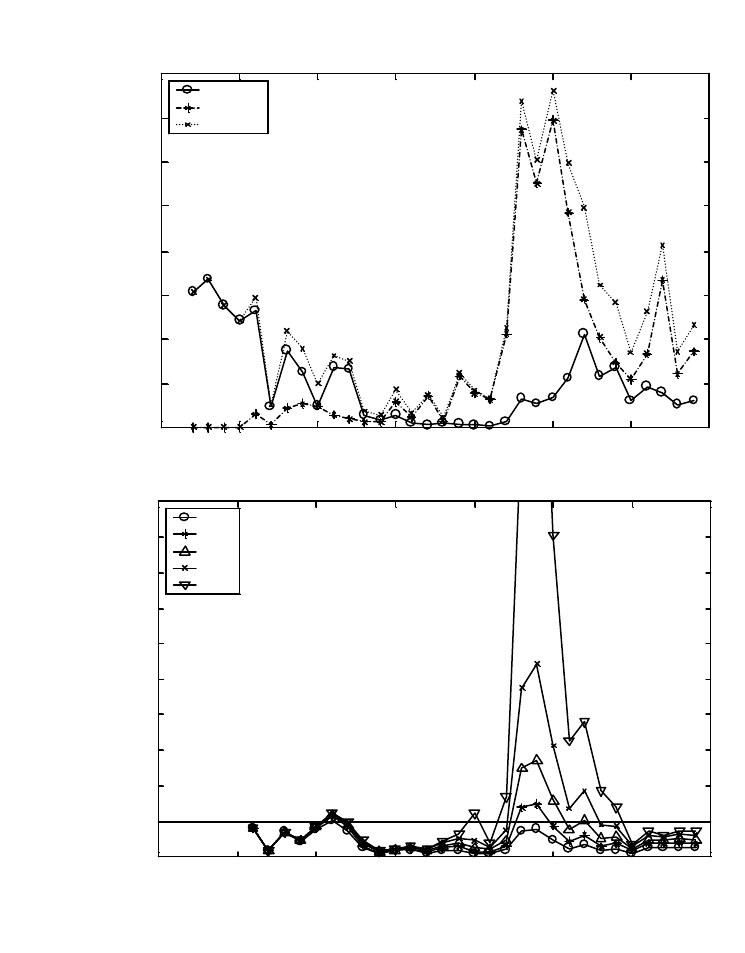
87
1960 1965 1970 1975 1980 1985 1990 1995
0
1000
2000
3000
4000
5000
6000
7000
8000
natural
hatchery
total
Year
1960 1965 1970 1975 1980 1985 1990 1995
0
1
2
3
4
5
6
7
8
9
10
1.00
0.50
0.25
0.10
0.00
Figure A10. Top panel: estimated spawner escapement for Wenatchee River summer steelhead
(O. mykiss), broken down into naturally spawning hatchery fish and spawners of natural origin
(data from StreamNet). Bottom panel: Natural Return Ratio (NRR) calculated for a range of
values describing the relative reproductive successes of hatchery- and natural-origin spawners
(NRR reaches a maximum of 16 in calculations based on the assumption that hatchery strays
contribute nothing to natural returns). In this example, the population's dynamics are assumed to
be density-independent, and each estimate includes estimated production from 2-6 year old
spawners (crudely based on data from Howell et al. 1985, as cited in Busby et al. 1996).
NRR Spawner Abundance
Year
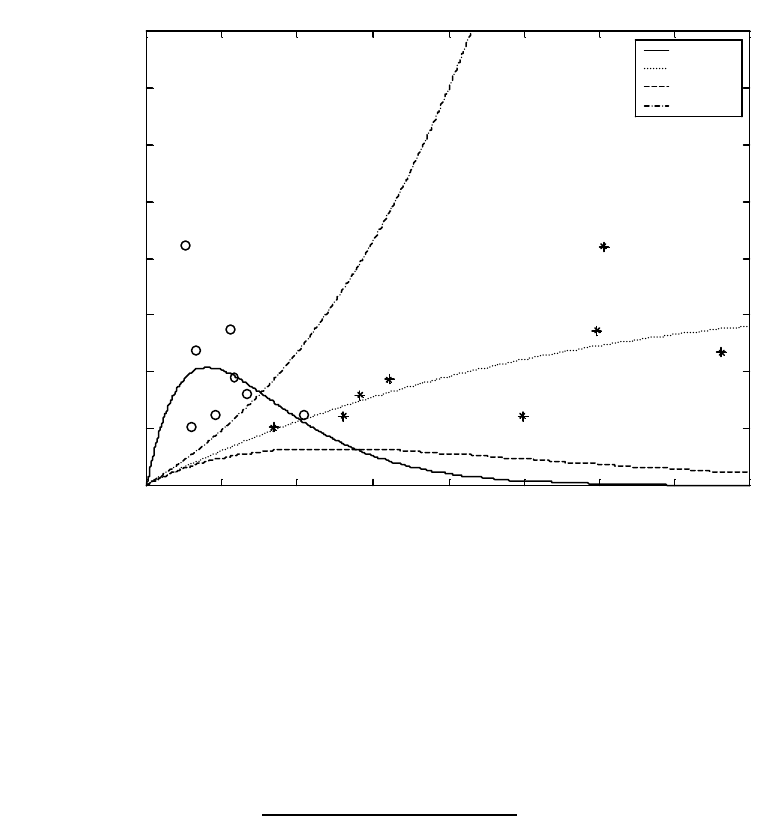
88
0 1000 2000 3000 4000 5000 6000 7000 8000
0
500
1000
1500
2000
2500
3000
3500
4000
f=0; g=0
f=1; g=1
f=0; g=1
f=1; g=0
Figure A11. Examples of Ricker-type spawner-recruit models that include the influence of naturally
spawning hatchery fish in different ways, fitted to data for Wenatchee River summer steelhead
(Oncorhynchus mykiss) for 1984-1994. This time period was selected in an attempt to avoid
violating the assumption of stationarity in the underlying dynamics—this period is marked by
roughly consistent returns of natural spawners. Open circles are data for natural returns plotted
against spawners of natural origin. Asterisks are data for natural returns plotted against combined
spawners of both hatchery and natural origin. Each curve describes the best-fit model (Equation
A7d) under a particular set of assumptions about the contribution and density-dependent effect of
naturally spawning hatchery fish (see text for details). The parameters for the different curves are
f g α β .
0 0 3.47 -1.2×10
-3
1 1 0.33 -7.7×10
-5
0 1 0.36 -4.1×10
-4
1 0 0.40 2.0×10
-4
Note that the case of f = 1 and g = 0—that is, a case in which a fish may contribute to
production without exerting a density-dependent effect given that density dependence is
significantly affects the population’s dynamics—is biologically implausible. (If density
dependence is non-existent, i.e., β = 0, the value of g is irrelevant.) This example is
intended as an illustration only, and no attempt has been made in this example to find best
fits for f and g in these models.
Recruits
Spawners

89
Box A8. Population growth rate and related parameters guidelines.
1. A population’s natural productivity should be sufficient to maintain its abundance above the
viable level. A population meeting or exceeding abundance criteria for viability should, on average,
be able to replace itself. That is, spawner:spawner ratios or cohort-replacement ratios should
fluctuate around 1.0 or above. Natural productivity is typically measured as the ratio of naturally-
produced spawners born in one broodyear to the number of fish spawning in the natural habitat during
that broodyear. Population abundance estimates at other life-history stages may also be used,
provided such estimates span the entire life cycle (e.g., smolt to smolt estimates).
2. A viable salmonid population that includes naturally spawning hatchery fish should exhibit
sufficient productivity from naturally-produced spawners to maintain population abundance at
or above viability thresholds in the absence of hatchery subsidy. In a strict sense, this guideline
suggests that the mean Natural Return Ratio (NRR) for a viable population should fluctuate around
1.0—indicating negligible hatchery influence on the population. In a practical sense, the requirement
that a viable population be demographically independent of a hatchery population suggests that a
viable population’s mean NRR not be less than approximately 0.9, but this estimate neglects other
issues related to the influence of hatchery fish on natural production. A viable population should not
exhibit a trend of proportionally increasing contributions from naturally spawning hatchery fish.
3. A viable salmonid population should exhibit sufficient productivity during freshwater life-
history stages to maintain its abundance at or above viable thresholds—even during poor ocean
conditions. A population’s productivity should allow it both to exploit available habitat and exhibit a
compensatory response at low population sizes. When spawner abundance is below the long-term
mean, there should be a corresponding increase in per capita smolt production, even though such an
increase may not suffice to offset declines in marine survival.
4. A viable salmonid population should not exhibit sustained declines in abundance that span
multiple generations and affect multiple broodyear-cycles. “Sustained” declines are those that
continue longer than the typical lag in response associated with a population’s generation time. Thus,
sustained declines differ from rapid transitions between one stable level and another (e.g., changes in
abundance related to large-scale, low frequency environmental forcing such as those related to
oceanic regime shifts). They also differ from short-term, severe perturbations in abundance (such as
those related to strong El Niño events) that are followed by relatively rapid recovery.
5. A viable salmonid population should not exhibit trends or shifts in traits that portend declines
in population growth rate. Changes in such traits, such as size and age of spawners, that affect
population growth rate are often more easily and precisely quantified than are changes in abundance
and thus, may provide earlier indication of declining population growth rate. For example, reduced
size of mature individuals in a population may indicate reduced fecundity, lessened ability to reach
spawning grounds, a decreased capacity for constructing redds that are deep enough to resist bed
scour, or other factors that contribute to reduced production of offspring. Likewise, increasing age-at-
return may reduce a population’s intrinsic productivity by exposing adults to greater pre-reproductive
spawning risk.
6. Population status evaluations should take into account uncertainty in estimates of population
growth rate and productivity-related parameters. To estimate long-term trends and spawner-
recruit ratios, it is important to have an adequate time series of abundance. Unfortunately, such time
series, when they exist at all, are often short and contain large observational errors, or both. These
constraints may greatly limit the power of statistical analyses to detect ecologically significant trends
before substantial changes in abundance have occurred.
90
of 0.9. It must be emphasized, however, that establishing criteria for natural production in
hatchery-influenced populations must take into account factors besides the demographic
measures discussed here, and are likely to require more conservative criteria than that suggested
by the preceding argument.
Spatial Structure
Introduction
Any viability evaluation must consider spatial structure within a population (or group of
populations) because spatial structure affects extinction risk in ways that may not be readily
apparent from short-term observations of abundance and productivity (Hanksi and Gilpin1997,
Tilman and Lehman 1997, Cooper and Mangel 1999). The spatial structure of a population
refers both to the spatial distributions of individuals in the population and the processes that
generate that distribution. Spatial structures that consist of groups of individuals in discrete
patches are often generically referred to as “metapopulations,” though the term has assumed a
variety of meanings over the years (Hanski and Simberloff 1997). A population’s spatial
structure depends fundamentally on habitat quality and spatial configuration, and the dynamics
and dispersal characteristics of individuals in the population.
Because many of the processes that affect small population extinction risk (e.g., genetic
risks and demographic stochasticity) depend primarily on breeding structure, we will focus on
spawning group distribution and connectivity. Restricting the discussion to spawning groups is a
practical step in evaluating population viability, but it should be noted that spatial structure is
likely to be important during all life-history stages.
Spatial structure in spawning aggregations of salmonids is a natural consequence of the
species’ ability to home to natal watersheds, natal tributaries within watersheds, and (potentially)
natal reaches within tributaries. Homing provides a mechanism for maintaining a hierarchy of
reproductive isolation among groups of fish that reflects the dendritic structure of watersheds
(Policansky and Magnuson 1998). Straying (i.e., the return of individuals to freshwater habitats
other than that in which they were born—Table A1) offsets both the demographic and genetic
isolation of such groups. We refer to groups of fish that are relatively reproductively isolated
from other groups within a population as “subpopulations”.
In this section we first briefly describe general spatial structure patterns that may occur
and then discuss a few simple spatial models that illustrate why spatial structure is an important
parameter in assessing population viability. (This will not be an exhaustive discussion of the
spatial models that may apply to salmonids.) We conclude the section by summarizing the
current understanding of spatial structure in salmonids and describing how spatial structure can
be assessed. The effect of spatial structure on genetic processes is discussed in the “Diversity”
section, p. 101.
91
General Spatial Patterns
Several schemes for classifying population spatial structure have been developed (e.g.,
Harrison and Taylor 1997, Gilpin 1993). Figure A12 illustrates some potential spatial patterns
described in the general ecological literature. The dynamic spatial pattern of a population
depends on the movement patterns of individuals (straying) and the structure of the habitat. The
spatial patterns shown in Figure A12 all assume that the habitat is divided into discrete “patches”
surrounded by unsuitable habitat. Patch attributes that affect spatial patterns are size, number,
quality, spatial distribution, and stability. As panel B shows, fluctuations in abundance can also
affect the observed spatial pattern. A single population may simultaneously exhibit multiple
types of spatial structure, depending on the spatial and temporal scale examined. For example, at
a large spatial scale a group of fish may show a source-sink dynamic, while at the local scale of
an individual patch, the group may be panmictic.
In a panmictic population, every mature individual is equally likely to mate with every
other mature individual of the opposite gender. In a patchy panmictic population, the habitat is
divided into discrete patches, but movement (straying) is so high that the breeding pattern is
panmictic and no subpopulations are formed. The term “classic metapopulation” refers to the
type of population structure first modeled by Levin (1969). In a classic metapopulation, the
habitat is divided into discrete patches, all of which are identical in every way and migration is
equally likely among all patches. Subpopulation extinction and the colonization of empty
habitats drive the dynamics of a classic metapopulation. There is a substantial amount of
theoretical literature on metapopulations and they are discussed in some detail as follows. What
we are referring to as a “structured population with no extinction” is a variant of a classic
metapopulation in which there is sufficient straying so that subpopulations are “rescued” from
extinction by migrants, but straying is insufficient to create a patchy panmictic population.
Island-mainland systems consist of a single large stable population (“mainland”) surrounded by
smaller subpopulations (“islands”) that are prone to extinction. Because of the asymmetry in
subpopulation size, straying is also asymmetrical, with most migration occurring from the
mainland to the islands. Source-sink populations are similar to island-mainland systems in that
migration is asymmetrical. However, in source-sink systems, the asymmetry occurs because
highly productive source populations send a relatively large number of migrants to the sink
subpopulations, which are not self-sustaining and would deterministically go extinct in the
absence of migrants from the source (Pulliam 1988).
Why Spatial Structure is Important
Metapopulation theory
Levins (1969) coined the term metapopulation to describe a “population of populations.”
Here, we will refer to a metapopulation as a set of subpopulations, to avoid confusing it with the
definition of population used in this document and various definitions in the literature. Groups
of populations (as we define them) may also act as metapopulations at larger temporal and
spatial scales than the within population level. This possibility is discussed in the section on
ESU viability (“Viable ESUs,” p. 125).
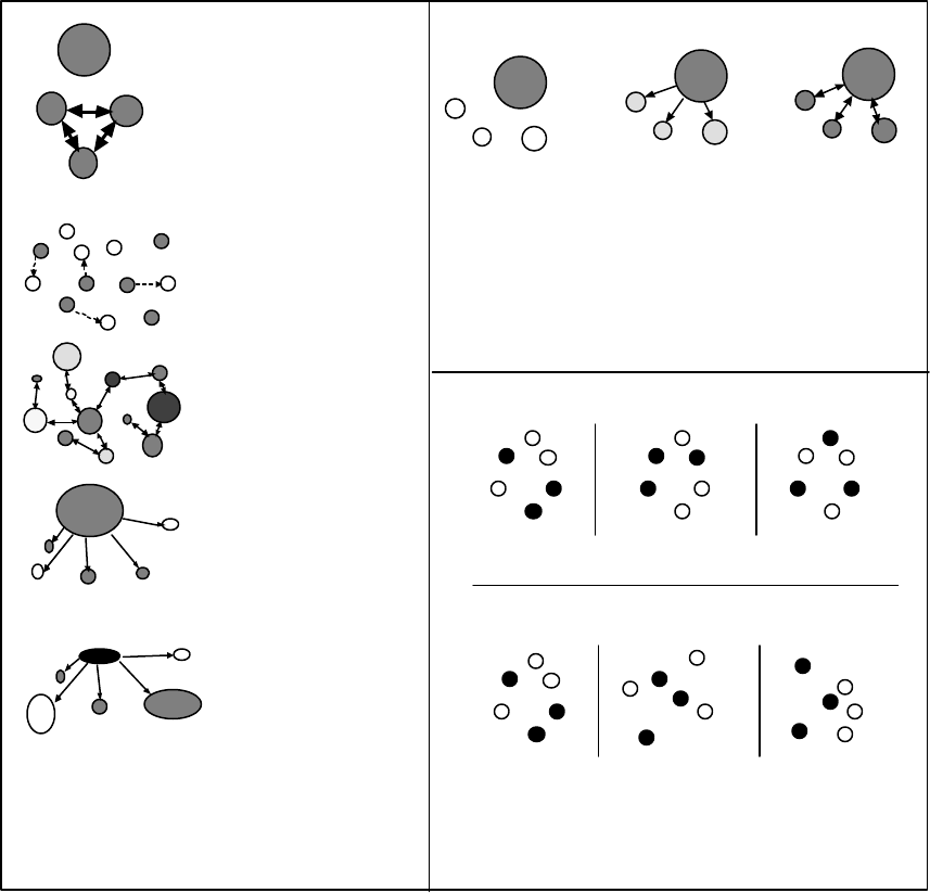
92
homogeneous panmictic population
patchy panmictic population
“classical”
metapopulation
Low survival years -
single panmictic
population
Moderate survival year -
source sink population
High survival years -
structured population
Panel B: Temporal changes in
population structure
Panel A: “Traditional”
classification of population
structure
Panel C: Static vs. dynamic habitat
Static habitat
Dynamic habitat
Time 1 Time 3Time 2
Time 1 Time 3Time 2
structured populaton
with no extinctions
source-sink population
island-mainland population
Figure A12. Theoretical types of spatially structured populations. Panel A shows a “traditional” type
classification scheme that does not consider correlated environmental effects that impact all
subpopulations, nor does it explicitly consider the physical dynamics of the habitat patches
themselves. The circles indicate habitat patches, with the size of the circle indicating the size or
capacity of the patch, and the degree of shading indicating the density of the subpopulation—
white indicating an empty patch and black indicating a high density patch. The arrows indicate
levels of migration, with thick arrows indicating high migration, thin arrows moderate migration,
and dashed arrows indicating intermittent migration. Panel B shows how spatial structure may
oscillate over time as a result of correlated environmental changes in survival or productivity
among subpopulations. Correlated environmental changes might result, for example, from annual
variation in ocean survival that affects all subpopulations. Panel C shows two potential habitat
patterns. In a static habitat, the location of suitable patches remains constant over time, though
patches may or may not always be occupied. In a dynamic habitat, the location of suitable habitat
continually changes, and so the location of subpopulations must also change.

93
The “classic” Levins metapopulation model (Levins 1969, 1970) assumes the
environment is divided into discrete patches of suitable habitat. These patches may represent
different streams or stream sections that may be occupied by different subpopulations. Two
processes, subpopulation extinction and patch colonization via migration from occupied patches,
interact to create a dynamic pattern of occupied and empty patches. The dynamic equation of the
Levins model is:
eppmp
dt
dp
−−= )1(
Where p is the fraction of occupied patches, m is the rate at which strays colonize new patches,
and e is the rate at which subpopulations go extinct (because of natural habitat dynamics or
intrinsic subpopulation dynamics). By solving the equation for the equilibrium proportion of
occupied patches, it can be shown that a metapopulation will persist only when the colonization
rate exceeds the extinction rate (m>e).
This simple model makes several key predictions relevant to the conservation of
endangered species. First, at equilibrium, some suitable patches will remain unoccupied. Using a
slight modification of the Levins model, Hanski et al. (1996) explored the ecological
consequences of destroying suitable (though perhaps temporarily unoccupied) patches. The
basic dynamic model to determine minimum viable metapopulation size is:
( )
epphmp
dt
dp
−−= ,
Where p, m and e are as above and 1-h is the fraction of habitat patches destroyed by human
alteration. At equilibrium, the metapopulation persists (i.e., equilibrium p > 0) only when h<e/m.
This leads to a general rule of thumb which Hanski et al. (1996) called the Levins Rule: “A
necessary and sufficient condition for metapopulation survival is that the remaining number of
habitat patches following a reduction in patch number exceeds the number of empty but suitable
patches prior to patch destruction.”
A second key result of the metapopulation modeling is that there may be substantial time
lags between the destruction of habitat patches and observable decreases in abundance or
population growth rate (Levins 1969, Wennergren et al. 1995, Hanksi et al. 1996, McCarthy et
al. 1997, Tilman and Lehman 1997, Cooper and Mangel 1999). If habitat patch destruction
focuses on suitable, but temporarily unoccupied patches, population abundance may remain
relatively stable until subpopulations in occupied patches begin to go extinct. The rate at which
subpopulations go extinct may be slow relative to the time scale over which trends in abundance
are evaluated. The productivity of the population (spawners per spawner) may also appear to be
relatively stable after habitat patch destruction because the problem that habitat destruction
creates is a lack of suitable targets for colonization, not declining productivity in occupied
patches. Metapopulations that persist for some period of time but are ultimately doomed to
extinction because there is an insufficient number of habitat patches for them to inhabit, have
been referred to as “the living dead” (Hanski et al. 1996).
A third result is that the metapopulation persistence depends critically on the colonization
rate which, in salmonids, is tied to straying patterns among patches. A decrease in movement
among patches could cause the subpopulation extinction rate to exceed the patch colonization
rate—causing metapopulation extinction. Since straying in salmonids tends to decrease with

94
distance, increasing the inter-patch distance may result in a non-viable salmonid population.
The metapopulation models presented make the simplifying assumptions that all patches
are equal except with regard to occupancy, every patch is equally accessible to every other patch,
and internal patch dynamics are irrelevant.
9
It is not clear to what extent the Levins' type
metapopulation models apply to salmonids (or any organism for that matter (Harrison 1994,
Harrison and Taylor 1997). As we discuss in the following, many of the essential features of
salmonid biology such as discrete, dynamic habitat patches and limited straying, are captured in
the models. However, the patch-occupancy type models may poorly describe salmonid
population spatial structure if straying is very high. Hanksi and others (Day and Possingham
1995, Gyllenberg and Hanski 1997, Gyllenberg et al. 1997, Hastings and Harrison 1994) have
explored variations of the basic metapopulation model presented. Their results indicate that the
number of suitable patches is likely to be an important predictor of overall metapopulation
survival, even when many of the strict Levins’ assumptions are relaxed. As long as: a) the
habitat is broken up into discrete patches, b) there is some limited straying among patches, and
(c) we assume that there is some natural process driving subpopulation turn-over, we must
consider the number of suitable habitat patches available to the population and recognize that the
population may not be able to survive if that number is reduced. Note that the individual patches
themselves do not have to remain constant, only the mean number of them. Patch turnover is a
natural process and conservation approaches that seek to preserve specific patches of suitable
habitat in perpetuity may be doomed to failure (Reeves et al. 1995).
Source-sink dynamics
Habitat patches differ in quality and this is reflected in productivity differences among
subpopulations. Data on coho salmon in the Snohomish River, WA is consistent with this
hypothesis, since some patches consistently show higher numbers of spawners per spawner than
other patches (Figure A13). This differentiation among habitat patches can lead to a source-sink
dynamic in which some subpopulations (the sources) have a higher productivity and are self-
sustaining, while other subpopulations (the sinks) have a lower productivity, are not self-
sustaining, and only persist because there is an influx of strays from the source population
(Pulliam 1988). Schlosser and Angermeier (1995), citing work by Reimers (1973) on Oregon
chinook, argue that source-sink dynamics may be common in lotic systems and care must be
taken to protect source populations. Cooper and Mangel (1999) discuss the theoretical and
management implications of source-sink dynamics in salmonids and they also note that an
important goal in a source-sink system is protection of source populations.
It can be very difficult to identify source and sink populations. Simple observations of
abundance do not reveal source-sink dynamics; sink subpopulations can be much larger than the
source population. The key issue in defining sources and sinks is productivity. Subpopulation
productivity is impossible to document by examining only adult spawners unless it is clear what
9
In a classical metapopulation, subpopulations are assumed to have independent probabilities of extinction.
Independent extinction risk is one of the criteria in our definition of a population, not a subpopulation. However, the
population criterion of independent extinction risk refers only to intrinsic factors (e.g., demographic stochasticity). If
subpopulation turnover is driven by extrinsic factors (e.g., habitat dynamics), subpopulations may show independent
extinction risks, even though they are demographically coupled.
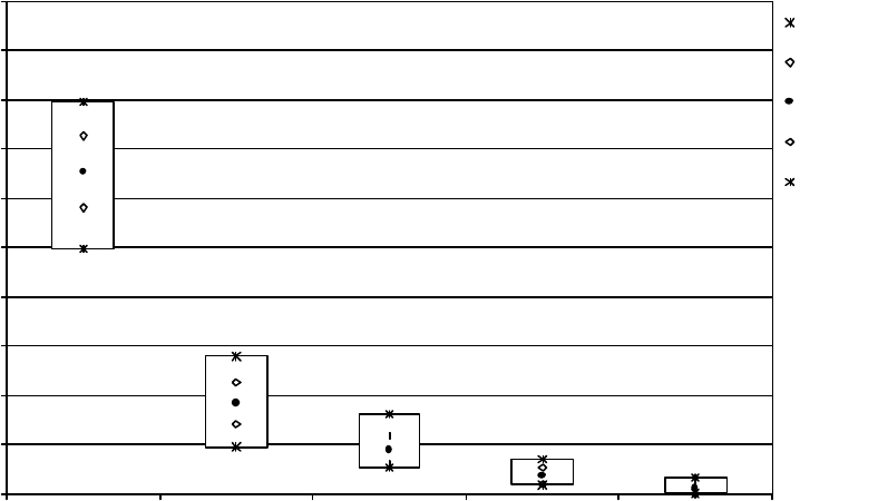
95
Snohomish River coho escapement distribution
sorted by most to least productive index reaches (1984 to 1998)
(Source: WDFW spawner survey escapement estimates)
0%
10%
20%
30%
40%
50%
60%
70%
80%
90%
100%
1 through 11 12 through 22 23 through 33 34 through 43 44 through 54
Ranked index reaches
Percent total escapement
minimum
std dev
average
std dev
maximum
Figure A13. Productivity estimated as spawners per spawner by index reach for coho in the Snohomish
River, WA (Bilby et al. 1999). The data is consistent with the idea that some reaches have
consistently higher productivity than others do. However, without data on the straying patterns
among reaches, it is difficult to determine whether or not spawner per spawner data reflects reach
specific productivity.

96
proportion of the spawners returning to a patch hatched there. Such data generally are not
available. Another way to document subpopulation productivity is to look at the number of fry
produced per spawner. This approach is only valid if fry can be attributed to a specific
subpopulation. That is, sampling must be conducted before fry from one subpopulation mingle
with those from other subpopulations. Using an analogous approach to study bird populations,
Brawn and Robinson (1996) examined the productivity of neotropical migrants in the mid-west
by observing the number of fledglings produced per breeding female. Most populations they
surveyed were actually sink populations, despite apparently stable abundance counts spanning
decades.
In many salmonid systems, hatchery populations may serves as sources and wild
populations as sinks. For example, in the upper Columbia steelhead ESU, over 50% of the
spawners in the natural spawning grounds are estimated to be first generation hatchery fish
(Chapman et al. 1994). Under the population growth rate guidelines, such a system would not be
considered a VSP.
Importance of patch spacing
In terrestrial species, adequate migration corridors are important because they provide
physical connection between subpopulations so that colonization of patches can equal or exceed
extinction. Several recent efforts in conservation biology have focused on the pros and cons of
“migration corridors” (Fahrig and Merriam 1994, Hess 1996, Lidicker and Koenig 1996,
Simberloff et al. 1992). Since the frequency of straying tends to decrease with distance from the
natal patch (see following), patch spacing is the primary factor determining “migration
corridors” in salmonids
10
. If habitat patches are too widely spaced, then patch extinction or
destruction may outpace colonization. Thus, the spatial arrangement of habitat patches must be
considered when assessing spatial structure, because it affects the probability that colonization
can occur should empty (but suitable) habitat become available. This process has been explored
in a number of theoretical “stepping-stone” models (e.g., Kareiva 1990, Bascompte and Sole
1996). In an empirical study of a bull trout metapopulation, Dunham and Reiman (1999) found a
decrease in patch occupancy with increasing distance from an occupied patch. In their generic
salmonid metapopulation model, Cooper and Mangel (1999) used (without empirical validation)
an exponential function to describe the decrease in straying probability with increasing distance.
The model shows subpopulation persistence decreasing with distance from a source population,
indicating the need to consider the spatial distribution of patches in evaluating population
viability.
As illustrated in Figure A12, populations may expand into new habitat patches during
times of high productivity (for example during periods of high ocean survival). This may occur
even if the quality of adjacent patches is lower than in the “core” patch. These “marginal”
10
All anadromous fish start the return to spawn from the ocean. If a spawning habitat patch is accessible from the
ocean, fish from every subpopulation in a population should have physical access to the site (assuming there are no
phenotypic differences among subpopulations regarding migratory ability). Thus, physical barriers are less likely to
limit straying among existing subpopulations in salmonids than in terrestrial systems, and the primary factor limiting
straying among subpopulations is the extent of homing fidelity and the physical (or temporal) distance between
patches.
97
patches may still contribute to population abundance during favorable years and thus help buffer
the population from extinction. However, if patches are too far apart, populations may not be
able to expand to new patches in times of high productivity. Thus, the spacing of habitat patches
that rarely contain fish may affect population viability.
Fragmented habitats
Populations that were historically panmictic may currently exist as a collection of
subpopulations because their habitat has been fragmented (Reeves et al. 1995, Harrison and
Taylor 1997). If there is little straying among the fragments, each of the subpopulations
effectively becomes their own demographically independent population, which may be too small
to be viable. Provided there is some level of straying among fragments, a new metapopulation
structure may be established. Although a novel metapopulation structure may be stable, stability
is difficult to verify. We therefore recommend that historical structure be considered as a default
goal for spatial structure (Guideline 5). It is important to note that restoring a fragmented habitat
to continuity would reduce the total number of habitat patches but increase the total amount of
habitat area. This provides an exception to Guideline 1, which states that the number of suitable
patches should not be declining in a viable population.
Assessing Spatial Structure
To determine the applicability of patch dynamic models (e.g., the Levin’s model) to
salmonid conservation, it is first necessary to determine whether subpopulations and patches
even exist, and if they do, at what spatial and temporal scales. In this section, we briefly review
information on spatial structure in salmonids and indicate the types of data needed to evaluate a
population’s spatial structure.
Straying
Subpopulations are delineated by degree of reproductive isolation; therefore straying
estimates can be very useful in estimating population structure. The entire suite of tools
discussed in the section “Identifying Populations” (p. 38) can be used to estimate straying
patterns and the degree of reproductive isolation among subpopulations. Perhaps the best
method for directly measuring straying patterns involves studying tagged individuals.
Unfortunately, such studies are scarce. In Table A1, we summarize studies that directly measure
the rate of straying among groups of fish. Many studies report large ranges in stray rate—
reflecting either great diversity in stray rates among species and populations, very imprecise
estimates of stray rate, or both. Most of the published stray rate studies examined a fairly broad
spatial scale, using hatchery fish, or both. So it is difficult to draw conclusions about within-
population site fidelity among natural spawners. One general conclusion that can be reached
from the salmonid stray rate data is that straying declines with distance from natal streams,
though the exact shape of the dispersal curve is unknown. At a very local spatial scale,
salmonids are not expected to show site fidelity because homing to the particular square meter of
gravel where they hatched is likely to be maladaptive. Because very small-scale habitat changes
are common, the particular spawning site where an individual hatched may no longer exist when
98
the fish returns. A completely inflexible homing strategy would not result in successful
spawning. At the other extreme, the studies clearly show a pattern of homing fidelity at the scale
of relatively large river systems such that it is possible to make reasonable estimates of
population boundaries. It is at the within-population scale that data on homing fidelity are
particularly lacking. Data on straying (or dispersal) is notoriously difficult to get for any species,
a fact that has important implications for obtaining reliable estimates of extinction risk
(Wennergren et al. 1995). This lack of reliable stray pattern estimates is perhaps the greatest
deterrent to applying quantitative spatial viability models in salmonids.
Habitat dynamics
Stream surveys suggest that salmonids spawn in discrete patches interspersed with areas
containing no spawners. For example, data on the spawning distribution of spring-run chinook
salmon in the Grande Ronde River (Figure A14) indicate that the basin is divided into a number
of discrete spawning areas. We have not conducted an analysis of this system, but it is
reasonable to hypothesize that these groups of fish may each represent one or more
subpopulations occupying discrete patches. This map shows that spatial resolution in the
available data is limited; data at a finer resolution would undoubtedly reveal discrete spawning
patch locations within each of the shaded regions. Although spawner distribution data provide
some information about the spatial distribution of spawning habitat, it is important to note that it
is not valid to equate the two (i.e., fish may mistakenly spawn in unsuitable habitat and,
conversely, suitable habitat may not contain any fish). In addition, it is not clear whether the
current spawner distribution represents a stable structure or an unstable artifact of recent human
habitat disruptions.
As an alternative to using spawner distribution surveys to describe habitat structure, the
spatial distribution of the habitat itself can be directly measured. By surveying streams for a
number of physical and biotic characteristics associated with spawning habitat, it is theoretically
possible to produce a map of suitable spawning areas (e.g., CLAMS project). The difficulty with
this approach arises when attempting to identify the characteristics and evaluate the quality of
suitable habitat. Several quantitative indices that attempt to correlate habitat characteristics with
salmonid productivity have been developed (e.g., NMFS PFC matrix of pathways and
indicators), however the accuracy of these indices is difficult to evaluate. Many efforts to
estimate habitat spatial distribution and quality rely on subjective expert opinion (e.g., Cedar
River survey [Cedar River HCP 1999]); this may be accurate in some cases, but it is difficult to
apply uniformly. In a recent effort to quantify habitat structure, NMFS researchers (Bilby et. al.
1999) have correlated habitat attributes with coho salmon production in Washington’s
Snohomish River, and they have identified physical attributes that are useful for evaluating
habitat structure. The study reveals a patchy distribution of spawning in the Snohomish River
system and suggests that some habitat patches consistently have higher productivity than others
do (Figure A13). There are a number of possible interpretations of this pattern, but one obvious
possibility is that habitat patches vary greatly in quality.
At some temporal and spatial scale, physical processes change the spatial structure of
spawning habitat. Natural processes constantly rearrange river substrates, alter river depths, or
completely change the course of a river (Benda 1994, Reeves et al. 1995). Bisson et al. (1997)
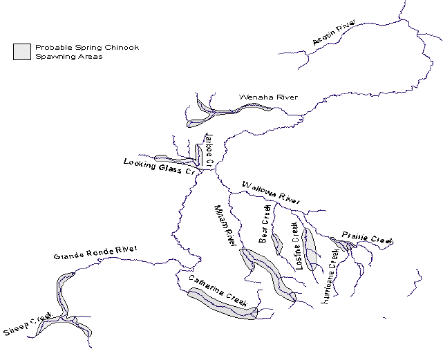
99
Figure A14. Map of probable spring chinook spawning areas in the Grande Ronde basin. (Redrawn from
map in NWPPC 1994.)

100
Box A9. Spatial Structure Guidelines.
1. Habitat patches should not be destroyed faster than they are naturally created. Salmonid
habitat is dynamic, with suitable habitat being continually created and destroyed by natural processes.
Human activities should not decrease either the total area of habitat OR the number of habitat patches.
This guideline is similar to the population growth rate criterion—i.e., a negative trend has
deterministically negative affects on viability—though the relationship between decreasing number of
patches and extinction risk is not necessarily linear.
2. Natural rates of straying among subpopulations should not be substantially increased or
decreased by human actions. This guideline means that habitat patches should be close enough
together to allow appropriate exchange of spawners and the expansion of the population into under-
used patches during times when salmon are abundant (see Guideline 3). Also, stray rates should not
be much greater than pristine levels because increases in stray rates may negatively affect a
population’s viability if fish wander into unsuitable habitat or interbreed with genetically unrelated
fish.
3. Some habitat patches should be maintained that appear to be suitable or marginally suitable,
but currently contain no fish. In the dynamics of natural populations, there may be time lags
between the appearance of empty but suitable habitat (by whatever process) and the colonization of
that habitat. If human activity is allowed to render habitat unsuitable when no fish are present, the
population as a whole may not be sustainable over the long term.
4. Source subpopulations should be maintained. Some habitat patches are naturally more productive
than others. In fact, a few patches may operate as highly productive source subpopulations that
support several sink subpopulations that are not self-sustaining. Protecting these source patches
should obviously be of the highest priority. However, it should be recognized that spatial processes
are dynamic and that sources and sinks may exchange roles over time
5. Analyses of population spatial processes should take uncertainty into account. In general, there
is less information available on how spatial processes relate to salmonid viability than there is for the
other VSP parameters. As a default, historic spatial processes should be preserved because we
assume that the historical population structure was sustainable but we do not know whether a novel
spatial structure will be.
101
provide a table of the temporal frequency and spatial extent of disturbance events likely to affect
salmon habitat. The data on coho salmon in the Snohomish River suggest that the location and
quality of habitat patches can remain stable for more than 15 years at a time (Figure A13),
though it is difficult to determine how much these results reflect other river basins or species.
The dynamic nature of spawning habitat provides an added challenge in assessing spatial
structure. To evaluate viability, we must not only understand the current habitat structure, but
also anticipate its future patterns of occupancy and suitability.
VSP Guidelines: Spatial Structure
While it is easy to demonstrate theoretically that spatial structure is an important
parameter for assessing population viability, it is difficult to develop generic guidelines
regarding structure. If habitat occurs in discrete patches, but fish stray randomly to any patch,
then any changes in habitat quantity or quality are likely to be quickly reflected by changes in
population abundance and productivity. In such a case, it would not generally be necessary to
extensively evaluate spatial structure and the resources for doing so could be used elsewhere.
However, if straying is limited to the point where something approaching a classical
metapopulation structure is created, or habitat productivity generates a source-sink dynamic,
knowledge of a population’s spatial structure could be crucial. Although the following
guidelines are designed to apply to a broad range of populations, a key recommendation is to
invest in empirical research on spatial processes in order that more refined guidelines may be
developed and the crucial question of spatial scale can be addressed.
Diversity
This section discusses the relationships between diversity and population viability. In
this context, diversity refers to the distribution of traits within and among populations. These
range in scale from DNA sequence variation at single genes to complex life-history traits. The
goal of this section is to summarize what is known about diversity’s importance to salmonid
population viability. The section “Population Size” (p. 53) discusses the relationship between
population size and some factors, such as inbreeding and genetic drift, that affect genetic
diversity. This section focuses on diversity itself as a factor affecting population viability, as
opposed to simply viewing it as an attribute of effective population size.
Types of Diversity
The scientific literature extensively reviews and discusses salmonid diversity—both
within and among populations (recent reviews include Ricker 1972, Groot and Margolis 1991,
Taylor 1991, Healey and Prince 1995, Weitkamp et al. 1995, Busby et al. 1996, Gustafson et al.
1997, Myers et al. 1998 and Johnson et al. 1999). Salmonid traits often exhibit considerable
diversity within and among populations. This variation has important effects on population
viability. Some of these varying traits are anadromy, morphology, fecundity, run timing, spawn
timing, juvenile behavior, age at smolting, age at maturity, egg size, developmental rate, ocean
distribution patterns, male and female spawning behavior, physiology and molecular genetic

102
characteristics. Of these traits, some (such as DNA or protein sequence variation) are completely
genetically based, whereas others (such as nearly all morphological, behavioral, and life-history
traits) usually vary as a result of a combination of genetic and environmental factors (see Ricker
1972, Taylor 1991 and Healey and Price 1995 for reviews). Box A10 provides several examples
of variation of traits within and among populations of chinook salmon.
Why Diversity is Important
In a spatially and temporally varying environment, there are three general reasons why
diversity is important for species and population viability. First, diversity allows a species to use
a wider array of environments than they could without it. For example, variation in adult run and
spawn timing allows several salmonid species to use a greater variety of spawning habitats than
would be possible without this diversity (see reviews in Groot and Margolis 1991). Second,
diversity protects a species against short-term spatial and temporal changes in the environment.
Fish with different characteristics have different likelihoods of persisting, depending on local
environmental conditions. Therefore, the more diverse a population is, the more likely it is that
some individuals would survive and reproduce in the face of environmental variation. For
example, all of the Pacific salmonid species except pink salmon vary with respect to age at
maturity (see reviews in Groot and Margolis 1991). This diversity has the effect of spreading a
population out over several years, thus protecting the population against poor environmental
conditions or catastrophic losses in any particular year. Third, genetic diversity provides the raw
material for surviving long-term environmental changes. Salmonids regularly face cyclic or
directional changes in their freshwater, estuarine, and ocean environments due to natural and
human causes. Genetic diversity allows them to adapt to these changes. For example, it has
been hypothesized that river-type sockeye salmon are essential for species survival during times
of glacial advance, when the more highly adapted (and currently more abundant) lake-forms go
extinct in areas covered by ice (Wood 1995).
Factors that Affect Diversity
Genetic diversity within and among populations is primarily affected by five forces: mutation,
selection, drift, recombination, and migration
11
(reviewed by Hartl and Clark 1989). Phenotypic
diversity is influenced by the genes that guide development, by random environmental effects,
and by developmental processes that allow the same genotype to display different phenotypes in
different environments (phenotypic plasticity). Until the middle of this century, many salmon
biologists believed that observed phenotypic differences among populations were most likely
due to phenotypic plasticity expressed by more or less genetically uniform individuals (discussed
by Ricker 1972). Under this assumption, it would be difficult to argue that there is a strong
relationship between diversity and population or species viability. This is because any individual
would presumably be able to express the range of observed phenotypes under appropriate
environmental conditions, although non-genetic diversity might still be important in buffering
populations against environmental stochasticity. Over the last half of the century, the paradigm
has shifted toward the view that much of the observed diversity within and among salmonid
11
These are the primary forces that are most relevant to our discussion. There are additional forces that affect
genetic variation, such as transposable elements and retroviruses.
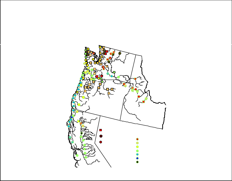
103
Box A10. Examples of Diversity. Below are three brief examples illustrating trait diversity within and
among populations of chinook salmon.
Example A10-1. Peak spawn timing of chinook salmon in the Pacific Northwest and California. Figure
A10-1a illustrates spawn timing diversity among chinook salmon in different streams. We do not
know to what extent these differences are due to genetic or environmental variation, or both.
W - Winter Run (May/June)
Fall Run
Summer Run
Spring Run
W
Aug
Dec
Nov
Oct
Sept
Feb
Time of Peak Spawning
Jan
Figure A10-1a. (Reproduced from Myers et al. (1998, Figure 10).)
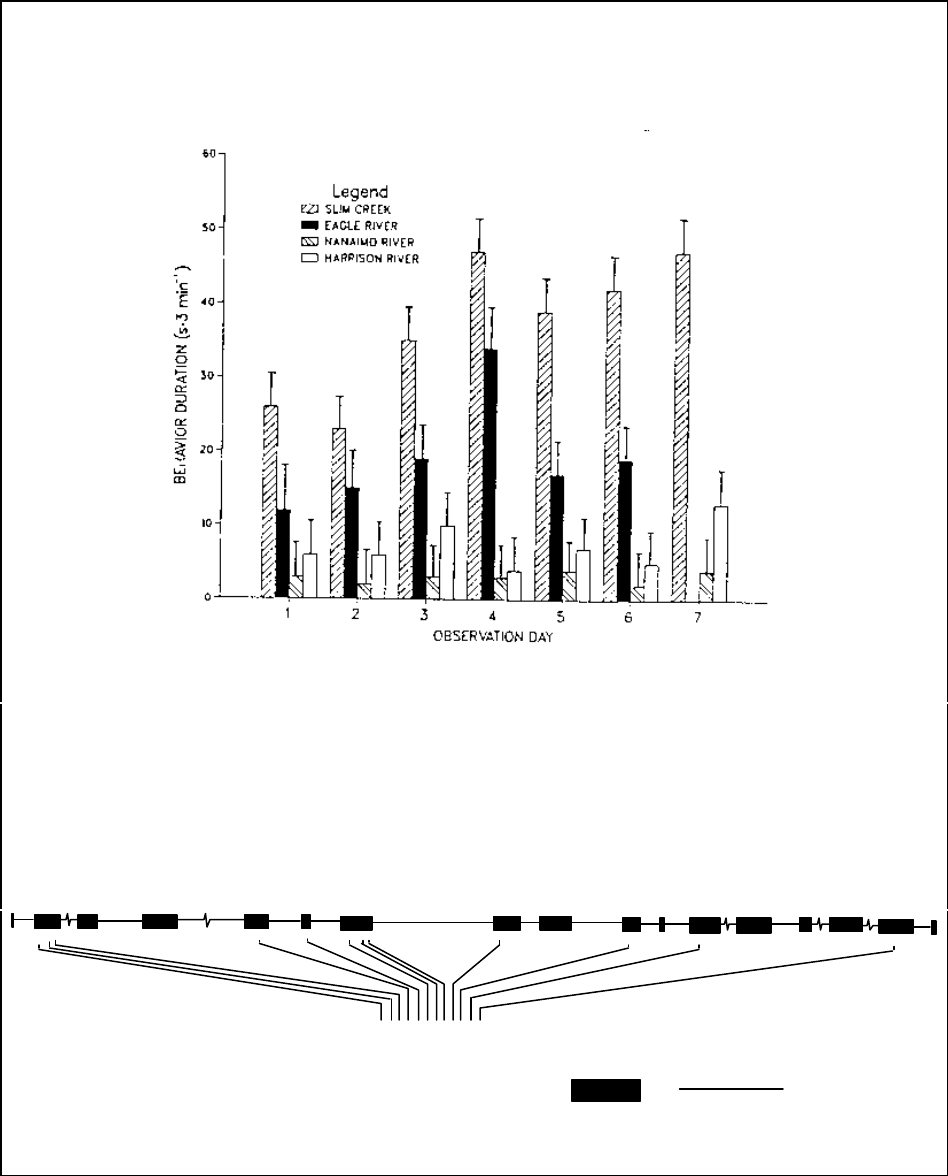
104
Example A10-2. Behavioral variation in chinook salmon fry. Taylor (1988) studied behavioral differences
between several British Columbian chinook salmon populations. Figure A10-2a shows the
duration of “lateral displays” (an agonistic behavior) among chinook salmon fry whose parents
originated from four different British Columbia streams. The fry were hatched and reared in a
common environment, suggesting that the differences have a genetic basis.
Figure A10-2a. (Reproduced from Taylor (1988).)
Example A10-3. DNA sequence variation at the transferrin gene. Figure A10-3a shows the nucleotide
sites at the transferrin gene that vary among six chinook salmon individuals sampled from the
Imnaha River, Oregon. The top part of the figure is a schematic diagram of the exon/intron
structure of the gene, and the bottom part of the figure shows nucleotide sites that vary among the
six individuals sampled. Only variation in exon sites is shown. “R,” “Y,” “K,” “M,” “S,” and
“W” refer to A/G, C/T, G/T, A/C, G/C, and A/T heterozygotes, respectively.
Exon Intron
1 2 3 4
5
6
7 8 9
10 11
12
13
14 15 16
17
Ot-Imnaha-05 CGTGACAGAAAT
Ot-Imnaha-24 SGGAGTTTCCGT
Ot-Imnaha-33 CGKRRYWKMMRT
Ot-Imnaha-34 SKTRRYWKMMRW
Ot-Imnaha-79 SGKRRYWKMMRT
Ot-Imnaha-83 CKTRRYWKMMRW
Figure A10-3a. Data from Ford et al. (1999).
105
populations is both genetically and environmentally influenced, and therefore at least partially
heritable. Under this paradigm, diversity takes on more significance because it would be
difficult to replace once lost. There is considerable evidence to show that observed patterns of
diversity are at least party based on genetic factors (reviewed by Ricker 1972, Taylor 1991):
salmonid homing behavior means that different spawning groups are likely to be at last partially
reproductively isolated from each other, thus promoting genetic differentiation (e.g., Foerster
1936, Quinn and Fresh 1984, Labelle 1992, Quinn 1993), 2) common garden experiments have
demonstrated that observed differences between populations often remain when fish from
different populations are reared in a common environment (e.g., Taylor 1988, Tallman 1986,
Clark et al. 1992, Withler et al. 1987); 3) breeding studies that allow the genetic variance of
specific traits to be estimated have shown that many of the traits that differ within and among
natural populations are genetically variable (reviewed by Tave 1993); and 4) population surveys
of variation in protein and DNA sequences have directly shown that salmonids are genetically
variable within and among populations (e.g., Parkinson 1984, Gharret et al. 1987, Reisenbichler
and Phelps 1989, Utter et al. 1989, Wood et al. 1994, Weitkamp et al. 1995, Myers et al. 1998,
Gustafson et al. 1998, Ford 1998).
Although it is now generally accepted that much of the observed diversity within and
among salmonid species has at least some genetic basis, the adaptive importance of this diversity
is still uncertain. Natural selection is one force that could create differences among populations,
but differences could also arise from non-adaptive processes such as genetic drift (e.g., Adkinson
1995). Box A11 provides several examples of (apparently) adaptive diversity, and Ricker
(1972), Taylor (1991), and Healey and Prince (1995) provide many examples of differences
among salmonid stocks that appear to be adaptive. There are many cases of management
concern, however, where there may simply be no data on the adaptive significance of observed
differences among populations (or even whether there are phenotypic or genetic differences
among populations). It is also important to note that the absence of phenotypic differences
between two populations does not mean that the two populations are not locally adapted. For
example, the populations may differ genetically in ways that allow the expression of a common
phenotype in two distinct environments (see Example 1 in Box A11), or they may simply differ
in traits that have not been examined. There are management and conservation costs associated
with both, incorrectly assuming that adaptive differences among populations exist when in fact
they do not or incorrectly assuming that no differences exist when in fact they do. In the former
case, unnecessary time or scarce resources might be spent on management actions designed to
conserve differences that do not exist or are not important, while in the latter case important
genetic variation could be lost.
Risks to Diversity
Actions that affect patterns of mutation, selection, drift, recombination, and migration all
have the potential to reduce or alter adaptive patterns of diversity. Mutation and drift are
primarily influenced by the genetically effective size of a population, and are discussed in
“Population Size” (p. 53). This section focuses on how selection and gene flow affect patterns of
diversity.

106
Box A11. Examples of adaptive diversity. In his review of local adaptation in salmonids, Taylor (1991)
used the following criteria to determine if there was evidence that a trait was locally adaptive: 1)
the trait must have a genetic basis, (2) differential expression of the trait must result in differences
in survival or reproductive capacity, and 3) a selective mechanism must be demonstrated. Several
examples for salmon populations that at least come close to meeting these criteria are discussed
as follows.
Example A11-1. Differences in development time in chum salmon. Healey and Prince (1995) present an
example of local adaptation drawn from work on three spawning groups of chum salmon studied
by Tallman (1986) and Tallman and Healey (1991, 1994). The three groups spawn at different
times in two streams, Bush and Walker Creeks, that empty into Ladysmith Harbor on Vancouver
Island less than 2 km apart from each other. There are two spawning runs in Bush Creek, an
early run with peak spawning in late October and a late run with peak spawning in late
November. The Walker Creek group has a still later peak, spawning in mid-December. Despite
these differences in spawn timing, the timing of fry emergence and downstream migration is
similar among the three groups, with Walker Creek fry actually migrating slightly earlier than the
Bush Creek fry. Differences in the development rates remain when the groups are brought into a
common environment, which suggests that these differences are genetically based. The groups
maintain their phenotypic differences despite fairly high levels of straying among them (Tallman
and Healey 1994), evidence that the differences among the populations are selectively
maintained. No selective mechanism has been convincingly demonstrated, but Tallman and
Healey (1991) hypothesize that conditions in Ladysmith Harbor may select for an optimal time of
fry outmigration despite differences in spawning time and incubation temperature among the
runs. If so, this is intriguing because it provides an example of genetic adaptation for phenotypic
uniformity (Tallman and Healey 1991).
Example A11-2. Fry migratory behavior. Upon emerging from the gravel, fry in many river systems must
migrate upstream or downstream to rearing areas (reviewed in Groot and Margolis 1991).
Several studies have demonstrated that in some populations the tendency to migrate in a
particular direction is innate. The data in the following table are from Raleigh (1971); they show
the percentage of fry that moved upstream or downstream in an artificial channel. The fry
hatched from fertilized eggs that were collected from sockeye salmon spawning in the Stellako
River—an inlet stream to Fraser Lake, British Columbia, and from the Chilko River—an outlet
stream to Chilco Lake, British Columbia. There is a clear difference between the two groups in a
common environment, which suggests that the difference is genetically based. Sockeye salmon
normally spend a year or two rearing in a lake before migrating to sea (reviewed by Burgner
1991), and a very plausible selective mechanism in this case is the need to move in the correct
direction to find the lake rearing environment. Similar innate differences in migratory behavior
between inlet and outlet spawners have been in found in other populations of sockeye salmon
(Quinn 1985), as well as in populations of rainbow and cutthroat trout (Raleigh 1971, Kelso et al.
1981).
Table A11-2a. (Data from Raleigh 1971, Table 1.)
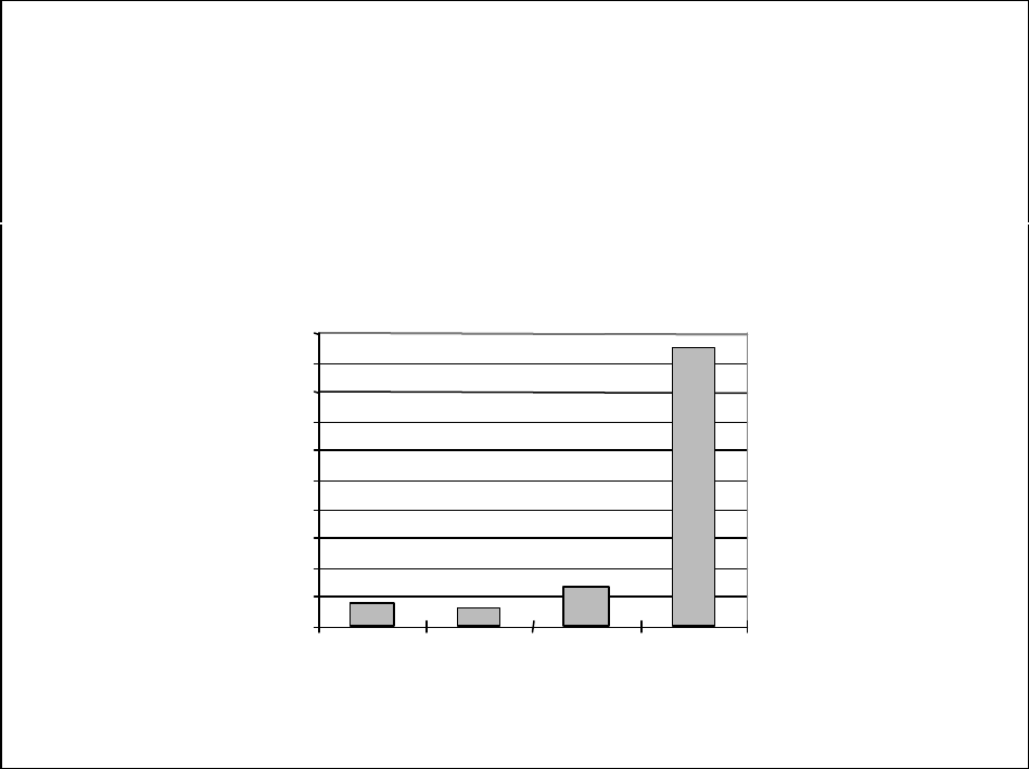
107
Example A11-3. Resistance to Ceratomyxa shasta. The infectious stage of the freshwater salmon
parasite C. shasta is found in some watersheds but not in others. Zinn et al. (1977) examined the
susceptibility of four fall chinook hatchery populations to C. shasta (see figure below). Three of
the populations originated from the Columbia River Basin, where the infectious stage of the
parasite is present, and the fourth originated from the Trask River, where the parasite is absent.
The three Columbia River populations all are resistant to the disease, whereas as the Trask River
population is highly susceptible. Resistance to the disease is believed to be genetically based
(e.g., Ibarra et al. 1994), and the selective mechanism is death due to the infectious agent.
0%
10%
20%
30%
40%
50%
60%
70%
80%
90%
100%
Big
Creek
Cowlitz
River
Oxbow
Trask
River
Figure A11-3a. Percent dead and infected with C. Shasta after 86 days of exposure. (From Zinn et al.
1977, Table 3.)
108
Selection
Selection refers to the differential fitness expressed by individuals exhibiting one version
of a trait in comparison to individuals exhibiting a different version of the trait. For example, if
salmon that return to spawn at a particular time are more successful than those that spawn earlier
or later, there is natural selection for the intermediate spawn time. Humans can also control
selection. For example, Donaldson (1968) discusses the use of artificial selection to breed for
desirable traits in chinook salmon and steelhead. If the variation has an appropriate genetic
basis, natural or artificial selection will alter the distribution of the trait being selected (reviewed
by Endler 1986, Falconer and Mackay 1996). Additionally, if multiple traits share some of the
same genes, selection pressures operating on one trait can cause correlated changes in other traits
(e.g., Lande and Arnold 1983).
Adaptation refers to the process by which natural selection increases a population's
fitness in its environment. Many natural salmonid populations appear to be highly adapted to
local environments (reviewed by Taylor 1991 and see examples in Box A11). However, these
adaptations can be threatened by human-caused selection for traits that are not adaptive in the
natural environment. For example, size is highly correlated with fecundity in salmonids
(reviewed by Groot and Margolis 1991). If large individuals in a population are harvested at
higher rates than smaller individuals, this can reduce the mean size of fish in a population and, as
a consequence, reduce fecundity as well (e.g., Ricker 1981). Box A12 provides several specific
examples of human-caused selection in salmonids that appear to cause either a loss of phenotypic
diversity or a loss of adaptation to the natural environment or both.
The time it takes for a population to adapt to a set of conditions varies among populations
and species. Several salmonid species are divided into subgroups that may have been relatively
isolated for many tens of thousands of years. Ocean and stream type chinook salmon in the
Columbia and Fraser Rivers, for example, have quite divergent life-history patterns (reviewed by
Healey 1991). Population genetic analysis suggests that these two life-history forms may have
diverged over 50,000 years ago (Myers et al. 1998, Ford 1998). Inland and coastal forms of
steelhead display similarly high levels of genetic divergence (Allendorf 1975, reviewed by
Busby et al. 1996). On the other hand, there is good evidence that salmon are capable of
recolonizing new habitat and adapting to new conditions very rapidly. For example, salmon
populations currently occupy large geographic areas that were inaccessible to salmon during the
last glacial advance ~14,000 years ago (reviewed by Pielou 1991), suggesting that at least over
long time scales salmon are flexible enough to adapt to new conditions. An apparent example of
much more rapid adaptation is the introduction of Sacramento River chinook salmon to New
Zealand early in the 20th century. Over the last nine decades, the originally introduced
population has not only naturally colonized additional rivers but has also become somewhat
diversified morphologically (Kinnison et al. 1998).
It is worth spending a moment to discuss natural selection and adaptation as they relate to
the NMFS's concept of an Evolutionarily Significant Unit (ESU—Waples 1991c). Evolution
embraces a continuum of concepts, ranging in meaning from small changes in allele frequencies
over a few generations to major changes in morphology over geological time scales (e.g.,
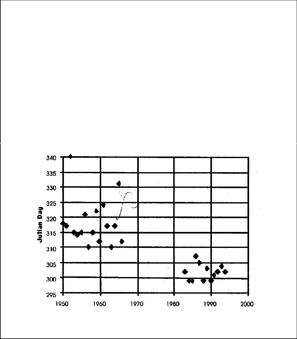
109
Box A12. Human caused selection.
Example A12-1. Spawn timing in Oregon coho. The spawn timing of some stocks of Oregon coast coho
salmon has shifted toward early dates over the last 45 years, apparently due to artificial and
natural selection in hatcheries (Nickelson et al. 1986). For example, Figure A12-1a shows the
mean spawn timing of Trask River Hatchery coho from 1950 to 1994. Nickelson et al. (1986)
compared the abundance of juvenile and adult coho salmon in 30 streams on the Oregon coast
from 1980 to 1985, 15 of which were supplemented with hatchery-produced presmolts from 1980
to 1982, and 15 of which were unsupplemented controls. The hatchery populations used for
supplementation included the Trask River (and other) Hatchery fish with advanced spawn timing.
The 15 supplemented streams showed increased total juvenile densities during the period of
stocking, but the adult densities were not significantly altered. In fact, the relative densities of
late spawning adults actually declined in the supplemented streams compared to the controls.
Nickelson et al. (1986) suggested the early spawn timing of the hatchery populations used for
supplementation was maladaptive in these streams because the fry from early spawners
experienced greater mortality from spring floods than later emerging fry (Figure A12-1b).
Although they did not rule out other possible factors such as poor survival of the hatchery fish
during other parts of their life cycle.
Figure A12-1a. Mean spawn timing of Trask Hatchery coho. (Data from Natural Resources Consultants
(1995).)
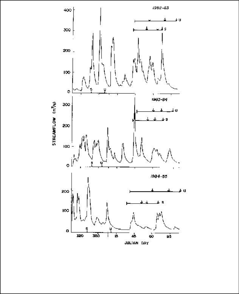
110
Figure A12-1b. Average daily streamflow for the Nestucca, Siletz, Yaquina, Alsea, and Siuslaw river
basins, November through April. The arrows on the horizontal axis designate the time at which
75% of the spawners had been observed in the stocked (S) and in the unstocked (U) study
streams. The estimated period from beginning until 75% emergence is shown by the horizontal
lines labeled S and U. The arrows represent the completion of 25, 50, and 75% of emergence.
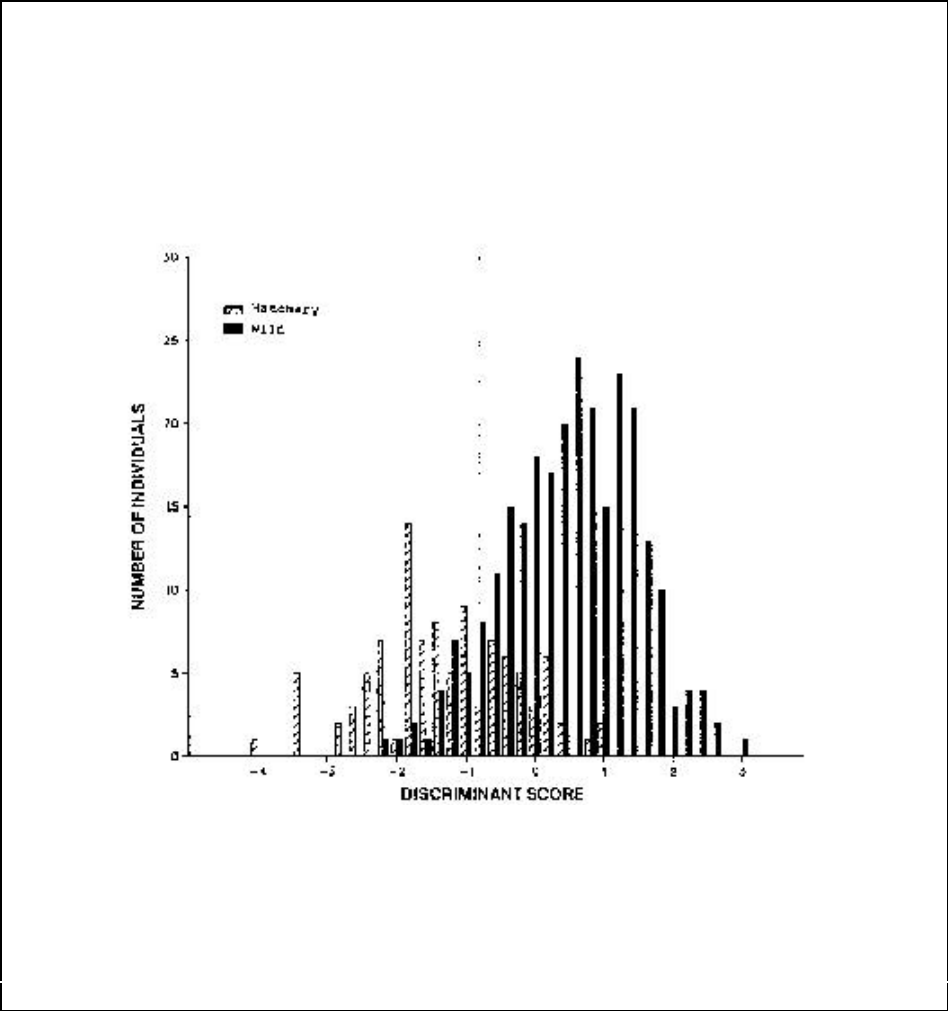
111
Example A12-2. Alteration of morphology and behavior in hatcheries. Fleming and Gross (1989)
compared the morphology of coho salmon from 13 wild and 5 hatchery populations, and found
that the hatchery populations differed from the wild populations in ways they predicted using
adaptationist arguments. For example, they predicted that the removal of female breeding
competition in hatcheries would relax selection for female secondary sex characteristics. Figure
A12-2a (reproduced from Fleming and Gross 1989) shows that this prediction was correct: traits
associated with breeding competition (size, kype development, and color) were significantly
changed in hatchery populations compared to wild populations.
Figure A12-2a. Discriminant scores of morphological variation between wild (N = 266) and hatchery (N
= 102) female coho salmon (Lorenzetta females excluded). The standardized canonical
discriminant function is: 0.488(kype) + 0.201(color) + 0.283(anal base) + 0.324(dorsal height) –
0.138(pelvic) + 0.171(pectoral) – 0.195(caudal peduncle) + 0.484(body length) (r = 0.622, P
2
<
0.001). The vertical line represents the point of discrimination between hatchery and wild fish
based upon the discriminant function. (Reproduced from Fleming and Gross (1989).)
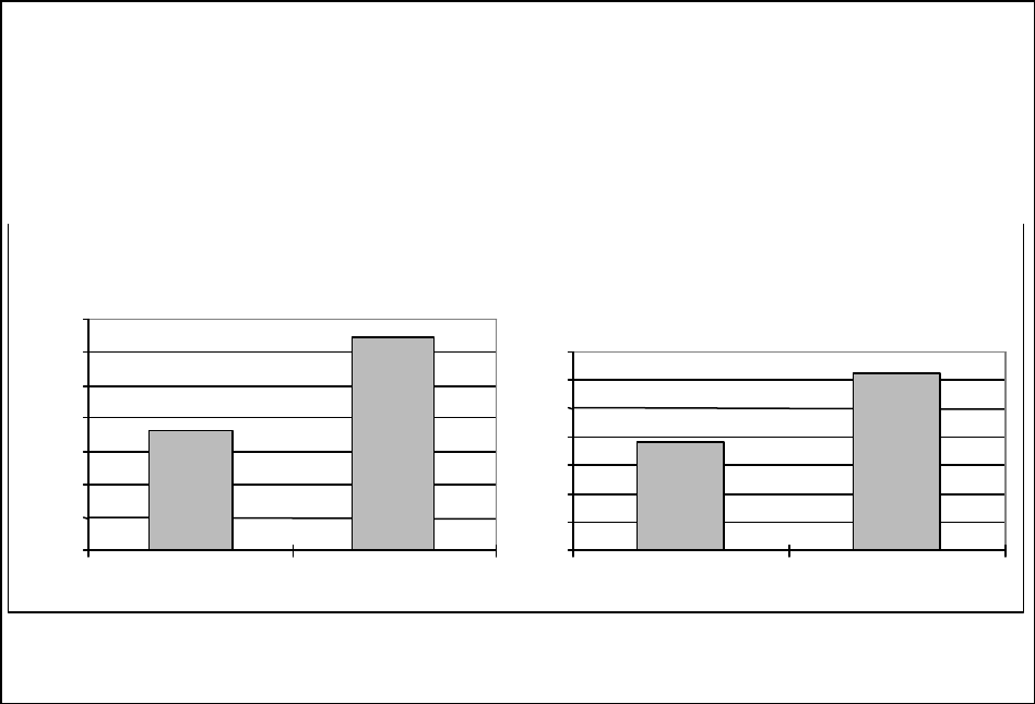
112
In another paper, the same authors compared breeding behavior and success in a common
environment between coho salmon from one hatchery population that had been in culture for 4-5
generations and 2 nearby wild populations. One of their findings was that the courting frequency
and breeding success of male coho salmon from the hatchery populations was significantly poorer
than that found in either wild population (Figure A12-2b). It is not clear from their results
whether the observed differences were the result of environmental or genetic differences between
the populations.
Courting frequency
0
0.05
0.1
0.15
0.2
0.25
0.3
0.35
hatchery wild
Breeding success (% of
surviving eggs fertilized)
0
1
2
3
4
5
6
7
hatchery wild
Figure A12-2b. (Data from Fleming and Gross 1993, Table 6.)
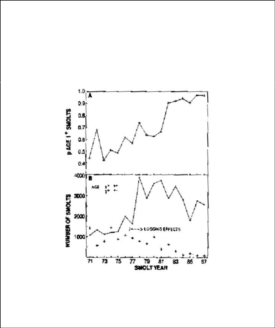
113
Example A12-3. Selection produced by habitat alteration. Many of the examples of local adaptation that
Taylor (1991) reviewed involve adaptation to the freshwater environment, so it is reasonable to
infer that altering this environment would affect patterns of phenotypic and genetic diversity (see
Healey and Prince 1995 for additional discussion). Hartman et al. (1984) and Holtby (1987)
provide an example of this from a 15-year study of the effects of logging on coho salmon in
Carnation Creek, British Columbia. One of the effects of logging was an increase in the water
temperature during incubation, which resulted in a large change in the relative proportions of one-
year-old and two-year-old smolts (Figure A12-3a, reproduced from Holtby 1987). From these
data, it is not possible to determine whether the observed change in phenotype is due to a plastic
response to a new environment, genetic change, or a combination of these factors.
Figure A12-3a. A) The proportion of smolts that were age 1+ by year of migration. B) The observed
numbers of yearling (1+) and two-year-old (2+) smolts by year of migration. Note that for any
particular cohort, the two-year-old smolts migrate one year after the yearlings. The change in the
age composition of smolts resulted from the dramatic increase in the numbers of the younger age
group (1+) rather than an abrupt decline in the numbers of older smolts. (Reproduced from
Holtby 1987.)
114
Kimura 1983, Endler 1986, Mayr 1988). The key to the NMFS's ESU concept is that
populations or groups of populations identified as ESUs are believed to have been on largely
independent evolutionary trajectories for many (probably at least hundreds) of generations, and
have therefore had an opportunity to become substantially genetically differentiated from other
ESUs. In other words, ESUs are populations or groups of populations that have been
reproductively isolated for a sufficient period of time such that they have accumulated a
substantial component of the diversity present in the entire biological species. Not all of the
differences among ESUs are necessarily adaptive or are the result of natural selection, but
adaptations are clearly an important factor in determining if two reproductively isolated
populations are in different ESUs (Waples 1991c).
Selection from human activities can potentially rapidly erode the adaptive fit between an
ESU or population and its environment, increasing the risk of extinction. We do not believe that
it is currently feasible to set quantitative guidelines on how much diversity a population or ESU
can loose and remain viable. Qualitatively, we suggest that in order for a population to be
considered viable, human-caused factors such as habitat changes, harvest pressures, artificial
propagation, or exotic species introductions should not substantially alter variation in the
population.
Straying and gene flow
Straying and gene flow strongly influence patterns of diversity within and among
populations. In this context, straying occurs when a fish returns to spawn in a population other
than its parents' population. Such strays may or may not successfully reproduce and leave
offspring. Gene flow refers to the movement of genes from one population to another, resulting
when strays successfully reproduce. The rate of gene flow is therefore influenced both by the
rate of straying among populations and by the level of selection against strays (see Felsenstein
1976, 1997 and Adkinson 1995 for recent theoretical treatments and reviews). For example,
Chilcote et al. (1986) and Leider et al. (1990) estimated that hatchery steelhead (introduced from
another tributary) that spawned naturally in the Kalama River, Washington, produced only about
one-tenth as many returning adults per spawner as the local wild fish, resulting in a gene flow
rate into the wild population that was much lower than would be predicted based on the observed
proportion of hatchery spawners. Information on stray rates comes primarily from experiments
that involve monitoring the spawning location of fish that are marked or tagged in their home
area as juveniles (e.g., Foerster 1936, Quinn and Fresh 1984, Quinn et al. 1991, Labelle 1992).
The rate of gene flow among populations, on the other hand, has usually been estimated by
fitting population genetic models to observed patterns of molecular genetic variation (reviewed
by Slatkin 1985). Gene flow and straying rates have only been estimated for the same groups of
populations a few times, and in each of these cases the rate of gene flow was estimated to be less
than the rate of straying (Quinn et al. 1987, Labelle 1992, Tallman and Healey 1994). The
methods used to estimate gene flow and straying in these studies were not precise enough, to
make accurate estimates of gene flow/stray rate ratios. For most species of Pacific salmonid,
straying and gene flow appear to occur in broadly hierarchical patterns, although the details of
these patterns vary considerably among species. For example, in a review of straying studies,
Quinn (1993) found that salmon stray with greater frequency to nearby populations than to
distant ones. Patterns of molecular genetic variation for most species fall into a similar pattern,
115
where geographically proximate populations are generally more genetically similar (and
therefore have higher estimated levels of gene flow) than geographically distant populations
(e.g., Utter et al. 1989, Ford 1998).
There are many theoretical population genetic models that can be used to interpret the
observed patterns of diversity among salmonid populations, and Box A13 provides examples of
two such models. The main conclusions from these (and similar) models are: 1) The level of
divergence among populations at selectively neutral alleles is a function of the number of
effective strays among populations. This is consistent with the empirical observation that both
straying and molecular genetic divergence appear to be generally correlated with geographic
proximity; 2) Selection can maintain genetic differences between populations in different
environments despite relatively high levels of gene flow between the populations. If selection is
sufficiently strong, a locally selected trait can be maintained at high frequency despite a large
influx of individuals exhibiting an alternative form of the trait (see Example 1 in Box A11); and
3) If a local environment selects against strays because of genetic factors at multiple loci, the rate
of recombination among these loci will affect the total strength of selection against strays
(Barton 1983). That is, the lower the rate of recombination, the more efficiently selection will
remove locally deleterious alleles. In salmonids, most traits likely to be involved in local
adaptation are quantitative traits that are probably controlled by many genes (reviewed by Hard
1995). Because salmon have a large number of chromosomes (reviewed by Sola et al. 1981), it
is probably reasonable to assume that levels of recombination among genes contributing to
quantitative traits will be high—making selection against strays potentially less effective than
might be the case in animals with fewer chromosomes.
There are a number of ways in which human actions can substantially alter patterns of
straying and, therefore, patterns of diversity and adaptation among salmonid populations. For
example, blocking migration corridors with dams and dewatering rivers can prevent salmonids
from homing and thus increase the rate of straying into other populations. Box A14 provides
several examples of how human actions have significantly altered straying patterns.
A reasonable way to approach setting VSP guidelines for acceptable levels of human-
caused gene flow among salmonid populations is to base the thresholds on estimates of naturally
occurring gene flow among natural salmon populations (Ryman et al. 1995). These natural rates
of gene flow allowed salmonid populations to persist and adapt to local conditions for many
generations, and it is therefore reasonable to assume that maintaining them would protect the
genetic diversity that currently exists among and within populations. Limiting human-caused
gene flow is particularly important when such gene flow occurs among different ESUs, because
ESUs are believed to contain adaptations that have been shaped by natural selection over the
course of hundreds of generations and to contain a substantial component of a species-genetic
diversity (Waples 1995). Loss of an ESU, either through extinction or through loss of its unique
genetic attributes, due to excess gene flow from outside the ESU, would therefore be a
significant, and probably irreplaceable, loss to the diversity of the species as a whole.
It is possible to estimate rates of gene flow among natural populations from patterns of molecular
genetic variation (see “Types of information used in identifying populations,” p. 39,
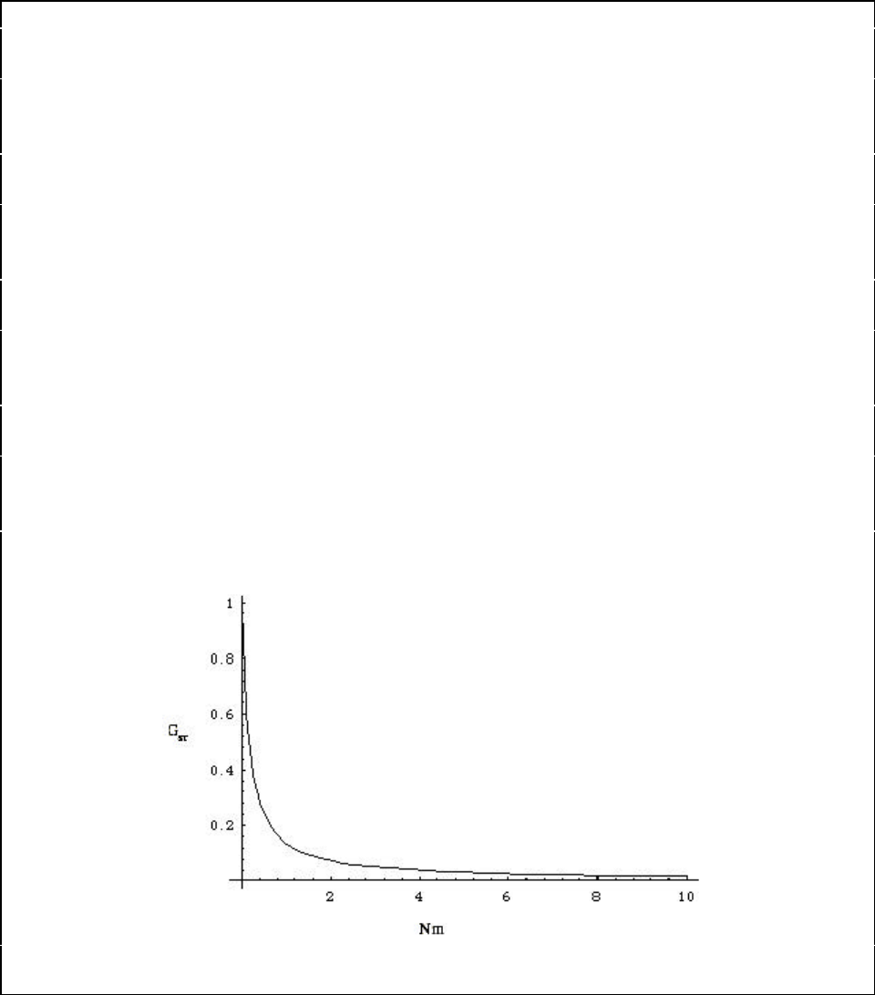
116
Box A13. Models of genetic variation among populations. There is a large body of literature on
modeling the effects of mutation, selection, drift, and migration on patterns of variation
among populations. In the following, we provide two examples of such models.
Example A13-1. Single locus, selectively neutral alleles, island model. Takahata and Nei (1984),
and Crow and Aoki (1984) explored a model of gene flow that assumed that a finite
number of populations were connected by equal rates of gene flow. G
ST
(a multi-allele
version of Wright's F
ST
) is a useful statistic for quantifying the relative amounts of
variation within and among populations, and varies from 0 (no variation among
populations) to 1 (all variation among populations). The approximate relationship
between G
ST
and the number of migrants per generation, Nm, at migration-drift
equilibrium is plotted in Fig A13-1a for five populations (the exact number of
populations does not substantially change the relationship). The figure shows that, in this
model, the level of population differentiation changes very rapidly with increasing gene
flow. For example, if the populations were previously at equilibrium between gene flow
and drift, and Nm is changed from 0.1 to 10, G
ST
for neutral alleles would be expected to
change from 0.6 to 0.02. When gene flow is increased from an old equilibrium level, the
time it takes G
ST
to approach its new equilibrium value is on the order of 1/m generations.
If the effective population sizes in the example above were 100, G
ST
would be near its
equilibrium value in about 10 generations. A similar relationship between G
ST
and Nm
holds for many non-island patterns of migration (e.g., Crow and Aoki 1984, Slatkin
1993).
Figure A13-1a. Approximate relationship between G
ST
and N
m
at equilibrium.

117
Example A13-2. Single locus models of selection and migration. Felsenstein (1976) extensively
reviewed general selection and migration models. As an illustration of the sorts of results
these models produce, we summarize the relatively simple model of Bulmer (1972). See
Adkison (1995) and Felsenstein (1997) for recent examples of how these concepts may
be applied to Pacific salmonids.
Bulmer's model was formulated for an arbitrary number of populations, but for the sake
of simplicity, we only present an example of the two-population case. For a single locus
with two alleles, A and a, let p
1
and p
2
be the frequencies of allele A in populations 1 and
2, respectively. Let the relative fitness of the genotypes AA, Aa and aa be 1 - s
1
, 1 and 1 -
t
1
, respectively in population 1, and 1 - s
2
, 1, and 1 - t
2,
respectively, in population 2. The
model assumes a life-cycle that consists of viability selection within each population,
migration among populations, and then random mating within each population The
recursion equations describing the change in the frequencies of the A allele in each
population are:
p
1
'
=
1 − m
1
(
)
p
1
2
1− s
1
(
)
+ p
1
q
1
(
)
1
−
t
1
q
1
2
−
s
1
p
1
2
+
m
1
p
2
2
1 − s
2
( )
+ p
2
q
2
( )
1
−
t
2
q
2
2
−
s
2
p
2
2
,
and
p
2
'
=
m
2
p
1
2
1
−
s
1
(
)
+
p
1
q
1
(
)
1− t
1
q
1
2
− s
1
p
1
2
+
1 − m
2
( )
p
2
2
1 − s
2
( )
+ p
2
q
2
( )
1− t
2
q
2
2
− s
2
p
2
2
,
Where m
1
is the proportion of population 1 that consists of migrants from population 2,
and m
2
is the proportion of population 2 that consists of migrants from population 1.
Although this model has not been fully solved analytically, it is easy to explore its
behavior iteratively using a computer. For example, running the model for 100
generations with parameters p
1
= 0.01, p
2
= 0.99, s
1
= t
2
= 0.1, s
2
= t
1
= -0.1, m
1
= 0.2 and
m
2
= 0.0 results in the elimination of the a allele in both populations (Figure A13-2a). In
other words, this scenario corresponds to a case where a locally favored allele is
eliminated by continual one-way gene flow from a different population that lacks the
allele. Even though the local allele is at a selective advantage compared to the migrant
allele, the local allele is eliminated from the population. Running the model with all the
same parameter values except m
1
= 0.05, results in the maintenance of the a allele in
population 1 (Figure A13-2a). In this case, the rate of migration of the alternative allele
was not high enough to completely overcome the selective advantage of the local allele.
This example illustrates how, under this model, a relatively small absolute difference in
the rate of gene flow can make a big difference in the patterns of diversity among
populations.
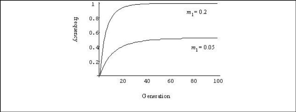
118
Figure A13-2a. Frequency of the A allele in population 1 with m
1
= 0.2 (top line) or m
1
= 0.05 (bottom
line).

119
Box A14. Examples of loss of diversity or adaptation due to human-caused gene flow alteration.
Example A14-1. Grand Coulee Dam. The construction of Grand Coulee Dam in 1939 blocked
anadromous fish from reaching over 1,800 river kilometers of the Columbia River Basin
(reviewed by Mullan et al. 1992). In order to mitigate this effect, all anadromous fish were
trapped at Rock Island Dam from 1939 to 1943 and were either released to spawn in tributaries
between Rock Island Dam and Grand Coulee Dam, or they spawned in hatcheries and their
offspring were released in this area (Mullan et al. 1992, Chapman et al. 1994). Although the
effects of this process on among-population diversity cannot be easily quantified (because pre-
dam data on population attributes are scant), it is likely that this random mixing of anadromous
salmonids from several major subbasins caused substantial diversity losses among the
populations.
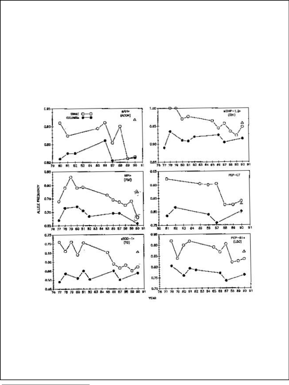
120
Example A14-2. Straying of Columbia River fall chinook into the Snake River. In their status review of
Snake River fall chinook salmon, Waples et al. (1991) illustrate the effects stray Columbia River
fall chinook have on allozyme allele frequencies in Snake River fall chinook. Figure A14-2a
shows temporal changes in allele frequencies of fall chinook in the Columbia River (wild fish
from the Hanford Reach and fish from Priest Rapids Hatchery) and Snake River (wild fish
sampled at Ice Harbor Dam and fish sampled at Lyons Ferry Hatchery). Strays from Columbia
River hatcheries (primarily fall chinook reared at Bonneville Hatchery and released in the
Umatilla River) first started appearing in the Snake River in significant numbers in the late 1980s,
and about the same time, allele frequencies in Snake River fall chinook converged toward the
allele frequencies of the Columbia River groups. (Note that the allele frequency plotted for Snake
River fall chinook at the PEP-LT locus in 1985 is incorrect. It is actually 0.875, rather than the
0.90 plotted in the figure [A. Marshall
12
].)
Figure A14-2a. Time series of allele frequency data at six gene loci for fall chinook salmon from the
Snake and upper Columbia Rivers, based on NMFS and WDF data summarized by Busack
(1991b, Table 10). Old locus names (as used by Utter et al. 1982) are shown in parentheses
below current names. Upper Columbia River data points are for wild samples from the Hanford
Reach area and samples from Pries Rapids Hatchery; unweighted averages were used in
combining multiple samples from the same year. Pre-1985 samples for the Snake River are for
presumably wild fish collected at Ice Harbor Dam; later samples are from Lyons Ferry Hatchery.
Two Lyons Ferry samples were analyzed in 1990; the open circle represents the sample of
returning CWT Lyons Ferry fish (primarily from the 1986 brood). (Reproduced from Waples et
al. 1991.)
12
Anne Marshall, WDFW, 600 Capital Way N., Olympia, WA 98501-1091. Pers. comm. April 2000.
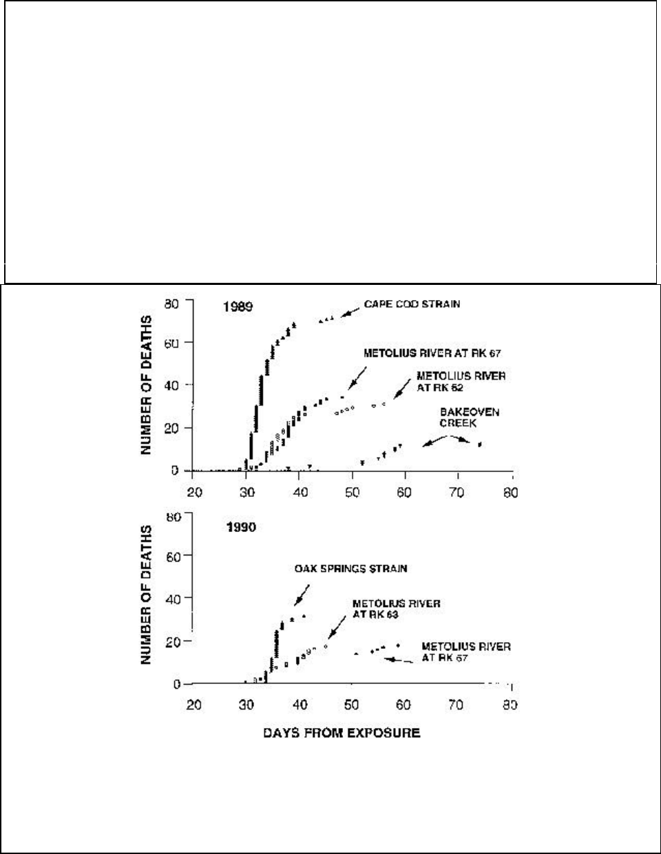
121
Example 14-3a. Loss of resistance to C. shasta in Metolius River rainbow trout. Differential resistance
to locally endemic pathogens is one type of local adaptation. Currens et al. (1997) provide an
example of how introgression of non-local genes can reduce the fitness of a locally-adapted
population. The freshwater parasite C. shasta is present in much of the Columbia River Basin,
but generally absent from coastal systems. Salmonid populations in the Columbia River Basin
are generally resistant to the parasite, whereas coastal populations are generally susceptible (see
Example A11-3). Currens et al. (1997) compared the resistance to C. shasta of a) native
Deschutes River rainbow trout and steelhead collected from areas with no history of hatchery
releases, b) hatchery rainbow trout from stocks originally derived from susceptible coastal
populations and planted in the Metolius River for many decades, and c) natural-origin Metolius
River rainbow trout. The Metolius River trout had allozyme allele frequencies and phenotypic
trait distributions that were intermediate between the native Deschutes River trout and the
coastal-origin hatchery stocks released into the Metolius River— indicating that Metolius River
trout populations had hybridized with the non-native hatchery stocks. The Metolius River
populations were also intermediate in susceptibility to C. shasta—indicating that gene flow from
these non-native populations has reduced the local populations’ resistance to this pathogen.
Figure A14-3a. Days to death by ceratomyxosis from initial exposure of rainbow trout to Ceratomyxa
shasta, 1989 and 1990. The Cape Cod and Oak Springs strains are coastal origin hatchery stocks
that were commonly planted in the Metolius River. The Metolius River fish are natural-origin
fish sampled from the Metolius River, and the Bakeoven Creek fish are native juvenile steelhead
sampled from Bakeoven Creek. (Reproduced from Currens et al. 1997.)
122
and references therein). This is the approach advocated by Ryman et al. (1995), who suggest
that acceptable rates of introgression be based on estimates of Nm, the number of genetically
effective migrants into a population per generation. Under an infinite island model of migration,
approximate values of Nm can be estimated from the relationship Nm = 1/(4F
ST
- 4) (see Box
A13 and discussion in “Types of information used in identifying populations,” p. 39). Rates of
gene flow among geographically diverse salmonid populations have been estimated using
population genetic survey data, and estimated levels of gene flow based on the genetic data are
generally very low. For example, Utter et al. (1989) surveyed variation among West Coast
chinook salmon at 25 polymorphic allozyme loci, and estimated F
ST
among major drainages
(roughly corresponding to the chinook salmon ESUs—Myers et al. 1998) to be 0.06. This
estimate of F
ST
results in an estimate of Nm of about four migrants per generation, which for
chinook salmon is about one migrant per year. Because these major drainages typically contain
thousands of spawners each generation, an estimate of four migrants per generation implies that
only a very small fraction of the genetically effective spawners in each major drainage are
migrants from other major drainages (e.g., if a major drainage contains N = 1,000 effective
spawners per generation, then m = ~0.4%). Similar levels among drainage genetic variation are
found for other species (e.g., steelhead, Reisenbichler et al. 1992; sockeye, Wood et al. 1994). In
addition, Johnson et al. (1999) recently used large unpublished NMFS and WDFW allozyme
data sets to estimate F
ST
among ESUs of five Pacific salmonid species—chum, coho, and
chinook salmon, and steelhead and cutthroat trout. Based on these F
ST
estimates, the average
number of migrants per generation between ESUs ranges from ~2.5 (chinook salmon) to ~13
(chum salmon). Based on these examples, the average proportion of an ESU that consists of
genetically effective migrants from other ESUs appears to be very small, certainly far less than
1%. We therefore conclude that if human factors (e.g., habitat degradation or hatcheries) cause
sustained rates of gene flow among ESUs to be greater than ~1%, this should definitely be cause
for concern. The choice of a 1% threshold is somewhat arbitrary and this guideline may in fact
be quite a bit higher than the natural rate of gene flow among many ESUs. We think a ~1%
guideline is reasonable, however, for two reasons. First, it seems likely that ESUs can sustain
rates of gene flow somewhat larger than they experienced historically and still remain viable.
Second, it seems unlikely that any guideline lower than ~1% could be effectively monitored.
Setting straying guidelines for populations within ESUs can be based on a similar approach, but
due to considerable variation among ESUs no single gene flow threshold is likely to apply within
all ESUs.
VSP Guidelines: Diversity
There is compelling evidence that patterns of phenotypic diversity within and among
Pacific salmonid populations are strongly influenced by the environments these populations
inhabit (reviewed by Ricker 1972, Taylor 1991, Healey and Prince 1995). There is less
compelling but still considerable evidence that much of this diversity is adaptive (reviewed by
Taylor 1991, see examples in Box A11) and that if it is lost or substantially altered population
viability would decrease. In fact, as the examples in Boxes A12 and A14 illustrate, human-
caused losses of diversity and adaptation have contributed to the poor status of some Pacific
Northwest salmonid populations. This suggests that in order to conserve the adaptive diversity
of salmonid populations, it is essential to: 1) conserve the environment to which they are adapted
(e.g., Healey and Prince 1995), 2) allow natural process of regeneration and disturbance to occur

123
Box A15. Diversity guidelines.
1. Human-caused factors such as habitat changes, harvest pressures, artificial propagation, and
exotic species introduction should not substantially alter variation in traits such as run timing,
age structure, size, fecundity, morphology, behavior, and molecular genetic characteristics.
Many of these traits may be adaptations to local conditions or they may help protect a population
against environmental variation. A mixture of genetic and environmental factors usually causes
phenotypic diversity, and this diversity should be maintained even if it cannot be shown to have a
genetic basis.
2. Natural processes of dispersal should be maintained. Human-cased factors should not
substantially alter the rate of gene flow among populations. Human caused inter-ESU stray rates
that are expected to produce (inferred) sustained gene flow rates greater than 1% (into a population)
should be cause for concern. Human caused intra-ESU stray rates that are expected to produce
substantial changes in patterns of gene flow should be avoided.
3. Natural processes that cause ecological variation should be maintained. Phenotypic diversity can
be maintained by spatial and temporal variation in habitat characteristics. This guideline involves
maintaining processes that promote ecological diversity, including natural habitat disturbance regimes
and factors that maintain habitat patches of sufficient quality for successful colonization.
4. Population status evaluations should take uncertainty about requisite levels of diversity into
account. Our understanding of the role diversity plays in Pacific salmonid viability is limited.
Historically, salmonid populations were generally self-sustaining, and the historical representation of
phenotypic diversity serves as a useful “default” goal in maintaining viable populations.
124
(e.g., Reeves et al. 1995), and 3) limit or remove human-caused selection or straying that
weakens the adaptive fit between a salmonid population and its environment or limits a
population's ability to respond to natural selection (e.g., Ryman et al. 1995).
Viable ESUs
Three factors need to be considered when relating VSPs to viable ESUs: 1) Catastrophic
events, 2) long-term demographic processes, and 3) long-term evolutionary potential. In this
section we describe the effect each of these factors has with respect to viability and we lay out
guidelines for evaluating ESU viability.
Catastrophes
A catastrophe is a sudden event that severely reduces or eliminates an entire population.
For the purposes of this discussion “severe” reductions involve elimination of more than 75% of
the breeding adults, though we acknowledge that this is a somewhat arbitrary threshold that may
be modified to reflect the dynamics of a particular population or ESU. By “sudden,” we mean
events that happen within a single season, though the impact may not be observed until several
seasons later. Events that unfold over a longer time span are discussed in the sections on long-
term demographics and evolution. It should be noted that environmental events form a
continuum from catastrophes to the “normal” environmental variation considered in VSP
analysis.
Historically, natural catastrophes that affect entire populations were probably rare events
at the 100-year time scale (Bisson et al. 1997). However, human activity may have increased the
frequency of some types of catastrophe. We considered the effects of catastrophes at the ESU
level rather than at the individual population level for three reasons: 1) because they have the
potential to affect large as well as small populations, catastrophes can differ qualitatively from
the stochastic processes considered in VSP evaluations, 2) concerns about catastrophic risk may
extend beyond the 100-year time scale used to evaluate VSPs, and 3) catastrophic events can
affect more than one population at a time, making it appropriate to evaluate catastrophic risk at
the ESU-level. Although we are discussing catastrophes at the level of the ESU, it will generally
be necessary to evaluate the catastrophic risk in terms of individual populations, and then
integrate this information in an overall assessment of ESU status. Catastrophic events may be of
natural or anthropogenic origin or a combination of the two. Natural catastrophes include
volcanoes, earthquakes, disease epidemics, extreme weather, landslides, and unusual fires.
Anthropogenic catastrophes include oil and chemical spills, dam construction, water
diversion/dam failures, and major miscalculations in harvest plans. Catastrophes may also result
from the interaction of natural and anthropogenic effects. For example, a rainstorm that would
have little affect on a salmonid population under pristine conditions could become a catastrophe
in a heavily modified landscape that has been clear-cut or intensively urbanized. Thus, human
activities can increase the frequency of some types of catastrophic events. Bisson et al. (1997)
list different types of natural and anthropogenic disturbances that affect salmon populations and
attempt to estimate the frequency of each.
125
Catastrophes can profoundly affect extinction risk. In fact, models predict that the rate
and severity of catastrophes can be the most important factor in determining a population’s
extinction risk (Menges 1990, Lande 1993, Mangel and Tier 1994). For example, the recovery
plan for the federally-listed southern sea otter in California identified catastrophic oil spills as the
primary risk to population viability. Recovery goals were based on quantitative estimates of the
risks associated with this type of catastrophe (Ralls et. al. 1996). Given the number of potential
catastrophic threats facing salmonid populations, in many situations we would expect
catastrophes to have a substantial influence on extinction risk. Thus, most of the guidelines
regarding ESU viability focus on catastrophic risk.
If estimates of the per-population rate of catastrophic events can be obtained, it may be
possible to get an estimate of the extinction risk posed by catastrophes to the entire ESU.
Reliability theory is a branch of probability modeling that is used by engineers to predict the rate
of device failure as a function of the rate of failure of the individual components in the device
(Barlow and Proschan 1975, Leemis 1995, Wolstenholme 1999). Populations may be considered
as “components” in the “device” that is the ESU (Ruckelshaus et. al, 2000). Using reliability
theory, scenarios involving different combinations of populations can be explored to test
hypotheses about ESU viability. In a simple scenario, for example, ESU extinction risk from
catastrophes may be estimated after assuming that five populations are necessary for ESU
persistence and all five populations have the same risk of catastrophic extinction. This can be
compared to a scenario in which only two populations are assumed necessary. Using the tools of
reliability theory, it is possible to explore quite complicated scenarios in which populations have
different catastrophic risks of failure, certain populations or “types” of populations are
considered a priori to be essential for viability and in which population recovery is possible. The
major obstacle in the application of reliability theory is obtaining accurate estimates of
catastrophe rates.
Long-term Demographic and Evolutionary Processes
The VSP guidelines focus on processes that occur at temporal scales of 100 years or less.
However, an ESU’s long-term viability also depends on population extinction and recolonization
processes that occur over longer time scales. Because catastrophic events are certain to occur at
one point or another, we expect populations or groups of salmonid populations occasionally to
become extinct from natural causes. In addition to catastrophic events, gradual, but significant
climatic shifts can lead to population extinction, as can habitat changes arising from ecological
succession or changes in environmental conditions. After a catastrophic event or climate shift
we expect a new configuration of populations to arise within an ESU as some populations are
lost and new populations are established. All of these large-scale changes in ESU structure may
be accompanied by changes in evolutionary dynamics and genetic characteristics.
Although long-term (>100 year) demographic and evolutionary processes unarguably
operate in salmonid ESUs, it is difficult to make credible quantitative predictions about ESU
viability over long time spans. There is a general recognition that among-population genetic and
phenotypic diversity is important to persistence and that the spatial distribution of diversity
influences long-term dynamics, but it is difficult to generalize beyond these simple statements.

126
Therefore, perhaps the best recommendation with regard to long-term processes is ESU Viability
Guideline 7, which recommends that when in doubt, we should strive to maintain historic
population numbers and distributions.
ESU Viability Guidelines
Box A16. ESU viability guidelines.
1. ESUs should contain multiple populations. If an ESU is made up of multiple populations, it is less
likely that a single catastrophic event will cause it to become extinct. Also, ESUs may function as
“metapopulations” over the long term and the existence of multiple populations would be necessary
for the operation of sustainable population-level extinction/recolonization processes. In addition,
multiple populations within an ESU increase the likelihood that a diversity of phenotypic and
genotypic characteristics will be maintained, thus allowing natural evolutionary processes to operate
and increasing the ESU’s viability in the long term. Obviously, this guideline does not apply to ESUs
that appear to contain a single population (e.g., Lake Ozette sockeye). In ESUs containing a single
population, Guideline 6 becomes increasingly important.
2. Some populations in an ESU should be geographically widespread. Spatially correlated
environmental catastrophes are less likely to drive a widespread ESU to extinction. This guideline
also directly relates to the ESA mandate of protecting a species in a “significant portion of (its)
range.”
3. Some populations should be geographically close to each other. On long temporal scales, ESUs
may function as “metapopulations” and having populations geographically close to one another
facilitates connectivity among existing populations. Thus, a viable ESU requires both widespread
(Guideline 2) AND spatially close populations.
4. Populations should not all share common catastrophic risks. An ESU containing populations that
do not share common catastrophic risks is less likely to be driven to extinction by correlated
environmental catastrophes. Maintaining geographically widespread populations is one way to
reduce risk associated with correlated catastrophes (Guideline 2), but spatial proximity is not the only
reason why two populations could experience a correlated catastrophic risk.
5. Populations that display diverse life-histories and phenotypes should be maintained. When an
ESU’s populations hava fair degree of life-history diversity (or other phenotypic diversity), the ESU
is less likely to go extinct as a result of correlated environmental catastrophes or changes in
environmental conditions that occur too rapidly for an evolutionary response. In addition—assuming
phenotypic diversity is caused at least in part by genetic diversity—maintaining diversity allows
natural evolutionary processes to operate within an ESU.
6. Some populations should exceed VSP guidelines. Larger and more productive (“resilient”)
populations may be able to recover from a catastrophic event that would cause the extinction of a
smaller population. An ESU that contains some populations in excess of VSP threshold criteria for
abundance and population growth rate is less likely to go extinct in response to a single catastrophic
event that affects all populations. It is important to note that the abundance guidelines do not take
catastrophes into account. This guideline is particularly relevant if an ESU consists of a single
population.
7. Evaluations of ESU status should take into account uncertainty about ESU-level processes. Our
understanding of ESU-level spatial and temporal process is very limited. ESUs are believed to have
been historically self-sustaining and the historical number and distribution of populations serve as a
useful “default” goal in maintaining viable ESUs.
127
LITERATURE CITED
Adkison, M. D. 1995. Population differentiation in Pacific salmon: Local adaptation, genetic
drift, or the environment? Can. J. Fish. Aquat. Sci. 52: 2762-2777.
Allendorf, F. W. 1975. Genetic variability in a species possessing extensive gene duplication:
Genetic interpretation of duplicate loci and examination of genetic variation in populations of
rainbow trout. Ph.D. Thesis. University of Washington, Seattle, WA, 98 p.
Allendorf, F. W., and G. H. Thorgaard. 1984. Tetraploidy and the evolution of salmonid fishes.
In B. J. Turner (ed.), Evol. Genet. Fish. p. 1-53. Plenum Press, New York.
Allendorf, F. W., D. Bayles, D. L. Bottom, K. P. Currens, C. A. Frissell, D. Hankin, J. A.
Lichatowich, W. Nehlsen, P. C. Trotter, and T. H. Williams. 1997. Prioritizing Pacific
salmon stocks for conservation. Conserv. Biol. 11: 140-152.
Barker, R. J., and J. R. Sauer. 1992. Modeling population change from time series data. In D.
R. McCullough and R. Barrett (eds.), Wildlife 2001: Populations, p.182-194. Elsevier,
New York.
Barlow, R. E., and F. Proschan. 1975. Statistical theory of reliability and life testing probability
models. Holt, Rinehart and Winston, New York, 290 p.
Barnhart, R. A. 1986. Species profiles: Life histories and environmental requirements of coastal
fishes and invertebrates (Pacific Southwest)—steelhead. U.S. Fish Wild. Serv. Biol. Rep.
82: 11-60.
Barnhart, R. A. 1995. Salmon and steelhead populations of the Klamath-Trinity Basin,
California. In T. J. Hassler (ed.), Klamath Basin Fisheries Symposium, p. 73-97.
California Cooperative Fishery Unit. Humboldt State University, Arcata, CA.
Barrowclough, G. 1980. Gene flow, effective population sizes, and genetic variance
components in birds. Evolution 34: 789-798.
Bartley, D., M. Bagley, G. Gall, and B. Bentley. 1992. Use of linkage disequilibrium data to
estimate effective size of hatchery and natural fish populations. Conserv. Biol. 6: 365-375.
Barton, N. H. 1983. Multilocus clines. Evolution 37: 454-471.
Bascompte, J., and R. V. Sole. 1996. Habitat fragmentation and extinction thresholds in
spatially explicit models. J. Anim. Ecol. 65: 465-473.
Beacham, T. D., and T. P. T. Evelyn. 1992. Genetic variation in disease resistance and growth
of chinook, coho, and chum salmon with respect to vibriosis, furunculosis, and bacterial
kidney disease. Tran. Am. Fish. Soc. 121: 456-485.
128
Beamish, R. J., and D. R. Bouillon. 1993. Pacific salmon production trends in relation to
climate. Can. J. Fish. Aquat. Sci. 50: 1002-1016.
Beamish, R. J., C. Mahnken, and L. M. Neville. 1997. Hatchery and wild production of Pacific
salmon in relation to large-scale, natural shifts in productivity of the marine environment.
ICES J. Mar. Sci. 54: 1200-1215.
Beamish, R. J., D. J. Noakes, G. A. MacFarlane, L. Klyshatorin, V. V. Ivanov, and V. Kurashov.
1999. The regime concept and natural trends in the production of Pacific salmon. Can. J.
Fish. Aquat. Sci. 56: 516-526.
Belovsky, G. E. 1987. Extinction models and mammalian persistence. In M. E. Soulé (ed.),
Viable populations for conservation, p. 35-57. Cambridge University Press, Cambridge,
MA.
Bence, J. R. 1995. Analysis of short time series: correcting for autocorrelation. Ecology 76:
628-639.
Benda, L. E. 1994. Stochastic geomorphology in a humid mountain landscape. Ph.D. Thesis.
University of Washington, Seattle, WA, 356 p.
Berryman, D., B. Bobee, D. Cluis, and J. Haemmerli. 1988. Nonparametric tests for trend
detection in water quality time series. Water Resour. Bull. 24: 545-556.
Beverton, R. J. H., and S. J. Holt. 1957. On the dynamics of exploited fish populations. Minist.
Agric. Fish. (UK), London, 533 p.
Bigler, B. S., D. W. Welch, and J. H. Helle. 1996. A review of size trends among North Pacific
salmon (Oncorhynchus spp.). Can. J. Fish. Aquat. Sci. 53: 455-465.
Bilby, R. E., B. R. Fransen, and P. A. Bisson. 1996. Incorporation of nitrogen and carbon from
spawning coho salmon into the trophic system of small streams: Evidence from stable
isotopes. Can. J. Fish. Aquat. Sci. 53: 164-173.
Bilby, R. E., B. R. Fransen, P. A. Bisson, and J. K. Walter. 1998. Response of juvenile coho
salmon (Oncorhynchus kisutch) and steelhead (Oncorhynchus mykiss) to the addition of
salmon carcasses to two streams in southwestern Washington, USA. Can. J. Fish. Aquat.
Sci. 55: 1909-1918.
Bilby, B. E., G. R. Pess, B. Feist, and T. J. Beechie. 1999. Freshwater Habitat and Salmon
Recovery: Relating Land Use Actions to Fish Population Response. Proceedings of the
Fish Habitat Workshop, National Marine Fisheries Service. Seattle, WA, 28 p.
129
Bisson, P. A., G. H. Reeves, R. E. Bilby, and R. J. Naiman. 1997. Watershed management and
Pacific salmon: Desired future conditions. In D. J. Stouder, P. A. Bisson, and R. J.
Naiman (eds.), Pacific salmon and their ecosystems, p. 447-474. Chapman and Hall,
New York.
Bjorkstedt, E. P., unpubl. data. National Marine Fishery Service, southwest Fishery Science
Center, 3150, Paradise Dr., Tiboron, CA 94920-1205.
Bjorkstedt, E. P. 2000. Stock-recruitment relationships for life cycles that exhibit concurrent
density dependence. Can. J. Fish. Aquat. Sci. 54: 459-467.
Botsford, L. W., and J. G. Brittnacher. 1998. Viability of Sacramento winter-run chinook
salmon. Conserv. Biol. 12: 65-79.
Bouzat, J. L., H. H. Cheng, H. A. Lewin, R. L. Westemeier, J. D. Brown, and K. N. Paige.
1998a. Genetic evaluation of a demographic bottleneck in the Greater Prairie Chicken.
Conserv. Biol 12: 836-843.
Bouzat, J. L., H. A. Lewin, and K. N. Paige. 1998b. The ghost of genetic diversity past:
Historical DNA analysis of the greater prairie chicken. Am. Nat. 152: 1-6.
Box, G. E. P., G. C. Tiao. 1975. Intervention analysis with applications to economic and
environment problems. J. Am. Stat. Assoc. 70: 70-79.
Bradford, M. J. 1995. Comparative review of Pacific salmon survival rates. Can. J. Fish.
Aquat. Sci. 52: 1327-1338.
Bradford, M. J. 1999. Temporal and spatial trends in the abundance of coho salmon smolts
from Western North America. Trans. Am. Fish. Soc. 128: 840-846.
Bradford, M. J., G. C. Taylor, and J. A. Allan. 1997. Empirical review of coho salmon smolt
abundance and prediction of smolt production at the regional level. Trans. Am. Fish.
Soc. 126: 49-64.
Brawn, J. D., and S. K. Robinson. 1996. Source-sink population dynamics may complicate the
interpretation of long-term census data. Ecology 77: 3-12.
Brown, L. G. 1995. Mid-Columbia River summer steelhead stock assessment: A summary of
the Priest Rapids steelhead sampling project 1986-1994 cycles. WA. Dep. Fish Wild.
Progress Report Number AF95-02, 85 p.
Bryant, E. H., and M. Meffert. 1990. The effects of bottlenecks on genetic variation, fitness and
quantitative traits in the housefly. In E. C. Dudley (ed.), Fourth International Congress of
Systematic and Evolutionary Biology, p. 591-601. Dioscordies Press, Portland, OR.
Bulmer, M. G. 1972. Multiple niche polymorphism. Am. Nat. 106: 254-257.
130
Burger, R., and M. Lynch. 1995. Evolution and extinction in a changing environment: A
quantitative-genetic analysis. Evolution. 49: 151-163.
Burgman, M. A., S. Ferson, and H. R. Akcakaya. 1993. Risk assessment in conservation
biology. Chapman and Hall, New York, 314 p.
Burgner, R. L. 1991. Life history of sockeye salmon Oncorhynchus nerka. In C. Groot and L.
Margolis (eds.), Pacific salmon life histories, p. 3-117. University of British Columbia
Press, Vancouver, B. C.
Busby, P. J., T. C. Wainwright, G. J. Bryant, L. J. Lierheimer, R. S. Waples, F. W. Waknitz, and
I. V. Lagomarsino. 1996. Status review of West Coast steelhead from Washington,
Idaho, Oregon, and California. NOAA Tech. Memo. NMFS-NWFSC-27, 261 p.
Busby, P. J., T. C. Wainwright, and R. S. Waples. 1994. Status review for Klamath Mountains
Province steelhead. NOAA Tech. Memo. NMFS-NWFSC-19, 130 p.
Caballero, A. 1994. Developments in the prediction of effective population size. Heredity
73: 657-679.
California Department of Fish and Game (CDFG). 1998. Report to the Fish and Game
Commission: a status review of the spring-run chinook salmon (Oncorhynchus
tshawytscha) in the Sacramento River drainage. California Department of Fish and
Game Candidate Species Status Report 98-01.
Caswell, H. 1989. Matrix Population Models: Construction, Analysis, and Interpretation.
Sinauer, Associates, Sunderland, MA, 328 p.
Caughley, G. 1994. Directions in conservation biology. J. Anim. Ecol. 63: 215-244.
Caughley, G., and A. Gunn. 1996. Conservation biology in theory and practice. Blackwell
Science, Cambridge, MA, 459 p.
Chapman, D., C. Pevan, T. Hillman, A. Giorgi, and F. Utter. 1994. Status of summer steelhead
in the mid-Columbia River. Don Chapman Consultants Inc., Boise, ID, 235 p.
Chilcote, M. W., S. A. Leider, and J. J. Loch. 1986. Differential reproductive success of
hatchery and wild summer-run steelhead under natural conditions. Trans. Am Fish Soc.
115: 726-735.
Clarke, W. C., R. E. Withler, and J. E. Shelbourn. 1992. Genetic control of juvenile life history
pattern in chinook salmon (Oncorhynchus tshawytscha). Can J. Fish. Aquat. Sci.
49: 2300-2306.
131
Connor, R. N. 1988. Wildlife populations: Minimally viable or ecologically functional? Wildl.
Soc. Bull. 16: 80-84.
Cooper, A. B., and M. Mangel. 1999 . The dangers of ignoring metapopulation structure for the
conservation of salmonids. Fish. Bull. 97: 213-226.
Courchamp, F., T. Clutton-Brock, and B. Grenfell. 1999. Inverse density-dependence and the
Alee effect. Trends Ecol. Evol. 14: 405-410.
Craig, J. K. 1995. Genetic divergence in spawning color of sympatric forms of sockeye salmon
(Oncorhynchus nerka): Investigation of an unknown form. Master's Thesis. University
of Washington, Seattle, WA, 105 p.
Cramer, S. P. 1989. Contribution of Sacramento Basin hatcheries to ocean catch and river
escapement of fall chinook salmon. S. P. Cramer and Associates, Inc., Gresham, OR, 113 p.
Crawford, T. J. 1984. What is a population? In B. Shorrocks (ed.), Evolutionary Ecology,
p. 135-173. Blackwell International, Oxford.
Crow, J., and K. Aoki. 1984. Group selection for a polygenic behavioral trait: estimating the
degree of population subdivision. Proc. Nat. Acad. Sci. (USA) 81: 6073-6077.
Crow, J. F., and M. Kimura. 1970. An introduction to populations genetics theory. Harper &
Row, New York, 591 p.
Currens, K. P., S. L. Stone, and C. B. Schreck. 1987. A genetic comparison of rainbow trout
(Salmo gairdneri) above and below Izee Falls in the John Day River, Oregon. Genetics
Lab Report (87) 2. Oregon Cooperative Fisheries Research Unit, Department of
Fisheries and Wildlife, Oregon State University. Corvallis, OR, 34 p.
Currens, K., J. Lannan, B. Riddell, D. Tave, and C. Wood. 1996. U.S. v. Oregon dispute
resolution. Responses of the independent scientific panel to questions about the
interpretation of genetic data for spring chinook salmon in the Grand Ronde Basin. Draft
Report, 43 p.
Currens, K. P., A. R. Hemmingsen, R. A. French, D. V. Buchanan, C. B. Schreck, and W. L.
Hiram. 1997. Introgression and susceptibility to disease in a wild population of rainbow
trout. N. Am. J. Fish. Manage. 17: 1065-1078.
Currens, K. P., F. W. Allendorf, D. Bayles, D. L. Bottom, C. A. Frissell, D. Hankin, J. A.
Lichatowich, P. C. Trotter, and T. A. Williams. 1998. Conservation of Pacific salmon:
Response to Wainwright and Waples. Conserv. Biol. 12: 1148-1149.
Cushing, J. M. 1996. Nonlinear Matrix Equations and Population Dynamics. In S. Tuljapurkar
and H. Caswell (eds.), Structured-population models in marine, terrestrial, and freshwater
systems, p. 205-243. Chapman & Hall.
132
Day, J. R., and H. P. Possingham. 1995. A stochastic metapopulation model with variability in
patch size and position. Theor. Popul. Biol. 48: 333-360.
Dempson, J. B., and D. E. Stansbury. 1991 . Using partial counting fences and a two-sample
stratified design for mark-recapture estimation of an Atlantic salmon smolt population.
N. Am. J. Fish. Manage. 11.
Dennis, B. 1989. Allee effects: Population growth, critical density, and the chance of extinction.
Natural Resource Modeling 3: 481-538.
Dennis, B., W. P. Kemp, and M. L. Taper. 1998. Joint density dependence. Ecology
79: 426-441.
Dennis, B., P. L. Munholland, and J. M. Scott. 1991. Estimation of growth and extinction
parameters for endangered species. Ecol. Monogr. 61: 115-143.
Dennis, B., and M. L. Taper. 1994. Density dependence in time series observations of natural
populations: Estimation and testing. Ecol. Monogr. 64: 205-224.
DeVries, P. 1997. Riverine salmonid egg burial depths: review of published data and
implications for scour studies. Can. J. Fish. Aquat. Sci. 54: 1685-1698.
Donaldson, L. R. 1968. Selective breeding of salmonids fishes. In W. J. McNeil (ed.), Marine
Aquaculture. Selected papers from the conference on marine aquaculture, p. 65-74.
Oregon State University Press, Corvallis, OR.
Dunham, J. B., and B. E. Rieman. 1999. Metapopulation structure of bull trout: influences of
physical biotic and geometrical landscape characteristics. Ecol. Apps. 9: 642-655.
Ehrlich, P. R., and J. R. Roughgarden. 1987. The Science of Ecology. MacMillian Publishing
Company, New York, 710 p.
Emlen, J. M. 1995. Population viability of the Snake River chinook salmon (Oncorhynchus
tshawytscha). Can. J. Fish. Aquat. Sci. 52: 1442-1448.
Endler, J. A. 1986. Natural Selection in the Wild. Princeton University Press, Princeton, NJ,
337 p.
English, K. K., R. C. Bocking, and J. C. Irvine. 1992. A robust procedure for estimating salmon
escapement based on the area-under-the-curve method. Can. J. Fish. Aquat. Sci.
49: 1982-1989.
Fagan, W. F., E. Meir, and J. L. Moore. In press. Variation thresholds for extinction and their
implications for conservation strategies. Am. Nat.
133
Fahrig, L., and G. Merriam. 1994. Conservation of fragmented populations. Conserv. Biol.
8: 50-59.
Falconer, D. S. 1981. Introduction to Quantitative Genetics. Longman Group Ltd., Essex,
England, 340 p.
Falconer, D. S., and T. F. C. Mackay. 1996 . Introduction to Quantitative Genetics. Longman
Group Ltd., Essex, England, 464 p.
Felsenstein, J. 1976. The theoretical population genetics of variable selection and migration.
Annu. Rev. Genet. 10: 253-280.
Felsenstein, J. 1997. Population differentiation and evolutionary processes. In W. S. Grant
(ed.), Genetic effects of straying of non-native hatchery fish into natural populations, p.
31-43. NOAA Tech. Memo. NMFS-NWFSC-30.
Fleming, I. A., and M. R. Gross. 1993. Breeding success of hatchery and wild coho salmon
(Onchorhynchus kisutch) in competition. Ecol. Apps. 3: 230-245.
Fleming, I. A., and M. R. Gross. 1989. Evolution of adult female life history and morphology in
a Pacific salmon (coho: Oncorhynchus kisutch ). Evolution 43: 141-157.
Foerster, R. E. 1936. The return from the sea of sockeye salmon (Oncorhynchus nerka) with
special reference to percentage survival, sex proportions and progress of migration.
J. Biol. Board Can. 3: 26-42.
Foerster, R. E. 1968. The sockeye salmon, Oncorhynchus nerka. Bull. Fish. Res. Board Can.
162: 422.
Foley, P. 1994. Predicting extinction times from environmental stochasticity and carrying
capacity. Conserv. Biol. 8: 124-137.
Foley, P. 1997. Extinction models for local populations. In I. A. Hanski and M. E. Gilpin
(eds.), Metapopulation biology: ecology genetics and evolution, p. 215-246. Academic
Press, San Diego, CA.
Foote, C. J., C. C. Wood, and R. E. Withler. 1989. Biochemical genetic comparison of sockeye
salmon and kokanee, the anadromous and nonanadromous forms of Oncorhynchus nerka.
Can. J. Fish. Aquat. Sci. 46: 149-158.
Ford, M. J. 1998. Testing models of migration and isolation among populations of chinook
salmon (Oncorhynchus tschawytscha). Evolution 52: 539-557.
134
Ford, M., P. Budy, C. Busack, D. Chapman, T. Cooney, T. Fisher, J. Geiselman, T. Hillman, J.
Lukas, C. Peven, C. Toole, E. Weber, and P. Wilson. 1999a. Upper Columbia River
steelhead and spring chinook salmon population structure and biological requirements.
Draft report prepared by the Upper Columbia River Steelhead and Spring Chinook
Salmon Biological Requirements Committee, dated 14 December 1999. National Marine
Fisheries Service, Northwest Fisheries Science Center.
Ford, M. J., P. J. Thornton, and L. K. Park. 1999b. Natural selection promotes divergence of
transferrin among salmonid species. Mol. Ecol. 8: 1055-1061.
Frankham, R. 1995. Effective population size/adult population size ratios in wildlife: A review.
Genet. Resour. 66: 95-107.
Frankham, R. 1998. Inbreeding and extinction: Island population. Conserv. Biol. 12: 665-675.
Franklin, I. R. 1980. Evolutionary change in small populations. In M. E. Soulé and B. A.
Wilcox (eds.), Conservation Biology, An Evolutionary-Ecological Perspective,
p. 135-149. Sinauer Associates, Sunderland, MA.
Gabriel, W., and R. Bürger. 1992. Survival of small populations under demographic
stochasticity. Theor. Popul. Biol. 41: 44-71.
Garcia, T. 1998. Letter from Terry Garcia (Assistant Secretary for Oceans and Atmosphere
Department of Commerce) to Ted Strong (Executive Director of the Columbia River
Inter-Tribal Fish Commission) re: federal trust responsibility to the four Columbia River
Treaty Tribes and the Endangered Species Act, dated 21 June 1998. 2 p. U.S.
Department of Commerce, Assistant Secretary for Oceans and Atmosphere, Washington
D.C., 20230.
Geiger, H. J., W. W. Smoker, L. A. Zhivotovsky, and A. J. Gharrett. 1997. Variability of family
size and marine survival in pink salmon (Oncorhynchus gorbuscha) has implications for
conservation biology and human use. Can. J. Fish. Aquat. Sci. 54: 2684-2690.
Gerrodette, T. 1987. A power analysis for detecting trends. Ecology 68: 1364-1372.
Gerrodette, T. 1991. Models for power of detecting trends—a reply to Link and Hatfield.
Ecology 72: 1889-1892.
Getz, W. M., and R. G. Haight. 1989. Population harvesting: Demographic models of fish,
forest, and animal resources. Monogr. Popul. Biol. 27. Princeton University Press,
Princeton, NJ, 391 p.
Gharrett, A. J., S. M. Shirley, and G. R. Tromble. 1987. Genetic relationships among
populations of Alaskan chinook salmon (Oncorhynchus tshawytscha). Can. J. Fish.
Aquat. Sci. 44: 765-774.
135
Giger, R. D. 1972. Ecology and management of coastal cutthroat trout in Oregon. Fisheries
Research Report. Oregon State Game Commission, Corvallis, OR, 61 p.
Gilpin, M. 1993. Metapopulations and wildlife conservation: approaches to modeling spatial
structure. In D. R. McCullough (ed.), Metapopulations and wildlife conservation, p. 11-27.
Island Press, Washington D.C.
Gilpin, M. E. 1987. Spatial structure and population vulnerability. In M. E. Soulé (ed.), Viable
populations for conservation, p. 125-139. Cambridge University Press, Cambridge, MA.
Ginzburg, L. R., S. Ferson, and H. R. Akçakaya. 1990. Reconstructability of density
dependence and the conservative assessment of extinction risks. Conserv. Biol. 4: 63-70.
Glubokovsky, M. K., and L. A. Zhibbotovski. 1989. Population structure of pink salmon. In
A. B. Zhermunski, V. V. Effremov, and M. K. Glubokovsky (eds.), Transactions of Salmon
Management of the Far East, p. 34-51. USSR Academy of Sciences, Far Eastern Section,
Vladivostok.
Goodman, D. 1987. The demography of chance extinction. In M. E. Soulé (ed.), Viable
populations for conservation, p. 11-34. Cambridge University Press, Cambridge.
Grant, A., and T. G. Benton. 2000. Elasticity analysis for density-dependent populations in
stochastic environments. Ecology 81: 680-693.
Grant, W. S. 1997. Genetic effects of straying of non-native hatchery fish into natural
populations: Proceedings of the Workshop 1-2 June 1995. Seattle, WA, 130 p.
Grenfell, B. T., K. Wilson, B. F. Finkenstadt, T. N. Coulson, S. Murray, S. D. Albon, J. M.
Pemberton, T. H. Clutton-Brock, and M. J. Crawley. 1998. Noise and determinism in
synchronized sheep dynamics. Nature 394: 674-677.
Groot, C., and L. Margolis. 1991. Pacific Salmon Life Histories. University of British
Columbia Press, Vancouver, B. C., 564 p.
Grosberg, R. K. 1987. Limited dispersal and proximity-dependent mating success in the
colonial ascidian Botryllus schlosseri. Evolution 41: 372-384.
Grosberg, R. K. 1991. Sperm-mediated gene flow and the genetic structure of a population of
the colonial ascidian Botryllus schlosseri. Evolution 45: 130-142.
Gustafson, R., T. C. Wainwright, G. A. Winans, F. W. Waknitz, L. T. Parker, and R. S. Waples.
1997. Status Review of Sockeye Salmon from Washington and Oregon. NOAA Tech.
Memo. NMFS-NWFSC, Seattle, WA, 282 p.
136
Gyllenberg, M., and I. Hanski. 1997. Habitat deterioration, habitat destruction and
metapopulation persistence in a heterogeneous landscape. Theor. Popul. Biol.
52: 198-215.
Gyllenberg, M., I. Hanski, and A. Hastings. 1997. Structured metapopulation models. In
I. Hanski and M. E. Gilpi (eds.), Metapopulation biology: Ecology, genetics, and
evolution, p. 93-122. Academic Press, San Diego, CA.
Hankin, D. G., and G. H. Reeves. 1988. Estimating total fish abundance and total habitat area in
small streams based on visual estimation methods. Can. J. Fish. Aquat. Sci. 45: 834-844.
Hankin, D. G., J. W. Nicholas, and T. W. Downey. 1993. Evidence for inheritance of age of
maturity in chinook salmon (Onchorhynchus tshawytscha). Can. J. Fish. Aquat. Sci. 50.
Hanski, I., and M. E. Gilpin. 1997. Metapopulation biology: ecology, genetics and evolution.
Academic Press, San Diego, CA, 512 p.
Hanski, I., and D. Simberloff. 1997. The metapopulation approach, its history, conceptual
domain, and application to conservation. In I. Hanski and M. E. Gilpin (eds.),
Metapopulation biology: Ecology, genetics and evolution, p. 5-26. Academic Press,
San Diego, CA.
Hanksi, I., A. Moilanen, and M. Gyllenberg. 1996. Minimum viable metapopulation size.
Am. Nat. 147: 527-541.
Hard, J. J. 1995a. Genetic monitoring of life-history characters in salmon supplementation:
Problems and opportunities. Am. Fish. Soc. Symp. 15: 212-225.
Hard, J. J. 1995b. A quantitative genetic perspective on the conservation of intraspecific
diversity, Evolution and the Aquatic Ecosystem: Defining unique units in population
conservation, p. 304-326. Am. Fish. Soc. Symp.
Hard, J. J., R. P. Jones Jr., M. R. Delarm, and R. S. Waples. 1992. Pacific Salmon and Artificial
Propagation under the Endangered Species Act. NOAA Tech. Memo. NMFS-NWFSC-2,
56 p.
Hard, J. J., G. A. Winans, and J. C. Richardson. In press. Phenotypic and genetic architecture of
juvenile morphometry in chinook salmon. J. Hered.
Hare, S. R., N. J. Mantua, and R. C. Francis. 1999. Inverse production regimes: Alaska and
West coast Pacific salmon. Fisheries 24: 6-14.
Harrison, S. 1994. Metapopulations and conservation. In P. J. Edwards, R. M. May, and N. R.
Webb (eds.), British ecological society symposium; large-scale ecology and conservation
biology, p. 111-128.
137
Harrison, S., and A. D. Taylor. 1997. Empirical evidence for metapopulation dynamics. In
I. Hanski and M. E. Gilpin (eds.), Metapopulation biology: Ecology, genetics and
evolution, p. 27-42. Academic Press, San Diego, CA.
Hartigan, J. A. 1975. Clustering algorithms. Wiley and Sons, New York, 351 p.
Hartl, D. L., and A. G. Clark. 1989. Principles of Population Genetics. Sinauer Associates,
Sunderland, MA, 682 p.
Hartman, G. F., L. B. Holtby, and J. C. Scrivener. 1984. Some effects of natural and logging-
related winter stream temperature changes on the early life history of coho salmon
(Oncorhynchus kisutch) in Carnation Creek, British Columbia. In W. R. Meehan, T. R.
Merrell, and T. A. Hanley (eds.), Fish and wildlife relationships in old-growth forests,
p. 141-149. Proceedings of a symposium sponsored by Alaska District, American
Institute of Fishery Research Biologists, Northwest Section, The Wildlife Society, Alaska
Council on Science and Technology, Juneau, AK.
Hastings, A. 1993. Complex interactions between dispersal and dynamics: Lessons from
coupled logistic equations. Ecology 74: 1362-1372.
Hastings, A., and S. Harrison. 1994. Metapopulation dynamics and genetics. Annu. Rev. Ecol.
Syst. 25: 167-188.
Healey, M. C. 1991. The life history of chinook salmon (Oncorhynchus tshawytscha). In C.
Groot and L. Margolis (eds.), Life history of Pacific salmon, p. 313-393. University of
British Columbia Press, Vancouver, B. C.
Healey, M. C., and A. Prince. 1995. Scales of variation in life history tactics of Pacific salmon
and the conservation of phenotype and genotype. Am. Fish. Soc. Symp. 17: 176-184.
Heath, D. D., R. H. Devlin, J. W. Heath, and J. K. Iwama. 1994. Genetic, environmental and
interaction effects on the incidence of jacking in Oncorhynchus tshawytscha (chinook
salmon). Heredity 72: 146-154.
Hess, G. 1996. Disease in metapopulation models: Implications for conservation. Ecology
77: 1617-1632.
Hilborn, R. 1985. Apparent stock recruitment relationships in mixed stock fisheries. Can. J.
Fish. Aquat. Sci. 42: 718-723.
Hilborn, R., and M. Mangle. 1997. The Ecological Detective: Confronting Models with Data.
Princeton University Press, Princeton, NJ, 315 p.
Hilborn, R., and C. J. Walters. 1992. Quantitative fisheries stock assessment: Choice, dynamics,
& uncertainty. Chapman and Hall, New York, 570 p.
138
Hilborn, R., B. G. Bue, and S. Sharr. 1999. Estimating spawning escapements from periodic
counts: a comparison of methods. Can. J. Fish. Aquat. Sci. 56: 888-896.
Hinch, S. G., and P. S. Rand. 1998. Swim speeds and energy use of upriver-migrating sockeye
salmon (Onchorhynchus nerka): Role of local environment and fish characteristics.
Can. J. Fish. Aquat. Sci. 55: 1821-1831.
Holling, C. S. 1978. Adaptive Environmental Assessment and Management. John Wiley &
Sons, New York, 377 p.
Holtby, L. B. 1987. The effects of logging on the coho salmon of Carnation Creek, British
Columbia. Applying 15 years of Carnation Creek Results, p. 159-174. Nanaimo, B. C.
Hooten, M. M. 1995. Distinguishing forms of statistical density dependence and independence
in animal time series data using information criteria. Ph.D. Thesis. Montana State
University, Bozeman, MT, 150 p.
Houlden, B. A., P. R. England, A. C. Taylor, W. D. Greville, and W. B. Sherwin. 1996. Low
genetic variability of the koala Phascolarctos cinereus in south-eastern Australia
following a severe population bottleneck. Mol. Ecol. 5: 269-281.
Howell, P., K. Jones, D. Scarnecchia, W. LaVoy, Kendra, and D. Ortmann. 1985. Stock assessment
of Columbia River anadromous salmonids Volume II: Steelhead stock summaries stock
transfer guidelines—information needs. Final Report to Bonneville Power Administration.
Bonneville Power Administration, P.O Box 3621, Portland OR 97208, 1032 p.
Hurlburt, S. 1984. Pseudoreplication and the design of ecological field experiments.
Ecol. Monogr. 54: 187-211.
Ibarra, A. M., R. P. Hedrick, and G. A. E. Gall. 1994. Genetic analysis of rainbow trout
susceptibility to the myxosporean, Ceratomyxa shasta. Aquaculture 120: 239-262.
Iles, T. C. 1994. A review of stock-recruitment relationships with reference to flatfish
populations. Neth. J. Sea Res. 32: 399-420.
Iles, T. C., and R. J. H. Beverton. 1998. Stock, recruitment and moderating processes in flatfish.
J. Sea Res. 39: 41-55.
International Union for the Conservation of Nature (IUCN). 1994. International Union for the
Conservation of Nature Red List Categories. IUCN Species Survival Commission.
Gland, Switzerland, 21 p.
Irvine, J. R., R. C. Bocking, K. K. English, and M. Labelle. 1992. Estimating coho salmon
(Oncorhynchus kisutch) spawning escapements by conducting visual surveys in areas
selected using stratified random and stratified index sampling designs. Can. J. Fish.
Aquat. Sci. 49: 1972-1981.
139
Ishida, Y., I. Soto-o, M. Kaeriyama, S. McKinnel, and K. Nagasawa. 1993. Recent changes in
age and size of chum salmon (Oncorhynchus keta) in the North Pacific Ocean and
possible causes. Can. J. Fish. Aquat. Sci 50: 290-295.
Jassby, A. D., and T. M. Powell. 1990. Detecting changes in ecological time series. Ecology
71: 2044-2052.
Jimenez, J. A., K. A. Hughes, G. Alaks, L. Graham, and R. C. Lacy. 1994. An experimental
study of inbreeding depression in a natural habitat. Science 266: 271-273.
Johnson, O., M. H. Ruckelshaus, W. S. Grant, F. W. Waknitz, A. M. Garrett, G. J. Bryant, K.
Neely, and J. J. Hard. 1999. Status Review of Coastal Cutthroat Trout from Washington,
Oregon and California. NOAA Tech. Memo. NMFS-NWFSC. Seattle, WA, 292 p.
Judson, O. P., and B. B. Normark. 1996. Ancient asexual scandals. Trends Ecol. Evol.
11: 41-46.
Kareiva, P. 1990. Population dynamics in spatially complex environments: theory and data.
Trans. R. Soc. Lond. B 330: 175-190.
Kelso, B., and T. Northcote. 1981. Current Response of Young Rainbow Trout from Inlet and
Outlet Spawning Stocks of a British Columbia Lake. Theor. Appl. Limnol. 21: 1214-1221.
Kendall, B. E., and G. A. Fox. 1998. Spatial structure, environmental heterogeneity, and
population dynamics: Analysis of the coupled logistic map. Theor. Popul. Biol. 54: 11-37.
Kimura, M. 1983. The neutral theory of molecular evolution. Cambridge University Press,
Cambridge, MA, 367 p.
Kinnison, M., M. Unwin, N. Boustead, and T. Quinn. 1998. Population-specific variation in
body dimensions of adult chinook salmon (Oncorhynchus tshawytscha) from New
Zealand and their source population, 90 years after introduction. Can. J. Fish. Aquat. Sci.
55: 554-563.
Kline, T. C. J., J. J. Goering, and R. J. Piorkowski. 1997. The effect of salmon carcasses on
Alaskan freshwaters. In A. M. Milner and M. W. Osweed (eds.), Freshwaters of Alaska
Ecological Syntheses. Ecol. Stud., p. 179-204. Springer, New York.
Kline, T. C. J., J. J. Goering, O. A. Mathisen, P. H. Poe, and P. L. Parker. 1990. Recycling of
elements transported upstream by runs of Pacific salmon: I. 15N and 13C evidence in
Sashin Creek, southeastern Alaska. Can. J. Fish. Aquat. Sci. 47: 136-144.
140
Kline, T. C., Jr., J. J. Goering, O. A. Mathisen, P. H. Poe, P. L. Parker, and R. S. Scalen. 1993.
Recycling of elements transported upstream by runs of Pacific salmon: II. 15N and 13C
evidence in the Kvichack River watershed, Bristol Bay, southwestern Alaska. Can. J.
Fish. Aquat. Sci. 50: 2350-2365.
Koehn, R. K., W. J. Diehl, and T. M. Scott. 1988. The differential contribution by individual
enzymes of glycolysis and protein catabolism to the relationship between heterozygosity
and growth rate in the coot clam Mulinia lateralis. Genetics 118: 121-130.
Kope, R. G., and L. W. Botsford. 1988. Detection of environmental influence on recruitment
using abundance data. Can. J. Fish. Aquat. Sci. 45: 1448-1458.
Korman, J., and P. S. Higgins. 1997. Utility of escapement time series data for monitoring the
response of salmon populations to habitat alteration. Can. J. Fish. Aquat. Sci.
54: 2058-2067.
Korman, J., R. M. Peterman, and C. J. Walters. 1995. Empirical and theoretical analyses of
correction of time-series bias in stock-recruitment relationships of sockeye salmon
(Oncorhynchus nerka). Can. J. Fish. Aquat. Sci. 52: 2174-2189.
Kostow, K. 1995. Biennial report on the status of wild fish in Oregon. Oregon Department of
Fish and Wildlife Report, 217 p. + app.
Labelle, M. 1992. Straying patterns of coho salmon (Oncorhynchus kisutch) stocks from
southeast Vancouver Island, B.C. Can. J. Fish. Aquat. Sci. 49: 1843-1855.
Labelle, M. 1994. A likelihood method for estimating Pacific salmon escapement based on
fence counts and mark-recapture data. Can. J. Fish. Aquat. Sci. 51: 552-566.
Lande, R. 1988a. Demographic models of the northern spotted owl (Strix occidentalis).
Oecologia 75: 601-607.
Lande, R. 1988b. Genetics and demography in biological conservation. Science
241: 1455-1460.
Lande, R. 1993. Risks of population extinction from demographic and environmental
stochasticity and random catastrophes. Am. Nat. 142: 911-927.
Lande, R. 1994. Risk of population extinction from fixation of new deleterious mutations.
Evolution 48: 1460-1469.
Lande, R. 1995. Mutation and Conservation, p. 782-791. Conserv. Biol.
Lande, R. 1998. Demographic stochasticity and Allee effect on a scale with isotropic noise.
Oikos 83: 353-358.
141
Lande, R., and S. J. Arnold. 1983. The measurement of selection on correlated characters.
Evolution 37: 1210-1226.
Lande, R., and S. H. Orzack. 1988. Extinction dynamics of age-structured populations in a
fluctuating environment. Proc. Nat. Acad. Sci. USA 85: 7418-7421.
Lande, R., and S. Shannon. 1996. The role of genetic variation in adaptation and population
persistence in a changing environment. Evolution 50: 434-437.
Latter, B. D. H. 1998. Mutant alleles of small effect are primarily responsible for the loss of
fitness with slow inbreeding in Drosophila melanogaster. Genetics 148: 1143-1158.
Latter, B. D. H., J. C. Mulley, D. Reid, and L. Pascoe. 1995. Reduced genetic load revealed by
slow inbreeding in Drosophila melanogaster. Genetics 139: 287-297.
Leary, R. F., F. W. Allendorf, and K. L. Knudsen. 1983. Developmental stability and enzyme
heterozygosity in rainbow trout. Nature 301: 71-72.
Leary, R. F., F. W. Allendorf, and K. L. Knudsen. 1985a. Developmental instability and high
meristic counts in interspecific hybrids of salmonid fishes. Evolution 39: 1318-1326.
Leary, R. F., F. Allendorf, and K. L. Knudsen. 1985b. Developmental instability as indicatory
of reduced genetic variation in hatchery trout. Trans. Am. Fish. Soc. 114: 230-235.
Leemis. 1995. Reliability: probabilistic models and statistical method. Prentice-Hall,
Englewood Cliffs, NJ, 319 p.
Lehman, M., R. K. Wayne, and B. S. Stewart. 1993. Comparative levels of genetic variability in
harbour seals and northern elephant seals as determined by genetic fingerprinting.
Symp. Zool. Soc. London 66: 49-60.
Leider, S., S. R. Phelps, and P. L. Hulett. 1995. Genetic analysis of Washington steelhead:
Implications for revision of genetic conservation management units. WA. Dep. Fish Wild.
Progress Report. Washington Department of Fish and Wildlife, Olympia, WA, 21 p.
Leider, S. A., P. L. Hulett, J. J. Loch, and M. W. Chilcote. 1990. Electrophoretic comparison of
the reproductive success of naturally spawning transplanted and wild steelhead trout
through the returning adult stage. Aquaculture 88: 239-252.
Lele, S., M. L. Taper, and S. Gage. 1998. Statistical analysis of population dynamics in space
and time using estimating functions. Ecology 79: 1489-1502.
Lestelle, L. C., L. E. Mobrand, J. A. Lichatowich, and T. S. Vogel. 1996. Applied ecosystem
analysis-a primer, EDT: The ecosystem diagnosis and treatment method. Available at
http://www.efw.bpa.gov/cgi-bin/FW/publications.cgi. Bonneville Power Administration,
Portland, OR.
142
Levin, D. 1988. Consequences of stochastic elements in plant migration. Am. Nat.
132: 643-651.
Levins, D. A. 1970a. Developmental instability and evolution in peripheral isolates. Am. Nat.
104: 343-353.
Levins, R. 1969. Some demographic and genetic consequences of environmental heterogeneity
for biological control. Bull. Entomol. Soc. Am. 15: 237-240.
Levins, R. 1970b. Extinction. In Gerstenharber (ed.), Some mathematical problems in biology,
p. 75-107. Am. Math. Soc., Providence, RI.
Lidicker, W. Z., and W. D. Koenig. 1996. Responses of terrestrial vertebrates to habitat edges
and corridors. In D. R. McCullough (ed.), Metapopulations and Wildlife Conservation,
p. 85-109. Island Press, Washington D.C.
Liermann, M., and R. Hilborn. 1997. Depensation in fish stocks: A hierarchic Bayesian meta-
analysis. Can. J. Fish. Aquat. Sci. 54: 1976-1984.
Lindley, S. Unpubl. data. Analyses on the population dynamics of San Joquin River chinook as
a function of river flow. National Marine Fisheries Service, Southwest Fisheriers Science
Center, 3150 Paradise Dr., Tiboron, CA 94920-1205.
Link, W. A., and J. S. Hatfield. 1990. Power calculations and model selection for trend
analysis: A comment. Ecology 71: 217-1220.
Ludwig, D. 1998. Management of stocks that may collapse. Oikos 83: 397-402.
Lynch, M. 1990. Mutation load and the survival of small populations. Evolution 44: 1725-1737.
Lynch, M., and B. Walsh. 1998. Genetics and Analysis of Quantitative Traits. Sinauer
Associates, Sunderland, MA, 980 p.
MacArthur, R. H., and E. O. Wilson. 1967. The theory of island biogeography. Monographs in
population biology 1. Princeton University Press, Princeton, NJ, 203 p.
MacDonald, P. D. M., and H. D. Smith. 1980. Mark-recapture estimation of salmon smolt runs.
Biometrics 36: 401-417.
Mangel, M., and C. Teir. 1994. Four facts every conservation biologist should know about
persistence. Ecology 75: 607-614.
Mantua, N. J., S. R. Hare, Y. Zhang, J. M. Wallace, and R. C. Francis. 1997. A Pacific
interdecadal climate oscillation with impacts on salmon production. Bull. Am. Meteorol.
Soc. 78: 1069-1079.
143
Marshall, A. R., C. Smith, R. Brix, W. Dammers, J. Hymer, and L. LaVoy. 1995. Genetic
diversity units and major ancestral lineages for chinook salmon in Washington. In C. B.
a. J. B. Shaklee (ed.), Genetic diversity units and major ancestral lineages of salmonid
fishes in Washington, p. 111-173. Washington Department of Fish and Wildlife,
Olympia, WA.
Mayr, E. 1988. Toward a New Philosophy of Biology. Belknap Press of Harvard University
Press, Cambridge, MA, 564 p.
McAllister, M. K., and G. P. Kirkwood. 1998. Bayesian stock assessment: A review and
example application using the logistic model. ICES J. Mar. Sci. 55: 1031-1060.
McCarthy, M. A., D. B. Lindenmayer, and M. Drechsler. 1997. Extinction debts and risks faced
by abundant species. Conserv. Biol. 11: 221-226.
McCullough, D. R., (ed.) 1996. Metapopulations and wildlife conservation. Island Press,
Washington, D.C., 429 p.
McIsaac, D. O. 1990. Factors affecting the abundance of 1977-1979 brook wild fall chinook
salmon (Oncorhynchus tshawytscha) in the Lewis River, Washington. Ph.D. Thesis.
University of Washington, Seattle, WA, 174 p.
McKinnell, S. M., and O. Karlstrom. 1999. Spatial and temporal covariation in the recruitment
and abundance of Atlantic salmon populations in the Baltic sea. ICES J. Mar. Sci.
56: 433-443.
McNaughton, S. J., and L. L. Wolf. 1973. General Ecology. Holt, Rinehard and Winston, Inc.,
New York, 710 p.
McQuarrie, D. W., and D. D. Bailey. 1980. Adult returns to Thornton Creek. In K. Sandercock
(ed.), Proc. 31st Annual NW Fish Cult. Conf., p. 36-44. Fisheries and Oceans Canada
(DFO), 555 West Hastings St., Vancouver, B.C. V65 5G3 Canada.
Meagher, T. 1986. Analysis of paternity within a natural population of Chamaelirium luteum.
I. Identification of male parentage. Am. Nat. 128: 199-215.
Meagher, T., and E. Thompson. 1987. Analysis of parentage for naturally established seedlings
of Chamaelirium luteum (Liliaceae). Ecology 68: 803-812.
Meffe, G. K., and C. R. Carroll. 1994. Principles of Conservation Biology. Sinauer Associates,
Inc., Sunderland, MA, 600 p.
Meir, E., and W. F. Fagan. 2000. Will observation error and biases ruin the use of simple
extinction models? Conserv. Biol. 14: 148-154.
144
Menges, E. S. 1990. Population viability analysis for an endangered plant. Conserv. Biol.
4: 52-62.
Middleton, D. A. J., and R. M. Nisbet. 1997. Population persistence times: Estimates, models
and mechanisms. Ecol. Apps. 7: 107-117.
Millar, R. B., and R. Meyer. 2000. Bayesian stat-space modeling age-structured data: fitting a
model is just the beginning. Can. J. Fish. Aquat. Sci. 57: 43-50.
Mills, L. S., and P. E. Smouse. 1994. Demographic consequences of inbreeding in remnant
populations. Am. Nat. 144: 412-431.
Mills, L. S., D. F. Doak, and M. J. Wisdom. 1999. Reliability of conservation actions based on
elasticity analysis of matrix models. Conserv. Biol. 13: 815-829.
Milner, N. J., R. J. Wyatt, and M. D. Scott. 1993. Variability in the distribution and abundance of
stream salmonids, and the associated use of habitat models. J. Fish Biol.
43 (Suppl. A): 103-119.
Mobrand, L. E., J. A. Lichatowich, L. C. Lestelle, and T. S. Vogel. 1997. An approach to
describing ecosystem performance "through the eyes of salmon". Can. J. Fish. Aquat.
Sci. 54: 2964-2973.
Montgomery, D. R., J. M. Buffington, N. P. Peterson, D. Schuett-Hames, and T. P. Quinn. 1996.
Stream-bed scour, egg burial depths, and the influence of salmonid spawning on bed
surface mobility and embryo survival. Can. J. Fish. Aquat. Sci. 53: 1061-1070.
Morris, W., D. Doak, M. Groom, P. Kareiva, J. Fieberg, L. Gerber, P. Murphy, and D. Thomson.
1999. A practical handbook for population viability analysis. The Nature Conservancy,
Washington D.C.
Mousalli, E., and R. Hilborn. 1986. Optimal stock size and harvest rate in multistage life history
models. Can. J. Fish. Aquat. Sci. 43: 135-141.
Mousseau, T. A., K. Ritland, and D. D. Heath. 1998. A novel method for estimating heritability
using molecular markers. Heredity 80: 218-224.
Mullan, J. W., K. R. Williams, G. Rhodus, T. W. Hillman, and J. D. McIntryre. 1992.
Production and Habitat of Salmonids in Mid-Columbia River Tributary Streams.
U.S. Fish and Wildlife Service: 489 p.
Myers, J. M., R. G. Kope, G. J. Bryant, D. Teel, L. J. Leirheimer, T. C. Wainwright, W. S. Grant,
F. W. Waknitz, K. Neely, S. T. Lindley, and R. S. Waples. 1998. Status review of
chinook salmon from Washington, Idaho, Oregon and California, 443 p.
145
Myers, R. A., N. J. Barrowman, J. A. Hutchings, and A. A. Rosenberg. 1995. Population
dynamics of exploited fish stocks at low population levels. Science 269: 1106-1108.
National Marine Fisheries Service (NMFS). 1991. Notice of Policy: Policy on applying the
definition of species under the Endangered Species Act to Pacific salmon.
Fed. Reg. 56: 58612-58616.
National Marine Fisheries Service (NMFS). 1993. Interim policy on artificial propagation of
Pacific salmon under the Endangered Species Act. Fed. Reg. 58: 17573-17576.
National Marine Fisheries Service (NMFS). 1995a. Endangered Species Act-Section 7
Consultation, Biological Opinion, Reinititation of Consultation on the 1994-1998
Operation of the Federal Columbia River Power System and Juvenile Transportation
Program in 1995 and Future Years.
National Marine Fisheries Service (NMFS). 1995b. Proposed Recovery Plan for Snake River
Salmon, pag. var.
National Marine Fisheries Service (NMFS). 1996. Making Endangered Species Act
Determinations of Effect for Individual or Grouped Actions at the Watershed Scale.
National Marine Fisheries Service (NMFS). 1997. Proposed recovery plan for the Sacramento
River winter-run chinook salmon, pag. var.
National Marine Fisheries Service (NMFS). 1999. Endangered and threatened species;
threatened status for three chinook salmon evolutionarily significant units (ESUs) in
Washington and Oregon, and endangered status for one chinook salmon ESU in
Washington. Fed. Reg. 64: 14308-14328.
National Marine Fisheries Service (NMFS). 2000a. Draft Recovery Planning Guidance for
Technical Recovery Teams. National Marine Fisheries Service, Northwest Fisheries
Science Center. Seattle, WA, 20 p.
National Marine Fisheries Service (NMFS). 2000c. A standardized quantitative analysis of risks
faced by salmonids in the Columbia River basin, National Marine Fisheries Service,
Northwest Fisheries Science Center, Cumulative Risk Initiative. Seattle, WA, 127 p.
National Research Council. 1966. Committee on Protection and Management of Pacific
Northwest Anadromous Salmonids. Upstream: Salmon and Society in the Pacific
Northwest. National Academy Press, Washington, D.C. 472 p.
National Research Council. 1999. Committee on Ecosystem Management for Sustainable Marine
Fisheries. Sustaining Marine Fisheries. National Academy Press, Washington, D.C., 164 p.
Nehlsen, W., J. E. Williams, and J. A. Lichatowich. 1991. Pacific salmon at the crossroads:
Stocks at risk from California, Oregon, Idaho, and Washington. Fisheries 16: 4-21.
146
Nei, M., and D. Graur. 1984. Extent of protein polymorphisms and the neutral mutation theory.
Evol. Biol. 17: 73-118.
Newman, D., and D. Pilson. 1997. Increased probability of extinction due to decreased genetic
effective population size: Experimental population of Clarkia pulchella. Evolution
51: 354-362.
Nicholson, A. J. 1933. The balance of animal populations. J. Anim. Ecol. 2: 132-178.
Nickelson, T. E., and P. W. Lawson. 1998. Population viability of coho salmon, Oncorhyncus
kisutch, in Oregon coastal basins: application of a habitat-based life cycle model.
Can. J. Fish. Aquat. Sci. 55: 2383-2392.
Nickelson, T. E., M. F. Solazzi, and S. L. Johnson. 1986. Use of hatchery coho salmon
(Oncorhynchus kisutch) presmolts to rebuild wild populations in Oregon coastal streams.
Can. J. Fish. Aquat. Sci. 43: 2443-2449.
Nickelson, T. S., J. D. Rodgers, S. L. Johnson, and M. F. Solazzi. 1992. Seasonal Changes in
Habitat Use by Juvenile Coho Salmon (Oncorhynchus kisutch) in Oregon Coastal
Streams. Can. J. Fish. Aquat. Sci. 49: 783-789.
Nickerson, D. M., and A. Brunell. 1997. Power analysis for detecting trends in the presence of
concomitant variables. Ecology 79: 1442-1447.
Northwest Pacific Power Council (NWPPC). 1994. Grande Ronde model watershed program,
Report 6b GR. Northwest Pacific Power Council and Grande Ronde Model Watershed
Program, La Grande, OR.
O'Brien, S. J., D. E. Wildt, D. Goldman, C. R. Merril, and M. Bush. 1983. The cheetah is
depauperate in genetic variation. Science 221: 459-462.
O'Brien, S. J., M. E. Roelke, L. Marker, A. Newman, C. A. Winkler, D. Meltzer, L. Colly, J. F.
Evermann, M. Bush, and D. E. Wildt. 1985. Genetic basis for species vulnerability in
the cheetah. Science 227: 1428-1434.
Pacific Fishery Management Council (PFMC). 1999. Draft Amendment 14 to the Pacific Coast
Salmon Plan (1997). Pacific Fishery Management Council, Portland, OR.
Parkinson, E. A. 1984. Genetic variation in populations of steelhead trout
(Salmo gairdneri) in British Columbia. Can. J. Fish. Aquat. Sci. 41: 1412-1420.
Peterman, R. M. 1987. Review of the components of recruitment in Pacific salmon. Am. Fish.
Soc. Symp. 1: 417-429.
147
Peterman, R. M. 1990. Statistical power analysis can improve fisheries research and
management. Can. J. Fish. Aquat. Sci. 47: 2-15.
Peterman, R. M., and M. J. Bradford. 1987. Statistical power of trends in fish abundance.
Can. J. Fish. Aquat. Sci. 44: 1879-1889.
Pielou, E. C. 1991. After the Ice Age: The return of life to glaciated North America.
University of Chicago Press, Chicago, IL, 366 p.
Pimm, S. L. 1991. The balance of nature? Ecological issues in the conservation of species and
communities. University of Chicago Press, Chicago, IL, 434 p.
Policansky, D., and J. J. Magnuson. 1998. Genetics, metapopulations, and ecosystem
management of fisheries. Ecol. Apps. 8: S119-S123.
Prager, M. H., and J. M. Hoenig. 1989. Superposed epoch analysis: a randomization test of
environmental effects on recruitment with application to chub mackerel. Trans. Am.
Fish. Soc. 118: 608-618.
Prager, M. H., and J. M. Hoenig. 1992. Can we determine the significance of key-event effects
on a recruitment time series? A power study of superposed epoch analysis. Trans. Am.
Fish. Soc. 121: 123-131.
Pulliam, H. R. 1988. Sources, sinks and population regulation. Am. Nat. 132: 652-661.
Punt, A. E., and R. Hilborn. 1997. Fisheries stock assessment and decision analysis: The
Bayesian approaches. Rev. Fish Biol. Fish. 7: 35-63.
Pyper, B. J., and R. M. Peterman. 1999. Relationship among adult body length, abundance, and
ocean temperature for British Columbia and Alaska sockeye salmon (Onchorhynchus
nerka). Can. J. Fish. Aquat. Sci. 565: 1711-1720.
Quattro, J. M., and R. C. Vrijenhoek. 1989. Fitness differences among remnant populations of
the endangered Sonoran topminnow. Science 245: 976-978.
Quinn, T. 1985. Homing and the evolution of sockeye salmon (Oncorhynchus nerka ). Contrib.
Mar. Sci. 68: 353-366.
Quinn, T. J. II, and R. B. Deriso. 1999. Quantitative Fish Dynamics. Oxford University Press,
542 p.
Quinn, T. P., and K. Fresh. 1984. Homing and straying in chinook salmon (Oncorhynchus
tshawytscha) from Cowlitz River hatchery, Washington. Can. J. Fish. Aquat. Sci.
41: 1078-1082.
148
Quinn, T. P. 1993. A review of homing and straying of wild and hatchery-produced salmon.
Fish. Res. 18: 29-44.
Quinn, T. P., R. S. Nemeth, and D. O. D. O. McIsaac. 1991. Homing and straying patterns of
fall chinook salmon in the lower Columbia River. Trans. Am. Fish. Soc. 120: 150-156.
Quinn, T. P., C. C. Wood, L. Margolis, B. E. Riddell, and K. D. Hyatt. 1987. Homing in wild
sockeye salmon (Oncorhynchus nerka ) populations as inferred from differences in
parasite prevalence and allozyme allele frequencies. Can. J. Aquat. Sci. 44: 1963-1971.
Quinn, T. P., J. L. Nielsen, C. Gan, M. J. Unwin, R. Wilmot, C. Guthrie, and F. M. Utter. 1996.
Origin and genetic structure of chinook salmon, Oncorhynchus tshawytscha, transplanted
from California to New Zealand: Allozyme and mtDNA evidence. Fish. Bull.
94: 506-521.
Raleigh, R. F. 1971. Innate control of migrations of salmon and trout fry from natal gravels to
rearing areas. Ecology 52: 291-297.
Ralls, K., D. P. Demaster, and J. A. Estes. 1996. Developing a criterion for delisting the
southern sea otter under the U.S. Endangered Species Act. Conserv. Biol.
10: 1528-1537.
Ratner, S., R. Lande, and B. B. Roper. 1997. Population viability analysis of spring chinook
salmon in the South Umpqua River, Oregon. Conserv. Biol. 11: 879-889.
Ray, C., and A. Hastings. 1996. Density dependence: are we searching at the wrong spatial
scale? J. Anim. Ecol. 65: 556-566.
Reeves, G. H., L. E. Benda, K. M. Burnett, P. A. Bisson, and J. R. Sedell. 1995a. A
disturbance-based ecosystem approach to maintaining and restoring freshwater habitats
of evolutionarily significant units of anadromous salmonids in the Pacific Northwest.
Am. Fish. Soc. Symp. 17: 334-349.
Reeves, G. H., J. D. Hall, and S. V. Gregory. 1995b. The impact of land-management activities
on coastal cutthroat trout and their freshwater habitats. In J. D. Hall, P. A. Bisson, and R.
E. Gresswell (eds.), Sea-run cutthroat trout. Biology, management and future
conservation, p. 138-144. Am. Fish. Soc.
Reimers, P. E. 1973. The length of residence of juvenile fall chinook salmon in Sixes River,
Oregon. Research Reports of the Fish Commission of Oregon 4:2:43.
Reisenbichler, R. R., J. D. McIntyre, M. F. Solazzi, and S. W. Landino. 1992. Genetic variation
in steelhead of Oregon and Northern California. Trans. Am. Fish. Soc. 121: 158-169.
149
Reisenbichler, R. R., and S. R. Phelps. 1989. Genetic variation in steelhead
(Salmo gairdneri) from the North Coast of Washington. Can. J. Fish. Aquat. Sci.
46: 66-73.
Rich, S. S., A. E. Bell, and S. P. Wilson. 1979. Genetic drift in small populations of Tribolium.
Evolution 33: 579-584.
Richter-Dyn, N., and N. S. Goel. 1972. On the extinction of colonizing species. Theor. Popul.
Biol. 3: 406-433.
Ricker, W. E. 1954. Stock and recruitment. J. Fish. Res. Board Can. 11: 559-623.
Ricker, W. E. 1972. Hereditary and environmental factors affecting certain salmonid
populations. In R. C. Simon and P. A. Larkin (eds.), The Stock Concept in Pacific
Salmon, p. 27-160. University of British Columbia, Vancouver, B. C.
Ricker, W. E. 1973. Two mechanisms that make it impossible to maintain peak-period yields
from stocks of Pacific salmon and other fishes. J. Fish. Res. Board Can. 30: 1275-1286.
Ricker, W. E. 1975. Computation and interpretation of biological statistics of fish populations.
Environment Canada. Ottawa, 382 p.
Ricker, W. E. 1981. Changes in the average size and average age of Pacific salmon. Can J.
Fish. Aquat. Sci. 38: 1636-1656.
Ricklefs, R. E. 1973. Ecology. Chiron Press, Newton, MA, 861 p.
Ridley, M. 1996. Evolution. Blackwell Science, Cambridge, MA, 719 p.
Rieman, B. E., and J. D. McIntyre. 1996. Spatial and temporal variability in Bull Trout redd
counts. N. Am. J. Fish. Manage. 16: 132-141.
Ruckelshaus, M. 1996. Estimation of genetic neighborhood parameters from pollen and seed
dispersal in the marine angiosperm Zostera marina L. Evolution 50: 856-864.
Ruckelshaus, M., P. McElhany, and M. J. Ford. 2000. Recovering species of conservation
concern: Are populations expendable? In S. Levin and P. Kareiva (eds.), Expendable
Species. Princeton University Press, Princeton, NJ, pag. var.
Ruggerone, G. T. 1997. Straying of coho salmon from hatcheries and net pens to streams in
Hood Canal and Grays Harbor, Washington, during 1995. Natural Resources
Consultants, Inc. Gladstone, OR, 72 p.
Ryman, N., P. E. Jorde, and L. Laikre. 1995a. Supportive breeding and variance effective
population size. Conserv. Biol. 9: 1619-1628.
150
Ryman, N., F. Utter, and K. Hindar. 1995b. Introgression, supportive breeding, and genetic
conservation, p. 341-365. In J. D. Ballour, M. Gilpin, and T. J. Foose (eds.), Population
Management for Survival & Recovery. Columbia University Press, New York.
Saccheri, M. K., M. Kuussaari, M. Kankare, P. Vikman, W. Fortelius, and I. Hanski. 1998.
Inbreeding and extinction in a butterfly metapopulation. Nature 392: 491-494.
Sakano, E. 1960. Results from marking experiments on young chum salmon in Hokkaido,
1951-1959. Sci. Rep. Hokkaido Salmon Hatchery 915: 17-38.
Schlosser, I. J., and P. L. Angermeier. 1995. Spatial variation in demographic processes of lotic
fishes: conceptual models, empirical evidence, and implications for conservation. In J. L.
Nielsen (ed.), Evolution and the aquatic ecosystem: defining unique units in population
conservation, p. 392-401. Am. Fish. Soc. Symp. Bethesda, Maryland.
Schultz, S. T., and M. Lynch. 1997. Mutation and extinction: The role of variable mutational
effects, synergistic epistasis, beneficial mutations, and degree of outcrossing. Evolution
51: 1363-1371.
Seattle Public Utilities (SPU). 1998. Cedar River Habitat Conservation Plan, Public Comment
Draft. Seattle, WA, pag. var.
Shaffer, M. L. 1981. Minimum population sizes for species conservation. Bioscience
31: 131-134.
Shapovalov, L., and A. C. Taft. 1954. The life histories of the steelhead rainbow trout (Salmo
gairdneri gairdneri) and silver salmon (Oncorhynchus kisutch) with special reference to
Waddell Creek, California, and recommendations regarding their management, 375 p.
Shenk, T. M., G. C. White, and K. P. Burnham. 1998. Sampling-variance effects on detecting
density dependence from temporal trends in natural populations. Ecol. Monogr.
68: 445-463.
Silverstein, J. T., and W. K. Hershberger. 1992. Precocious maturation in coho salmon
(Oncorhynchus kisutch): estimation of the additive genetic variance. J. Hered.
83: 282-286.
Simberloff, D., J. A. Farr, J. Cox, and D. W. Mehlman. 1992. Movement corridors:
conservation bargains or poor investment? Conserv. Biol. 6: 493-504.
Skud, B. E. 1973. Factors regulating the production of pink salmon. Rapp. P. V. Réun.
Cons. Int. Explor. Mer 164: 106-112.
Slatkin, M. 1985. Gene flow in natural populations. Annu. Rev. Ecol. Syst. 16: 393-430.
151
Slatkin, M. 1993. Isolation by distance in equilibrium and non-equilibrium populations.
Evolution 47: 264-279.
Slatkin, M., and N. H. Barton. 1989. A comparison of three indirect methods for estimating
average levels of gene flow. Evolution 43: 1349-1368.
Sokal, R. R., and F. J. Rohlf. 1981. Biometry. W. H. Freeman and Company, 859 p.
Sola, L. S., S. Cataudella, and E. Capanna. 1981. New developments in vertebrate
cytotaxonomy. III. Karyology of bony fishes: A review. Genetica 54: 285-328.
Solomon, D. J. 1985. Salmon stock and recruitment, and stock enhancement. J. Fish. Biol.
27(Suppl. A): 45-57.
Solow, A. R. 1998. On fitting a population model in the presence of observation error.
Ecology 79: 1463-1466.
Soulé, M. E. 1980. Thresholds for survival: maintaining fitness and evolutionary potential. In
M. E. Soulé and B. A. Wilcox (eds.), Conservation Biology., p. 151-170. Sinauer
Associates, Inc., Sunderland, MA.
Soulé, M. E., (ed.) 1986. Conservation biology: The science of scarcity and diversity. Sinauer
Associates, Sunderland, MA, 584 p.
Soulé, M. E., (ed.) 1987. Viable populations for conservation. Cambridge University Press,
Cambridge, 189 p.
Spencer, P. D. 1999. Recent developments in population viability analysis, with specific
reference to Pacific salmon, 30 p.
Stephens, P. A., and W. J. Sutherland. 1999. Consequences of the Allee effect for behaviour,
ecology, and conservation. Trends Ecol. Evol. 14: 401-405.
Takahata, N., and M. Nei. 1984. F
ST
and G
ST
statistics in the finite island model. Genetics
107: 501-504.
Tallman, R. F. 1986. Genetic differentiation among seasonally distinct spawning populations of
chum salmon, Oncorhynchus keta. Aquaculture 57: 211-217.
Tallman, R. F. 1988. Seasonal isolation and adaptation among chum salmon, Oncorhynchus
keta (Walbaum), populations. Ph.D. Thesis. University of British Columbia, Vancouver,
B. C., 374 p.
Tallman, R. F., and M. C. Healey. 1991. Phenotypic differentiation in seasonal ecotypes of
chum salmon, Oncorhynchus keta. Can. J. Fish. Aquat. Sci. 48: 661-671.
152
Tallman, R. F., and M. C. Healey. 1994. Homing, straying, and gene flow among seasonally
separated populations of chum salmon (Oncorhynchus keta). Can. J. Fish. Aquat. Sci.
51: 577-588.
Tave, D. 1993. Genetics for Fish Hatchery Managers, Second ed. AVI Publishing Co., New
York, 415 p.
Taylor, B. L., and T. Gerrodette. 1993. The uses of statistical power in conservation biology: the
vaquita and northern spotted owl. Conserv. Biol. 7: 489-500.
Taylor, E. B. 1988. Adaptive variation in rheotactic and agonistic behavior in newly emerged
fry of chinook salmon, Oncorhynchus tshawytscha, from ocean- and stream-type
populations. Can. J. Fish. Aquat. Sci. 45: 237-243.
Taylor, E. B. 1991. A review of local adaptation in Salmonidae, with particular reference to
Pacific and Atlantic salmon. Aquaculture 98: 185-207.
Taylor, E. B., C. J. Foote, and C. C. Wood. 1996. Molecular genetic evidence for parallel life
history evolution within a Pacific salmon (sockeye salmon and kokanee, Oncorhynchus
nerka). Evolution 50: 401-416.
Thomas, C. D. 1990. What do real population dynamics tell us about minimum viable
population sizes? Conserv. Biol. 4: 324-327.
Thomas, C. D., M. C. Singer, and D. A. Boughton. 1996. Catastrophic extinction of population
sources in a butterfly metapopulation. Am. Nat. 148: 957-975.
Thomas, L. 1996. Monitoring long-term population change: why are there so many analysis
methods? Ecology 77: 49-58.
Thompson, G. G. 1991. Determining minimum viable populations under the Endangered
Species Act. NOAA Tech. Memo. NMFS F/NWC-198, 78 p.
Thornhill, N. W., (ed.) 1993. The Natural History of Inbreeding and Outbreeding. University
of Chicago Press, Chicago, IL, 575 p.
Tier, C., and F. B. Hanson. 1981. Persistence in density dependent stochastic populations.
Math. Biosci. 53: 89-117.
Tilman, D., and P. Kareiva. 1997. Spatial ecology. Princeton University Press, Princeton, NJ.
Tilman, D., and C. L. Lehman. 1997. Habitat Destruction and species extinctions. In D. Tilman
and P. Kareiva (eds.), Spatial Ecology, p. 233-249. Princeton University Press,
Princeton, NJ.
153
Trotter, P. C. 1989. Coastal cutthroat trout: A life history compendium. Trans. Am. Fish. Soc.
118: 463-473.
Tuljapurkar, S., and H. Caswell. 1996. Structured-population models in marine, terrestrial, and
freshwater systems (18). Chapman & Hall.
Tuljapurkar, S. D., and S. E. Orzack. 1980. Population dynamics in variable environments I.
Long-run growth rates and extinction. Theor. Popul. Biol. 18: 314-342.
U.S. Fish and Wildlife Service (USFWS), and National Marine Fisheries Service (NMFS).
1998. Endangered Species Consultation Handbook, pag. var.
Utter, F., G. Milner, G. Stahl, and D. Teel. 1989. Genetic population structure of chinook
salmon, Oncorhynchus tshawytscha, in the Pacific Northwest. Fish. Bull. 87: 239-264.
Vanderhaegen, G. 1995. Homing of coho and fall chinook salmon in Washington. Washington
Department of Fish and Wildlife. Olympia, WA, 68 p.
Wainwright, T. C., and R. S. Waples. 1998. Prioritizing Pacific salmon stocks for conservation:
Response to Allendorf et al. Conserv. Biol. 12: 1144-1147.
Waknitz, F. W., G. M. Matthews, T. Wainwright, and G. A. Winans. 1995. Status review for
mid-Columbia River summer chinook salmon, 80 p.
Walters, C. J. 1985. Bias in the estimation of functional relationships from time series data.
Can. J. Fish. Aquat. Sci. 42: 147-149.
Walters, C. J. 1986. Adaptive Management of Renewable Resources. Macmillan, New York,
374 p.
Walters, C. J. 1990. A partial bias correction factor for stock-recruitment parameter estimation
in the presence of autocorrelated environmental effects. Can. J. Fish. Aquat. Sci.
47: 516-519.
Walters, C. J., and D. Ludwig. 1981. Effects of measurement errors on the assessment of stock-
recruitment relationships. Can. J. Fish. Aquat. Sci. 38: 704-710.
Waples, R. 1998. Separating the wheat from the chaff: patterns of genetic differentiation in high
gene flow species. J. Heredity 89: 438-450.
Waples, R. S. 1990a. Conservation genetics of Pacific salmon. III. Estimating effective
population size. J. Heredity 81: 277-289.
Waples, R. S. 1990b. Conservation genetics of Pacific salmon. II. Effective population size and
rate of loss of genetic variability. J. Heredity 81: 267-276.
154
Waples, R. S. 1991a. Genetic interactions between hatchery and wild salmonids: Lessons from
the Pacific Northwest. Can. J. Fish. Aquat. Sci. 48: 124-133.
Waples, R. S. 1991b. Genetic methods for estimating the effective size of cetacean populations.
Rep. Int. Whaling Comm: 279-300.
Waples, R. S. 1991c. Pacific salmon, Oncorhynchus spp., and the definition of "species" under
the Endangered Species Act. Mar. Fish. Rev. 53: 11-21.
Waples, R. S. 1995. Evolutionarily significant units and the conservation of biological diversity
under the Endangered Species Act. In Evolution and the Aquatic Ecosystem: Defining
unique units in population conservation. Am. Fish. Soc. Symp. 17:8-27.
Waples, R. S., and D. J. Teel. 1990. Conservation genetics of Pacific salmon. I. Temporal
changes in allele frequency. Conserv. Biol. 4: 144-155.
Waples, R. S., O. W. Johnson, P. B. Aebersold, C. K. Shiflett, D. M. VanDoornik, D. J. Teel,
and A. E. Cook. 1993. A genetic monitoring and evaluation program for supplemented
populations of salmon and steelhead in the Snake River Basin, 50 p.
Washington Department of Fish and Wildlife (WDFW). 1997. Final environmental impact
statement for the wild salmonid policy, 133 p.
Washington Department of Fish and Wildlife (WDFW). 1998. Washington salmonid stock
inventory, coastal cutthroat trout appendix. Washington Department of Fish and
Wildlife. Olympia, WA, 280 p
Washington Department of Fish and Wildlife and Western Washington Treaty Indian Tribes
(WDFW and WWTIT). 1993. 1992 Washington Salmon and Steelhead Stock Inventory,
Olympia, WA, 212 p. + app.
Weitkamp, L. A., T. C. Wainwright, G. J. Bryant, G. B. Milner, D. J. Teel, R. G. Kope, and R. S.
Waples. 1995. Status review of coho salmon from Washington, Oregon and California,
258 p.
Welch, D. W. 1986. Identifying the stock-recruitment relationship for age-structured
populations using time-invariant matched linear filters. Can. J. Fish. Aquat. Sci. 43: 108-
123.
Wennergren, U., M. Ruckelshaus, and P. Kareiva. 1995. The promise and limitations of spatial
models in conservation biology. Oikos 74: 349-356.
Whitlock, M. C., and D. E. McCauley. 1999. Indirect measures of gene flow and migration:
F
ST
is not equal to 1/(4Nm + 1). Heredity 82: 117-125.
155
Wilson, E. O., and W. H. Bossert. 1971. A primer of population biology. Sinauer Associates,
Stamford, CT, 192 p.
Wilson, G. M., W. K. Thomas, and A. T. Beckenbach. 1985. Intra- and inter-specific
mitochondrial DNA sequence divergence in Salmon: Rainbow, steelhead and cutthroat
trouts. Can. J. Zool. 63: 2088-2094.
Wipfli, M. S., J. Hudson, and J. Caouette. 1998. Influence of salmon carcasses on stream
productivity: Response of biofilm and benthic macroinvertebrates in southeastern
Alaska, USA Can. J. Fish. Aquat. Sci. 55: 1503-1511.
Withler, R. E., W. C. Clarke, B. E. Riddell, and H. Kreiberg. 1987. Genetic variation in
freshwater survival and growth of chinook salmon (Oncorhynchus tshawytscha).
Aquaculture 64: 85-96.
Wolstenholme, L. C. 1999. Reliability modeling: a statistical approach. Chapman and
Hall/CRC, Boca Raton, 256 p.
Wood, C. C. 1995. Life history variation and population structure in sockeye salmon.
Am. Fish. Soc. Symp. 17: 195-216.
Wood, C. C., and C. J. Foote. 1996. Evidence for sympatric genetic divergence of anadromous
and non-anadromous morphs of sockeye salmon (Oncorhynchus nerka). Evolution
50: 1265-1279.
Wood, C. C., B. E. Riddell, D. T. Rutherford, and R. E. Withler. 1994. Biochemical genetic
survey of sockeye salmon (Oncorhynchus nerka) in Canada. Can. J. Fish. Aquat. Sci.
51: 114-131.
Wright, S. 1931. Evolution in Mendelian populations. Genetics 16: 97-159.
Wright, S. 1938. Size of population and breeding structure in relation to evolution. Science
87: 430-431.
Wright, S. 1946. Isolation by distance under diverse mating systems. Genetics 31: 39-59.
Wright, S. 1977. Evolution and the genetics of populations. Volume 3. Experimental results
and evolutionary deductions. University of Chicago Press, Chicago, IL.
Yamauchi, A., and Y. Matsumiya. 1997. Population dynamics and fishery policy for migratory
resources with two migration paths. Can. J. Fish. Aquat. Sci. 54: 2303-2313.
Zeng, Z., R. M. Moweirski, M. L. Taper, B. Dennis, and W. P. Kemp. 1998. Complex
population dynamics in the real world: Modeling the influence of time-varying
parameters and time lags. Ecology 79: 2193-2209.
156
Zinn, J. L., K. A. Johnson, J. E. Sander, and J. L. Fryer. 1977. Susceptibility of salmonid
species and hatchery stocks of chinook salmon (Oncorhynchus tshawytscha) to infections
by Ceratomyxa shasta. J. Fish. Res. Board Can. 34: 933-936.