
CE 191 — CEE Systems Analysis Professor Scott Moura — University of California, Berkeley
CHAPTER 5: DYNAMIC PROGRAMMING
Overview
This chapter discusses dynamic programming, a method to solve optimization problems that in-
volve a dynamical process. This is in contrast to our previous discussions on LP, QP, IP, and NLP,
where the optimal design is established in a static situation. In a dynamical process, we make
decisions in stages, where current decisions impact future decisions. In other words, decisions
cannot be made in isolation. We must balance immediate cost with future costs.
The main concept of dynamic programming is straight-forward. We divide a problem into
smaller nested subproblems, and then combine the solutions to reach an overall solution. This
concept is known as the principle of optimality, and a more formal exposition is provided in this
chapter. The term “dynamic programming” was first used in the 1940’s by Richard Bellman to
describe problems where one needs to find the best decisions one after another. In the 1950’s, he
refined it to describe nesting small decision problems into larger ones. The mathematical state-
ment of principle of optimality is remembered in his name as the Bellman Equation.
In this chapter, we first describe the considered class of optimization problems for dynamical
systems. Then we state the Principle of Optimality equation (or Bellman’s equation). This equation
is non-intuitive, since it’s defined in a recursive manner and solved backwards. To alleviate this,
the remainder of this chapter describes examples of dynamic programming problems and their
solutions. These examples include the shortest path problem, resource economics, the knap-
sack problem, and smart appliance scheduling. We close the chapter with a brief introduction of
stochastic dynamic programming.
Chapter Organization
This chapter is organized as follows:
• (Section 1) Principle of Optimality
• (Section 2) Example 1: Knapsack Problem
• (Section 3) Example 2: Smart Appliance Scheduling
• (Section 4) Stochastic Dynamic Programming
1 Principle of Optimality
In previous sections have we solved optimal design problems in which the design variables are
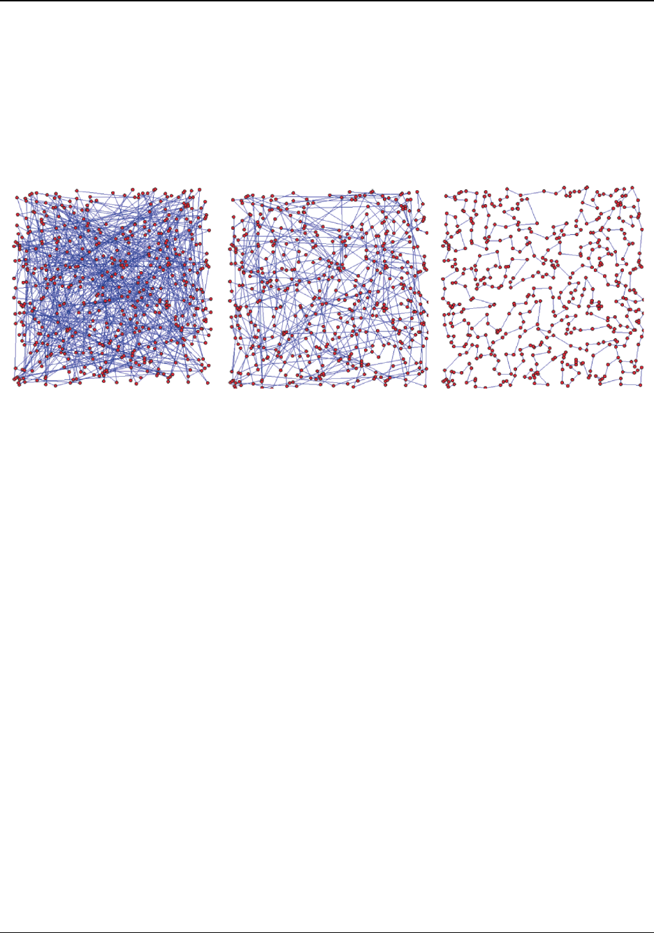
fixed in time and do not evolve. Consider the famous “traveling salesmen” problem shown in Fig.
Revised December 10, 2014 | NOT FOR DISTRIBUTION Page 1
CE 191 — CEE Systems Analysis Professor Scott Moura — University of California, Berkeley
1. The goal is to find the shortest path to loop through N cities, ending at the origin city. Due to
the number of constraints, possible decision variables, and nonlinearity of the problem structure,
the traveling salesmen problem is notoriously difficult to solve.
It turns out that a more efficient solution method exists, specifically designed for multi-stage
decision processes, known as dynamic programming. The basic premise is to break the problem
into simpler subproblems. This structure is inherent in multi-decision processes.
Figure 1: Random (left), suboptimal (middle), and optimal solutions (right).
1.1 Principle of Optimality
Consider a multi-stage decision process, i.e. an equality constrained NLP with dynamics
min
x
k
,u
k
J =
N−1
X
k=0
g
k
(x
k
, u
k
) + g
N
(x
N
) (1)
s. to x
k+1
= f(x
k
, u
k
), k = 0, 1, · · · , N − 1 (2)
x
0
= x
init
(3)
where k is the discrete time index, x
k
is the state at time k, u
k
is the control decision applied at
time k, N is the time horizon, g
k
(·, ·) is the instantaneous cost, and g
N
(·) is the final or terminal
cost.
In words, the principle of optimality is the following. Assume at time step k, you know all the
future optimal decisions, i.e. u
∗
(k + 1), u
∗
(k + 2), · · · , u
∗
(N − 1). Then you may compute the best
solution for the current time step, and pair with the future decisions. This can be done recursively
by starting from the end N − 1, and working your way backwards.
Mathematically, the principle of optimality can be expressed precisely as follows. Define V
k
(x
k
)
as the optimal “cost-to-go” (a.k.a. “value function”) from time step k to the end of the time horizon
N, given the current state is x
k
. Then the principle of optimality can be written in recursive form
Revised December 10, 2014 | NOT FOR DISTRIBUTION Page 2
CE 191 — CEE Systems Analysis Professor Scott Moura — University of California, Berkeley
as:
V
k
(x
k
) = min
u
k
{g(x
k
, u
k
) + V
k+1
(x
k+1
)} , k = 0, 1, · · · , N − 1 (4)
with the boundary condition
V
N
(x
N
) = g
N
(x
N
) (5)
The admittedly awkward aspects are:
1. You solve the problem backward!
2. You solve the problem recursively!
Let us illustrate this with two examples.
A
B
C
D
E
F
G
H
2
4
4
6
5
1
5
11
4
7
1
3
2
2
5
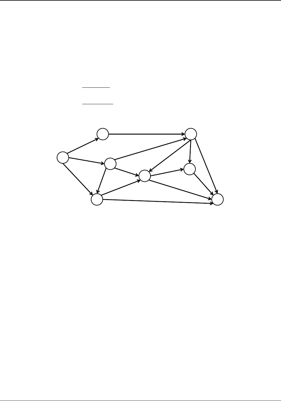
Figure 2: Network for shortest path problem in Example 1.1.
Example 1.1 (Shortest Path Problem). Consider the network shown in Fig. 2. The goal is to find
the shortest path from node A to node H, where path length is indicated by the edge numbers.
Let us define the cost-to-go as V (i). That is, V (i) is the shortest path length from node i to
node H. For example V (H) = 0. Let c(i, j) denote the cost of traveling from node i to node j.
For example, c(C, E) = 7. Then c(i, j) + V (j) represents the cost of traveling from node i to node
j, and then from node j to H along the shortest path. This enables us to write the principle of
optimality equation and boundary conditions:
V (i) = min
j∈N
d
i
{c(i, j) + V (j)} (6)
V (H) = 0 (7)
where the set N
d
i
represents the nodes that descend from node i. For example N
d
C
= {D, E, F }.
We can solve these equations recursively, starting from node H and working our way backward to
node A as follows:
V (G) = c(G, H) + V (H) = 2 + 0 = 2
Revised December 10, 2014 | NOT FOR DISTRIBUTION Page 3

CE 191 — CEE Systems Analysis Professor Scott Moura — University of California, Berkeley
V (E) = min {c(E, G) + V (G), c(E, H) + V (H)} = min {3 + 2, 4 + 0} = 4
V (F ) = min {c(F, G) + V (G), c(F, H) + V (H), c(F, E) + V (E)}
= min {2 + 2, 5 + 0, 1 + 4} = 4
V (D) = min {c(D, E) + V (E), c(D, H) + V (H)} = min {5 + 4, 11 + 0} = 9
V (C) = min {c(C, F ) + V (F ), c(C, E) + V (E), c(C, D) + V (D)}
= min {5 + 4, 7 + 4, 1 + 9} = 9
V (B) = c(B, F ) + V (F ) = 6 + 4 = 10
V (A) = min {c(A, B) + V (B), c(A, C) + V (C), c(A, D) + V (D)}
= min {2 + 10, 4 + 9, 4 + 9} = 12
Consequently, we arrive at the optimal path A → B → F → G → H.
Example 1.2 (Optimal Consumption and Saving). This example is popular among economists for
learning dynamic programming, since it can be solved by hand. Consider a consumer who lives
over periods k = 0, 1, · · · , N and must decide how much of a resource they will consume or save
during each period.
Let c
k
be the consumption in each period and assume consumption yields utility ln(c
k
) over
each period. The natural logarithm function models a “diseconomies of scale” in marginal value
when increasing resource consumption. Let x
k
denote the resource level in period k, and x
0
denote the initial resource level. At any given period, the resource level in the next period is given
by x
k+1
= x
k
− c
k
. We also constrain the resource level to be non-negative. The consumer’s
decision problem can be written as
max
x
k
,c
k
J =
N−1
X
k=0
ln(c
k
) (8)
s. to x
k+1
= x
k
− c
k
, k = 0, 1, · · · , N − 1 (9)
x
k
≥ 0, k = 0, 1, · · · , N (10)
Note that the objective function is not linear nor quadratic in decision variables x
k
, c
k
. It is,
in fact, concave in c
k
. The equivalent minimization problem would be min
x
k
,c
k
− ln(c
k
) which is
convex in c
k
. Moreover, all constraints are linear. Consequently, convex programming is one
solution option. Dynamic programming is another. In general DP does not require the convex
assumptions, and – in this case – can solve the problem analytically.
First we define the value function. Let V
k
(x
k
) denote the maximum total utility from time step k
to terminal time step N, where the resource level in step k is x
k
. Then the principle of optimality
Revised December 10, 2014 | NOT FOR DISTRIBUTION Page 4

CE 191 — CEE Systems Analysis Professor Scott Moura — University of California, Berkeley
equations can be written as:
V
k
(x
k
) = max
c
k
≤x
k
{ln(c
k
) + V
k+1
(x
k+1
)} , k = 0, 1, · · · , N − 1 (11)
with the boundary condition that represents zero utility can be accumulated after the last time step.
V
N
(x
N
) = 0 (12)
We now solve the DP equations starting from the last time step and working backward. Con-
sider k = N − 1,
V
N−1
(x
N−1
) = max
c
N −1
≤x
N −1
{ln(c
N−1
) + V
N
(x
N
)}
= max
c
N −1
≤x
N −1
{ln(c
N−1
) + 0}
= ln(x
N−1
)
In words, the optimal action is to consume all remaining resources, c
∗
N−1
= x
N−1
. Moving on to
k = N − 2,
V
N−2
(x
N−2
) = max
c
N −2
≤x
N −2
{ln(c
N−2
) + V
N−1
(x
N−1
)}
= max
c
N −2
≤x
N −2
{ln(c
N−2
) + V
N−1
(x
N−2
− c
N−2
)}
= max
c
N −2
≤x
N −2
{ln(c
N−2
) + ln(x
N−2
− c
N−2
)}
= max
c
N −2
≤x
N −2
ln (c
N−2
(x
N−2
− c
N−2
))
= max
c
N −2
≤x
N −2
ln
x
N−2
c
N−2
− c
2
N−2
Since ln(·) is a monotonically increasing function, maximizing its argument will maximize its value.
Therefore, we focus on finding the maximum of the quadratic function w.r.t. c
N−2
embedded
inside the argument of ln(·). It’s straight forward to find c
∗
N−2
=
1
2
x
N−2
. Moreover, V
N−2
(x
N−2
) =
ln(
1
4
x
2
N−2
). Continuing with k = N − 3,
V
N−3
(x
N−3
) = max
c
N −3
≤x
N −3
{ln(c
N−3
) + V
N−2
(x
N−2
)}
= max
c
N −3
≤x
N −3
{ln(c
N−3
) + V
N−2
(x
N−3
− c
N−3
)}
= max
c
N −3
≤x
N −3
ln(c
N−3
) + ln
1
4
(x
N−3
− c
N−3
)
2
= max
c
N −3
≤x
N −3
ln(c
N−3
) + ln
(x
N−3
− c
N−3
)
2
− ln(4)
= max
c
N −3
≤x
N −3
ln
x
2
N−3
c
N−3
− 2x
N−3
c
2
N−3
+ c
3
N−3
− ln(4)
Revised December 10, 2014 | NOT FOR DISTRIBUTION Page 5

CE 191 — CEE Systems Analysis Professor Scott Moura — University of California, Berkeley
Again, we can focus on maximizing the argument of ln(·). It’s simple to find that c
∗
N−3
=
1
3
x
N−3
.
Moreover, V
N−3
(x
N−3
) = ln(
1
27
x
3
N−3
). At this point, we recognize the pattern
c
∗
k
=
1
N − k
x
k
, k = 0, · · · , N − 1 (13)
One can use induction to prove this hypothesis indeed solves the recursive principle of optimality
equations. Equation (13) provides the optimal state feedback policy. That is, the optimal policy is
written as a function of the current resource level x
k
. If we write the optimal policy in open-loop
form, it turns out the optimal consumption is the same at each time step. Namely, it is easy to
show that (13) emits the policy
c
∗
k
=
1
N
x
0
, ∀ k = 0, · · · , N − 1 (14)
As a consequence, the optimal action is to consume that same amount of resource at each time-
step. It turns out one should consume 1/N · x
0
at each time step if they are to maximize total
utility.
Remark 1.1. This is a classic example in resource economics. In fact, this example represents
the non-discounted, no interest rate version of Hotelling’s Law, a theorem in resource economics
[1]. Without a discount/interest rate, any difference in marginal benefit could be arbitraged to
increase net benefit by waiting until the next time-step. Embellishments of this problem get more
interesting where there exists uncertainty about resource availability, extraction cost, future benefit,
and interest rate. In fact, oil companies use this exact analysis to determine when to drill an oil
field, and how much to extract.
2 Example 1: Knapsack Problem
The “knapsack” problem is a famous problem which illustrates sequential decision making. Con-
sider a knapsack that has finite volume of K units. We can fill the knapsack with an integer number
of items, x
i
, where there are N types of items. Each item has per unit volume v
i
, and per unit value
of c
i
. Our goal is to determine the number of items x
i
to place in the knapsack to maximize total
value.
This problem is a perfect candidate for DP. Namely, if we consider sequentially filling the knap-
sack one item at a time, then it is easy to understand that deciding which item to include now
impacts what items we can include later. To formulate the DP problem, we define a “state” for the
system. In particular, define y as the remaining volume in the knapsack. At the beginning of the
filling process, the remaining volume is y = K. Consider how the state y evolves when items are
added. Namely, the state evolves according to y − v
i
if we include one unit of item i. Clearly, we
cannot include units whose volume exceeds the remaining volume, i.e. v
i
≤ y. Moreover, the value
Revised December 10, 2014 | NOT FOR DISTRIBUTION Page 6
CE 191 — CEE Systems Analysis Professor Scott Moura — University of California, Berkeley
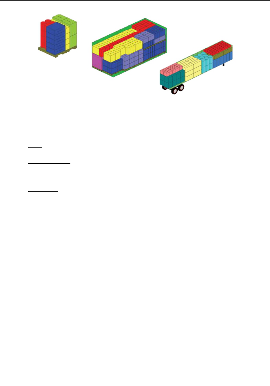
Figure 3: A logistics example of the knapsack problem is optimally packing freight containers.
of the knapsack increases by c
i
for including one unit of item i. We summarize mathematically,
• The state y represents the remaining free volume in the knapsack
• The state dynamics are y − v
i
• The value accrued (i.e. negative cost-per-stage) is c
i
• The initial state is K
• The items we may add are constrained by volume, i.e. v
i
≤ y.
We now carefully define the value function. Let V (y) represent the maximal possible knapsack
value for the remaining volume, given that the remaining volume is y. For example, when the
remaining volume is zero, then the maximum possible value of that remaining volume is zero. We
can now write the principle of optimality and boundary condition:
V (y) = max
v
i
≤y, i∈{1,··· ,N }
{c
i
+ V (y − v
i
)} , (15)
V (0) = 0. (16)
Into the Wilderness Example
To make the knapsack problem more concrete, we consider the “Into the Wilderness” example.
Chris McCandless is planning a trip into the wilderness
1
. He can take along one knapsack and
must decide how much food and equipment to bring along. The knapsack has a finite volume.
However, he wishes to maximize the total “value” of goods in the knapsack.
max 2x
1
+ x
2
[Maximize knapsack value] (17)
1
Inspired by the 1996 non-fictional book “Into the Wild” written by Jon Krakauer. It’s a great book!
Revised December 10, 2014 | NOT FOR DISTRIBUTION Page 7

CE 191 — CEE Systems Analysis Professor Scott Moura — University of California, Berkeley
s. to x
0
+ 2x
1
+ 3x
2
= 9 [Finite knapsack volume] (18)
x
i
≥ 0 ∈ Z [Integer number of units] (19)
Note that we have the following parameters: x
i
is the integer number of goods; i = 1 represents
food, i = 2 represents equipment, and suppose i = 0 represents empty space; the knapsack
volume is K = 9; the per unit item values are c
0
= 0, c
1
= 2, c
2
= 1; the per unit item volumes are
v
0
= 1, v
1
= 2, v
2
= 3.
Now we solve the DP problem recursively, using (15) and initializing the recursion with bound-
ary condition (16).
V (0) = 0
V (1) = max
v
i
≤1
{c
i
+ V (1 − v
i
)} = max {0 + V (1 − 1)} = 0
V (2) = max
v
i
≤2
{c
i
+ V (2 − v
i
)}
= max {0 + V (2 − 1), 2 + V (2 − 2)} = 2
V (3) = max
v
i
≤3
{c
i
+ V (3 − v
i
)}
= max {0 + V (3 − 1), 2 + V (3 − 2), 1 + V (3 − 3)} = 2
V (4) = max
v
i
≤4
{c
i
+ V (4 − v
i
)}
= max {0 + V (4 − 1), 2 + V (4 − 2), 1 + V (4 − 3)} = max{2, 2 + 2, 1 + 0} = 4
V (5) = max
v
i
≤5
{c
i
+ V (5 − v
i
)}
= max {0 + V (5 − 1), 2 + V (5 − 2), 1 + V (5 − 3)} = max{4, 2 + 2, 1 + 2} = 4
V (6) = max
v
i
≤6
{c
i
+ V (6 − v
i
)}
= max {0 + V (6 − 1), 2 + V (6 − 2), 1 + V (6 − 3)} = max{4, 2 + 4, 1 + 2} = 6
V (7) = max
v
i
≤7
{c
i
+ V (7 − v
i
)}
= max {0 + V (7 − 1), 2 + V (7 − 2), 1 + V (7 − 3)} = max{6, 2 + 4, 1 + 4} = 6
V (8) = max
v
i
≤8
{c
i
+ V (8 − v
i
)}
= max {0 + V (8 − 1), 2 + V (8 − 2), 1 + V (8 − 3)} = max{6, 2 + 6, 1 + 4} = 8
V (9) = max
v
i
≤9
{c
i
+ V (9 − v
i
)}
= max {0 + V (9 − 1), 2 + V (9 − 2), 1 + V (9 − 3)} = max{8, 2 + 6, 1 + 6} = 8
V (9) = 8
Consequently, we find the optimal solution is to include 4 units of food, 0 units of equipment, and
there will be one unit of space remaining.
Revised December 10, 2014 | NOT FOR DISTRIBUTION Page 8

CE 191 — CEE Systems Analysis Professor Scott Moura — University of California, Berkeley
3 Example 2: Smart Appliance Scheduling
In this section, we utilize dynamic programming principles to schedule a smart dishwasher ap-
pliance. This is motivated by the vision of future homes with smart appliances. Namely, internet-
connected appliances with local computation will be able to automate their procedures to minimize
energy consumption, while satisfying homeowner needs.
Consider a smart dishwasher that has five cycles, indicated in Table 1. Assume each cycle
requires 15 minutes. Moreover, each cycle must be run in order, possibly with idle periods in
between. We also consider electricity price which varies in 15 minute periods, as shown in Fig.
4. The goal is to find the cheapest cycle schedule starting at 17:00 and ending at 24:00, with the
requirement that the dishwasher completes all of its cycles by 24:00 midnight.
3.1 Problem Formulation
Let us index each 15 minute time period by k, where k = 0 corresponds to 17:00 – 17:15, and k =
N = 28 corresponds to 24:00–00:15. Let us denote the dishwasher state by x
k
∈ {0, 1, 2, 3, 4, 5},
which indicates the last completed cycle at the very beginning of each time period. The initial state
is x
0
= 0. The control variable u
k
∈ {0, 1} corresponds to either wait, u
k
= 0, or continue to the
next cycle, u
k
= 1. We assume control decisions are made at the beginning of each period, and
cost is accrued during that period. Then the state transition function, i.e. the dynamical relation, is
given by
x
k+1
= x
k
+ u
k
, k = 0, · · · , N − 1 (20)
Let c
k
represent the time varying cost in units of USD/kWh. Let p(x
k
) represent the power required
for cycle x
k
, in units of kW. We are now positioned to write the optimization program
min
N−1
X
k=0
1
4
c
k
p(x
k
+ u
k
) u
k
s. to x
k+1
= x
k
+ u
k
, k = 0, · · · , N − 1
x
0
= 0,
x
N
= 5,
u
k
∈ {0, 1}, k = 0, · · · , N − 1
3.2 Principle of Optimality
Next we formulate the dynamic programming equations. The cost-per-time-step is given by
g
k
(x
k
, u
k
) =
1
4
c
k
p(x
k
+ u
k
) u
k
, (21)
Revised December 10, 2014 | NOT FOR DISTRIBUTION Page 9

CE 191 — CEE Systems Analysis Professor Scott Moura — University of California, Berkeley
=
1
4
c
k
p(x
k
+ u
k
) u
k
, k = 0, · · · , N − 1 (22)
Since we require the dishwasher to complete all cycles by 24:00, we define the following terminal
cost:
g
N
(x
N
) =
(
0 : x
N
= 5
∞ : otherwise
(23)
Let V
k
(x
k
) represent the minimum cost-to-go from time step k to final time period N, given the last
completed dishwasher cycle is x
k
. Then the principle of optimality equations are:
V
k
(x
k
) = min
u
k
∈{0,1}
1
4
c
k
p(x
k
+ u
k
)u
k
+ V
k+1
(x
k+1
)
= min
u
k
∈{0,1}
1
4
c
k
p(x
k
+ u
k
)u
k
+ V
k+1
(x
k
+ u
k
)
= min
V
k+1
(x
k
),
1
4
c
k
p(x
k
+ 1) + V
k+1
(x
k
+ 1)
(24)
with the boundary condition
V
N
(5) = 0, V
N
(i) = ∞ for i 6= 5 (25)
We can also write the optimal control action as:
u
∗
(x
k
) = arg min
u
k
∈{0,1}
1
4
c
k
p(x
k
+ u
k
)u
k
+ V
k+1
(x
k
+ u
k
)
Equation (24) is solved recursively, using the boundary condition (25) as the first step. Next, we
show how to solve this algorithmically in Matlab.
3.3 Matlab Implementation
The code below provides an implementation of the dynamic programming equations.
1 %% Problem Data
2 % Cycle power
3 p = [0; 1.5; 2.0; 0.5; 0.5; 1.0];
4
5 % Electricity Price Data
6 c = [12,12,12,10,9,8,8,8,7,7,6,5,5,5,5,5,5,5,6,7,7,8,9,9,10,11,11,...
7 12,12,14,15,15,16,17,19,19,20,21,21,22,22,22,20,20,19,17,15,15,16,...
8 17,17,18,18,16,16,17,17,18,20,20,21,21,21,20,20,19,19,18,17,17,...
9 16,19,21,22,23,24,26,26,27,28,28,30,30,30,29,28,28,26,23,21,20,18,18,17,17,16,16];
10
Revised December 10, 2014 | NOT FOR DISTRIBUTION Page 10
CE 191 — CEE Systems Analysis Professor Scott Moura — University of California, Berkeley
cycle power
1 prewash 1.5 kW
2 main wash 2.0 kW
3 rinse 1 0.5 kW
4 rinse 2 0.5 kW
5 dry 1.0 kW
00:00 04:00 08:00 12:00 16:00 20:00 24:00
0
5
10
15
20
25
30
35
Time of Day
Electricity Cost [cents/kWh]
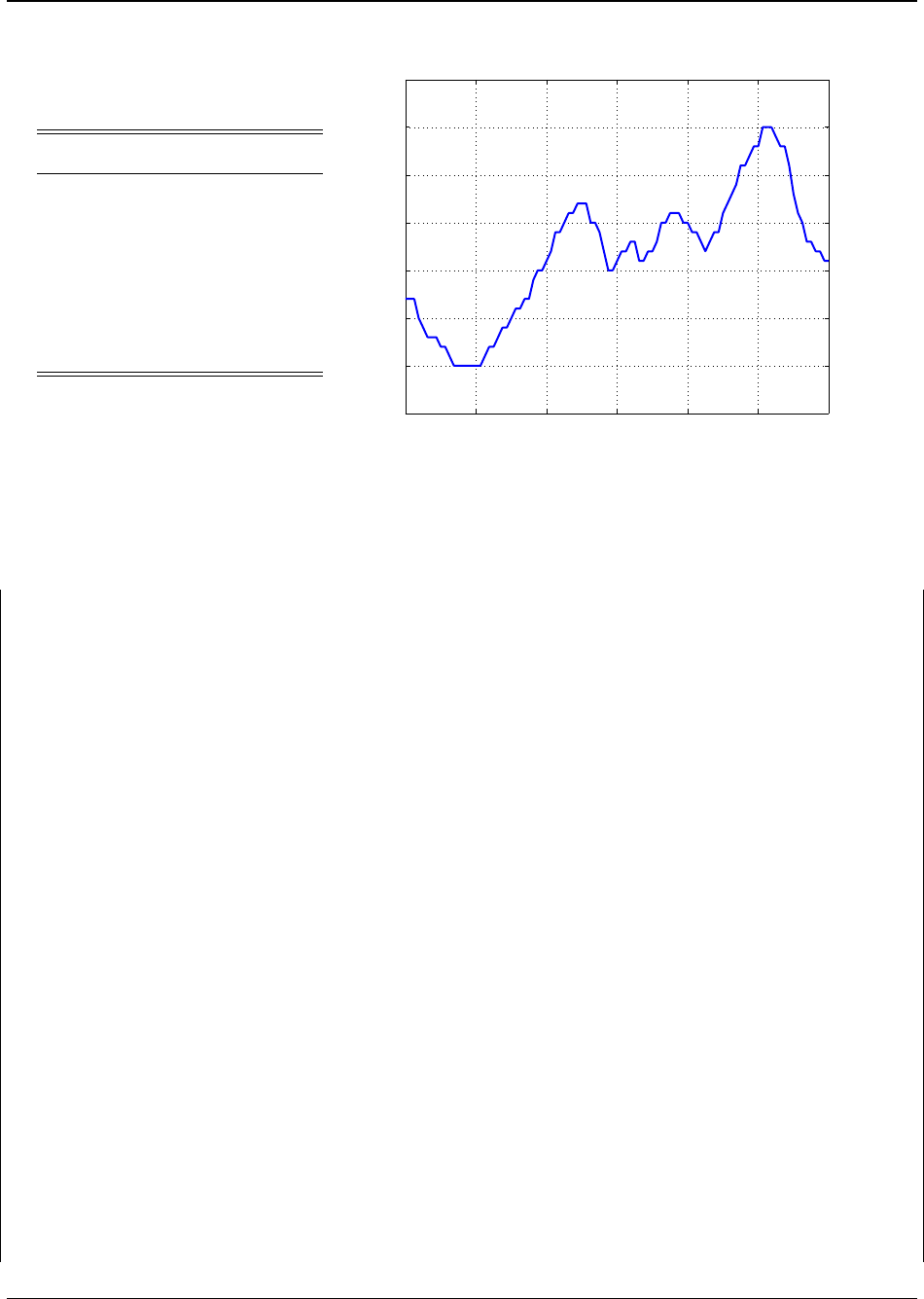
Figure 4 & Table 1: [LEFT] Dishwasher cycles and corresponding power consumption. [RIGHT] Time-
varying electricity price. The goal is to determine the dishwasher schedule between 17:00 and 24:00 that
minimizes the total cost of electricity consumed.
11 %% Solve DP Equations
12 % Time Horizon
13 N = 28;
14 % Number of states
15 nx = 6;
16
17 % Preallocate Value Function
18 V = inf
*
ones(N,nx);
19 % Preallocate control policy
20 u = nan
*
ones(N,nx);
21
22 % Boundary Condition
23 V(end, end) = 0;
24
25 % Iterate through time backwards
26 for k = (N−1):−1:1;
27
28 % Iterate through states
29 for i = 1:nx
30
31 % If you're in last state, can only wait
32 if(i == nx)
33 V(k,i) = V(k+1,i);
34
35 % Otherwise, solve Principle of Optimality
36 else
Revised December 10, 2014 | NOT FOR DISTRIBUTION Page 11
CE 191 — CEE Systems Analysis Professor Scott Moura — University of California, Berkeley
00:00 04:00 08:00 12:00 16:00 20:00 24:00
0
5
10
15
20
25
30
35
Time of Day
Electricity Cost [cents/kWh]
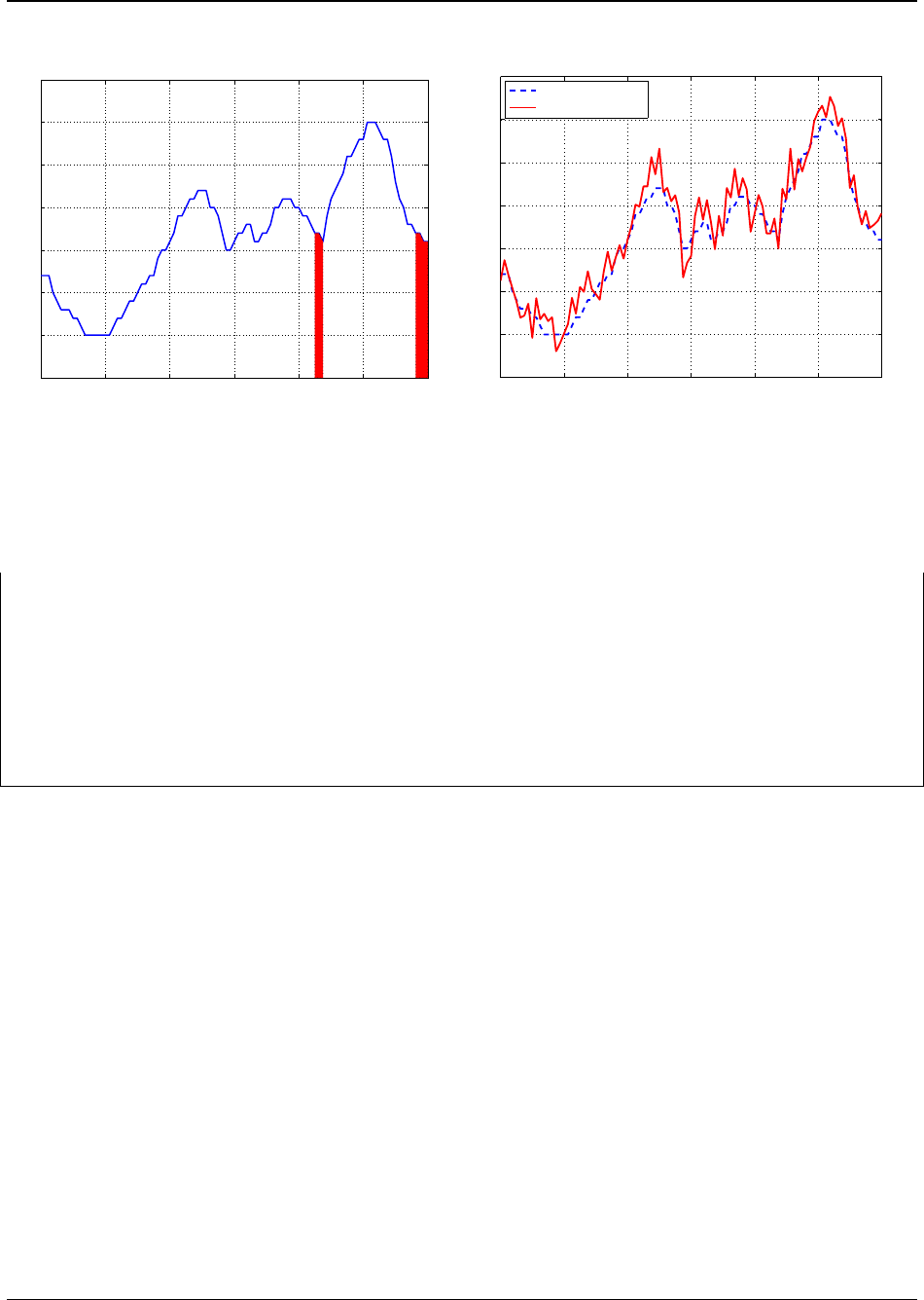
Figure 5: The optimal dishwasher schedule is to
run cycles at 17:30, 17:45, 23:15, 23:30, 23:45.
The minimum total cost of electricity is 22.625
cents.
00:00 04:00 08:00 12:00 16:00 20:00 24:00
0
5
10
15
20
25
30
35
Time of Day
Electricity Cost [cents/kWh]
Forecasted Price
Real Price
Figure 6: The true electricity price c
k
can be ab-
stracted as a forecasted price plus random uncer-
tainty.
37 %Choose u=0 ; u=1
38 [V(k,i),idx] = min([V(k+1,i); 0.25
*
c(69+k)
*
p(i+1) + V(k+1,i+1)]);
39
40 % Save minimizing control action
41 u(k,i) = idx−1;
42 end
43 end
44 end
Note the value function is solved backward in time (line 26), and for each state (line 29). The
principle of optimality equation is implemented in line 38, and the optimal control action is saved
in line 41. The variable u(k,i) ultimately provides the optimal control action as a function of time
step k and dishwasher state i, namely u
∗
k
= u
∗
(k, x
k
).
3.4 Results
The optimal dishwasher schedule is depicted in Fig. 5, which exposes how cycles are run in
periods of low electricity cost c
k
. Specifically, the dishwasher begins prewash at 17:30, main wash
at 17:45, rinse 1 at 23:15, rinse 2 at 23:30, and dry at 23:45. The total cost of electricity consumed
is 22.625 cents.
Revised December 10, 2014 | NOT FOR DISTRIBUTION Page 12

CE 191 — CEE Systems Analysis Professor Scott Moura — University of California, Berkeley
4 Stochastic Dynamic Programming
The example above assumed the electricity price c
k
for k = 0, · · · , N is known exactly a priori.
In reality, the smart appliance may not know this price signal exactly, as demonstrated by Fig. 6.
However, we may be able to anticipate it by forecasting the price signal, based upon previous data.
We now seek to relax the assumption of perfect a priori knowledge of c
k
. Instead, we assume that
c
k
is forecasted using some method (e.g. machine learning, neural networks, Markov chains) with
some error with known statistics..
We shall now assume the true electricity cost is given by
c
k
= ˆc
k
+ w
k
, k = 0, · · · , N − 1 (26)
where ˆc
k
is the forecasted price that we anticipate, and w
k
is a random variable representing
uncertainty between the forecasted value and true value. We additionally assume knowledge of
the mean uncertainty, namely E[w
k
] = w
k
for all k = 0, · · · , N. That is, we have some knowledge
of the forecast quality, quantified in terms of mean error.
Armed with a forecasted cost and mean error, we can formulate a stochastic dynamic program-
ming (SDP) problem:
min J = E
w
k
"
N−1
X
k=0
1
4
(ˆc
k
+ w
k
) p(x
k+1
) u
k
#
s. to x
k+1
= x
k
+ u
k
, k = 0, · · · , N − 1
x
0
= 0,
x
N
= 5,
u
k
∈ {0, 1}, k = 0, · · · , N − 1
where the critical difference is the inclusion of w
k
, a stochastic term. As a result, we seek to
minimize the expected cost, w.r.t. to random variable w
k
.
We now formulate the principle of optimality. Let V
k
(x
k
) represent the expected minimum cost-
to-go from time step k to N, given the current state x
k
. Then the principle of optimality equations
can be written as:
V
k
(x
k
) = min
u
k
E {g
k
(x
k
, u
k
, w
k
) + V
k+1
(x
k+1
)}
= min
u
k
∈{0,1}
E
1
4
(ˆc
k
+ w
k
) p(x
k+1
)u
k
+ V
k+1
(x
k+1
)
= min
u
k
∈{0,1}
1
4
(ˆc
k
+ w
k
) p(x
k+1
)u
k
+ V
k+1
(x
k
+ u
k
)
= min
V
k+1
(x
k
),
1
4
(ˆc
k
+ w
k
) p(x
k
+ 1) + V
k+1
(x
k
+ 1)
Revised December 10, 2014 | NOT FOR DISTRIBUTION Page 13

CE 191 — CEE Systems Analysis Professor Scott Moura — University of California, Berkeley
with the boundary condition
V
N
(5) = 0, V
N
(i) = ∞ for i 6= 5
These equations are deterministic, and can be solved exactly as before. The crucial detail is that
we have incorporated uncertainty by incorporating a forecasted cost with uncertain error. As a
result, we seek to minimize expected
cost.
5 Notes
An excellent introductory textbook for learning dynamic programming is written by Denardo [2]. A
more complete reference for DP practitioners is the two-volume set by Bertsekas [3]. DP is used
across a broad set of applications, including maps, robot navigation, urban traffic planning, net-
work routing protocols, optimal trace routing in printed circuit boards, human resource scheduling
and project management, routing of telecommunications messages, hybrid electric vehicle energy
management, and optimal truck routing through given traffic congestion patterns. The applications
are quite literally endless. As such, the critical skill is identifying a DP problem and abstracting an
appropriate formalization.
References
[1] H. Hotelling, “Stability in competition,” The Economic Journal, vol. 39, no. 153, pp. pp. 41–57, 1929.
[2] E. V. Denardo, Dynamic programming: models and applications. Courier Dover Publications, 2003.
[3] D. P. Bertsekas, D. P. Bertsekas, D. P. Bertsekas, and D. P. Bertsekas, Dynamic programming and
optimal control. Athena Scientific Belmont, MA, 1995, vol. 1, no. 2.
Revised December 10, 2014 | NOT FOR DISTRIBUTION Page 14
