
Working Paper Series
The impact of the ECB’s targeted
long-term refinancing operations
on banks’ lending policies:
the role of competition
Desislava C. Andreeva, Miguel García-Posada
Disclaimer: This paper should not be reported as representing the views of the European Central Bank
(ECB). The views expressed are those of the authors and do not necessarily reflect those of the ECB.
No 2364 / January 2020
Abstract
We assess the impact of the Eurosystem’s Targeted Long-Term
Refinancing Operations (TLTROs) on
the lending policies of euro area banks. We first build a theoretical model in which banks compete in
the credit and deposit markets. We distinguish between direct and indirect effects. Direct effects
take place because bidding banks expand their loan supply due to the lower marginal costs implied
by the TLTROs. Indirect effects on non-bidders operate via changes in the competitive environment
in banks’ credit and deposit markets. We then test these predictions with a sample of 130 banks
from 13 countries focusing on the first TLTRO series. Regarding direct effects, we find an easing
impact on margins on loans to relatively safe borrowers, but no impact on credit standards.
Regarding indirect effects, there is a positive impact on the loan supply on non-bidders which
operates via an easing of credit standards.
JEL Classification: G21, E52, E58
Keywords: unconventional monetary policy; TLT
ROs; lending policies; competition
ECB Working Paper Series No 2364 / January 2020
1
Non-technical summary
The TLTROs are one of the non-standard monetary policy measures introduced by the ECB in the
course of the financial crisis to stimulate the supply of bank loans to the real economy. In these
operations banks could borrow money from the Eurosystem for up to four years at very attractive
interest rates. The maximum amount that could be borrowed was linked to a specific category of
bank loans (‘targeted’ or ‘eligible’ loans). These are bank loans to euro area households and non-
financial firms except for household mortgages. This link intends to ensure that the stimulus reaches
the real economy. This paper evaluates the impact of the TLTROs on the lending policies of euro area
banks, focusing on the first TLTRO series announced in June 2014.
Our analysis aims to capture both the direct impact of the measure on the lending policies of banks
which accessed the TLTROs and the indirect effects, as the remaining banks react to the change in
the behaviour of TLTRO bidders. Such indirect effects operate via changes in the competitive
environment in banks’ credit and funding markets. Their inclusion as object for analysis is a distinct
feature of this study.
The paper first presents a simple extension of the standard Monti-Klein model of bank competition.
For the sake of simplicity, the model features two banks. One of them is perceived to be risky and
thus faces higher funding costs. In the model only the risky bank bids in the TLTROs since thereby it
can lower its overall funding costs. The asymmetric recourse to the TLTROs allows us to study the
direct impact of the measure on the risky bank, which borrows from the central bank, and the
indirect impact on its competitor, the safe bank.
The model predicts a positive impact of the TLTROs on the bidding bank. The decline in its funding
costs allows it to expand its supply of loans. By contrast, the impact on the other bank is ex ante
ambiguous. On the one hand the risky bank is able to attract customers which in the absence of the
TLTROs the safe bank would have served, suggesting a negative impact. On the other hand, it also
indirectly lowers the funding costs of the safe bank, supporting its supply of bank loans. This indirect
effect arises as the risky bank demands less market funding, resulting in lower market funding costs
for the entire banking system, including the safe bank.
Our empirical analysis finds that the TLTROs had a positive impact on bank loan supply both directly
– on the bidders – and indirectly on their competitors. We find strong indirect effects of the TLTROs
on credit standards, but no significant impact on margins on safe loans. In the case of loans to
ECB Working Paper Series No 2364 / January 2020
2
enterprises, the impact is stro
nger for large firms. We also find some evidence that the TLTROs do
not lead to excessive risk taking, as TLTRO uptakes are negatively correlated with the probability of
narrowing margins on riskier loans. Regarding direct effects, the meas
ure affected mainly the
margins on loans to relatively safe borrowers. Moreover, the finding is mainly driven by adjustments
in the lending policy by banks which bid for larger amounts compared to those which borrowed less
from the TLTROs (i.e., the intensive margin of monetary policy pass-through) as opposed to
differences between bidders and non-bidd
ers (i.e., the extensive margin).
ECB Working Paper Series No 2364 / January 2020
3

1. Introduction
Since the 2008 global financial crisis, central banks around the world have undertaken nume
rous
unconventional monetary policies to prevent a credit crunch, stimulate aggregate demand and boost
inflation. In the euro area these included the provision of liquidity using fixed-rate full-allotment
tenders, a lengthening of the maturity of central bank credit operations, a wider set of eligible
collateral, large scale purchase programmes of public and private sector assets, negative interest
rates and forward guidance.
The goal of this paper is to assess the impact
of the Eurosystem’s Targeted Long-Term Refinancing
Operations (TLTROs) on the lending policies of euro area banks. The TLTROs are liquidity providing
central bank operations with maturity of up to four years. They were announced in June 2014 in a
context of slow economic growth, weak inflation outlook and subdued monetary and credit dynamics
in the euro area. Unlike their predecessors (VLTROs
4
), the TLTROs explicitly targeted lending to the
real economy and were designed to reduce the incentives to banks to use the liquidity for sovereign
debt purchases. Our analysis aims to capture both the direct impact of the measure on the lending
policies of banks which accessed the TLTROs and the indirect effects, as the remaining banks react
strategically to the change in the behaviour of TLTRO bidders. Such indirect effects operate via
changes in the competitive environment in banks’ credit and funding markets. Their inclusion as
object for analysis is a distinct feature of this study.
To guide our empirical research, we first present a simple extensi
on of the Monti-Klein model of
oligopolistic competition in the banking sector. For the sake of simplicity, we consider only two
banks, a safe and a risky bank, which compete à la Cournot in the loan and deposit markets. The
main departure from the standard model is the introduction of a funding impairment: one of the
banks is perceived to be risky, resulting in higher funding costs. Importantly, it also leads to an
asymmetric recourse to the TLTROs and allows us to study the direct impact of the measure on the
risky bank, which borrows from the central bank, and the indirect impact on its competitor, the safe
bank.
This asymmetric recourse arises as the TLT
ROs borrowing costs are assumed to be higher than the
deposit funding costs of the safe bank but attractive for its risky competitor. After the introduction of
4
Longer-term refinancing operations with a three year maturity implemented in December 2011 and February
2012. The abbreviations “VLTROs” stands for very long-term refinancing operations.
ECB Working Paper Series No 2364 / January 2020
4
the measure the
risky bank can fund part of its loan portfolio with the TLTROs rather than with more
costly deposits. The introduction of the TLTROs has both direct effects on the bidding bank (the risky
bank) and indirect effects on the non-bidder (the safe bank). Regarding direct effects, the funding
cost relief due to the TLTROs leads to an expansion of the loan supply by the risky bank. With respect
to indirect effects, we must differentiate between two opposite forces. On the one hand,
competition in the credit market becomes stronger. The TLTROs, by reducing the risky bank’s
marginal funding costs, allows it to compete more aggressively in the loan market. As banks compete
à la Cournot, loan quantities are strategic substitutes, implying that an expansion in the credit supply
of the risky bank leads to a contraction in the credit supply of the safe bank. On the other hand,
competition in the deposit market weakens because the risky bank substitutes some deposits with
TLTRO funding. The lower demand for deposits leads to lower deposit rates, which translate into
lower marginal costs also for the safe bank. Ceteris paribus, its loan supply expands. Hence, the
overall indirect impact of the TLTROs is a priori ambiguous and must be assessed empirically.
The empirical analysis meas
ures bank lending policies with credit standards (i.e., the internal
guidelines or loan approval criteria of a bank) and loan margins (i.e., the agreed spread over the
relevant reference rate), as reported by banks in the ECB’s Bank Lending Survey (BLS). Several papers
in the literature, such as Lown and Morgan (2006), and Ciccarelli et al. (2015), identify credit
standards as reported in lending surveys as proxies for credit supply. We use the confidential
answers by 130 banks from 13 euro area countries, matched with individual bank balance-sheet
information and proprietary data on banks’ participation in central bank credit operations. Our
empirical analysis of the causal impact of the TLTROs on bank lending policies focuses on the first
series of TLTROs introduced in June 2014, therefore when referring to TLTROs in general we have
TLTRO-I in mind. The identification strategy needs to address two major issues. First, banks
part
icipated in the TLTROs on a voluntary basis and thus selection into treatment is non-ra
ndom. To
obtain consistent estimates we construct an instrumental variable for the TLTRO uptake. The
proposed instrumental variable comes from the institutional setting of TLTRO-I, as in Benetton and
Fantino (2017). In particular, we exploit an allocation rule by the policy, according to which banks
could borrow an amount equivalent to 7% of their eligible loans outstanding on 30 April 2014.
Crucially, the stock of eligible loans was measured at a date prior to the announcement of the policy
(June 2014). The initial allowance constitutes an exogenous component of the TLTRO uptakes, as it is
based on exogenous parameters that are common across banks and on pre-determined bank balance
ECB Working Paper Series No 2364 / January 2020
5

sheet characteristics. The relevance of our instrument is ensured by the fact that in the first two
TLTRO
s-I 80% of the participating banks in our sample borrowed at least 90% of their initial
allowance (Figure 1).
Second, credit supply must be disentangled from credit demand.
5
For instance, banks with high
TLTRO uptakes may face more dynamic demand conditions or deal with more creditworthy
borrowers, which may induce them to ease credit standards or narrow margins. To control for
demand factors, we include a large vector of control variables that measure the evolution of credit
demand by firms and households in the different segments of the credit market (e.g. loans to SMEs),
as well as the factors underlying those developments (e.g., consumer confidence), as reported by
banks in the BLS.
Our results suggest strong indirect effects of the TLTRO-
I on credit standards, but no significant
impact on margins on safe loans. In the case of loans to non-financial c
orporations, a standard
deviation increase in the TLTRO uptakes of a bank’s competitors leads to a 5.3 pp increase in the
probability that it eases overall credit standards. The impact on credit to large firms is even stronger,
resulting in an 8.8 pp increase in the probability of easing credit standards. In the case of loans to
households for house purchase, a standard deviation increase in the TLTRO uptakes of a bank’s
competitors implies an 8.8 pp increase in the probability that the bank eases its own credit
standards. These effects are concentrated in banks with low market share that face high competitive
pressures, suggesting that competition in the credit market plays a crucial role. By contrast, the
TLTRO uptakes of a bank’s competitors have no significant effect on margins on average loans in
either segment. We also find some evidence that the TLTROs did not lead to excessive risk taking, as
TLTRO uptakes are negatively correlated with the probability of narrowing margins on riskier loans.
All in all, the results suggest that the TLTROs generate positive funding externalities on non-bidders.
Regarding direct effects, the t
ransmission of monetary policy takes place mainly through the
adjustment of margins on loans to relatively safe borrowers. The effects are stronger in the
subsample of bidding banks (i.e., the intensive margin of monetary policy pass-through) than in the
5
While the BLS aims to distinguish between supply (measured by credit standards and loan margins) and
demand, note that some of the factors underlying the changes in credit standards and loan margins have a
demand component. According to the survey, credit standards and loan margins are determined by cost of
funds and balance sheet constraints, pressure from competition, bank’s risk tolerance and perception of risk.
The last factor comprises the sub-factors “general economic situation”, “industry or firm-specific situation” and
“risk related to the collateral demanded”.
ECB Working Paper Series No 2364 / January 2020
6

comparison between bidders and non-bid
ders (i.e., the extensive margin). In particular, for the
subsample of bidding banks, a standard deviation increase in a bank’s TLTRO uptake increases the
probability of narrowing margins on average loans to firms by 20 pp and raises the probability of
narrowing margins on average loans to households for house purchase by around 29pp. With respect
to the extensive margin, bidding banks are much more likely (62 pp) to narrow margins on average
loans than non-bidders in the case of housing loans, while there are no significant differences
between the two groups in the segment of corporate loans.
The rest of the paper is organised as follows. Section 2 reviews the most r
elevant literature on the
subject and discusses our key contributions. Section 3 describes the institutional background of the
TLTROs. Section 4 presents a simple theoretical model to guide our empirical analysis. Section 5
discusses the identification strategy in detail. Section 6 explains the data sources and the variables
employed in the empirical analyses. Section 7 comments on the main results. Section 8 explains
some robustness tests. Section 9 concludes.
2. Related Literature and contribution
Our
paper belo
ngs to the broad and by now mature literature on the effects of monetary policy on
bank credit supply, the so-called bank lending channel. It belongs to the set of empirical studies
focusing on the impact on unconventional monetary policies. The analysis is most closely related to
the branch of the literature analysing the impact of large scale liquidity injections via central bank
credit operations, as introduced for instance by the ECB and the Fed in the course of the financial
crisis.
6
Many of the papers using euro area data focus on the two longer-term refinancing operations
with a 3 year maturity (often labelled ‘VLTROs’ or ‘3yLTROs’) of 2011-2012, in which an
unprecedented overall amount of around one trillion euros were allotted to banks in the euro area.
6
Examples of injections of liquidity via central bank credit operations by the Eurosystem include the liquidity-
providing longer-term refinancing operations with a one year maturity announced in May 2009, the longer-
term refinancing operations with a 3 year maturity announced in December 2011 and the two series of TLTROs,
announced in June 2014 and in March 2016. The liquidity providing credit operations introduced by the Fed
include the Primary Dealer Credit Facility, the Term Auction Facility, Asset-Backed Commercial Paper Money
Market Mutual Fund Liquidity Facility, the Commercial Paper Funding Facility, and the Term Asset-Backed
Securities Loan Facility.
ECB Working Paper Series No 2364 / January 2020
7

As regards analyses usin
g aggregate data, Darracq-Paries and De Santis (2015) use information on
credit supply conditions from the ECB's Bank Lending Survey (BLS) to identify the credit supply shock
implied by the VLTROs in a panel-VAR for euro area countries. Their counterfactual experiments
point to a relevant increase in bank loans to non-financial corporations and a moderate narrowing of
lending rate spreads, together with a significant increase in the euro area real GDP. Casiraghi et al.
(2016) use bank-level data and the individual answers of the Italian banks to the BLS, together with
the Bank of Italy model of the Italian economy, to assess the effectiveness of the ECB's Securities
Markets Programme (SMP), the VLTROs and the Outright Monetary Operations (OMT). They find that
the VLTROs had a significant impact on credit supply, mainly through a sizeable reduction in the
interest rates paid by Italian banks in the interbank market. They also find that the overall impact of
the three policies on GDP growth, mainly via the credit channel, was a cumulative increase of 2.7 pp.
over the period 2012–2013.
A different appr
oach consists of exploiting very granular data coming from credit registers to identify
shifts in credit supply using the Khawja and Mian (2008) methodology. Andrade et al. (2015), in their
study of the French banking system, find that the VLTROs had a positive and sizeable impact on the
provision of credit to firms. The opportunity to replace outstanding short-term by longer-term
central bank funding (as banks rolled over their existing borrowings from the Eurosystem into the
VLTROs) enhanced this transmission. Similarly, Jasova et al. (2018), in their analysis of the Portuguese
case, show that the extension of bank debt maturity caused by the VLTROs had a positive and
sizeable impact on bank lending to the real economy thanks to the reduction in rollover risk. Garcia-
Posada and Marchetti (2016) find that the VLTROs had a positive moderate-sized effect on the supply
of bank credit to Spanish firms. The effect was greater for illiquid banks and it was driven by credit to
SMEs, as there was no impact on loans to large firms. Carpinelli and Crosignani (2017), for the case of
Italy, show that banks that experienced a wholesale market dry-up before the intervention reduced
their credit supply during the period of funding stress and restored their credit supply once the
central bank injected liquidity into the system, partly due to a regulatory change that expanded
eligible collateral.
7
While the above evidence suggests that the VLTROs were effective in preventing a credit crunch in
the euro
area, there is also ample evidence that banks used part of the liquidity to purchase high-
7
The Italian government offered banks the possibility to obtain a government guarantee on securities
otherwise ineligible as collateral against a fee.
ECB Working Paper Series No 2364 / January 2020
8
yield government bonds and engage in carry trade strategies (A
charya and Steffen (2015), Carpinelli
and Crosignani (2017), Crosignani et al (2017), Jasova et al. (2018)), which reinforced the sovereign-
bank nexus. Consistent with these findings, Van der Kwaak (2017) builds a DSGE model in which the
provision of central bank liquidity, for which commercial banks pledge collateral in the form of
government bonds, induces banks to shift from private credit to government bonds, and finds that
the cumulative effect on output is zero. Similarly, the model of Corbisiero (2018) shows that the
sovereign-bank nexus can impair a proper monetary transmission mechanism in the euro area,
because in times of high sovereign yields central bank liquidity injections can lead banks in stressed
countries to increase their domestic sovereign holdings, rather than channelling funds to the real
economy.
As a response to those criticisms, the TLTROs explicitly target lending to the real economy.
The
literature on the topic is still scarce. Balfoussia and Gibson (2016) analyse the potential impact of the
TLTROs on the real economic activity of the euro area within a VAR framework. Their results suggest
a significant impact of the TLTROs on economic growth via an easing of financial conditions.
Andreeva (2018) studies the impact of the TLTROs on bank lending rates and volumes in a difference-
in-differences framework. She finds that the TLTROs successfully boosted the supply of eligible bank
loans with limited spill-over effects on not targeted ones. Benetton and Fantino (2017) use the Italian
credit register to analyse the pass-through of the TLTROs to the cost of credit to Italian firms. As in
our paper, they use the initial borrowing allowance as an instrument for the endogenous take-up in
the TLTROs in a diff-in-diff framework. They find that banks participating in the TLTROs decrease
their rates by 20 basis points relative to non-participating banks. Crucially, the pass-through of the
TLTROs depends on the competition in local credit markets, as proxied by the Herfindahl-Hirschman
Index (HHI): a firm in a province with a standard deviation higher level of concentration experiences
almost no decrease in the rates as a result of the liquidity injection.
Our paper, while being
closely related to Benetton and Fantino (2017), possesses four important
distinct features. First, we analyse both the direct and the indirect channel of the transmission of the
TLTROs to the banking sector. Previous literature has focused on the direct channel (the direct
impact of a bank’s participation in the programme on its own credit supply) and has ignored the
indirect channel (the impact of the participation of a bank’s competitors on the bank’s credit supply
via changes in the competitive environment). Second, we analyse the impact of the TLTROs on both
bank credit standards and margins. Confidential survey data allows us to study lending standards, a
ECB Working Paper Series No 2364 / January 2020
9

variable that is not directly observed in credit registers.
8
A related analysis using banks’ individual
responses in the BLS to assess the impact of the APP and negative interest rates can be found in
Altavilla et al (2018a) and Arce et al (2018). Third, we analyse both loans to firms and households,
while previous literature has exclusively studied the former. Finally, we analyse the transmission of
unconventional monetary policy in 13 euro area countries, while the papers that rely on credit
registers only study the effect on a single country.
3. Institutional framework
On the 5th of June 2014, the ECB decided to support bank lending to the euro area nonfinancial
private
sector through a first set of Targeted Longer-Term Refinancing Operations (TLTRO I).
9
This
policy was implemented through eight auctions, one each quarter from September 2014 to June
2016, and participation was open to institutions that were eligible for the Eurosystem open market
operations. In addition, a second and third series of TLTROs (TLTRO-II and III) were announced on the
10
th
of March 2016
10
and 7
th
March 2019 respectively This paper focuses on the effect of TLTRO I on
banks’ lending policies, as measured via credit standards and margins.
All 8 TLTROs-I m
atured in September 2018, although early voluntary repayments could be done
starting 24 months after each TLTRO. The applicable interest rate was fixed over the life of each
operation at the rate on the Eurosystem’s main refinancing operations (MROs) prevailing at the time
of take-up, plus a fixed spread of 10 basis points in the case of the first two TLTROs-I. The spread was
abolished in the subsequent TLTRO-I operations.
The borrowing limits were differen
t for the first two operations in September and December 2014
(TLTROs against initial borrowing allowances/’stock TLTROs’) and the last six operations between
March 2015 and June 2016 (TLTROs against additional borrowing allowances/ ‘flow TLTROs’). In the
case of the stock TLTROs, banks’ borrowing could not exceed an amount equivalent to 7% of their
eligible loans outstanding on 30 April 2014. Eligible loans were loans to the euro area non-financial
8
This does not mean that the evolution of credit standards cannot be studied using hard data. See, for
instance, Rodano et al. (2017).
9
Press release: https://www.ecb.europa.eu/press/pr/date/2014/html/pr140605_2.en.html
10
Press release: https://www.ecb.europa.eu/press/pr/date/2016/html/pr160310_1.en.html
ECB Working Paper Series No 2364 / January 2020
10

private sector, excluding loans to households for house purchase.
11
In the case of the flow TLTROs,
the maximum amounts that could be borrowed depended on the evolution of banks’ net eligible
lending in excess of bank-specific benchmarks. More precisely, the additional borrowing allowance
was limited to three times the difference between the net lending since 30 April 2014 and the
benchmark at the time of each borrowing. The benchmark was computed as follows:
(i) for banks that exhibited positive eligible ne
t lending
12
in the twelve-month period to 30 April 2014:
the benchmark was always set at zero.
(ii) for banks that exhibited negative eligible net lending in the year to 30 April 2014, different
ben
chmarks applied. For the 12 months between 30 April 2014 and 30 April 2015, the average
monthly net lending of each in the year to 30 April 2014 was extrapolated. For the 12 months
between 30 April 2015 and 30 April 2016, the benchmark remained constant. Overall, its shape
resembled a kinked line.
Banks that borrowed in the TLTR
Os and failed to achieve their benchmarks as at 30 April 2016 were
required to pay back their borrowings in full in September 2016. Participation in the TLTRO-I was
massive. Euro area banks borrowed around 212 billion euros in the two initial TLTROs (September
and December 2014) and 220 billion euros in the six additional TLTROs (between March 2015 and
June 2016).
4. Theoretical framework
To illustrate the direct and indirect effects of the T
LTROs on banks’ credit supply we present a simple
version of the Monti-Klein model with oligopolistic competition. In particular, consider a banking
system with two banks, a safe bank S and a risky bank R, which compete à la Cournot. These banks
face a downward-sloping demand for loans and an upward-sloping supply for safe deposits . The
decision variables of bank = , are the quantity of loans
and the quantity of deposits
. For
simplicity we abstract from funding sources other than deposits and assets other than loans. De facto
our model captures by construction the most traditional form of banking and disregards banks’
capital market/trading/asset management activities. When choosing the optimal amounts of loans
each bank takes into account that a marginal increase in its supply of loans reduces equilibrium rates
11
The eligible loans also exclude loans securitised or otherwise transferred without derecognition from the
balance sheet.
12
Eligible net lending means gross lending in the form of eligible loans net of repayments of outstanding
amounts of eligible loans during a specific period.
ECB Working Paper Series No 2364 / January 2020
11
on loans, which in turn lowers the unit return on its own loan portfolio. The same logic applies to
the
ir demand for deposit funding.
For simplicity, let us assume that the inverse dem
and for loans
(
+
)
and the inverse supply of
deposits
(
+
)
are characterised by the following linear functions:
(
+
)
= (
+
) (1)
(
+
)
= + (
+
) (2)
In addition, the b
alance sheet identity needs to hold, which requires in our case that banks fund their
loan portfolios with deposits:
=
for = , (3)
The market clearing condition in the model economy requires that:
=
+
, where L* is the aggregate loan supply in the economy (4)
=
+
, where D* is the aggregate deposit funding (5)
=
(6)
Let us first consider the symmetric case in which bank S and bank R are identical. Bank
S’ profit
maximization problem is the following:
,
= (
(
+
)
)
(+ (
+
))
(7)
s.t.:
=
The solution of the above maximisation program, com
bined with
=
, yields bank S’s reaction
function to bank R’s loan supply decision
(
):
=
(8)
Since the maximisation problem is fully symmetric for bank R, its reaction function
(
)
is the
following:
=
(9)
ECB Working Paper Series No 2364 / January 2020
12
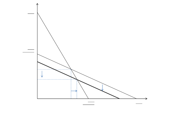
The standard rea
ction functions (8) and (9) are depicted by the thin lines in Chart 1. The intersection
of those lines represents the Nash equilibrium
in the symmetric case. Note that given the
oligopolistic setting, the overall quantity of loans and deposits in the economy will be lower
compared to perfect competition. By slightly reducing the quantity of loans and deposits banks S and
R can keep the rates on bank loans higher while those on deposits lower than under perfect
competition. This allows banks to extract some of the consumer surplus, a standard result in this type
of model.
Chart 1: Loan supply reaction functions in the symmetric case and in the presence of funding
impairments
We now turn to the
asymmetric case. We assume that bank S is perceived to be safe, while bank R is
perceived to be risky. As a result, depositors require an extra compensation of to fund bank R. The
premium reflects the perceived probability of default of that bank. Bank R’s profit maximization
problem is the following:
max
,
= (
(
+
)
)
(
1 +
)
(+ (
+
))
(10)
s.t.:
=
L
S
L
R
+
2
2
L
R
(L
S
)
L
S
(L
R
)
L
R
(L
S
)’
L
R
symmetric case
L
R
funding
impairment case
L
S
symmetric case
L
S
funding
impairment case
Δ
½ Δ
E
0
E
1
+
2
+
2
2
+
2
ECB Working Paper Series No 2364 / January 2020
13

The solution of the above maximisation program, co
mbined with the balance sheet identity for the
safe bank
=
, yields bank R’s reaction function to bank S’s loan supply decision
(
)
in the
case of a funding impairment:
=
(11)
The risk premium required by investors translates into higher marginal funding costs for bank R and
as result its overall supply of loans declines irrespective of the volume of loans provided by its
competitor S. This leads to a parallel downward shift in bank’s R reaction function, as depicted by the
thick line in Chart 1. The intersection between the new reaction function of bank R,
(
)
, and the
reaction function of bank S,
(
), represents the new Nash equilibrium
. The comparison of the
two equilibria
and
yields two main insights. First, the funding impairment of the risky bank
leads to a decline in its supply of bank loans. Second, overall credit supply is also lower, as the supply
of loans by the safe bank compensates for only half of the missing lending by its competitor (see
equation 8).
We now turn to the impact of TLTROs on the equilibrium in the loan market. We will show that the
introduction of the TLTROs affects the loan supply of both banks even if only one of them actually
bids in the operation, as the TLTROs have both direct and indirect effects. In particular, assume that
banks can fund up to a fraction of their loan portfolio with TLTROs at an exogenous interest rate .
We assume that the central banks sets equal to deposit rate paid by the safe bank. In addition, we
assume that bidding in the TLTRO entails additional, small fixed administrative costs.
13
In this set-up,
the safe bank will abstain from bidding since it does not benefit from a funding cost reduction and
avoids the administrative costs. By contrast, given the price attractiveness of the TLTRO funding, the
risky bank will exhaust its borrowing limit, so that =
. The balance sheet identity of the
risky bank includes now TLTROs in addition to deposit funding:
=
+ . The combination
of these two equations yields the new constraint,
(
1
)
=
, which indicates that the risky
bank only funds a proportion 1 of their loan portfolio with deposits. The new maximisation
problem of the risky bank is the following:
max
,
= (
(
+
)
)
(
1 +
)
+
(
+
)
(12)
13
These fixed administrative costs could be the reporting requirements and additional audit obligation that are
a pre-requisite for the access to the TLTROs.
ECB Working Paper Series No 2364 / January 2020
14

s.t.:
(
1
)
=
and =
.
The solution of the above maximisation program, combined with the balance sheet identity of the
safe bank
=
, yields bank R’s reaction function in the case of funding impairments after the
introduction of TLTROs
(
)
:
=
+
()
(
)
(13)
=
1
1
1 +
+
(
1
)
(
+
)
+
(1 )
1
1 +
+
(
1
)
(+
(
1
)
)
Finally, note that the maximisation problem of bank S remains unchanged after the introduction of
TLTRO. However, the shadow price of extending an additional unit of loans – in our case the marginal
costs of deposit funding – for the safe bank changes. Since the risky bank substitutes deposits with
TLTROs the competition in the deposit market weakens, providing a boost to the supply of loans by
bank S. Mechanically, this effect is taken into account by considering the new balance sheet identity
of the risky bank (
(
1
)
=
) when obtaining bank S’ loan supply reaction function. The new
reaction function of the safe bank is the following:
=
(
)
(14)
The comparison of equations (8) and (14) reveals that the safe bank’s loan supply is now less
sensitive to changes in the supply of loans by the risky bank. This is illustrated in Chart 2, which
depicts the equilibria in the loan market before the introduction of the TLTROs (
) and following the
implementation of the TLTROs (
). The reaction functions of both banks shift. The reaction function
of the safe bank becomes steeper, while the intercept with the horizontal
axis remains
unchanged. In the case of the risky bank, both the slope and the intercept change, as the reaction
function steepens and shifts upwards: given that the risky bank receives a significant funding cost
relief due to the TLTROs, its supply of loans increases for any given value of loans granted by the safe
bank. The new Nash equilibrium in the illustration is
, which in the example features higher loan
supply by both banks. While lending by the risky bank always increases in equilibrium, for the safe
bank it very much depends on the exact parameter values, in particular on the shape of the loan
demand and deposit supply functions (a and c), the fraction of bank loans that can be funded with
TLTROs () and the exact TLTRO rate ().
ECB Working Paper Series No 2364 / January 2020
15
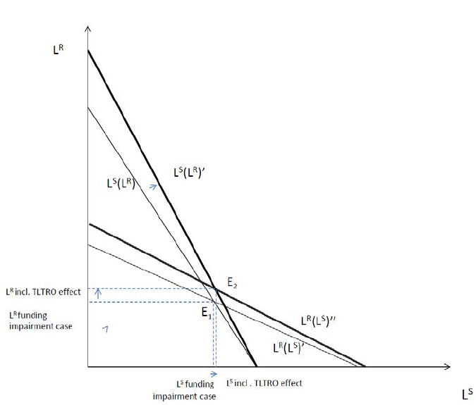
Chart 2: Loan supply reaction functions in the presence of funding impairments before and after the
introduction of a TLTRO
To put it differently, the impact on the loan supply by the safe bank is ambiguous because there are
two opp
osite effects. On the one hand, the TLTROs reduce the marginal costs of its competitor, the
risky bank, which expands its loan supply. Thereby the TLTROs promote stronger competition in the
credit market. Since the banks compete à la Cournot, loan quantities are strategic substitutes,
implying that an increase in the loan supply of the risky bank leads to a contraction in the loan supply
of the safe bank. On the other hand, the TLTROs lead to weaker competition in the deposit market by
the risky bank. As the risky bank substitutes deposits with TLTROs, competition in the deposit market
weakens, which in turn implies lower marginal funding costs for the safe bank, which boosts its loan
supply.
The upshot of the theoretical discussion is that the TLTROs may have important indirect effects on
the credit supply of non-participating banks, as measured empirically by credit standards and loan
margins. In particular, the TLTROs may have important funding externalities on non-bidding banks,
which are not necessarily restricted to retail funding. For instance, as the TLTROs allow participating
ECB Working Paper Series No 2364 / January 2020
16

banks to replace market-bas
ed bank funding with borrowing from the central bank, they can result in
a reduction in the supply of bank bonds in the economy. The scarcity of bank bond issuance should
translate into lower yields on bank bonds, including those issued by intermediaries not participating
in the TLTROs. In addition, the TLTROs may foster competition in the credit market by reducing the
marginal funding costs of participating banks, which allows them to expand their credit supply. Non-
participating banks may react by contracting their loan supply or by expanding their loan supply
depending on which effect dominates: a) the improved market position of competitors that borrow
from the TLTROs, which benefit from a direct funding costs reduction and are therefore able to (re-)
gain market shares at the expense of non-participants or (b) the indirect funding costs relief enjoyed
by bidders and non-bidders alike, which supports the supply of bank loans of both. Hence, the overall
impact of the TLTROs on non-participating banks is a priori ambiguous and must be assessed
empirically.
14
5. Identification strategy
Our
main goal is to estimate the impact of the TLTROs o
n banks’ lending policies, as measured by
bank credit standards and margins. There are two main channels. The first channel is direct: by
participating in the TLTROs, a bank may reduce its funding costs and improve its overall liquidity
position. This allows participating banks to relax credit standards, narrow margins and compete more
aggressively. The second channel is indirect and conceptually focuses on the strategic reactions of
banks – irrespective of whether they bid in the operations - to changes in the competitive pressure.
TLTROs may influence a bank’s lending policies through (i) the positive effect on the balance sheets
of its competitors, which increases the competition in the credit market, and (ii) the less tense
competition in important funding markets due to bidders’ recourse to long-term central bank
funding.
We construct two variables to measure those effects. The direct effect is captured with
bank TLTRO
, which is computed as the ratio between the uptake in the initial TLTROs (September
and December 2014) by bank i and its total assets.
15
The indirect effect is captured with
14
Note that demand for bank loans will increase as the lower funding costs of both bidders and non-bidders
results in lower rates charged on bank loans.
15
Using overall take-up instead of the take-up in only the first two TLTRO-I leads to overall very similar
empirical findings but leads to a weaker instrument, in terms of the first-stage regressions.
ECB Working Paper Series No 2364 / January 2020
17

country TLTRO
(
)
, which is the ratio between the sum of the initial TLTRO uptakes of all the other
banks in the country (i.e., excluding bank i) and the total assets of those banks. Formally:
bank TLTRO
=
(15)
country TLTRO
(
)
=
(16)
There are two main specifications. In the first one, we estimate the probability that lending policies
ease (i.e., eased credit standards or narrower margins, Y
= 1) as a function of bank TLTRO
,
country TLTRO
(
)
and a wide set of bank controls, demand controls and macro controls, plus time
dummies. Formally:
Y
= bank TLTRO
+ country TLTRO
(
)
+ X
+ W
+ X
+ d
+
+
(17)
where i is bank, c is c
ountry, t is quarter, Y
is the binary outcome variable (credit standards or
margins), X
is a vector of time-varying bank controls, W
is a vector of demand controls (which
also vary at the bank-quarter level), X
is a vector of time-varying macro controls, d
are time
fixed effects,
is a country-quarter error component and
is an individual error term. The main
coefficient of interest is , which captures the indirect effect of the TLTROs on lending policies.
The second specificatio
n is quite similar to (17), but focuses instead on the direct effect of the
TLTROs. To do so, we drop the variable country TLTRO
(
)
and the macro controls and saturate the
regression with country-time fixed effects (d
). Formally:
Y
= bank TLTRO
+ X
+ W
+ d
+
(18)
The main coefficient of interest is , whi
ch captures the direct effect of the TLTROs on lending
policies.
We estimate (17) and
(18) for the period 2014Q2-2017Q4. Hence, our empirical strategy implies a
comparison of changes in credit standards/margins between treated and non-treated banks (e.g.
high and low country TLTRO
(
)
) after the announcement of the TLTROs in June 2014.
16
We also
perform placebo tests to make sure that any potential differences in the outcome variable across the
16
Note that our dependent variables credit standards and, to a lower extent, loan margins, are quite sticky, i.e.,
they evolve very slowly over time. This means that we must also use the cross-section variation for
identification, which renders the inclusion of bank fixed effects not feasible.
ECB Working Paper Series No 2364 / January 2020
18

two groups of banks were not pres
ent already before the TLTROs and thus can be attributed to the
introduction of the measure.
Estimation of (17) and
(18) by OLS may lead to biased and inconsistent estimates due to selection
bias.
17
In particular, selection into treatment is non-random, as banks participated in the TLTROs on a
voluntary basis. In particular, the evaluation of the policy may be biased upwards if the banks that
borrowed (more) from the TLTRO had, on average, better lending opportunities. By contrast, the
estimates may be biased downwards if the banks that borrowed (more) from the TLTRO had greater
deleveraging needs.
In order to obtain consistent estimates of and w
e use two instrumental variables that come from
the institutional setting of the TLTROs, as in Benetton and Fantino (2017). In particular, as explained
in section 3, in the initial TLTROs-I (September and December 2014) banks could borrow an amount
equivalent to 7% of their eligible loans outstanding on 30 April 2014. Crucially, note that the stock of
eligible loans was measured at prior to the announcement of the policy (June 2014). This initial
allowance constitutes the exogenous component of the TLTRO uptakes, as it is based on exogenous
parameters that are common across banks and on pre-determined banks’ balance sheet
characteristics. By contrast, we disregard the amounts borrowed in the additional TLTROs (between
March 2015 and June 2016) because the additional borrowing allowances depended on the evolution
of banks’ eligible lending activities in excess of bank-specific benchmarks. Hence, both the additional
TLTRO uptakes and their borrowing allowances are clearly endogenous variables.
Therefore, we construct two instrumental variables, bank al
lowance
and country allowance
(
)
.
The first one is computed as the ratio between the initial borrowing allowance of bank i and its total
assets. The second one is constructed as the ratio between the sum of the initial allowance of all the
other banks in the country (i.e., excluding bank i) and the total assets of those banks. Formally:
bank allowance
=
(19)
country allowance
(
)
=
(20)
17
In addition to selection bias, the fact that one regressor, country TLTRO
(
)
, is the average of another,
bank TLTRO
, may complicate the interpretation of OLS estimates of equation (17). See Angrist and Pischke
(2009), pages 193-195, for an explanation.
ECB Working Paper Series No 2364 / January 2020
19

We then estimate (17) a
nd (18) by 2SLS.
18
Note that equation (17) includes the individual TLTRO
uptakes,
, although we are really only interested in the aggregate effect of TLTROs –the
effect of
(
)
- in that specification. The inclusion of
is motivated by
the fact that any instrument for
(
)
must be also correlated with
. By
including it in the regression (as a second endogenous variable) we avoid a violation of the exclusion
restriction.
19
Finally, an additional id
entification challenge is to disentangle shocks to credit supply from shocks to
credit demand, as those shocks are often correlated and what we observe are equilibrium outcomes.
For instance, banks with high TLTRO uptakes may face more dynamic demand conditions or deal with
more creditworthy borrowers, which may induce them to ease credit standards or narrow margins.
To control for demand factors, we include a large vector of control variables that measure the
evolution of credit demand by firms and households in different segments (e.g. loans to SMEs), as
well as the factors underlying those developments (e.g., consumer confidence) as reported by banks
in the BLS.
20
18
Notice that the estimation of (17) via OLS would entail in addition an omitted variables bias from the
correlation between country TLTRO
(
)
and other country-quarter effects embodied in the error component
. For instance, the country’s business cycle may affect the country’s level of TLTRO uptakes because it
determines banks’ lending opportunities and firms’ investment returns and it also affects credit standards and
margins, which are usually anticyclical. This may generate a spurious correlation between the two. While the
inclusion of time-varying macro controls (such as the industrial production index and the unemployment rate)
mitigates this problem, a more complete solution is the approach we follow, IV estimation. By contrast, the
estimation of (18) does not face this challenge, as the use of country-time fixed effects
eliminates this
source of variation.
19
See Acemoglu and Angrist (2000) for a similar identification strategy in the context of the social returns to
schooling and human capital externalities.
20
In the case of non-financial corporations, demand controls are dummy variables for changes (decrease,
unchanged, increase) in the demand of credit in the following segments: all firms, SMEs and large firms, short-
term loans and long-term loans, loans for fixed investment, loans for inventories, loans for mergers and
acquisitions and loans for debt refinancing/restructuring. In the case of housing loans, demand controls are
dummy variables for changes (decrease, unchanged, increase) in the demand of credit by households for house
purchase and changes in the demand due to housing market prospects, consumer confidence, the general level
of interest rates, debt refinancing and the regulatory and fiscal regime of housing markets.
ECB Working Paper Series No 2364 / January 2020
20

Regarding inference, standard errors are clustered at the bank level to allow
for potential
heteroscedasticity and serial correlation within groups in the error structure. Nevertheless, results
are very similar when clustering at a higher level of aggregation such as country.
21
6. Data and variables
The data employed in the baseline analyses come from four s
ources: the Individual Bank
Lending Survey (iBLS), the Individual Balance Sheet Items (IBSI), the Individual MFI Interest Rate
(IMIR) databases and proprietary information on banks’ participation in central bank credit
operations. The iBLS database contains confidential, non-anonymized replies to the ECB’s Bank
Lending Survey (BLS) for a subsample of banks participating in the BLS. The BLS is a quarterly survey
through which euro area banks are asked about developments in their respective credit markets
since 2003.
22
Currently the sample comprises more than 140 banks from 19 euro area countries and
covers around 60% of the amount outstanding of loans to the private non-financial sector in the euro
area. However, there are six countries that do not share the confidential, non-anonymized replies to
the BLS so they do not participate in iBLS (see Table 1 for a view of the distribution of observations
per country).
23
The BLS is specifically designed to distinguish between supply and demand conditions in the
euro area credit markets. Supply conditions are measured through credit standards (i.e., the internal
guidelines or loan approval criteria of a bank) and credit terms and conditions (loan margins, loan
size, loan maturity, etc).
24
The BLS also contains information on the evolution of credit demand by
21
While clustering at the country level may lead to standard errors that are biased downwards due to few
clusters (Bertrand et al. 2004), inference using wild cluster bootstrap, a solution developed by Cameron et al.
(2008), leads to qualitatively similar results.
22
For more detailed information about the survey see Köhler-Ulbrich, Hempell and Scopel (2016). Visit also
https://www.ecb.europa.eu/stats/ecb_surveys/ban
k_lending_survey/html/index.en.html.
23
Germany participates in the iBLS with a sub-sample of banks that have agreed to transmit their non-
anonymized replies to the ECB.
24
According to the BLS, credit standards are the internal guidelines or loan approval criteria of a bank. They are
established prior to the actual loan negotiation on the terms and conditions and the actual loan
approval/rejection decision. They define the types of loan a bank considers desirable and undesirable, the
designated sectoral or geographic priorities, the collateral deemed acceptable and unacceptable, etc. Credit
standards specify the required borrower characteristics (e.g., balance sheet conditions, income situation, age,
employment status) under which a loan can be obtained. On the other side, credit terms and conditions refer
to the conditions of a loan that a bank is willing to grant, i.e., to the terms and conditions of the individual loan
actually approved as laid down in the loan contract which was agreed between the bank and the borrower.
They generally consist of the agreed spread over the relevant reference rate, the size of the loan, the access
ECB Working Paper Series No 2364 / January 2020
21

firms and households and the factors underlying these developments. In addition, several ad hoc
que
stions have been added in the recent years to analyse the impact of the main non-standard
monetary policy measures introduced by the ECB, such as the negative deposit facility rate (DFR) or
the expanded asset purchase programme (APP), on several dimensions such as banks’ balance
sheets, credit standards and terms and conditions.
IBSI and IMIR contain balance-sheet and interest rate information of the 326 largest euro
area banks
,
25
which is individually transmitted on a monthly basis from the national central banks to
the ECB since July 2007. We have matched both datasets with the iBLS and information on banks’
participation in Eurosystem credit operations, among which importantly the TLTROs. We restrict the
sample to the period spanning from 2014Q2 (i.e., announcement of TLTRO-I) to 2017Q4
.
26
The
resulting sample contains 1,784 observations corresponding to an unbalanced panel of 130 banks
from 13 countries (see Table 1 for a view of the distribution of observations per country).
27
However,
the estimation sample will be generally smaller due to missing values.
The definitions of the variables used in this study are displayed in Table 2. The dependent
variables are changes in credit standards and margins in loans to enterprises and households for
house purchase, as reported in the BLS. In particular, the BLS asks banks on a quarterly basis about
the evolution of the credit standards applied to their new loans or credit lines to enterprises and
households, as well as the margins charged on them. Banks must answer whether they have
tightened credit standards, kept them basically unchanged or eased them over the past three
months.
28
Regarding margins (defined as the spread over a relevant market reference rate), the BLS
distinguishes between margins on average loans and margins on riskier loans. Banks must answer
conditions and other terms and conditions in the form of non-interest rate charges (i.e., fees), collateral or
guarantees which the respective borrower needs to provide (including compensating balances), loan covenants
and the agreed loan maturity.
25
55 monthly time series are required on the asset side, which include data on holdings of cash, loans, debt
securities, MMF shares/units, equity and non-MMF investment fund shares/units, non-financial assets and
remaining assets. On the liability side, the time series cover information on deposits, included and not included
in M3, issuance of debt securities, capital and reserves and remaining liabilities.
26
As most regressors are lagged one period, they are measured in the period spanning 2014Q1 to 2017Q2.
27
The level of consolidation of the banking group differs between BLS and IBSI. Consequently, we have 130
banks in IBSI but 112 banks in BLS, because sometimes the head of the group is the one that answers to the BLS
but we have unconsolidated balance sheets of the head and its subsidiaries in IBSI.
28
While the BLS differentiates between “tightened considerably” and “tightened somewhat” and between
“eased considerably” and “eased somewhat”, we aggregate these categories into “tightened” and “eased”, as
done in the regular BLS reports prepared by the ECB.
ECB Working Paper Series No 2364 / January 2020
22

whether they have tightened them (wid
er margins), kept them basically unchanged or eased
(narrower margins) over the past three months.
Descriptive statistics of the dependent variables can be found in Table 3
. They are dummy variables
that equal 1 in the case of easing and 0 otherwise. Credit standards are very stable over time. The
proportion of banks that report an easing of credit standards ranges between 5% and 7%, depending
on the segment. Margins on average loans ease more frequently, in about 25% of the observations,
while margins on riskier loans are narrowed less often (about 5%). Therefore, while banks adapt their
lending policies through the adjustment of both loan terms & conditions and credit standards, the
former seem to be more flexible instruments than the latter. Regarding bank-level controls, we proxy
bank size with the natural logarithm of the bank’s total assets (size). Leverage is defined as the ratio
of capital and reserves over total unweighted assets (capital ratio). Liquidity is measured with a
liquidity ratio, expressed as the sum of cash, holdings of government securities and Eurosystem
deposits over total assets (%). This variable may also capture the impact of the ECB’s expanded asset
purchase programme (APP) on banks’ balance sheets, which was announced in January 2015. We
also include a loan-to-deposit ratio, in logs.
29
The importance of deposits as a funding source is
captured with the deposit ratio, the ratio between the deposits by households and non-financial
corporations over total assets. Market share is the ratio between a bank's outstanding loans and the
total loans of the country's banking sector (%). We also control for the bank’s legal form (head
institution, national subsidiary, foreign subsidiary, foreign branch). Finally, we need to control for the
impact of negative interest rates on banks’ lending policies because both the TLTRO I and the
negative deposit facility rate (DFR) were announced in June 2014, as part of the ECB’s credit easing
package.
30
To do so we include the variable NDFR, a dummy variable that equals 1 if the bank
reported that the ECB’s negative DFR contributed to a decrease of the bank’s net interest income in
the past six months and 0 otherwise. This variable, which comes from Arce et al. (2018), is
constructed using an ad-hoc question in the BLS that is asked on a semi-annual basis.
31
We also
include a set of relevant macroeconomic controls: the 10-year sovereign bond, the industrial
production index, the unemployment rate, the consumer price index and the Herfindahl-Hirschman
Index.
29
To correct for right skewness and outliers.
30
The negative DFR was introduced on 11 June 2014, the TLTRO-I were announced on 5 June 2014.
31
The exact wording of the question is: “Given the ECB’s negative deposit facility rate, did this measure, either
directly or indirectly, contribute to a decrease / increase of your bank’s net interest income over the past six
months?”
ECB Working Paper Series No 2364 / January 2020
23

Table 4 displays descriptive statistics of the bank characteristics, including the key
re
gressors, the instrumental variables and the bank-level controls, as well as summary statistics of
the macro controls. Table 5 presents the means of the bank characteristics for banks that
participated in the TLTROs and banks that did not participate, together with the p-value associated
with a two-sample t-test of equality of means, at the quarter of announcement of TLTRO-I (2014Q2).
Out of the 116 banks in the sample at 2014Q2, 55 banks participated in the TLTRO.
32
The average
participating bank borrowed an amount equivalent to 1.7% of its total assets (mean of
bank TLTRO
), close to its borrowing limit, 2% (mean of bank allowance
). Regarding differences
between bidders and non-bidders, the average TLTRO uptake of a bank’s competitors (mean of
(
)
) is higher in the case of participating banks. This likely reflects that banks located
in countries under intense financial market scrutiny during the sovereign crisis episode participated
more widely and borrowed larger amounts. This is not surprising since the funding cost benefit of
accessing the TLTROs, instead of alternative funding, was on average higher for banks located in
those countries. To some extent it may also reflect that the recourse to the operations are strategic
complements: a bank is more likely to participate if its rivals borrow heavily in the operations. In
addition, TLTRO bidders are significantly larger than non-bidders, probably due to the fixed costs
associated with participation, and have a larger market share in the segment of loans to NFCs. With
respect to risk, there are no significant differences in terms of capital and non-performing loan ratios,
but bidders have higher CDS spreads than non-bidders, suggesting that they are perceived to be
riskier. However, this last result must be interpreted with caution, as we only have information on
CDS spreads for 83 banks. Participating banks also have a substantially higher share of liquid assets,
probably because some of those assets can be pledged as collateral in the TLTROs and the ECB’s main
refinancing operations. Bidders are also more likely to experience a decline in their net interest
income due to negative interest rates (NDFR=1) than non-bidders.
In our empirical exercises we also use controls for firms’ demand for credit. In particular, the
BLS asks banks about perceived changes in the demand for loans or credit lines to enterprises and
households. Banks must answer whether the demand for their loans has decreased, has remained
basically unchanged or has increased over the past three months.
33
In the case of loans to non-
32
Note that we have an unbalanced panel. Out of 130 banks in the whole sample (2014Q2-2017Q4), 60 of
them participated in the initial TLTROs.
33
As with the supply indicators, we merge “decreased considerably” and “decreased somewhat” into
“decreased” and “increased considerably” and “increased somewhat” into “increased”.
ECB Working Paper Series No 2364 / January 2020
24

financial corporations, we d
ifferentiate between demand for loans from SMEs and large firms and
also between short-term loans and long-term loans. We also distinguish the evolution of credit
demand according to the purpose of the loan (loans for fixed investment, for inventories and working
capital, for mergers and acquisitions and for debt refinancing). In the case of loans to households for
house purchase, we include dummy variables for changes in the demand of credit in that segment, as
well as changes in the demand due to the factors “housing market prospects” and “consumer
confidence”.
34
Table 6 presents descriptive statistics of these variables. The demand indicators are
also relatively stable, but they change more frequently than credit standards. In addition, demand is
more likely to increase than to decrease, as expected in a period of economic recovery.
Descriptive analyses suggest a meaningful relationship between the dependent variables and
the key regressors. For the segment of loans to NFCs, Figure 2 displays the averages of the
dependent variables (i.e., the proportion of banks that eased credit standards/margins) for banks
with high/low values of
(
)
(above and below the median, respectively). According
to Figure 2, banks that belong to the high country TLTRO group are more likely to ease credit
standards and margins on average loans than banks that belong to the low country TLTRO. The
differences are sizeable and statistically significant.
35
For instance, the proportion of banks that
eased overall credit standards was 8% for the high country TLTRO group and only 3% for the low
country TLTRO group. By contrast, banks whose national competitors borrowed heavily in the TLTROs
(high country TLTRO group) were less likely to narrow margins on riskier loans than banks from the
low country TLTRO group (5% and 8%, respectively). A similar analysis is displayed in Figure 3 for
banks with high/low values of bank TLTRO
(above and below the median).
36
According to Figure 3,
banks with high TLTRO uptakes were more likely to ease credit standards and margins on average
loans than banks with low uptakes. The differences are also statistically significant, although
somewhat smaller than in Figure 2. By contrast, the proportion of banks that narrowed margins on
riskier loans is very similar in both groups. All in all, the analysis of the two figures suggests
potentially meaningful links between TLTRO uptakes at the bank and country level and changes in
34
Similarly to the case of supply factors (e.g. competition), a demand factor may contribute to lower demand,
to keeping demand unchanged and to higher demand. We exclude other BLS demand factors (general level of
interest rates, debt refinancing/restructuring and regulatory and fiscal regime of housing markets) because
there are only available since 2015Q1 due a change in the questionnaire.
35
The statistical significance of those differences is assessed by performing two-sample tests on the equality of
proportions.
36
As the median of bank TLTRO
is 0, the two groups consist of participating and non-participating banks.
ECB Working Paper Series No 2364 / January 2020
25

banks’ lending policies. However, as these associations may be purely due to positive selection bias
(e.
g. banks with high TLTRO uptakes may have better lending opportunities) or confounding events
(e.g. those banks may have been more affected by the negative DFR that was introduced in parallel),
more formal analyses are required.
7. Empirical results
7.1 Baseline res
ults
Let us start with the segment of loans t
o NFCs. As a benchmark, Table 7a and Table 7b
display the estimation of (17) and (18) by OLS. Table 7a shows that there is a positive and significant
correlation between the TLTRO uptakes of a bank’s national competitors, as measured by
country TLTRO
(
)
, and the probability that the bank eases overall credit standards (column (1)),
credit standards to SMEs (column (2)) and credit standards to large firms (column (3)). This suggests a
significant indirect effect of the TLTROs on bank credit standards. By contrast, there is no significant
impact on bank margins (columns (4) and (5)). In addition, Table 7b shows no clear evidence of direct
effects, as a bank’s TLTRO uptake is not significantly correlated with the probability of easing credit
standards or lowering margins. The only exception is column (5), which displays a negative sign:
higher TLTRO uptakes are associated with a lower probability of narrowing margins on riskier loans.
This observation may indicate that the TLTROs did not lead to excessive risk taking by banks.
To make sure that our results are not biased by en
dogeneity we use the initial TLTRO-I
allowance (at bank and country level respectively) as instrument variables and estimate (17) and (18)
by 2SLS.
37
First we confirm that the instruments are not weak. Table 8 reports the first stage
regressions corresponding to (17) (columns (1) and (2)) and the first stage regression that
corresponds to (18) (column (3)). We observe positive and strong relationships between the
instruments and the endogenous variables. In particular, a 1 pp increase in a bank’s initial allowance
leads to a 0.49 pp increase in a bank’s TLTRO uptake (over total assets), and a 1 pp increase in a
country’s initial allowance leads to a 0.59 pp increase in a country’s total TLTRO uptake (over the
country’s total assets). In columns (1) and (2), the multivariate F-statistics developed by Sanderson
37
In a supplement to this paper we report estimates of (17) by probit and IV probit. Results are broadly similar.
ECB Working Paper Series No 2364 / January 2020
26

and Windmeijer (2016)
38
exceed Stock and Yogo (2005)’s critical values
39
and they are significantly
greater than 10, the rule of thumb suggested by Staiger and Stock (1997). The same is true for a
conventional first-stage F-statistic in column (3). Hence, we can conclude that our instruments are
not weak.
The 2SLS estimates, which are presented in Table 9,
are consistent with the previous OLS
results. Regarding indirect effects (Table 9a), country TLTRO
(
)
has a positive effect on overall
credit standards, credit standards for SMEs and credit standards for large firms (columns (1), (2) and
(3)). The effects are sizeable. For instance, a standard deviation increase in country TLTRO
(
)
leads
to a 5.3 pp increase in the probability that a bank eases overall credit standards and an 8.8 pp
increase in the probability of easing credit standards to large firms. By contrast, the TLTRO uptakes of
a bank’s competitors have no significant effect on margins on average loans (column (4)) and riskier
loans (column (5), coefficient only marginally significant). Finally, there is no clear evidence of direct
effects (Table 9b), as the coefficient on bank TLTRO
is insignificant in all specifications.
The analysis of loans to hous
eholds for house purchase is presented in Table 10 (OLS) and
Table 11 (2SLS). For the sake of brevity, let us focus on the IV estimates. With respect to indirect
effects (Table 11a), country TLTRO
(
)
has a positive effect on credit standards (column 1). In
particular, a standard deviation increase in the TLTRO uptakes of a bank’s competitors implies an 8.8
pp increase in the probability that the bank eases its own credit standards. Regarding direct effects
(Table 11b), there is no significant impact on credit standards (column 1). However, column (2)
reports a positive effect of bank TLTRO
on the probability of narrowing margins on average loans.
The effect is strong, as a standard deviation increase in a bank’s TLTRO uptake (relative to total
assets) implies a 15.8 pp increase in the probability of lowering margins on average loans.
7.2 Analysis of the direct effects of the TLTROs: the intensive vs. extensive margin
The evidence presented so far suggests that direct effects are weak, except in the case of
margins on loans for house purchase. However, notice that the regressor of interest,
,
38
For multiple endogenous variables, inspection of the individual first-stage F-statistics is not sufficient. To see
why, suppose there are two instruments for two endogenous variables and that the first instrument is strong
and predicts both endogenous variables well, while the second instrument is weak. The first-stage F-statistics in
each of the two first-stage equations are likely to be high, but the model is weakly identified, because one
instrument is not enough to capture two causal effects. See Angrist and Pischke (2009).
39
For a Wald test with maximal size of 10%.
ECB Working Paper Series No 2364 / January 2020
27
may hide some interesting heterogeneity. In particular, the variable takes the value 0 for about 50%
of the observations (banks that did not borrow in the TLTROs) and it is continuously distributed
between the values 0.1% and 5% for the other 50% of the observations (banks that borrowed in the
TLTROs). Hence, we may distinguish the direct effect of TLTROs on bank lending policies in the
extensive margin (participation vs. non-participation) and the intensive margin (amount of borrowed
funds, conditional on participation). For the analysis of the extensive margin, we estimate (18) but
replacing the variable
with the variable
, a dummy that equals 1 the
bank borrowed any amount in the initial TLTROs (September and December 2014). We treat
as endogenous and instrument it with bank allowance
. For the analysis of the
intensive margin, we estimate (18) for the subsample of banks that participated in the initial TLTROs.
The analysis for the segment of loans to NFCs is presented in Table 12. Table 12a examines
the intensive margin and Table 12b examines the extensive margin. According to Table 12a, there are
no substantial differences in the lending policies of participating and non-participating banks, as the
coefficient on
is always statistically insignificant. In other words, there is no
“participation effect”. By contrast, for the subsample of bidding banks (Table 12b), the coefficient on
is positive and significant in columns (3) and (4), indicating that high TLTRO uptakes
lead to a higher probability of easing credit standards on large firms and to a higher probability of
narrowing margins on average loans. The effects are strong: a standard deviation increase in a bank’s
TLTRO uptake increases the probability of easing credit standards on large firms by 12.4 pp and it
raises the probability of narrowing margins on average loans by 20 pp. This suggests that, for the
subsample of bidding banks, the reduction in funding costs caused by the TLTROs is transmitted
through easier lending policies to large firms and relatively safe borrowers.
The analysis for the segments of loans to households is presented in Table 13. Table 13a
examines the intensive margin and Table 13b examines the extensive margin. According to Table
13a, bidding banks are much more likely (62 pp) to narrow margins on average loans than non-
bidders, a strong “participation effect”. The effect on those margins also takes place in the intensive
margin (Table 13b): for the subsample of bidding banks, a standard deviation increase in a bank’s
TLTRO uptake raises the probability of narrowing margins on average loans by 28.6 pp. All in all, the
picture that emerges from Tables 9, 11, 12 and 13 is that there are substantial direct effects of
TLTROs on lending policies. The direct transmission of monetary policy takes place mainly through
the adjustment of margins on loans to relatively safe borrowers.
ECB Working Paper Series No 2364 / January 2020
28

7.3 Further analysis of indirect effects: the role of competition
The evidence presented so far suggests that the TLTROs have important indirect effects on
banks’ lending policies. Recall that, according to the above stylised model, large-scale recourse to the
TLTROs has two simultaneous effects: (i) it fosters intense competition in the credit market and (ii) it
eases pressures in funding markets. While for bidders (i.e., the risky bank) these two effects go in the
same direction,
40
for non-bidders (i.e., the safe bank) the effects are opposite. On the one hand their
relative competitive position vis-à-vis bidders worsens, ceteris paribus contracting the loan supply of
non-bidders. On the other hand, their access to market funding improves, supporting their supply of
loans. The empirical results presented so far suggest that the overall indirect effect is positive, i.e.
that the overall easier access to market funding for non-bidders more than compensates for their
lost competitive position vis-à-vis bidders.
Against this background we try to isolate the positive indirect impact of the TLTROs on the
loan supply of non-bidders via the positive funding externalities. We do this by controlling for the
intensity of competition in credit markets, as reported by banks in the BLS. In particular, the BLS asks
banks about the evolution of several factors that affect their credit standards and their terms and
conditions. Specifically, a factor may contribute to a tightening of credit standards (terms &
conditions), to keeping credit standards (terms & conditions) unchanged or to an easing of credit
standards (terms & conditions). In this section we use the variable competition, which equals 1 if the
factor "pressure from competition" contributed to an easing of terms and conditions, and 0 if it was
unchanged or contributed to a tightening.
41
The results of this exercise are presented in Table 14 and 15. Note that in this set-up the
coefficient on country TLTRO
(
)
only captures the positive funding externality of those operations.
As expected, the respective coefficients are positive and significant when the dependent variables
are credit standards (columns 1-3 of Table 14 and column 1 of Table 15). The effects are also
40
Access to the TLTROs levels the playing field from their perspective and results in an overall improved
competitive position vis-à-vis non-bidders. And on top of that, the interest rates on deposits decline as a
substitute for market funding is introduced.
41
Similar results are found when we use the variable competition (credit standards), which equals 1 if the
factor "competition from other banks" contributed to an easing of credit standards and 0 if it was unchanged
or contributed to a tightening.
ECB Working Paper Series No 2364 / January 2020
29
sizeable. For instance, a standard deviation increase in country TL
TRO
(
)
leads to a 6.5 pp increase
in the probability that a bank eases overall credit standards to NFCs and to a 7.3 pp increase in the
probability of easing credit standards to households for house purchase. Therefore, the available
evidence suggests that the TLTROs generate significant positive funding externalities, as non-bidders
may benefit from weaker competition in the deposit and bond markets. Note that the coefficients on
competition are positive and significant: an increase in competition leads to a higher probability of
eased credit standards and narrow margins.
We also go on to tes
t whether the overall indirect effects of the TLTROs are stronger in more
competitive environments. Then we estimate equation (17) by 2SLS in subsamples of observations
for which competition equals 1 and 0 (high and low competitive pressures, respectively). Results are
displayed in Tables 16 (loans to NFCs) and 17 (housing loans). In the case of loans to NFCs (Table 16),
the indirect effect of the TLTROs on credit standards is very strong for banks facing high competitive
pressures (columns 1 to 3, Table 16a). For instance, a standard deviation increase in
country TLTRO
(
)
raises the probability of easing overall credit standards by 21 pp. In addition, an
increase in the uptakes of a bank’s competitors reduces the probability of narrowing margins on
riskier loans, suggesting that the TLTROs did not translate into excessive risk taking (column 5, Table
16a). By contrast, those effects are virtually non-existent for banks facing low competitive pressures
(Table 16b). In the segment of loans to households for house purchase (Table 17), the impact of
country TLTRO
(
)
on credit standards is significant in both subsamples, but much larger (7 times) in
the case of high competitive pressures.
Alternatively, we test this
hypothesis in Tables 18 and 19, which report 2SLS estimates of
equation (17) in subsamples of banks with high and low market share (above and below the median,
respectively). In Table 18 (loans to NFCs) we can observe that the impact of country TLTRO
(
)
on
credit standards is particularly high for banks with a low market share (Table 18a, columns 1to 3). For
instance, a standard deviation increase in country TLTRO
(
)
is associated with a 14.4 pp increase in
the probability of easing overall credit standards. By contrast, in the sample of banks with high
market share (Table 18b), the effect is only significant in the segment of large firms (column (3)), and
even in this case it is substantially smaller. Similarly, in Table 19 (loans to households for house
purchase) we observe a very strong effect in the case of banks with a low market share: a standard
deviation increase in country TLTRO
(
)
raises the probability of easing credit standards by 17.7 pp
(column 1, Table 19a). However, the effect is much smaller, and only marginally significant, in the
ECB Working Paper Series No 2364 / January 2020
30

subsample of banks with high market share (co
lumn 1, Table 19b). In addition, an increase in the
TLTRO uptakes of a bank’s competitors leads to a lower probability of narrowing margins on riskier
loans in the case of banks with low market shares (column 3, Table 19a). These findings suggest that
the indirect effects of the TLTROs are particularly strong in the case of banks that face strong
competition in the credit market, as proxied by low market shares.
8. Robustness tests
A stan
dard concern in policy evaluation is the presenc
e of pre-existing trends. If, for some reason,
the evolution of treatment and control groups was not parallel before the implementation of the
policy, the estimates may pick up such behaviour, rather than the causal impact of the policy. In our
empirical implementation, our treatment groups, banks with high TLTRO uptakes and banks whose
national competitors borrowed heavily in the TLTROs, could have started easing credit
standards/margins well before the announcement of the TLTROs in June 2014.
In order to rule out such concerns, w
e carry out a falsification test. In particular, we estimate
equations (14) and (15) by 2SLS for a placebo period spanning from 2010Q2-2014Q1. The placebo
period is as long as the “true period” (2014Q2-2017Q4) and ends right before the announcement of
the TLTROs. In other words, we assume that banks borrowed from the TLTROs in June 2010 and we
observe their lending behaviour in the following 19 quarters.
Results of the falsification tests are presented in Tables 20 (loa
ns to NFCs) and 21 (housing loans).
Regarding the impact of country TLTRO
(
)
on credit standards (Table 20a and 21a), the coefficients
on the variable are no longer statistically significant or -in the case of credit standards on loans to
SMEs- even negative and significant. With respect to the impact of bank TLTRO
, the coefficients are
generally insignificant (Table 20b and 21b). These results suggest that our main findings are not
driven by pre-existing trends.
Another concern regarding the previous empirical analysis is that we may pick up the effect of the
second series of targeted longer-term refinancing operations (TLTRO II) that were implemented
between June 2016 and March 2017. In the case of TLTRO II (announced on March 2016
42
), banks
were able to borrow a total amount of up to 30% of their eligible loans outstanding at 31 January
42
Press release: https://www.ecb.europa.eu/press/pr/date/2016/html/pr160310_1.en.html
ECB Working Paper Series No 2364 / January 2020
31

2016.
43
Incentives for banks to lend to the non-financial private sector were provided via reduction in
the interest rate applied in the operations.
44
The uptakes in TLTRO-I and TLTRO-II are likely to be
correlated, as participating banks used part of the funds to roll over expiring debts. To address this
concern, we estimate (14) and (15) by 2SLS for the shorter period 2014Q2-2016Q1, i.e., before the
implementation of TLTRO-II.
The results are presented in Tables 22 and 23
. They are very similar to the baseline results (Tables 9
and 11). In the case of loans to NFCs, the indirect impact of TLTROs on credit standards becomes
larger (Table 22a). For instance, a standard deviation increase in country TLTRO
(
)
leads to a 6.8 pp
increase in the probability that a bank eases overall credit standards and a 10.4 pp increase in the
probability of easing credit standards to large firms. Interestingly, the negative impact of
country TLTRO
(
)
on the probability of narrowing margins on riskier loans also becomes stronger
and more significant. In particular, a standard deviation increase in country TLTRO
(
)
reduces by
8.7 pp the probability that the bank narrows margins on riskier loans. As before, the direct impact of
TLTROs on credit standards and margins is not significantly different from zero (Table 22b). Things
also change little in the case of housing loans, as there is still a significant impact of
country TLTRO
(
)
on credit standards (Table 23a) and a significant impact of bank TLTRO
on
margins on average loans (Table 23b). Those effects are also larger than in the baseline estimations.
Note that the theoretical framework presented in Section 4 models credit supply in terms of loan
quan
tities, while the empirical analysis proxies credit supply with credit standards and loan margins.
While credit standards are a reliable proxy for credit supply according to previous literature (e.g.
Lown and Morgan (2006) and Ciccarelli et al. (2015)), for robustness we replace them by credit
growth rates
45
in equations (17) and (18). Results are presented in Table 24, which again
distinguishes between indirect effects (Table 24a) and direct effects (Table 24b) for loans to NFCS
(column 1) and loans to households for house purchase (column 2). The coefficient on
43
In particular, 30% of their eligible loans less any amount which was previously borrowed and was still
outstanding under the first two TLTRO operations conducted in 2014.
44
The interest rate applied to TLTRO II was fixed for each operation at the rate applied in the main refinancing
operations (MROs) prevailing at the time of allotment. In addition, counterparties whose eligible net lending in
the period between 1 February 2016 and 31 January 2018 exceeded their benchmark were charged a lower
rate for the entire term of the operation. See ECB press release for details:
https://www.ecb.europa.eu/press/pr/date/2016/html/pr160310_1.en.html
45
Computed as quarterly changes in the natural log of the stock of loans. They are windsorised at 90% to
reduce the impact of outliers.
ECB Working Paper Series No 2364 / January 2020
32
country TLTRO
(
)
is positive and statistically significant in both segments, indicating that a higher
TLTRO uptake by a bank’s national competitors leads to higher credit growth. In particular, a
standard deviation increase in country TLTRO
(
)
causes credit growth to increase by 0.8 percentage
points in each segment. By contrast, there is no evidence of direct effects, as the coefficients on
bank TLTRO
are not statistically different from zero.
Finally, an implic
it assumption of the whole analysis of indirect effects is that European credit and
funding markets are segmented at the national level, probably due to a large array of regulatory,
technological and cultural factors (e.g. different languages). In this context, each bank is influenced
by the behaviour of its national competitors, as captured by the variable country TLTRO
(
)
.
However, this may not be true in the case of very large well-diversified banks that simultaneously
compete in many European markets. To ameliorate this concern, we take out from the sample those
banks classified as globally systemic banks (G-SIB) by the Financial Stability Board. These banks have
many similarities: they are very large, are all conglomerates, have an international geographical
orientation and tend to be diversified (Altavilla et. al 2018b). We then re-run regressions (17) and
(18). The results, displayed in tables 25 and 26, are very similar to the baselines estimates: significant
indirect effects on credit standards in both segments and significant direct effects on margins on
average loans to households for house purchase.
9. Conclusions
This
paper assesses the impact of the Eurosystem’s Target
ed Long-Term Refinancing Operations
(TLTROs), announced in June 2014, on the lending policies of euro area banks. To guide our empirical
researc
h, we first present a simple model of oligopolistic competition in the banking sector in which
two banks compete à la Cournot in the loan and deposit markets. One of the banks, with high
funding costs, participates in the TLTROs, while the other one, with low funding costs, does not. The
model helps us distinguish between the direct and the indirect effects of the TLTROs. Regarding
direct effects, the TLTROs reduce the marginal costs of the participating bank, which expands its
credit supply. There are two indirect effects. First, the TLTROs increase the competition in the credit
market by levelling the playing field. Second, as the bidder replaces part of deposit funding with
TLTRO funding, the competition in the deposit market weakens, which reduces deposit rates and the
marginal costs of the non-bidder. The main predictions of the model are a positive direct impact of
ECB Working Paper Series No 2364 / January 2020
33
the TLTRO on the bidder’s credit supply and an ambiguous indirect impact on the non-bid
der’s loan
supply.
We then test those predictions with the c
onfidential answers to the ECB’s Bank Lending Survey (BLS)
by 130 banks from 13 euro area countries, matched with individual bank balance-sheet information
and operations data. We measure bank lending policies with credit standards (i.e., the internal
guidelines or loan approval criteria of a bank) and loan margins (i.e., the agreed spread over the
relevant reference rate), as reported by banks in the BLS. Regarding direct effects, our empirical
analysis indicates that the transmission of monetary policy takes place mainly through the
adjustment of margins on loans to relatively safe borrowers. In addition, our results suggest strong
indirect effects of the TLTROs on credit standards, but no significant impact on margins on average
loans. These effects are concentrated in banks with low market share that face high competitive
pressu
res, suggesting that competition in the credit market plays a crucial role.
Finally, it is worth mentioning that we find significant effects of the TLTROs on a category of loans,
hous
ing loans, which was not targeted by the measure. This suggests important spillovers of the
TLTROs, as banks search for yield in a profitable segment of the credit market. However, there is also
some evidence that the TLTROs did not lead to excessive risk taking, as TLTRO uptakes are negatively
correlated with the probability of narrowing margins on riskier loans.
REFERENCES
ACEMOGLU, D. and J.D. ANGRIST (2000): “How Large are the Social Returns to Education? Evidence
from Compulsory Schooling Laws”, in National Bureau of Economics Macroeconomics Annual 2000,
ed. B. S. Bernanke and K. S. Rogoff, pp. 9-58. MIT Press, Cambridge, Massachusetts.
ALTAVILLA, C., BOUCINHA, M. and S. HOLTON and ONGENA (2018a): Credit supply and demand in
unco
nventional times, ECB Working Paper No 2202/November 2018.
ALTAVILLA, C., ANDREEVA, D., BOUCINHA, M. and S. HOLTON
(2018b): “Monetary policy, credit
institutions and the bank lending channel in the euro area.” ECB Occasional Paper Series,
forthcoming.
ANDRADE, P., CAHN, C., FRAISSSE, H. a
nd J. MESSONIER (2017): “Can unlimited liquidity provision
help to avoid a credit crunch? Evidence from the Eurosystem's LTROs.” Working Paper.
ECB Working Paper Series No 2364 / January 2020
34
ANDREEVA, D. (2018): “The
impact of credit easing policies on bank lending in the euro area: the case
of the TLTROs”, mimeo.
ANGRIST, J. D. and J-S. PI
SCHKE (2009): Mostly Harmless Econometrics. An Empiricist’s Companion.
Princeton University Press.
ARCE, O., GARCIA-POSADA, M., MAYORDOMO, S. and S. ONGENA (2018): “Adapting lending policies
when negative interest rates hit banks’ profits,” Banco de España Working Paper 1832.
BALFOUSSIA, H. and H.
D. GIBSON (2016): “Financial conditions and economic activity: the potential
impact of the targeted long-term refinancing operations (TLTROs),” Applied Economics Letters, Vol.
23, No. 6, pp. 449-456.
BENETTON, M. and D. FANTINO (20
17): “Competition and the Pass-through of Unconventional
Monetary Policy: Evidence from the TLTROs”, mimeo.
BERTRAND, M., DUFF
LO, E. and S. MULLAINATHAN (2004): “How Much Should We Trust Differences-
in-Differences Estimates?,” The Quarterly Journal of Economics 119, pp. 249-275.
CAMERON, A. C., J. B. GELBACH and D. L. MILLER (2008): “Bootstrap-base
d Improvements for
Inference with Clustered Errors,” The Review of Economics and Statistics, August, 90 (3), pp. 414-427.
CARPINELLI, L. and M. CROSIGNANI (2017): “The
effect of central bank liquidity injections on bank
credit supply,” Finance and Economics Discussion Series 2017-038. Washington: Board of Governors
of the Federal Reserve System.
CASIRAGHI, M., GAIOTTI, E., RODANO, L.
and A. SECHHI (2016): “ECB Unconventional Monetary
Policy and the Italian Economy during the Sovereign Debt Crisis,” International Journal of Central
Banking, June 2016, pp. 269-314.
CICCARELLI, M., MADDALONI, A. and
J.L. PEYDRÓ, (2015) “Trusting the bankers: A new look at the
credit channel of monetary policy,” Review of Economic Dynamics, 18, 979-1002.
CORBISIERO, G. (2017): “Bank Lending, Collateral and Credit Traps in a Monetary Union,” Research
Tech
nical Paper 2/RT/16, Central Bank of Ireland.
CRO
SIGNANI, M. (2017), M. FARIA-E-CAST
RO, M., and L. FONSECA (2017): “The (Unintended?)
Consequences of the Largest Liquidity Injection Ever,” Finance and Economics Discussion Series 2017-
011. Was
hington: Board of Governors of the Federal Reserve System.
DARRACQ-PARIES, M., DE SANTIS, R. (2015): “A non-st
andard monetary policy shock: the ECB's
3-year LTROs and
the shift in credit supply,” Journal of International Money and Finance, 54, 1–34.
ECB Working Paper Series No 2364 / January 2020
35
GARCIA-POSADA, M., and M. MARCHETTI (2
016): “The bank lending channel of unconventional
monetary policy: the impact of the VLTROs on credit supply in Spain”, Economic Modelling, Vol
ume
58, November 2016, Pages 427-441.
JA
SOVA, M., MENDICINO, C. and D. SUPERA (2018): “Rollover Risk and Bank Lending Behaviour:
Evid
ence from Unconventional Central Bank Liquidity,” Working Paper.
KHWAJA, A. and MIAN, A. (2008): “Tracing the impact of Bank liquidity shocks: evidence from an
emergi
ng market,” American Economic Review 98 (4), 1413–1442.
LOWN, C. and D. P. MORGAN (2006) “The credit cycle and the b
usiness cycle: New findings using the
loan officer opinion survey”, Journal of Money Credit and Banking, 28, 1575-1597.
RODANO, G., SERRANO-VELAR
DE, N. and E. TARANTINO (2017): “Lending Standards Over the Credit
Cycle,” Review of Financial Studies, forthcoming.
SANDERSON, E. and F. WINDMEIJER (2016): “A Weak Instrument F-Test in Linear IV Models with
Multiple Endogenous Variables,” Journal of Econometrics 190, pp. 212-221.
STAIGER, D. and J. H. STOCK (199
7): “Instrumental Variables Regression with Weak Instruments,”
Econometrica, vol. 65, no. 3, 1997, pp. 557–586.
STOCK, J. H. and YOGO, M. (2005): “Testing for Weak Instruments in Linear IV Regression,” In D.W.K.
Andr
ews and J.H. Stock, eds. Identification and Inference for Econometric Models: Essays in Honor of
Thomas Rothenberg. Cambridge: Cambridge U. Press, 2005, pp. 80-108.
ECB Working Paper Series No 2364 / January 2020
36

Country Freq. Percent Freq. Percent
AT 8 6.15 117 6.56
BE 4 3.1 60 3.4
DE 28 21.5 417 23.4
EE 5 3.9 60 3.4
ES 10 7.7 150 8.4
FR 15 12 210 12
IE 7 5.38 105 5.89
IT 23 17.7 272 15.3
LT 5 3.9 48 2.7
LU 5 3.9 75 4.2
NL 10 7.7 120 6.7
PT 5 4 75 4
SK 5 3.85 75 4.2
Total 130 100 1,784 100
Table 1: Number of banks and number of observations by country
Number of banks
Number of observations
This table summarises the number of banks in our sample for each country and the number of
observations corresponding to each country for the sample period 2014Q2-2017Q4.
ECB Working Paper Series No 2364 / January 2020
37

Dependent variables
credit standards Change in the credit standards applied to new loans or credit lines. It equals 1 if easing, 0 if unchanged or tightening.
average margins Change in the bank's loan margin (i.e., the spread over a relevant market reference rate) on average loans. It equals 1 if easing, 0 if unchanged or tightening.
riskier margins Change in the bank's loan margin (i.e., the spread over a relevant market reference rate) on riskier loans. It equals 1 if easing, 0 if unchanged or tightening.
Bank variables
size Logarithm of the bank's total assets.
capital ratio Capital and reserves over total assets (%)
liquidity ratio Cash + government securities + Eurosystem deposits over total assets (%)
log(loan-to-deposit ratio) Loans to non-financial corporations and households over deposits by non-financial corporations and households. In logs.
deposit ratio Deposits by households and non-financial corporations over total assets (%).
market share Ratio between a bank's outstanding loans and the total outstanding loans of the country's banking sector (%).
legal form: foreign branch Dummy that equals 1 if the bank is a branch of a foreign bank.
legal form: foreign subsidiary Dummy that equals 1 if the bank is a subsidiary of a foreign bank.
legal form: head institution Dummy that equals 1 if the bank is the head institution of the banking group.
legal form: national subsidiary Dummy that equals 1 if the bank is a subsidiary of a domestic bank.
NDFR Dummy that equals 1 if the negative deposit facility rate contributed to a decrease in the bank's net interest income.
competition (credit standards) Change in the factor "competition from other banks", as contributing to easing/tightening of credit standards. It equals 1 if it contributes to easing, 0 if unchanged or it contributes to tightening.
competition (terms & conditions) Change in the factor "pressure from competition", as contributing to easing/tightening of credit terms and conditions. It equals 1 if it contributes to easing, 0 if unchanged or it contributes to tightening.
Demand variables
demand nfc Change in the demand for loans or credit lines to non-financial corporations.
demand sme Change in the demand for loans or credit lines to small and medium enterprises.
demand large Change in the demand for loans or credit lines to large firms.
demand short term Change in the demand for short-term loans or credit lines to enterprises.
demand long term Change in the demand for long-term loans or credit lines to enterprises.
demand investment Change in the demand for loans or credit lines to enterprises for fixed investment.
demand inventories Change in the demand for loans or credit lines to enterprises for inventories and working capital.
demand mergers Change in the demand for loans or credit lines to enterprises for mergers/acquisitions and corporate restructuring.
demand debt refinancing Change in the demand for loans or credit lines to enterprises for debt refinancing/restructuring and renegotiation.
demand house purchase Change in the demand for loans to households for house purchase.
demand housing market prospects Change in the factor "housing market prospects", as contributing to lower/higher demand for loans to house purchase.
demand consumer confidence Change in the factor "consumer confidence", as contributing to lower/higher demand for loans to house purchase.
Macro variables
sovereign bond 10-year sovereign bond.
IPI industrial production index.
unemployment rate unemployment rate.
CPI consumer price index.
HHI Herfindahl-Hirschman Index. Computed with a sample of 323 banks from the euro area. Source: IBSI.
Table 2: Definition of variables
ECB Working Paper Series No 2364 / January 2020
38

Variable Obs Mean Std. Dev. Min Max
Loans to NFCs
credit standards overall 1,695 0.05 0.22 0 1
credit standards sme 1,627 0.06 0.23 0 1
credit standards large 1,628 0.07 0.25 0 1
average margins 1,688 0.29 0.45 0 1
riskier margins 1,680 0.06 0.25 0 1
Loans to households for house purchase
credit standards 1,650 0.07 0.26 0 1
average margins 1,646 0.26 0.44 0 1
riskier margins 1,625 0.05 0.22 0 1
Table 3: Descriptive statistics of dependent variables
This table contains the descriptive statistics of the dependent variables referred to credit standards and
loan margins for the sample period 2014Q2-2017Q4. Credit standards and margins are dummies that
equal 1 if easing/narrowing and 0 if no change or tightening/widening.
ECB Working Paper Series No 2364 / January 2020
39
Variable Obs Mean Std. Dev. Min Max
Bank variables
bank TLTRO 1,775 0.80 1.08 0.00 4.96
country TLTRO 1,784 0.91 0.69 0.00 2.31
bank allowance 1,775 1.87 1.26 0.00 5.92
country allowance 1,784 1.46 0.67 0.00 3.00
size 1,776 10.68 1.54 2.77 13.88
capital ratio 1,772 10.68 5.98 0.25 100.00
liquidity ratio 1,776 8.36 6.41 0.00 34.24
log(loan-to-deposit ratio) 1,742 0.38 1.41 -1.60 10.00
deposit ratio 1,776 41.36 22.71 0.00 87.00
market share (loans to NFCs) 1,783 0.03 0.03 0.00 0.15
market share (loans for house purchase) 1,784 0.03 0.04 0.00 0.16
legal_form: foreign branch 1,784 0.04 0.19 0.00 1.00
legal_form: foreign subsidiary 1,784 0.21 0.41 0.00 1.00
legal_form: head institution 1,784 0.49 0.50 0.00 1.00
legal_form: national subsidiary 1,784 0.26 0.44 0.00 1.00
NDFR 1,784 0.72 0.45 0.00 1.00
competition (credit standards) NFCs 1,667 0.13 0.34 0 1
competition (credit standards) housing loans 1,635 0.10 0.30 0 1
competition (terms & conditions) NFCs 1,324 0.26 0.44 0 1
competition (terms & conditions) housing loans 1,293 0.16 0.37 0 1
Macro variables
sovereign bond 1,649 1.06 0.78 -0.19 3.97
IPI 1,784 101.26 4.93 64.00 116.20
CPI 1,784 100.87 1.16 98.82 105.82
unemployment rate 1,784 8.86 4.55 3.56 24.45
HHI (loans to NFCs) 1,784 0.05 0.02 0.03 0.11
HHI (loans for house purchase) 1,784 0.06 0.02 0.03 0.11
Table 4: Descriptive statistics of bank characteristics and macro controls
This table contains the descriptive statistics of the bank characteristics that are used as key regressors,
instrumental variables and control variables for the sample period 2014Q2-2017Q4.
ECB Working Paper Series No 2364 / January 2020
40
Variable Obs Mean Obs Mean Diff P-value
bank TLTRO 55 1.77 61 0 1.77 0.00
country TLTRO 55 1.06 61 0.82 0.24 0.06
bank allowance 55 2.04 61 1.90 0.14 0.56
country allowance 55 1.55 61 1.49 0.06 0.63
size 55 11.41 61 10.11 1.30 0.00
capital ratio 55 11.35 61 9.57 1.78 0.11
cds spread 49 99.08 34 81.22 17.86 0.04
npl ratio 49 9.76 58 7.18 2.58 0.16
liquidity ratio 55 8.94 61 5.59 3.35 0.00
log(loan-to-deposit ratio) 55 0.24 58 0.55 -0.31 0.19
deposit ratio 55 36.47 61 40.36 -3.88 0.35
market share (loans to NFCs) 55 0.04 61 0.01 0.02 0.00
market share (loans for house purchase) 55 0.03 61 0.02 0.01 0.13
legal form: foreign branch 55 0.02 61 0.05 -0.03 0.36
legal form: foreign subsidiary 55 0.29 61 0.13 0.16 0.03
legal form: head institution 55 0.56 61 0.44 0.12 0.19
legal form: national subsidiary 55 0.13 61 0.38 -0.25 0.00
NDFR 55 0.78 61 0.59 0.19 0.03
Table 5: Descriptive statistics of bank characteristics for participating and non-participating banks
This table contains the number of observations and means of bank characteristics for participating and non-participating
banks in the TLTROs at the quarter of announcement (2014Q2). It also includes the difference in means between the two
groups and the p-value associated with a two-sample t-test of equality of means.
Participating banks
Non-participating banks
Difference in means
ECB Working Paper Series No 2364 / January 2020
41

Variable Obs Mean Std. Dev. Min Max
demand nfc: decreased 1,693 0.11 0.31 0 1
demand nfc: unchanged 1,693 0.65 0.48 0 1
demand nfc: increased 1,693 0.24 0.43 0 1
demand sme: decreased 1,628 0.12 0.33 0 1
demand sme: unchanged 1,628 0.65 0.48 0 1
demand sme: increased 1,628 0.23 0.42 0 1
demand large: decreased 1,625 0.11 0.31 0 1
demand large: unchanged 1,625 0.68 0.47 0 1
demand large: increased 1,625 0.22 0.41 0 1
demand short term: decreased 1,693 0.10 0.31 0 1
demand short term: unchanged 1,693 0.71 0.45 0 1
demand short term: increased 1,693 0.19 0.39 0 1
demand long term: decreased 1,693 0.09 0.29 0 1
demand long term: unchanged 1,693 0.64 0.48 0 1
demand long term: increased 1,693 0.27 0.44 0 1
demand investment: decreased 1,692 0.11 0.31 0 1
demand investment: unchanged 1,692 0.69 0.46 0 1
demand investment: increased 1,692 0.20 0.40 0 1
demand inventories: decreased 1,670 0.06 0.24 0 1
demand inventories: unchanged 1,670 0.76 0.43 0 1
demand inventories: increased 1,670 0.18 0.39 0 1
demand mergers: decreased 1,674 0.03 0.17 0 1
demand mergers: unchanged 1,674 0.85 0.36 0 1
demand mergers: increased 1,674 0.12 0.32 0 1
demand debt refinancing: decreased 1,686 0.03 0.16 0 1
demand debt refinancing: unchanged 1,686 0.85 0.36 0 1
demand debt refinancing: increased 1,686 0.12 0.33 0 1
Table 6a: Descriptive statistics of demand variables (loans to NFCs)
This table contains the descriptive statistics of the demand variables that are used as control
variables for the sample period 2014Q2-2017Q4.
ECB Working Paper Series No 2364 / January 2020
42
Variable Obs Mean Std. Dev. Min Max
demand house purchase: decreased 1,649 0.09 0.29 0 1
demand house purchase: unchanged 1,649 0.54 0.50 0 1
demand house purchase: increased 1,649 0.36 0.48 0 1
demand housing market prospects: decreased 1,642 0.02 0.15 0 1
demand housing market prospects: unchanged
1,642 0.70 0.46 0 1
demand housing market prospects: increased 1,642 0.28 0.45 0 1
demand consumer confidence: decreased 1,642 0.01 0.11 0 1
demand consumer confidence: unchanged 1,642 0.76 0.43 0 1
demand consumer confidence: increased 1,642 0.23 0.42 0 1
Table 6b: Descriptive statistics of demand variables (loans for house purchase)
This table contains the descriptive statistics of the demand variables that are used as control variables
for the sample period 2014Q2-2017Q4.
ECB Working Paper Series No 2364 / January 2020
43

(1) (2) (3) (4) (5)
DEPENDENT VARIABLE
credit standards overall
credit standards sme credit standards large average margins riskier margins
Country TLTRO 0.113*** 0.076*** 0.155*** 0.082 0.013
(0.029) (0.029) (0.032) (0.061) (0.033)
Bank Controls YES YES YES YES YES
Demand Controls YES YES YES YES YES
Country Controls YES YES YES YES YES
Time dummies YES YES YES YES YES
Observations 1,346 1,341 1,344 1,342 1,340
(1) (2) (3) (4) (5)
DEPENDENT VARIABLE
credit standards overall
credit standards sme credit standards large average margins riskier margins
Bank TLTRO 0.011 0.019* 0.002 -0.009 -0.018**
(0.012) (0.012) (0.012) (0.020) (0.009)
Bank Controls YES YES YES YES YES
Demand Controls YES YES YES YES YES
Country-time dummies YES YES YES YES YES
Observations 1,484 1,479 1,482 1,480 1,478
Table 7a: country TLTROs and loans to NFCs (OLS)
This table shows the coefficient of the variable country TLTRO, estimated by OLS. The dependent variables take the values 1 (eased) and 0
(remained unchanged or tightened) and are regressed on country TLTRO and bank TLTRO plus macro controls, bank controls, demand controls
and time fixed effects. Macro controls are the 10 year sovereign bond, the industrial production index, the unemployment rate, the consumer price
index and the Herfindahl-Hirschman Index. Bank controls are size, capital ratio, liquidity ratio, loan-to-deposit ratio, deposit ratio, market share, legal
form and NDFR. Demand controls are dummy variables for changes (decrease, unchanged, increase) in the demand of credit by non-financial
corporations in the following segments: all firms, SMEs and large firms, short-term loans and long-term loans, loans for fixed investment, loans for
inventories, loans for mergers and acquisitions and loans for debt refinancing/restructuring. The sample period spans from the second quarter of
2014 to the fourth quarter of 2017. Robust standard errors in parentheses are clustered at the bank level. *, **, and *** indicate statistical
significance at the 10%, 5%, and 1% levels, respectively.
Table 7b: bank TLTROs and loans to NFCs (OLS)
This table shows the coefficient of the variable bank TLTRO, estimated by OLS. The dependent variables take the values 1 (eased) and 0
(remained unchanged or tightened) and are regressed on bank TLTRO plus bank controls, demand controls and country-time dummies. Bank
controls are size, capital ratio, liquidity ratio, loan-to-deposit ratio, deposit ratio, market share, legal form and NDFR. Demand controls are dummy
variables for changes (decrease, unchanged, increase) in the demand of credit by non-financial corporations in the following segments: all firms,
SMEs and large firms, short-term loans and long-term loans, loans for fixed investment, loans for inventories, loans for mergers and acquisitions and
loans for debt refinancing/restructuring. The sample period spans from the second quarter of 2014 to the fourth quarter of 2017. Robust standard
errors in parentheses are clustered at bank level. *, **, and *** indicate statistical significance at the 10%, 5%, and 1% levels, respectively.
ECB Working Paper Series No 2364 / January 2020
44

(1) (2) (3)
DEPENDENT VARIABLE Bank TLTRO Country TLTRO Bank TLTRO
Bank allowance 0.470*** 0.007 0.469***
(0.085) (0.014) (0.085)
Country allowance 0.100 0.577***
(0.170) (0.042)
Bank Controls YES YES YES
Demand Controls YES YES YES
Country Controls YES YES NO
Time dummies YES YES NO
Country-time dummies NO NO YES
F-statistic 17.06 98.13 30.52
Sanderson-Windmeijer F-statistic 29.73 92.66 30.52
Stock-Yogo critical value (10% maximal IV size) 19.93 19.
93 16.38
Observations 1,346 1,346 1,484
Table 8: first stage regressions
This table shows the coefficients on the instruments, bank allowance and country allowance, on first stage regressions.
Equations (1) and (2) correspond to a regression with two endogenous variables, bank TLTRO and country TLTRO, and
two instruments, bank allowance and country allowance. Equation (3) corresponds to a regression with one endogenous
variable, bank TLTRO, and one instrument, bank allowance. The regressions include bank controls, demand controls,
country controls, time fixed effects and country-time fixed effects as specified in the lower part of the table. Macro controls
are the 10 year sovereign bond, the industrial production index, the unemployment rate, the consumer price index and the
Herfindahl-Hirschman Index. Bank controls are size, capital ratio, liquidity ratio, loan-to-deposit ratio, deposit ratio, market
share, legal form and NDFR. Demand controls are dummy variables for changes (decrease, unchanged, increase) in the
demand of credit by non-financial corporations in the following segments: all firms, SMEs and large firms, short-term loans
and long-term loans, loans for fixed investment, loans for inventories, loans for mergers and acquisitions and loans for debt
refinancing/restructuring. The sample period spans from the second quarter of 2014 to the fourth quarter of 2017. Robust
standard errors in parentheses are clustered at the bank level. *, **, and *** indicate statistical significance at the 10%,
5%, and 1% levels, respectively.
ECB Working Paper Series No 2364 / January 2020
45

(1) (2) (3) (4) (5)
DEPENDENT VARIABLE
credit standards overall
credit standards sme credit standards large average margins riskier margins
Country TLTRO 0.076*** 0.066** 0.126*** 0.046 -0.061*
(0.029) (0.028) (0.030) (0.075) (0.034)
Bank Controls YES YES YES YES YES
Demand Controls YES YES YES YES YES
Country Controls YES YES YES YES YES
Time dummies YES YES YES YES YES
Observations 1,346 1,341 1,344 1,342 1,340
(1) (2) (3) (4) (5)
DEPENDENT VARIABLE
credit standards overall
credit standards sme credit standards large average margins riskier margins
Bank TLTRO 0.000 -0.001 0.002 0.003 -0.002
(0.014) (0.014) (0.015) (0.033) (0.016)
Bank Controls YES YES YES YES YES
Demand Controls YES YES YES YES YES
Country-time dummies YES YES YES YES YES
Observations 1,484 1,479 1,482 1,480 1,478
Table 9a: country TLTROs and loans to NFCs (2SLS)
Table 9b: bank TLTROs and loans to NFCs (2SLS)
This table shows the coefficient of the variable country TLTRO, estimated by 2SLS. The dependent variables take the values 1 (eased) and 0
(remained unchanged or tightened) and are regressed on country TLTRO and bank TLTRO plus macro controls, bank controls, demand controls and
time fixed effects. Macro controls are the 10 year sovereign bond, the industrial production index, the unemployment rate, the consumer price index
and the Herfindahl-Hirschman Index. Bank controls are size, capital ratio, liquidity ratio, loan-to-deposit ratio, deposit ratio, market share, legal form
and NDFR. Demand controls are dummy variables for changes (decrease, unchanged, increase) in the demand of credit by non-financial
corporations in the following segments: all firms, SMEs and large firms, short-term loans and long-term loans, loans for fixed investment, loans for
inventories, loans for mergers and acquisitions and loans for debt refinancing/restructuring. The sample period spans from the second quarter of 2014
t
o the fourth quarter of 2017. Robust standard errors in parentheses are clustered at the bank level. *, **, and *** indicate statistical significance at
the 10%, 5%, and 1% levels, respectively.
This table shows the coefficient of the variable bank TLTRO, estimated by 2SLS. The dependent variables take the values 1 (eased) and 0
(remained unchanged or tightened) and are regressed on bank TLTRO plus bank controls, demand controls and country-time dummies. Bank
controls are size, capital ratio, liquidity ratio, loan-to-deposit ratio, deposit ratio, market share, legal form and NDFR. Demand controls are dummy
variables for changes (decrease, unchanged, increase) in the demand of credit by non-financial corporations in the following segments: all firms,
SMEs and large firms, short-term loans and long-term loans, loans for fixed investment, loans for inventories, loans for mergers and acquisitions and
loans for debt refinancing/restructuring. The sample period spans from the second quarter of 2014 to the fourth quarter of 2017. Robust standard
errors in parentheses are clustered at bank level. *, **, and *** indicate statistical significance at the 10%, 5%, and 1% levels, respectively.
ECB Working Paper Series No 2364 / January 2020
46

(1) (2) (3)
DEPENDENT VARIABLE credit standards average margins riskier margins
Country TLTRO 0.085*** 0.077 -0.034
(0.029) (0.052) (0.027)
Bank Controls YES YES YES
Demand Controls YES YES YES
Country Controls YES YES YES
Time dummies YES YES YES
Observations 1,176 1,173 1,156
(1) (2) (3)
DEPENDENT VARIABLE credit standards overall average margins riskier margins
Bank TLTRO 0.003 0.041* 0.016
(0.014) (0.021) (0.011)
Bank Controls YES YES YES
Demand Controls YES YES YES
Country-time dummies YES YES YES
Observations 1,288 1,285 1,268
This table shows the coefficient of the variable country TLTRO, estimated by OLS. The dependent
variables take the values 1 (eased) and 0 (remained unchanged or tightened) and are regressed on country
TLTRO and bank TLTRO plus macro controls, bank controls, demand controls and time fixed effects.
Macro controls are the 10 year sovereign bond, the industrial production index, the unemployment rate, the
consumer price index and the Herfindahl-Hirschman Index. Bank controls are size, capital ratio, liquidity
ratio, loan-to-deposit ratio, deposit ratio, market share, legal form and NDFR. Demand controls are dummy
variables for changes (decrease, unchanged, increase) in the demand of credit by households for house
purchase and changes in the demand due to housing market prospects, consumer confidence, the general
level of interest rates, debt refinancing and the regulatory and fiscal regime of housing markets. The sample
period spans from the second quarter of 2014 to the fourth quarter of 2017. Robust standard errors in
parentheses are clustered at the bank level. *, **, and *** indicate statistical significance at the 10%, 5%,
and 1% levels, respectively.
This table shows the coefficient of the variable bank TLTRO, estimated by OLS. The dependent variables
take the values 1 (eased) and 0 (remained unchanged or tightened) and are regressed on country TLTRO
and bank TLTRO plus macro controls, bank controls, demand controls and time fixed effects. Bank
controls are size, capital ratio, liquidity ratio, loan-to-deposit ratio, deposit ratio, market share, legal form
and NDFR. Demand controls are dummy variables for changes (decrease, unchanged, increase) in the
demand of credit by households for house purchase and changes in the demand due to housing market
prospects and consumer confidence. The sample period spans from the second quarter of 2014 to the fourth
quarter of 2017. Robust standard errors in parentheses are clustered at bank level. *, **, and *** indicate
statistical significance at the 10%, 5%, and 1% levels, respectively.
Table 10a: country TLTRO and loans for house purchase (OLS)
Table 10b: bank TLTROs and loans for house purchase (OLS)
ECB Working Paper Series No 2364 / January 2020
47

(1) (2) (3)
DEPENDENT VARIABLE credit standards average margins riskier margins
Country TLTRO 0.126*** 0.155* -0.026
(0.035) (0.094) (0.036)
Bank Controls YES YES YES
Demand Controls YES YES YES
Country Controls YES YES YES
Time dummies YES YES YES
Observations 1,176 1,173 1,156
(1) (2) (3)
DEPENDENT VARIABLE credit standards average margins riskier margins
Bank TLTRO -0.026 0.146*** 0.042*
(0.018) (0.055) (0.022)
Bank Controls YES YES YES
Demand Controls YES YES YES
Country-time dummies YES YES YES
Observations 1,288 1,285 1,268
This table shows the coefficient of the variable country TLTRO, estimated by 2SLS. The instrumental
variables are bank allowance and country allowance.The dependent variables take the values 1 (eased) and 0
(remained unchanged or tightened) and are regressed on country TLTRO and bank TLTRO plus macro
controls, bank controls, demand controls and time fixed effects. Macro controls are the 10 year sovereign
bond, the industrial production index, the unemployment rate, the consumer price index and the Herfindahl-
Hirschman Index. Bank controls are size, capital ratio, liquidity ratio, loan-to-deposit ratio, deposit ratio,
market share, legal form and NDFR. Demand controls are dummy variables for changes (decrease,
unchanged, increase) in the demand of credit by households for house purchase and changes in the demand
due to housing market prospects and consumer confidence. In addition, we use time fixed effects. The
sample period spans from the second quarter of 2014 to the fourth quarter of 2017. Robust standard errors
in parentheses are clustered at the country level. *, **, and *** indicate statistical significance at the 10%,
5%, and 1% levels, respectively.
This table shows the coefficient of the variable bank TLTRO, estimated by 2SLS. The instrumental variable
is bank allowance. The dependent variables take the values 1 (eased) and 0 (remained unchanged or
tightened) and are regressed on bank TLTRO plus bank controls, demand controls and country-time
dummies. Bank controls are size, capital ratio, liquidity ratio, loan-to-deposit ratio, deposit ratio, market
share, legal form and NDFR. Demand controls are dummy variables for changes (decrease, unchanged,
increase) in the demand of credit by households for house purchase and changes in the demand due to
housing market prospects and consumer confidence. The sample period spans from the second quarter of
2014 to the fourth quarter of 2017. Robust standard errors in parentheses are clustered at bank level. *, **,
and *** indicate statistical significance at the 10%, 5%, and 1% levels, respectively.
Table 11a: country TLTROs and loans for house purchase (2SLS)
Table 11b: bank TLTROs and loans for house purchase (2SLS)
ECB Working Paper Series No 2364 / January 2020
48
(1) (2) (3) (4) (5)
DEPENDENT VARIABLE
credit standards overall
credit standards sme credit standards large average margins riskier margins
Participation 0.001 -0.005 0.009 0.012 -0.010
(0.059) (0.060) (0.064) (0.142) (0.067)
Bank Controls YES YES YES YES YES
Demand Controls YES YES YES YES YES
Country-time dummies YES YES YES YES YES
Observations 1,484 1,479 1,482 1,480 1,478
Sample: all banks.
(1) (2) (3) (4) (5)
DEPENDENT VARIABLE
credit standards overall
credit standards sme credit standards large average margins riskier margins
Bank TLTRO 0.019 0.029 0.072** 0.116** -0.004
(0.026) (0.026) (0.033) (0.047) (0.014)
Bank Controls YES YES YES YES YES
Demand Controls YES YES YES YES YES
Country-time dummies YES YES YES YES YES
Observations 767 764 766 767 766
Sample: banks that participated in the TLTROs.
These tables show the coefficient of the variable participation (Table a) and bank TLTRO (Table b), estimated by 2SLS. The sample includes all
banks in Table a) and banks that participated in the TLTROs in Table b). The instrumental variable is bank allowance. The dependent variables take
the values 1 (easing) and 0 (remained unchanged or tightened) and are regressed on participation or bank TLTRO plus bank controls, demand
controls and country-time fixed effects. Bank controls are size, capital ratio, liquidity ratio, loan-to-deposit ratio, deposit ratio, market share, legal form
and NDFR. Demand controls are dummy variables for changes (decrease, unchanged, increase) in the demand of credit by non-financial
corporations in the following segments: all firms, SMEs and large firms, short-term loans and long-term loans, loans for fixed investment, loans for
inventories, loans for mergers and acquisitions and loans for debt refinancing/restructuring. The sample period spans from the second quarter of 2014
to the fourth quarter of 2017. Robust standard errors in parentheses are clustered at the bank level. *, **, and *** indicate statistical significance at
the 10%, 5%, and 1% levels, respectively.
Table 12b: bank TLTRO and loans to NFCs for participating banks (2SLS)
Table 12a: participation in the TLTROs and loans to NFCs (2SLS)
ECB Working Paper Series No 2364 / January 2020
49
(1) (2) (3)
DEPENDENT VARIABLE credit standards average margins riskier margins
Participation -0.109 0.617** 0.177
(0.084) (0.299) (0.114)
Bank Controls YES YES YES
Demand Controls YES YES YES
Country-time dummies YES YES YES
Observations 1,288 1,285 1,268
Sample: all banks.
(1) (2) (3)
DEPENDENT VARIABLE credit standards average margins riskier margins
Bank TLTRO -0.033 0.166** 0.050*
(0.028) (0.067) (0.028)
Bank Controls YES YES YES
Demand Controls YES YES YES
Country-time dummies YES YES YES
Observations 636 636 631
Sample: banks that participated in the TLTROs.
These tables show the coefficient of the variable participation (Table a) and bank TLTRO (Table b), estimated by
2SLS. The sample includes all banks in Table a) and banks that participated in the TLTROs in Table b). The
instrumental variable is bank allowance. The dependent variables take the values 1 (easing) and 0 (remained
unchanged or tightened) and are regressed on participation or bank TLTRO plus bank controls, demand controls
and country-time fixed effects. Bank controls are size, capital ratio, liquidity ratio, loan-to-deposit ratio, deposit
ratio, market share, legal form and NDFR. Demand controls are dummy variables for changes (decrease,
unchanged, increase) in the demand of credit by households for house purchase and changes in the demand due to
housing market prospects and consumer confidence. The sample period spans from the second quarter of 2014 to
the fourth quarter of 2017. Robust standard errors in parentheses are clustered at the country level. *, **, and ***
indicate statistical significance at the 10%, 5%, and 1% levels, respectively.
Table 13b: bank TLTROs and loans for house purchase for participating banks (2SLS)
Table 13a: participation in the TLTROs and loans for house purchase (2SLS)
ECB Working Paper Series No 2364 / January 2020
50

(1) (2) (3) (4) (5)
DEPENDENT VARIABLE
credit standards overall
credit standards sme credit standards large average margins riskier margins
Country TLTRO 0.094*** 0.082*** 0.131*** 0.131* -0.024
(0.029) (0.030) (0.034) (0.073) (0.031)
Competition 0.086*** 0.080*** 0.088*** 0.376*** 0.095***
(0.029) (0.029) (0.034) (0.043) (0.023)
Bank Controls YES YES YES YES YES
Demand Controls YES YES YES YES YES
Country Controls YES YES YES YES YES
Time dummies YES YES YES YES YES
Observations 966 962 964 965 964
Table 14: country TLTROs, competition and loans to NFCs (2SLS)
This table shows the coefficients of the variable country TLTRO and competition, estimated by 2SLS. Competition is a dummy variable that equals 1
if the bank answers that competition contributed to an easing of terms and conditions in the past 3 months and 0 otherwise. The instrumental
variables are bank allowance and country allowance. The dependent variables take the values 1 (eased) and 0 (remained unchanged or tightened)
and are regressed on country TLTRO and bank TLTRO plus macro controls, bank controls, demand controls and time fixed effects. Macro controls
are the 10 year sovereign bond, the industrial production index, the unemployment rate, the consumer price index and the Herfindahl-Hirschman
Index. Bank controls are size, capital ratio, liquidity ratio, loan-to-deposit ratio, deposit ratio, market share, legal form and NDFR. Demand controls
are dummy variables for changes (decrease, unchanged, increase) in the demand of credit by non-financial corporations in the following segments:
all firms, SMEs and large firms, short-term loans and long-term loans, loans for fixed investment, loans for inventories, loans for mergers and
acquisitions and loans for debt refinancing/restructuring. The sample period spans from the first quarter of 2015 to the fourth quarter of 2017. Robust
standard errors in parentheses are clustered at the bank level. *, **, and *** indicate statistical significance at the 10%, 5%, and 1% levels,
respectively.
ECB Working Paper Series No 2364 / January 2020
51

(1) (2) (3)
DEPENDENT VARIABLE credit standards average margins riskier margins
Country TLTRO 0.106*** 0.138* -0.050
(0.036) (0.075) (0.042)
Competition 0.168*** 0.180*** 0.061**
(0.039) (0.046) (0.025)
Bank Controls YES YES YES
Demand Controls YES YES YES
Country Controls YES YES YES
Time dummies YES YES YES
Observations 1,176 1,173 1,156
Table 15: country TLTROs, competition and loans for house purchase (2SLS)
This table shows the coefficients of the variables country TLTRO and competition, estimated by 2SLS.
Competition is a dummy variable that equals 1 if the bank answers that competition contributed to an easing
of terms and conditions in the past 3 months and 0 otherwise. The instrumental variables are bank
allowance and country allowance. The dependent variables take the values 1 (eased) and 0 (remained
unchanged or tightened) and are regressed on country TLTRO and bank TLTRO plus macro controls,
bank controls, demand controls and time fixed effects. Macro controls are the 10 year sovereign bond, the
industrial production index, the unemployment rate, the consumer price index and the Herfindahl-Hirschman
Index. Bank controls are size, capital ratio, liquidity ratio, loan-to-deposit ratio, deposit ratio, market share,
legal form and NDFR. Demand controls are dummy variables for changes (decrease, unchanged,
increase) in the demand of credit by households for house purchase and changes in the demand due to
housing market prospects and consumer confidence. In addition, we use time fixed effects. The sample
period spans from the first quarter of 2015 to the fourth quarter of 2017. Robust standard errors in
parentheses are clustered at the country level. *, **, and *** indicate statistical significance at the 10%,
5%, and 1% levels, respectively.
ECB Working Paper Series No 2364 / January 2020
52
(1) (2) (3) (4) (5)
DEPENDENT VARIABLE
credit standards overall
credit standards sme credit standards large average margins riskier margins
Country TLTRO 0.304*** 0.399*** 0.539*** -0.152 -0.268**
(0.098) (0.116) (0.141) (0.103) (0.136)
Bank Controls YES YES YES YES YES
Demand Controls YES YES YES YES YES
Country Controls YES YES YES YES YES
Time dummies YES YES YES YES YES
Observations 267 266 266 267 267
Sample: observations for which the variable competition equals 1.
(1) (2) (3) (4) (5)
DEPENDENT VARIABLE
credit standards overall
credit standards sme credit standards large average margins riskier margins
Country TLTRO 0.023 -0.005 0.044* 0.121* -0.014
(0.025) (0.014) (0.025) (0.071) (0.013)
Bank Controls YES YES YES YES YES
Demand Controls YES YES YES YES YES
Country Controls YES YES YES YES YES
Time dummies YES YES YES YES YES
Observations 783 779 782 783 782
Sample: observations for which the variable competition equals 0.
These tables show the coefficient of the variable country TLTRO, estimated by 2SLS. The instrumental variables are bank allowance and country
allowance. The dependent variables take the values 1 (easing) and 0 (remained unchanged or tightened) and are regressed on country TLTRO and
bank TLTRO plus macro controls, bank controls, demand controls and time fixed effects. Macro controls are the 10 year sovereign bond, the
industrial production index, the unemployment rate, the consumer price index and the Herfindahl-Hirschman Index. Bank controls are size, capital
ratio, liquidity ratio, loan-to-deposit ratio, deposit ratio, market share, legal form and NDFR. Demand controls are dummy variables for changes
(decrease, unchanged, increase) in the demand of credit by non-financial corporations in the following segments: all firms, SMEs and large firms,
short-term loans and long-term loans, loans for fixed investment, loans for inventories, loans for mergers and acquisitions and loans for debt
refinancing/restructuring. The sample period spans from the first quarter of 2015 to the fourth quarter of 2017. Robust standard errors in parentheses
are clustered at the bank level. *, **, and *** indicate statistical significance at the 10%, 5%, and 1% levels, respectively. Panel A and B contain the
observations for which the variable competition equals 1 and 0, respectively. Competition is a dummy variable that equals 1 if the bank answers that
competition contributed to an easing of terms and conditions in the past 3 months and 0 otherwise.
Table 16a: country TLTROs and loans to NFCs (2SLS): high competitive pressures
Table 16b: country TLTROs and loans to NFCs (2SLS): low competitive pressures
ECB Working Paper Series No 2364 / January 2020
53
(1) (2) (3)
DEPENDENT VARIABLE credit standards average margins riskier margins
Country TLTRO 0.520*** 0.219 -0.215*
(0.179) (0.163) (0.113)
Bank Controls YES YES YES
Demand Controls YES YES YES
Country Controls YES YES YES
Time dummies YES YES YES
Observations 129 129 129
Sample: observations for which the variable competition equals 1.
(1) (2) (3)
DEPENDENT VARIABLE credit standards average margins riskier margins
Country TLTRO 0.075** 0.054 -0.035
(0.035) (0.074) (0.038)
Bank Controls YES YES YES
Demand Controls YES YES YES
Country Controls YES YES YES
Time dummies YES YES YES
Observations 739 737 731
Sample: observations for which the variable competition equals 0.
These tables show the coefficient of the variable country TLTRO, estimated by 2SLS. The instrumental variables are
bank allowance and country allowance.The dependent variables take the values 1 (eased) and 0 (remained unchanged
or tightened) and are regressed on country TLTRO and bank TLTRO plus macro controls, bank controls, demand
controls and time fixed effects. Macro controls are the 10 year sovereign bond, the industrial production index, the
unemployment rate, the consumer price index and the Herfindahl-Hirschman Index. Bank controls are size, capital
ratio, liquidity ratio, loan-to-deposit ratio, deposit ratio, market share, legal form and NDFR. Demand controls are
dummy variables for changes (decrease, unchanged, increase) in the demand of credit by households for house
purchase and changes in the demand due to housing market prospects and consumer confidence. In addition, we use
time fixed effects. The sample period spans from the first quarter of 2015 to the fourth quarter of 2017. Robust
standard errors in parentheses are clustered at the country level. *, **, and *** indicate statistical significance at the
10%, 5%, and 1% levels, respectively. Panel A and B contain the observations for which the variable competition
equals 1 and 0, respectively. Competition is a dummy variable that equals 1 if the bank answers that competition
contributed to an easing of terms and conditions in the past 3 months and 0 otherwise.
Table 17a: country TLTROs and loans for house purchase (2SLS): high competitive pressures
Table 17b: country TLTROs and loans for house purchase (2SLS): low competitive pressures
ECB Working Paper Series No 2364 / January 2020
54

(1) (2) (3) (4) (5)
DEPENDENT VARIABLE
credit standards overall
credit standards sme credit standards large average margins riskier margins
Country TLTRO 0.209*** 0.201*** 0.146** -0.017 -0.122*
(0.072) (0.074) (0.060) (0.131) (0.068)
Bank Controls YES YES YES YES YES
Demand Controls YES YES YES YES YES
Country Controls YES YES YES YES YES
Time dummies YES YES YES YES YES
Observations 603 602 602 599 598
Sample: banks with market share below the median (1.1%).
(1) (2) (3) (4) (5)
DEPENDENT VARIABLE
credit standards overall
credit standards sme credit standards large average margins riskier margins
Country TLTRO 0.034 0.031 0.119*** 0.101 -0.074
(0.037) (0.032) (0.044) (0.090) (0.052)
Bank Controls YES YES YES YES YES
Demand Controls YES YES YES YES YES
Country Controls YES YES YES YES YES
Time dummies YES YES YES YES YES
Observations 743 739 742 743 742
Sample: banks with market share above the median (1.1%).
These tables show the coefficient of the variable country TLTRO, estimated by 2SLS. The instrumental variables are bank allowance and country
allowance. The dependent variables take the values 1 (easing) and 0 (remained unchanged or tightened) and are regressed on country TLTRO and
bank TLTRO plus macro controls, bank controls, demand controls and time fixed effects. Macro controls are the 10 year sovereign bond, the
industrial production index, the unemployment rate, the consumer price index and the Herfindahl-Hirschman Index. Bank controls are size, capital
ratio, liquidity ratio, loan-to-deposit ratio, deposit ratio, market share, legal form and NDFR. Demand controls are dummy variables for changes
(decrease, unchanged, increase) in the demand of credit by non-financial corporations in the following segments: all firms, SMEs and large firms,
short-term loans and long-term loans, loans for fixed investment, loans for inventories, loans for mergers and acquisitions and loans for debt
refinancing/restructuring. The sample period spans from the second quarter of 2014 to the fourth quarter of 2017. Robust standard errors in
parentheses are clustered at the bank level. *, **, and *** indicate statistical significance at the 10%, 5%, and 1% levels, respectively.
Table 18a: country TLTROs and loans to NFCs (2SLS): banks with low market share
Table 18b: country TLTROs and loans to NFCs (2SLS): banks with high market share
ECB Working Paper Series No 2364 / January 2020
55
(1) (2) (3)
DEPENDENT VARIABLE credit standards average margins riskier margins
Country TLTRO 0.257*** 0.186* -0.127**
(0.061) (0.103) (0.049)
Bank Controls YES YES YES
Demand Controls YES YES YES
Country Controls YES YES YES
Time dummies YES YES YES
Observations 594 593 576
Sample: banks with market share below the median (1.3%).
(1) (2) (3)
DEPENDENT VARIABLE credit standards average margins riskier margins
Country TLTRO 0.100* 0.059 -0.017
(0.056) (0.118) (0.049)
Bank Controls YES YES YES
Demand Controls YES YES YES
Country Controls YES YES YES
Time dummies YES YES YES
Observations 582 580 580
Sample: banks with market share above the median (1.3%).
These tables show the coefficient of the variable country TLTRO, estimated by 2SLS. The instrumental variables
are bank allowance and country allowance.The dependent variables take the values 1 (eased) and 0 (remained
unchanged or tightened) and are regressed on country TLTRO and bank TLTRO plus macro controls, bank
controls, demand controls and time fixed effects. Macro controls are the 10 year sovereign bond, the industrial
production index, the unemployment rate, the consumer price index and the Herfindahl-Hirschman Index. Bank
controls are size, capital ratio, liquidity ratio, loan-to-deposit ratio, deposit ratio, market share, legal form and NDFR.
Demand controls are dummy variables for changes (decrease, unchanged, increase) in the demand of credit by
households for house purchase and changes in the demand due to housing market prospects and consumer
confidence. In addition, we use time fixed effects. The sample period spans from the second quarter of 2014 to the
fourth quarter of 2017. Robust standard errors in parentheses are clustered at the country level. *, **, and ***
indicate statistical significance at the 10%, 5%, and 1% levels, respectively.
Table 19a: country TLTROs and loans for house purchase (2SLS): banks with low market share
Table 19b: country TLTROs and loans for house purchase (2SLS): banks with high market share
ECB Working Paper Series No 2364 / January 2020
56

(1) (2) (3) (4) (5)
DEPENDENT VARIABLE
credit standards overall
credit standards sme credit standards large average margins riskier margins
Country TLTRO -0.017 -0.043*** -0.003 -0.059* -0.039*
(0.011) (0.014) (0.014) (0.031) (0.024)
Bank Controls YES YES YES YES YES
Demand Controls YES YES YES YES YES
Country Controls YES YES YES YES YES
Time dummies YES YES YES YES YES
Observations 1,242 1,239 1,238 1,240 1,229
(1) (2) (3) (4) (5)
DEPENDENT VARIABLE
credit standards overall
credit standards sme credit standards large average margins riskier margins
Bank TLTRO -0.017* -0.009 -0.013 -0.023 -0.008
(0.009) (0.008) (0.010) (0.022) (0.015)
Bank Controls YES YES YES YES YES
Demand Controls YES YES YES YES YES
Country-time dummies YES YES YES YES YES
Observations 1,390 1,387 1,386 1,388 1,377
Table 20a: country TLTROs and loans to NFCs (placebo period)
This table shows the coefficient of the variable country TLTRO, estimated by 2SLS. The instrumental variables are bank allowance and country
allowance. The dependent variables take the values 1 (eased) and 0 (remained unchanged or tightened) and are regressed on country TLTRO and
bank TLTRO plus macro controls, bank controls, demand controls and time fixed effects. Macro controls are the 10 year sovereign bond, the
industrial production index, the unemployment rate, the consumer price index and the Herfindahl-Hirschman Index. Bank controls are size, capital
ratio, liquidity ratio, loan-to-deposit ratio, deposit ratio, market share, legal form and NDFR. Demand controls are dummy variables for changes
(decrease, unchanged, increase) in the demand of credit by non-financial corporations in the following segments: all firms, SMEs and large firms,
s
hort-term loans and long-term loans, loans for fixed investment, loans for inventories, loans for mergers and acquisitions and loans for debt
refinancing/restructuring. The sample period spans from the second quarter of 2010 to the first quarter of 2014. Robust standard errors in
parentheses are clustered at the bank level. *, **, and *** indicate statistical significance at the 10%, 5%, and 1% levels, respectively.
Table 20b: bank TLTROs and loans to NFCs (placebo period)
This table shows the coefficient of the variable bank TLTRO, estimated by 2SLS. The instrumental variable is bank allowance. The dependent
variables take the values 1 (eased) and 0 (remained unchanged or tightened) and are regressed on country TLTRO and bank TLTRO plus macro
controls, bank controls, demand controls and time fixed effects. Bank controls are size, capital ratio, liquidity ratio, loan-to-deposit ratio, deposit ratio,
market share, legal form and NDFR. Demand controls are dummy variables for changes (decrease, unchanged, increase) in the demand of credit
by non-financial corporations in the following segments: all firms, SMEs and large firms, short-term loans and long-term loans, loans for fixed
investment, loans for inventories, loans for mergers and acquisitions and loans for debt refinancing/restructuring. In addition, we use country-time
f
ixed effects. The sample period spans from the second quarter of 2010 to the first quarter of 2014. Robust standard errors in parentheses are
clustered at bank level. *, **, and *** indicate statistical significance at the 10%, 5%, and 1% levels, respectively.
ECB Working Paper Series No 2364 / January 2020
57

(1) (2) (3)
DEPENDENT VARIABLE credit standards average margins riskier margins
Country TLTRO 0.023 -0.085*** -0.026
(0.018) (0.031) (0.017)
Bank Controls YES YES YES
Demand Controls YES YES YES
Country Controls YES YES YES
Time dummies YES YES YES
Observations 1,027 1,026 1,014
(1) (2) (3)
DEPENDENT VARIABLE credit standards average margins riskier margins
Bank TLTRO 0.029 0.022 -0.014
(0.023) (0.028) (0.026)
Bank Controls YES YES YES
Demand Controls YES YES YES
Country-time dummies YES YES YES
Observations 1,138 1,137 1,125
Table 21a: country TLTROs and loans for house purchase (placebo period)
This table shows the coefficient of the variable country TLTRO, estimated by 2SLS. The instrumental
variables are bank allowance and country allowance.The dependent variables take the values 1 (eased)
and 0 (remained unchanged or tightened) and are regressed on country TLTRO and bank TLTRO plus
macro controls, bank controls, demand controls and time fixed effects. Macro controls are the 10 year
sovereign bond, the industrial production index, the unemployment rate, the consumer price index and the
Herfindahl-Hirschman Index. Bank controls are size, capital ratio, liquidity ratio, loan-to-deposit ratio,
deposit ratio, market share, legal form and NDFR. Demand controls are dummy variables for changes
(decrease, unchanged, increase) in the demand of credit by households for house purchase and changes in
the demand due to housing market prospects and consumer confidence. In addition, we use time fixed
effects. The sample period spans from the second quarter of 2010 to the first quarter of 2014. Robust
standard errors in parentheses are clustered at the country level. *, **, and *** indicate statistical
significance at the 10%, 5%, and 1% levels, respectively.
Table 21b: bank TLTROs and loans for house purchase (placebo period)
This table shows the coefficient of the variable bank TLTRO, estimated by 2SLS. The instrumental
variable is bank allowance. The dependent variables take the values 1 (eased) and 0 (remained unchanged
or tightened) and are regressed on bank TLTRO plus bank controls, demand controls and country-time
dummies. Bank controls are size, capital ratio, liquidity ratio, loan-to-deposit ratio, deposit ratio, market
share, legal form and NDFR. Demand controls are dummy variables for changes (decrease, unchanged,
increase) in the demand of credit by households for house purchase and changes in the demand due to
housing market prospects and consumer confidence. The sample period spans from the second quarter of
2010 to the first quarter of 2014. Robust standard errors in parentheses are clustered at bank level. *, **,
and *** indicate statistical significance at the 10%, 5%, and 1% levels, respectively.
ECB Working Paper Series No 2364 / January 2020
58

(1) (2) (3) (4) (5)
DEPENDENT VARIABLE
credit standards overall
credit standards sme credit standards large average margins riskier margins
Country TLTRO 0.098** 0.097** 0.150*** -0.069 -0.124**
(0.042) (0.044) (0.045) (0.087) (0.049)
Bank Controls YES YES YES YES YES
Demand Controls YES YES YES YES YES
Country Controls YES YES YES YES YES
Time dummies YES YES YES YES YES
Observations 714 712 714 710 708
(1) (2) (3) (4) (5)
DEPENDENT VARIABLE
credit standards overall
credit standards sme credit standards large average margins riskier margins
Bank TLTRO -0.009 -0.013 -0.026 -0.008 0.003
(0.020) (0.019) (0.022) (0.034) (0.022)
Bank Controls YES YES YES YES YES
Demand Controls YES YES YES YES YES
Country-time dummies YES YES YES YES YES
Observations 791 789 791 787 785
Table 22a: country TLTROs and loans to NFCs (shorter period)
This table shows the coefficient of the variable country TLTRO, estimated by 2SLS. The instrumental variables are bank allowance and country
allowance. The dependent variables take the values 1 (eased) and 0 (remained unchanged or tightened) and are regressed on country TLTRO and
bank TLTRO plus macro controls, bank controls, demand controls and time fixed effects. Macro controls are the 10 year sovereign bond, the
industrial production index, the unemployment rate, the consumer price index and the Herfindahl-Hirschman Index. Bank controls are size, capital
ratio, liquidity ratio, loan-to-deposit ratio, deposit ratio, market share, legal form and NDFR. Demand controls are dummy variables for changes
(decrease, unchanged, increase) in the demand of credit by non-financial corporations in the following segments: all firms, SMEs and large firms,
short-term loans and long-term loans, loans for fixed investment, loans for inventories, loans for mergers and acquisitions and loans for debt
refinancing/restructuring. The sample period spans from the second quarter of 2014 to the first quarter of 2016. Robust standard errors in
parentheses are clustered at the bank level. *, **, and *** indicate statistical significance at the 10%, 5%, and 1% levels, respectively.
Table 22b: bank TLTROs and loans to NFCs (shorter period)
This table shows the coefficient of the variable bank TLTRO, estimated by 2SLS. The instrumental variable is bank allowance. The dependent
variables take the values 1 (eased) and 0 (remained unchanged or tightened) and are regressed on country TLTRO and bank TLTRO plus macro
controls, bank controls, demand controls and time fixed effects. Bank controls are size, capital ratio, liquidity ratio, loan-to-deposit ratio, deposit
ratio, market share, legal form and NDFR. Demand controls are dummy variables for changes (decrease, unchanged, increase) in the demand of
credit by non-financial corporations in the following segments: all firms, SMEs and large firms, short-term loans and long-term loans, loans for fixed
investment, loans for inventories, loans for mergers and acquisitions and loans for debt refinancing/restructuring. In addition, we use country-time
fixed effects. The sample period spans from the second quarter of 2014 to the first quarter of 2016. Robust standard errors in parentheses are
clustered at bank level. *, **, and *** indicate statistical significance at the 10%, 5%, and 1% levels, respectively.
ECB Working Paper Series No 2364 / January 2020
59

(1) (2) (3)
DEPENDENT VARIABLE credit standards average margins riskier margins
Country TLTRO 0.157*** 0.169 -0.011
(0.057) (0.131) (0.048)
Bank Controls YES YES YES
Demand Controls YES YES YES
Country Controls YES YES YES
Time dummies YES YES YES
Observations 580 579 571
(1) (2) (3)
DEPENDENT VARIABLE credit standards average margins riskier margins
Bank TLTRO -0.021 0.182*** 0.022
(0.025) (0.066) (0.025)
Bank Controls YES YES YES
Demand Controls YES YES YES
Country-time dummies YES YES YES
Observations 639 638 630
Table 23a: country TLTROs and loans for house purchase (shorter period)
This table shows the coefficient of the variable country TLTRO, estimated by 2SLS. The instrumental
variables are bank allowance and country allowance.The dependent variables take the values 1 (eased) and 0
(remained unchanged or tightened) and are regressed on country TLTRO and bank TLTRO plus macro
controls, bank controls, demand controls and time fixed effects. Macro controls are the 10 year sovereign
bond, the industrial production index, the unemployment rate, the consumer price index and the Herfindahl-
Hirschman Index. Bank controls are size, capital ratio, liquidity ratio, loan-to-deposit ratio, deposit ratio,
market share, legal form and NDFR. Demand controls are dummy variables for changes (decrease,
unchanged, increase) in the demand of credit by households for house purchase and changes in the demand
due to housing market prospects and consumer confidence. In addition, we use time fixed effects. The
sample period spans from the second quarter of 2014 to the first quarter of 2016. Robust standard errors in
parentheses are clustered at the country level. *, **, and *** indicate statistical significance at the 10%, 5%,
and 1% levels, respectively.
Table 23b: bank TLTROs and loans for house purchase (shorter period)
This table shows the coefficient of the variable bank TLTRO, estimated by 2SLS. The instrumental variable
is bank allowance. The dependent variables take the values 1 (eased) and 0 (remained unchanged or
tightened) and are regressed on bank TLTRO plus bank controls, demand controls and country-time
dummies. Bank controls are size, capital ratio, liquidity ratio, loan-to-deposit ratio, deposit ratio, market share,
legal form and NDFR. Demand controls are dummy variables for changes (decrease, unchanged, increase) in
the demand of credit by households for house purchase and changes in the demand due to housing market
prospects and consumer confidence. The sample period spans from the second quarter of 2014 to the first
quarter of 2016. Robust standard errors in parentheses are clustered at bank level. *, **, and *** indicate
statistical significance at the 10%, 5%, and 1% levels, respectively.
ECB Working Paper Series No 2364 / January 2020
60

(1) (2)
DEPENDENT VARIABLE credit growth credit growth
(loans to NFCs) (loans for house purchase)
Country TLTRO 1.157** 1.205***
(0.476) (0.426)
Bank Controls YES YES
Demand Controls YES YES
Country Controls YES YES
Time dummies YES YES
Observations 710 774
(1) (2)
DEPENDENT VARIABLE credit growth credit growth
(loans to NFCs) (loans for house purchase)
Bank TLTRO -0.276 -0.398
(0.298) (0.279)
Bank Controls YES YES
Demand Controls YES YES
Country-time dummies YES YES
Observations 787 851
Table 24a: country TLTROs and credit growth (shorter period)
This table shows the coefficient of the variable country TLTRO, estimated by 2SLS. The instrumental
variables are bank allowance and country allowance. The dependent variables are the quarterly growth
rates of loans to NFCs (column 1) and loans for house purchase (column 2). They are regressed on
country TLTRO and bank TLTRO plus macro controls, bank controls, demand controls and time fixed
effects. Macro controls are the 10 year sovereign bond, the industrial production index, the
unemployment rate, the consumer price index and the Herfindahl-Hirschman Index. Bank controls are
size, capital ratio, liquidity ratio, loan-to-deposit ratio, deposit ratio, market share, legal form and NDFR.
In the case of loans to NFCs, demand controls are dummy variables for changes (decrease, unchanged,
increase) in the demand of credit by non-financial corporations in the following segments: all firms,
SMEs and large firms, short-term loans and long-term loans, loans for fixed investment, loans for
inventories, loans for mergers and acquisitions and loans for debt refinancing/restructuring. In the case
of loans for house purchase, demand controls are dummy variables for changes (decrease, unchanged,
increase) in the demand of credit by households for house purchase and changes in the demand due to
housing market prospects and consumer confidence. The sample period spans from the second quarter
of 2014 to the first quarter of 2016. Robust standard errors in parentheses are clustered at the bank
level. *, **, and *** indicate statistical significance at the 10%, 5%, and 1% levels, respectively.
Table 24b: bank TLTROs and credit growth (shorter period)
This table shows the coefficient of the variable bank TLTRO, estimated by 2SLS. The instrumental
variable is bank allowance. The dependent variables are the quarterly growth rates of loans to NFCs
(column 1) and loans for house purchase (column 2). They are regressed on bank TLTRO plus bank
controls, demand controls and country-time dummies. Bank controls are size, capital ratio, liquidity ratio,
loan-to-deposit ratio, deposit ratio, market share, legal form and NDFR. In the case of loans to NFCs,
demand controls are dummy variables for changes (decrease, unchanged, increase) in the demand of
credit by non-financial corporations in the following segments: all firms, SMEs and large firms, short-
term loans and long-term loans, loans for fixed investment, loans for inventories, loans for mergers and
acquisitions and loans for debt refinancing/restructuring. In the case of loans for house purchase,
demand controls are dummy variables for changes (decrease, unchanged, increase) in the demand of
credit by households for house purchase and changes in the demand due to housing market prospects
and consumer confidence. The sample period spans from the second quarter of 2014 to the first quarter
of 2016. Robust standard errors in parentheses are clustered at bank level. *, **, and *** indicate
statistical significance at the 10%, 5%, and 1% levels, respectively.
ECB Working Paper Series No 2364 / January 2020
61

(1) (2) (3) (4) (5)
DEPENDENT VARIABLE
credit standards overall
credit standards sme credit standards large average margins riskier margins
Country TLTRO 0.085*** 0.079*** 0.138*** 0.064 -0.055*
(0.030) (0.029) (0.032) (0.077) (0.034)
Bank Controls Y
ES YES YES YES YES
Demand Controls YES YES YES YES YES
Country Controls YES YES YES YES YES
Time dummies YES YES YES YES YES
Observations 1,245 1,240 1,243 1,241 1,239
(1) (2) (3) (4) (5)
DEPENDENT VARIABLE
credit standards overall
credit standards sme credit standards large average margins riskier margins
Bank TLTRO -0.004 -0.008 -0.005 -0.017 -0.012
(0.014) (0.015) (0.015) (0.034) (0.018)
Bank Controls Y
ES YES YES YES YES
Demand Controls YES YES YES YES YES
Country-time dummies YES YES YES YES YES
Observations 1,383 1,378 1,381 1,379 1,377
Table 25a: country TLTROs and loans to NFCs (sample without G-SIBs)
This table shows the coefficient of the variable country TLTRO, estimated by 2SLS. The dependent variables take the values 1 (eased) and 0
(remained unchanged or tightened) and are regressed on country TLTRO and bank TLTRO plus macro controls, bank controls, demand controls and
time fixed effects. Macro controls are the 10 year sovereign bond, the industrial production index, the unemployment rate, the consumer price index
and the Herfindahl-Hirschman Index. Bank controls are size, capital ratio, liquidity ratio, loan-to-deposit ratio, deposit ratio, market share, legal form
and NDFR. Demand controls are dummy variables for changes (decrease, unchanged, increase) in the demand of credit by non-financial
corporations in the following segments: all firms, SMEs and large firms, short-term loans and long-term loans, loans for fixed investment, loans for
inventories, loans for mergers and acquisitions and loans for debt refinancing/restructuring. The sample period spans from the second quarter of 2014
to the fourth quarter of 2017. Robust standard errors in parentheses are clustered at the bank level. *, **, and *** indicate statistical significance at
the 10%, 5%, and 1% levels, respectively.
Table 25b: bank TLTROs and loans to NFCs (sample without G-SIBs)
This table shows the coefficient of the variable bank TLTRO, estimated by 2SLS. The dependent variables take the values 1 (eased) and 0
(remained unchanged or tightened) and are regressed on bank TLTRO plus bank controls, demand controls and country-time dummies. Bank
controls are size, capital ratio, liquidity ratio, loan-to-deposit ratio, deposit ratio, market share, legal form and NDFR. Demand controls are dummy
variables for changes (decrease, unchanged, increase) in the demand of credit by non-financial corporations in the following segments: all firms,
SMEs and large firms, short-term loans and long-term loans, loans for fixed investment, loans for inventories, loans for mergers and acquisitions and
loans for debt refinancing/restructuring. The sample period spans from the second quarter of 2014 to the fourth quarter of 2017. Robust standard
errors in parentheses are clustered at bank level. *, **, and *** indicate statistical significance at the 10%, 5%, and 1% levels, respectively.
ECB Working Paper Series No 2364 / January 2020
62

(1) (2) (3)
DEPENDENT VARIABLE credit standards average margins riskier margins
Country TLTRO 0.139*** 0.163* -0.031
(0.035) (0.098) (0.039)
Bank Controls YES YES YES
Demand Controls YES YES YES
Country Controls YES YES YES
Time dummies YES YES YES
Observations 1,093 1,090 1,073
(1) (2) (3)
DEPENDENT VARIABLE credit standards average margins riskier margins
Bank TLTRO -0.040* 0.126** 0.040
(0.023) (0.057) (0.027)
Bank Controls YES YES YES
Demand Controls YES YES YES
Country-time dummies YES YES YES
Observations 1,205 1,202 1,185
Table 26a: country TLTROs and loans for house purchase (sample without G-SIBs)
This table shows the coefficient of the variable country TLTRO, estimated by 2SLS. The instrumental
variables are bank allowance and country allowance.The dependent variables take the values 1 (eased) and
0 (remained unchanged or tightened) and are regressed on country TLTRO and bank TLTRO plus macro
controls, bank controls, demand controls and time fixed effects. Macro controls are the 10 year sovereign
bond, the industrial production index, the unemployment rate, the consumer price index and the Herfindahl-
Hirschman Index. Bank controls are size, capital ratio, liquidity ratio, loan-to-deposit ratio, deposit ratio,
market share, legal form and NDFR. Demand controls are dummy variables for changes (decrease,
unchanged, increase) in the demand of credit by households for house purchase and changes in the demand
due to housing market prospects and consumer confidence. In addition, we use time fixed effects. The
sample period spans from the second quarter of 2014 to the fourth quarter of 2017. Robust standard errors
in parentheses are clustered at the bank level. *, **, and *** indicate statistical significance at the 10%,
5%, and 1% levels, respectively.
Table 26b: bank TLTROs and loans for house purchase (sample without G-SIBs)
This table shows the coefficient of the variable bank TLTRO, estimated by 2SLS. The instrumental
variable is bank allowance. The dependent variables take the values 1 (eased) and 0 (remained unchanged
or tightened) and are regressed on bank TLTRO plus bank controls, demand controls and country-time
dummies. Bank controls are size, capital ratio, liquidity ratio, loan-to-deposit ratio, deposit ratio, market
share, legal form and NDFR. Demand controls are dummy variables for changes (decrease, unchanged,
increase) in the demand of credit by households for house purchase and changes in the demand due to
housing market prospects and consumer confidence. The sample period spans from the second quarter of
2014 to the fourth quarter of 2017. Robust standard errors in parentheses are clustered at bank level. *, **,
and *** indicate statistical significance at the 10%, 5%, and 1% levels, respectively.
ECB Working Paper Series No 2364 / January 2020
63
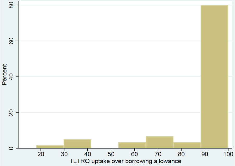
Figure 1: distribution of TLTRO uptake over borrowing allowance (%) for
banks participating in the
initial TLTROs
ECB Working Paper Series No 2364 / January 2020
64
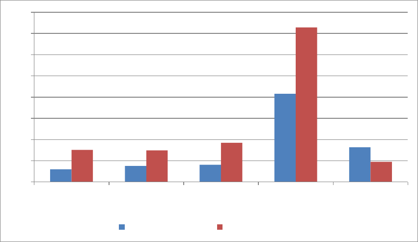
Figure 2: proportion of banks that eased credit standards/margins for
high and low values of
country TLTRO (loans to NFCs)
The figure displays the mean of the d
ependent variables (loans to NFCs) for two groups. A bank
belongs to the group “high country TLTRO” if the value of the variable country TLTRO
(
)
is higher
than the median (0.75); otherwise it belongs to the group “low country TLTRO”.
0.00
0.05
0.10
0.15
0.20
0.25
0.30
0.35
0.40
credit standards
overall
credit standards
sme
credit standards
large
average margins riskier margins
low country TLTRO high country TLTRO
ECB Working Paper Series No 2364 / January 2020
65
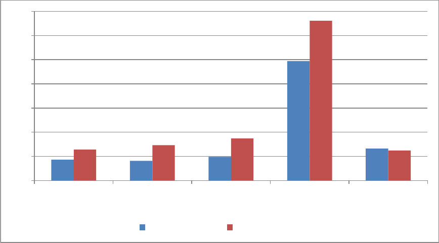
Figure 3: proportion of banks that eased credit standards/margins for high and low values of bank
TLTR
O (loans to NFCs)
The figure displays the mean of the d
ependent variables (loans to NFCs) for two groups. A bank
belongs to the group “high bank TLTRO” if the value of the variable bank TLTRO
is higher than the
median (0); otherwise it belongs to the group “low bank TLTRO”.
0.00
0.05
0.10
0.15
0.20
0.25
0.30
0.35
credit standards
overall
credit standards
sme
credit standards
large
average margins riskier margins
low bank TLTRO high bank TLTRO
ECB Working Paper Series No 2364 / January 2020
66

Acknowledgements
The views expressed in this paper are those of the authors and do not necessarily coincide with those of the European Central Bank,
Banco de España or the Eurosystem. We would like to thank Roberto Blanco, Clodomiro Ferreira, Ángel Gavilán, Ricardo Gimeno,
Sergio Mayordomo, Dominique Thaler, Juan Luis Vega, Ernesto Villanueva, seminar participants at Banco de España and an
anonymous referee for their useful comments and suggestions.
D
esislava C. Andreeva
European Central Bank, Frankfurt am Main, Germany; email: desislava.andreev[email protected]
M
iguel García-Posada (corresponding author)
Banco de España, Madrid, Spain; email: miguel.garcia-[email protected]
© European Central Bank, 2020
Postal address 60640 Frankfurt am Main, Germany
Telephone +49 69 1344 0
Website www.ecb.europa.eu
All rights reserved. Any reproduction, publication and reprint in the form of a different publication, whether printed or produced
electronically, in whole or in part, is permitted only with the explicit written authorisation of the ECB or the authors.
This paper can be downloaded without charge from www.ecb.europa.eu, from the Social Science Research Network electronic library or
from RePEc: Research Papers in Economics. Information on all of the papers published in the ECB Working Paper Series can be found
on the ECB’s website.
PDF ISBN 978-92-899-4007-8 ISSN 1725-2806 doi:10.2866/3836
QB-AR-20-016-EN-N
