
limma:
Linear Models for Microarray and RNA-Seq Data
User’s Guide
Gordon K. Smyth, Matthew Ritchie, Natalie Thorne,
James Wettenhall, Wei Shi and Yifang Hu
Bioinformatics Division, The Walter and Eliza Hall Institute
of Medical Research, Melbourne, Australia
First edition 2 December 2002
Last revised 22 April 2023
This free open-source software implements academic research
by the authors and co-workers. If you use it, please support
the project by citing the appropriate journal articles listed in
Section 2.1.
Contents
1 Introduction 5
2 Preliminaries 7
2.1 Citing limma . . . . . . . . . . . . . . . . . . . . . . . . . . . . . . . . . . . . . . . . . 7
2.2 Installation . . . . . . . . . . . . . . . . . . . . . . . . . . . . . . . . . . . . . . . . . . 9
2.3 How to get help . . . . . . . . . . . . . . . . . . . . . . . . . . . . . . . . . . . . . . . . 9
3 Quick Start 11
3.1 A brief introduction to R . . . . . . . . . . . . . . . . . . . . . . . . . . . . . . . . . . 11
3.2 Sample limma Session . . . . . . . . . . . . . . . . . . . . . . . . . . . . . . . . . . . . 12
3.3 Data Objects . . . . . . . . . . . . . . . . . . . . . . . . . . . . . . . . . . . . . . . . . 13
4 Reading Microarray Data 15
4.1 Scope of this Chapter . . . . . . . . . . . . . . . . . . . . . . . . . . . . . . . . . . . . 15
4.2 Recommended Files . . . . . . . . . . . . . . . . . . . . . . . . . . . . . . . . . . . . . 15
4.3 The Targets Frame . . . . . . . . . . . . . . . . . . . . . . . . . . . . . . . . . . . . . . 15
4.4 Reading Two-Color Intensity Data . . . . . . . . . . . . . . . . . . . . . . . . . . . . . 17
4.5 Reading Single-Channel Agilent Intensity Data . . . . . . . . . . . . . . . . . . . . . . 19
4.6 Reading Illumina BeadChip Data . . . . . . . . . . . . . . . . . . . . . . . . . . . . . . 19
4.7 Image-derived Spot Quality Weights . . . . . . . . . . . . . . . . . . . . . . . . . . . . 20
4.8 Reading Probe Annotation . . . . . . . . . . . . . . . . . . . . . . . . . . . . . . . . . 21
4.9 Printer Layout . . . . . . . . . . . . . . . . . . . . . . . . . . . . . . . . . . . . . . . . 22
4.10 The Spot Types File . . . . . . . . . . . . . . . . . . . . . . . . . . . . . . . . . . . . . 22
5 Quality Assessment 24
6 Pre-Processing Two-Color Data 26
6.1 Background Correction . . . . . . . . . . . . . . . . . . . . . . . . . . . . . . . . . . . . 26
6.2 Within-Array Normalization . . . . . . . . . . . . . . . . . . . . . . . . . . . . . . . . . 28
6.3 Between-Array Normalization . . . . . . . . . . . . . . . . . . . . . . . . . . . . . . . . 30
6.4 Using Objects from the marray Package . . . . . . . . . . . . . . . . . . . . . . . . . . 32
7 Filtering unexpressed probes 34
1
8 Linear Models Overview 36
8.1 Introduction . . . . . . . . . . . . . . . . . . . . . . . . . . . . . . . . . . . . . . . . . . 36
8.2 Single-Channel Designs . . . . . . . . . . . . . . . . . . . . . . . . . . . . . . . . . . . 37
8.3 Common Reference Designs . . . . . . . . . . . . . . . . . . . . . . . . . . . . . . . . . 38
8.4 Direct Two-Color Designs . . . . . . . . . . . . . . . . . . . . . . . . . . . . . . . . . . 39
9 Single-Channel Experimental Designs 41
9.1 Introduction . . . . . . . . . . . . . . . . . . . . . . . . . . . . . . . . . . . . . . . . . . 41
9.2 Two Groups . . . . . . . . . . . . . . . . . . . . . . . . . . . . . . . . . . . . . . . . . . 41
9.3 Several Groups . . . . . . . . . . . . . . . . . . . . . . . . . . . . . . . . . . . . . . . . 43
9.4 Additive Models and Blocking . . . . . . . . . . . . . . . . . . . . . . . . . . . . . . . . 43
9.4.1 Paired Samples . . . . . . . . . . . . . . . . . . . . . . . . . . . . . . . . . . . . 43
9.4.2 Blocking . . . . . . . . . . . . . . . . . . . . . . . . . . . . . . . . . . . . . . . . 44
9.5 Interaction Models: 2 × 2 Factorial Designs . . . . . . . . . . . . . . . . . . . . . . . . 44
9.5.1 Questions of Interest . . . . . . . . . . . . . . . . . . . . . . . . . . . . . . . . . 44
9.5.2 Analysing as for a Single Factor . . . . . . . . . . . . . . . . . . . . . . . . . . 45
9.5.3 A Nested Interaction Formula . . . . . . . . . . . . . . . . . . . . . . . . . . . . 46
9.5.4 Classic Interaction Models . . . . . . . . . . . . . . . . . . . . . . . . . . . . . . 46
9.6 Time Course Experiments . . . . . . . . . . . . . . . . . . . . . . . . . . . . . . . . . . 48
9.6.1 Replicated time points . . . . . . . . . . . . . . . . . . . . . . . . . . . . . . . . 48
9.6.2 Many time points . . . . . . . . . . . . . . . . . . . . . . . . . . . . . . . . . . . 49
9.7 Multi-level Experiments . . . . . . . . . . . . . . . . . . . . . . . . . . . . . . . . . . . 50
10 Two-Color Experiments with a Common Reference 52
10.1 Introduction . . . . . . . . . . . . . . . . . . . . . . . . . . . . . . . . . . . . . . . . . . 52
10.2 Two Groups . . . . . . . . . . . . . . . . . . . . . . . . . . . . . . . . . . . . . . . . . . 52
10.3 Several Groups . . . . . . . . . . . . . . . . . . . . . . . . . . . . . . . . . . . . . . . . 54
11 Direct Two-Color Experimental Designs 55
11.1 Introduction . . . . . . . . . . . . . . . . . . . . . . . . . . . . . . . . . . . . . . . . . . 55
11.2 Simple Comparisons . . . . . . . . . . . . . . . . . . . . . . . . . . . . . . . . . . . . . 55
11.2.1 Replicate Arrays . . . . . . . . . . . . . . . . . . . . . . . . . . . . . . . . . . . 55
11.2.2 Dye Swaps . . . . . . . . . . . . . . . . . . . . . . . . . . . . . . . . . . . . . . 56
11.3 A Correlation Approach to Technical Replication . . . . . . . . . . . . . . . . . . . . . 57
12 Separate Channel Analysis of Two-Color Data 59
13 Statistics for Differential Expression 61
13.1 Summary Top-Tables . . . . . . . . . . . . . . . . . . . . . . . . . . . . . . . . . . . . . 61
13.2 Fitted Model Objects . . . . . . . . . . . . . . . . . . . . . . . . . . . . . . . . . . . . 62
13.3 Multiple Testing Across Contrasts . . . . . . . . . . . . . . . . . . . . . . . . . . . . . 63
14 Array Quality Weights 65
14.1 Introduction . . . . . . . . . . . . . . . . . . . . . . . . . . . . . . . . . . . . . . . . . . 65
14.2 Example 1 . . . . . . . . . . . . . . . . . . . . . . . . . . . . . . . . . . . . . . . . . . . 65
14.3 Example 2 . . . . . . . . . . . . . . . . . . . . . . . . . . . . . . . . . . . . . . . . . . . 67
14.4 When to Use Array Weights . . . . . . . . . . . . . . . . . . . . . . . . . . . . . . . . . 69
2
15 RNA-Seq Data 70
15.1 Introduction . . . . . . . . . . . . . . . . . . . . . . . . . . . . . . . . . . . . . . . . . . 70
15.2 Making a count matrix . . . . . . . . . . . . . . . . . . . . . . . . . . . . . . . . . . . . 70
15.3 Normalization and filtering . . . . . . . . . . . . . . . . . . . . . . . . . . . . . . . . . 70
15.4 Differential expression: limma-trend . . . . . . . . . . . . . . . . . . . . . . . . . . . . 71
15.5 Differential expression: voom . . . . . . . . . . . . . . . . . . . . . . . . . . . . . . . . 71
15.6 Voom with sample quality weights . . . . . . . . . . . . . . . . . . . . . . . . . . . . . 72
15.7 Differential splicing . . . . . . . . . . . . . . . . . . . . . . . . . . . . . . . . . . . . . . 74
16 Two-Color Case Studies 76
16.1 Swirl Zebrafish: A Single-Group Experiment . . . . . . . . . . . . . . . . . . . . . . . 76
16.2 Apoa1 Knockout Mice: A Two-Group Common-Reference Experiment . . . . . . . . . 87
16.3 Weaver Mutant Mice: A Composite 2x2 Factorial Experiment . . . . . . . . . . . . . . 90
16.3.1 Background . . . . . . . . . . . . . . . . . . . . . . . . . . . . . . . . . . . . . . 90
16.3.2 Sample Preparation and Hybridizations . . . . . . . . . . . . . . . . . . . . . . 90
16.3.3 Data input . . . . . . . . . . . . . . . . . . . . . . . . . . . . . . . . . . . . . . 91
16.3.4 Annotation . . . . . . . . . . . . . . . . . . . . . . . . . . . . . . . . . . . . . . 92
16.3.5 Quality Assessment and Normalization . . . . . . . . . . . . . . . . . . . . . . . 92
16.3.6 Setting Up the Linear Model . . . . . . . . . . . . . . . . . . . . . . . . . . . . 94
16.3.7 Probe Filtering and Array Quality Weights . . . . . . . . . . . . . . . . . . . . 95
16.3.8 Differential expression . . . . . . . . . . . . . . . . . . . . . . . . . . . . . . . . 95
16.4 Bob1 Mutant Mice: Arrays With Duplicate Spots . . . . . . . . . . . . . . . . . . . . . 96
17 Single-Channel Case Studies 100
17.1 Lrp Mutant E. Coli Strain with Affymetrix Arrays . . . . . . . . . . . . . . . . . . . . 100
17.1.1 Background . . . . . . . . . . . . . . . . . . . . . . . . . . . . . . . . . . . . . . 100
17.1.2 Downloading the data . . . . . . . . . . . . . . . . . . . . . . . . . . . . . . . . 100
17.1.3 Background correction and normalization . . . . . . . . . . . . . . . . . . . . . 101
17.1.4 Gene annotation . . . . . . . . . . . . . . . . . . . . . . . . . . . . . . . . . . . 101
17.1.5 Differential expression . . . . . . . . . . . . . . . . . . . . . . . . . . . . . . . . 102
17.2 Effect of Estrogen on Breast Cancer Tumor Cells: A 2x2 Factorial Experiment with
Affymetrix Arrays . . . . . . . . . . . . . . . . . . . . . . . . . . . . . . . . . . . . . . 104
17.3 Comparing Mammary Progenitor Cell Populations with Illumina BeadChips . . . . . . 108
17.3.1 Introduction . . . . . . . . . . . . . . . . . . . . . . . . . . . . . . . . . . . . . 108
17.3.2 The target RNA samples . . . . . . . . . . . . . . . . . . . . . . . . . . . . . . 109
17.3.3 The expression profiles . . . . . . . . . . . . . . . . . . . . . . . . . . . . . . . . 110
17.3.4 How many probes are truly expressed? . . . . . . . . . . . . . . . . . . . . . . . 111
17.3.5 Normalization and filtering . . . . . . . . . . . . . . . . . . . . . . . . . . . . . 111
17.3.6 Within-patient correlations . . . . . . . . . . . . . . . . . . . . . . . . . . . . . 112
17.3.7 Differential expression between cell types . . . . . . . . . . . . . . . . . . . . . 112
17.3.8 Signature genes for luminal progenitor cells . . . . . . . . . . . . . . . . . . . . 113
17.4 Time Course Effects of Corn Oil on Rat Thymus with Agilent 4x44K Arrays . . . . . 114
17.4.1 Introduction . . . . . . . . . . . . . . . . . . . . . . . . . . . . . . . . . . . . . 114
17.4.2 Data availability . . . . . . . . . . . . . . . . . . . . . . . . . . . . . . . . . . . 114
17.4.3 Reading the data . . . . . . . . . . . . . . . . . . . . . . . . . . . . . . . . . . . 115
17.4.4 Gene annotation . . . . . . . . . . . . . . . . . . . . . . . . . . . . . . . . . . . 116
3
17.4.5 Background correction and normalize . . . . . . . . . . . . . . . . . . . . . . . 116
17.4.6 Gene filtering . . . . . . . . . . . . . . . . . . . . . . . . . . . . . . . . . . . . . 117
17.4.7 Differential expression . . . . . . . . . . . . . . . . . . . . . . . . . . . . . . . . 117
17.4.8 Gene ontology analysis . . . . . . . . . . . . . . . . . . . . . . . . . . . . . . . . 118
18 RNA-Seq Case Studies 120
18.1 Profiles of Yoruba HapMap Individuals . . . . . . . . . . . . . . . . . . . . . . . . . . . 120
18.1.1 Background . . . . . . . . . . . . . . . . . . . . . . . . . . . . . . . . . . . . . . 120
18.1.2 Data availability . . . . . . . . . . . . . . . . . . . . . . . . . . . . . . . . . . . 120
18.1.3 Yoruba Individuals and FASTQ Files . . . . . . . . . . . . . . . . . . . . . . . 120
18.1.4 Mapping reads to the reference genome . . . . . . . . . . . . . . . . . . . . . . 122
18.1.5 Annotation . . . . . . . . . . . . . . . . . . . . . . . . . . . . . . . . . . . . . . 124
18.1.6 DGEList object . . . . . . . . . . . . . . . . . . . . . . . . . . . . . . . . . . . . 125
18.1.7 Filtering . . . . . . . . . . . . . . . . . . . . . . . . . . . . . . . . . . . . . . . . 125
18.1.8 Scale normalization . . . . . . . . . . . . . . . . . . . . . . . . . . . . . . . . . 125
18.1.9 Linear modeling . . . . . . . . . . . . . . . . . . . . . . . . . . . . . . . . . . . 127
18.1.10 Gene set testing . . . . . . . . . . . . . . . . . . . . . . . . . . . . . . . . . . . 130
18.1.11 Session information . . . . . . . . . . . . . . . . . . . . . . . . . . . . . . . . . . 133
18.1.12 Acknowledgements . . . . . . . . . . . . . . . . . . . . . . . . . . . . . . . . . . 134
18.2 Differential Splicing after Pasilla Knockdown . . . . . . . . . . . . . . . . . . . . . . . 134
18.2.1 Background . . . . . . . . . . . . . . . . . . . . . . . . . . . . . . . . . . . . . . 134
18.2.2 GEO samples and SRA Files . . . . . . . . . . . . . . . . . . . . . . . . . . . . 134
18.2.3 Mapping reads to the reference genome . . . . . . . . . . . . . . . . . . . . . . 135
18.2.4 Read counts for exons . . . . . . . . . . . . . . . . . . . . . . . . . . . . . . . . 136
18.2.5 Assemble DGEList and sum counts for technical replicates . . . . . . . . . . . 136
18.2.6 Gene annotation . . . . . . . . . . . . . . . . . . . . . . . . . . . . . . . . . . . 137
18.2.7 Filtering . . . . . . . . . . . . . . . . . . . . . . . . . . . . . . . . . . . . . . . . 138
18.2.8 Scale normalization . . . . . . . . . . . . . . . . . . . . . . . . . . . . . . . . . 138
18.2.9 Linear modelling . . . . . . . . . . . . . . . . . . . . . . . . . . . . . . . . . . . 139
18.2.10 Alternate splicing . . . . . . . . . . . . . . . . . . . . . . . . . . . . . . . . . . . 141
18.2.11 Session information . . . . . . . . . . . . . . . . . . . . . . . . . . . . . . . . . . 144
18.2.12 Acknowledgements . . . . . . . . . . . . . . . . . . . . . . . . . . . . . . . . . . 145
4
Chapter 1
Introduction
Limma is a package for the analysis of gene expression data arising from microarray or RNA-seq
technologies [27]. A core capability is the use of linear models to assess differential expression in
the context of multi-factor designed experiments. Limma provides the ability to analyze comparisons
between many RNA targets simultaneously. It has features that make the analyses stable even for
experiments with small number of arrays—this is achieved by borrowing information across genes.
It is specially designed for analysing complex experiments with a variety of experimental conditions
and predictors. The linear model and differential expression functions are applicable to data from
any quantitative gene expression technology including microarrays, RNA-seq and quantitative PCR.
Limma can handle both single-channel and two-color microarrays.
This guide gives a tutorial-style introduction to the main limma features but does not describe
every feature of the package. A full description of the package is given by the individual func-
tion help documents available from the R online help system. To access the online help, type
help(package=limma) at the R prompt or else start the html help system using help.start() or the
Windows drop-down help menu.
Limma provides a strong suite of functions for reading, exploring and pre-processing data from
two-color microarrays. The Bioconductor package marray provides alternative functions for reading
and normalizing spotted two-color microarray data. The marray package provides flexible location
and scale normalization routines for log-ratios from two-color arrays. The limma package overlaps
with marray in functionality but is based on a more general concept of within-array and between-array
normalization as separate steps. If you are using limma in conjunction with marray, see Section 6.4.
Limma can read output data from a variety of image analysis software platforms, including
GenePix, ImaGene etc. Either one-channel or two-channel formats can be processed.
The Bioconductor package affy provides functions for reading and normalizing Affymetrix mi-
croarray data. Advice on how to use limma with the affy package is given throughout the User’s
Guide, see for example Section 8.2 and the E. coli and estrogen case studies.
Functions for reading and pre-processing expression data from Illumina BeadChips were intro-
duced in limma 3.0.0. See the case study in Section 17.3 for an example of these. Limma can also be
used in conjunction with the vst or beadarray packages for pre-processing Illumina data.
From version 3.9.19, limma includes functions to analyse RNA-seq experiments, demonstrated
in Case Study 11.8. The approach is to convert a table of sequence read counts into an expression
object which can then be analysed as for microarray data.
This guide describes limma as a command-driven package. Graphical user interfaces to the most
commonly used functions in limma are available through the packages limmaGUI [39], for two-color
5
data, or affylmGUI [38], for Affymetrix data. Both packages are available from Bioconductor.
This user’s guide should be correct for R Versions 2.8.0 through 4.0.0 and limma versions 2.16.0
through 3.44.0. The limma homepage is https://bioinf.wehi.edu.au/limma.
6
Chapter 2
Preliminaries
2.1 Citing limma
Limma implements a body of methodological research by the authors and co-workers. Please try to
cite the appropriate papers when you use results from the limma software in a publication, as such
citations are the main means by which the authors receive professional credit for their work.
The limma software package itself can be cited as:
Ritchie, ME, Phipson, B, Wu, D, Hu, Y, Law, CW, Shi, W, and Smyth, GK (2015).
limma powers differential expression analyses for RNA-sequencing and microarray studies.
Nucleic Acids Research 43(7), e47.
The above article reviews the overall capabilities of the limma package, both new and old.
Other articles describe the statistical methodology behind particular functions of the package. If
you use limma for differential expression analysis, please cite:
Phipson, B, Lee, S, Majewski, IJ, Alexander, WS, and Smyth, GK (2016). Robust
hyperparameter estimation protects against hypervariable genes and improves power to
detect differential expression. Annals of Applied Statistics 10(2), 946–963.
This article describes the linear modeling approach implemented by lmFit and the empirical Bayes
statistics implemented by eBayes, topTable etc. It particularly describes eBayes with robust=TRUE or
trend=TRUE.
If you use limma for RNA-seq analysis, please cite either:
Law, CW, Chen, Y, Shi, W, and Smyth, GK (2014). Voom: precision weights unlock
linear model analysis tools for RNA-seq read counts. Genome Biology 15, R29.
or
Liu, R, Holik, AZ, Su, S, Jansz, N, Chen, K, Leong, HS, Blewitt, ME, Asselin-Labat,
M-L, Smyth, GK, Ritchie, ME (2015). Why weight? Modelling sample and observational
level variability improves power in RNA-seq analyses. Nucleic Acids Research 43, e97.
Law et al (2014) describe the voom and limma-trend pipelines for RNA-seq, while Liu et al (2015)
describe the voomWithQualityWeights function.
If you use limma with duplicate spots or technical replication, please cite
7
Smyth, G. K., Michaud, J., and Scott, H. (2005). The use of within-array replicate spots
for assessing differential expression in microarray experiments. Bioinformatics 21, 2067–
2075.
http://www.statsci.org/smyth/pubs/dupcor.pdf
The above article describes the theory behind the duplicateCorrelation function.
If you use limma for normalization of two-color microarray data, please cite one of:
Smyth, G. K., and Speed, T. P. (2003). Normalization of cDNA microarray data. Methods
31, 265–273.
http://www.statsci.org/smyth/pubs/normalize.pdf
Oshlack, A., Emslie, D., Corcoran, L., and Smyth, G. K. (2007). Normalization of
boutique two-color microarrays with a high proportion of differentially expressed probes.
Genome Biology 8, R2.
The first of these articles describes the functions read.maimages, normalizeWithinArrays and normalize-
BetweenArrays. The second describes the use of spot quality weights to normalize on control probes.
The various options provided by the backgroundCorrect function are explained by:
Ritchie, M. E., Silver, J., Oshlack, A., Silver, J., Holmes, M., Diyagama, D., Holloway, A.,
and Smyth, G. K. (2007). A comparison of background correction methods for two-colour
microarrays. Bioinformatics 23, 2700–2707.
If you use arrayWeights or related functions to estimate sample quality weights, please cite:
Ritchie, M. E., Diyagama, D., Neilson, van Laar, R., J., Dobrovic, A., Holloway, A., and
Smyth, G. K. (2006). Empirical array quality weights in the analysis of microarray data.
BMC Bioinformatics 7, 261.
If you use the read.ilmn, nec or neqc functions to process Illumina BeadChip data, please cite:
Shi, W, Oshlack, A, and Smyth, GK (2010). Optimizing the noise versus bias trade-off
for Illumina Whole Genome Expression BeadChips. Nucleic Acids Research 38, e204.
The propexpr function is explained by
Shi, W, de Graaf, C, Kinkel, S, Achtman, A, Baldwin, T, Schofield, L, Scott, H, Hilton,
D, Smyth, GK (2010). Estimating the proportion of microarray probes expressed in an
RNA sample. Nucleic Acids Research 38, 2168–2176.
The lmscFit function for separate channel analysis of two-color microarray data is explained by:
Smyth, GK, and Altman, NS (2013). Separate-channel analysis of two-channel microar-
rays: recovering inter-spot information. BMC Bioinformatics 14, 165.
Finally, if you are using one of the menu-driven interfaces to the software, please cite the appro-
priate one of
Wettenhall, J. M., and Smyth, G. K. (2004). limmaGUI: a graphical user interface for
linear modeling of microarray data. Bioinformatics, 20, 3705–3706.
Wettenhall, J. M., Simpson, K. M., Satterley, K., and Smyth, G. K. (2006). affylmGUI:
a graphical user interface for linear modeling of single channel microarray data. Bioin-
formatics 22, 897–899.
8
2.2 Installation
Limma is a package for the R computing environment and we will assume here that you have already
installed R (if not, see the R project at http://www.r-project.org). To install the latest version
of limma, you will need to be using the latest version of R.
Limma is part of the Bioconductor project at http://www.bioconductor.org. Like other Bio-
conductor packages, limma is most easily installed using the BiocManager package:
> library(BiocManager)
> install("limma")
This will allow you do to perform many basic analyses, although you’ll probably want
> install("statmod")
as well. If you’re starting from scratch and haven’t used any Bioconductor packages before, then
you will need to install the BiocManager package itself by install.packages("BiocManager" before
installing limma.
Bioconductor works on a 6-monthly official release cycle, lagging each major R release by a short
time. As with other Bioconductor packages, there are always two versions of limma. Most users will
use the current official release version, which will be installed by BiocManager::install if you are
using the current version of R. There is also a developmental version of limma that includes new
features due for the next official release. The developmental version will be installed if you are using
the developmental version of R. The official release version always has an even second number (for
example 3.6.5), whereas the developmental version has an odd second number (for example 3.7.7).
Limma is updated frequently. To see what new features were introduced in the latest Bioconductor
release, type:
> news(package = "limma")
There is also a detailed change-log that describes each minor update. To see the most recent 20 lines
of the change-log type:
> changeLog(n = 20)
2.3 How to get help
Most questions about limma will hopefully be answered by the documentation or references. If you’ve
run into a question which isn’t addressed by the documentation, or you’ve found a conflict between
the documentation and software itself, then there is an active support community that can offer help.
The authors of the package always appreciate receiving reports of bugs in the package functions
or in the documentation. The same goes for well-considered suggestions for improvements. All
other questions or problems concerning limma should be posted to the Bioconductor support site
https://support.bioconductor.org. Please send requests for general assistance and advice to the
support site rather than to the individual authors. Posting questions to the Bioconductor mailing
list has a number of advantages. First, the mailing list includes a community of experienced limma
users who can answer most common questions. Second, the limma authors try hard to ensure that
any user posting to Bioconductor receives assistance. Third, the mailing list allows others with the
same sort of questions to gain from the answers. Users posting to the mailing list for the first time
9
will find it helpful to read the posting guide at http://www.bioconductor.org/help/support/
posting-guide.
Note that each function in limma has its own online help page, as described in the next chapter.
If you have a question about any particular function, reading the function’s help page will often
answer the question very quickly. In any case, it is good etiquette to check the relevant help page
first before posting a question to the support site.
10
Chapter 3
Quick Start
3.1 A brief introduction to R
R is a program for statistical computing. It is a command-driven language meaning that you have
to type commands into it rather than pointing and clicking using a mouse. In this guide it will be
assumed that you have successfully downloaded and installed R from http://www.r-project.org.
A good way to get started is to type
> help.start()
at the R prompt or, if you’re using R for Windows, to follow the drop-down menu items Help Html
help. Following the links Packages limma from the html help page will lead you to the contents
page of help topics for functions in limma.
Before you can use any limma commands you have to load the package by typing
> library(limma)
at the R prompt. You can get help on any function in any loaded package by typing ? and the
function name at the R prompt, for example
> ?lmFit
or equivalently
> help("lmFit")
for detailed help on the lmFit function. The individual function help pages are especially important
for listing all the arguments which a function will accept and what values the arguments can take.
A key to understanding R is to appreciate that anything that you create in R is an “object”.
Objects might include data sets, variables, functions, anything at all. For example
> x <- 2
will create a variable x and will assign it the value 2. At any stage of your R session you can type
> objects()
to get a list of all the objects you have created. You can see the contents of any object by typing
the name of the object at the prompt, for example either of the following commands will print out
the contents of x:
11
> show(x)
> x
We hope that you can use limma without having to spend a lot of time learning about the R
language itself but a little knowledge in this direction will be very helpful, especially when you want
to do something not explicitly provided for in limma or in the other Bioconductor packages. For
more details about the R language see An Introduction to R which is available from the online help.
For more background on using R for statistical analyses see [6].
3.2 Sample limma Session
This is a quick overview of what an analysis might look like. The first example assumes four replicate
two-color arrays, the second and fourth of which are dye-swapped. We assume that the images have
been analyzed using GenePix to produce a .gpr file for each array and that a targets file targets.txt
has been prepared with a column containing the names of the .gpr files.
> library(limma)
> targets <- readTargets("targets.txt")
Set up a filter so that any spot with a flag of −99 or less gets zero weight.
> f <- function(x) as.numeric(x$Flags > -99)
Read in the data.
> RG <- read.maimages(targets, source="genepix", wt.fun=f)
The following command implements a type of adaptive background correction. This is optional but
recommended for GenePix data.
> RG <- backgroundCorrect(RG, method="normexp", offset=50)
Print-tip loess normalization:
> MA <- normalizeWithinArrays(RG)
Estimate the fold changes and standard errors by fitting a linear model for each gene. The design
matrix indicates which arrays are dye-swaps.
> fit <- lmFit(MA, design=c(-1,1,-1,1))
Apply empirical Bayes smoothing to the standard errors.
> fit <- eBayes(fit)
Show statistics for the top 10 genes.
> topTable(fit)
The second example assumes Affymetrix arrays hybridized with either wild-type (wt) or mutant
(mu) RNA. There should be three or more arrays in total to ensure some replication. The targets
file is now assumed to have another column Genotype indicating which RNA source was hybridized
on each array.
12
> library(gcrma)
> library(limma)
> targets <- readTargets("targets.txt")
Read and pre-process the Affymetrix CEL file data.
> ab <- ReadAffy(filenames=targets$FileName)
> eset <- gcrma(ab)
Form an appropriate design matrix for the two RNA sources and fit linear models. The design matrix
has two columns. The first represents log-expression in the wild-type and the second represents the
log-ratio between the mutant and wild-type samples. See Section 9.2 for more details on the design
matrix.
> design <- cbind(WT=1, MUvsWT=targets$Genotype=="mu")
> fit <- lmFit(eset, design)
> fit <- eBayes(fit)
> topTable(fit, coef="MUvsWT")
This code fits the linear model, smooths the standard errors and displays the top 10 genes for the
mutant versus wild-type comparison.
The options trend=TRUE and robust=TRUE are also often helpful when running eBayes, increasing
power for certain types of data. For example:
> fit <- eBayes(fit, trend=TRUE, robust=TRUE)
> topTable(fit, coef="MUvsWT")
3.3 Data Objects
There are six main types of data objects created and used in limma:
EListRaw. Raw Expression list. A class used to store single-channel raw intensities prior to
normalization. Intensities are unlogged. Objects of this class contain one row for each probe
and one column for each array. The function read.ilmn() for example creates an object of this
class.
EList. Expression list. Contains background corrected and normalized log-intensities. Usually
created from an EListRaw objecting using normalizeBetweenArrays() or neqc().
RGList. Red-Green list. A class used to store raw two-color intensities as they are read in from an
image analysis output file, usually by read.maimages().
MAList. Two-color intensities converted to M-values and A-values, i.e., to within-spot and whole-
spot contrasts on the log-scale. Usually created from an RGList using MA.RG() or normalizeWithinArrays().
Objects of this class contain one row for each spot. There may be more than one spot and
therefore more than one row for each probe.
MArrayLM. MicroArray Linear Model. Store the result of fitting gene-wise linear models to the
normalized intensities or log-ratios. Usually created by lmFit(). Objects of this class normally
contain one row for each unique probe.
13
TestResults. Store the results of testing a set of contrasts equal to zero for each probe. Usually
created by decideTests(). Objects of this class normally contain one row for each unique
probe.
All these objects can be treated like any list in R. For example, MA M extracts the matrix of M-values
if MA is an MAList object, or fit coef extracts the coefficient estimates if fit is an MArrayLM object.
names(MA) shows what components are contained in the object. For those who are familiar with
matrices in R, all these objects are also designed to obey many analogies with matrices. In the case
of RGList and MAList, rows correspond to spots and columns to arrays. In the case of MarrayLM, rows
correspond to unique probes and columns to parameters or contrasts. The functions summary, dim,
length, ncol, nrow, dimnames, rownames, colnames have methods for these classes. For example
> dim(RG)
[1] 11088 4
shows that the RGList object RG contains data for 11088 spots and 4 arrays.
> colnames(RG)
will give the names of the filenames or arrays in the object, while if fit is an MArrayLM object then
> colnames(fit)
would give the names of the coefficients in the linear model fit.
Objects of any of these classes may be subsetted, so that RG[,j] means the data for array j and
RG[i,] means the data for probes indicated by the index i. Multiple data objects may be combined
using cbind, rbind or merge. Hence
> RG1 <- read.maimages(files[1:2], source="genepix")
> RG2 <- read.maimages(files[3:5], source="genepix")
> RG <- cbind(RG1, RG2)
is equivalent to
> RG <- read.maimages(files[1:5], source="genepix")
Alternatively, if control status has been set in the MAList object then
> i <- MA$genes$Status=="Gene"
> MA[i,]
might be used to eliminate control spots from the data object prior to fitting a linear model.
14
Chapter 4
Reading Microarray Data
4.1 Scope of this Chapter
This chapter covers most microarray types other than Affymetrix. To read data from Affymetrix
GeneChips, please use the affy, gcrma or aroma.affymetrix packages to read and normalize the data.
4.2 Recommended Files
We assume that an experiment has been conducted with one or more microarrays, all printed with
the same library of probes. Each array has been scanned to produce a TIFF image. The TIFF
images have then been processed using an image analysis program such a ArrayVision, ImaGene,
GenePix, QuantArray or SPOT to acquire the red and green foreground and background intensities
for each spot. The spot intensities have then been exported from the image analysis program into
a series of text files. There should be one file for each array or, in the case of Imagene, two files for
each array.
You will need to have the image analysis output files. In most cases these files will include the IDs
and names of the probes and possibly other annotation information. A few image analysis programs,
for example SPOT, do not write the probe IDs into the output files. In this case you will also need a
genelist file which describes the probes. It most cases it is also desirable to have a targets file which
describes which RNA sample was hybridized to each channel of each array. A further optional file is
the spot types file which identifies special probes such as control spots.
4.3 The Targets Frame
The first step in preparing data for input into limma is usually to create a targets file which lists the
RNA target hybridized to each channel of each array. It is normally in tab-delimited text format
and should contain a row for each microarray in the experiment. The file can have any name but
the default is Targets.txt. If it has the default name, it can be read into the R session using
> targets <- readTargets()
Once read into R, it becomes the targets frame.
The targets frame normally contains a FileName column, giving the name of the image-analysis
output file, a Cy3 column giving the RNA type labeled with Cy3 dye for that slide and a Cy5
15
column giving the RNA type labeled with Cy5 dye for that slide. Other columns are optional. The
targets file can be prepared using any text editor but spreadsheet programs such as Microsoft Excel
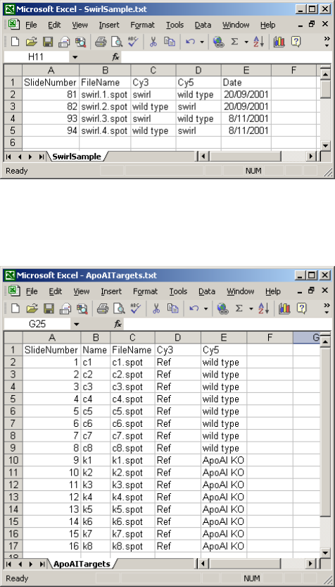
are convenient. The targets file for the Swirl case study includes optional SlideNumber and Date
columns:
It is often convenient to create short readable labels to associate with each array for use in output
and in plots, especially if the file names are long or non-intuitive. A column containing these labels
can be included in the targets file, for example the Name column used for the Apoa1 case study:
This column can be used to created row names for the targets frame by
> targets <- readTargets("targets.txt", row.names="Name")
The row names can be propagated to become array names in the data objects when these are read
in.
For ImaGene files, the FileName column is split into a FileNameCy3 column and a FileNameCy5
because ImaGene stores red and green intensities in separate files. This is a short example:
16
4.4 Reading Two-Color Intensity Data
Let files be a character vector containing the names of the image analysis output files. The fore-
ground and background intensities can be read into an RGList object using a command of the form
> RG <- read.maimages(files, source="<imageanalysisprogram>", path="<directory>")
where <imageanalysisprogram> is the name of the image analysis program and <directory> is the
full path of the directory containing the files. If the files are in the current R working directory then
the argument path can be omitted; see the help entry for setwd for how to set the current working
directory. The file names are usually read from the Targets File. For example, the Targets File
Targets.txt is in the current working directory together with the SPOT output files, then one might
use
> targets <- readTargets()
> RG <- read.maimages(targets$FileName, source="spot")
Alternatively, and even more simply, one may give the targets frame itself in place of the files
argument as
> RG <- read.maimages(targets, source="spot")
In this case the software will look for the column FileName in the targets frame.
If the files are GenePix output files then they might be read using
> RG <- read.maimages(targets, source="genepix")
given an appropriate targets file. Consult the help entry for read.maimages to see which other image
analysis programs are supported. Files are assumed by default to be tab-delimited, although other
separators can be specified using the sep= argument.
Reading data from ImaGene software is a little different to that of other image analysis programs
because the red and green intensities are stored in separate files. This means that the targets frame
should include two filename columns called, say, FileNameCy3 and FileNameCy5, giving the names of
the files containing the green and red intensities respectively. An example is given in Section 4.3.
Typical code with ImaGene data might be
> targets <- readTargets()
> files <- targets[,c("FileNameCy3","FileNameCy5")]
> RG <- read.maimages(files, source="imagene")
For ImaGene data, the files argument to read.maimages() is expected to be a 2-column matrix of
filenames rather than a vector.
The following table gives the default estimates used for the foreground and background intensities:
17

Source Foreground Background
agilent Median Signal Median Signal
agilent.mean Mean Signal Median Signal
agilent.median Median Signal Median Signal
bluefuse AMPCH None
genepix F Mean B Median
genepix.median F Median B Median
genepix.custom Mean B
imagene Signal Mean Signal Median, or Signal Mean if auto
segmentation has been used
quantarray Intensity Background
scanarrayexpress Mean Median
smd.old I MEAN B MEDIAN
smd Intensity (Mean) Background (Median)
spot mean morph
spot.close.open mean morph.close.open
The default estimates can be over-ridden by specifying the columns argument to read.maimages().
Suppose for example that GenePix has been used with a custom background method, and you wish
to use median foreground estimates. This combination of foreground and background is not provided
as a pre-set choice in limma, but you can specify it by
> RG <- read.maimages(files,source="genepix",
+ columns=list(R="F635 Median",G="F532 Median",Rb="B635",Gb="B532"))
What should you do if your image analysis program is not in the above list? If the image output
files are in standard format, then you can supply the annotation and intensity column names yourself.
For example,
> RG <- read.maimages(files,
+ columns=list(R="F635 Mean",G="F532 Mean",Rb="B635 Median",Gb="B532 Median"),
+ annotation=c("Block","Row","Column","ID","Name"))
is exactly equivalent to source="genepix". “Standard format” means here that there is a unique
column name identifying each column of interest and that there are no lines in the file following the
last line of data. Header information at the start of the file is acceptable, but extra lines at the end
of the file will cause the read to fail.
It is a good idea to look at your data to check that it has been read in correctly. Type
> show(RG)
to see a print out of the first few lines of data. Also try
> summary(RG$R)
to see a five-number summary of the red intensities for each array, and so on.
It is possible to read the data in several steps. If RG1 and RG2 are two data sets corresponding to
different sets of arrays then
> RG <- cbind(RG1, RG2)
will combine them into one large data set. Data sets can also be subsetted. For example RG[,1] is
the data for the first array while RG[1:100,] is the data on the first 100 genes.
18

4.5 Reading Single-Channel Agilent Intensity Data
Reading single-channel data is similar to two-color data, except that the argument green.only=TRUE
should be added to tell read.maimages() not to expect a red channel. Single-channel Agilent inten-
sities, as produced by Agilent’s Feature Extraction software, can be read by
> x <- read.maimages(files, source="agilent", green.only=TRUE)
or
> x <- read.maimages(targets, source="agilent", green.only=TRUE)
As for two-color data, the path argument is used:
> x <- read.maimages(files, source="agilent", path="<directory>", green.only=TRUE)
if the data files are not in the current working directory. The green.only argument tells read.maimages()
to output an EList object instead an RGList. The raw intensities will be stored in the E component
of the data object, and can be checked for example by
> summary(x$E)
Agilent’s Feature Extraction software has the ability to estimate the foreground and background
signals for each spot using either the mean or the median of the foreground and background pixels.
The default for read.maimages is to read the median signal for both foreground and background.
Alternatively
> x <- read.maimages(targets, source="agilent.mean", green.only=TRUE)
would read the mean foreground signal while still using median for the background. The possible
values for source are:
Source Foreground Background
agilent Median Signal Median Signal
agilent.mean Mean Signal Median Signal
agilent.median Median Signal Median Signal
As for two-color data, the default choices for the foreground and background estimates can be over-
ridden by specifying the columns argument to read.maimages().
Agilent Feature Extraction output files contain probe annotation columns as well as intensity
columns. By default, read.maimages() will read the following annotation columns, if they exist:
Row, Col, Start, Sequence, SwissProt, GenBank, Primate, GenPept, ProbeUID, ControlType, ProbeName,
GeneName, SystematicName, Description.
See Section 17.4 for a complete worked case study with single-channel Agilent data.
4.6 Reading Illumina BeadChip Data
Illumina whole-genome BeadChips require special treatment. Illumina images are scanned by Bead-
Scan software, and Illumina’s BeadStudio or GenomeStudio software can be used to export probe
summary profiles. The probe summary profiles are tab-delimited files containing the intensity data.
Typically, all the arrays processed at one time are written to a single file, with several columns cor-
responding to each array. We recommend that intensities should be exported from GenomeStudio
19
without background correction or normalization, as these pre-processing steps can be better done by
limma functions. GenomeStudio can also be asked to export profiles for the control probes, and we
recommend that this be done as well.
Illumina files differ from other platforms in that each image output file contains data from multiple
arrays and in that intensities for control probes are written to a separate file from the regular probes.
There are other features of these files that can optionally be used for pre-processing and filtering.
Illumina probe summary files can be read by the read.ilmn function. A typical usage is
> x <- read.ilmn("probe profile.txt", ctrlfiles="control probe profile.txt")
where probe profile.txt is the name of the main probe summary profile file and control probe
profile.txt is the name of the file containing profiles for control probes.
If there are multiple probe summary profiles to be read, and the samples are summarized in a
targets frame, then the read.ilmn.targets function can be used.
Reading the control probe profiles is optional but recommended. If the control probe profiles are
available, then the Illumina data can be favorably background corrected and normalized using the
neqc or nec functions. Otherwise, Illumina data is background corrected and normalized as for other
single channel platforms.
See Section 17.3 for a fully worked case study with Illumina microarray data.
4.7 Image-derived Spot Quality Weights
Image analysis programs typically output a lot of information, in addition to the foreground and
background intensities, which provides information on the quality of each spot. It is sometimes
desirable to use this information to produce a quality index for each spot which can be used in
the subsequent analysis steps. One approach is to remove all spots from consideration which do
not satisfy a certain quality criterion. A more sophisticated approach is to produce a quantitative
quality index which can be used to up or downweight each spot in a graduated way depending on
its perceived reliability. limma provides an approach to spot weights which supports both of these
approaches.
The limma approach is to compute a quantitative quality weight for each spot. Weights are
treated similarly in limma as they are treated in most regression functions in R such as lm(). A
zero weight indicates that the spot should be ignored in all analysis as being unreliable. A weight
of 1 indicates normal quality. A spot quality weight greater or less than one will result in that spot
being given relatively more or less weight in subsequent analyses. Spot weights less than zero are
not meaningful.
The quality information can be read and the spot quality weights computed at the same time as
the intensities are read from the image analysis output files. The computation of the quality weights
is defined by the wt.fun argument to the read.maimages() function. This argument is a function
which defines how the weights should be computed from the information found in the image analysis
files. Deriving good spot quality weights is far from straightforward and depends very much on the
image analysis software used. limma provides a few examples which have been found to be useful by
some researchers.
Some image analysis programs produce a quality index as part of the output. For example,
GenePix produces a column called Flags which is zero for a “normal” spot and takes increasingly
negative values for different classes of problem spot. If you are reading GenePix image analysis files,
the call
20
> RG <- read.maimages(files,source="genepix",wt.fun=wtflags(weight=0,cutoff=-50))
will read in the intensity data and will compute a matrix of spot weights giving zero weight to
any spot with a Flags-value less than −50. The weights are stored in the weights component of the
RGList data object. The weights are used automatically by functions such as normalizeWithinArrays
which operate on the RG-list.
Sometimes the ideal size, in terms of image pixels, is known for a perfectly circular spot. In this
case it may be useful to downweight spots which are much larger or smaller than this ideal size. If
SPOT image analysis output is being read, the following call
> RG <- read.maimages(files,source="spot",wt.fun=wtarea(100))
gives full weight to spots with area exactly 100 pixels and down-weights smaller and larger spots.
Spots which have zero area or are more than twice the ideal size are given zero weight.
The appropriate way to computing spot quality weights depends on the image analysis program
used. Consult the help entry QualityWeights to see what quality weight functions are available.
The wt.fun argument is very flexible and allows you to construct your own weights. The wt.fun
argument can be any function which takes a data set as argument and computes the desired weights.
For example, if you wish to give zero weight to all GenePix flags less than -50 you could use
> myfun <- function(x) as.numeric(x$Flags > -50.5)
> RG <- read.maimages(files, source="genepix", wt.fun=myfun)
The wt.fun facility can be used to compute weights based on any number of columns in the image
analysis files. For example, some researchers like to filter out spots if the foreground mean and
median from GenePix for a given spot differ by more than a certain threshold, say 50. This could
be achieved by
> myfun <- function(x, threshold=50) {
+ okred <- abs(x[,"F635 Median"]-x[,"F635 Mean"]) < threshold
+ okgreen <- abs(x[,"F532 Median"]-x[,"F532 Mean"]) < threshold
+ as.numeric(okgreen & okred)
+}
> RG <- read.maimages(files, source="genepix", wt.fun=myfun)
Then all the “bad” spots will get weight zero which, in limma, is equivalent to flagging them out.
The definition of myfun here could be replaced with any other code to compute weights using the
columns in the GenePix output files.
4.8 Reading Probe Annotation
The RGList read by read.maimages() will almost always contain a component called genes containing
the IDs and other annotation information associated with the probes. The only exceptions are SPOT
data, source="spot", or when reading generic data, source="generic", without setting the annotation
argument, annotation=NULL. Try
> names(RG$genes)
to see if the genes component has been set.
If the genes component is not set, the probe IDs will need to be read from a separate file. If
the arrays have been scanned with an Axon scanner, then the probes IDs will be available in a tab-
delimited GenePix Array List (GAL) file. If the GAL file has extension “gal” and is in the current
working directory, then it may be read into a data.frame by
21
> RG$genes <- readGAL()
Non-GenePix gene lists can be read into R using the function read.delim from R base.
4.9 Printer Layout
The printer layout is the arrangement of spots and blocks of spots on the arrays. Knowing the
printer layout is especially relevant for old-style academic spotted arrays printed with a mechanical
robot with a multi-tip print-head. The blocks are sometimes called print-tip groups or pin-groups
or meta rows and columns. Each block corresponds to a print tip on the print-head used to print
the arrays, and the layout of the blocks on the arrays corresponds to the layout of the tips on the
print-head. The number of spots in each block is the number of times the print-head was lowered
onto the array. Where possible, for example for Agilent, GenePix or ImaGene data, read.maimages
will set the printer layout information in the component printer. Try
> names(RG$printer)
to see if the printer layout information has been set.
If you’ve used readGAL to set the genes component, you may also use getLayout to set the printer
information by
> RG$printer <- getLayout(RG$genes)
Note this will work only for GenePix GAL files, not for general gene lists.
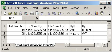
4.10 The Spot Types File
The Spot Types file (STF) is another optional tab-delimited text file that allows you to identify
different types of probes from the entries appearing in the gene list. It is especially useful for
identifying different types of control probes. The STF is used to set the control status of each probe
on the arrays so that plots may highlight different types of spots in an appropriate way. It is typically
used to distinguish control probes from regular probes corresponding to genes, and to distinguish
positive from negative controls, ratio from calibration controls and so on. The STF should have a
SpotType column giving the names of the different spot-types. One or more other columns should
have the same names as columns in the gene list and should contain patterns or regular expressions
sufficient to identify the spot-type. Any other columns are assumed to contain plotting attributes,
such as colors or symbols, to be associated with the spot-types. There is one row for each spot-type
to be distinguished.
The STF uses simplified regular expressions to match patterns. For example, AA* means any
string starting with AA, *AA means any code ending with AA, AA means exactly these two letters,
*AA* means any string containing AA, AA. means AA followed by exactly one other character and
AA\. means exactly AA followed by a period and no other characters. For those familiar with regular
expressions, any other regular expressions are allowed but the codes ^ for beginning of string and
$ for end of string should be excluded. Note that the patterns are matched sequentially from first
to last, so more general patterns should be included first. The first row should specify the default
spot-type and should have pattern * for all the pattern-matching columns.
Here is a short STF appropriate for the ApoAI data:
22
In this example, the columns ID and Name are found in the gene-list and contain patterns to match.
The asterisks are wildcards which can represent anything. Be careful to use upper or lower case as
appropriate and don’t insert any extra spaces. The remaining column gives colors to be associated
with the different types of points. This code assumes of that the probe annotation data.frame includes
columns ID and Name. This is usually so if GenePix has been used for the image analysis, but other
image analysis software may use other column names.
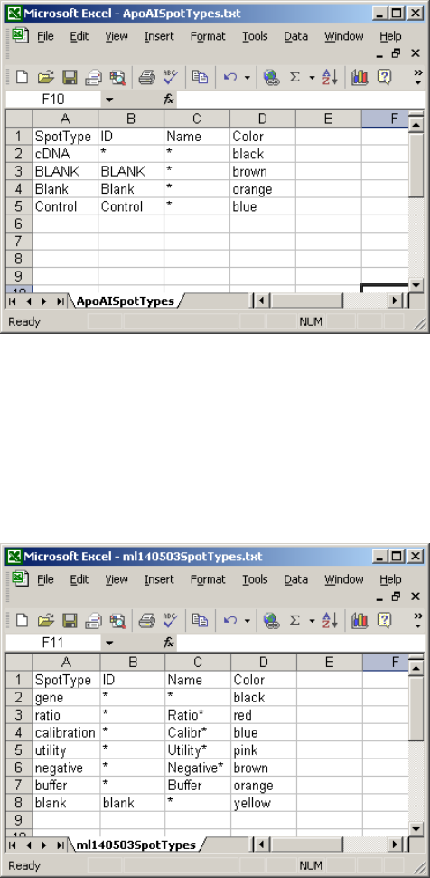
Here is a STF below appropriate for arrays with Lucidea Universal ScoreCard control spots.
If the STF has default name SpotTypes.txt then it can be read using
> spottypes <- readSpotTypes()
It is typically used as an argument to the controlStatus() function to set the status of each spot on
the array, for example
> RG$genes$Status <- controlStatus(spottypes, RG)
23
Chapter 5
Quality Assessment
An essential step in the analysis of any microarray data is to check the quality of the data from the
arrays. For two-color array data, an essential step is to view the MA-plots of the unnormalized data
for each array. The plotMD() function produces plots for individual arrays [27]. The plotMA3by2()
function gives an easy way to produce MA-plots for all the arrays in a large experiment. This
functions writes plots to disk as png files, 6 plots to a page.
The usefulness of MA-plots is enhanced by highlighting various types of control probes on the
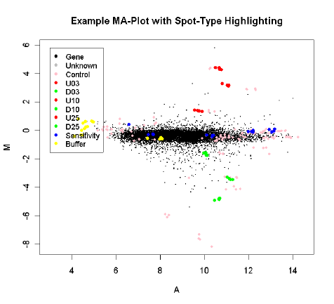
arrays, and this is facilitated by the controlStatus() function. The following is an example MA-Plot
for an Incyte array with various spike-in and other controls. (Data courtesy of Dr Steve Gerondakis,
Walter and Eliza Hall Institute of Medical Research.) The data shows high-quality data with long
comet-like pattern of non-differentially expressed probes and a small proportion of highly differen-
tially expressed probes. The plot was produced using
> spottypes <- readSpotTypes()
> RG$genes$Status <- controlStatus(spottypes, RG)
> plotMD(RG)
The array includes spike-in ratio controls which are 3-fold, 10-fold and 25-fold up and down regulated,
as well as non-differentially expressed sensitivity controls and negative controls.
24
The background intensities are also a useful guide to the quality characteristics of each array.
Boxplots of the background intensities from each array
> boxplot(data.frame(log2(RG$Gb)),main="Green background")
> boxplot(data.frame(log2(RG$Rb)),main="Red background")
will highlight any arrays unusually with high background intensities.
Spatial heterogeneity on individual arrays can be highlighted by examining imageplots of the
background intensities, for example
> imageplot(log2(RG$Gb[,1]),RG$printer)
plots the green background for the first array. The function imageplot3by2() gives an easy way to
automate the production of plots for all arrays in an experiment.
If the plots suggest that some arrays are of lesser quality than others, it may be useful to estimate
array quality weights to be used in the linear model analysis, see Section 14.
25
Chapter 6
Pre-Processing Two-Color Data
6.1 Background Correction
The default background correction action is to subtract the background intensity from the fore-
ground intensity for each spot. If the RGList object has not already been background corrected, then
normalizeWithinArrays will do this by default. Hence
> MA <- normalizeWithinArrays(RG)
is equivalent to
> RGb <- backgroundCorrect(RG, method="subtract")
> MA <- normalizeWithinArrays(RGb)
However there are many other background correction options which may be preferable in certain
situations, see Ritchie et al [26].
For the purpose of assessing differential expression, we often find
> RG <- backgroundCorrect(RG, method="normexp", offset=50)
to be preferable to the simple background subtraction when using output from most image analysis
programs. This method adjusts the foreground adaptively for the background intensities and results
in strictly positive adjusted intensities, i.e., negative or zero corrected intensities are avoided. The
use of an offset damps the variation of the log-ratios for very low intensities spots towards zero.
To illustrate some differences between the different background correction methods we consider
one cDNA array which was self-self hybridized, i.e., the same RNA source was hybridized to both
channels. For this array there is no actual differential expression. The array was printed with a
human 10.5k library and hybridized with Jurkatt RNA on both channels. (Data courtesy Andrew
Holloway and Dileepa Diyagama, Peter MacCallum Cancer Centre, Melbourne.) The array included
a selection of control spots which are highlighted on the plots. Of particular interest are the spike-in
ratio controls which should show up and down fold changes of 3 and 10. The first plot displays
data acquired with GenePix software and background corrected by subtracting the median local
background, which is the default with GenePix data. The plot shows the typical wedge shape with
fanning of the M-values at low intensities. The range of observed M-values dominates the spike-in
ratio controls. The are also 1148 spots not shown on the plot because the background corrected
intensities were zero or negative.
26
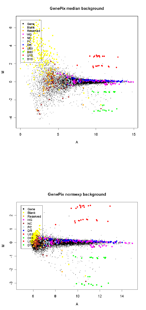
The second plot shows the same array background corrected with method="normexp" and offset=50.
The spike-in ratio controls now standout clearly from the range of the M-values. All spots on the
array are shown on the plot because there are now no missing M-values.
The third plot shows the same array quantified with SPOT software and with “morph” background
subtracted. This background estimator produces a similar effect to that with normexp.
27
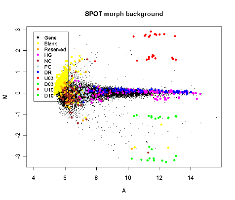
The effect of using “morph” background or using method="normexp" with an offset is to stabilize the
variability of the M-values as a function of intensity. The empirical Bayes methods implemented in
the limma package for assessing differential expression will yield most benefit when the variabilities
are as homogeneous as possible between genes. This can best be achieved by reducing the dependence
of variability on intensity as far as possible [26].
6.2 Within-Array Normalization
Limma implements a range of normalization methods for spotted microarrays. Smyth and Speed
[33] describe some of the most commonly used methods. The methods may be broadly classified
into methods which normalize the M-values for each array separately (within-array normalization)
and methods which normalize intensities or log-ratios to be comparable across arrays (between-array
normalization). This section discusses mainly within-array normalization, which all that is usually
required for the traditional log-ratio analysis of two-color data. Between-array normalization is
discussed further in Section 6.3.
Print-tip loess normalization [44] is the default normalization method and can be performed by
> MA <- normalizeWithinArrays(RG)
There are some notable cases where this is not appropriate. For example, Agilent arrays do not have
print-tip groups, so one should use global loess normalization instead:
> MA <- normalizeWithinArrays(RG, method="loess")
Print-tip loess is also unreliable for small arrays with less than, say, 150 spots per print-tip group.
Even larger arrays may have particular print-tip groups which are too small for print-tip loess nor-
malization if the number of spots with non-missing M-values is small for one or more of the print-tip
groups. In these cases one should either use global "loess" normalization or else use robust spline
normalization
> MA <- normalizeWithinArrays(RG, method="robustspline")
28
which is an empirical Bayes compromise between print-tip and global loess normalization, with 5-
parameter regression splines used in place of the loess curves.
Loess normalization assumes that the bulk of the probes on the array are not differentially
expressed. It doesn’t assume that there are equal numbers of up and down regulated genes or that
differential expression is symmetric about zero, provided that the loess fit is implemented in a robust
fashion, but it is necessary that there be a substantial body of probes which do not change expression
levels. Oshlack et al [19] show that loess normalization can tolerate up to about 30% asymmetric
differential expression while still giving good results. This assumption can be suspect for boutique
arrays where the total number of unique genes on the array is small, say less than 150, particularly if
these genes have been selected for being specifically expressed in one of the RNA sources. In such a
situation, the best strategy is to include on the arrays a series of non-differentially expressed control
spots, such as a titration series of whole-library-pool spots, and to use the up-weighting method
discussed below [19]. A whole-library-pool means that one makes a pool of a library of probes, and
prints spots from the pool at various concentrations [43]. The library should be sufficiently large
than one can be confident that the average of all the probes is not differentially expressed. The larger
the library the better. Good results have been obtained with library pools with as few as 500 clones.
In the absence of such control spots, normalization of boutique arrays requires specialist advice.
Any spot quality weights found in RG will be used in the normalization by default. This means
for example that spots with zero weight (flagged out) will not influence the normalization of other
spots. The use of spot quality weights will not however result in any spots being removed from the
data object. Even spots with zero weight will be normalized and will appear in the output object,
such spots will simply not have any influence on the other spots. If you do not wish the spot quality
weights to be used in the normalization, their use can be over-ridden using
> MA <- normalizeWithinArrays(RG, weights=NULL)
The output object MA will still contain any spot quality weights found in RG, but these weights are
not used in the normalization step.
It is often useful to make use of control spots to assist the normalization process. For example,
if the arrays contain a series of spots which are known in advance to be non-differentially expressed,
these spots can be given more weight in the normalization process. Spots which are known in advance
to be differentially expressed can be down-weighted. Suppose for example that the controlStatus()
has been used to identify spike-in spots which are differentially expressed and a titration series of
whole-library-pool spots which should not be differentially expressed. Then one might use
> w <- modifyWeights(RG$weights, RG$genes$Status, c("spikein","titration"), c(0,2))
> MA <- normalizeWithinArrays(RG, weights=w)
to give zero weight to the spike-in spots and double weight to the titration spots. This process is
automated by the "control" normalization method, for example
> csi <- RG$genes$Status=="titration"
> MA <- normalizeWithinArrays(RG, method="control", controlspots=csi)
In general, csi is an index vector specifying the non-differentially expressed control spots [19].
The idea of up-weighting the titration spots is in the same spirit as the composite normalization
method proposed by [43] but is more flexible and generally applicable. The above code assumes that
RG already contains spot quality weights. If not, one could use
> w <- modifyWeights(array(1,dim(RG)), RG$genes$Status, c("spikein","titration"), c(0,2))
> MA <- normalizeWithinArrays(RG, weights=w)
29
instead.
Limma contains some more sophisticated normalization methods. In particular, some between-
array normalization methods are discussed in Section 6.3 of this guide.
6.3 Between-Array Normalization
This section explores some of the methods available for between-array normalization of two-color
arrays. A feature which distinguishes most of these methods from within-array normalization is the
focus on the individual red and green intensity values rather than merely on the log-ratios. These
methods might therefore be called individual channel or separate channel normalization methods.
Individual channel normalization is typically a prerequisite to individual channel analysis methods
such as that provided by lmscFit(). Further discussion of the issues involved is given by [46].
This section shows how to reproduce some of the results given in [46]. The Apoa1 data set from
Section 16.2 will be used to illustrate these methods. We assume that the Apoa1 data has been
loaded and background corrected as follows:
> load("Apoa1.RData")
An important issue to consider before normalizing between arrays is how background correction
has been handled. For between-array normalization to be effective, it is important to avoid missing
values in log-ratios which might arise from negative or zero corrected intensities. The function
backgroundCorrect() gives a number of useful options. For the purposes of this section, the data has
been corrected using the "minimum" method:
> RG.b <- backgroundCorrect(RG,method="minimum")
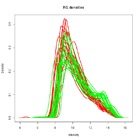
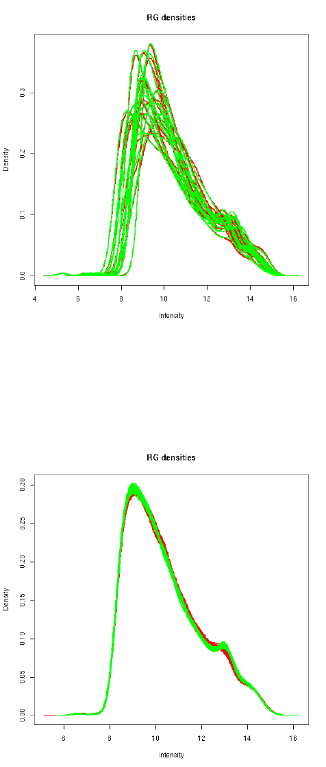
plotDensities displays smoothed empirical densities for the individual green and red channels
on all the arrays. Without any normalization there is considerable variation between both channels
and between arrays:
> plotDensities(RG.b)
30
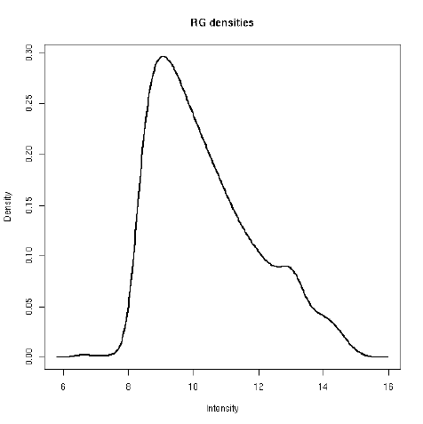
After loess normalization of the M-values for each array the red and green distributions become
essentially the same for each array, although there is still considerable variation between arrays:
> MA.p <-normalizeWithinArrays(RG.b)
> plotDensities(MA.p)
Loess normalization doesn’t affect the A-values. Applying quantile normalization to the A-values
makes the distributions essentially the same across arrays as well as channels:
> MA.pAq <- normalizeBetweenArrays(MA.p, method="Aquantile")
> plotDensities(MA.pAq)
31
Applying quantile normalization directly to the individual red and green intensities produces a
similar result but is somewhat noisier:
> MA.q <- normalizeBetweenArrays(RG.b, method="quantile")
> plotDensities(MA.q, col="black")
Warning message:
number of groups=2 not equal to number of col in: plotDensities(MA.q, col = "black")
There are other between-array normalization methods not explored here. For example normalizeBetweenArrays
with method="vsn" gives an interface to the variance-stabilizing normalization methods of the vsn
package.
6.4 Using Objects from the marray Package
The package marray is a well known R package for pre-processing of two-color microarray data.
Marray provides functions for reading, normalization and graphical display of data. Marray and
limma are both descendants of the earlier and path-breaking sma package available from http://www.
stat.berkeley.edu/users/terry/zarray/Software/smacode.html but limma has maintained and
built upon the original data structures whereas marray has converted to a fully formal data class
representation. For this reason, Limma is backwardly compatible with sma while marray is not.
Normalization functions in marray focus on a flexible approach to location and scale normalization
of M-values, rather than the within and between-array approach of limma. Marray provides some
normalization methods which are not in limma including 2-D loess normalization and print-tip-scale
normalization. Although there is some overlap between the normalization functions in the two pack-
ages, both providing print-tip loess normalization, the two approaches are largely complementary.
Marray also provides highly developed functions for graphical display of two-color microarray data.
Read functions in marray produce objects of class marrayRaw while normalization produces objects
of class marrayNorm. Objects of these classes may be converted to and from limma data objects using
32
the convert package. marrayRaw objects may be converted to RGList objects and marrayNorm objects
to MAList objects using the as function. For example, if Data is an marrayNorm object then
> library(convert)
> MA <- as(Data, "MAList")
converts to an MAList object.
marrayNorm objects can also be used directly in limma without conversion, and this is generally
recommended. If Data is an marrayNorm object, then
> fit <- lmFit(Data, design)
fits a linear model to Data as it would to an MAList object. One difference however is that the marray
read functions tend to populate the maW slot of the marrayNorm object with qualitative spot quality
flags rather than with quantitative non-negative weights, as expected by limma. If this is so then
one may need
> fit <- lmFit(Data, design, weights=NULL)
to turn off use of the spot quality weights.
33
Chapter 7
Filtering unexpressed probes
Sometimes the expression profiling platform (microarray or RNA-seq) includes probes or genes that
do not appear to be expressed to a worthwhile degree in any of the RNA samples being compared.
This might occur for example for genes that are not expressed in any of the cell types being profiled
in the experiment. Genes that are never expressed are, by definition, not differentially expressed, and
such genes are unlikely to be of biological interest in a study. In these cases, it may be possible to
simplify the differential expression analysis by removing such genes from further consideration early
in the analysis. Whether this is worthwhile and how it is done depends on the expression platform.
For two-color microarrays, it is usual to use all the available probes during the background
correction and normalization steps. Control probes that don’t correspond to genes are usually then
removed before the differential expression analysis steps, but no other filtering is done.
For single-channel microarrays, it often is worthwhile to identify and filter unexpressed probes.
Some microarray platforms, including Illumina, Agilent and Affymetrix arrays, include control probes
from which the background intensity corresponding to unexpressed probes can be estimated. In such
cases, it may be useful to keep probes that are expressed above background on at least k arrays, where
k is the smallest number of replicates assigned to any of the treatment combinations. Such filtering
is done before the linear modeling and empirical Bayes steps but after normalization. Section 17.3.4
gives an example of filtering with Illumina arrays and Section 17.4.6 gives an example with Agilent
arrays.
If background control probes are not available, an alternative single-channel approach is to filter
probes based on their average log-expression values (AveExpr) as computed by lmFit and stored as
Amean. A histogram of the Amean values and a sigma vs Amean plot may help identify a cutoff below
which Amean values can be filtered:
fit <- lmFit(y, design)
hist(fit$Amean)
plotSA(fit)
Then empirical Bayes and downstream analyses can be conducted on the filtered fit object:
keep <- fit$Amean > CutOff
fit2 <- eBayes(fit[keep,], trend=TRUE)
plotSA(fit2)
Filtering is most important for RNA-seq. For RNA-seq data is important to filter out genes
or exons that are never detected or have very small counts. An effective method is to keep genes
or exons that have a worthwhile count, say 5–10 or more, in at least k arrays, where k is the
34
smallest number of replicates assigned to any of the treatment combinations. The edgeR package
provides the filterByExpr function to identify genes or exons for filtering, as will be outlined briefly
in Section 15.3.
35
Chapter 8
Linear Models Overview
8.1 Introduction
The package limma uses an approach called linear models to analyze designed microarray experiments.
This approach allows very general experiments to be analyzed just as easily as a simple replicated
experiment. The approach is outlined in [35, 45]. The approach requires one or two matrices to
be specified. The first is the design matrix which indicates in effect which RNA samples have been
applied to each array. The second is the contrast matrix which specifies which comparisons you
would like to make between the RNA samples. For very simple experiments, you may not need to
specify the contrast matrix.
The philosophy of the approach is as follows. You have to start by fitting a linear model to
your data which fully models the systematic part of your data. The model is specified by the design
matrix. Each row of the design matrix corresponds to an array in your experiment and each column
corresponds to a coefficient that is used to describe the RNA sources in your experiment. With
Affymetrix or single-channel data, or with two-color with a common reference, you will need as
many coefficients as you have distinct RNA sources, no more and no less. With direct-design two-
color data you will need one fewer coefficient than you have distinct RNA sources, unless you wish
to estimate a dye-effect for each gene, in which case the number of RNA sources and the number of
coefficients will be the same. Any set of independent coefficients will do, providing they describe all
your treatments. The main purpose of this step is to estimate the variability in the data, hence the
systematic part needs to be modeled so it can be distinguished from random variation.
In practice the requirement to have exactly as many coefficients as RNA sources is too restrictive
in terms of questions you might want to answer. You might be interested in more or fewer comparisons
between the RNA source. Hence the contrasts step is provided so that you can take the initial
coefficients and compare them in as many ways as you want to answer any questions you might have,
regardless of how many or how few these might be.
If you have data from Affymetrix experiments, from single-channel spotted microarrays or from
spotted microarrays using a common reference, then linear modeling is the same as ordinary analysis
of variance or multiple regression except that a model is fitted for every gene. With data of this type
you can create design matrices as one would do for ordinary modeling with univariate data. If you
have data from spotted microarrays using a direct design, i.e., a connected design with no common
reference, then the linear modeling approach is very powerful but the creation of the design matrix
may require more statistical knowledge.
For statistical analysis and assessing differential expression, limma uses an empirical Bayes method
36
to moderate the standard errors of the estimated log-fold changes. This results in more stable
inference and improved power, especially for experiments with small numbers of arrays [35, 21]. For
arrays with within-array replicate spots, limma uses a pooled correlation method to make full use of
the duplicate spots [32].
8.2 Single-Channel Designs
Affymetrix data will usually be normalized using the affy package. We will assume here that the
data is available as an ExpressionSet object called eset. Such an object will have an slot containing
the log-expression values for each gene on each array which can be extracted using exprs(eset).
Affymetrix and other single-channel microarray data may be analyzed very much like ordinary linear
models or anova models. The difference with microarray data is that it is almost always necessary
to extract particular contrasts of interest and so the standard parametrizations provided for factors
in R are not usually adequate.
There are many ways to approach the analysis of a complex experiment in limma. A straightfor-
ward strategy is to set up the simplest possible design matrix and then to extract from the fit the
contrasts of interest.
Suppose that there are three RNA sources to be compared. Suppose that the first three arrays
are hybridized with RNA1, the next two with RNA2 and the next three with RNA3. Suppose that
all pair-wise comparisons between the RNA sources are of interest. We assume that the data has
been normalized and stored in an ExpressionSet object, for example by
> data <- ReadAffy()
> eset <- rma(data)
An appropriate design matrix can be created and a linear model fitted using
> design <- model.matrix(~ 0+factor(c(1,1,1,2,2,3,3,3)))
> colnames(design) <- c("group1", "group2", "group3")
> fit <- lmFit(eset, design)
To make all pair-wise comparisons between the three groups the appropriate contrast matrix can be
created by
> contrast.matrix <- makeContrasts(group2-group1, group3-group2, group3-group1, levels=design)
> fit2 <- contrasts.fit(fit, contrast.matrix)
> fit2 <- eBayes(fit2)
A list of top genes differential expressed in group2 versus group1 can be obtained from
> topTable(fit2, coef=1, adjust="BH")
The outcome of each hypothesis test can be assigned using
> results <- decideTests(fit2)
A Venn diagram showing numbers of genes significant in each comparison can be obtained from
> vennDiagram(results)
37
8.3 Common Reference Designs
Now consider two-color microarray experiments in which a common reference has been used on all
the arrays. Such experiments can be analyzed very similarly to Affymetrix experiments except that
allowance must be made for dye-swaps. The simplest method is to setup the design matrix using
the modelMatrix() function and the targets file. As an example, we consider part of an experiment
conducted by Jo¨elle Michaud, Catherine Carmichael and Dr Hamish Scott at the Walter and Eliza
Hall Institute to compare the effects of transcription factors in a human cell line. The targets file is
as follows:
> targets <- readTargets("runxtargets.txt")
> targets
SlideNumber Cy3 Cy5
1 2144 EGFP AML1
2 2145 EGFP AML1
3 2146 AML1 EGFP
4 2147 EGFP AML1.CBFb
5 2148 EGFP AML1.CBFb
6 2149 AML1.CBFb EGFP
7 2158 EGFP CBFb
8 2159 CBFb EGFP
9 2160 EGFP AML1.CBFb
10 2161 AML1.CBFb EGFP
11 2162 EGFP AML1.CBFb
12 2163 AML1.CBFb EGFP
13 2166 EGFP CBFb
14 2167 CBFb EGFP
In the experiment, green fluorescent protein (EGFP) has been used as a common reference. An
adenovirus system was used to transport various transcription factors into the nuclei of HeLa cells.
Here we consider the transcription factors AML1, CBFbeta or both. A simple design matrix was
formed and a linear model fit:
> design <- modelMatrix(targets,ref="EGFP")
> design
AML1 AML1.CBFb CBFb
1 1 0 0
2 1 0 0
3 -1 0 0
4 0 1 0
5 0 1 0
6 0 -1 0
7 0 0 1
8 0 0 -1
9 0 1 0
10 0 -1 0
11 0 1 0
12 0 -1 0
13 0 0 1
14 0 0 -1
> fit <- lmFit(MA, design)
It is of interest to compare each of the transcription factors to EGFP and also to compare the
combination transcription factor with AML1 and CBFb individually. An appropriate contrast matrix
was formed as follows:
38
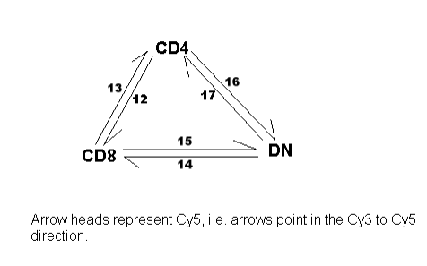
> contrast.matrix <- makeContrasts(AML1,CBFb,AML1.CBFb,AML1.CBFb-AML1,AML1.CBFb-CBFb,
+ levels=design)
> contrast.matrix
AML1 CBFb AML1.CBFb AML1.CBFb - AML1 AML1.CBFb - CBFb
AML1 1 0 0 -1 0
AML1.CBFb 0 0 1 1 1
CBFb 0 1 0 0 -1
The linear model fit can now be expanded and empirical Bayes statistics computed:
> fit2 <- contrasts.fit(fit, contrasts.matrix)
> fit2 <- eBayes(fit2)
8.4 Direct Two-Color Designs
Two-color designs without a common reference require the most statistical knowledge to choose
the appropriate design matrix. A direct design is one in which there is no single RNA source
which is hybridized to every array. As an example, we consider an experiment conducted by Dr
Mireille Lahoud at the Walter and Eliza Hall Institute to compare gene expression in three different
populations of dendritic cells (DC).
This experiment involved six cDNA microarrays in three dye-swap pairs, with each pair used to
compare two DC types. The design is shown diagrammatically above. The targets file was as
follows:
> targets
SlideNumber FileName Cy3 Cy5
ml12med 12 ml12med.spot CD4 CD8
ml13med 13 ml13med.spot CD8 CD4
ml14med 14 ml14med.spot DN CD8
ml15med 15 ml15med.spot CD8 DN
ml16med 16 ml16med.spot CD4 DN
ml17med 17 ml17med.spot DN CD4
There are many valid choices for a design matrix for such an experiment and no single correct
choice. We chose to setup the design matrix as follows:
> design <- modelMatrix(targets, ref="CD4")
Found unique target names:
CD4 CD8 DN
39
> design
CD8 DN
ml12med 1 0
ml13med -1 0
ml14med 1 -1
ml15med -1 1
ml16med 0 1
ml17med 0 -1
In this design matrix, the CD8 and DN populations have been compared back to the CD4 population.
The coefficients estimated by the linear model will correspond to the log-ratios of CD8 vs CD4 (first
column) and DN vs CD4 (second column).
After appropriate normalization of the expression data, a linear model was fit using
> fit <- lmFit(MA, design)
The linear model can now be interrogated to answer any questions of interest. For this experiment
it was of interest to make all pairwise comparisons between the three DC populations. This was
accomplished using the contrast matrix
> contrast.matrix <- cbind("CD8-CD4"=c(1,0),"DN-CD4"=c(0,1),"CD8-DN"=c(1,-1))
> rownames(contrast.matrix) <- colnames(design)
> contrast.matrix
CD8-CD4 DN-CD4 CD8-DN
CD8 1 0 1
DN 0 1 -1
The contrast matrix can be used to expand the linear model fit and then to compute empirical Bayes
statistics:
> fit2 <- contrasts.fit(fit, contrast.matrix)
> fit2 <- eBayes(fit2)
40

Chapter 9
Single-Channel Experimental Designs
9.1 Introduction
Unlike the early days of microarrays, most data is now of the single channel type. Single channel
data is generated from popular microarray technologies such as Affymetrix, Illumina or Agilent. The
new technology of RNA-seq also generates single channel data, so everything in this chapter can be
applied to RNA-seq analyses when the data has been pre-processed using the voom function [13].
Single-channel data may be analyzed very much like ordinary univariate linear models or analysis
of variance. The difference with microarray data is that it is almost always necessary to extract
particular contrasts of interest and so the standard parametrizations provided for factors in R are
not usually adequate.
We will assume for our examples here that the data has been suitably pre-processed normalized
and is available as an ExpressionSet or EList object called eset. Such an object will have an
slot containing the log-expression values for each gene on each array which can be extracted using
exprs(eset).
9.2 Two Groups
The simplest possible single channel experiment is to compare two groups. Suppose that we wish to
compare two wild type (Wt) mice with three mutant (Mu) mice:
FileName Target
File1 WT
File2 WT
File3 Mu
File4 Mu
File5 Mu
There are two different ways to form the design matrix. We can either
1. create a design matrix which includes a coefficient for the mutant vs wild type difference, or
2. create a design matrix which includes separate coefficients for wild type and mutant mice and
then extract the difference as a contrast.
41
For the first approach, the treatment-contrasts parametrization, the design matrix should be as
follows:
> design
WT MUvsWT
Array1 1 0
Array2 1 0
Array3 1 1
Array4 1 1
Array5 1 1
Here the first coefficient estimates the mean log-expression for wild type mice and plays the role
of an intercept. The second coefficient estimates the difference between mutant and wild type.
Differentially expressed genes can be found by
> fit <- lmFit(eset, design)
> fit <- eBayes(fit)
> topTable(fit, coef="MUvsWT", adjust="BH")
where eset is an ExpressionSet or matrix object containing the log-expression values. For the second
approach, the design matrix should be
WT MU
Array1 1 0
Array2 1 0
Array3 0 1
Array4 0 1
Array5 0 1
Differentially expressed genes can be found by
> fit <- lmFit(eset, design)
> cont.matrix <- makeContrasts(MUvsWT=MU-WT, levels=design)
> fit2 <- contrasts.fit(fit, cont.matrix)
> fit2 <- eBayes(fit2)
> topTable(fit2, adjust="BH")
For the first approach, the treatment-contrasts parametrization, the design matrix can be com-
puted by
> design <- cbind(WT=1,MUvsWT=c(0,0,1,1,1))
or by
> Group <- factor(targets$Target, levels=c("WT","Mu"))
> design <- model.matrix(~Group)
> colnames(design) <- c("WT","MUvsWT")
For the second approach, the group-means parametrization, the design matrix can be computed by
> design <- cbind(WT=c(1,1,0,0,0),MU=c(0,0,1,1,1))
or by
> design <- model.matrix(~0+Group)
> colnames(design) <- c("WT","MU")
42

9.3 Several Groups
The above approaches for two groups extend easily to any number of groups. Suppose that three
RNA targets to be compared. Suppose that the three targets are called “RNA1”, “RNA2” and
“RNA3” and that the column targets Target indicates which one was hybridized to each array. An
appropriate design matrix can be created using
> f <- factor(targets$Target, levels=c("RNA1","RNA2","RNA3"))
> design <- model.matrix(~0+f)
> colnames(design) <- c("RNA1","RNA2","RNA3")
To make all pair-wise comparisons between the three groups one could proceed
> fit <- lmFit(eset, design)
> contrast.matrix <- makeContrasts(RNA2-RNA1, RNA3-RNA2, RNA3-RNA1,
+ levels=design)
> fit2 <- contrasts.fit(fit, contrast.matrix)
> fit2 <- eBayes(fit2)
A list of top genes for RNA2 versus RNA1 can be obtained from
> topTable(fit2, coef=1, adjust="BH")
The outcome of each hypothesis test can be assigned using
> results <- decideTests(fit2)
A Venn diagram showing numbers of genes significant in each comparison can be obtained from
> vennDiagram(results)
The statistic fit2 F and the corresponding fit2 F.p.value combine the three pair-wise compar-
isons into one F-test. This is equivalent to a one-way ANOVA for each gene except that the residual
mean squares have been moderated between genes. To find genes which vary between the three RNA
targets in any way, look for genes with small p-values. To find the top 30 genes:
> topTable(fit2, number=30)
Here, with the coef argument not specified, topTable will test all coefficients or contrasts found in
the linear model object equal to zero. When two or more contrasts are present, then the F-tests for
those contrasts are reported. In this case, fit2 contains three contrasts, so F-tests on 3 degrees of
freedom (df) will be reported.
9.4 Additive Models and Blocking
9.4.1 Paired Samples
Paired samples occur when we compare two treatments and each sample given one treatment is
naturally paired with a particular sample given the other treatment. This is a special case of blocking
with blocks of size two. The classical test associated with this situation is the paired t-test.
Suppose an experiment is conducted to compare a new treatment (T) with a control (C). Six
dogs are used from three sib-ships. For each sib-pair, one dog is given the treatment while the other
dog is a control. This produces the targets frame:
43

FileName SibShip Treatment
File1 1 C
File2 1 T
File3 2 C
File4 2 T
File5 3 C
File6 3 T
A moderated paired t-test can be computed by allowing for sib-pair effects in the linear model:
> SibShip <- factor(targets$SibShip)
> Treat <- factor(targets$Treatment, levels=c("C","T"))
> design <- model.matrix(~SibShip+Treat)
> fit <- lmFit(eset, design)
> fit <- eBayes(fit)
> topTable(fit, coef="TreatT")
9.4.2 Blocking
The above approach used for paired samples can be applied in any situation where there are batch
effects or where the experiment has been conducted in blocks. The treatments can be adjusted for
differences between the blocks by using a model formula of the form:
> design <- model.matrix(~Block+Treatment)
In this type of analysis, the treatments are compared only within each block.
9.5 Interaction Models: 2 × 2 Factorial Designs
9.5.1 Questions of Interest
Factorial designs are those where more than one experimental dimension is being varied and each
combination of treatment conditions is observed. Suppose that cells are extracted from wild type and
mutant mice and these cells are either stimulated (S) or unstimulated (U). RNA from the treated
cells is then extracted and hybridized to a microarray. We will assume for simplicity that the arrays
are single-color arrays such as Affymetrix. Consider the following targets frame:
FileName Strain Treatment
File1 WT U
File2 WT S
File3 Mu U
File4 Mu S
File5 Mu S
The two experimental dimensions or factors here are Strain and Treatment. Strain specifies the
genotype of the mouse from which the cells are extracted and Treatment specifies whether the cells
are stimulated or not. All four combinations of Strain and Treatment are observed, so this is a
factorial design. It will be convenient for us to collect the Strain/Treatment combinations into one
vector as follows:
> TS <- paste(targets$Strain, targets$Treatment, sep=".")
> TS
44
[1] "WT.U" "WT.S" "Mu.U" "Mu.S" "Mu.S"
It is especially important with a factorial design to decide what are the comparisons of interest.
We will assume here that the experimenter is interested in
1. which genes respond to stimulation in wild-type cells,
2. which genes respond to stimulation in mutant cells, and
3. which genes respond differently in mutant compared to wild-type cells.
as these are the questions which are most usually relevant in a molecular biology context. The first
of these questions relates to the WT.S vs WT.U comparison and the second to Mu.S vs Mu.U. The third
relates to the difference of differences, i.e., (Mu.S-Mu.U)-(WT.S-WT.U), which is called the interaction
term.
9.5.2 Analysing as for a Single Factor
We describe first a simple way to analyze this experiment using limma commands in a similar way to
that in which two-sample designs were analyzed. Then we will go on to describe the more classical
statistical approaches using factorial model formulas. All the approaches considered are equivalent
and yield identical bottom-line results. The most basic approach is to fit a model with a coefficient
for each of the four factor combinations and then to extract the comparisons of interest as contrasts:
> TS <- factor(TS, levels=c("WT.U","WT.S","Mu.U","Mu.S"))
> design <- model.matrix(~0+TS)
> colnames(design) <- levels(TS)
> fit <- lmFit(eset, design)
This fits a model with four coefficients corresponding to WT.U, WT.S, Mu.U and Mu.S respectively. Our
three contrasts of interest can be extracted by
> cont.matrix <- makeContrasts(
+ SvsUinWT=WT.S-WT.U,
+ SvsUinMu=Mu.S-Mu.U,
+ Diff=(Mu.S-Mu.U)-(WT.S-WT.U),
+ levels=design)
> fit2 <- contrasts.fit(fit, cont.matrix)
> fit2 <- eBayes(fit2)
We can use topTable() to look at lists of differentially expressed genes for each of three contrasts, or
else
> results <- decideTests(fit2)
> vennDiagram(results)
to look at all three contrasts simultaneously.
This approach is recommended for most users, because the contrasts that are being tested are
formed explicitly.
45
9.5.3 A Nested Interaction Formula
Model formulas in R are very flexible, and offer lots of possible shortcuts for setting up the design
matrix. However they also require a high level of statistical understanding in order to use reliably,
and they are not completely described in the main R documentation. If we only wanted to test the
first two questions above, an easy to setup the design matrix would be to use a nested interaction
term:
> Strain <- factor(targets$Strain, levels=c("WT","Mu"))
> Treatment <- factor(targets$Treatment, levels=c("U","S"))
> design <- model.matrix(~Strain+Strain:Treatment)
> colnames(design)
[1] "(Intercept)" "StrainMu" "StrainWT:TreatmentS" "StrainMu:TreatmentS"
The first term in the model formula is an effect for Strain. This introduces an intercept column to
the design matrix, which estimates the average log-expression level for wild-type unstimulated cells,
and a column for Strain which estimates the mutant vs wild-type difference in the unstimulated
state. The second term in the model formula represents the interaction between stimulation and
strain. Because there is no main effect for treatment in the model, the interaction is fitted in a
nested sense. It introduces a third and a fourth column to the design matrix which represent the
effect of stimulation for wild-type and for mutant mice respectively, exactly the same as the contrasts
SvsUinWT and SvsUinMu define in the previous section. After
> fit <- lmFit(eset, design)
> fit <- eBayes(fit)
then
> topTable(fit, coef=3)
will find those genes responding to stimulation in wild-type mice, and
> topTable(fit, coef=4)
will find those genes responding to stimulation in mutant mice. Finally, we could extract the inter-
action contrast Diff considered above by
> fit2 <- contrasts.fit(fit, c(0,0,-1,1))
> fit2 <- eBayes(fit2)
> topTable(fit2)
This finds genes that respond differently to the stimulus in mutant vs wild-type mice.
9.5.4 Classic Interaction Models
The analysis of factorial designs has a long history in statistics and a system of factorial model
formulas has been developed to facilitate the analysis of complex designs. It is important to un-
derstand though that the above three molecular biology questions do not correspond to any of the
classic parametrizations used in statistics for factorial designs. Hence we generally recommend the
approaches already considered above for microarray analysis.
Suppose for example that we proceed in the usual statistical way,
> design <- model.matrix(~Strain*Treatment)
46

This creates a design matrix which defines four coefficients with the following interpretations:
Coefficient Comparison Interpretation
Intercept WT.U Baseline level of unstimulated WT
StrainMu Mu.U-WT.U Difference between unstimulated strains
TreatmentS WT.S-WT.U Stimulation effect for WT
StrainMu:TreatmentS (Mu.S-Mu.U)-(WT.S-WT.U) Interaction
This is called the treatment-contrast parametrization. Notice that one of our comparisons of interest,
Mu.S-Mu.U, is not represented and instead the comparison Mu.U-WT.U, which might not be of direct
interest, is included. We need to use contrasts to extract all the comparisons of interest:
> fit <- lmFit(eset, design)
> cont.matrix <- cbind(SvsUinWT=c(0,0,1,0),SvsUinMu=c(0,0,1,1),Diff=c(0,0,0,1))
> fit2 <- contrasts.fit(fit, cont.matrix)
> fit2 <- eBayes(fit2)
This extracts the WT stimulation effect as the third coefficient and the interaction as the fourth
coefficient. The mutant stimulation effect is extracted as the sum of the third and fourth coefficients
of the original model. This analysis yields exactly the same results as the previous analysis.
An even more classical statistical approach to the factorial experiment would be to use the sum
to zero parametrization. In R this is achieved by
> contrasts(Strain) <- contr.sum(2)
> contrasts(Treatment) <- contr.sum(2)
> design <- model.matrix(~Strain*Treatment)
This defines four coefficients with the following interpretations:
Coefficient Comparison Interpretation
Intercept (WT.U+WT.S+Mu.U+Mu.S)/4 Grand mean
Strain1 (WT.U+WT.S-Mu.U-Mu.S)/4 Strain main effect
Treatment1 (WT.U-WT.S+Mu.U-Mu.S)/4 Treatment main effect
Strain1:Treatment1 (WT.U-WT.S-Mu.U+Mu.S)/4 Interaction
This parametrization has many appealing mathematical properties and is the classical parametriza-
tion used for factorial designs in much experimental design theory. However it defines only one
coefficient which is directly of interest to us, namely the interaction. Our three contrasts of interest
could be extracted using
> fit <- lmFit(eset, design)
> cont.matrix <- cbind(SvsUinWT=c(0,0,-2,-2),SvsUinMu=c(0,0,-2,2),Diff=c(0,0,0,4))
> fit2 <- contrasts.fit(fit, cont.matrix)
> fit2 <- eBayes(fit2)
The results will be identical to those for the previous three approaches.
The various approaches described here for the 2 × 2 factorial problem are equivalent and differ
only in the parametrization chosen for the linear model. The fitted model objects fit will differ
only in the coefficients and associated components. The residual standard deviations fit$sigma,
residual degrees of freedom fit$df.residual and all components of fit2 will be identical regardless
of parametrization used. Since the approaches are equivalent, users are free to choose whichever one
is most intuitive or convenient.
47

9.6 Time Course Experiments
9.6.1 Replicated time points
Time course experiments are those in which RNA is extracted at several time points after the onset
of some treatment or stimulation. How best to analyse a time course experiment depends on the
nature of the experiment, and especially on the number of distinct time points. We consider first
experiments with a relative small number of replicated time points. Simple time course experiments
of this type are similar to experiments with several groups covered in Section 9.3.
As an example, we consider here a two-way experiment in which time course profiles are to be
compared for two genotypes. Consider the targets frame
FileName Target
File1 wt.0hr
File2 wt.0hr
File3 wt.6hr
File4 wt.24hr
File5 mu.0hr
File6 mu.0hr
File7 mu.6hr
File8 mu.24hr
The targets are RNA samples collected from wild-type and mutant animals at 0, 6 and 24 hour time
points. This can be viewed as a factorial experiment but a simpler approach is to use the group-mean
parametrization.
> lev <- c("wt.0hr","wt.6hr","wt.24hr","mu.0hr","mu.6hr","mu.24hr")
> f <- factor(targets$Target, levels=lev)
> design <- model.matrix(~0+f)
> colnames(design) <- lev
> fit <- lmFit(eset, design)
Which genes respond at either the 6 hour or 24 hour times in the wild-type? We can find these
by extracting the contrasts between the wild-type times.
> cont.wt <- makeContrasts(
+ "wt.6hr-wt.0hr",
+ "wt.24hr-wt.6hr",
+ levels=design)
> fit2 <- contrasts.fit(fit, cont.wt)
> fit2 <- eBayes(fit2)
> topTable(fit2, adjust="BH")
Any two contrasts between the three times would give the same result. The same gene list would be
obtained had "wt.24hr-wt.0hr" been used in place of "wt.24hr-wt.6hr" for example.
Which genes respond (i.e., change over time) in the mutant?
> cont.mu <- makeContrasts(
+ "mu.6hr-mu.0hr",
+ "mu.24hr-mu.6hr",
+ levels=design)
> fit2 <- contrasts.fit(fit, cont.mu)
> fit2 <- eBayes(fit2)
> topTable(fit2, adjust="BH")
48

Which genes respond differently over time in the mutant relative to the wild-type?
> cont.dif <- makeContrasts(
+ Dif6hr =(mu.6hr-mu.0hr)-(wt.6hr-wt.0hr),
+ Dif24hr=(mu.24hr-mu.6hr)-(wt.24hr-wt.6hr),
+ levels=design)
> fit2 <- contrasts.fit(fit, cont.dif)
> fit2 <- eBayes(fit2)
> topTable(fit2, adjust="BH")
The method of analysis described in this section was used for a six-point time course experiment
on histone deacetylase inhibitors [20].
9.6.2 Many time points
Now we consider an example with many time points for each group. When there are many time
points, it is reasonable to assume that expression changes smoothly over time rather than making
discrete jumps from one time point to another. This type of time course can be analysed by fitting
a temporal trend using a regression spline or a polynomial.
Consider the following targets frame, with 32 rows:
FileName Group Time
File1 Control 1
File2 Control 2
.
.
.
.
.
.
.
.
.
File16 Control 16
File17 Treat 1
File18 Treat 2
.
.
.
.
.
.
.
.
.
File32 Treat 16
It might be reasonable to represent a time course for a particular gene in a particular condition using
a cubic spline curve with a modest number of knots. Choosing effective degrees of freedom to be in
range 3–5 is reasonable. Setup a basis for a natural regression spline:
> library(splines)
> X <- ns(targets$Time, df=5)
Then fit separate curves for the control and treatment groups:
> Group <- factor(targets$Group)
> design <- model.matrix(~Group*X)
> fit <- lmFit(y, design)
> fit <- eBayes(fit)
This creates a model with 12 parameters, with the last 5 corresponding to interaction, i.e., to
differences in the curves between groups. To detect genes with different time trends for treatment
vs control:
> topTable(fit, coef=8:12)
This conducts a moderated F-test for each gene on 5 df, which can detect very general differences
between the treatment and control curves.
Note that for this analysis, it is not necessary to have replicates, nor is it necessary for the two
treatment groups to be observed at identical time points.
49

9.7 Multi-level Experiments
We have considered paired comparisons, and we have considered comparisons between two indepen-
dent groups. There are however experiments that combine both of these types of comparisons.
Consider a single-channel experiment with the following targets frame:
FileName Subject Condition Tissue
File01 1 Diseased A
File02 1 Diseased B
File03 2 Diseased A
File04 2 Diseased B
File05 3 Diseased A
File06 3 Diseased B
File07 4 Normal A
File08 4 Normal B
File09 5 Normal A
File10 5 Normal B
File11 6 Normal A
File12 6 Normal B
This experiment involves 6 subjects, including 3 patients who have the disease and 3 normal subjects.
From each subject, we have expression profiles of two tissue types, A and B.
In analysing this experiment, we want to compare the two tissue types. This comparison can be
made within subjects, because each subject yields a value for both tissues. We also want to compare
diseased subjects to normal subjects, but this comparison is between subjects.
If we only wanted to compare the two tissue types, we could do a paired samples comparison.
If we only wanted to compared diseased to normal, we could do an ordinary two group comparison.
Since we need to make comparisons both within and between subjects, it is necessary to treat Patient
as a random effect. This can be done in limma using the duplicateCorrelation function.
The two experimental factors Condition and Tissue could be handled in many ways. Here we
will assume that it is convenient to join the two into a combined factor:
> Treat <- factor(paste(targets$Condition,targets$Tissue,sep="."))
> design <- model.matrix(~0+Treat)
> colnames(design) <- levels(Treat)
Then we estimate the correlation between measurements made on the same subject:
> corfit <- duplicateCorrelation(eset,design,block=targets$Subject)
> corfit$consensus
Then this inter-subject correlation is input into the linear model fit:
> fit <- lmFit(eset,design,block=targets$Subject,correlation=corfit$consensus)
Now we can make any comparisons between the experimental conditions in the usual way, exam-
ple:
> cm <- makeContrasts(
+ DiseasedvsNormalForTissueA = Diseased.A-Normal.A,
+ DiseasedvsNormalForTissueB = Diseased.B-Normal.B,
+ TissueAvsTissueBForNormal = Normal.B-Normal.A,
+ TissueAvsTissueBForDiseased = Diseased.B-Diseased.A,
+ levels=design)
50
Then compute these contrasts and moderated t-tests:
> fit2 <- contrasts.fit(fit, cm)
> fit2 <- eBayes(fit2)
Then
> topTable(fit2, coef="DiseasedvsNormalForTissueA")
will find those genes that are differentially expressed between the normal and diseased subjects in
the A tissue type. And so on.
This experiment has two levels of variability. First, there is the variation from person to person,
which we call the between-subject strata. Then there is the variability of repeat measurements made
on the same subject, the within-subject strata. The between-subject variation is always expected
to be larger than within-subject, because the latter is adjusted for baseline differences between the
subjects. Here the comparison between tissues can be made within subjects, and hence should
be more precise than the comparison between diseased and normal, which must be made between
subjects.
51

Chapter 10
Two-Color Experiments with a
Common Reference
10.1 Introduction
Now consider two-color microarray experiments in which a common reference has been used on all
the arrays. If the same channel has been used for the common reference throughout the experiment,
then the expression log-ratios may be analysed exactly as if they were log-expression values from a
single channel experiment. In these cases, the design matrix can be formed as for a single channel
experiment.
When the common reference is dye-swapped, the simplest method is to setup the design matrix
using the modelMatrix() function and the targets file.
10.2 Two Groups
Suppose now that we wish to compare two wild type (Wt) mice with three mutant (Mu) mice using
arrays hybridized with a common reference RNA (Ref):
FileName Cy3 Cy5
File1 Ref WT
File2 Ref WT
File3 Ref Mu
File4 Ref Mu
File5 Ref Mu
The interest here is in the comparison between the mutant and wild type mice. There are two major
ways in which this comparison can be made. We can either
1. create a design matrix which includes a coefficient for the mutant vs wild type difference, or
2. create a design matrix which includes separate coefficients for wild type and mutant mice and
then extract the difference as a contrast.
For the first approach, the design matrix should be as follows
> design
52
WTvsREF MUvsWT
Array1 1 0
Array2 1 0
Array3 1 1
Array4 1 1
Array5 1 1
Here the first coefficient estimates the difference between wild type and the reference for each probe
while the second coefficient estimates the difference between mutant and wild type. For those not
familiar with model matrices in linear regression, it can be understood in the following way. The
matrix indicates which coefficients apply to each array. For the first two arrays the fitted values
will be just the WTvsREF coefficient, which is correct. For the remaining arrays the fitted values will
be WTvsREF + MUvsWT, which is equivalent to mutant vs reference, also correct. For reasons that will
be apparent later, this is sometimes called the treatment-contrasts parametrization. Differentially
expressed genes can be found by
> fit <- lmFit(MA, design)
> fit <- eBayes(fit)
> topTable(fit, coef="MUvsWT", adjust="BH")
There is no need here to use contrasts.fit() because the comparison of interest is already built
into the fitted model. This analysis is analogous to the classical pooled two-sample t-test except that
information has been borrowed between genes.
For the second approach, the design matrix should be
WT MU
Array1 1 0
Array2 1 0
Array3 0 1
Array4 0 1
Array5 0 1
The first coefficient now represents wild-type vs the reference and the second represents mutant vs
the reference. Our comparison of interest is the difference between these two coefficients. We will
call this the group-means parametrization. Differentially expressed genes can be found by
> fit <- lmFit(MA, design)
> cont.matrix <- makeContrasts(MUvsWT=MU-WT, levels=design)
> fit2 <- contrasts.fit(fit, cont.matrix)
> fit2 <- eBayes(fit2)
> topTable(fit2, adjust="BH")
The results will be exactly the same as for the first approach.
The design matrix can be constructed
1. manually,
2. using the limma function modelMatrix(), or
3. using the built-in R function model.matrix().
Let Group be the factor defined by
> Group <- factor(c("WT","WT","Mu","Mu","Mu"), levels=c("WT","Mu"))
53

For the first approach, the treatment-contrasts parametrization, the design matrix can be computed
by
> design <- cbind(WTvsRef=1,MUvsWT=c(0,0,1,1,1))
or by
> param <- cbind(WTvsRef=c(-1,1,0),MUvsWT=c(0,-1,1))
> rownames(param) <- c("Ref","WT","Mu")
> design <- modelMatrix(targets, parameters=param)
or by
> design <- model.matrix(~Group)
> colnames(design) <- c("WTvsRef","MUvsWT")
all of which produce the same result. For the second approach, the group-means parametrization,
the design matrix can be computed by
> design <- cbind(WT=c(1,1,0,0,0),MU=c(0,0,1,1,1))
or by
> param <- cbind(WT=c(-1,1,0),MU=c(-1,0,1))
> rownames(param) <- c("Ref","WT","Mu")
> design <- modelMatrix(targets, parameters=param)
or by
> design <- model.matrix(~0+Group)
> colnames(design) <- c("WT","Mu")
all of which again produce the same result.
10.3 Several Groups
The above approaches for two groups extend easily to any number of groups. Suppose that the
experiment has been conducted to compare three RNA sources, “RNA1”, “RNA2” and “RNA3”.
For example the targets frame might be
FileName Cy3 Cy5
File1 Ref RNA1
File2 RNA1 Ref
File3 Ref RNA2
File4 RNA2 Ref
File5 Ref RNA3
For this experiment the design matrix could be formed by
> design <- modelMatrix(targets, ref="Ref")
after which the analysis would be exactly as for the equivalent single channel experiment in Sec-
tion 9.3. For example, to make all pair-wise comparisons between the three groups one could proceed
> fit <- lmFit(eset, design)
> contrast.matrix <- makeContrasts(RNA2-RNA1, RNA3-RNA2, RNA3-RNA1, levels=design)
> fit2 <- contrasts.fit(fit, contrast.matrix)
> fit2 <- eBayes(fit2)
and so on.
54

Chapter 11
Direct Two-Color Experimental
Designs
11.1 Introduction
Direct two-color designs are those in which there is no common reference, but the RNA samples are
instead compared directly by competitive hybridization on the same arrays. Direct two-color designs
can be very efficient and powerful, but they require the most statistical knowledge to choose the
appropriate design matrix.
11.2 Simple Comparisons
11.2.1 Replicate Arrays
The simplest possible microarray experiment is one with a series of replicate two-color arrays all
comparing the same two RNA sources. For a three-array experiment comparing wild type (wt) and
mutant (mu) RNA, the targets file might contain the following entries:
FileName Cy3 Cy5
File1 wt mu
File2 wt mu
File3 wt mu
A list of differentially expressed probes might be found for this experiment by
> fit <- lmFit(MA)
> fit <- eBayes(fit)
> topTable(fit)
where MA holds the normalized data. The default design matrix used here is just a single column of
ones. The experiment here measures the fold change of mutant over wild type. Genes which have
positive M-values are more highly expressed in the mutant RNA while genes with negative M-values
are more highly expressed in the wild type. The analysis is analogous to the classical single-sample
t-test except that we have used empirical Bayes methods to borrow information between genes.
55

11.2.2 Dye Swaps
A simple modification of the above experiment would be to swap the dyes for one of the arrays. The
targets file might now be
FileName Cy3 Cy5
File1 wt mu
File2 mu wt
File3 wt mu
Now the analysis would be
> design <- c(1,-1,1)
> fit <- lmFit(MA, design)
> fit <- eBayes(fit)
> topTable(fit)
Alternatively the design matrix could be set, replacing the first of the above code lines, by
> design <- modelMatrix(targets, ref="wt")
where targets is the data frame holding the targets file information.
If there are at least two arrays with each dye-orientation, then it is possible to estimate and
adjust for any probe-specific dye effects. The dye-effect is estimated by an intercept term. If the
experiment was
FileName Cy3 Cy5
File1 wt mu
File2 mu wt
File3 wt mu
File4 mu wt
then we could set
> design <- cbind(DyeEffect=1,MUvsWT=c(1,-1,1,-1))
> fit <- lmFit(MA, design)
> fit <- eBayes(fit)
The genes which show dye effects can be seen by
> topTable(fit, coef="DyeEffect")
The genes which are differentially expressed in the mutant are obtained by
> topTable(fit, coef="MUvsWT")
The fold changes and significant tests in this list are corrected for dye-effects. Including the dye-effect
in the model in this way uses up one degree of freedom which might otherwise be used to estimate
the residual variability, but it is valuable if many genes show non-negligible dye-effects.
56

11.3 A Correlation Approach to Technical Replication
In the previous sections we have assumed that all arrays are biological replicates. Now consider an
experiment in which two wild-type and two mice from the same mutant strain are compared using
two arrays for each pair of mice. The targets might be
FileName Cy3 Cy5
File1 wt1 mu1
File2 wt1 mu1
File3 wt2 mu2
File4 wt2 mu2
The first and second and third and fourth arrays are technical replicates. It would not be correct
to treat this experiment as comprising four replicate arrays because the technical replicate pairs are
not independent, in fact they are likely to be positively correlated.
One way to analyze these data is the following:
> biolrep <- c(1, 1, 2, 2)
> corfit <- duplicateCorrelation(MA, ndups = 1, block = biolrep)
> fit <- lmFit(MA, block = biolrep, cor = corfit$consensus)
> fit <- eBayes(fit)
> topTable(fit)
The vector biolrep indicates the two blocks corresponding to biological replicates. The value
corfit consensus estimates the average correlation within the blocks and should be positive. This
analysis is analogous to mixed model analysis of variance [18, Chapter 18] except that information
has been borrowed between genes. Information is borrowed by constraining the within-block corre-
lations to be equal between genes and by using empirical Bayes methods to moderate the standard
deviations between genes [32].
If the technical replicates were in dye-swap pairs as
FileName Cy3 Cy5
File1 wt1 mu1
File2 mu1 wt1
File3 wt2 mu2
File4 mu2 wt2
then one might use
> design <- c(1, -1, 1, -1)
> corfit <- duplicateCorrelation(MA, design, ndups = 1, block = biolrep)
> fit <- lmFit(MA, design, block = biolrep, cor = corfit$consensus)
> fit <- eBayes(fit)
> topTable(fit)
In this case the correlation corfit consensus should be negative because the technical replicates are
dye-swaps and should vary in opposite directions.
This method of handling technical replication using duplicateCorrelation() is somewhat limited
for two-color experiments. If for example one technical replicate was dye-swapped and the other not,
57

FileName Cy3 Cy5
File1 wt1 mu1
File2 mu1 wt1
File3 wt2 mu2
File4 wt2 mu2
then there is no way to use duplicateCorrelation() because the technical replicate correlation will
be negative for the first pair but positive for the second. In this case, there is no good alternative to
treating the technical replicates as if they were biological, so that the experiment would be analysed as
a simple comparison with dye-swaps. Beware however that treating technical replicates as biological
gives p-values that are smaller than they should be.
58

Chapter 12
Separate Channel Analysis of
Two-Color Data
Separate channel analysis is a way to analyse two-color data in terms of the individual channel
intensities [36]. In effect, separate channel analysis converts a two-color experiment into a single
channel experiment with twice as many arrays but with a technical pairing between the two channels
that originated from the same array.
Consider an experiment comparing young and old animals for both wild-type and mutant geno-
types.
FileName Cy3 Cy5
File1 wt.young wt.old
File2 wt.old wt.young
File3 mu.young mu.old
File4 mu.old mu.young
Each of the arrays in this experiment makes a direct comparison between young and old RNA
targets. There are no arrays which compare wild-type and mutant animals. This is an example of
an unconnected design in that there are no arrays linking the wild-type and mutant targets. It is not
possible to make comparisons between wild-type and mutant animals on the basis of log-ratios alone.
So to do this it is necessary to analyze the red and green channels intensities separately, i.e., to analyze
log-intensities instead of log-ratios. It is possible to do this using a mixed model representation
which treats each spot as a randomized block [40, 36]. Limma implements mixed model methods
for separate channel analysis which make use of shrinkage methods to ensure stable and reliable
inference with small numbers of arrays [36]. Limma also provides between-array normalization to
prepare for separate channel analysis, for example
> MA <- normalizeBetweenArrays(MA, method="Aquantile")
scales the intensities so that A-values have the same distribution across arrays.
The first step in the differential expression analysis is to convert the targets frame to be channel
rather than array orientated.
> targets2 <- targetsA2C(targets)
> targets2
59
channel.col FileName Target
File1.1 1 File1 wt.young
File1.2 2 File1 wt.old
File2.1 1 File2 wt.old
File2.2 2 File2 wt.young
File3.1 1 File3 mu.young
File3.2 2 File3 mu.old
File4.1 1 File4 mu.old
File4.2 2 File4 mu.young
The following code produces a design matrix with eight rows and four columns:
> u <- unique(targets2$Target)
> f <- factor(targets2$Target, levels=u)
> design <- model.matrix(~0+f)
> colnames(design) <- u
Inference proceeds as for within-array replicate spots except that the correlation to be estimated is
that between the two channels for the same spot rather than between replicate spots.
> corfit <- intraspotCorrelation(MA, design)
> fit <- lmscFit(MA, design, correlation=corfit$consensus)
Subsequent steps proceed as for log-ratio analyses. For example if we want to compare wild-type
young to mutant young animals, we could extract this contrast by
> cont.matrix <- makeContrasts("mu.young-wt.young",levels=design)
> fit2 <- contrasts.fit(fit, cont.matrix)
> fit2 <- eBayes(fit2)
> topTable(fit2)
60
Chapter 13
Statistics for Differential Expression
13.1 Summary Top-Tables
Limma provides functions topTable() and decideTests() which summarize the results of the linear
model, perform hypothesis tests and adjust the p-values for multiple testing. Results include (log2)
fold changes, standard errors, t-statistics and p-values. The basic statistic used for significance
analysis is the moderated t-statistic, which is computed for each probe and for each contrast. This
has the same interpretation as an ordinary t-statistic except that the standard errors have been
moderated across genes, i.e., squeezed towards a common value, using a simple Bayesian model.
This has the effect of borrowing information from the ensemble of genes to aid with inference about
each individual gene [35, 21]. Moderated t-statistics lead to p-values in the same way that ordinary
t-statistics do except that the degrees of freedom are increased, reflecting the greater reliability
associated with the smoothed standard errors. The effectiveness of the moderated t approach has
been demonstrated on test data sets for which the differential expression status of each probe is
known [11].
A number of summary statistics are presented by topTable() for the top genes and the selected
contrast. The logFC column gives the value of the contrast. Usually this represents a log
2
-fold change
between two or more experimental conditions although sometimes it represents a log
2
-expression
level. The AveExpr column gives the average log
2
-expression level for that gene across all the arrays
and channels in the experiment. Column t is the moderated t-statistic. Column P.Value is the
associated p-value and adj.P.Value is the p-value adjusted for multiple testing. The most popular
form of adjustment is "BH" which is Benjamini and Hochberg’s method to control the false discovery
rate [1]. The adjusted values are often called q-values if the intention is to control or estimate the
false discovery rate. The meaning of "BH" q-values is as follows. If all genes with q-value below a
threshold, say 0.05, are selected as differentially expressed, then the expected proportion of false
discoveries in the selected group is controlled to be less than the threshold value, in this case 5%.
This procedure is equivalent to the procedure of Benjamini and Hochberg although the original paper
did not formulate the method in terms of adjusted p-values.
The B-statistic (lods or B) is the log-odds that the gene is differentially expressed [35, Section 5].
Suppose for example that B = 1.5. The odds of differential expression is exp(1.5)=4.48, i.e., about
four and a half to one. The probability that the gene is differentially expressed is 4.48/(1+4.48)=0.82,
i.e., the probability is about 82% that this gene is differentially expressed. A B-statistic of zero cor-
responds to a 50-50 chance that the gene is differentially expressed. The B-statistic is automatically
adjusted for multiple testing by assuming that 1% of the genes, or some other percentage specified
61

by the user in the call to eBayes(), are expected to be differentially expressed. The p-values and
B-statistics will normally rank genes in the same order. In fact, if the data contains no missing
values or quality weights, then the order will be precisely the same.
As with all model-based methods, the p-values depend on normality and other mathematical
assumptions which are never exactly true for microarray data. It has been argued that the p-values
are useful for ranking genes even in the presence of large deviations from the assumptions [34, 32].
Benjamini and Hochberg’s control of the false discovery rate assumes independence between genes,
although Reiner et al [24] have argued that it works for many forms of dependence as well. The
B-statistic probabilities depend on the same assumptions but require in addition a prior guess for
the proportion of differentially expressed probes. The p-values may be preferred to the B-statistics
because they do not require this prior knowledge.
The eBayes() function computes one more useful statistic. The moderated F -statistic (F) com-
bines the t-statistics for all the contrasts into an overall test of significance for that gene. The
F -statistic tests whether any of the contrasts are non-zero for that gene, i.e., whether that gene is
differentially expressed on any contrast. The denominator degrees of freedom is the same as that of
the moderated-t. Its p-value is stored as fit F.p.value. It is similar to the ordinary F -statistic from
analysis of variance except that the denominator mean squares are moderated across genes.
A frequently asked question relates to the occasional occurrence that all of the adjusted p-values
are equal to 1. This is not an error situation but rather an indication that there is no evidence of
differential expression in the data after adjusting for multiple testing. This can occur even though
many of the raw p-values may seem highly significant when taken as individual values. This situation
typically occurs when none of the raw p-values are less than 1/G, where G is the number of probes
included in the fit. In that case the adjusted p-values are typically equal to 1 using any of the
adjustment methods except for adjust="none".
13.2 Fitted Model Objects
The output from lmFit() is an object of class MArrayLM. This section gives some mathematical details
describing what is contained in such objects. This section can be skipped by readers not interested
in such details.
The linear model for gene g has residual variance σ
2
g
with sample value s
2
g
and degrees of free-
dom d
g
. The output from lmFit(), fit say, holds the s
g
in component fit sigma and the d
g
in
fit df.residual. The covariance matrix of the estimated
ˆ
β
g
is σ
2
g
C
T
(X
T
V
g
X)
−1
C where X is
the design matrix and C is the contrast matrix and V
g
is a weight matrix. The weight matrix
is determined by precision weights specified by the user, any covariance terms introduced by cor-
relation structure and any working weights introduced by robust estimation. The square-roots of
the diagonal elements of C
T
(X
T
V
g
X)
−1
C are called unscaled standard deviations and are stored in
fit stdev.unscaled. The ordinary t-statistic for the kth contrast for gene g is t
gk
=
ˆ
β
gk
/(u
gk
s
j
)
where u
gk
is the unscaled standard deviation. The ordinary t-statistics could be recovered by
> tstat.ord <- fit$coef / fit$stdev.unscaled / fit$sigma
after fitting a linear model, although the moderated versions are always recommended.
The empirical Bayes method assumes a scaled chisquare prior distribution for 1/σ
2
g
with mean
1/s
2
0
and degrees of freedom d
0
. The posterior values for the residual variances are given by
˜s
2
g
=
d
0
s
2
0
+ d
j
s
2
g
d
0
+ d
g
62
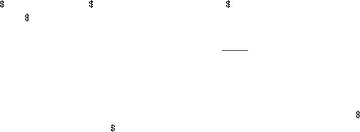
where d
g
is the residual degrees of freedom for the gth gene. Mathematically, 1/˜s
2
g
is derived as the
posterior mean of 1/σ
2
g
conditional on s
2
g
[35, 21]. The output from eBayes() contains s
2
0
and d
0
as
fit s2.prior and fit df.prior and the ˜s
2
j
as fit s2.post. If robust empirical Bayes is used [21],
then fit s2.post is a vector, otherwise it is a single value.
The moderated t-statistic is
˜
t
gk
=
ˆ
β
gk
u
gk
˜s
g
,
which can be shown to follow a t-distribution on d
0
+ d
g
degrees of freedom if β
gk
= 0 [35]. By
comparison, an ordinary t-statistic would have only d
g
degrees of freedom. The prior degrees of
freedom d
0
represent the extra information that is borrowed from the ensemble of genes for inference
about each individual gene. The output from eBayes() contains the
˜
t
gk
as fit t with corresponding
unadjusted p-values in fit p.value.
13.3 Multiple Testing Across Contrasts
The output from topTable includes adjusted p-values, i.e., it performs multiple testing for the contrast
being considered. If several contrasts are being tested simultaneously, then the issue arises of multiple
testing for the entire set of hypotheses being considered, across contrasts as well as probes. The
function decideTests() offers a number of strategies for doing this.
The simplest multiple testing method is method="separate". This method does multiple testing
for each contrast separately. This method is the default because it is equivalent to using topTable().
Using this method, testing a set of contrasts together will give the same results as when each contrast
is tested on its own. The great advantage of this method is that it gives the same results regardless
of which set of contrasts are tested together. The disadvantage of this method is that it does not
do any multiple testing adjustment between contrasts. Another disadvantage is that the raw p-value
cutoff corresponding to significance can be very different for different contrasts, depending on the
number of DE probes. This method is recommended when different contrasts are being analysed to
answer more or less independent questions.
method="global" is recommended when a set of closely related contrasts are being tested. This
method simply appends all the tests together into one long vector of tests, i.e., it treats all the tests
as equivalent regardless of which probe or contrast they relate to. An advantage is that the raw
p-value cutoff is consistent across all contrasts. For this reason, method="global" is recommended if
you want to compare the number of DE genes found for different contrasts, for example interpreting
the number of DE genes as representing the strength of the contrast. However users need to be aware
that the number of DE genes for any particular contrasts will depend on which other contrasts are
tested at the same time. Hence one should include only those contrasts which are closely related to
the question at hand. Unnecessary contrasts should be excluded as these would affect the results for
the contrasts of interest. Another more theoretical issue is that there is no theorem which proves that
adjust.method="BH" in combination with method="global" will correctly control the false discovery
rate for combinations of negatively correlated contrasts, however simulations, experience and some
theory suggest that the method is safe in practice.
The "hierarchical" method offers power advantages when used with adjust.method="holm"
to control the family-wise error rate. However its properties are not yet well understood with
adjust="BH".
method="nestedF" has a more specialized aim to give greater weight to probes that are significance
for two or more contrasts. Most multiple testing methods tend to underestimate the number of such
63
probes. There is some practical experience to suggest that method="nestedF" gives less conservative
results when finding probes which respond to several different contrasts at once. However this method
should still be viewed as experimental. It provides formal false discovery rate control at the probe
level only, not at the contrast level.
64
Chapter 14
Array Quality Weights
14.1 Introduction
Given an appropriate design matrix, the relative reliability of each array in an experiment can be
estimated by measuring how well the expression values for that array follow the linear model. This
empirical approach of assessing array quality can be applied to both two-color and single-channel
microarray data and is described in [25].
The method is implemented in the arrayWeights function, which fits a heteroscedastic model to
the expression values for each gene by calling the function lm.wfit. (See also arrayWeightsSimple
which does the same calculation more quickly when there are no probe-level quality weights.) The
dispersion model is fitted to the squared residuals from the mean fit, and is set up to have array
specific coefficients, which are updated in either full REML scoring iterations, or using an efficient
gene-by-gene update algorithm. The final estimates of these array variances are converted to weights
which can be used in lmFit. This method offers a graduated approach to quality assessment by
allowing poorer quality arrays, which would otherwise be discarded, to be included in an analysis
but down-weighted.
14.2 Example 1
We consider the array quality weights applied to the spike-in controls from a quality control data
set courtesy of Andrew Holloway, Ryan van Laar and Dileepa Diyagama from the Peter MacCallum
Cancer Centre in Melbourne. This collection of arrays (described in [25]) consists of 100 replicate
hybridizations and we will use data from the first 20 arrays. The object MAlms stores the loess
normalized data for the 120 spike-in control probes on each array. Since these arrays are replicate
hybridizations, the default design matrix of a single column of ones is used.
> arrayw <- arrayWeights(MAlms)
> barplot(arrayw, xlab="Array", ylab="Weight", col="white", las=2)
> abline(h=1, lwd=1, lty=2)
65
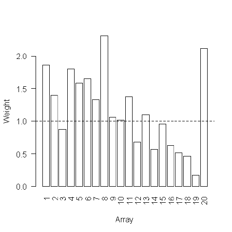
The empirical array weights vary from a minimum of 0.16 for array 19 to a maximum of 2.31 for
array 8. These weights can be used in the linear model analysis.
> fitw <- lmFit(MAlms, weights=arrayw)
> fitw <- eBayes(fitw)
In this example the ratio control spots should show three-fold or ten-fold changes while the
dynamic range spots should not be differentially expressed. To compare the moderated t-statistics
before and after applying array weights, use the following:
> fit <- lmFit(MAlms)
> fit <- eBayes(fit)
> boxplot(fit$t~MAlms$genes$Status, at=1:5-0.2, col=5, boxwex=0.4, xlab="control type",
+ ylab="moderated t-statistics", pch=".", ylim=c(-70, 70), medlwd=1)
> boxplot(fitw$t~MAlms$genes$Status, at=1:5+0.2, col=6, boxwex=0.4,
+ add=TRUE, yaxt="n", xaxt="n", medlwd=1, pch=".")
> abline(h=0, col="black", lty=2, lwd=1)
> legend(0.5, 70, legend=c("Equal weights", "Array weights"), fill=c(5,6), cex=0.8)
66
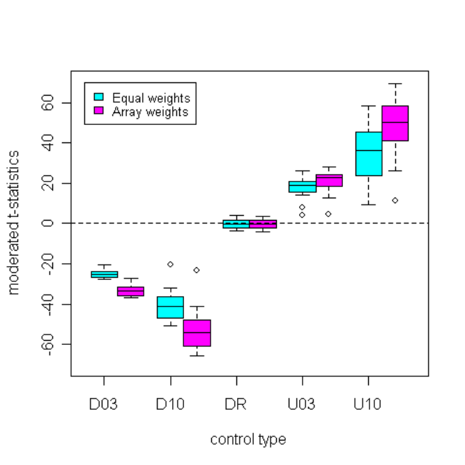
The boxplots show that the t-statistics for all classes of ratio controls (D03, D10, U03 and U10)
move further from zero when array weights are used while the distribution of t-statistics for the
dynamic range controls (DR) does not noticeably change. This demonstrates that the array quality
weights increase statistical power to detect true differential expression without increasing the false
discovery rate.
The same heteroscedastic model can also be fitted at the print-tip group level using the printtipWeights
function. If there are p print-tip groups across n arrays, the model fitting procedure described in [25]
is repeated p times to produce a weight for each print-tip group on each array for use in lmFit. This
method can be applied to two-color microarray data where the probes are organized into print-tip
groups whose size is specified by the printer component of the MAList.
14.3 Example 2
Below is an example of applying this method to the Apoa1 data.
> ptw <- printtipWeights(MA, design, layout=MA$printer)
> zlim <- c(min(ptw), max(ptw))
> par(mfrow=c(3,2))
> for(i in seq(7,12,by=1))
+ imageplot(ptw[,i], layout=MA$printer, zlim=zlim, main=colnames(MA)[i])
67
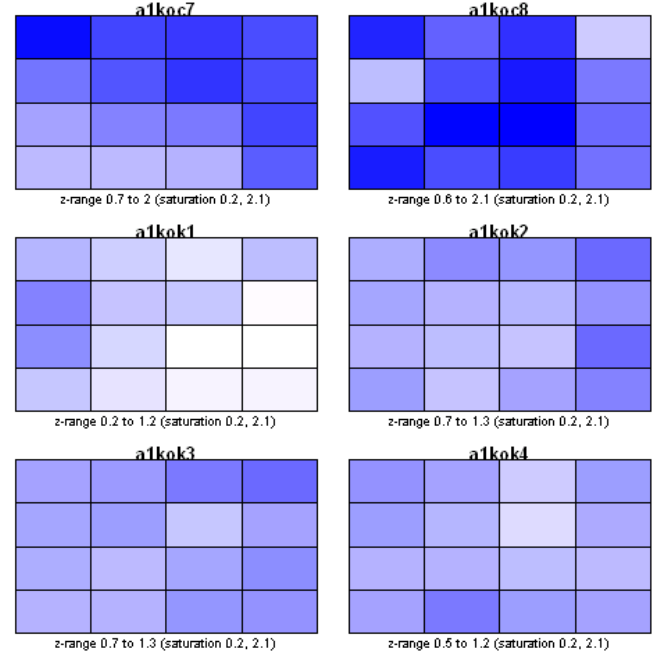
Image plots of the print-tip weights for arrays 7 through to 12 are shown above, with lighter shades
indicating print-tip groups which have been assigned lower weights. A corner of array 9 (a1kok1) is
measured to be less reproducible than the same region on other arrays, which may be indicative of
a spatial artefact. Using these weights in the linear model analysis increases the t-statistics of the
top ranking genes compared to an analysis without weights (compare the results table below with
the table in section 16.2).
> fitptw <- lmFit(MA, design, weights=ptw)
> fitptw <- eBayes(fitptw)
> options(digits=3)
> topTable(fitptw,coef=2,number=15,genelist=fitptw$genes$NAME)
ID logFC AveExpr t P.Value adj.P.Val B
2149 ApoAI,lipid-Img -3.151 12.47 -25.64 1.21e-15 7.73e-12 16.4206
540 EST,HighlysimilartoA -2.918 12.28 -14.49 2.22e-11 7.09e-08 12.4699
5356 CATECHOLO-METHYLTRAN -1.873 12.93 -13.16 1.10e-10 2.34e-07 11.5734
4139 EST,WeaklysimilartoC -0.981 12.61 -11.71 7.28e-10 1.16e-06 10.3623
1739 ApoCIII,lipid-Img -0.933 13.74 -10.58 3.66e-09 4.67e-06 9.4155
1496 est -0.949 12.23 -9.92 9.85e-09 1.05e-05 8.6905
2537 ESTs,Highlysimilarto -1.011 13.63 -9.56 1.75e-08 1.60e-05 8.2587
4941 similartoyeaststerol -0.873 13.29 -6.88 1.93e-06 1.54e-03 4.6875
947 EST,WeaklysimilartoF -0.566 10.54 -5.08 7.78e-05 5.52e-02 1.6112
2812 5’similartoPIR:S5501 -0.514 11.65 -4.30 4.31e-04 2.75e-01 0.1242
6073 estrogenrec 0.412 9.79 4.21 5.27e-04 3.06e-01 -0.0497
1347 Musmusculustranscrip -0.412 10.18 -4.07 7.09e-04 3.47e-01 -0.3106
68
634 MDB1376 -0.380 9.32 -4.07 7.11e-04 3.47e-01 -0.3123
2 Cy5RT 0.673 10.65 4.04 7.61e-04 3.47e-01 -0.3745
5693 Meox2 0.531 9.77 3.84 1.19e-03 4.74e-01 -0.7649
For example, the moderated t-statistic of the top ranked gene, Apoa1, which has been knocked-
out in this experiment, increases in absolute terms from -23.98 when equal weights are used to -25.64
with print-tip weights. The t-statistic of the related gene ApoCIII also increases in absolute value
(moderated t-statistic of -9.83 before weighting and -10.58 after). This analysis provides a further
example that a graduated approach to quality control can improve power to detect differentially
expressed genes.
14.4 When to Use Array Weights
Array weights are generally useful when there is some reason to expect variable array quality. For
example, RNA samples from human clinical patients are typically variable in quality, so array weights
might be used routinely with human in vivo data, see for example Ellis et al [8]. If array quality
plots suggest a problem, then array weights are indicated. If RNA is plentiful, e.g., from cell lines
or model organisms, and quality plots of the arrays don’t suggest problems, then array weights are
usually not needed.
In gross cases where an array is clearly bad or wrong, it should be removed, rather than down-
weighted. However this action should be reserved for extreme cases.
If most genes are not differentially expressed, then the design matrix for arrayWeights does not
need to be as complex as for the final linear model. For example, in a two-group comparison with
just 2 replicates in each group, the array weights should be estimated with the default (intercept)
design matrix, otherwise each array is compared only to its partner rather than to the other 3 arrays.
69
Chapter 15
RNA-Seq Data
15.1 Introduction
The limma approach to RNA-seq explained in the articles by Law et al [13] and Liu et al [17]. See
also the article by Law et al [12], which gives a complete workflow case study. In the limma approach
to RNA-seq, read counts are converted to log2-counts-per-million (logCPM) and the mean-variance
relationship is modeled either with precision weights or with an empirical Bayes prior trend. The
precision weights approach is called “voom” and the prior trend approach is called “limma-trend”
[13]. In either case, the RNA-seq data can be analyzed as if it was microarray data. This means
that any of the linear modeling or gene set testing methods in the limma package can be applied to
RNA-seq data.
15.2 Making a count matrix
RNA-seq data usually arrives in the form of FastQ or BAM files of unaligned reads. The reads need
to be mapped to a reference genome or transcriptome, then summarized at the exon or gene level to
produce a matrix of counts. We find the Rsubread package [15] to be convenient, fast and effective
for this purpose. Other popular methods include RSEM [14] and HTseq. A runnable example
with complete code showing how to use Rsubread with limma is provided at https://subread.
sourceforge.net/RNAseqCaseStudy.html. Another complete code example is provided by Chen et
al [5].
15.3 Normalization and filtering
Once a matrix of read counts counts has been created, with rows for genes and columns for samples,
it is convenient to create a DGEList object using the edgeR package:
> dge <- DGEList(counts=counts)
The next step is to remove rows that consistently have zero or very low counts. One can for
example use
> keep <- filterByExpr(dge, design)
> dge <- dge[keep,,keep.lib.sizes=FALSE]
70
where filterByExpr is a function in the edgeR package. Here we will assume that filtering has been
done.
It is usual to apply scale normalization to RNA-seq read counts, and the TMM normalization
method [28] in particular has been found to perform well in comparative studies. This can be applied
to the DGEList object:
> dge <- calcNormFactors(dge)
15.4 Differential expression: limma-trend
If the sequencing depth is reasonably consistent across the RNA samples, then the simplest and most
robust approach to differential exis to use limma-trend. This approach will usually work well if the
ratio of the largest library size to the smallest is not more than about 3-fold.
In the limma-trend approach, the counts are converted to logCPM values using edgeR’s cpm
function:
> logCPM <- cpm(dge, log=TRUE, prior.count=3)
The prior count is used here to damp down the variances of logarithms of low counts.
The logCPM values can then be used in any standard limma pipeline, using the trend=TRUE
argument when running eBayes or treat. For example:
> fit <- lmFit(logCPM, design)
> fit <- eBayes(fit, trend=TRUE)
> topTable(fit, coef=ncol(design))
Or, to give more weight to fold-changes in the gene ranking, one might use:
> fit <- lmFit(logCPM, design)
> fit <- treat(fit, lfc=log2(1.2), trend=TRUE)
> topTreat(fit, coef=ncol(design))
15.5 Differential expression: voom
When the library sizes are quite variable between samples, then the voom approach is theoretically
more powerful than limma-trend. In this approach, the voom transformation is applied to the
normalized and filtered DGEList object:
v <- voom(dge, design, plot=TRUE)
The voom transformation uses the experiment design matrix, and produces an EList object.
It is also possible to give a matrix of counts directly to voom without TMM normalization, by
> v <- voom(counts, design, plot=TRUE)
If the data are very noisy, one can apply the same between-array normalization methods as would
be used for microarrays, for example:
> v <- voom(counts, design, plot=TRUE, normalize="quantile")
After this, the usual limma pipelines for differential expression can be applied, for example:
71
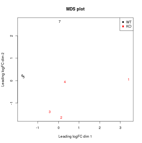
> fit <- lmFit(v, design)
> fit <- eBayes(fit)
> topTable(fit, coef=ncol(design))
Or, to give more weight to fold-changes in the ranking, one could use say:
> fit <- treat(fit, lfc=log2(1.2))
> topTreat(fit, coef=ncol(design))
15.6 Voom with sample quality weights
When a multi-dimensional scaling plot from a designed RNA-seq experiment indicates the presence
of outlier samples, it is possible to combine the observation-level weighting strategy used in voom
with sample-specific quality weights (as described in the section above on Array Quality Weights) to
down-weight outlier samples. This capability is implemented in the voomWithQualityWeights function.
The example below shows its use on an RNA-seq data set where the epigenetic regulator Smchd1
has been knocked-out in lymphoma cell-lines (GEO series GSE64099) [17]. Overall we obtain more
differential expression by applying this combined weighting strategy and the raw p-value and false
discovery rate for the Smchd1 gene, which has been knocked out, is smaller.
> plotMDS(x, labels=1:7, col=as.numeric(genotype), main="MDS plot")
> legend("topright", legend=c("WT", "KO"), col=1:2, pch=15)
> # Analysis with voom only
> des[1:7,]
(Intercept) Smchd1nullvsWt
1 1 1
2 1 1
3 1 1
4 1 1
5 1 0
72
6 1 0
7 1 0
> v <- voom(x, design=des)
> plotMDS(v, labels=1:7, col=as.numeric(genotype))
> vfit <- lmFit(v)
> vfit <- eBayes(vfit)
> options(digits=3)
> topTable(vfit,coef=2,sort.by="P")
GeneID Symbols logFC AveExpr t P.Value adj.P.Val B
74355 74355 Smchd1 -3.12 6.067 -23.35 2.16e-08 0.000266 9.97
18028 18028 Nfib 8.98 1.714 12.60 2.17e-06 0.013355 3.15
75605 75605 Kdm5b -3.55 3.618 -11.75 3.62e-06 0.014857 5.06
667435 667435 Igkv17-121 -5.35 -1.435 -10.22 9.95e-06 0.025513 2.57
381126 381126 Garem 6.17 0.113 10.08 1.10e-05 0.025513 2.35
381413 381413 Gpr176 -4.02 1.328 -9.90 1.25e-05 0.025513 3.39
75033 75033 Mei4 6.44 0.259 9.69 1.45e-05 0.025513 2.23
69136 69136 Tusc1 5.67 -0.184 8.90 2.67e-05 0.040995 1.87
233552 233552 Gdpd5 -2.82 1.948 -8.56 3.49e-05 0.042754 2.81
80890 80890 Trim2 -1.43 4.491 -8.40 4.00e-05 0.042754 2.72
> top <- topTable(vfit,coef=2,number=Inf,sort.by="P")
> sum(top$adj.P.Val<0.05)
[1] 12
> # Analysis with combined voom and sample quality weights
> vwts <- voomWithQualityWeights(x, design=des, normalization="none", plot=TRUE)
> vfit2 <- lmFit(vwts)
> vfit2 <- eBayes(vfit2)
> topTable(vfit2,coef=2,sort.by="P")
GeneID Symbols logFC AveExpr t P.Value adj.P.Val B
74355 74355 Smchd1 -3.17 6.067 -28.5 1.61e-09 1.98e-05 12.57
18028 18028 Nfib 9.23 1.714 19.0 4.44e-08 2.73e-04 6.91
381126 381126 Garem 6.45 0.113 15.9 1.85e-07 7.58e-04 6.02
75033 75033 Mei4 6.56 0.259 15.0 2.84e-07 8.73e-04 5.83
69136 69136 Tusc1 5.88 -0.184 13.6 6.16e-07 1.11e-03 5.31
54354 54354 Rassf5 5.74 4.554 13.6 6.26e-07 1.11e-03 6.63
75605 75605 Kdm5b -3.80 3.618 -13.5 6.53e-07 1.11e-03 6.67
58998 58998 Pvrl3 7.69 0.961 13.1 8.46e-07 1.11e-03 5.33
320398 320398 Lrig3 7.39 1.584 13.1 8.49e-07 1.11e-03 5.32
17069 17069 Ly6e 2.63 7.605 13.0 9.01e-07 1.11e-03 6.26
> top2 <- topTable(vfit2,coef=2,number=Inf,sort.by="P")
> sum(top2$adj.P.Val<0.05)
[1] 1478
73
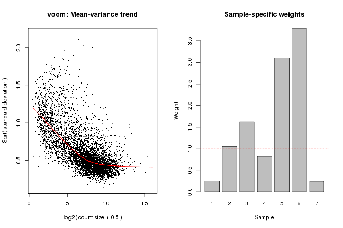
15.7 Differential splicing
limma can also detect genes that how evidence of differential splicing between conditions. One can
test for differential splicing associated with any contrast for a linear model.
In this case, the matrix of counts should be at the exon level, with a row for each exon. For
example,
> dge <- DGEList(counts=counts)
> dge$genes$GeneID <- GeneID
where counts is a matrix of exon-level counts, and GeneID identifies which gene each exon belongs
to. Then filter and normalize:
> A <- rowSums(dge$counts)
> dge <- dge[A>10,, keep.lib.sizes=FALSE]
> dge <- calcNormFactors(dge)
Then apply the voom transformation and fit a linear model:
> v <- voom(dge, design, plot=TRUE)
> fit <- lmFit(v, design)
Now we can test for differential splicing associated with any coefficient in the linear model. First
run the diffSplice function:
> ex <- diffSplice(fit, geneid="GeneID")
Then
> topSplice(ex, coef=2, test="simes")
will find genes that show evidence of differential splicing associated with the second coefficient in
the linear model. The output is similar that from the limma topTable function. More detail can be
obtained by
74
> topSplice(ex, coef=2, test="t")
which will show individual exons that are enriched or depleted relative to other exons in the same
gene. To display the pattern of exons in the top genes:
> plotSplice(ex)
75
Chapter 16
Two-Color Case Studies
16.1 Swirl Zebrafish: A Single-Group Experiment
In this section we consider a case study in which two RNA sources are compared directly on a
set of replicate or dye-swap arrays. The case study includes reading in the data, data display and
exploration, as well as normalization and differential expression analysis. The analysis of differential
expression is analogous to a classical one-sample test of location for each gene.
In this example we assume that the data is provided as a GAL file called fish.gal and raw SPOT
output files and that these files are in the current working directory. The data used for this case
study can be downloaded from https://bioinf.wehi.edu.au/limmaGUI/DataSets.html.
> dir()
[1] "fish.gal" "swirl.1.spot" "swirl.2.spot" "swirl.3.spot" "swirl.4.spot"
[6] "SwirlSample.txt"
Background. The experiment was carried out using zebrafish as a model organism to study the early
development in vertebrates. Swirl is a point mutant in the BMP2 gene that affects the dorsal/ventral
body axis. The main goal of the Swirl experiment is to identify genes with altered expression in the
Swirl mutant compared to wild-type zebrafish.
The hybridizations. Two sets of dye-swap experiments were performed making a total of four repli-
cate hybridizations. Each of the arrays compares RNA from swirl fish with RNA from normal (“wild
type”) fish. The experimenters have prepared a tab-delimited targets file called SwirlSamples.txt
which describes the four hybridizations:
> library(limma)
> targets <- readTargets("SwirlSample.txt")
> targets
SlideNumber FileName Cy3 Cy5 Date
1 81 swirl.1.spot swirl wild type 2001/9/20
2 82 swirl.2.spot wild type swirl 2001/9/20
3 93 swirl.3.spot swirl wild type 2001/11/8
4 94 swirl.4.spot wild type swirl 2001/11/8
We see that slide numbers 81, 82, 93 and 94 were used to make the arrays. On slides 81 and 93,
swirl RNA was labeled with green (Cy3) dye and wild type RNA was labeled with red (Cy5) dye.
On slides 82 and 94, the labelling was the other way around.
76
Each of the four hybridized arrays was scanned on an Axon scanner to produce a TIFF image,
which was then processed using the image analysis software SPOT. The data from the arrays are
stored in the four output files listed under FileName. Now we read the intensity data into an RGList
object in R. The default for SPOT output is that Rmean and Gmean are used as foreground intensities
and morphR and morphG are used as background intensities:
> RG <- read.maimages(targets, source="spot")
Read swirl.1.spot
Read swirl.2.spot
Read swirl.3.spot
Read swirl.4.spot
> RG
An object of class "RGList"
$R
swirl.1 swirl.2 swirl.3 swirl.4
[1,] 19538.470 16138.720 2895.1600 14054.5400
[2,] 23619.820 17247.670 2976.6230 20112.2600
[3,] 21579.950 17317.150 2735.6190 12945.8500
[4,] 8905.143 6794.381 318.9524 524.0476
[5,] 8676.095 6043.542 780.6667 304.6190
8443 more rows ...
$G
swirl.1 swirl.2 swirl.3 swirl.4
[1,] 22028.260 19278.770 2727.5600 19930.6500
[2,] 25613.200 21438.960 2787.0330 25426.5800
[3,] 22652.390 20386.470 2419.8810 16225.9500
[4,] 8929.286 6677.619 383.2381 786.9048
[5,] 8746.476 6576.292 901.0000 468.0476
8443 more rows ...
$Rb
swirl.1 swirl.2 swirl.3 swirl.4
[1,] 174 136 82 48
[2,] 174 133 82 48
[3,] 174 133 76 48
[4,] 163 105 61 48
[5,] 140 105 61 49
8443 more rows ...
$Gb
swirl.1 swirl.2 swirl.3 swirl.4
[1,] 182 175 86 97
[2,] 171 183 86 85
[3,] 153 183 86 85
[4,] 153 142 71 87
[5,] 153 142 71 87
8443 more rows ...
$targets
SlideNumber FileName Cy3 Cy5 Date
1 81 swirl.1.spot swirl wild type 2001/9/20
2 82 swirl.2.spot wild type swirl 2001/9/20
3 93 swirl.3.spot swirl wild type 2001/11/8
4 94 swirl.4.spot wild type swirl 2001/11/8
77
$source
[1] "spot"
The arrays. The microarrays used in this experiment were printed with 8448 probes (spots),
including 768 control spots. The array printer uses a print head with a 4x4 arrangement of print-tips
and so the microarrays are partitioned into a 4x4 grid of tip groups. Each grid consists of 22x24
spots that were printed with a single print-tip.
Unlike most image analysis software, SPOT does not store probe annotation in the output files,
so we have to read it separately. The gene name associated with each spot is recorded in a GenePix
array list (GAL) file:
> RG$genes <- readGAL("fish.gal")
> RG$genes[1:30,]
Block Row Column ID Name
1 1 1 1 control geno1
2 1 1 2 control geno2
3 1 1 3 control geno3
4 1 1 4 control 3XSSC
5 1 1 5 control 3XSSC
6 1 1 6 control EST1
7 1 1 7 control geno1
8 1 1 8 control geno2
9 1 1 9 control geno3
10 1 1 10 control 3XSSC
11 1 1 11 control 3XSSC
12 1 1 12 control 3XSSC
13 1 1 13 control EST2
14 1 1 14 control EST3
15 1 1 15 control EST4
16 1 1 16 control 3XSSC
17 1 1 17 control Actin
18 1 1 18 control Actin
19 1 1 19 control 3XSSC
20 1 1 20 control 3XSSC
21 1 1 21 control 3XSSC
22 1 1 22 control 3XSSC
23 1 1 23 control Actin
24 1 1 24 control Actin
25 1 2 1 control ath1
26 1 2 2 control Cad-1
27 1 2 3 control DeltaB
28 1 2 4 control Dlx4
29 1 2 5 control ephrinA4
30 1 2 6 control FGF8
Because we are using SPOT output, the 4x4x22x24 print layout also needs to be set. The easiest
way to do this is to infer it from the GAL file:
> RG$printer <- getLayout(RG$genes)
Image plots. It is interesting to look at the variation of background values over the array. Consider
image plots of the red and green background for the first array:
78
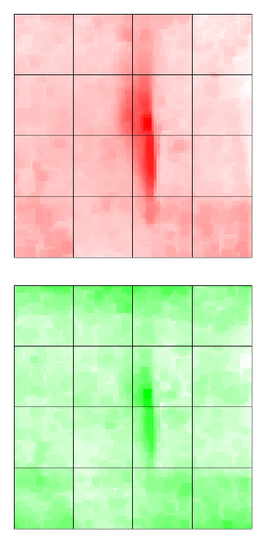
> imageplot(log2(RG$Rb[,1]), RG$printer, low="white", high="red")
> imageplot(log2(RG$Gb[,1]), RG$printer, low="white", high="green")
Image plot of the un-normalized log-ratios or M-values for the first array:
> MA <- normalizeWithinArrays(RG, method="none")
> imageplot(MA$M[,1], RG$printer, zlim=c(-3,3))
79
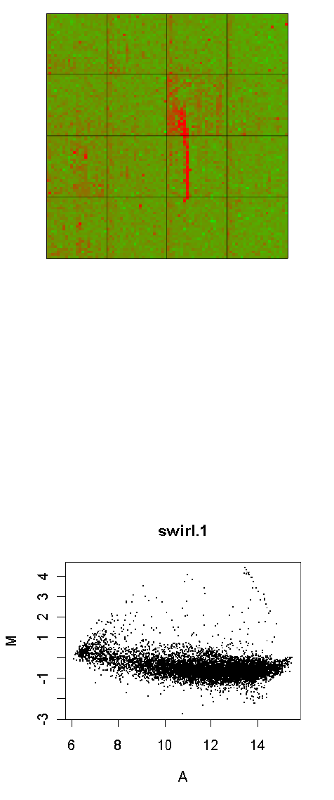
The imageplot function lies the slide on its side, so the first print-tip group is bottom left in this
plot. We can see a red streak across the middle two grids of the 3rd row caused by a scratch or dust
on the array. Spots which are affected by this artifact will have suspect M-values. The streak also
shows up as darker regions in the background plots.
MA-plots. An MA-plot plots the log-ratio of R vs G against the overall intensity of each spot. The
log-ratio is represented by the M-value, M = log
2
(R) − log
2
(G), and the overall intensity by the
A-value, A = (log
2
(R) + log
2
(G))/2. Here is the MA-plot of the un-normalized values for the first
array:
> plotMD(MA)
The red streak seen on the image plot can be seen as a line of spots in the upper right of this plot.
Now we plot the individual MA-plots for each of the print-tip groups on this array, together with
the loess curves which will be used for normalization:
80
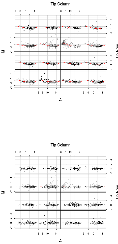
> plotPrintTipLoess(MA)
Normalization. Print-tip loess normalization:
> MA <- normalizeWithinArrays(RG)
> plotPrintTipLoess(MA)
We have normalized the M-values with each array. A further question is whether normalization is
required between the arrays. The following plot shows overall boxplots of the M-values for the four
arrays.
> boxplot(MA$M~col(MA$M),names=colnames(MA$M))
81
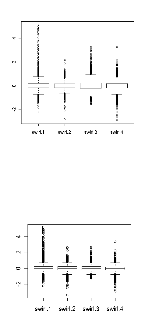
There is evidence that the different arrays have different spreads of M-values, so we will scale
normalize between the arrays.
> MA <- normalizeBetweenArrays(MA,method="scale")
> boxplot(MA$M~col(MA$M),names=colnames(MA$M))
Note that scale-normalization is not done routinely for all two-color data sets, in fact it is rarely
done with newer platforms. However it does give good results on this data set. It should only be
done when there is good evidence of a scale difference in the M-values.
Linear model. First setup an appropriate design matrix. The negative numbers in the design
matrix indicate the dye-swaps:
82
> design <- modelMatrix(targets, ref="wild type")
Found unique target names:
swirl wild type
> design
swirl
swirl.1 -1
swirl.2 1
swirl.3 -1
swirl.4 1
Now fit a simple linear model for each gene. This has the effect of estimating the average M-value
for each gene, adjusting for the dye-swaps.
> fit <- lmFit(MA,design)
> fit
An object of class "MArrayLM"
$coefficients
[1] -0.3556298 -0.3283455 -0.3455845 -0.2254783 -0.3175470
8443 more rows ...
$rank
[1] 1
$assign
NULL
$qr
$qr
[,1]
[1,] 2.0
[2,] -0.5
[3,] 0.5
[4,] -0.5
$qraux
[1] 1.5
$pivot
[1] 1
$tol
[1] 1e-07
$rank
[1] 1
$df.residual
[1] 3 3 3 3 3
8443 more elements ...
$sigma
[1] 0.2873571 0.3115307 0.3699258 0.3331054 0.2689609
8443 more elements ...
$cov.coefficients
[,1]
83
[1,] 0.25
$stdev.unscaled
[1] 0.5 0.5 0.5 0.5 0.5
8443 more rows ...
$pivot
[1] 1
$genes
Block Row Column ID Name
1 1 1 1 control geno1
2 1 1 2 control geno2
3 1 1 3 control geno3
4 1 1 4 control 3XSSC
5 1 1 5 control 3XSSC
8443 more rows ...
$Amean
[1] 13.44500 13.65700 13.40297 10.71737 10.83383
8443 more elements ...
$method
[1] "ls"
$design
[,1]
[1,] -1
[2,] 1
[3,] -1
[4,] 1
In the above fit object, coefficients is the average M-value for each gene and sigma is the sam-
ple standard deviations for each gene. Ordinary t-statistics for comparing mutant to wt could be
computed by
> ordinary.t <- fit$coef / fit$stdev.unscaled / fit$sigma
We prefer though to use empirical Bayes moderated t-statistics which are computed below.
Now create an mean difference plot displaying the log-fold-changes and average A-values for each
gene.
> plotMD(fit)
> abline(0,0,col="blue")
84
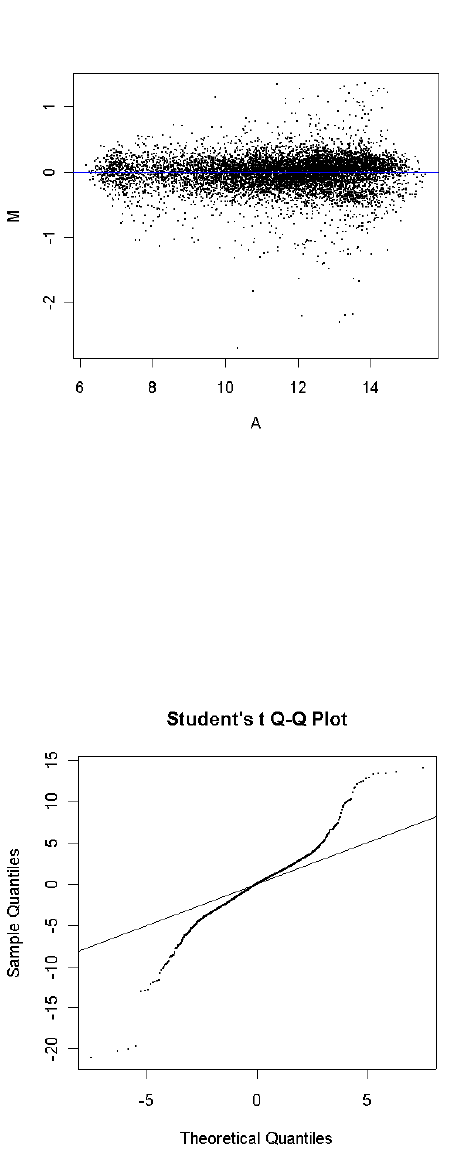
Empirical Bayes analysis. We will now go on and compute empirical Bayes statistics for differen-
tial expression. The moderated t-statistics use sample standard deviations which have been squeezed
towards a pooled standard deviation value.
> fit <- eBayes(fit)
> qqt(fit$t,df=fit$df.prior+fit$df.residual,pch=16,cex=0.2)
> abline(0,1)
Visually there seems to be plenty of genes which are differentially expressed. We will obtain a
summary table of some key statistics for the top genes.
85
> options(digits=3)
> topTable(fit,number=30)
Block Row Column ID Name logFC AveExpr t P.Value adj.P.Val B
3721 8 2 1 control BMP2 -2.21 12.1 -21.1 1.03e-07 0.000357 7.96
1609 4 2 1 control BMP2 -2.30 13.1 -20.3 1.34e-07 0.000357 7.78
3723 8 2 3 control Dlx3 -2.18 13.3 -20.0 1.48e-07 0.000357 7.71
1611 4 2 3 control Dlx3 -2.18 13.5 -19.6 1.69e-07 0.000357 7.62
8295 16 16 15 fb94h06 20-L12 1.27 12.0 14.1 1.74e-06 0.002067 5.78
7036 14 8 4 fb40h07 7-D14 1.35 13.8 13.5 2.29e-06 0.002067 5.54
515 1 22 11 fc22a09 27-E17 1.27 13.2 13.4 2.44e-06 0.002067 5.48
5075 10 14 11 fb85f09 18-G18 1.28 14.4 13.4 2.46e-06 0.002067 5.48
7307 14 19 11 fc10h09 24-H18 1.20 13.4 13.2 2.67e-06 0.002067 5.40
319 1 14 7 fb85a01 18-E1 -1.29 12.5 -13.1 2.91e-06 0.002067 5.32
2961 6 14 9 fb85d05 18-F10 -2.69 10.3 -13.0 3.04e-06 0.002067 5.29
4032 8 14 24 fb87d12 18-N24 1.27 14.2 12.8 3.28e-06 0.002067 5.22
6903 14 2 15 control Vox -1.26 13.4 -12.8 3.35e-06 0.002067 5.20
4546 9 14 10 fb85e07 18-G13 1.23 14.2 12.8 3.42e-06 0.002067 5.18
683 2 7 11 fb37b09 6-E18 1.31 13.3 12.4 4.10e-06 0.002182 5.02
1697 4 5 17 fb26b10 3-I20 1.09 13.3 12.4 4.30e-06 0.002182 4.97
7491 15 5 3 fb24g06 3-D11 1.33 13.6 12.3 4.39e-06 0.002182 4.96
4188 8 21 12 fc18d12 26-F24 -1.25 12.1 -12.2 4.71e-06 0.002209 4.89
4380 9 7 12 fb37e11 6-G21 1.23 14.0 12.0 5.19e-06 0.002216 4.80
3726 8 2 6 control fli-1 -1.32 10.3 -11.9 5.40e-06 0.002216 4.76
2679 6 2 15 control Vox -1.25 13.4 -11.9 5.72e-06 0.002216 4.71
5931 12 6 3 fb32f06 5-C12 -1.10 13.0 -11.7 6.24e-06 0.002216 4.63
7602 15 9 18 fb50g12 9-L23 1.16 14.0 11.7 6.25e-06 0.002216 4.63
2151 5 2 15 control vent -1.40 12.7 -11.7 6.30e-06 0.002216 4.62
3790 8 4 22 fb23d08 2-N16 1.16 12.5 11.6 6.57e-06 0.002221 4.58
7542 15 7 6 fb36g12 6-D23 1.12 13.5 11.0 9.23e-06 0.003000 4.27
4263 9 2 15 control vent -1.41 12.7 -10.8 1.06e-05 0.003326 4.13
6375 13 2 15 control vent -1.37 12.5 -10.5 1.33e-05 0.004026 3.91
1146 3 4 18 fb22a12 2-I23 1.05 13.7 10.2 1.57e-05 0.004242 3.76
157 1 7 13 fb38a01 6-I1 -1.82 10.8 -10.2 1.58e-05 0.004242 3.75
The top gene is BMP2 which is significantly down-regulated in the Swirl zebrafish, as it should be
because the Swirl fish are mutant in this gene. Other positive controls also appear in the top 30
genes in terms.
In the table, t is the empirical Bayes moderated t-statistic, the corresponding P-values have
been adjusted to control the false discovery rate and B is the empirical Bayes log odds of differential
expression.
> plotMD(fit)
> top30 <- order(fit$lods,decreasing=TRUE)[1:30]
> text(fit$Amean[top30],fit$coef[top30],labels=fit$genes[top30,"Name"],cex=0.8,col="blue")
86
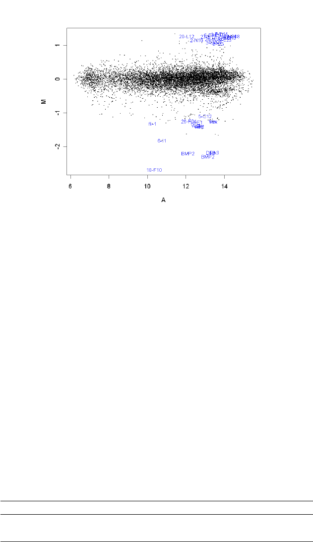
16.2 Apoa1 Knockout Mice: A Two-Group Common-Reference
Experiment
In this section we consider a case study where two RNA sources are compared through a common
reference RNA. The analysis of the log-ratios involves a two-sample comparison of means for each
gene.
In this example we assume that the data is available as an RGList in the data file Apoa1.RData.
The data used for this case study can be downloaded from https://bioinf.wehi.edu.au/limma.
Background. The data is from a study of lipid metabolism by [3]. The apolipoprotein AI (Apoa1)
gene is known to play a pivotal role in high density lipoprotein (HDL) metabolism. Mice which have
the Apoa1 gene knocked out have very low HDL cholesterol levels. The purpose of this experiment
is to determine how Apoa1 deficiency affects the action of other genes in the liver, with the idea that
this will help determine the molecular pathways through which Apoa1 operates.
Hybridizations. The experiment compared 8 Apoa1 knockout mice with 8 normal C57BL/6 (”black
six”) mice, the control mice. For each of these 16 mice, target mRNA was obtained from liver tissue
and labelled using a Cy5 dye. The RNA from each mouse was hybridized to a separate microarray.
Common reference RNA was labelled with Cy3 dye and used for all the arrays. The reference RNA
was obtained by pooling RNA extracted from the 8 control mice.
Number of arrays Red Green
8 Normal “black six” mice Pooled reference
8 Apoa1 knockout Pooled reference
This is an example of a single comparison experiment using a common reference. The fact that the
comparison is made by way of a common reference rather than directly as for the swirl experiment
makes this, for each gene, a two-sample rather than a single-sample setup.
> load("Apoa1.RData")
> objects()
87
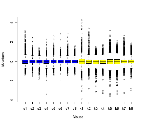
[1] "RG"
> names(RG)
[1] "R" "G" "Rb" "Gb" "printer" "genes" "targets"
> RG$targets
FileName Cy3 Cy5
c1 a1koc1.spot Pool C57BL/6
c2 a1koc2.spot Pool C57BL/6
c3 a1koc3.spot Pool C57BL/6
c4 a1koc4.spot Pool C57BL/6
c5 a1koc5.spot Pool C57BL/6
c6 a1koc6.spot Pool C57BL/6
c7 a1koc7.spot Pool C57BL/6
c8 a1koc8.spot Pool C57BL/6
k1 a1kok1.spot Pool ApoAI-/-
k2 a1kok2.spot Pool ApoAI-/-
k3 a1kok3.spot Pool ApoAI-/-
k4 a1kok4.spot Pool ApoAI-/-
k5 a1kok5.spot Pool ApoAI-/-
k6 a1kok6.spot Pool ApoAI-/-
k7 a1kok7.spot Pool ApoAI-/-
k8 a1kok8.spot Pool ApoAI-/-
> MA <- normalizeWithinArrays(RG)
> cols <- MA$targets$Cy5
> cols[cols=="C57BL/6"] <- "blue"
> cols[cols=="ApoAI-/-"] <- "yellow"
> boxplot(MA$M~col(MA$M),names=rownames(MA$targets),col=cols,xlab="Mouse",ylab="M-values")
Since the common reference here is a pool of the control mice, we expect to see more differences from
the pool for the knock-out mice than for the control mice. In terms of the above plot, this should
translate into a wider range of M-values for the knock-out mice arrays than for the control arrays,
and we do see this. Since the different arrays are not expected to have the same range of M-values,
between-array scale normalization of the M-values is not appropriate here.
Now we can go on to estimate the fold change between the two groups. In this case the design
matrix has two columns. The coefficient for the second column estimates the parameter of interest,
the log-ratio between knockout and control mice.
88
> design <- cbind("Control-Ref"=1,"KO-Control"=MA$targets$Cy5=="ApoAI-/-")
> design
Control-Ref KO-Control
[1,] 1 0
[2,] 1 0
[3,] 1 0
[4,] 1 0
[5,] 1 0
[6,] 1 0
[7,] 1 0
[8,] 1 0
[9,] 1 1
[10,] 1 1
[11,] 1 1
[12,] 1 1
[13,] 1 1
[14,] 1 1
[15,] 1 1
[16,] 1 1
> fit <- lmFit(MA, design)
> fit$coef[1:5,]
Control-Ref KO-Control
[1,] -0.6595 0.6393
[2,] 0.2294 0.6552
[3,] -0.2518 0.3342
[4,] -0.0517 0.0405
[5,] -0.2501 0.2230
> fit <- eBayes(fit)
> options(digits=3)
Normally at this point one would just type
> topTable(fit,coef=2)
However, the gene annotation is a bit wide for the printed page, so we will tell topTable() to show
just one column of the annotation information:
> topTable(fit,coef=2,number=15,genelist=fit$genes$NAME)
ID logFC AveExpr t P.Value adj.P.Val B
2149 ApoAI,lipid-Img -3.166 12.47 -23.98 4.77e-15 3.05e-11 14.927
540 EST,HighlysimilartoA -3.049 12.28 -12.96 1.57e-10 5.02e-07 10.813
5356 CATECHOLO-METHYLTRAN -1.848 12.93 -12.44 3.06e-10 6.51e-07 10.448
4139 EST,WeaklysimilartoC -1.027 12.61 -11.76 7.58e-10 1.21e-06 9.929
1739 ApoCIII,lipid-Img -0.933 13.74 -9.84 1.22e-08 1.56e-05 8.192
2537 ESTs,Highlysimilarto -1.010 13.63 -9.02 4.53e-08 4.22e-05 7.305
1496 est -0.977 12.23 -9.00 4.63e-08 4.22e-05 7.290
4941 similartoyeaststerol -0.955 13.29 -7.44 7.04e-07 5.62e-04 5.311
947 EST,WeaklysimilartoF -0.571 10.54 -4.55 2.49e-04 1.77e-01 0.563
5604 -0.366 12.71 -3.96 9.22e-04 5.29e-01 -0.553
4140 APXL2,5q-Img -0.420 9.79 -3.93 9.96e-04 5.29e-01 -0.619
6073 estrogenrec 0.421 9.79 3.91 1.03e-03 5.29e-01 -0.652
1337 psoriasis-associated -0.838 11.66 -3.89 1.08e-03 5.29e-01 -0.687
954 Caspase7,heart-Img -0.302 12.14 -3.86 1.17e-03 5.30e-01 -0.757
563 FATTYACID-BINDINGPRO -0.637 11.62 -3.81 1.29e-03 5.30e-01 -0.839
Notice that the top gene is Apoa1 itself which is heavily down-regulated. Theoretically the M-value
should be minus infinity for Apoa1 because it is the knockout gene. Several of the other genes are
89
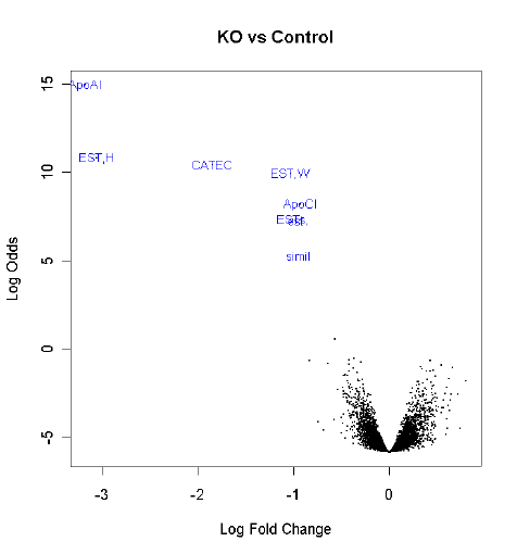
closely related. The top eight genes here were confirmed by independent assay subsequent to the
microarray experiment to be differentially expressed in the knockout versus the control line.
> volcanoplot(fit,coef=2,highlight=8,names=fit$genes$NAME,main="KO vs Control")
16.3 Weaver Mutant Mice: A Composite 2x2 Factorial Experiment
16.3.1 Background
This case study considers a more involved two-color analysis in which the RNA sources have a
factorial structure with two factors.
The study examined the development of neurons in wild-type and weaver mutant mice [7]. The
weaver mutation affects cerebellar granule neurons, the most numerous cell-type in the central ner-
vous system. Weaver mutant mice are characterized by a weaving gait. Granule cells are generated
in the first postnatal week in the external granule layer of the cerebellum. In normal mice, the
terminally differentiated granule cells migrate to the internal granule layer but in mutant mice the
cells die before doing so, meaning that the mutant mice have strongly reduced numbers of cells in
the internal granule layer. The expression level of any gene which is specific to mature granule cells,
or is expressed in response to granule cell derived signals, is greatly reduced in the mutant mice.
16.3.2 Sample Preparation and Hybridizations
At each time point (P11 = 11 days postnatal and P21 = 21 days postnatal) cerebella were isolated
from two wild-type and two mutant littermates and pooled for RNA isolation. RNA was then divided
into aliquots and labelled before hybridizing to the arrays. (This means that aliquots are technical
replicates, arising from the same mice and RNA extraction. In our analysis here, we will ignore this
complication and will instead treat the aliquots as if they were biological replicates. See Yang and
90
Speed (2002) for a detailed discussion of this issue in the context of this experiment.) A pool of RNA
was also made by combining the different RNA samples.
There are four different treatment combinations, P11wt, P11mt, P21wt and P21mt, comprising
a 2x2 factorial structure. The RNA samples were hybridized to ten two-color microarrays, spotted
with a 20k Riken clone library. There are six arrays comparing the four different RNA sources to the
RNA pool, and four arrays making direct comparisons between the four treatment combinations.
The microarray images were scanned using SPOT image analysis software.
16.3.3 Data input
The data used for this case study can be downloaded from http://bioinf.wehi.edu.au/limma/
data/weaverfull.rar. The data are provided courtesy of Drs Jean Yang and Elva Diaz.
First read in the targets frame:
> library(limma)
> targets <- readTargets("targets.txt")
> rownames(targets) <- removeExt(targets$FileName)
> targets
FileName Tissue Mouse Cy5 Cy3
cbmut.3 cbmut.3.spot Cerebellum Weaver P11wt Pool
cbmut.4 cbmut.4.spot Cerebellum Weaver P11mt Pool
cbmut.5 cbmut.5.spot Cerebellum Weaver P21mt Pool
cbmut.6 cbmut.6.spot Cerebellum Weaver P21wt Pool
cbmut.15 cbmut.15.spot Cerebellum Weaver P21wt Pool
cbmut.16 cbmut.16.spot Cerebellum Weaver P21mt Pool
cb.1 cb.1.spot Cerebellum Weaver P11wt P11mt
cb.2 cb.2.spot Cerebellum Weaver P11mt P21mt
cb.3 cb.3.spot Cerebellum Weaver P21mt P21wt
cb.4 cb.4.spot Cerebellum Weaver P21wt P11wt
Exploratory analysis showed that the segmented area for spots for these arrays was quite variable,
with a median spot area just over 50 pixels. A small proportion of spots had very small segmented
sizes, suggesting that the intensities for these spots might be unreliable. It was therefore decided
to set a spot quality weight function, so any spot with an area less than 50 pixels will get reduced
weight. The function is set so that any spot with zero area will get zero weight:
> wtfun <- function(x) pmin(x$area/50, 1)
Then read the SPOT files containing the intensity data using file names recorded in the targets
file. The data files are stored in the subdirectory /spot:
> RG <- read.maimages(targets, source = "spot", path = "spot", wt.fun = wtfun)
Read spot/cbmut.3.spot
Read spot/cbmut.4.spot
Read spot/cbmut.5.spot
Read spot/cbmut.6.spot
Read spot/cbmut.15.spot
Read spot/cbmut.16.spot
Read spot/cb.1.spot
Read spot/cb.2.spot
Read spot/cb.3.spot
Read spot/cb.4.spot
Finally, we set the print-tip layout. These arrays were printed using a print-head with 8 rows
and 4 columns of print tips:
> RG$printer <- list(ngrid.r = 8, ngrid.c = 4, nspot.r = 25, nspot.c = 24)
91
16.3.4 Annotation
Probe annotation is contained a separate file. The rows in the annotation file are as for the intensity
data. Columns give Riken chip rearray IDs, GenBank accession numbers and UniGene information.
> Annotation <- read.delim("091701RikenUpdatev3.txt", comment.char="", quote="\"",
+ check.names=FALSE, stringsAsFactors=FALSE)
> names(Annotation)
[1] "ReArrayID" "Accession #, GenBank" "description (Riken)"
[4] "Cluster ID (UniGene)" "2nd description (UniGene)"
For our purposes, we will keep the Riken IDs and GenBank accessions, putting these into the data
object:
> RG$genes <- Annotation[,c(1,2)]
> colnames(RG$genes) <- c("RikenID","GenBank")
Where possible, we find gene symbols corresponding to the GenBank accession numbers, by using
the mouse organism package constructed from the NCBI database. Symbols can be found for only a
little over 5000 of the probes.
> library(org.Mm.eg.db)
First we find the Entrez Gene ID for each accession number:
> EG.AN <- toTable(org.Mm.egACCNUM)
> i <- match(RG$genes$GenBank, EG.AN[,"accession"])
> EntrezID <- EG.AN[i,"gene_id"]
Then convert Entrez Gene IDs to symbols:
> EG.Sym <- toTable(org.Mm.egSYMBOL)
> i <- match(EntrezID, EG.Sym[,"gene_id"])
> RG$genes$Symbol <- EG.Sym[i,"symbol"]
16.3.5 Quality Assessment and Normalization
We also read in a spot-types file and set a range of control spots.
> spottypes <- readSpotTypes("spottypes.txt")
> spottypes
SpotType RikenID col cex
1 Control * green 1.0
2 Riken Z* black 0.2
3 Buffer 3x SSC yellow 1.0
4 CerEstTitration cer est \\(* lightblue 1.0
5 LysTitration Lys \\(* orange 1.0
6 PheTitration Phe \\(* orange 1.0
7 RikenTitration Riken est \\(* blue 1.0
8 ThrTitration Thr \\(* orange 1.0
9 18S 18S \\(0.15ug/ul\\) pink 1.0
10 GAPDH GAPDH \\(0.15 ug/ul\\) red 1.0
11 Lysine Lysine \\(0.2 ug/ul\\) magenta 1.0
12 Threonine Threonine \\(0.2ug/ul\\) lightgreen 1.0
13 Tubulin Tubulin \\(0.15 ug/ul\\) green 1.0
> RG$genes$Status <- controlStatus(spottypes, RG)
Matching patterns for: RikenID
92
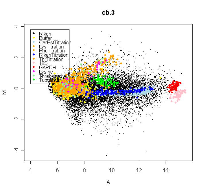
Found 19200 Control
Found 16896 Riken
Found 710 Buffer
Found 192 CerEstTitration
Found 224 LysTitration
Found 260 PheTitration
Found 160 RikenTitration
Found 224 ThrTitration
Found 64 18S
Found 64 GAPDH
Found 32 Lysine
Found 32 Threonine
Found 64 Tubulin
Setting attributes: values col cex
MA-plots were examined for all the arrays. Here we give the plot for array 9 only:
> plotMD(RG,column=9,xlim=c(4,15.5))
Here Buffer is an obvious negative control while 18S, GAPDH, Lysine, Threonine and Tubulin are
single-gene positive controls, sometime called house-keeping genes. RikenTitration is a titration
series of a pool of the entire Riken library, and can be reasonably expected to be non-differentially
expressed. CerEstTitration is a titration of a pool of a cerebellum EST library. This will show higher
expression in later mutant tissues. The Lys, Phe and Thr series are single-gene titration series which
were not spiked-in in this case and can therefore be treated as negative controls.
93
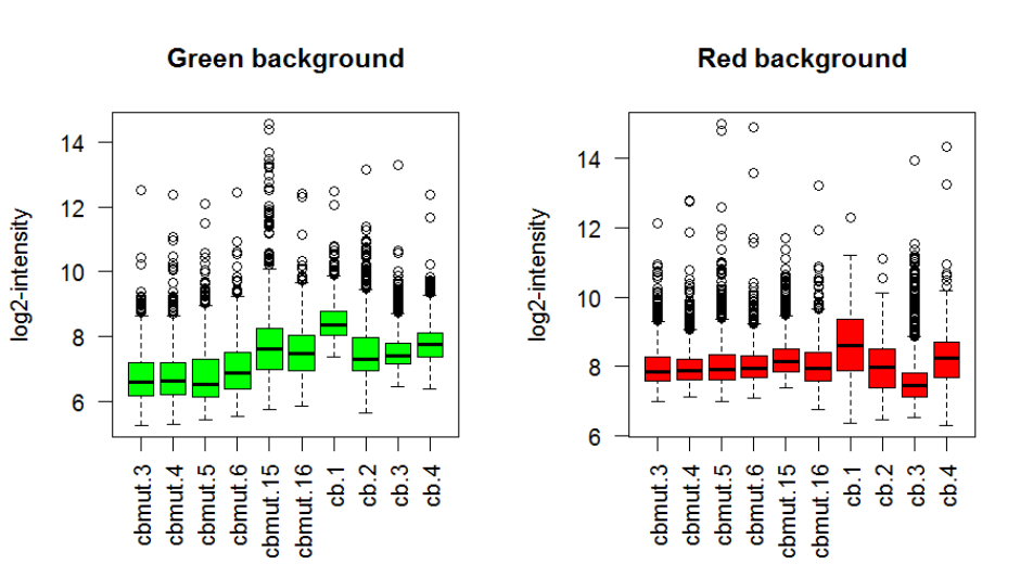
The negative control probe intensities are quite high, especially for the red channel and especially
for array 7:
> negative <- RG$genes$Status %in% c("Buffer","LysTitration","PheTitration","ThrTitration")
> par(mfrow=c(1,2))
> boxplot(log2(RG$G[negative,]),las=2,main="Green background",ylab="log2-intensity",col="green")
> boxplot(log2(RG$R[negative,]),las=2,main="Red background",ylab="log2-intensity",col="red")
> par(mfrow=c(1,1))
Later on, we will investigate setting array quality weights.
Now normalize the data. The Riken titration library, being based on a pool of a large number
of non-specific genes, should not be differentially expressed. We can take advantage of this by
upweighting these probes in the print-tip normalization step. Here we give double-weight to the
titration library probes, although higher weights could also be considered:
> w <- modifyWeights(RG$weights, RG$genes$Status, "RikenTitration", 2)
> MA <- normalizeWithinArrays(RG, weights = w)
16.3.6 Setting Up the Linear Model
The experiment has a composite design, with some arrays comparing back to the RNA pool as a
common reference, and other arrays making direct comparisons between the treatment conditions of
interest. The simplest design matrix is that which compares all the RNA samples back to the RNA
pool.
> design <- modelMatrix(targets, ref = "Pool")
Found unique target names:
P11mt P11wt P21mt P21wt Pool
We also add an intercept term to extract probe-specific dye effects:
94
> design <- cbind(Dye=1,design)
> design
Dye P11mt P11wt P21mt P21wt
cbmut.3 1 0 1 0 0
cbmut.4 1 1 0 0 0
cbmut.5 1 0 0 1 0
cbmut.6 1 0 0 0 1
cbmut.15 1 0 0 0 1
cbmut.16 1 0 0 1 0
cb.1 1 -1 1 0 0
cb.2 1 1 0 -1 0
cb.3 1 0 0 1 -1
cb.4 1 0 -1 0 1
16.3.7 Probe Filtering and Array Quality Weights
First we remove control probes, leaving only the regular probes of the Riken library:
> regular <- MA$genes$Status=="Riken"
> MA2 <- MA[regular,]
> MA2$genes$Status <- NULL
Then we estimate array quality weights:
> aw <- arrayWeights(MA2,design)
> options(digits=3)
> aw
1 2 3 4 5 6 7 8 9 10
1.175 1.457 0.852 1.216 0.371 1.087 1.325 0.856 1.418 0.869
The array weights multiply the spot weights already in the data object:
> library(statmod)
> w <- matvec(MA2$weights,aw)
16.3.8 Differential expression
Fit the linear model:
> fit <- lmFit(MA2, design, weights=w)
Now extract all possible comparisons of interest as contrasts. We look for the mutant vs wt
comparisons at 11 and 21 days, the time effects for mutant and wt, and the interaction terms:
> cont.matrix <- makeContrasts(
+ WT11.MT11=P11mt-P11wt,
+ WT21.MT21=P21mt-P21wt,
+ WT11.WT21=P21wt-P11wt,
+ MT11.MT21=P21mt-P11mt,
+ Int=(P21mt-P11mt)-(P21wt-P11wt),
+ levels=design)
> fit2 <- contrasts.fit(fit, cont.matrix)
> fit2 <- eBayes(fit2)
Adjustment for multiple testing, using Benjamini and Hochberg’s method to control the false dis-
covery rate at 5% across all genes and all contrasts, leads to the following:
95
> results <- decideTests(fit2,method="global")
> summary(results)
WT11.MT11 WT21.MT21 WT11.WT21 MT11.MT21 Int
-1 28 136 455 765 74
0 16835 16540 16102 15377 16692
1 33 220 339 754 130
The probes that show significant interactions are those which develop differently in the mutant
compared to the wild-type between days 11 and 21. To see these:
> topTable(fit2,coef="Int")
RikenID GenBank Symbol logFC AveExpr t P.Value adj.P.Val B
14395 ZX00005I07 AV038977 <NA> 2.71 10.52 11.40 8.56e-08 0.00145 7.66
1473 ZX00028J17 AV076735 <NA> 1.92 11.37 10.11 3.18e-07 0.00215 6.65
14288 ZA00003I15 AV010442 <NA> 2.21 9.50 9.94 3.81e-07 0.00215 6.50
1184 ZX00004J09 AK005530 Tnfrsf12a -2.02 8.47 -9.43 6.74e-07 0.00237 6.03
13843 ZX00003J07 AV033559 <NA> -2.97 12.08 -9.33 7.51e-07 0.00237 5.95
14898 ZX00003H24 AK005382 Tnfrsf12a -2.41 9.40 -9.23 8.43e-07 0.00237 5.86
13520 ZX00020K15 AV088030 <NA> 1.83 9.93 9.09 9.88e-07 0.00238 5.73
10916 ZX00023L14 AV104464 <NA> 2.90 10.49 8.93 1.19e-06 0.00252 5.37
12532 ZX00026E06 AV140268 <NA> 2.75 10.55 8.63 1.71e-06 0.00322 5.27
14250 ZX00048F23 AV122249 <NA> 1.89 10.27 8.41 2.23e-06 0.00377 5.04
> sessionInfo()
R version 2.13.0 Patched (2011-04-25 r55638)
Platform: i386-pc-mingw32/i386 (32-bit)
locale:
[1] LC_COLLATE=English_Australia.1252 LC_CTYPE=English_Australia.1252
[3] LC_MONETARY=English_Australia.1252 LC_NUMERIC=C
[5] LC_TIME=English_Australia.1252
attached base packages:
[1] splines stats graphics grDevices utils datasets methods base
other attached packages:
[1] statmod_1.4.11 org.Mm.eg.db_2.5.0 RSQLite_0.9-4 DBI_0.2-5
[5] AnnotationDbi_1.14.0 Biobase_2.12.0 limma_3.9.8
16.4 Bob1 Mutant Mice: Arrays With Duplicate Spots
In this section we consider a case study in which all genes (ESTs and controls) are printed more
than once on the array. This means that there is both within-array and between-array replication for
each gene. The structure of the experiment is therefore essentially a randomized block experiment
for each gene. The approach taken here is to estimate a common correlation for all the genes for
between within-array duplicates. The theory behind the approach is explained in [32]. This approach
assumes that all genes are replicated the same number of times on the array and that the spacing
between the replicates is entirely regular.
In this example we assume that the data is available as an RGList.
Background. This data is from a study of transcription factors critical to B cell maturation by
Lynn Corcoran and Wendy Dietrich at the WEHI. Mice which have a targeted mutation in the Bob1
(aka Pou2af1 or OBF-1) transcription factor display a number of abnormalities in the B lymphocyte
96
compartment of the immune system. Immature B cells that have emigrated from the bone marrow
fail to differentiate into full fledged B cells, resulting in a notable deficit of mature B cells.
Arrays. Arrays were printed at the Australian Genome Research Facility with expressed sequence
tags (ESTs) from the National Institute of Aging 15k mouse clone library, plus a range of positive,
negative and calibration controls. The arrays were printed using a 48 tip print head and 26x26 spots
in each tip group. Data from 24 of the tip groups are given here. Every gene (ESTs and controls)
was printed twice on each array, side by side by rows. The NIA15k probe IDs have been anonymized
in the output presented here.
Hybridizations. A retrovirus was used to add Bob back to a Bob deficient cell line. Two RNA
sources were compared using 2 dye-swap pairs of microarrays. One RNA source was obtained from
the Bob deficient cell line after the retrovirus was used to add GFP (”green fluorescent protein”,
a neutral protein). The other RNA source was obtained after adding both GFP and Bob protein.
RNA from Bob+GFP was labelled with Cy5 in arrays 2 and 4, and with Cy3 in arrays 1 and 4.
Image analysis. The arrays were image analyzed using SPOT with “morph” background estima-
tion.
The data used for this case study can be downloaded from http://bioinf.wehi.edu.au/limma/.
The file should be placed in the working directory of your R session. (This case study was last updated
on 29 June 2006 using R 2.3.0 and limma 2.7.5.)
> library(limma)
> load("Bob.RData")
> objects()
[1] "design" "RG"
> design
[1] -1 1 -1 1
> names(RG)
[1] "R" "G" "Rb" "Gb" "genes" "printer"
> RG$genes[1:40,]
Library ID
1 Control cDNA1.500
2 Control cDNA1.500
3 Control Printing.buffer
4 Control Printing.buffer
5 Control Printing.buffer
6 Control Printing.buffer
7 Control Printing.buffer
8 Control Printing.buffer
9 Control cDNA1.500
10 Control cDNA1.500
11 Control Printing.buffer
12 Control Printing.buffer
13 Control Printing.buffer
14 Control Printing.buffer
15 Control Printing.buffer
16 Control Printing.buffer
17 Control cDNA1.500
18 Control cDNA1.500
19 Control Printing.buffer
20 Control Printing.buffer
21 Control Printing.buffer
22 Control Printing.buffer
23 Control Printing.buffer
97
24 Control Printing.buffer
25 Control cDNA1.500
26 Control cDNA1.500
27 NIA15k H31
28 NIA15k H31
29 NIA15k H32
30 NIA15k H32
31 NIA15k H33
32 NIA15k H33
33 NIA15k H34
34 NIA15k H34
35 NIA15k H35
36 NIA15k H35
37 NIA15k H36
38 NIA15k H36
39 NIA15k H37
40 NIA15k H37
Although there are only four arrays, we have a total of eight spots for each gene, and more for
the controls. Naturally the two M-values obtained from duplicate spots on the same array are highly
correlated. The problem is how to make use of the duplicate spots in the best way. The approach
taken here is to estimate the spatial correlation between the adjacent spots using REML and then
to conduct the usual analysis of the arrays using generalized least squares.
First normalize the data using print-tip loess regression. The SPOT morph background ensures
that the default background subtraction can be used without inducing negative intensities.
> MA <- normalizeWithinArrays(RG)
Then remove the control probes:
> MA2 <- MA[MA$genes$Library=="NIA15k", ]
Now estimate the spatial correlation. We estimate a correlation term by REML for each gene,
and then take a trimmed mean on the atanh scale to estimate the overall correlation. This command
will probably take at least a few minutes depending on the speed of your computer.
> options(digits=3)
> corfit <- duplicateCorrelation(MA2,design,ndups=2) # A slow computation!
Loading required package: statmod
> corfit$consensus.correlation
[1] 0.575
> boxplot(tanh(corfit$atanh.correlations))
> fit <- lmFit(MA2,design,ndups=2,correlation=corfit$consensus)
> fit <- eBayes(fit)
> topTable(fit, n=30)
98
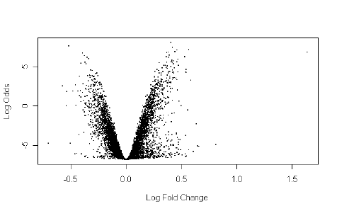
Library ID logFC AveExpr t P.Value adj.P.Val B
4599 NIA15k H34599 0.404 10.93 12.92 1.34e-07 0.000443 8.02
1324 NIA15k H31324 -0.520 7.73 -12.24 2.23e-07 0.000443 7.57
3309 NIA15k H33309 0.420 10.99 11.99 2.71e-07 0.000443 7.39
440 NIA15k H3440 0.568 9.96 11.64 3.60e-07 0.000443 7.13
6795 NIA15k H36795 0.460 10.78 11.56 3.85e-07 0.000443 7.07
121 NIA15k H3121 0.441 10.48 11.31 4.73e-07 0.000443 6.88
2838 NIA15k H32838 1.640 12.74 11.26 4.92e-07 0.000443 6.84
6999 NIA15k H36999 0.381 9.91 11.19 5.21e-07 0.000443 6.79
132 NIA15k H3132 0.370 10.10 11.17 5.31e-07 0.000443 6.77
6207 NIA15k H36207 -0.393 8.53 -11.06 5.82e-07 0.000443 6.69
7168 NIA15k H37168 0.391 9.88 10.76 7.51e-07 0.000493 6.45
1831 NIA15k H31831 -0.374 9.62 -10.63 8.41e-07 0.000493 6.35
2014 NIA15k H32014 0.363 9.65 10.49 9.54e-07 0.000493 6.23
7558 NIA15k H37558 0.532 11.42 10.49 9.58e-07 0.000493 6.22
4471 NIA15k H34471 -0.353 8.76 -10.41 1.02e-06 0.000493 6.16
126 NIA15k H3126 0.385 10.59 10.40 1.03e-06 0.000493 6.15
4360 NIA15k H34360 -0.341 9.37 -10.22 1.21e-06 0.000545 6.00
6794 NIA15k H36794 0.472 11.33 10.11 1.35e-06 0.000570 5.90
329 NIA15k H3329 0.413 11.37 9.97 1.53e-06 0.000612 5.78
5017 NIA15k H35017 0.434 11.41 9.90 1.63e-06 0.000618 5.72
2678 NIA15k H32678 0.461 10.44 9.74 1.90e-06 0.000618 5.57
2367 NIA15k H32367 0.409 10.21 9.72 1.93e-06 0.000618 5.56
1232 NIA15k H31232 -0.372 8.72 -9.70 1.96e-06 0.000618 5.54
111 NIA15k H3111 0.369 10.42 9.69 1.98e-06 0.000618 5.53
2159 NIA15k H32159 0.418 10.19 9.67 2.03e-06 0.000618 5.51
4258 NIA15k H34258 0.299 9.11 9.62 2.12e-06 0.000622 5.47
3192 NIA15k H33192 -0.410 9.46 -9.55 2.26e-06 0.000638 5.41
6025 NIA15k H36025 0.427 10.37 9.47 2.45e-06 0.000654 5.33
5961 NIA15k H35961 -0.362 8.50 -9.46 2.49e-06 0.000654 5.31
1404 NIA15k H31404 0.474 11.34 9.26 3.00e-06 0.000722 5.13
> volcanoplot(fit)
99
Chapter 17
Single-Channel Case Studies
17.1 Lrp Mutant E. Coli Strain with Affymetrix Arrays
17.1.1 Background
Gene expression in two Escherichia coli bacteria strains, labelled lrp+ and lrp-, were compared using
eight Affymetrix E. coli chips, four chips each for lrp+ and lrp-. The data are from experiments
reported in [9], who state that
The purpose of the work presented here is to identify the network of genes that are
differentially regulated by the global E. coli regulatory protein, leucine-responsive regu-
latory protein (Lrp), during steady state growth in a glucose supplemented minimal salts
medium. Lrp is a DNA-binding protein that has been reported to affect the expression
of approximately 55 genes.
17.1.2 Downloading the data
The raw data files can be downloaded from http://bioinf.wehi.edu.au/limma/. The following
code assumes that the files in your current working directory:
> dir()
[1] "Escherichia_coli_str._K-12_substr._MG1655.gene_info.gz" "nolrp_1.CEL"
[3] "nolrp_2.CEL" "nolrp_3.CEL"
[5] "nolrp_4.CEL" "targets.txt"
[7] "wt_1.CEL" "wt_2.CEL"
[9] "wt_3.CEL" "wt_4.CEL"
The file targets.txt describes the design of the experiment:
> library(limma)
> targets <- readTargets("targets.txt")
> targets
FileName Strain Experiment
nolrp_1 nolrp_1.CEL lrp- 1
nolrp_2 nolrp_2.CEL lrp- 2
nolrp_3 nolrp_3.CEL lrp- 3
nolrp_4 nolrp_4.CEL lrp- 4
wt_1 wt_1.CEL lrp+ 1
wt_2 wt_2.CEL lrp+ 2
100
wt_3 wt_3.CEL lrp+ 3
wt_4 wt_4.CEL lrp+ 4
The lrp- samples are from the Lrp-deficient strain while the lrp+ are from the wild-type strain. The
data was collected in four batches or “experiments”.
17.1.3 Background correction and normalization
The data is read and normalized using the affy package. The package ecolicdf must also be installed,
otherwise the rma() function will attempt to download and install it for you.
> library(affy)
> eset <- justRMA(filenames = targets$FileName)
> colnames(eset) <- row.names(targets)
> head(exprs(eset))
nolrp_1 nolrp_2 nolrp_3 nolrp_4 wt_1 wt_2 wt_3 wt_4
aas_b2836_st 8.53 9.20 8.18 8.01 8.89 8.52 8.28 8.11
aat_b0885_st 8.12 8.76 7.96 8.37 7.88 8.61 7.74 8.52
abc_b0199_st 10.65 10.31 10.17 11.60 10.44 10.58 10.20 11.48
abrB_b0715_st 9.32 9.16 9.68 9.20 9.21 9.28 9.65 9.94
accA_b0185_st 11.28 11.38 10.93 10.64 11.22 11.41 11.14 10.82
accB_b3255_st 12.52 11.81 12.32 12.69 12.65 12.29 12.59 12.66
The rownames of the expression matrix combine the gene symbols (aas) with an open reading frame
identifier (b2836). This format is idiosyncratic to this historical GeneChip.
An MDS plot shows clearly that there is a batch effect between the four experiments:
> plotMDS(eset)
−0.5 0.0 0.5 1.0
−0.4 −0.2 0.0 0.2 0.4 0.6 0.8
Leading logFC dim 1
Leading logFC dim 2
nolrp_1
nolrp_2
nolrp_3
nolrp_4
wt_1
wt_2
wt_3
wt_4
17.1.4 Gene annotation
The gene information file Escherichia coli str. K-12 substr. MG1655.gene info.gz was downloaded
from the NCBI ftp site at ftp://ftp.ncbi.nlm.nih.gov/gene/DATA/GENE_INFO. We can use this
file to update the gene annotation.
101
First we extract the old gene symbols from the rownames:
> Alias <- sub("_.*", "", row.names(eset))
> Alias[1:5]
[1] "aas" "aat" "abc" "abrB" "accA"
Then we use limma function alias2SymbolUsingNCBI to update the old gene symbols to current
symbols and associated information. The information is stored in the fData slot of the ExpressionSet:
> GeneInfo <- "Escherichia_coli_str._K-12_substr._MG1655.gene_info.gz"
> fData(eset) <- alias2SymbolUsingNCBI(Alias, GeneInfo,
+ required=c("GeneID","Symbol","type_of_gene"))
> head(fData(eset))
GeneID Symbol type_of_gene
2495 947315 aas protein-coding
719 945490 aat protein-coding
153 944896 metN protein-coding
554 945321 abrB protein-coding
152 944895 accA protein-coding
2922 947758 accB protein-coding
We remove all probes that do not have an Entrez Gene ID and Symbol:
> HasSymbol <- !is.na(fData(eset)$Symbol)
> eset <- eset[HasSymbol,]
> dim(eset)
Features Samples
3709 8
17.1.5 Differential expression
Make factors for the Experiment and Strain:
> Exp <- factor(targets$Experiment)
> Strain <- factor(targets$Strain, levels=c("lrp+","lrp-"))
Then construct the design matrix, with Experiment and Strain. This will allow us to test for Strain
differences adjusting for differences between the Experiments:
> design <- model.matrix(~Exp+Strain)
Now we can run the differential expression pipeline:
> fit <- lmFit(eset, design)
> fit <- eBayes(fit, trend=TRUE, robust=TRUE)
> results <- decideTests(fit)
> summary(results)
(Intercept) Exp2 Exp3 Exp4 Strainlrp-
Down 0 92 382 714 101
NotSig 0 3601 3249 2859 3526
Up 3709 16 78 136 82
There are 82 up-regulated and 101 down-regulated genes in the Lrp- strain at FDR< 0.05. Including
Experiment as a batch was also clearly important.
The top 30 differentially expressed genes can be seen:
102
> topTable(fit, coef="Strainlrp-", n=30)
GeneID Symbol type_of_gene logFC AveExpr t P.Value adj.P.Val B
oppA_b1243_st 945830 oppA protein-coding 2.976 12.97 24.64 7.39e-12 1.33e-08 17.11
rmf_b0953_st 945567 rmf protein-coding 2.705 13.64 24.08 9.74e-12 1.33e-08 16.89
ytfK_b4217_st 948736 ytfK protein-coding 2.641 11.10 23.88 1.08e-11 1.33e-08 16.80
oppB_b1244_st 945823 oppB protein-coding 2.913 10.70 21.57 3.67e-11 3.40e-08 15.77
serA_b2913_st 945258 serA protein-coding -2.776 12.22 -21.13 4.71e-11 3.50e-08 15.56
ompT_b0565_st 945185 ompT protein-coding -2.673 10.52 -20.25 7.86e-11 4.86e-08 15.11
gltD_b3213_st 947723 gltD protein-coding -3.033 10.92 -19.35 1.40e-10 7.44e-08 14.60
ydgR_b1634_st 947436 dtpA protein-coding 2.348 9.78 16.90 6.79e-10 3.15e-07 13.16
pntB_b1602_st 946144 pntB protein-coding -1.470 12.76 -14.66 3.61e-09 1.49e-06 11.59
gltB_b3212_st 947724 gltB protein-coding -3.236 10.05 -16.95 6.07e-09 2.25e-06 11.12
lrp_b0889_st 949051 lrp protein-coding -2.304 9.33 -13.74 7.73e-09 2.61e-06 10.85
oppD_b1246_st 945802 oppD protein-coding 1.944 10.36 12.86 1.66e-08 5.13e-06 10.11
stpA_b2669_st 947130 stpA protein-coding -1.789 10.04 -12.25 2.89e-08 8.18e-06 9.56
livK_b3458_st 947964 livK protein-coding -2.352 9.85 -13.11 3.09e-08 8.18e-06 9.55
ilvC_b3774_st 948286 ilvC protein-coding -1.541 12.94 -11.40 7.31e-08 1.81e-05 8.65
sodA_b3908_st 948403 sodA protein-coding -1.505 10.32 -10.26 2.14e-07 4.97e-05 7.56
ptsG_b1101_st 945651 ptsG protein-coding -1.156 12.17 -10.10 2.55e-07 5.55e-05 7.39
ndk_b2518_st 945611 ndk protein-coding -1.066 11.06 -9.82 3.51e-07 7.22e-05 7.06
pntA_b1603_st 946628 pntA protein-coding -1.585 10.12 -9.57 4.71e-07 9.20e-05 6.76
oppC_b1245_st 945810 oppC protein-coding 2.146 10.71 10.97 1.33e-06 2.28e-04 5.99
ilvH_b0078_st 947267 ilvH protein-coding -1.110 9.94 -8.87 1.05e-06 1.96e-04 5.94
glnA_b3870_st 948370 glnA protein-coding -1.246 12.06 -8.63 1.41e-06 2.28e-04 5.65
livH_b3457_st 947965 livH protein-coding -1.240 9.19 -8.63 1.41e-06 2.28e-04 5.65
artI_b0863_st 948988 artI protein-coding 1.114 12.45 8.48 1.72e-06 2.65e-04 5.45
clpA_b0882_st 945764 clpA protein-coding 0.906 11.90 8.35 2.02e-06 2.91e-04 5.28
dnaK_b0014_st 944750 dnaK protein-coding 0.722 13.45 8.34 2.04e-06 2.91e-04 5.27
ybfA_b0699_st 947452 ybfA protein-coding 0.911 10.54 8.00 3.18e-06 4.37e-04 4.81
livM_b3456_st 947966 livM protein-coding -1.041 8.45 -7.83 3.97e-06 5.26e-04 4.59
yhiP_b3496_st 948006 dtpB protein-coding 1.189 8.52 7.62 5.28e-06 6.76e-04 4.29
livF_b3454_st 947961 livF protein-coding -1.004 9.28 -7.57 5.62e-06 6.83e-04 4.23
Lrp itself is the 11th gene in the list.
We can plot the fold-changes for the significant genes:
> plotMD(fit, coef="Strainlrp-", status=results)
103
8 10 12 14
−3 −2 −1 0 1 2 3
Average log−expression
log−fold−change
●
●
●
●
●
●
●
●
●
●
●
●
●
●
●
●
●
●
●
●
●
●
●
●
●
●
●
●
●
●
●
●
●
●
●
●
●
●
●
●
●
●
●
●
●
●
●
●
●
●
●
●
●●●●
●
●
●
●
●
●
●
●
●
●
●
●
●
●
●
●
●
●
●
●
●
●
●
●
●
●
●
●
●
●
●
●
●
●
●
●
●
●
●
●
●
●
●
●
●
●
●
●
●
●
●
●
●
●
●
●
●
●
●
●
●
●
●
●
●
●
●
●
●
●
●
●
●
●
●
●
●
●
●
●
●
●
●
●
●
●
●
●
●
●
●
●●
●
●
●
●
●
●
●
●
●
●
●
●
●
●
●
●
●
●
●
●
●
●
●
●
●
●
●
●
●
●
●
●
●
●
●
●
●
●
●
●
●
●
●
●
●
●
●
●
●
●
●
●
●
●
●
●
●
●
●
●
●
●
●
●
●
●
●
●
●
●
●
●
●
●
●
●
●
●
●
●
●
●
●
●
●
●
●
●
●
●
●
●
●
●
●
●
●
●
●
●
●
●
●
●
●
●
●
●
●
●
●
●
●
●
●
●
●
●
●
●
●
●
●
●
●
●
●
●
●
●
●
●
●
●
●
●
●
●
●
●
●
●
●
●
●
●
●
●
●
●
●
●
●
●
●
●
●
●
●
●
●
●
●
●
●
●
●
●
●
●
●
●
●
●
●
●
●
●
●
●
●
●
●
●
●
●
●
●
●
●
●
●
●
●
●
●
●
●
●
●
●
●
●
●
●
●
●
●
●
●
●
●
●
●
●
●
●
●
●
●
●
●
●
●
●
●
●
●
●
●
●
●
●
●
●
●
●
●
●
●
●
●
●
●
●
●
●
●
●
●
●
●
●
●
●
●
●
●
●
●
●
●
●
●
●
●
●
●
●
●
●
●
●
●
●
●
●
●
●
●
●
●
●
●
●
●
●
●
●
●
●
●
●
●
●
●
●
●
●
●
●
●
●
●
●
●
●
●
●
●
●
●
●
●
●
●
●
●
●
●
●
●
●
●
●
●
●
●
●
●
●
●
●
●
●
●
●
●
●
●
●
●
●
●
●
●
●
●
●
●
●
●
●
●
●
●
●
●
●
●
●
●
●
●
●
●
●
●
●
●
●
●
●
●
●
●
●
●
●
●
●
●
●
●
●
●
●
●
●
●
●
●
●
●
●
●
●
●
●
●
●
●
●
●
●
●
●
●
●
●
●
●
●
●
●
●
●
●
●
●
●
●
●
●
●
●
●
●
●
●
●
●
●
●
●
●
●
●
●
●
●
●
●
●
●
●
●
●
●
●
●
●
●
●
●
●
●
●
●
●
●
●
●
●
●
●
●
●
●
●
●
●
●
●
●
●
●
●
●
●
●
●
●
●
●
●
●
●
●
●
●
●
●
●
●
●
●
●
●
●
●
●
●
●
●
●
●
●
●
●
●
●
●
●
●
●
●
●
●
●
●
●
●
●
●
●
●
●
●
●
●
●
●
●
●
●
●
●
●
●
●
●
●
●
●
●
●
●
●
●
●
●
●
●
●
●
●
●
●●●●
●
●
●
●
●
●
●
●
●
●●●●
●
●
●
●
●
●
●
●
●
●
●
●
●
●
●
●
●
●
●
●
●
●
●
●
●
●
●
●
●
●
●
●
●
●
●
●
●
●
●
●
●
●
●
●
●
●
●
●
●
●
●
●
●
●
●
●
●
●
●
●
●
●
●
●
●
●
●
●
●
●
●
●
●
●
●
●
●
●
●
●
●
●
●
●
●
●
●
●
●
●
●
●
●
●
●
●
●
●
●
●
●
●
●
●
●
●
●
●
●
●
●
●
●
●
●
●
●
●
●
●
●
●
●
●
●
●
●
●
●
●
●
●
●
●
●
●
●
●
●
●
●
●
●
●
●
●
●
●
●
●
●
●
●
●
●
●
●
●
●
●
●
●
●
●
●
●
●
●
●
●●
●
●
●
●
●
●
●
●
●
●
●
●
●
●
●
●
●
●
●
●
●
●
●
●
●
●
●
●
●
●
●
●
●
●
●
●
●
●
●
●
●
●
●
●
●
●
●
●
●
●
●
●
●
●
●
●
●
●
●
●
●
●
●
●
●
●
●
●
●
●
●
●
●
●
●
●
●
●
●
●
●
●
●
●
●
●
●
●
●
●
●
●
●
●
●
●
●
●
●
●
●
●
●
●
●
●
●
●
●
●
●
●
●
●
●
●
●
●
●
●
●
●
●
●
●
●
●
●
●
●
●
●
●
●
●
●
●
●
●
●
●
●
●
●
●
●
●
●
●
●
●
●
●
●
●
●
●
●
●
●
●
●
●
●
●
●
●
●
●
●
●
●
●
●
●
●
●
●
●
●
●
●
●
●
●
●
●
●
●
●
●
●
●
●
●
●
●
●
●
●
●
●
●
●
●
●
●
●
●
●
●
●
●
●
●
●
●
●
●
●
●
●
●
●
●
●
●
●
●
●
●
●
●
●
●
●
●
●
●
●
●
●
●
●
●
●
●
●
●
●
●
●
●
●
●
●
●
●
●
●
●
●
●
●
●
●
●
●
●
●
●
●
●
●
●
●
●
●
●
●
●
●
●
●
●
●
●
●
●
●
●
●
●
●
●
●
●
●
●
●
●
●
●
●
●
●
●
●
●
●
●
●
●
●
●
●
●
●
●
●
●
●
●
●
●
●
●
●
●
●
●
●
●
●
●
●
●
●
●
●
●
●
●
●
●
●
●
●
●
●
●
●
●
●
●
●
●
●
●
●
●
●
●
●
●
●
●
●
●
●
●
●
●
●
●
●
●
●
●
●
●
●
●
●
●
●
●
●
●
●
●
●
●
●
●
●
●
●
●
●
●
●
●
●
●
●
●
●
●
●
●
●
●
●
●
●
●
●
●
●
●
●
●
●
●
●
●
●
●
●
●
●
●
●
●
●
●
●
● ●
●
●
●
●
●
●
●
●
●
●
●
●
●
●
●
●
●
●
●
●
●
●
●
●
●
●
●
●
●
●
●
●
●
●
●
●
●
●
●
●
●
●
●
●
●
●
●
●
●
●
●
●
●
●
●
●
●
●
●
●
●
●
●
●
●
●
●
●
●
●
●
●
●
●
●
●
●
●
●
●
●
●
●
●
●
●
●
●
●
●
●
●
●
●
●
●
●
●
●
●
●
●
●
●
●
●
●
●
●
●
●
●
●
●
●
●
●
●
●
●
●
●
●
●
●
●
●
●
●
●
●
●
●
●
●
●
●
●
●
●
●
●
●
●
●
●
●
●
●
●
●
●
●
●
●
●
●
●
●
●
●
●
●
●
●
●
●
●
●
●
●
●
●
●
●
●
●
●
●
●
●
●
●
●
●
●
●
●
●
●
●
●
●
●
●
●
●
●
●
●
●
●
●
●
●
●
●
●
●
●
●
●
●
●
●
●
●
●
●
●
●
●
●
●
●
●
●
●
●
●
●
●
●
●
●
●
●
●
●
●
●
●
●
●
●
●
●
●
●
●
●
●
●
●
●
●
●
●
●
●
●
●
●
●
●
●
●
●
●
●
●
●
●
●
●
●
●
●
●
●
●
●
●
●
●
●
●
●
●
●
●
●
●
●
●
●
●
●
●
●
●
●
●
●
●
●
●
●
●
●
●
●
●
●
●
●
●
●
●
●
●
●●●●
●
●
●
●
●
●
●
●
●
●
●
●
●
●
●
●
●
●
●
●
●
●
●
●
●
●
●
●
●
●
●
●
●
●
●
●
●
●
●
●
●
●
●
●
●
●
●
●
●
●
●
●
●
●
●
●
●
●
●
●
●
●
●
●
●
●
●
●
●
●
●●
●
●
●
●
●
●
●
●
●
●
●
●
●
●
●
●
●
●
●
●
●
●
●
●
●
●
●
●
●
●
●
●
●
●
●
●
●
●
●
●
●
●
●
●
●
●
●
●
●
●
●
●
●
●
●
●
●
●
●
●
●
●
●
●
●
●
●
●
●
●
●
●
●
●
●
●
●
●
●
●
●
●
●
●
●
●
●
●
●
●
●
●
●
●
●
●
●
●
●
●
●
●
●
●
●
●
●
●
●
●
●
●
●
●
●
●
●
●
●
●
●
●
●
●
●
●
●
●
●
●
●
●
●
●
●
●
●
●
●
●
●
●
●
●
●
●
●
●
●
●
●
●
●
●
●
●
●
●
●
●
●
●
●
●
●
●
●
●
●
●●●
●
●
●
●
●
●
●
●
●
●
●
●
●
●
●
●
●
●
●
●
●
●
●
●
●
●
●
●
●
●
●
●
●
●
●
●
●
●
●
●
●
●
●
●
●
●
●
●
●
●
●
●
●
●
●
●
●
●
●
●
●
●
●
●
●
●
●
●
●
●
●
●
●
●
●
●
●
●
●
●
●
●
●
●
●
●
●
●
●
●
●
●
●
●
●
●
●
●
●
●
●
●
●
●
●●
●
●
●
●
●
●
●
●
●
●
●
●
●
●
●
●
●
●
●
●
●
●
●
●
●
●
●
●
●
●
●
●
●
●
●
●
●
●
●
●
●
●
●
●
●
●
●
●
●
●
●
●
●
●
●
●
●
●
●
●
●
●
●
●
●
●
●
●
●
●
●
●
●
●
●
●
●
●
●
●
●
●
●
●
●
●
●
●
●
●
●
●
●
●
●
●
●
●
●
●
●
●
●
●
●
●
●
●
●
●
●
●
●
●
●
●
●
●
●
●
●
●
●
●
●
●
●
●
●
●
●
●
●
●
●
●
●
●
●
●
●
●
●
●
●
●
●
●
●
●
●
●
●
●
●
●
●
●
●
●
●
●
●
●
●
●
●
●
●
●
●
●
●
●
●
●
●
●
●
●
●
●
●
●
●
●
●
●
●
●
●
●
●
●
●
●
●
●
●
●
●
●
●
●
●
●
●
●
●
●
●
●
●
●
●
●
●
●
●
●
●
●
●
●
●
●
●
●
●
●
●
●
●
●
●
●
●
●
●
●
●
●
●
●
●
●
●
●
●
●
●
●
●
●
●
●
●
●
●
●
●
●
●
●
●
●
●
●
●
●
●
●
●
●
●
●
●
●
●
●
●
●
●
●
●
●
●
●
●
●
●
●
●
●
●
●
●
●
●
●
●
●
●
●
●
●
●
●
●
●
●
●
●
●
●
●
●
●
●
●
●
●
●
●
●
●
●
●
●
●
●
●
●
●
●
●
●
●
●
●
● ●
●
●
●
●
●
●
●
●
●
●
●
●
●
●
●
●
●
●
●
●
●
●
●
●
●
●
●
●
●
●
●
●
●
●
●
●
●
●
●
●
●
●
●
●
●
●
●
●
●
●
●
●
●
●
●
●
●
●
●
●
●
●
●
●
●
●
●
●
●
●
●
●
●
●
●
●
●
●
●
●
●
●
●
●
●
●
●
●
●
●
●
●
●
●
●
●
●
●
●
●
●
●
●
●
●
●
●
●
●
●
●
●
●
●
●
●
●
●
●
●
●
●
●
●
●
●
●
●
●
●
●
●
●
●
●
●
●
●
●
●
●
●
●
●
●
●
●
●
●
●
●
●
●
●
●
●
●
●
●
●
●
●
●
●
●
●
●
●
●
●
●
●
●
●
●
●
●
●
●
●
●
●
●
●
●
●
●
●
●
●
●
●
●●
●
●
●
●
●
●
●
●
●
●
●
●
●
●
●
●
●
●
●
●
●
●
●
●
●
●
●
●
●
●
●
●
●
●
●
●
●
●
●
●
●
●
●
●
●
●
●
●
●
●
●
●
●
●
●
●
●
●
●
●
●
●
●
●
●
●
●
●
●
●
●
●
●
●
●
●
●
●
●
●
●
●
●
●
●
●
●
●
●
●
●
●
●
●
●
●
●
●
●
●
●
●
●
●
●
●
●
●
●
●
●
●
●
●
●
●
●
●
●
●
●
●
●
●
●
●
●
●
●
●
●
●
●
●
●
●
●
●
●
●
●
●
●
●
●
●
●
●
●
●
●
●
●
●
●
●
●
●
●
●
●
●
●
●
●
●
●
●
●
●
●
●
●
●
●
●
●
●
●
●
●
●
●
●
●
●
●
●
●
●
●
●
●
●
●
●
●
●
●
●
●
●
●
●
●
●
●
●
●
●
●
●
●
●
●
●
●
●
●
●
●
●
●
●
●
●
●
●
●
●
●
●
●
●
●
●
●
●
●
●
●
●
●
●
●
●
●
●
●
●
●
●
●
●
●
●
●
●
●
●
●
●
●
●
●
●
●
●
●
●
●
●
●
●
●
●
●
●
●
●
●
●
●
●
●
●
●
●
●
●
●
●
●
●
●
●
●
●
●
●
●
●
●
●
●
●
●
●
●
●
●
●
●
●
●
●
●
●
●
●
●
●
●
●
●
●
●
●
●
●
●
●
●
●
●
●
●
●
●
●
●
●
●
●
●
●
●
●
●
●
●
●
●
●
●
●
●
●
●
●
●
●
●
●
●
●
●
●
●
●
●
●
●
●
●
●
●
●
●
●
●
●
●
●
●
●
●
●
●
●
●
●
●
●
●
●
●
●
●
●
●
●
●
●
●
●
●
●
●
●
●
●
●
●
●
●
●
●
●
●
●
●
●
●
●
●
●
●
●
●
●
●
●
●
●
●
●
●
●
●
●
●
●
●
●
●
●
●
●
●
●
●
●
●
●
●
●
●
●
●
●
●
●
●
●
●
●
●
●
●
●
●
●
●
●
●
●
●
●
●
●
●
●
●
●
●
●
●
●
●
●
●
●
●
●
●
●
●
●
●
●
●
●
●
●
●
●
●
●
●
●
●
●
●
●
●
●
●
●
●
●
●
●
●
●
●
●
●
●
●
●
●
●
●
●
●
●
●
●
●
●
●
●
●
●
●
●
●
●
●
●
●
●
●
●
●
●
●
●
●
●
●
●
●
●
●
●
●
●
●
●
●
●
●
●
●
●
●
●
●
●
●
●
●
●
●
●
●
●
●
●
●
●
●
●
●
●
●
●
●
●
●
●
●
●
●
●
●
●
●
●
●
●
●
●
●
●
●
●
●
●
●
●
●
●
●
●
●
●
●
●
●
●
●
●
●
●
●
●
●
●
●
●
●
●
●
●
●
●
●
●
●
●
●
●
●
●
●
●
●
●
●
●
●
●
●
●
●
●
●
●
●
●
●
●
●
●
●
●
●
●
●
●
●
●
●
●
●
●
●
●
●
●
●
●
●
●
●
●
●
●
●
●
●
●
●
●
●
●
●
●
●
●
●
●
●
●
●
●
●
●
●
●
●
●
●
●
●
●
●
●
●
●
●
●
●
●
●
●
●
●
●
●
●
●
●
●
●
●
●
●
●
●
●
●
●
●
●
●
●
●
●
●
●
●
●
●
●
●
●
●
●
●
●
●
●
●
●
●
●
●
●
●
●
●
●
●
●
●
●
●
●
●
●
●
●
●
●
●
●
●
●
●
●
●
●
●
●
●
●
●
●
●
●
●
●
●
●
●
●
●
●
●
●
●
●
●
●
●
●
●
●
●
●
●
●
●
●
●
●
●
●
●
●
●
●
●
●
●
●
●
●
●
●
●
●
●
●
●
●
●
●
●
●
●
●
●
●
●
●
●
●
●
●
●
●
●
●
●
●
●
●
●
●
●
●
●
●
●
●
●
●
●
●
●
●
●
●
●
●
●
●
●
●
●
●
●
●
●
●
●
●
●
●
●
●
●
●
●
●
●
●
●
●
●
●
●
●
●
●
●
●
●
●
●
●
●
●
●
●
●
●
●
●
●
●
●
●
●
●
●
●
●
●
●
●
●
●
●
●
●
●
●
●
●
●
●
●
●
●
●
●
●
●
●
●
●
●
●
●
●
●
●
●
●
●
●
●
●
●
●
●
●
●
●
●
●
●
●
●
●
●
●
●
●
●
●
●
●
●
●
●
●
●
●
NotSig
Up
Down
17.2 Effect of Estrogen on Breast Cancer Tumor Cells: A 2x2 Fac-
torial Experiment with Affymetrix Arrays
This data is from the estrogen package on Bioconductor. A subset of the data is also analyzed in the
factDesign package vignette. To repeat this case study you will need to have the R packages affy,
estrogen and hgu95av2cdf installed.
The data gives results from a 2x2 factorial experiment on MCF7 breast cancer cells using
Affymetrix HGU95av2 arrays. The factors in this experiment were estrogen (present or absent)
and length of exposure (10 or 48 hours). The aim of the study is the identify genes which respond to
estrogen and to classify these into early and late responders. Genes which respond early are putative
direct-target genes while those which respond late are probably downstream targets in the molecular
pathway.
First load the required packages:
> library(limma)
> library(affy)
Welcome to Bioconductor
Vignettes contain introductory material. To view,
simply type: openVignette()
For details on reading vignettes, see
the openVignette help page.
> library(hgu95av2cdf)
The data files are contained in the extdata directory of the estrogen package:
> datadir <- file.path(.find.package("estrogen"),"extdata")
> dir(datadir)
[1] "00Index" "bad.cel" "high10-1.cel" "high10-2.cel" "high48-1.cel"
[6] "high48-2.cel" "low10-1.cel" "low10-2.cel" "low48-1.cel" "low48-2.cel"
[11] "phenoData.txt"
104
The targets file is called phenoData.txt. We see there are two arrays for each experimental
condition, giving a total of 8 arrays.
> targets <- readTargets("phenoData.txt",path=datadir,sep="",row.names="filename")
> targets
filename estrogen time.h
low10-1 low10-1.cel absent 10
low10-2 low10-2.cel absent 10
high10-1 high10-1.cel present 10
high10-2 high10-2.cel present 10
low48-1 low48-1.cel absent 48
low48-2 low48-2.cel absent 48
high48-1 high48-1.cel present 48
high48-2 high48-2.cel present 48
Now read the cel files into an AffyBatch object and normalize using the rma() function from the
affy package:
> ab <- ReadAffy(filenames=targets$filename, celfile.path=datadir)
> eset <- rma(ab)
Background correcting
Normalizing
Calculating Expression
By default, the only probe-set annotation contained in eset is the Affymetrix ID number. We
will add gene symbols to the data object now, so that they will be automatically included in limma
results tables later on.
> library(annotate)
Loading required package: AnnotationDbi
> library(hgu95av2.db)
Loading required package: org.Hs.eg.db
Loading required package: DBI
> ID <- featureNames(eset)
> Symbol <- getSYMBOL(ID,"hgu95av2.db")
> fData(eset) <- data.frame(Symbol=Symbol)
There are many ways to construct a design matrix for this experiment. Given that we are
interested in the early and late estrogen responders, we can choose a parametrization which includes
these two contrasts.
> treatments <- factor(c(1,1,2,2,3,3,4,4),labels=c("e10","E10","e48","E48"))
> contrasts(treatments) <- cbind(Time=c(0,0,1,1),E10=c(0,1,0,0),E48=c(0,0,0,1))
> design <- model.matrix(~treatments)
> colnames(design) <- c("Intercept","Time","E10","E48")
The second coefficient picks up the effect of time in the absence of estrogen. The third and fourth
coefficients estimate the log
2
-fold change for estrogen at 10 hours and 48 hours respectively.
> fit <- lmFit(eset,design)
We are only interested in the estrogen effects, so we choose a contrast matrix which picks these
two coefficients out:
> cont.matrix <- cbind(E10=c(0,0,1,0),E48=c(0,0,0,1))
> fit2 <- contrasts.fit(fit, cont.matrix)
> fit2 <- eBayes(fit2)
105
We can examine which genes respond to estrogen at either time using the moderated F -statistics on
2 degrees of freedom. The moderated F p-value is stored in the component fit2$F.p.value.
What p-value cutoff should be used? One way to decide which changes are significant for each
gene would be to use Benjamini and Hochberg’s method to control the false discovery rate across all
the genes and both tests:
> results <- decideTests(fit2, method="global")
Another method would be to adjust the F-test p-values rather than the t-test p-values:
> results <- decideTests(fit2, method="nestedF")
Here we use a more conservative method which depends far less on distributional assumptions, which
is to make use of control and spike-in probe-sets which theoretically should not be differentially-
expressed. The smallest p-value amongst these controls turns out to be about 0.00014:
> i <- grep("AFFX",featureNames(eset))
> summary(fit2$F.p.value[i])
Min. 1st Qu. Median Mean 3rd Qu. Max.
0.0001391 0.1727000 0.3562000 0.4206000 0.6825000 0.9925000
So a cutoff p-value of 0.0001, say, would conservatively avoid selecting any of the control probe-sets
as differentially expressed:
> results <- classifyTestsF(fit2, p.value=0.0001)
> summary(results)
E10 E48
-1 40 76
0 12469 12410
1 116 139
> table(E10=results[,1],E48=results[,2])
E48
E10 -1 0 1
-1 29 11 0
0 47 12370 52
1 0 29 87
> vennDiagram(results,include="up")
E10 E48
12457
5229 87
106
> vennDiagram(results,include="down")
E10 E48
12538
4711
29
We see that 87 genes were up regulated at both 10 and 48 hours, 29 only at 10 hours and 52 only
at 48 hours. Also, 29 genes were down-regulated throughout, 11 only at 10 hours and 47 only at 48
hours. No genes were up at one time and down at the other.
topTable gives a detailed look at individual genes. Estrogen effect at 10 hours:
> options(digits=3)
> topTable(fit2,coef="E10",n=20)
Symbol logFC AveExpr t P.Value adj.P.Val B
39642_at ELOVL2 2.94 7.88 23.7 4.74e-09 3.13e-05 9.97
910_at TK1 3.11 9.66 23.6 4.96e-09 3.13e-05 9.94
31798_at TFF1 2.80 12.12 16.4 1.03e-07 3.51e-04 7.98
41400_at TK1 2.38 10.04 16.2 1.11e-07 3.51e-04 7.92
40117_at MCM6 2.56 9.68 15.7 1.47e-07 3.58e-04 7.71
1854_at MYBL2 2.51 8.53 15.2 1.95e-07 3.58e-04 7.49
39755_at XBP1 1.68 12.13 15.1 2.05e-07 3.58e-04 7.45
1824_s_at PCNA 1.91 9.24 14.9 2.27e-07 3.58e-04 7.37
1126_s_at CD44 1.78 6.88 13.8 4.12e-07 5.78e-04 6.89
1536_at CDC6 2.66 5.94 13.3 5.80e-07 7.32e-04 6.61
981_at MCM4 1.82 7.78 13.1 6.46e-07 7.42e-04 6.52
33252_at MCM3 1.74 8.00 12.6 8.86e-07 9.20e-04 6.25
1505_at TYMS 2.40 8.76 12.5 9.48e-07 9.20e-04 6.19
34363_at SEPP1 -1.75 5.55 -12.2 1.14e-06 1.03e-03 6.03
1884_s_at PCNA 2.80 9.03 12.1 1.26e-06 1.06e-03 5.95
36134_at OLFM1 2.49 8.28 11.8 1.50e-06 1.19e-03 5.79
37485_at SLC27A2 1.61 6.67 11.4 1.99e-06 1.48e-03 5.55
239_at CTSD 1.57 11.25 10.4 4.07e-06 2.66e-03 4.90
38116_at KIAA0101 2.32 9.51 10.4 4.09e-06 2.66e-03 4.90
40533_at BIRC5 1.26 8.47 10.4 4.21e-06 2.66e-03 4.87
Estrogen effect at 48 hours:
107
> topTable(fit2,coef="E48",n=20)
Symbol logFC AveExpr t P.Value adj.P.Val B
910_at TK1 3.86 9.66 29.2 8.27e-10 1.04e-05 11.61
31798_at TFF1 3.60 12.12 21.0 1.28e-08 7.63e-05 9.89
1854_at MYBL2 3.34 8.53 20.2 1.81e-08 7.63e-05 9.64
38116_at KIAA0101 3.76 9.51 16.9 8.12e-08 2.51e-04 8.48
38065_at HMGB2 2.99 9.10 16.2 1.12e-07 2.51e-04 8.21
39755_at XBP1 1.77 12.13 15.8 1.36e-07 2.51e-04 8.05
1592_at TOP2A 2.30 8.31 15.8 1.39e-07 2.51e-04 8.03
41400_at TK1 2.24 10.04 15.3 1.81e-07 2.75e-04 7.81
33730_at GPRC5A -2.04 8.57 -15.1 1.96e-07 2.75e-04 7.74
1651_at UBE2C 2.97 10.50 14.8 2.39e-07 3.02e-04 7.57
38414_at CDC20 2.02 9.46 14.6 2.66e-07 3.05e-04 7.48
1943_at CCNA2 2.19 7.60 14.0 3.72e-07 3.69e-04 7.18
40117_at MCM6 2.28 9.68 14.0 3.80e-07 3.69e-04 7.17
40533_at BIRC5 1.64 8.47 13.5 4.94e-07 4.45e-04 6.93
39642_at ELOVL2 1.61 7.88 13.0 6.71e-07 5.18e-04 6.65
34851_at AURKA 1.96 9.96 12.8 7.51e-07 5.18e-04 6.55
1824_s_at PCNA 1.64 9.24 12.8 7.95e-07 5.18e-04 6.50
35995_at ZWINT 2.76 8.87 12.7 8.32e-07 5.18e-04 6.46
893_at UBE2S 1.54 10.95 12.7 8.43e-07 5.18e-04 6.45
40079_at GPRC5A -2.41 8.23 -12.6 8.62e-07 5.18e-04 6.42
> sessionInfo()
R version 3.0.0 (2013-04-03)
Platform: i386-w64-mingw32/i386 (32-bit)
locale:
[1] LC_COLLATE=English_Australia.1252 LC_CTYPE=English_Australia.1252
[3] LC_MONETARY=English_Australia.1252 LC_NUMERIC=C
[5] LC_TIME=English_Australia.1252
attached base packages:
[1] parallel stats graphics grDevices utils datasets methods base
other attached packages:
[1] hgu95av2.db_2.9.0 org.Hs.eg.db_2.9.0 RSQLite_0.11.3
[4] DBI_0.2-6 annotate_1.38.0 hgu95av2cdf_2.12.0
[7] AnnotationDbi_1.22.2 affy_1.38.1 Biobase_2.20.0
[10] BiocGenerics_0.6.0 limma_3.17.7 BiocInstaller_1.10.0
loaded via a namespace (and not attached):
[1] affyio_1.28.0 IRanges_1.18.0 preprocessCore_1.22.0
[4] stats4_3.0.0 tools_3.0.0 XML_3.96-1.1
[7] xtable_1.7-1 zlibbioc_1.6.0
17.3 Comparing Mammary Progenitor Cell Populations with Illu-
mina BeadChips
17.3.1 Introduction
This case study examines the expression profiles of adult mammary stem cells and of progenitor
and mature mammary luminal cells. The data was first published by Lim et al [16], who used the
expression profiles to show that luminal progenitor cells are the likely cell of origin for basal-like
breast cancer.
108
The data files used in this case study can be downloaded from http://bioinf.wehi.edu.au/
marray/IlluminaCaseStudy. The expression data files are provided as gzip files and will need to
be uncompressed before they can be used for a limma analysis. To run the analysis described here,
download and unzip the data files and set the working directory of R to the folder containing the
files.
17.3.2 The target RNA samples
The data consists of three files:
> dir()
[1] "control probe profile.txt"
[2] "probe profile.txt"
[3] "Targets.txt"
First read the targets file describing the target RNA samples.
> library(limma)
> targets <- readTargets()
> targets
Donor Age CellType
1 1 39 MS
2 1 39 Stroma
3 1 39 ML
4 1 39 LP
5 2 57 MS
6 2 57 Stroma
7 2 57 ML
8 2 57 LP
9 3 21 MS
10 3 21 Stroma
11 3 21 ML
12 3 21 LP
Breast tissue was obtained from three healthy human donors who were undergoing reduction mam-
moplasties. Epithelial cells were sorted into three subpopulations enriched for mammary stem cells
(MS), luminal progenitor cells (LP) and mature luminal cells (ML) [16]. The MS, LP and ML cells
representative a lineage of luminal cells use to construct the ducts used to transport milk in the
breast [37]:
Stromal cells were also profiles as a comparison group. There were therefore four cell populations
from each person. RNA was extracted from freshly sorted cells, making twelve RNA samples in
total.
109
17.3.3 The expression profiles
The RNA samples were hybridized to two Illumina HumanWG-6 version 3 BeadChips. Each Bead-
Chip is able to accommodate six samples. The BeadChips images were scanned and summarized
using BeadStudio. Un-normalized summary probe profiles were exported from BeadStudio to tab-
delimited text files.
Separate files were written for regular probes and for control probes. The file probe profile.txt
contains the expression profiles for regular probes, designed to interrogate the expression levels of
genes. control probe profile.txt contains the profiles of control probes, including negative control
probes. Note that BeadStudio by default writes the profiles for all the samples to the same two files.
We read in the expression profiles for both regular and control probes, telling read.ilm that we
wish to read the detection p-values as well as the expression values:
> x <- read.ilmn(files="probe profile.txt",ctrlfiles="control probe profile.txt",
+ other.columns="Detection")
Reading file probeprofile.txt ... ...
Reading file controlprobeprofile.txt ... ...
This reads a EListRaw object. There are about 750 negative probes and about 49,000 regular probes:
> table(x$genes$Status)
BIOTIN CY3_HYB HOUSEKEEPING LABELING
2 6 7 2
LOW_STRINGENCY_HYB NEGATIVE regular
8 759 48803
The component E contains the expression value for each probe
> options(digits=3)
> head(x$E)
1 2 3 4 5 6 7 8 9 10 11 12
ILMN_1762337 52.3 46.1 54.0 47.7 54.8 47.4 67.4 47.9 40.5 44.7 80.6 42.5
ILMN_2055271 69.9 73.9 58.6 72.4 77.1 82.1 69.1 81.3 79.1 82.5 87.0 60.9
ILMN_1736007 57.5 53.7 53.4 49.4 58.6 59.9 56.4 51.6 58.7 51.7 58.4 43.9
ILMN_2383229 53.6 57.5 48.2 48.2 61.8 64.5 52.7 43.5 65.5 49.8 53.9 39.3
ILMN_1806310 58.1 55.1 50.5 60.0 64.2 58.4 58.0 52.3 56.6 55.6 65.3 46.4
ILMN_1779670 64.5 61.2 52.8 61.9 67.9 59.7 68.2 63.1 65.1 65.7 69.6 52.0
The intensities vary from about 5 to 14 on the log
2
scale:
> boxplot(log2(x$E),range=0,ylab="log2 intensity")
110
1 2 3 4 5 6 7 8 9 10 11 12
6 8 10 12 14
Array
log2 intensity
17.3.4 How many probes are truly expressed?
The detection values contain p-values for testing whether each probe is more intense than the negative
control probes. Small values are evidence that the probe corresponds to a truly expressed gene:
> head(x$other$Detection)
1 2 3 4 5 6 7 8 9 10 11 12
ILMN_1762337 0.5585 0.675 0.1370 0.60139 0.5776 0.782 0.0503 0.4781 0.9082 0.7145 0.0000 0.460
ILMN_2055271 0.0306 0.000 0.0493 0.00278 0.0364 0.000 0.0391 0.0000 0.0000 0.0000 0.0000 0.000
ILMN_1736007 0.2772 0.292 0.1534 0.48611 0.4112 0.220 0.2318 0.3145 0.1554 0.3774 0.2539 0.360
ILMN_2383229 0.4735 0.187 0.3658 0.56389 0.2951 0.124 0.3408 0.7447 0.0537 0.4680 0.3986 0.747
ILMN_1806310 0.2618 0.248 0.2589 0.12778 0.2196 0.264 0.1955 0.2920 0.1963 0.2382 0.1220 0.203
ILMN_1779670 0.0850 0.113 0.1644 0.10417 0.1469 0.224 0.0461 0.0691 0.0621 0.0655 0.0709 0.058
We can go further than this and estimate the overall proportion of the regular probes that correspond
to expressed transcript, using the method of Shi et al [29].
> pe <- propexpr(x)
> dim(pe) <- c(4,3)
> dimnames(pe) <- list(CellType=c("MS","Stroma","ML","LP"),Donor=c(1,2,3))
> pe
Donor
CellType 1 2 3
MS 0.557 0.504 0.529
Stroma 0.518 0.514 0.514
ML 0.549 0.495 0.535
LP 0.555 0.518 0.517
The proportion of probes that are expressed varies from 50–56%. The average is 52.5%.
17.3.5 Normalization and filtering
Background correction and normalize:
> y <- neqc(x)
The neqc functions performs normexp background correction using negative controls, then quantile
normalizes and finally log
2
transforms [30]. It also automatically removes the control probes, leaving
only the regular probes in y:
111
> dim(y)
[1] 48803 12
Filter out probes that are not expressed. We keep probes that are expressed in at least three
arrays according to a detection p-values of 5%:
> expressed <- rowSums(y$other$Detection < 0.05) >= 3
> y <- y[expressed,]
> dim(y)
[1] 24691 12
A multi-dimensional scaling plot shows that the cell types are cell separated:
> plotMDS(y,labels=targets$CellType)
−2 −1 0 1 2 3
−1 0 1 2
Leading logFC dim 1
Leading logFC dim 2
MS
Stroma
ML
LP
MS
Stroma
ML
LP
MS
Stroma
ML
LP
17.3.6 Within-patient correlations
The study involves multiple cell types from the same patient. Arrays from the same donor are not
independent, so we need to estimate the within-donor correlation:
> ct <- factor(targets$CellType)
> design <- model.matrix(~0+ct)
> colnames(design) <- levels(ct)
> dupcor <- duplicateCorrelation(y,design,block=targets$Donor)
> dupcor$consensus.correlation
[1] 0.134
As expected, the within-donor correlation is small but positive.
17.3.7 Differential expression between cell types
Now we look for differentially expressed genes. We make all possible pairwise comparisons between
the epithelial cell types, allowing for the correlation within donors:
112
> fit <- lmFit(y,design,block=targets$Donor,correlation=dupcor$consensus.correlation)
> contrasts <- makeContrasts(ML-MS, LP-MS, ML-LP, levels=design)
> fit2 <- contrasts.fit(fit, contrasts)
> fit2 <- eBayes(fit2, trend=TRUE)
> summary(decideTests(fit2, method="global"))
ML - MS LP - MS ML - LP
Down 3074 2836 1631
NotSig 18088 18707 21307
Up 3529 3148 1753
Top ten differentially expressed probes between ML and MS:
> topTable(fit2, coef=1)
SYMBOL logFC AveExpr t P.Value adj.P.Val B
ILMN_1766707 IL17B -4.19 5.94 -29.0 2.51e-12 5.19e-08 18.1
ILMN_1706051 PLD5 -4.00 5.67 -27.8 4.20e-12 5.19e-08 17.7
ILMN_1656369 C8orf4 5.24 11.26 25.1 1.36e-11 1.06e-07 16.7
ILMN_2413323 GRP -6.60 6.82 -24.3 2.01e-11 1.06e-07 16.4
ILMN_1787750 CD200 -5.68 6.30 -23.9 2.43e-11 1.06e-07 16.2
ILMN_1669819 LOC402569 2.52 5.50 23.8 2.57e-11 1.06e-07 16.2
ILMN_1777998 ARHGAP25 -4.78 6.26 -23.1 3.50e-11 1.15e-07 15.9
ILMN_1701933 SNCA -5.26 6.27 -22.8 4.19e-11 1.15e-07 15.7
ILMN_1777199 GRP -5.47 6.36 -22.8 4.23e-11 1.15e-07 15.7
ILMN_1708303 CYP4F22 4.09 5.94 22.5 4.76e-11 1.15e-07 15.6
17.3.8 Signature genes for luminal progenitor cells
Now we find genes uniquely expressed in LP cells, as compared to MS and ML. We refit the linear
model, making LP the reference cell type:
> ct <- relevel(ct, ref="LP")
> design <- model.matrix(~ct)
> fit <- lmFit(y,design,block=targets$Donor,correlation=dupcor$consensus.correlation)
> fit2 <- fit[,c("ctMS","ctML")]
> fit2 <- eBayes(fit2, trend=TRUE)
The we find all those genes that are up-regulated in LP vs both MS and ML, using a 2-fold-change
and 5% FDR:
> results <- decideTests(fit2, lfc=1)
> vennDiagram(results, include=c("up","down"))
ctMS
ctML
22027
7821685 197
up
22013
4871778 413
down
113
There are 197 positive signature genes and 413 negative. To see the top positive signature genes
with their fold-changes:
> LP.sig <- rowSums(results>0)==2
> topTable(fit2[LP.sig,])
SYMBOL ctMS ctML AveExpr F P.Value adj.P.Val
ILMN_1716370 TNS4 4.87 1.47 6.81 156.3 3.31e-09 4.81e-07
ILMN_1810054 CNN1 6.41 1.42 8.47 146.0 4.88e-09 4.81e-07
ILMN_1713744 C14orf132 3.85 1.74 7.34 103.5 3.37e-08 2.21e-06
ILMN_1720513 SETBP1 4.17 1.27 8.27 92.5 6.28e-08 3.09e-06
ILMN_1767662 LASS6 2.60 1.98 10.01 85.2 9.88e-08 3.46e-06
ILMN_1681984 GALNT10 3.54 1.23 8.09 84.2 1.06e-07 3.46e-06
ILMN_1731374 CPE 4.23 3.01 9.12 81.9 1.23e-07 3.46e-06
ILMN_1789639 FMOD 3.57 2.24 8.21 75.7 1.89e-07 4.65e-06
ILMN_1743933 TSHZ3 3.94 1.22 8.93 72.6 2.38e-07 5.21e-06
ILMN_1721876 TIMP2 3.57 1.38 10.10 69.0 3.13e-07 6.17e-06
17.4 Time Course Effects of Corn Oil on Rat Thymus with Agilent
4x44K Arrays
17.4.1 Introduction
This case study analyses a time-course experiment using single-channel Agilent Whole Rat Genome
Microarray 4x44K v3 arrays.
The experiment concerns the effect of corn oil on gene expression in the thymus or rats. The
data was submitted by Hong Weiguo to ArrayExpress as series E-GEOD-33005. The description of
the experiment reads:
“To investigate the effects of corn oil (CO), common drug vehicle, on the gene expression
profiles in rat thymus with microarray technique. Female Wistar Rats were administered
daily with normal saline (NS), CO 2, 5, 10 ml/kg for 14 days, respectively. Then, the
thymus samples of rats were collected for microarray test and histopathology examination.
The microarray data showed that 0, 40, 458 differentially expressed genes (DEGs) in
2, 5, 10 ml/kg CO group compared to NS group, respectively. The altered genes were
associated with immune response, cellular response to organic cyclic substance, regulation
of fatty acid beta-oxidation, et al. However, no obvious histopathologic change was
observed in the three CO dosage groups. These data show that 10 ml/kg CO, that
dosage has been determined as the vehicle in drug safety assessment, can cause obvious
influence on gene expression in rat thymus. Our study suggest that the dosage of CO
gavage as the vehicle for water-in-soluble agents in drug development should be no more
than 5 ml/kg if agents’ molecular effects in thymus want to be assessed. Gene expression
in thymus from female Wistar rats daily administered with 2, 5, 10 ml/kg of corn oil or
10 ml/kg of saline by gavage for 14 consecutive days were measured using Agilent Rat
Whole Genome 8×60K array.”
17.4.2 Data availability
All files were downloaded from http://www.ebi.ac.uk/arrayexpress/experiments/E-GEOD-33005.
The data is also available as GEO series GSE33005.
Using R, the data can be downloaded to your working directory by:
114
> URL <- "https://www.ebi.ac.uk/arrayexpress/files/E-GEOD-33005"
> SDRF.file <- "E-GEOD-33005.sdrf.txt"
> Data.file <- "E-GEOD-33005.raw.1.zip"
> download.file(paste(URL,SDRF.file,sep="/"), SDRF.file)
> download.file(paste(URL,Data.file,sep="/"), Data.file)
> unzip(Data.file)
17.4.3 Reading the data
First we read the sample and data relationship format (SDRF) file. This is equivalent to what is
known as the “targets file” in limma:
> SDRF <- read.delim("E-GEOD-33005.sdrf.txt",check.names=FALSE,stringsAsFactors=FALSE)
> SDRF[,c("Array Data File","Characteristics[treatment]")]
Array Data File Characteristics[treatment]
1 GSM819076_US10283824_252828210181_S01_GE1_107_Sep09_1_4.txt 10 ml/kg corn oil
2 GSM819075_US10283824_252828210181_S01_GE1_107_Sep09_1_3.txt 10 ml/kg corn oil
3 GSM819074_US10283824_252828210181_S01_GE1_107_Sep09_1_2.txt 5 ml/kg corn oil
4 GSM819073_US10283824_252828210180_S01_GE1_107_Sep09_1_4.txt 2 ml/kg corn oil
5 GSM819072_US10283824_252828210180_S01_GE1_107_Sep09_1_3.txt 2 ml/kg corn oil
6 GSM819071_US10283824_252828210180_S01_GE1_107_Sep09_1_2.txt 10 ml/kg saline
7 GSM819070_US10283824_252828210180_S01_GE1_107_Sep09_1_1.txt 10 ml/kg saline
8 GSM819069_US10283824_252828210179_S01_GE1_107_Sep09_1_4.txt 10 ml/kg saline
9 GSM819068_US10283824_252828210179_S01_GE1_107_Sep09_1_3.txt 10 ml/kg corn oil
10 GSM819067_US10283824_252828210179_S01_GE1_107_Sep09_1_2.txt 10 ml/kg corn oil
11 GSM819066_US10283824_252828210179_S01_GE1_107_Sep09_1_1.txt 10 ml/kg corn oil
12 GSM819065_US10283824_252828210178_S01_GE1_107_Sep09_1_4.txt 5 ml/kg corn oil
13 GSM819064_US10283824_252828210178_S01_GE1_107_Sep09_1_3.txt 5 ml/kg corn oil
14 GSM819063_US10283824_252828210178_S01_GE1_107_Sep09_1_2.txt 5 ml/kg corn oil
15 GSM819062_US10283824_252828210178_S01_GE1_107_Sep09_1_1.txt 2 ml/kg corn oil
16 GSM819061_US10283824_252828210177_S01_GE1_107_Sep09_1_4.txt 2 ml/kg corn oil
17 GSM819060_US10283824_252828210177_S01_GE1_107_Sep09_1_3.txt 2 ml/kg corn oil
18 GSM819059_US10283824_252828210177_S01_GE1_107_Sep09_1_2.txt 10 ml/kg saline
19 GSM819058_US10283824_252828210177_S01_GE1_107_Sep09_1_1.txt 10 ml/kg saline
We are interested in the treatment column:
> Treatment <- SDRF[,"Characteristics[treatment]"]
We set the saline control to be the first level of the Treatment factor.
> levels <- c("10 ml/kg saline","2 ml/kg corn oil","5 ml/kg corn oil","10 ml/kg corn oil")
> Treatment <- factor(Treatment, levels=levels)
Next read the intensity data:
> x <- read.maimages(SDRF[,"Array Data File"],
+ source="agilent", green.only=TRUE, other.columns="gIsWellAboveBG")
Read GSM819076_US10283824_252828210181_S01_GE1_107_Sep09_1_4.txt
Read GSM819075_US10283824_252828210181_S01_GE1_107_Sep09_1_3.txt
Read GSM819074_US10283824_252828210181_S01_GE1_107_Sep09_1_2.txt
Read GSM819073_US10283824_252828210180_S01_GE1_107_Sep09_1_4.txt
Read GSM819072_US10283824_252828210180_S01_GE1_107_Sep09_1_3.txt
Read GSM819071_US10283824_252828210180_S01_GE1_107_Sep09_1_2.txt
Read GSM819070_US10283824_252828210180_S01_GE1_107_Sep09_1_1.txt
Read GSM819069_US10283824_252828210179_S01_GE1_107_Sep09_1_4.txt
Read GSM819068_US10283824_252828210179_S01_GE1_107_Sep09_1_3.txt
115
Read GSM819067_US10283824_252828210179_S01_GE1_107_Sep09_1_2.txt
Read GSM819066_US10283824_252828210179_S01_GE1_107_Sep09_1_1.txt
Read GSM819065_US10283824_252828210178_S01_GE1_107_Sep09_1_4.txt
Read GSM819064_US10283824_252828210178_S01_GE1_107_Sep09_1_3.txt
Read GSM819063_US10283824_252828210178_S01_GE1_107_Sep09_1_2.txt
Read GSM819062_US10283824_252828210178_S01_GE1_107_Sep09_1_1.txt
Read GSM819061_US10283824_252828210177_S01_GE1_107_Sep09_1_4.txt
Read GSM819060_US10283824_252828210177_S01_GE1_107_Sep09_1_3.txt
Read GSM819059_US10283824_252828210177_S01_GE1_107_Sep09_1_2.txt
Read GSM819058_US10283824_252828210177_S01_GE1_107_Sep09_1_1.txt
Note that we have read in the extra column gIsWellAboveBG, which records whether the intensity of
each spot is considered above the background level for that array. This column will help us later
with probe filtering.
The data has 44,254 probes and 19 arrays:
> dim(x)
[1] 44254 19
17.4.4 Gene annotation
We can use the annotation package for this type of Agilent array, RnAgilentDesign028282.db, to get
gene symbols and Entrez Gene Ids from the probe Ids:
> library(RnAgilentDesign028282.db)
> x$genes$EntrezID <- mapIds(RnAgilentDesign028282.db, x$genes$ProbeName,
+ keytype="PROBEID", column="ENTREZID")
> x$genes$Symbol <- mapIds(RnAgilentDesign028282.db, x$genes$ProbeName,
+ keytype="PROBEID", column="SYMBOL")
> x$genes[201:205,]
Row Col ControlType ProbeName SystematicName EntrezID Symbol
201 3 34 0 A_42_P642757 NM_031235 81918 Pard3
202 3 35 0 A_64_P066694 A_64_P066694 <NA> <NA>
203 3 36 0 A_42_P699201 XM_227798 295538 Depdc1
204 3 37 0 A_42_P591944 NM_172093 94164 Hbg1
205 3 38 0 A_44_P115293 NM_001108294 360611 Copz2
17.4.5 Background correction and normalize
We use normexp background correction followed by quantile normalization:
> y <- backgroundCorrect(x, method="normexp")
Array 1 corrected
Array 2 corrected
Array 3 corrected
Array 4 corrected
Array 5 corrected
Array 6 corrected
Array 7 corrected
Array 8 corrected
Array 9 corrected
Array 10 corrected
Array 11 corrected
Array 12 corrected
Array 13 corrected
Array 14 corrected
116
Array 15 corrected
Array 16 corrected
Array 17 corrected
Array 18 corrected
Array 19 corrected
> y <- normalizeBetweenArrays(y, method="quantile")
17.4.6 Gene filtering
We will filter out control probes as indicated by the ControlType column:
> Control <- y$genes$ControlType==1L
We will also filter out probes with no Entrez Gene Id or Symbol
> NoSymbol <- is.na(y$genes$Symbol)
Finally, we will filter probes that don’t appear to be expressed. We keep probes that are above
background on at least four arrays (because there are four replicates of each treatment):
> IsExpr <- rowSums(y$other$gIsWellAboveBG > 0) >= 4
Now we select the probes to keep in a new data object yfilt:
> yfilt <- y[!Control & !NoSymbol & IsExpr, ]
> dim(yfilt)
[1] 27107 19
To be tidy, we remove annotation columns we no longer need:
> yfilt$genes <- yfilt$genes[,c("ProbeName","Symbol","EntrezID")]
> head(yfilt$genes)
ProbeName Symbol EntrezID
13 A_64_P002176 Wdfy3 305164
14 A_42_P664913 Ankrd37 361149
15 A_43_P13320 Ifng 25712
18 A_43_P11804 Ptn 24924
19 A_44_P808710 Rd3 684158
20 A_64_P142111 Gxylt1 300173
17.4.7 Differential expression
Now we can find genes differentially expressed for the corn oil treatments compared to the saline
control:
> design <- model.matrix(~Treatment)
> fit <- lmFit(yfilt,design)
> fit <- eBayes(fit,trend=TRUE,robust=TRUE)
> summary(decideTests(fit[,-1]))
Treatment2 ml/kg corn oil Treatment5 ml/kg corn oil Treatment10 ml/kg corn oil
Down 0 0 757
NotSig 27107 27107 24818
Up 0 0 1532
It appears that only the 10 ml/kg treatment is different from the saline control. The top 20 genes
for the 10 ml/kg treatment are as follows:
117
> topTable(fit,coef=4,n=20)
ProbeName Symbol EntrezID logFC AveExpr t P.Value adj.P.Val B
28763 A_44_P552452 RT1-Bb 309622 9.33 8.78 45.3 1.74e-21 4.71e-17 32.4
9680 A_44_P991565 Bad 64639 3.73 7.91 39.1 2.07e-20 2.81e-16 31.4
42069 A_64_P160096 Mei1 315162 3.84 7.67 32.6 7.68e-19 6.94e-15 29.4
12513 A_42_P638620 Lcn2 170496 3.83 8.09 32.1 1.04e-18 7.03e-15 29.3
6942 A_42_P667782 Fastkd2 301463 -1.70 12.44 -24.4 2.11e-16 1.14e-12 25.7
4631 A_64_P006625 RT1-A 100188935 2.65 13.17 24.1 2.65e-16 1.20e-12 25.5
40353 A_64_P149280 Vegfb 89811 -3.26 8.69 -21.2 3.38e-15 1.31e-11 23.6
655 A_42_P667782 Fastkd2 301463 -1.44 12.13 -20.5 6.48e-15 2.20e-11 23.1
23459 A_42_P667782 Fastkd2 301463 -1.64 12.53 -20.3 7.31e-15 2.20e-11 23.0
22161 A_64_P154811 Ccdc146 499980 1.79 6.97 20.1 9.22e-15 2.50e-11 22.8
37136 A_42_P667782 Fastkd2 301463 -1.78 12.32 -20.0 1.02e-14 2.51e-11 22.7
10116 A_42_P667782 Fastkd2 301463 -1.71 12.49 -19.4 1.74e-14 3.92e-11 22.3
36556 A_42_P667782 Fastkd2 301463 -1.81 12.36 -18.9 3.03e-14 6.32e-11 21.8
29421 A_42_P667782 Fastkd2 301463 -1.72 12.53 -18.3 5.60e-14 1.08e-10 21.3
23088 A_64_P163386 LOC691921 691921 1.49 11.22 18.0 7.30e-14 1.32e-10 21.1
35094 A_64_P054586 Usp9x 363445 -1.59 9.35 -17.8 9.57e-14 1.62e-10 20.9
13512 A_42_P667782 Fastkd2 301463 -1.56 12.64 -17.3 1.64e-13 2.62e-10 20.4
11619 A_64_P107239 A4gnt 685758 1.17 6.46 16.8 2.70e-13 4.07e-10 20.0
22476 A_42_P667782 Fastkd2 301463 -1.55 12.65 -16.5 3.86e-13 5.51e-10 19.7
371 A_64_P059545 Mlycd 85239 -2.43 13.28 -16.4 6.01e-13 8.14e-10 19.3
17.4.8 Gene ontology analysis
> g <- goana(fit, coef=4, species="Rn", geneid="EntrezID")
> topGO(g,n=20,truncate="50")
Term Ont N Up Down P.Up P.Down
GO:0005615 extracellular space CC 1123 123 29 6.34e-09 0.87301
GO:0002475 antigen processing and presentation via MHC cla... BP 24 12 3 7.76e-09 0.03693
GO:0002484 antigen processing and presentation of endogeno... BP 20 11 2 8.96e-09 0.12633
GO:0002476 antigen processing and presentation of endogeno... BP 20 11 2 8.96e-09 0.12633
GO:0002483 antigen processing and presentation of endogeno... BP 29 13 2 9.82e-09 0.22640
GO:0042605 peptide antigen binding MF 29 13 2 9.82e-09 0.22640
GO:0002428 antigen processing and presentation of peptide ... BP 21 11 2 1.77e-08 0.13689
GO:0001916 positive regulation of T cell mediated cytotoxi... BP 36 14 5 2.44e-08 0.00477
GO:0019883 antigen processing and presentation of endogeno... BP 31 13 4 2.64e-08 0.01477
GO:0019885 antigen processing and presentation of endogeno... BP 27 12 2 4.15e-08 0.20345
GO:0001914 regulation of T cell mediated cytotoxicity BP 43 15 5 4.32e-08 0.01021
GO:0006955 immune response BP 1286 133 46 4.95e-08 0.16954
GO:0002486 antigen processing and presentation of endogeno... BP 19 10 2 7.61e-08 0.11597
GO:0005576 extracellular region CC 1561 154 43 8.24e-08 0.81826
GO:0044419 biological process involved in interspecies int... BP 1279 131 44 1.12e-07 0.25265
GO:0009607 response to biotic stimulus BP 1207 125 41 1.24e-07 0.29000
GO:0002474 antigen processing and presentation of peptide ... BP 36 13 2 2.17e-07 0.30741
GO:0048002 antigen processing and presentation of peptide ... BP 56 16 4 3.61e-07 0.09510
GO:0019882 antigen processing and presentation BP 93 21 6 4.63e-07 0.06876
GO:0051707 response to other organism BP 1175 120 41 4.83e-07 0.23277
> sessionInfo()
R version 4.1.2 (2021-11-01)
Platform: x86_64-w64-mingw32/x64 (64-bit)
Running under: Windows 10 x64 (build 19043)
Matrix products: default
locale:
118
[1] LC_COLLATE=English_Australia.1252 LC_CTYPE=English_Australia.1252
[3] LC_MONETARY=English_Australia.1252 LC_NUMERIC=C
[5] LC_TIME=English_Australia.1252
attached base packages:
[1] stats4 stats graphics grDevices utils datasets methods base
other attached packages:
[1] RnAgilentDesign028282.db_3.2.3 org.Rn.eg.db_3.14.0 AnnotationDbi_1.56.2
[4] IRanges_2.28.0 S4Vectors_0.32.2 Biobase_2.54.0
[7] BiocGenerics_0.40.0 limma_3.50.0
loaded via a namespace (and not attached):
[1] Rcpp_1.0.7 XVector_0.34.0 splines_4.1.2 zlibbioc_1.40.0
[5] statmod_1.4.36 bit_4.0.4 R6_2.5.1 rlang_0.4.12
[9] fastmap_1.1.0 blob_1.2.2 httr_1.4.2 GenomeInfoDb_1.30.0
[13] tools_4.1.2 png_0.1-7 DBI_1.1.1 bit64_4.0.5
[17] crayon_1.4.2 GenomeInfoDbData_1.2.7 vctrs_0.3.8 bitops_1.0-7
[21] KEGGREST_1.34.0 RCurl_1.98-1.5 memoise_2.0.0 cachem_1.0.6
[25] RSQLite_2.2.8 GO.db_3.14.0 compiler_4.1.2 Biostrings_2.62.0
[29] pkgconfig_2.0.3
119
Chapter 18
RNA-Seq Case Studies
18.1 Profiles of Yoruba HapMap Individuals
18.1.1 Background
RNA-seq profiles were made of cell lines derived from B-lymphocytes from 69 different Yoruba
individuals from Ibadan, Nigeria [22] [23]. The profiles were generated as part of the International
HapMap project [10]. RNA from each individual was sequenced on at least two lanes of an Illumina
Genome Analyser 2.
The study group here is essentially an opportunity sample and the individuals are likely to be
genetically diverse. In this analysis we look at genes that are differentially expressed between males
and female.
This case study requires limma 3.9.19 or later.
18.1.2 Data availability
The raw FASTQ files used for this example are available from the URLs given below. For those
who wish to skip the alignment and count summarization steps, the DGEList object y used for the
statistical analysis can be downloaded from http://bioinf.wehi.edu.au/limma/.
18.1.3 Yoruba Individuals and FASTQ Files
Sequence reads of the Yoruba HapMap cell lines are available at Pritchard Lab’s eQTL resources
at http://eqtl.uchicago.edu/RNA_Seq_data/unmapped_reads/ in FASTQ format. Sample infor-
mation are recorded at Pritchard Lab’s eQTL resources at http://eqtl.uchicago.edu/RNA_Seq_
data/list_lanes_pickrell_2010_plosgenetics. Genders of the individuals are available at the
International HapMap Project NHGRI Repository at http://ccr.coriell.org/.
We will only use the read sequenced at Argonne National Laboratory. All lanes from the Argonne
center were sequenced with 46 bp reads.
> Targets <- read.delim("targets.txt", sep = "\t")
> Targets
center flow_cell lane individual concentration cellline gender
1 argonne 090617_HGAC_S100091 5 NA18486 3.5 NA18486 Male
2 argonne 090330_HGAC_S100065 3 NA18498_2 3.5 NA18498 Male
3 argonne 090218_HGAC_S100047_PIPELINE_V2 7 NA18498 2.5 NA18498 Male
120
4 argonne 090312_HGAC_S100055 5 NA18499 3.5 NA18499 Female
5 argonne 090113_HGAC_S100037_PIPELINE_V2 5 NA18501 1.5 NA18501 Male
6 argonne 090722_HGAC_S1000102 5 NA18502_2 3.5 NA18502 Female
7 argonne 090417_HGAC_S100073 5 NA18502 3.5 NA18502 Female
8 argonne 090421_HGAC_S100075 3 NA18504_2 3.5 NA18504 Male
9 argonne 090218_HGAC_S100047_PIPELINE_V2 1 NA18504 2.5 NA18504 Male
10 argonne 090722_HGAC_S1000102 8 NA18505_2 3.5 NA18505 Female
11 argonne 090417_HGAC_S100073 3 NA18505 3.5 NA18505 Female
12 argonne 090421_HGAC_S100075 6 NA18507 3.5 NA18507 Male
13 argonne 090417_HGAC_S100073 6 NA18508 3.5 NA18508 Female
14 argonne 090520_HGAC_S100083 8 NA18510 3.5 NA18510 Male
15 argonne 090330_HGAC_S100065 1 NA18511 3.5 NA18511 Female
16 argonne 090421_HGAC_S100075 8 NA18516_2 3.5 NA18516 Male
17 argonne 090218_HGAC_S100047_PIPELINE_V2 2 NA18516 2.5 NA18516 Male
18 argonne 090205_HGAC_S100044_PIPELINE_V2 7 NA18517_2 2.5 NA18517 Female
19 argonne 090205_HGAC_S100044_PIPELINE_V2 6 NA18517 2.5 NA18517 Female
20 argonne 090417_HGAC_S100073 8 NA18519 3.5 NA18519 Male
21 argonne 090330_HGAC_S100065 2 NA18520 3.5 NA18520 Female
22 argonne 090218_HGAC_S100047_PIPELINE_V2 3 NA18522 2.5 NA18522 Male
23 argonne 090617_HGAC_S100091 8 NA18523 3.5 NA18523 Female
24 argonne 090520_HGAC_S100083 5 NA18852 3.5 NA18852 Female
25 argonne 090414_HGAC_S100072 7 NA18853 3.5 NA18853 Male
26 argonne 090520_HGAC_S100083 6 NA18855 3.5 NA18855 Female
27 argonne 090722_HGAC_S1000102 7 NA18856_2 3.5 NA18856 Male
28 argonne 090113_HGAC_S100037_PIPELINE_V2 1 NA18856 1.5 NA18856 Male
29 argonne 090421_HGAC_S100075 1 NA18858 3.5 NA18858 Female
30 argonne 091013_HGAC_S1000131 5 NA18859 3.5 NA18859 Male
31 argonne 090330_HGAC_S100065 8 NA18861 3.5 NA18861 Female
32 argonne 090414_HGAC_S100072 6 NA18862 3.5 NA18862 Male
33 argonne 090520_HGAC_S100083 7 NA18870 3.5 NA18870 Female
34 argonne 090617_HGAC_S100091 1 NA18871 3.5 NA18871 Male
35 argonne 090312_HGAC_S100055 1 NA18909 3.5 NA18909 Female
36 argonne 090617_HGAC_S100091 7 NA18912_2 3.5 NA18912 Female
37 argonne 090113_HGAC_S100037_PIPELINE_V2 6 NA18912 1.5 NA18912 Female
38 argonne 090414_HGAC_S100072 8 NA18913 3.5 NA18913 Male
39 argonne 090414_HGAC_S100072 5 NA18916 3.5 NA18916 Female
40 argonne 091013_HGAC_S1000131 2 NA19092_2 3.5 NA19092 Male
41 argonne 090218_HGAC_S100047_PIPELINE_V2 5 NA19093 2.5 NA19093 Female
42 argonne 090312_HGAC_S100054 3 NA19098 3.5 NA19098 Male
43 argonne 090205_HGAC_S100044_PIPELINE_V2 8 NA19099 2.5 NA19099 Female
44 argonne 090205_HGAC_S100044_PIPELINE_V2 1 NA19101 2.5 NA19101 Male
45 argonne 091013_HGAC_S1000131 8 NA19102_3 3.5 NA19102 Female
46 argonne 090113_HGAC_S100037_PIPELINE_V2 7 NA19102 1.5 NA19102 Female
47 argonne 090330_HGAC_S100065 6 NA19108 3.5 NA19108 Female
48 argonne 090421_HGAC_S100075 7 NA19114 3.5 NA19114 Female
49 argonne 090218_HGAC_S100047_PIPELINE_V2 8 NA19116 2.5 NA19116 Female
50 argonne 090113_HGAC_S100037_PIPELINE_V2 2 NA19119 1.5 NA19119 Male
51 argonne 090417_HGAC_S100073 2 NA19127 3.5 NA19127 Female
52 argonne 090205_HGAC_S100044_PIPELINE_V2 2 NA19128 2.5 NA19128 Male
53 argonne 090205_HGAC_S100044_PIPELINE_V2 3 NA19130 2.5 NA19130 Male
54 argonne 090330_HGAC_S100065 5 NA19131 3.5 NA19131 Female
55 argonne 090722_HGAC_S1000102 2 NA19137 3.5 NA19137 Female
56 argonne 090417_HGAC_S100073 7 NA19138 3.5 NA19138 Male
57 argonne 090417_HGAC_S100073 1 NA19140 3.5 NA19140 Female
58 argonne 091013_HGAC_S1000131 6 NA19141 3.5 NA19141 Male
59 argonne 090312_HGAC_S100055 8 NA19143 3.5 NA19143 Female
60 argonne 090312_HGAC_S100054 5 NA19144 3.5 NA19144 Male
121
61 argonne 090312_HGAC_S100055 2 NA19147 3.5 NA19147 Female
62 argonne 090312_HGAC_S100055 3 NA19152 3.5 NA19152 Female
63 argonne 090312_HGAC_S100054 8 NA19153 3.5 NA19153 Male
64 argonne 090617_HGAC_S100091 3 NA19159 3.5 NA19159 Female
65 argonne 090520_HGAC_S100083 3 NA19160_2 3.5 NA19160 Male
66 argonne 090421_HGAC_S100075 5 NA19160 3.5 NA19160 Male
67 argonne 090617_HGAC_S100091 6 NA19171_2 3.5 NA19171 Male
68 argonne 090113_HGAC_S100037_PIPELINE_V2 4 NA19171 1.5 NA19171 Male
69 argonne 090218_HGAC_S100047_PIPELINE_V2 6 NA19172 2.5 NA19172 Female
70 argonne 090330_HGAC_S100065 7 NA19190 3.5 NA19190 Female
71 argonne 090414_HGAC_S100072 2 NA19192 3.5 NA19192 Male
72 argonne 090520_HGAC_S100083 2 NA19193 3.5 NA19193 Female
73 argonne 090722_HGAC_S1000102 3 NA19200_2 3.5 NA19200 Male
74 argonne 090113_HGAC_S100037_PIPELINE_V2 3 NA19200 1.5 NA19200 Male
75 argonne 090312_HGAC_S100054 6 NA19201 3.5 NA19201 Female
76 argonne 090205_HGAC_S100044_PIPELINE_V2 4 NA19203 2.5 NA19203 Male
77 argonne 090617_HGAC_S100091 2 NA19204 3.5 NA19204 Female
78 argonne 091013_HGAC_S1000131 7 NA19206_2 3.5 NA19206 Female
79 argonne 091013_HGAC_S1000131 3 NA19207 3.5 NA19207 Male
80 argonne 090312_HGAC_S100055 7 NA19209 3.5 NA19209 Female
81 argonne 090312_HGAC_S100054 7 NA19210 3.5 NA19210 Male
82 argonne 090414_HGAC_S100072 3 NA19222 3.5 NA19222 Female
83 argonne 090421_HGAC_S100075 2 NA19225 3.5 NA19225 Female
84 argonne 090312_HGAC_S100054 1 NA19238 3.5 NA19238 Female
85 argonne 090312_HGAC_S100054 2 NA19239 3.5 NA19239 Male
86 argonne 090414_HGAC_S100072 1 NA19257 3.5 NA19257 Female
18.1.4 Mapping reads to the reference genome
Rsubread 1.14.2 [15] was used to perform read alignment and to summarize read counts at the
gene level. The reference genome used in read alignment was GRCh37 (hg19 Genome Reference
Consortium Human Build 37), and the annotations used in read summarization were NCBI RefSeq
Build 37.2. FASTA files representing the Homo sapiens genome were downloaded from UCSC Human
Genome at http://hgdownload.soe.ucsc.edu/goldenPath/hg19/.
> library(Rsubread)
> FASTQFiles <- paste0(Targets$individual, "_", Targets$center, ".fastq.gz")
> BAMFiles <- paste0(Targets$individual, "_", Targets$center, ".subread.bam")
> buildindex(basename="hg19_subread",reference="GRCh37.fa")
> align("hg19_subread", readfile1 = FASTQFiles, input_format = "gzFASTQ", output_file = BAMFiles)
> gene <- featureCounts(BAMFiles, useMetaFeatures=TRUE, annot.inbuilt="hg19", allowMultiOverlap=TRUE)
> propmap <- propmapped(BAMFiles)
Show the number of mapped reads. The average proportion of mapped reads is 0.786. Samples
are ordered by the concentration of the cDNA using for sequencing.
> summary(propmap[,"PropMapped"])
Min. 1st Qu. Median Mean 3rd Qu. Max.
0.597 0.778 0.798 0.786 0.810 0.828
> Targets$concentration <- factor(Targets$concentration)
> o <- order(Targets$concentration)
> barplot(as.matrix(t(cbind(propmap[o,"NumMapped"]*1e-6,
122
+ (propmap[o,"NumTotal"]-propmap[o,"NumMapped"])*1e-6))),
+ ylab="Number of Reads (millions)", names = Targets$individual[o],
+ las=3, cex.names=0.3, cex.axis=0.7, density = c(80,0),
+ legend = c("Number of Mapped Reads", "Number of Unmapped Reads"),
+ args.legend = list(x = "topright",cex = 0.5, bty = "n"))
NA18501
NA18856
NA18912
NA19102
NA19119
NA19171
NA19200
NA18498
NA18504
NA18516
NA18517_2
NA18517
NA18522
NA19093
NA19099
NA19101
NA19116
NA19128
NA19130
NA19172
NA19203
NA18486
NA18498_2
NA18499
NA18502_2
NA18502
NA18504_2
NA18505_2
NA18505
NA18507
NA18508
NA18510
NA18511
NA18516_2
NA18519
NA18520
NA18523
NA18852
NA18853
NA18855
NA18856_2
NA18858
NA18859
NA18861
NA18862
NA18870
NA18871
NA18909
NA18912_2
NA18913
NA18916
NA19092_2
NA19098
NA19102_3
NA19108
NA19114
NA19127
NA19131
NA19137
NA19138
NA19140
NA19141
NA19143
NA19144
NA19147
NA19152
NA19153
NA19159
NA19160_2
NA19160
NA19171_2
NA19190
NA19192
NA19193
NA19200_2
NA19201
NA19204
NA19206_2
NA19207
NA19209
NA19210
NA19222
NA19225
NA19238
NA19239
NA19257
Number of Unmapped Reads
Number of Mapped Reads
Number of Reads (millions)
0 2 4 6 8 10 12
Load the gene level counts.
> Counts <- gene$counts
> dim(Counts)
[1] 25702 86
> Counts[1:5,1:5]
NA18486 NA18498_2 NA18498 NA18499 NA18501
653635 12 8 19 17 5
100422834 0 0 0 0 0
645520 0 0 0 0 0
79501 0 0 0 0 0
729737 6 6 2 6 4
The library sizes vary from over 0.6 million to over 9 million. Samples are ordered by the
concentration of the cDNA (pM) using for sequencing.
> col.concent <- c("gold" , "orange", "red")
> barplot(colSums(Counts[,o])*1e-6, names = Targets$individual[o], ylab="Library size (millions)",
+ col = col.concent[Targets$concentration][o], las = 2, cex.names = 0.3)
> legend("topleft", legend = c("1.5","2.5","3.5"), col = col.concent, pch = 15, cex = 0.7)
123
NA18501
NA18856
NA18912
NA19102
NA19119
NA19171
NA19200
NA18498
NA18504
NA18516
NA18517_2
NA18517
NA18522
NA19093
NA19099
NA19101
NA19116
NA19128
NA19130
NA19172
NA19203
NA18486
NA18498_2
NA18499
NA18502_2
NA18502
NA18504_2
NA18505_2
NA18505
NA18507
NA18508
NA18510
NA18511
NA18516_2
NA18519
NA18520
NA18523
NA18852
NA18853
NA18855
NA18856_2
NA18858
NA18859
NA18861
NA18862
NA18870
NA18871
NA18909
NA18912_2
NA18913
NA18916
NA19092_2
NA19098
NA19102_3
NA19108
NA19114
NA19127
NA19131
NA19137
NA19138
NA19140
NA19141
NA19143
NA19144
NA19147
NA19152
NA19153
NA19159
NA19160_2
NA19160
NA19171_2
NA19190
NA19192
NA19193
NA19200_2
NA19201
NA19204
NA19206_2
NA19207
NA19209
NA19210
NA19222
NA19225
NA19238
NA19239
NA19257
Library size (millions)
0
2
4
6
8
1.5
2.5
3.5
To demonstrate limma on RNA-seq data, we will compare female with male individuals.
> table(Targets$gender[!duplicated(Targets$cellline)])
Female Male
41 33
18.1.5 Annotation
Annotation for each Entrez Gene ID from the NCBI gene info file.
> library(limma)
> columns <- c("GeneID","Symbol", "chromosome", "type_of_gene")
> GeneInfo <- read.columns("130811-Homo_sapiens.gene_info",required=columns, stringsAsFactors = FALSE)
> m <- match(gene$annotation$GeneID, GeneInfo$GeneID)
> Ann <- cbind(gene$annotation[, c("GeneID", "Chr", "Length")],
+ GeneInfo[m, c("Symbol", "type_of_gene")])
> Ann$Chr <- unlist(lapply(strsplit(Ann$Chr, ";"), function(x) paste(unique(x), collapse = "|")))
> Ann$Chr <- gsub("chr", "", Ann$Chr)
> head(Ann)
GeneID Chr Length Symbol type_of_gene
28373 653635 1 1769 WASH7P pseudo
37837 100422834 1 138 MIR1302-10 miscRNA
27617 645520 1 1130 FAM138A miscRNA
14957 79501 1 918 OR4F5 protein-coding
29525 729737 1 3402 LOC729737 miscRNA
NA 100507658 1 793 <NA> <NA>
124
18.1.6 DGEList object
Form a DGEList object combining the counts and associated annotation:
> library(edgeR)
> y <- DGEList(counts = Counts, genes = Ann)
18.1.7 Filtering
Keep genes with total counts more than 50.
> A <- rowSums(y$counts)
> isexpr <- A > 50
Keep only genes with defined annotation:
> hasannot <- rowSums(is.na(y$genes)) == 0
> y <- y[isexpr & hasannot, , keep.lib.size = FALSE]
> dim(y)
[1] 16918 86
18.1.8 Scale normalization
Apply scale normalization:
> y <- calcNormFactors(y)
Separation of female and male profiles is evident from an MDS plot.
> Gender <- substring(Targets$gender,1,1)
> plotMDS(y, labels=Gender, top=50, col=ifelse(Gender=="M","blue","red"), gene.selection="common",
+ prior.count = 5)
125
−1.5 −1.0 −0.5 0.0 0.5 1.0 1.5
−2 −1 0 1 2
Principal Component 1 (23%)
Principal Component 2 (14%)
M
M
M
F
M
F
F
M
M
F
F
M
F
M
F
M
M
F
F
M
F
M
F
F
M
F
M
M
F
M
F
M
F
M
F
F
F
M
F
M
F
M
F
M
F
F
F
F
F
M
F
M
M
F
F
M
F
M
F
M
F
F
M
F
M
M
M
M
F
F
M
F
M
M
F
M
F
F
M
F
M
F
F
F
M
F
Separation of low cDNA concentration from high cDNA concentration is evident from an MDS
plot.
> plotMDS(y, labels=Gender, col=col.concent[Targets$concentration], prior.count=5)
> legend("topleft", legend = c("1.5","2.5","3.5"), col = col.concent, pch = 15)
126
−1.5 −1.0 −0.5 0.0 0.5 1.0
−1.0 −0.5 0.0 0.5 1.0 1.5
Leading logFC dim 1 (12%)
Leading logFC dim 2 (7%)
M
M
M
F
M
F
F
M
M
F
F
M
F
M
F
M
M
F
F
M
F
M
F
F
M
F
M
M
F
M
F
M
F
M
F
F
F
M
F
M
F
M
F
M
F
F
F
F
F
M
F
M
M
F
F
M
F
M
F
M
F
F
M
F
M
M
M
M
F
F
M
F
M
M
F
M
F
F
M
F
M
F
F
F
M
F
1.5
2.5
3.5
18.1.9 Linear modeling
Create design matrix.
> design <- model.matrix(~ gender + concentration, data = Targets)
Use voom() [13] to convert the read counts to log
2
-cpm, with associated weights, ready for linear
modelling:
> v <- voom(y, design)
Estimate the correlation between the duplicated cell lines that were sequenced more than once.
> cor <- duplicateCorrelation(v, design, block = Targets$cellline)
> cor$consensus
[1] 0.446
127
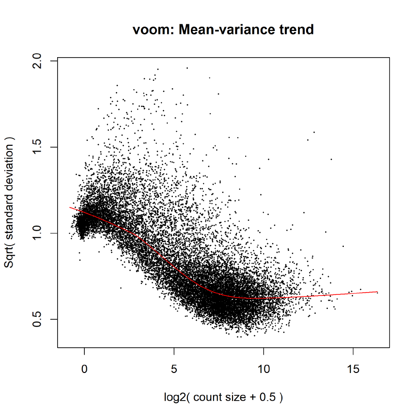
The intra cell line correlation will change the voom weights slightly, so we run voom a second
time:
> v <- voom(y, design, plot = TRUE, block = Targets$cellline, correlation = cor$consensus)
Similary, we run update the correlation for the new voom weights:
> cor <- duplicateCorrelation(v, design, block = Targets$cellline)
> cor$consensus
[1] 0.446
The correlation has hardly changed on the second iteration.
Now find genes differentially expression between male and females. Positive log-fold-changes
mean higher in males.
128
> fit <- lmFit(v, design, block = Targets$cellline, correlation = cor$consensus)
> fit <- eBayes(fit)
> summary(decideTests(fit))
(Intercept) genderMale concentration2.5 concentration3.5
Down 1464 27 1469 4105
NotSig 3352 16869 13622 9704
Up 12102 22 1827 3109
> topTable(fit, coef = "genderMale", n = Inf, sort = "p", p = 0.05)[,-1]
Chr Length Symbol type_of_gene logFC AveExpr t P.Value adj.P.Val B
64595 Y 5242 TTTY15 miscRNA 6.529 -0.258 52.97 3.63e-68 6.14e-64 123.983
6192 Y 897 RPS4Y1 protein-coding 9.691 2.224 44.08 1.91e-61 1.62e-57 117.215
9086 Y 1390 EIF1AY protein-coding 7.962 0.659 42.44 4.52e-60 2.55e-56 113.661
8284 Y 5581 KDM5D protein-coding 7.148 2.566 41.47 3.08e-59 1.30e-55 115.802
8653 Y 4795 DDX3Y protein-coding 6.439 3.547 39.30 2.68e-57 9.08e-54 114.155
7503 X 19271 XIST miscRNA -10.223 4.135 -37.53 1.20e-55 3.37e-52 107.001
8287 Y 10040 USP9Y protein-coding 5.693 1.982 36.51 1.14e-54 2.75e-51 107.303
7404 Y 7055 UTY protein-coding 5.945 1.670 34.29 1.93e-52 4.08e-49 102.661
246126 Y 865 TXLNG2P pseudo 5.316 -0.209 32.57 1.25e-50 2.36e-47 96.469
22829 Y 6276 NLGN4Y protein-coding 6.454 -0.241 32.14 3.65e-50 6.18e-47 95.755
9383 X 37027 TSIX miscRNA -9.314 3.511 -32.02 4.99e-50 7.67e-47 96.703
7544 Y 5616 ZFY protein-coding 5.029 0.799 30.89 8.90e-49 1.25e-45 94.753
5616 Y 7217 PRKY pseudo 3.090 2.542 23.92 4.22e-40 5.50e-37 79.334
140032 Y 888 RPS4Y2 protein-coding 3.670 -1.476 19.07 6.85e-33 8.28e-30 60.881
8226 X 2447 HDHD1 protein-coding -0.900 5.373 -10.09 2.59e-16 2.92e-13 26.572
8242 X 6862 KDM5C protein-coding -0.688 7.881 -9.70 1.59e-15 1.68e-12 24.728
100506003 Y 525 ZFY-AS1 miscRNA 1.689 -2.543 9.67 1.83e-15 1.82e-12 24.206
7403 X 5772 KDM6A protein-coding -0.689 5.044 -9.62 2.30e-15 2.16e-12 24.416
8228 X 2901 PNPLA4 protein-coding -0.889 3.901 -9.52 3.72e-15 3.31e-12 24.028
246119 Y 1628 TTTY10 miscRNA 1.793 -2.575 9.28 1.14e-14 9.66e-12 22.508
7543 X 7883 ZFX protein-coding -0.739 5.039 -8.56 3.52e-13 2.83e-10 19.434
6191 X 956 RPS4X protein-coding -0.857 10.630 -8.55 3.70e-13 2.85e-10 19.339
5613 X 6084 PRKX protein-coding -0.584 5.717 -8.04 4.07e-12 2.99e-09 16.967
1964 X 4431 EIF1AX protein-coding -0.699 4.679 -7.05 4.03e-10 2.84e-07 12.512
389906 X 1791 LOC389906 pseudo -0.701 3.021 -6.23 1.57e-08 1.06e-05 9.120
55787 X 4396 TXLNG protein-coding -0.442 5.405 -6.04 3.63e-08 2.36e-05 8.016
1654 X 5399 DDX3X protein-coding -0.573 7.960 -5.99 4.64e-08 2.91e-05 7.722
1968 X 3465 EIF2S3 protein-coding -0.570 7.845 -5.66 1.89e-07 1.14e-04 6.344
10943 X 4954 MSL3 protein-coding -0.721 6.933 -5.49 3.96e-07 2.31e-04 5.625
554203 X 1672 JPX miscRNA -0.739 1.572 -5.19 1.38e-06 7.78e-04 4.975
56999 3 7313 ADAMTS9 protein-coding 1.304 -2.386 5.04 2.45e-06 1.34e-03 4.576
2941 6 1341 GSTA4 protein-coding -1.453 -0.270 -4.88 4.76e-06 2.52e-03 3.918
4267 X|Y 2474 CD99 protein-coding 0.535 5.466 4.85 5.30e-06 2.72e-03 3.145
159013 X 4250 CXorf38 protein-coding -0.329 5.569 -4.69 1.00e-05 4.88e-03 2.523
286554 Y 3668 BCORP1 pseudo 1.370 -2.576 4.69 1.01e-05 4.88e-03 3.262
23136 18 4446 EPB41L3 protein-coding 2.276 -0.215 4.67 1.09e-05 5.13e-03 3.122
27334 X 1790 P2RY10 protein-coding -0.469 5.853 -4.64 1.24e-05 5.58e-03 2.308
8233 X 1512 ZRSR2 protein-coding -0.525 4.282 -4.63 1.25e-05 5.58e-03 2.443
139341 X 1170 FUNDC1 protein-coding -0.525 3.419 -4.57 1.57e-05 6.82e-03 2.359
100506661 X 1203 LOC100506661 miscRNA -0.695 0.751 -4.54 1.80e-05 7.61e-03 2.610
8935 7 3971 SKAP2 protein-coding 0.455 5.566 4.44 2.66e-05 1.10e-02 1.581
1237 3 1487 CCR8 protein-coding -1.393 1.085 -4.43 2.73e-05 1.10e-02 2.187
57502 X 5815 NLGN4X protein-coding 1.585 -1.307 4.35 3.73e-05 1.47e-02 2.022
3552 2 2928 IL1A protein-coding -1.439 1.379 -4.09 9.48e-05 3.65e-02 0.980
6399 X 2860 TRAPPC2 protein-coding -0.467 3.629 -4.08 9.76e-05 3.67e-02 0.575
129
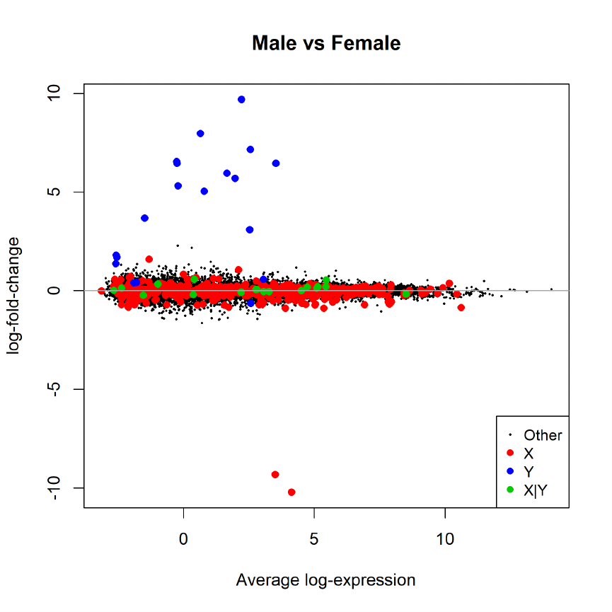
10333 4 5890 TLR6 protein-coding -0.473 4.510 -4.04 1.16e-04 4.27e-02 0.279
284486 1 1146 THEM5 protein-coding -1.074 0.264 -4.03 1.19e-04 4.30e-02 0.863
152273 3 5897 FGD5 protein-coding 1.033 -2.187 4.01 1.27e-04 4.49e-02 0.914
80086 2 1380 TUBA4B pseudo 0.833 1.659 4.00 1.32e-04 4.57e-02 0.602
As expected, the highly ranked genes are mostly on the X or Y chromosomes.
> chrom <- fit$genes$Chr
> plotMD(fit, column=2, status=chrom, values=c("X","Y", "X|Y"),
+ hl.col=c("red","blue", "green3"), main="Male vs Female",legend="bottomright")
> abline(h=0,col="darkgrey")
18.1.10 Gene set testing
Get the list of genes belonging to the male-specific region of chromosome Y [31], and a list of genes
located in the X chromosome that have been reported to escape X-inactivation [4]. The gender
130
genes are available at http://bioinf.wehi.edu.au/software/GenderGenes/. We expect genes in
the first list to be up-regulated in males, whereas genes in the second list should be up-regulated in
females.
> load(url("http://bioinf.wehi.edu.au/software/GenderGenes/GenderGenes.RData"))
> Ymale <- v$genes$GeneID %in% msYgenes
> Xescape <- v$genes$GeneID %in% XiEgenes
Roast gene set tests confirm that the male-specific genes are significantly up as a group in our
comparison of males with females, whereas the X genes are significantly down as a group [41]:
> index <- list(Y = Ymale, X = Xescape)
> mroast(v,index,design,2, block = Targets$cellline, correlation = cor$consensus, nrot=9999)
NGenes PropDown PropUp Direction PValue FDR PValue.Mixed FDR.Mixed
Y 13 0.000 1.0000 Up 1e-04 1e-04 1e-04 1e-04
X 54 0.574 0.0926 Down 1e-04 1e-04 1e-04 1e-04
The results from competitive camera gene sets tests are even more convincing [42]:
> camera(v,index,design,2)
NGenes Direction PValue FDR
Y 13 Up 2.40e-262 4.80e-262
X 54 Down 5.58e-26 5.58e-26
We can highlight the male-specific and X-escape genes on the mean-difference plot:
> status <- rep("Other",nrow(fit))
> status[Ymale] <- "Ymale"
> status[Xescape] <- "Xescape"
> plotMD(fit,column=2,status=status,values=c("Xescape","Ymale"),hl.col=c("blue","red"),
+ main="Male vs Female",legend="bottomright")
> abline(h=0,col="darkgrey")
131
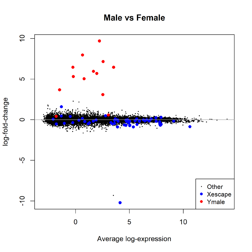
Another way to view the gene sets it to view the ranking of the Y and X specific genes in the
differential expression results. This shows that, with a couple of exceptions, the Y specific genes are
highly ranked (positive) while the X specific genes are low ranked (negative):
> barcodeplot(fit$t[,2],Ymale,Xescape, labels=c("Down in male","Up in male"))
> legend("top",legend=c("Ymale genes","Xescape genes"),lty=1,col=c("red","blue"))
132
Statistic
Down in male
Up in male
−37.53
−1.65
−1.11
−0.71
−0.37
−0.05
0.27
0.61
1.00
1.54
52.97
0 7.64.1 0
EnrichmentEnrichment
Ymale genes
Xescape genes
18.1.11 Session information
> sessionInfo()
R version 4.1.0 (2021-05-18)
Platform: x86_64-w64-mingw32/x64 (64-bit)
Running under: Windows 10 x64 (build 19042)
Matrix products: default
locale:
[1] LC_COLLATE=English_Australia.1252 LC_CTYPE=English_Australia.1252
[3] LC_MONETARY=English_Australia.1252 LC_NUMERIC=C
[5] LC_TIME=English_Australia.1252
attached base packages:
133
[1] stats graphics grDevices utils datasets methods base
other attached packages:
[1] edgeR_3.34.0 knitr_1.33 limma_3.49.1
loaded via a namespace (and not attached):
[1] compiler_4.1.0 magrittr_2.0.1 tools_4.1.0 Rcpp_1.0.7 stringi_1.6.2 highr_0.9
[7] grid_4.1.0 locfit_1.5-9.4 stringr_1.4.0 xfun_0.24 statmod_1.4.36 lattice_0.20-44
[13] evaluate_0.14
18.1.12 Acknowledgements
Thanks for Yang Liao for mapping the reads and running featureCounts.
18.2 Differential Splicing after Pasilla Knockdown
18.2.1 Background
This case study re-analyzes data produced by Brooks et al [2].
The proteins NOVA1 and NOVA2 are known to regulate splicing in mammals. Brooks et al used
Drosophila melanogaster as a model system, and used an RNA interference system (RNAi) to knock
down the expression of the D. melanogaster ortholog of NOVA1 and NOVA2, which is Pasilla (ps).
The experiment compared treated and untreated cells from the S2-DRSC cell line.
In this case study we find exons and genes that are differentially expressed after ps knockdown,
and we find genes are that are differentially spliced in the knockdown samples as compared to wild-
type.
For completeness, we will describe all the steps in the analysis from raw data files including
mapping and alignment. If you want to skip the mapping and read counting steps, go straight to
Section 18.2.6 where the statistical analysis begins.
18.2.2 GEO samples and SRA Files
Brooks et al [2] deposited data for six RNA samples to GEO http://www.ncbi.nlm.nih.gov/geo.
We have prepared the GEO accession numbers and titles in a csv file:
> library(limma)
> GEO <- readTargets("GEO-samples.csv", sep=",")
> GEO
GEO Title Pasilla
1 GSM461176 S2_DRSC_Untreated-1 Normal
2 GSM461177 S2_DRSC_Untreated-3 Normal
3 GSM461178 S2_DRSC_Untreated-4 Normal
4 GSM461179 S2_DRSC_CG8144_RNAi-1 Down
5 GSM461180 S2_DRSC_CG8144_RNAi-3 Down
6 GSM461181 S2_DRSC_CG8144_RNAi-4 Down
There are three untreated biological samples, in which ps should be expressed at normal levels, and
three treated biological samples, in which ps should be expressed at reduced levels.
134
While GEO records the sample information, the sequencing data file are actually held on the NCBI
Short Read Archive (SRA). The RNA samples were sequenced on an Illumina Genome Analyzer II.
Multiple sequencing runs were used for several of the samples, resulting in a total of 20 SRA files:
> SRA <- readTargets("SRA-Files.csv", sep=",")
> SRA
SRA GEO Title RunDate FlowCellID Type ReadLength
1 SRR031708 GSM461176 S2_DRSC_Untreated-1 7/15/08 308T2AAXX SE 45
2 SRR031709 GSM461176 S2_DRSC_Untreated-1 7/15/08 308T2AAXX SE 45
3 SRR031710 GSM461176 S2_DRSC_Untreated-1 8/15/08 30AYWAAXX SE 45
4 SRR031711 GSM461176 S2_DRSC_Untreated-1 8/15/08 30AYWAAXX SE 45
5 SRR031712 GSM461176 S2_DRSC_Untreated-1 8/15/08 30AYWAAXX SE 45
6 SRR031713 GSM461176 S2_DRSC_Untreated-1 8/15/08 30AYWAAXX SE 45
7 SRR031714 GSM461177 S2_DRSC_Untreated-3 11/14/08 30MNEAAXX PE 37
8 SRR031715 GSM461177 S2_DRSC_Untreated-3 12/23/08 30M2BAAXX PE 37
9 SRR031716 GSM461178 S2_DRSC_Untreated-4 12/23/08 30M2BAAXX PE 37
10 SRR031717 GSM461178 S2_DRSC_Untreated-4 12/23/08 30M2BAAXX PE 37
11 SRR031718 GSM461179 S2_DRSC_CG8144_RNAi-1 7/15/08 308T2AAXX SE 45
12 SRR031719 GSM461179 S2_DRSC_CG8144_RNAi-1 7/18/08 308UEAAXX SE 45
13 SRR031720 GSM461179 S2_DRSC_CG8144_RNAi-1 8/15/08 30AYWAAXX SE 45
14 SRR031721 GSM461179 S2_DRSC_CG8144_RNAi-1 8/15/08 30AYWAAXX SE 45
15 SRR031722 GSM461179 S2_DRSC_CG8144_RNAi-1 8/15/08 30AYWAAXX SE 45
16 SRR031723 GSM461179 S2_DRSC_CG8144_RNAi-1 8/21/08 308A0AAXX SE 45
17 SRR031724 GSM461180 S2_DRSC_CG8144_RNAi-3 12/23/08 30M2BAAXX PE 37
18 SRR031725 GSM461180 S2_DRSC_CG8144_RNAi-3 12/23/08 30M2BAAXX PE 37
19 SRR031726 GSM461181 S2_DRSC_CG8144_RNAi-4 12/23/08 30M2BAAXX PE 37
20 SRR031727 GSM461181 S2_DRSC_CG8144_RNAi-4 12/23/08 30M2BAAXX PE 37
Run dates are in American format, so that 7/15/08 denotes 15 July 2008. All runs in July and August
2008 used single end (SE) sequencing with 45 base-pair reads, while the later runs used paired end
(PE) sequencing with 37 bp reads.
18.2.3 Mapping reads to the reference genome
The reads were mapped to the reference D. melanogaster genome using Rsubread [15].
First the SRA format files need to be converted to FASTQ format, which is the de facto standard
for representing high-throughput sequencing data. The was done using the SRA Toolkit version 2.3.4.
Specifically the Unix SRA toolkit command fastq-dump --split-spot --split-files was used to
produce one FASTQ file for each single-end SRA file and two FASTQ files for each paired-end SRA
file.
Second, FASTA files representing the D. melanogaster genome were downloaded from ftp://ftp.
ncbi.nlm.nih.gov/genomes/Drosophila_melanogaster/RELEASE_5_48. There are five FASTA
files corresponding to chromosome arms:
> DM <- readTargets("FASTA-GFF-files.csv",sep=",")
> DM
FASTA GFF Chromosome
1 CHR_2/NT_033778.fna CHR_2/NT_033778.gff Chr2R
2 CHR_2/NT_033779.fna CHR_2/NT_033779.gff Chr2L
3 CHR_3/NT_033777.fna CHR_3/NT_033777.gff Chr3R
4 CHR_3/NT_037436.fna CHR_3/NT_037436.gff Chr3L
5 CHR_4/NC_004353.fna CHR_4/NC_004353.gff Chr4
6 CHR_X/NC_004354.fna CHR_X/NC_004354.gff ChrX
135

The five *.fna files were concatenated into a single FASTA-format file Drosophila ref.fasta, and an
index file was built using Rsubread
> library(Rsubread)
> buildindex(basename="index",reference="Drosophila_ref.fasta")
Third, reads were aligned to the genome. The SE reads were mapped using:
> align("index",SE_fastq_files,input_format="FASTQ")
where SE fastq files is a character vector containing the names of the SE FASTQ files. The PE
reads were mapped using:
> align("index",PE_fastq_files1,PE_fastq_files2,input_format="FASTQ")
where PE fastq files1 and PE fastq files2 are vectors containing the names of the PE FASTQ files.
These commands produce BAM files containing aligned reads (SE) or fragments (PE).
18.2.4 Read counts for exons
Next we counted the number of reads or fragments overlapping each annotated exon of each gene.
GFF files containing gene and exon annotation were downloaded from ftp://ftp.ncbi.nlm.nih.
gov/genomes/Drosophila_melanogaster/RELEASE_5_48. There is one GFF file for each chromo-
some arm as shown above.
The five *.gff files were concatenated into one file, and repeated exons instances of the same
exon (same start and stop position) were removed, to create a data.frame of start/stop positions
called unique.gff. SE reads were counted by:
> fc_SE <- featureCounts(SE_bam_files, annot.ext="unique.gff",
+ isGTFAnnotationFile=TRUE,
+ GTF.featureType="exon", GTF.attrType="ID",
+ useMetaFeatures=FALSE, allowMultiOverlap=TRUE)
where SE bam files is a vector of BAM file names for the SE reads. PE reads were counted by
> fc_PE <- featureCounts(PE_bam_files, annot.ext="unique.gff",
+ isGTFAnnotationFile=TRUE,
+ GTF.featureType="exon", GTF.attrType="ID",
+ useMetaFeatures=FALSE, allowMultiOverlap=TRUE,
+ isPairedEnd=TRUE)
where PE bam files is a vector of BAM file names for the PE reads.
18.2.5 Assemble DGEList and sum counts for technical replicates
We assemble all the counts into an edgeR DGEList object:
> library(edgeR)
> y.all <- DGEList(counts=cbind(fc_SE$counts,fc_PE$counts), genes=fc_SE$annotation)
> dim(y.all)
[1] 74184 20
> head(y.all$genes)
136
GeneID Chr Start End Strand Length
138088 30970 NC_004354.3 138094 139379 - 1286
138087 30970 NC_004354.3 139445 139611 - 167
138089 30970 NC_004354.3 139445 139889 - 445
138086 30970 NC_004354.3 139713 139889 - 177
138091 30971 NC_004354.3 140011 141629 + 1619
138092 30971 NC_004354.3 142415 144271 + 1857
The annotation includes Entrez ID and the length, chromosome and start and stop position of each
exon.
Resort back to original SRA order:
> y.all <- y.all[,SRA$SRA]
Then we collapse the data so that there is a single column for each GEO sample by summing the
counts over the technical replicates:
> y <- sumTechReps(y.all, ID=SRA$GEO)
> y$samples
group lib.size norm.factors
GSM461176 1 31007529 1
GSM461177 1 13040952 1
GSM461178 1 15030819 1
GSM461179 1 28143539 1
GSM461180 1 14901292 1
GSM461181 1 16264066 1
> colnames(y) <- c("N1","N3","N4","D1","D3","D4")
18.2.6 Gene annotation
Annotation for D. melanogaster genes was downloaded from ftp://ftp.ncbi.nlm.nih.gov/gene/
DATA/GENE_INFO/Invertebrates. We now add selected annotation columns to the DGEList object:
> ncbi.L1 <- readLines("Drosophila_melanogaster.gene_info", n = 1)
> ncbi.colname <- unlist(strsplit(substring(ncbi.L1, 10, 234), ’ ’))
> ncbi <- read.delim("Drosophila_melanogaster.gene_info",
+ skip=1, header=FALSE, stringsAsFactors=FALSE)
> colnames(ncbi) <- ncbi.colname
> m <- match(y$genes$GeneID, ncbi$GeneID)
> y$genes$Chr <- ncbi$chromosome[m]
> y$genes$Symbol <- ncbi$Symbol[m]
> y$genes$Strand <- NULL
> head(y$genes)
GeneID Chr Start End Length Symbol
138088 30970 X 138094 139379 1286 CG3038
138087 30970 X 139445 139611 167 CG3038
138089 30970 X 139445 139889 445 CG3038
138086 30970 X 139713 139889 177 CG3038
138091 30971 X 140011 141629 1619 G9a
138092 30971 X 142415 144271 1857 G9a
137
18.2.7 Filtering
Keep exons that have more than 1 cpm in at least 3 samples.
> isexpr <- rowSums(cpm(y) > 1) >=3
> y <- y[isexpr,,keep.lib.sizes=FALSE]
18.2.8 Scale normalization
Apply TMM normalization.
> y <- calcNormFactors(y)
> y$sample
group lib.size norm.factors
N1 1 30872843 0.955
N3 1 12962245 1.031
N4 1 14908555 0.976
D1 1 27989806 1.005
D3 1 14760887 1.022
D4 1 16172265 1.014
An MDS plot shows clear separation of the Pasilla down vs normal samples, but also a batch effect
associated with sequencing type and date:
> plotMDS(y)
138

−1.0 −0.5 0.0 0.5 1.0 1.5
−1.0 −0.5 0.0 0.5 1.0
Leading logFC dim 1
Leading logFC dim 2
N1
N3
N4
D1
D3
D4
18.2.9 Linear modelling
Create design matrix:
> Batch <- factor(c(1,3,4,1,3,4))
> Pasilla <- factor(GEO$Pasilla,levels=c("Normal","Down"))
> design <- model.matrix(~ Batch + Pasilla)
Apply voom to convert the read counts to log2-cpm with associated weights:
> v <- voom(y,design,plot=TRUE)
139
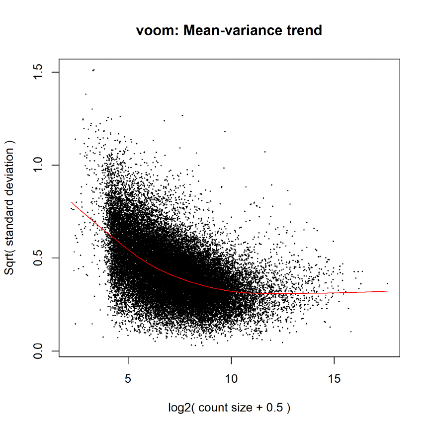
Linear modelling:
> fit <- lmFit(v, design)
Test for differentially expressed exons:
> fit.de <- eBayes(fit, robust=TRUE)
> topTable(fit.de, coef="PasillaDown")
GeneID Chr Start End Length Symbol logFC AveExpr t P.Value adj.P.Val B
150709 32007 X 10674926 10676128 1203 sesB -3.26 6.41 -32.1 4.45e-14 8.35e-10 22.3
150713 32007 X 10675026 10676128 1103 sesB -3.26 6.41 -32.1 4.48e-14 8.35e-10 22.3
96435 43230 3R 22694960 22695852 893 BM-40-SPARC -2.47 10.50 -28.2 2.51e-13 2.61e-09 20.9
150697 32008 X 10672987 10673728 742 Ant2 2.85 5.53 28.0 2.80e-13 2.61e-09 20.6
96434 43230 3R 22695915 22696094 180 BM-40-SPARC -2.27 8.11 -26.9 4.72e-13 3.52e-09 20.3
96433 43230 3R 22697648 22697717 70 BM-40-SPARC -2.17 6.27 -23.5 2.70e-12 1.46e-08 18.6
107856 44030 3L 2561932 2562843 912 msn -2.46 5.12 -23.5 2.80e-12 1.46e-08 18.5
140
70750 44258 3R 5271691 5272628 938 ps -2.27 5.53 -23.1 3.38e-12 1.46e-08 18.4
11333 44548 2R 6407125 6408782 1658 lola 2.25 5.73 23.1 3.54e-12 1.46e-08 18.3
150702 32008 X 10674230 10674694 465 Ant2 2.97 3.89 21.9 6.82e-12 2.34e-08 17.4
> summary(decideTests(fit.de))
(Intercept) Batch3 Batch4 PasillaDown
Down 443 5380 6070 2062
NotSig 3388 26386 25184 33346
Up 33427 5492 6004 1850
18.2.10 Alternate splicing
Test for differences in exon retention between Pasilla down vs normal:
> ex <- diffSplice(fit[,"PasillaDown"], geneid = "GeneID", exonid = "Start")
Total number of exons: 37258
Total number of genes: 8192
Number of genes with 1 exon: 1619
Mean number of exons in a gene: 5
Max number of exons in a gene: 56
Show top genes that show differential splicing.
> topSplice(ex, test="simes", n=20)
GeneID Chr Symbol NExons P.Value FDR
11214 44548 2R lola 30 5.52e-32 3.63e-28
95956 44448 3R scrib 35 1.99e-20 4.41e-17
141235 45320 X trol 44 2.01e-20 4.41e-17
16060 36542 2R shot 38 5.12e-18 7.80e-15
107810 44030 3L msn 24 5.93e-18 7.80e-15
19880 36773 2R Dg 15 5.15e-17 5.64e-14
32242 37893 2R slik 19 1.93e-16 1.81e-13
41795 3771968 2L Msp-300 33 2.27e-16 1.86e-13
82117 42130 3R osa 17 1.14e-15 8.34e-13
150694 32008 X Ant2 5 6.26e-14 4.12e-11
52823 34652 2L vir-1 7 4.62e-13 2.76e-10
115767 38879 3L pbl 12 7.60e-13 4.16e-10
163416 32817 X CrebB-17A 12 1.22e-11 6.16e-09
110493 38491 3L ens 16 2.31e-11 1.08e-08
2032 2768716 2R mim 25 1.51e-10 6.60e-08
166094 33098 X CG32521 8 1.63e-10 6.69e-08
131170 40205 3L CG42674 16 2.16e-10 8.36e-08
109416 38418 3L kst 18 3.92e-10 1.43e-07
150710 32007 X sesB 7 1.06e-09 3.49e-07
526 35494 2R laccase2 9 1.08e-09 3.49e-07
> topSplice(ex, test="F", n=20)
GeneID Chr Symbol NExons F P.Value FDR
141235 45320 X trol 44 30.87 1.93e-40 1.27e-36
11214 44548 2R lola 30 41.80 4.81e-33 1.58e-29
95956 44448 3R scrib 35 16.20 1.53e-23 3.35e-20
141
41795 3771968 2L Msp-300 33 13.81 2.66e-20 4.37e-17
32242 37893 2R slik 19 26.39 1.91e-18 2.52e-15
16060 36542 2R shot 38 9.43 1.51e-17 1.65e-14
166094 33098 X CG32521 8 65.84 3.26e-14 3.06e-11
19880 36773 2R Dg 15 18.78 6.19e-13 5.08e-10
150694 32008 X Ant2 5 119.76 8.01e-13 5.85e-10
2032 2768716 2R mim 25 9.55 1.42e-12 9.32e-10
107810 44030 3L msn 24 9.91 1.68e-12 1.00e-09
82117 42130 3R osa 17 12.87 2.03e-11 1.11e-08
52823 34652 2L vir-1 7 44.35 2.92e-11 1.43e-08
150710 32007 X sesB 7 44.17 3.05e-11 1.43e-08
115767 38879 3L pbl 12 15.22 8.55e-10 3.75e-07
163416 32817 X CrebB-17A 12 14.92 1.10e-09 4.52e-07
134207 40464 3L Ten-m 12 13.79 2.99e-09 1.16e-06
108973 38376 3L BtbVII 10 16.87 3.81e-09 1.39e-06
11103 36104 2R G-oalpha47A 13 11.96 5.66e-09 1.96e-06
139657 44505 X br 13 11.50 9.41e-09 3.09e-06
We can plot all the exons for the most differentially spliced genes:
> plotSplice(ex, geneid="lola", genecol="Symbol")
●
●
●
●
●
●
●
●
●
●
●
●
●
●
●
●
●
●
●
●
●
●
●
●
●
●
●
●
●
●
−2 −1 0 1 2
lola
logFC (this exon vs rest)
6369712
6374902
6377019
6377677
6378765
6383800
6387703
6392364
6394928
6397300
6398030
6402519
6403340
6405418
6406208
6407125
6409533
6409533
6411002
6412310
6414072
6414571
6419253
6419544
6419686
6420623
6421081
6422355
6428850
6430410
Exon Start
●
●
●
●
●
●
●
●
●
●
●
●
This plot highlights exons that are individually significant in that they have fold changes larger or
smaller than most other exons.
142
> plotSplice(ex, geneid="scrib", genecol="Symbol")
●
●
●
●
●
●
●
●
●
●
●
●
●
●
●
●
●
●
●
●
●
●
●
●
●
●
●
●
●
●
●
●
●
●
●
−2.0 −1.0 0.0 0.5 1.0
scrib
logFC (this exon vs rest)
22362072
22362072
22362072
22363093
22370765
22380079
22380955
22392083
22392646
22393010
22393199
22399576
22400302
22400573
22400887
22402079
22402079
22404443
22404824
22405366
22405611
22405900
22406055
22406418
22406418
22410022
22415630
22416163
22420498
22420498
22423369
22424299
22426969
22426969
22429282
Exon Start
●
●
●
●
●
●
●
●
> plotSplice(ex, geneid="trol", genecol="Symbol")
143
●
●
●
●
●
●
●
●
●
●●
●
●
●
●
●
●
●
●
●
●
●
●
●
●
●
●
●
●
●
●
●
●
●
●
●
●
●
●
●
●
●
●
●
0 2 4 6
trol
logFC (this exon vs rest)
2364493
2365041
2366985
2367208
2367693
2368463
2369449
2369857
2374609
2374767
2375103
2375450
2376030
2376492
2377157
2377519
2378366
2378650
2380090
2380960
2382114
2384489
2385352
2385514
2386379
2386688
2387021
2388437
2389074
2389981
2390494
2390809
2391351
2392055
2392516
2393244
2395660
2407676
2415567
2416257
2417438
2417672
2417919
2438498
Exon Start
●
●
●
●
●
●
●
●
●
●
●
●
●
●
●
●
●
We can see that a block of five or six exons at the right end of the trol gene are relatively lost when
Pasilla is down, at the expense of an earlier block of twelve exons which become relatively more
highly expressed when Pasilla is down. Most exons in the first half of the gene behave similarly to
each other. This gene is on the negative strand, so transcription is from right to left. Thus figure
can be compared to Supplementary Figure 8A in Brooks et al [2]. The gene trol was identified by
Brooks et al to have a novel set of coordinately regulated exons. Brooks et al said:
“A particularly striking example involving these unannotated splice junctions is found in
the trol gene in which a group of nine contiguous exons, which are annotated as being
constitutive, are coordinately skipped in untreated cells . . . but coordinately included in
the ps(RNAi) cells . . .”
18.2.11 Session information
> sessionInfo()
R version 3.6.1 (2019-07-05)
Platform: x86_64-w64-mingw32/x64 (64-bit)
Running under: Windows 10 x64 (build 15063)
Matrix products: default
144
locale:
[1] LC_COLLATE=English_Australia.1252 LC_CTYPE=English_Australia.1252
[3] LC_MONETARY=English_Australia.1252 LC_NUMERIC=C
[5] LC_TIME=English_Australia.1252
attached base packages:
[1] stats graphics grDevices utils datasets methods base
other attached packages:
[1] edgeR_3.27.13 limma_3.41.15
loaded via a namespace (and not attached):
[1] compiler_3.6.1 tools_3.6.1 Rcpp_1.0.2 grid_3.6.1 locfit_1.5-9.1 statmod_1.4.32
[7] lattice_0.20-38
18.2.12 Acknowledgements
Thanks for Yang Liao for mapping the reads and running featureCounts.
145
Notes
Acknowledgements
Thanks to Jean Yee Hwa Yang and Sandrine Dudoit for the first three data sets. The Swirl zebrafish
data were provided by Katrin Wuennenburg-Stapleton from the Ngai Lab at UC Berkeley. Laurent
Gautier made the ecoliLeucine data set available on Bioconductor. Lynn Corcoran provided the
Bob1 Mutant data. Andrew Holloway, Ryan van Laar and Dileepa Diyagama provided the quality
control data set. Marnie Blewitt and Natasha Jansz provided the Smchd1 RNA-seq data.
Many current and former members of the Smyth Lab (students, programmers, postdocs) have
contributed to the development of particular functions in limma as acknowledged in the limma package
description and on the function help pages.
The limma package has benefited from many people who have made suggestions or reported bugs
including Kemal Akat, Naomi Altman, Gioia Altobelli, James Arnold, Alain Bateman, Ido Ben-Zvi,
Henrik Bengtsson, Lourdes Pe˜na Castillo, Dongseok Choi, Marcus Davy, Simon de Bernard, Ramon
Diaz-Uriarte, Lars Eijssen, P¨ar Engstr¨om, Egil Ferkingstad, Anthoula Gaigneaux, Robert Gentle-
man, Guido Hooiveld, Wolfgang Huber, Derek Janszen, William Kenworthy, Axel Klenk, Kevin Koh,
Erik Kristiansson, Mette Langaas, Michael Lawrence, Gildas Le Corguille, Gregory Lefebvre, Philip
Lijnzaad, Andrew Lynch, James MacDonald, Martin Maechler, Aaron Mackey, Steffen Moeller,
Duarte Molha, Florian Nigsch, Ashley Ng, Mario Novkovic, Ron Ophir, Francois Pepin, Sergi Sayols
Puig, Hubert Rehrauer, Davide Risso, Mark Robinson, Ken Simpson, Dario Strbenac, Laurentiu Adi
Tarca, Dan Tenenbaum, Gregory Theiler, Ryan C. Thompson, Joern Toedling, Michael Turewicz,
Bj¨orn Usadel, Chris Wilkinson, Beth Wilmot, Jean Yee Hwa Yang, John Zhang.
Conventions
Where possible, limma tries to use the convention that class names are in upper CamelCase, i.e., the
first letter of each word is capitalized, while function names are in lower camelCase, i.e., first word
is lowercase. When periods appear in function names, the first word should be an action while the
second word is the name of a type of object on which the function acts.
Software Projects Using limma
The limma package is used as a building block or as the underlying computational engine by many
software projects designed to provide user-interfaces for microarray or RNA-seq data analysis.
146
Bibliography
1. Benjamini, Y. and Hochberg, Y. (1995). Controlling the false discovery rate: a practical and
powerful approach to multiple testing. Journal of the Royal Statistical Society Series B 57,
289–300.
2. Brooks, A.N., Yang, L., Duff, M.O., Hansen, K.D., Park, J.W., Dudoit, S., Brenner, S.E.,
and Graveley, B.R. (2011). Conservation of an RNA regulatory map between Drosophila and
mammals. Genome Res 21, 193–202.
3. Callow, M.J., Dudoit, S., Gong, E.L., Speed, T.P., and Rubin, E.M. (2000). Microarray expres-
sion profiling identifies genes with altered expression in HDL deficient mice. Genome Research
10, 2022–2029.
4. Carrel, L. and Willard, H.F. (2005). X-inactivation profile reveals extensive variability in X-
linked gene expression in females. Nature 434, 400–404.
5. Chen, Y., Lun, A.T.L., and Smyth, G.K. (2016). From reads to genes to pathways: differential
expression analysis of RNA-seq experiments using Rsubread and the edgeR quasi-likelihood
pipeline. F1000Research 5, 1438.
6. Dalgaard, P. (2002). Introductory Statistics with R. Springer, New York.
7. Diaz, E., Ge, Y., Yang, Y.H., Loh, K.C., Serafini, T.A., Okazaki, Y., Hayashizaki, Y., Speed, T.,
P., Ngai, J., and Scheiffele, P. (2002). Molecular analysis of gene expression in the developing
pontocerebellar projection system. Neuron 36, 417–434.
8. Ellis, L., Pan, Y., Smyth, G., George, D., McCormack, C., Williams-Truax, R., Mita, M., Beck,
J., Burris, H., Ryan, G., et al. (2008). Histone deacetylase inhibitor panobinostat induces clinical
responses with associated alterations in gene expression profiles in cutaneous T-cell lymphoma.
Clinical Cancer Research 14, 4500–4510.
9. Hung, S., Baldi, P., and Hatfield, G.W. (2002). Global gene expression profiling in Escherichia
coli K12: The effects of leucine-responsive regulatory protein. Journal of Biological Chemistry
277, 40309–40323.
10. International HapMap Consortium, T. (2005). A haplotype map of the human genome. Nature
437, 1299–1320.
11. Irizarry, R. (2005). From CEL files to annotated lists of interesting genes. In R. Gentleman,
V. Carey, S. Dudoit, R. Irizarry, and W. Huber, editors, Bioinformatics and Computational
Biology Solutions using R and Bioconductor, pages 431–442. Springer, New York.
147
12. Law, C.W., Alhamdoosh, M., Su, S., Smyth, G.K., and Ritchie, M.E. (2016). RNA-seq analysis
is easy as 1-2-3 with limma, Glimma and edgeR. F1000Research 5, 1408.
13. Law, C.W., Chen, Y., Shi, W., and Smyth, G.K. (2014). Voom: precision weights unlock linear
model analysis tools for RNA-seq read counts. Genome Biology 15, R29.
14. Li, B. and Dewey, C.N. (2011). RSEM: accurate transcript quantification from RNA-Seq data
with or without a reference genome. BMC Bioinformatics 12, 323.
15. Liao, Y., Smyth, G.K., and Shi, W. (2019). The R package Rsubread is easier, faster, cheaper
and better for alignment and quantification of RNA sequencing reads. Nucleic Acids Research
47, e47.
16. Lim, E., Vaillant, F., Wu, D., Forrest, N., Pal, B., Hart, A., Asselin-Labat, M., Gyorki, D., Ward,
T., Partanen, A., et al. (2009). Aberrant luminal progenitors as the candidate target population
for basal tumor development in BRCA1 mutation carriers. Nature Medicine 15, 907–913.
17. Liu, R., Holik, A.Z., Su, S., Jansz, N., Chen, K., Leong, H.S., Blewitt, M.E., Asselin-Labat,
M.L., Smyth, G.K., and Ritchie, M.E. (2015). Why weight? modelling sample and observational
level variability improves power in RNA-seq analyses. Nucleic Acids Research 43, e97.
18. Milliken, G.A. and Johnson, D.E. (1992). Analysis of Messy Data, Volume 1: Designed Experi-
ments. Chapman & Hall, New York.
19. Oshlack, A., Emslie, D., Corcoran, L., and Smyth, G. (2007). Normalization of boutique two-
color microarrays with a high proportion of differentially expressed probes. Genome Biology 8,
R2.
20. Peart, M., Smyth, G., Van Laar, R., Bowtell, D., Richon, V., Marks, P., Holloway, A., and
Johnstone, R. (2005). Identification and functional significance of genes regulated by structurally
different histone deacetylase inhibitors. Proceedings of the National Academy of Sciences of the
United States of America 102, 3697–3702.
21. Phipson, B., Lee, S., Majewski, I.J., Alexander, W.S., and Smyth, G.K. (2016). Robust hyperpa-
rameter estimation protects against hypervariable genes and improves power to detect differential
expression. Annals of Applied Statistics 10, 946–963.
22. Pickrell, J.K., Marioni, J.C., Pai, A.A., Degner, J.F., Engelhardt, B.E., Nkadori, E., Veyrieras,
J.B., Stephens, M., Gilad, Y., and Pritchard, J.K. (2010). Understanding mechanisms underlying
human gene expression variation with RNA sequencing. Nature 464, 768–772.
23. Pickrell, J.K., Pai, A.A., Gilad, Y., and Pritchard, J.K. (2010). Noisy splicing drives mRNA
isoform diversity in human cells. PLoS Genetics 6, e1001236.
24. Reiner, A., Yekutieli, D., and Benjamini, Y. (2003). Identifying differentially expressed genes
using false discovery rate controlling procedures. Bioinformatics 19, 368–375.
25. Ritchie, M., Diyagama, D., Neilson, J., Van Laar, R., Dobrovic, A., Holloway, A., and Smyth, G.
(2006). Empirical array quality weights in the analysis of microarray data. BMC bioinformatics
7, 261.
148
26. Ritchie, M., Silver, J., Oshlack, A., Holmes, M., Diyagama, D., Holloway, A., and Smyth, G.
(2007). A comparison of background correction methods for two-colour microarrays. Bioinfor-
matics 23, 2700–2707.
27. Ritchie, M.E., Phipson, B., Wu, D., Hu, Y., Law, C.W., Shi, W., and Smyth, G.K. (2015). limma
powers differential expression analyses for RNA-sequencing and microarray studies. Nucleic Acids
Research 43, e47.
28. Robinson, M.D. and Oshlack, A. (2010). A scaling normalization method for differential expres-
sion analysis of RNA-seq data. Genome Biology 11, R25.
29. Shi, W., De Graaf, C., Kinkel, S., Achtman, A., Baldwin, T., Schofield, L., Scott, H., Hilton, D.,
and Smyth, G. (2010). Estimating the proportion of microarray probes expressed in an RNA
sample. Nucleic Acids Research 38, 2168–2176.
30. Shi, W., Oshlack, A., and Smyth, G. (2010). Optimizing the noise versus bias trade-off for
Illumina Whole Genome Expression Beadchips. Nucleic Acids Research 38, e204.
31. Skaletsky, H., Kuroda-Kawaguchi, T., Minx, P.J., Cordum, H.S., Hillier, L., Brown, L.G., Rep-
ping, S., Pyntikova, T., Ali, J., Bieri, T., Chinwalla, A., Delehaunty, A., Delehaunty, K., Du,
H., Fewell, G., Fulton, L., Fulton, R., Graves, T., Hou, S.F., Latrielle, P., Leonard, S., Mardis,
E., Maupin, R., McPherson, J., Miner, T., Nash, W., Nguyen, C., Ozersky, P., Pepin, K., Rock,
S., Rohlfing, T., Scott, K., Schultz, B., Strong, C., Tin-Wollam, A., Yang, S.P., Waterston,
R.H., Wilson, R.K., Rozen, S., and Page, D.C. (2003). The male-specific region of the human Y
chromosome is a mosaic of discrete sequence classes. Nature 423, 825–837.
32. Smyth, G., Michaud, J., and Scott, H. (2005). Use of within-array replicate spots for assessing
differential expression in microarray experiments. Bioinformatics 21, 2067–2075.
33. Smyth, G. and Speed, T. (2003). Normalization of cDNA microarray data. Methods 31, 265–273.
34. Smyth, G., Yang, Y., and Speed, T. (2003). Statistical issues in cDNA microarray data analysis.
Methods in Molecular Biology 224, 111–136.
35. Smyth, G.K. (2004). Linear models and empirical Bayes methods for assessing differential ex-
pression in microarray experiments. Statistical Applications in Genetics and Molecular Biology
3, Article 3.
36. Smyth, G.K. and Altman, N.S. (2013). Separate-channel analysis of two-channel microarrays:
recovering inter-spot information. BMC Bioinformatics 14, 165.
37. Visvader, J.E. (2009). Keeping abreast of the mammary epithelial hierarchy and breast tumori-
genesis. Genes & development 23, 2563–2577.
38. Wettenhall, J.M., Simpson, K.M., Satterley, K., and Smyth, G.K. (2006). affylmGUI: a graphical
user interface for linear modeling of single channel microarray data. Bioinformatics 22, 897–899.
39. Wettenhall, J.M. and Smyth, G.K. (2004). limmaGUI: a graphical user interface for linear
modeling of microarray data. Bioinformatics 20, 3705–3706.
149
40. Wolfinger, R.D., Gibson, G., Wolfinger, E.D., Bennett, L., Hamadeh, H., Bushel, P., Afshari, C.,
and Paules, R.S. (2001). Assessing gene significance from cDNA microarray expression data via
mixed models. Journal of Computational Biology 8, 625–637.
41. Wu, D., Lim, E., Vaillant, F., Asselin-Labat, M., Visvader, J., and Smyth, G. (2010). ROAST:
rotation gene set tests for complex microarray experiments. Bioinformatics 26, 2176–2182.
42. Wu, D. and Smyth, G. (2012). Camera: a competitive gene set test accounting for inter-gene
correlation. Nucleic Acids Research 40, e133.
43. Yang, Y.H., Dudoit, S., Luu, P., Lin, D.M., Peng, V., Ngai, J., and Speed, T.P. (2002). Normal-
ization for cDNA microarray data: a robust composite method addressing single and multiple
slide systematic variation. Nucleic Acids Research 30, e15.
44. Yang, Y.H., Dudoit, S., Luu, P., and Speed, T.P. (2001). Normalization for cDNA microarray
data. In M.L. Bittner, Y. Chen, A.N. Dorsel, and E.R. Dougherty, editors, Microarrays: Optical
Technologies and Informatics, pages 141–152. Proceedings of SPIE, Volume 4266, San Jose, CA.
45. Yang, Y.H. and Speed, T.P. (2003). Design and analysis of comparative microarray experiments.
In T.P. Speed, editor, Statistical Analysis of Gene Expression Microarray Data, pages 35–91.
Chapman & Hall/CRC Press.
46. Yang, Y.H. and Thorne, N.P. (2003). Normalization for two-color cDNA microarray data. In
D.R. Goldstein, editor, Science and Statistics: A Festschrift for Terry Speed, pages 403–418.
Institute of Mathematical Statistics Lecture Notes – Monograph Series, Volume 40.
150
