
521
[ Journal of Labor Economics, 2006, vol. 24, no. 3]
䉷 2006 by The University of Chicago. All rights reserved.
0734-306X/2006/2403-0005$10.00
Evaluating the Differential Effects of
Alternative Welfare-to-Work Training
Components: A Reanalysis of the
California GAIN Program
V. Joseph Hotz, University of California, Los Angeles
Guido W. Imbens, University of California, Berkeley
Jacob A. Klerman, RAND
We show how data from an evaluation in which subjects are randomly
assigned to some treatment versus a control group can be combined
with nonexperimental methods to estimate the differential effects of
alternative treatments. We propose tests for the validity of these meth-
ods. We use these methods and tests to analyze the differential effects
of labor force attachment (LFA) versus human capital development
(HCD) training components with data from California’s Greater Av-
enues to Independence (GAIN) program. While LFA is more effec-
tive than HCD training in the short term, we find that HCD is
relatively more effective in the longer term.
I. Introduction
In this article, we explore ways of combining experimental data and
nonexperimental methods to estimate the differential effects of compo-
nents of training programs. In particular, we show how data from a multi-
We wish to thank Julie Mortimer, Wes Hartmann, and especially Oscar Mitnik
for their able research assistance on this project. Jan Hanley, Laurie McDonald,
and Debbie Wesley of RAND helped with the preparation of the data. We also

522 Hotz et al.
site experimental evaluation in which subjects are randomly assigned to
any treatment versus a control group that receives no treatment can be
combined with nonexperimental regression-adjustment methods to esti-
mate the differential effects of particular types of treatments. Our methods
allow the implemented programs to vary across sites and across subjects
within a site. The availability of such experimental data allows us to test,
in part, the plausibility of our regression-adjustment methods for elimi-
nating selection biases that result from nonrandom assignment of program
components to individuals in the various sites. We use our method to
adjust for across-site differences in background and preprogram variables
as well as postrandomization local economic conditions and validate our
methods on experimentally generated control groups in the spirit of the
approaches taken in LaLonde (1986), Heckman and Hotz (1989), Fried-
lander and Robins (1995) and in Heckman, Ichimura, and Todd (1997,
1998), Heckman, Ichimura, Smith, and Todd (1998), Dehejia and Wahba
(1999), and Hotz, Imbens, and Mortimer (2005).
We apply these methods and tests to reexamine the conclusions about
the relative effectiveness of alternative strategies for designing welfare-to-
work training programs. Over the last 3 decades, as the United States has
sought to reform its welfare system, states have sought to design their
mandated welfare-to-work programs in order to reduce dependency on
welfare and promote work among disadvantaged households. Over this
period, states differed in the components, or approach, they emphasized
in these programs.
One approach, the human capital development (HCD) approach, em-
phasizes education and vocational training programs, such as General
Equivalency Diploma (GED) and English as Second Language (ESL)
programs and vocational training in the health care industry. The HCD
approach seeks to improve the basic and job-related skills of welfare
recipients. Advocates of this approach argue that acquiring such skills is
necessary for adults on welfare to “get a job, especially one that is rela-
wish to thank Howard Bloom, Jim Riccio, Hans Bos, John Wallace, David Ell-
wood, and participants in the Institute for Research on Poverty and NBER sum-
mer institutes, workshops at Berkeley and UCLA, and the Tenth International
Conference on Panel Data for helpful comments on an earlier draft of this article
and also two referees who provided valuable comments and suggestions on an
earlier draft of this article. This research was funded, in part, by NSF Grant SES
9818644. Development of the methodological approaches used in this research
also was funded by a contract from the California Department of Social Services
to the RAND Corporation for the conduct of the Statewide CalWORKs Eval-
uation. All opinions expressed in this article and any remaining errors are solely
our responsibility. In particular, this article does not necessarily represent the
position of the National Science Foundation, the State of California or its agencies,
RAND, or the RAND Statewide CalWORKs Evaluation. Contact the corre-

Impacts of the GAIN Program 523
tively stable, pays enough to support their children and leaves them less
vulnerable during an economic downturn” (Gueron and Hamilton 2002,
1).
The other primary approach used in designing welfare-to-work pro-
grams is labor force attachment (LFA), such as job clubs, which teaches
welfare recipients how to prepare re´sume´s and interview for jobs and
provides assistance in finding jobs. The LFA approach seeks to move
adults on welfare quickly into jobs, even if they are low-paying jobs.
Supporters of the LFA approach “see work as the most direct route to
ending ...thenegative effects of welfare on families and children”
(Gueron and Hamilton 2002, 2). The advocates of the LFA approach also
argue that it is better than the formal classroom training stressed in the
HCD approach to build the skills of most low-skilled adults. A natural
question is, Which approach is better?
The MDRC Greater Avenues to Independence (GAIN) Evaluation was
one of the most influential evaluations that shed light on the impacts of
these two approaches. Welfare recipients in six California counties were
randomly assigned either to a treatment group that was to receive services
in a county based and designed welfare-to-work program or to a control
group to which these services were denied. Under the GAIN program,
California’s counties had considerable discretion designing their welfare-
to-work programs, and counties emphasized the LFA versus HDC ap-
proaches to different degrees. Thus, the MDRC study conducted separate
evaluations of each county’s program, where the training components of
the program, the populations served, and the prevailing local economic
conditions varied across counties.
To date, the results of this experimental evaluation often have been
interpreted as favoring the LFA relative to the HCD approach. Based on
an analysis of data, 3 years after random assignment, MDRC found that
the largest effects on participants were for Riverside County’s GAIN
program, a program that emphasized the LFA approach.
1
In contrast, the
GAIN participants in the three largest of the other counties in the MDRC
Evaluation (Alameda, Los Angeles, and San Diego counties), which placed
1
Among female heads of households on Aid to Families with Dependent Chil-
dren (AFDC) in Riverside’s GAIN program, the number of quarters in which
recipients worked was 63% higher than those for the control group, and trainees’
labor market earnings were 63% higher over the 3-year evaluation period. Riv-
erside County’s GAIN program emphasized the LFA approach with tightly fo-
cused job search assistance as well as providing participants with the consistent
message “that employment is central and should be sought expeditiously and that
opportunities to obtain low-paying jobs should not be turned down” (Hogan
1995, 5).

524 Hotz et al.
much greater emphasis on HDC, had much smaller gains.
2
The LFA, or
“work-first,” approach of Riverside received national (and international)
acclaim for its success
3
and has become the model for welfare-to-work
programs across the nation.
4
The fallacy of this conclusion stems from attributing all of the differ-
ences in results across counties to differences in the treatment approaches
used. For example, treatment effects could vary across programs due to
differences in the populations treated, in the strategies used to assign
various treatment components across that population, and to differences
in the economic environments and local labor market conditions.
5
While
MDRC made clear in its reports that its experimental design did not allow
one to directly draw inferences about the differential impact of alternative
types of welfare-to-work components such as LFA and HCD, the results
have been consistently interpreted by policy makers in exactly that way.
Thus, the second objective of this article is to use our methods to address
directly whether LFA worked better than HCD based on data for subjects
in the MDRC GAIN evaluation.
A third objective of our article is to distinguish the short-run from the
long-run effects of LFA versus HCD training components. The formal
MDRC GAIN evaluation was based on experimental estimates of pro-
gram impacts for a 3-year postrandomization period.
6
Extrapolating from
such short-run estimates of social program impacts to what will happen
in the longer run can be misleading, as Couch (1992) and Friedlander and
Burtless (1995) have noted. This is especially true for assessing the effec-
tiveness of HCD relative to LFA training approaches, since HCD training
components tend to be more time-intensive treatments and typically take
longer to complete relative to LFA programs. As such, there is a strong
presumption that results from short-term evaluations will tend to favor
work-first programs over human-capital development ones.
7
Estimates of
2
These counties experienced only a 21% increase in quarters of work and a
23% increase in earnings relative to the outcomes for the control group members
in these counties.
3
For example, the Riverside GAIN program was awarded the Harvard Ken-
nedy School of Government’s Innovations in American Government Award in
1996.
4
For example, the State of California strongly encouraged all of the state’s
counties to adopt the Riverside LFA approach in its GAIN programs.
5
See Hotz, Imbens, and Mortimer (2005) for a systematic development and
treatment of this issue. Also see Bloom, Hill, and Riccio (2005).
6
An unpublished MDRC report presents estimates for the first 5 years after
randomization.
7
A similar point is made by Mincer (1974) in his model of schooling decisions.
Therein, Mincer notes that at early ages the earnings of individuals who choose
additional schooling will be lower than those who choose to go to work at early
ages, simply because attending school inhibits going to work, even if all alternative

Impacts of the GAIN Program 525
program effects over a longer postenrollment period are needed to fairly
assess the relative long-run benefits of these alternative welfare-to-work
strategies.
To address the above substantive concerns, we apply our methods to
estimate both short- and long-term differential effects of the LFA versus
HCD training components in a reanalysis of the data from the MDRC
evaluation of California’s GAIN program. We focus our analysis on four
of the six California counties (Alameda, Los Angeles, Riverside, and San
Diego) analyzed in the original GAIN evaluation
8
and estimate differential
effects for the post–random assignment employment, labor market earn-
ings, and welfare participation outcomes of participants in this evaluation.
We make use of data on these outcomes for a period of 9 years after
random assignment, data that were not previously available. We exploit
the data for the control groups in this evaluation to implement the tests
of some of the assumptions that justify the use of nonexperimental re-
gression-adjustment methods. Finally, we consider the extent to which
inferences about the temporal patterns of training effect estimates are
sensitive to postrandomization variation in local labor market conditions.
As we establish below, our reanalysis of the GAIN data leads to a sub-
stantively different set of conclusions about the relative effectiveness of
LFA versus HCD training components.
II. The GAIN Program and the MDRC GAIN Evaluation
The GAIN program began in California in 1986 and, in 1989, became
the state’s official welfare-to-work or Job Opportunities and Basic Skills
Training (JOBS) Program, authorized by the Family Support Act.
9
Except
for female heads with children under the age of 6, all adults on welfare
were required to register in their county-of-residence GAIN program.
10
activities yield the same present value of lifetime earnings. See also Ham and
LaLonde (1996).
8
We omit the two rural counties included in the original MDRC evaluation
(Butte and Tulare), because these rural economies are quite different from the
economies of the four urban counties.
9
The legislation that created the GAIN program represented a political com-
promise between two groups in the state’s legislature with different visions of
how to reform the welfare system. One group favored the “work-first” approach,
i.e., use of a relatively short-term program of mandatory job search, followed by
unpaid work experience for participants who did not find jobs. The other group
favored the “human capital” approach, i.e., a program providing a broader range
of services designed to develop the skills of welfare recipients. In crafting the
GAIN legislation, these two groups compromised on a program that contained
work-first as well as basic skills and education components in what became known
as the GAIN Program Model. See Riccio and Friedlander (1992) for a more
complete description of this model.
10
See Riccio et al. (1989) for a more complete description of the criteria for
mandated participation.

526 Hotz et al.
Each registrant was administered a screening test to measure a registrant’s
basic reading and math skills, with the same test being used in all counties.
Registrants with low test scores and those who did not have a high school
diploma or GED were deemed “in need of basic education” and targeted
to receive HCD training components, such as Adult Basic Education
(ABE) and/or English as a Second Language (ESL) courses. Those judged
not to be in need of basic education were to bypass these basic education
services and to move either into LFA, such as job search assistance, or
HCD, such as vocational or on-the-job training. Decisions about which
activities GAIN registrants received were under the control of county
GAIN administrators. In fact, the legislation that established the GAIN
program gave California’s 58 counties substantial discretion and flexibility
in designing their programs, including the types and mix of training com-
ponents they offered to GAIN registrants (see Riccio and Friedlander
1992, chap. 1).
MDRC conducted a randomized evaluation of the impacts and cost
effectiveness of the GAIN program in six research counties (Alameda,
Butte, Los Angeles, Riverside, San Diego, and Tulare). Beginning in 1988,
MDRC randomly assigned a subset of the GAIN registrants in these
counties either to an experimental group, which was eligible to receive
GAIN services and subject to its participation mandates, or to a control
group, which was ineligible for GAIN services but could seek (on their
own initiative) alternative services in their communities. Control group
members were embargoed from GAIN services until June 30, 1993, and
for 2 years after this date they were allowed, but not required, to par-
ticipate in GAIN. MDRC collected data on experimental and control
group members in the research counties, including background and de-
mographic characteristics and pre–random assignment employment, earn-
ings, and welfare utilization. Originally, MDRC gathered data on em-
ployment, earnings, and welfare utilization
11
for a 3-year postrandom-
ization period and reported on the findings for these outcomes in their
primary GAIN evaluation reports.
12
Descriptive statistics and sample sizes for the participants in the MDRC
evaluation in the four counties analyzed here (Alameda, Los Angeles,
Riverside, and San Diego) are provided in table 1. We focus on GAIN
registrants who were members of single-parent households on Aid to
Families with Dependent Children (AFDC)—which are referred to as the
AFDC family group or AFDC-FG households—at the time of random
11
Most of these data were obtained from state and county administrative data
systems.
12
See Riccio and Friedlander (1992) and Riccio et al. (1994). In an unpublished
paper, Freedman et al. (1996) present impact estimates for a 5-year postrandom-
ization period, based on additional outcomes data gathered from administrative
data sources.

Impacts of the GAIN Program 527
assignment.
13
Such households constitute over 80% of the AFDC caseload
in California and the nation, and almost all are female-headed.
14
As shown
at the bottom of table 1, in all but Alameda county, the counties assigned
a larger (and varying) fraction of cases to the experimental group. Finally,
we provide, in table 1, p-values for tests of the differences between ex-
perimental and control group means for the background variables. In most
cases, there are no statistically significant differences in these variables by
treatment status. The one exception is the year and quarter in which cases
were enrolled into the MDRC GAIN evaluation. In particular, there are
rather large and statistically significant differences in the proportions of
experimental and control cases enrolled by quarter in Los Angeles and
San Diego counties.
15
These were the result of changes in the rates of
randomization to the control status over the enrollment periods in these
counties as MDRC attempted to meet targeted numbers of control cases
in these counties.
Table 1 reveals notable differences in the demographic and prerandom-
ization characteristics of the cases enrolled in the GAIN registrants across
counties. These differences stem from two factors. First, the composition
of the AFDC caseloads varies across counties. Second, the strategies that
counties adopted for registering participants from their existing caseloads
into GAIN activities also varied. The GAIN programs in Riverside and
San Diego counties sought to register all welfare cases in GAIN, while
the programs in Alameda and Los Angeles counties focused on long-term
welfare recipients. For example, Alameda County, which began its GAIN
program in the third quarter of 1989, first registered its long-term cases
and then registered cases that had entered the AFDC caseload more re-
cently. The GAIN program in Los Angeles County initially registered
only those cases that had been on welfare for 3 consecutive years. The
consequences of these differences in selection criteria can be seen in table
1. In Alameda and Los Angeles, over 95% of the cases had been on welfare
a year prior to random assignment; in San Diego and Riverside, fewer
(for some cells much fewer) than 65% had been.
13
The samples we utilize for three of the four counties (Alameda, Riverside,
and San Diego counties) are slightly smaller than the original samples used by
MDRC because of our inability to find records for some sample members in
California’s Unemployment Insurance Base Wage system (administered by the
California Economic Development Department) or because we were missing in-
formation on the educational attainment of the sample member. The number of
cases lost in these three counties is very small, never larger than 1.1% of the total
sample, and does not differ by experimental status.
14
Descriptions and results for the much smaller group of two-parent households
on AFDC (AFDC-U cases) are given in the working paper version of the paper
(Hotz, Imbens, and Klerman 2000).
15
There are smaller discrepancies between fractions of experimentals and con-
trols by year and quarter in Riverside County.

528
Table 1
Background Characteristics and Prerandomization Histories of GAIN Evaluation Participants from AFDC Caseload
Variable
Alameda
Los Angeles Riverside San Diego
Mean SD p-Value Mean SD p-Value Mean SD p-Value Mean SD p-Value
Age 34.69 8.61 .034 38.52 8.43 .668 33.63 8.20 .431 33.80 8.59 .911
White .18 .38 .806 .12 .32 .621 .52 .50 .533 .43 .49 .263
Hispanic .08 .26 .045 .32 .47 .233 .27 .45 .937 .25 .44 .089
Black .70 .46 .562 .45 .50 .600 .16 .37 .323 .23 .42 .345
Other ethnic groups .04 .20 .400 .11 .31 .663 .05 .22 .700 .09 .29 .473
Female head .95 .22 .978 .94 .24 .043 .88 .33 .633 .84 .37 .349
Only one child .42 .49 .458 .33 .47 .743 .39 .49 .079 .43 .50 .530
More than one child .57 .50 .391 .67 .47 .976 .58 .49 .093 .53 .50 .621
Child 0–5 years .31 .46 .340 .10 .31 .353 .16 .37 .922 .13 .34 .778
Highest grade completed 11.18 2.52 .921 9.54 3.55 .548 10.68 2.53 .938 10.66 3.04 .373
In need of basic education .65 .48 .885 .81 .40 .982 .60 .49 .615 .56 .50 .362
Earnings 1 quarter before
random assignment $213 $851 .797 $221 $874 .454 $452 $1,404 .452 $588 $1,485 .270
Earnings 4 quarters before
random assignment $264 $1,018 .012 $216 $866 .405 $614 $1,603 .073 $808 $1,879 .747
Earnings 8 quarters before
random assignment $220 $1,005 .460 $181 $796 .473 $728 $1,840 .003 $827 $1,958 .301
Employed 1 quarter before
random assignment .14 .34 .531 .12 .33 .469 .22 .42 .664 .27 .44 .118
Employed 4 quarters be-
fore random assignment .14 .34 .000 .13 .33 .634 .25 .43 .976 .29 .45 .926
Employed 8 quarters be-
fore random assignment .13 .33 .896 .11 .32 .565 .27 .44 .044 .28 .45 .149
AFDC benefits 1 quarter
before random
assignment $1,907 $526 .331 $1,874 $663 .792 $1,190 $1,043 .499 $1,159 $903 .046

529
AFDC benefits 4 quarters
before random
assignment $1,822 $551 .317 $1,867 $662 .440 $995 $1,027 .663 $1,008 $928 .098
On AFDC 1 quarter be-
fore random assignment .98 .14 .692 .99 .10 .341 .77 .42 .837 .73 .44 .086
On AFDC 4 quarters be-
fore random assignment .96 .19 .982 .98 .14 .765 .63 .48 .973 .60 .49 .102
Proportion entered GAIN
in 1988:Q3 .11 .31 .085 .15 .36 .000
Proportion entered GAIN
in 1988:Q4 .18 .38 .073 .24 .43 .000
Proportion entered GAIN
in 1989:Q1 .17 .38 .631 .24 .42 .000
Proportion entered GAIN
in 1989:Q2 .17 .37 .299 .21 .41 .205
Proportion entered GAIN
in 1989:Q3 .26 .44 .944 .56 .50 .000 .13 .34 .699 .16 .37 .000
Proportion entered GAIN
in 1989:Q4 .21 .41 .767 .26 .44 .000 .13 .34 .746
Proportion entered GAIN
in 1990:Q1 .32 .47 .769 .18 .39 .244 .11 .31 .165
Proportion entered GAIN
in 1990:Q2 .21 .41 .578
Number of experimental
cases 597 2,995 4,405 6,978
Number of control cases 601 1,400 1,040 1,154
Total number of cases 1,198 4,395 5,445 8,132
Fraction of cases in experi-
mental group .498 .681 .809 .858
Note.—Earnings and AFDC benefits are deflated by Consumer Price Index; in 1999 dollars. The columns headed “Mean” contain means and those headed “SD” contain
standard deviations for the full sample (i.e., both experimental and control groups). The p-values are for a test of difference between experimental and control group means.
530 Hotz et al.
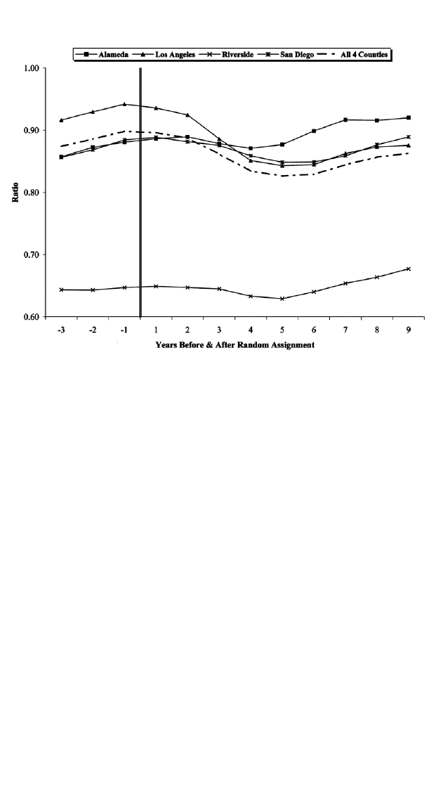
Fig. 1.—Annual ratio of total employment to adult population, all sectors
These differences in selection criteria also contributed to substantial
differences in the employment histories and individual characteristics of
the registrant populations across these four counties. As shown in table
1, the registrants in Alameda and Los Angeles counties had, on average,
much lower levels of earnings prior to random assignment relative to
those in Riverside and San Diego. Furthermore, the registrants in Alameda
and Los Angeles were, on average, older, had lower levels of educational
attainment, and were more likely to be assessed as “in need of basic
education” when they entered the GAIN program than the average reg-
istrants in Riverside and San Diego. The fact that Alameda and Los An-
geles counties focused on its “hard to treat” cases is a stark example of
how the caseload composition within the GAIN experiment varied across
counties and why it is implausible that all of the differences across counties
in treatment effects are due solely to the various treatment components.
The counties in the GAIN evaluation also differed with respect to the
conditions in the labor market immediately prior to random assignment,
and these differences also may account for the across-county differences
in the background characteristics and prerandomization outcomes of the
evaluation subjects displayed in table 1. Figures 1–4 display the time series
of two sets of measures of labor market conditions for each of the four
counties in the GAIN evaluation. Figure 1 plots the county-level ratio
of total employment to the adult population, and figure 2 displays the
Impacts of the GAIN Program 531
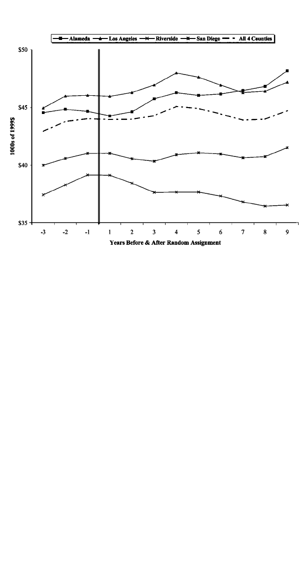
Fig. 2.—Annual earnings per worker, all sectors
average annual earnings per worker for those employed.
16
These measures
provide indicators of the across-county and over time differences in the
labor markets for the four counties in the years prior to random assign-
ment. Figures 3 and 4 display the corresponding employment-to-popu-
lation ratios and average annual earnings per work for those employed
in the retail trade sector, a sector of the economy in which many low-
skilled workers are employed.
17
In the periods prior to random assign-
ment, overall employment and employment in retail trade were increasing
in all four counties, although employment had begun to stagnate in many
of the counties. Furthermore, one notes substantial differences across the
four counties in these ratios, with Riverside county having a much lower
16
These county-level measures were constructed from data from the Regional
Economic Information System (REIS) maintained by the Bureau of Economic
Activity (BEA) in the U.S. Department of Commerce. We note that Hoynes (2000)
uses versions of both of these measures in her analysis of the effects of local labor
market conditions on welfare spells for the California AFDC caseload during the
late 1980s and early 1990s. See her paper for a discussion of these and other
county-level measures of local demand conditions.
17
Another sector of the economy that employs low-skilled workers is the ser-
vice sector. Based on measures comparable to those in figs. 3 and 4, similar trends
and differences across counties were found for this sector as those for the retail
trade sector.
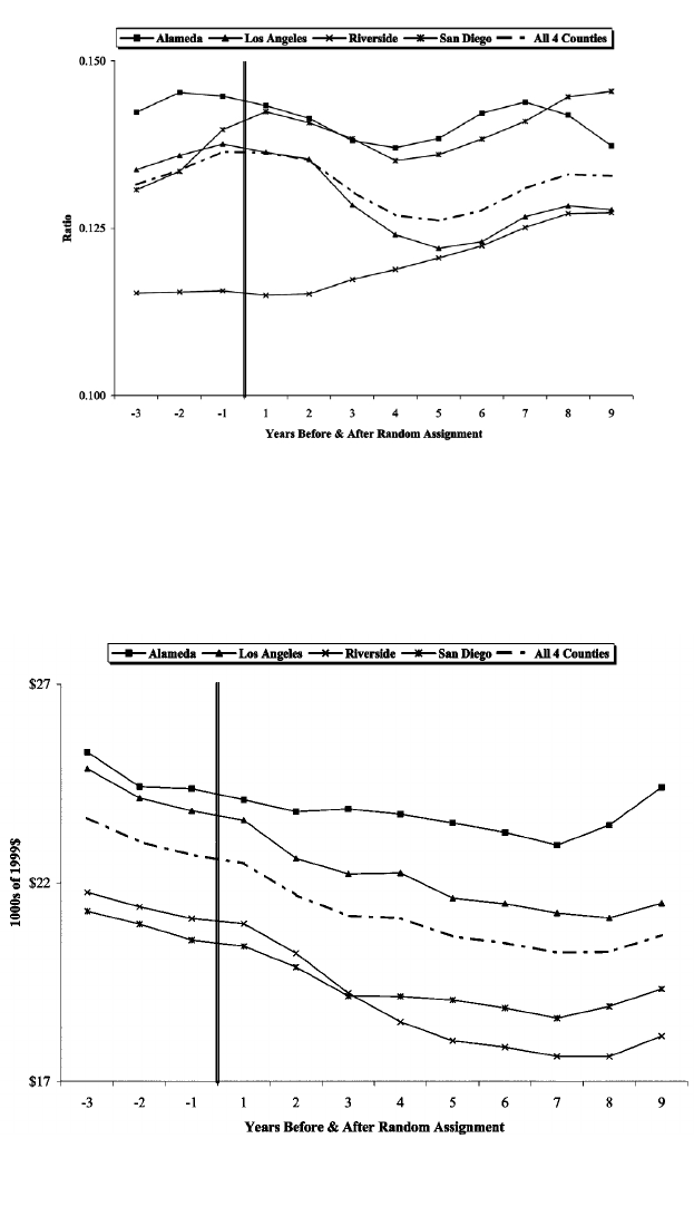
Fig. 3.—Ratio of annual employment in retail trade sector to adult population
Fig. 4.—Annual earnings per worker, retail trade sector

Impacts of the GAIN Program 533
total employment to adult population ratio than the other three counties.
18
Over this same period, average annual earnings per worker were increasing
in all but Alameda county (fig. 2), while earnings per worker in the retail
trade sector were declining (in real terms) in all four counties (fig. 4).
Moreover, one sees that overall earnings, as well as earnings in the retail
sector, were higher in Alameda and Los Angeles counties relative to Riv-
erside and San Diego counties. Toward the end of the next section, we
shall comment further on the postrandomization trends in these figures.
Finally, as we noted above, the four analysis counties in the GAIN
evaluation differed in the way they ran the programs and in the training
components they emphasized. In table 2, we display the proportions of
GAIN registrants in the four analysis counties that participated in various
training components during the period in which subjects were enrolled
in the MDRC GAIN evaluation.
19
One can see that Riverside county
placed fewer of its GAIN registrants in HCD training components than
did the administrators of the GAIN programs in the other three counties
during the period of enrollment in the MDRC evaluation. This is espe-
cially true relative to the proportions of GAIN registrants enrolled in the
MDRC evaluation that were deemed “in need of basic skills,” presumably
the group in greater need of HCD training components. (The proportions
of these groups, by year/quarter of enrollment into the MDRC evaluation,
are found in the last column of table 2.) As a crude indicator of the
relationship between HCD services relative to those registrants in need
of basic skills, one can take the ratio of the last two columns of table 2.
By this measure, the GAIN programs in San Diego, Los Angeles, and
Alameda counties appear to provide HCD training services roughly in a
one-to-one proportion with the fraction of registrants in need of basic
skills in their counties. In contrast, the corresponding proportion for
Riverside county’s GAIN program is two to three.
The estimates in table 2 provide a clear indicator of what was a major
finding of the MDRC GAIN evaluation, namely, that Riverside’s GAIN
program had a decidedly work-first orientation, especially relative to the
other three counties in the evaluation that we analyze here.
20
In contrast,
18
This difference reflects, in part, the fact that many people residing in Riverside
County commute to other counties, especially Los Angeles, for their employment
compared to residents of the other four counties.
19
The shading in this table shows the quarters in which the random assignment
of registrants into the MDRC experimental evaluation was conducted for each
of the four counties.
20
There were other indicators of Riverside’s emphasis on getting GAIN reg-
istrants quickly into jobs and on using LFA relative to HCD training components.
For example, Riverside staff required that their registrants who were enrolled in
basic skills programs continue to participate in Job Club and other job search
activities. In a survey of program staff conducted by MDRC at the time of its
evaluation, 95% of case managers in Riverside rated getting registrants into jobs

534
Table 2
Distribution of Proportion of Participation in Various GAIN Training Components
Yr:Qtr
Labor Force Attachment (LFA) Activities
Human Capital Development (HCD) Activities
Proportion of GAIN
Registrants Deemed “In
Need of Basic Skills”
Job Club and Job
Search Activities
All Other Job
Search Activities
All LFA
Activities
Basic Education
Program
Vocational
Training
On-the-Job
Training (OJT)
All HCD
Activities
Alameda:
1988:Q3 .00 .00 .00 .00 1.00 .00 1.00
1988:Q4 .00 .00 .00 .00 1.00 .00 1.00
1989:Q1 .21 .00 .21 .53 .26 .00 .79
1989:Q2 .34 .02 .36 .37 .27 .00 .64
1989:Q3 .35 .02 .37 .36 .27 .00 .63 .700
1989:Q4 .33 .09 .42 .44 .12 .00 .56 .683
1990:Q1 .29 .05 .34 .44 .22 .00 .66 .624
1990:Q2 .45 .03 .48 .38 .13 .01 .52 .610
Los Angeles:
1988:Q3 NA NA NA NA NA NA NA
1988:Q4 .00 .00 .00 .08 .92 .00 1.00
1989:Q1 .14 .00 .14 .72 .14 .00 .86
1989:Q2 .23 .01 .24 .61 .15 .00 .76
1989:Q3 .22 .02 .24 .68 .08 .00 .76 .797
1989:Q4 .23 .04 .27 .65 .08 .00 .73 .816
1990:Q1 .19 .07 .26 .63 .12 .00 .75 .818
1990:Q2 .16 .05 .21 .64 .15 .00 .79

535
Riverside:
1988:Q3 .51 .09 .60 .21 .20 .00 .41 .658
1988:Q4 .62 .07 .69 .20 .10 .00 .30 .597
1989:Q1 .56 .03 .59 .26 .14 .00 .40 .591
1989:Q2 .63 .05 .68 .20 .12 .00 .32 .599
1989:Q3 .64 .03 .67 .19 .14 .01 .34 .581
1989:Q4 .45 .02 .47 .32 .21 .00 .53 .574
1990:Q1 .52 .03 .55 .23 .22 .00 .45 .627
1990:Q2 .52 .01 .53 .24 .23 .00 .47
San Diego:
1988:Q3 .41 .01 .42 .28 .28 .01 .57 .567
1988:Q4 .45 .01 .46 .30 .22 .01 .53 .545
1989:Q1 .41 .01 .42 .30 .24 .02 .56 .585
1989:Q2 .42 .02 .44 .31 .21 .02 .54 .578
1989:Q3 .28 .05 .33 .42 .23 .01 .66 .528
1989:Q4 .30 .06 .36 .27 .28 .04 .59
1990:Q1 .34 .08 .42 .33 .21 .02 .56
1990:Q2 .31 .06 .37 .41 .15 .02 .58
Note.—Shaded areas depict the quarters in which random assignment was conducted in the various counties.

536 Hotz et al.
program staff in the other research counties placed less emphasis on getting
registrants into a job quickly. For example, Alameda’s GAIN managers
and staff “believed strongly in ‘human capital’ development and, within
the overall constraints imposed by the GAIN model’s service sequences,
its staff encouraged registrants to be selective about the jobs they accepted
and to take advantages of GAIN’s education and training to prepare for
higher-paying jobs” (Riccio et al. 1994, xxv).
III. Alternative Treatment Effects and Estimation Strategies
In this section, we consider the identification of alternative treatment
effects and strategies for estimating them. We begin with a review of binary
treatment effects that characterize the effect of receiving some training
component for enrollees in a welfare-to-work program. Such effects were
the focus of the experimental design of the MDRC GAIN evaluation.
We then define and consider the estimation of average differential treat-
ment effects (ADTE). The latter effects are the focus of our reanalysis of
the GAIN data. We examine the identification of and strategies for es-
timating ADTEs when the econometrician has information on which
treatment components each subject was assigned and when such subject-
level information is not known. (The latter case is true for the MDRC
GAIN evaluation data we reanalyze and is true for many data sources
used to evaluate training programs.) Finally, while we show that exper-
imental data on subjects that are randomly assigned to some versus no
treatment component are not sufficient to identify (or consistently esti-
mate) ADTEs, we show how such data can be exploited to assess the
validity of nonexperimental methods for estimating the ADTEs.
A. Alternative Average Treatment Effects
Let D
i
be an indicator of the program/location of a training program
in which subject i is enrolled (registered). In the MDRC GAIN evaluation,
D denotes a county-run welfare-to-work program, d. Let s denote the
quickly as their highest goal, while fewer than 20% of managers in the other
research counties gave a similar response. In the same survey, 69% of Riverside
case managers indicated that they would advise a welfare mother offered a low-
paying job to take it rather than wait for a better opportunity, while only 23%
of their counterparts in Alameda county indicated that they would give this advice.
See Riccio and Friedlander (1992) for further documentation of the differences
in distribution of training components and other features of the full set of six
counties in the MDRC GAIN evaluation. As Riccio and Friedlander (1992) con-
cluded from their study of the implementation of GAIN programs by the various
counties in the MDRC evaluations, “What is perhaps most distinctive about
Riverside’s program, though, is not that its registrants participated somewhat less
in education and training, but that the staff’s emphasis on jobs pervaded their
interactions with registrants throughout the program” (Riccio and Friedlander
1992, 58).

Impacts of the GAIN Program 537
number of periods (years) since a subject enrolled in a welfare-to-work
program. Let denote the training (treatment) component to which
˜
T
i
subject i is assigned, with and where
˜˜
T 苸 {0, 1, … , k,…,K} T p 0
ii
denotes the null (no) treatment component. Let denote the assign-T
i
ment of the ith subject to some treatment component, that is, T p
i
. Finally, let denote subject i’s potential outcome as
˜
1{T ≥ 1} Y (W p w)
iis
of s periods after enrollment that is associated with the subject being
assigned to treatment W, where or . Thus, is the
˜
W p TT Y(T p 0)
is
potential outcome associated with the receipt of no treatment, Y (T p
is
is the potential outcome associated with the assignment to some treat-1)
ment component, and is the potential outcome asso-
˜
Y (k) { Y (T p k)
is is
ciated with the assignment to treatment component k.
The focus of the MDRC GAIN evaluation, and many other training
evaluations, was on estimating the average treatment effect on the treated
(ATET) associated with assignment to some treatment component in pro-
gram/location d. This treatment effect is defined as
d
a { E(Y (1) ⫺ Y (0)FT p 1, D p d)
sisisii
p E(D FT p 1, D p d), (1)
is i i
where D
is
is subject i’s “gain” in outcome Y in period s from being assigned
to some training component.
21
Analogously, the average treatment effects
associated with assignment to treatment component k for those assigned
to this component is given by
d
a (k) { E(Y (k) ⫺ Y (0)FT p 1, D p d)
sisisii
p E(D (k)FT p 1, D p d). (2)
is is i
As noted in Hotz et al. (2005), may differ across programs/locations
d
a
s
(d), due to differences in (a) the populations treated, (b) treatment het-
erogeneity (differences in the distribution of treatment components), and/
or (c) differences in economic conditions (macro effects). In the case of
treatment heterogeneity, one typically wishes to distinguish between the
impacts of alternative treatment components—such as the LFA and HCD
training components—in order to isolate this source of differences in
across programs and to isolate why some programs are more effective
d
a
s
than others. As noted in the Introduction, and as will be documented in
21
One also can define versions of that condition on some set of exogenous
d
a
s
variables, X,
d
a (X) { E(Y (1) ⫺ Y (0)FT p 1, D p d, X )
sisisiii
p E(D FT p 1, D p d, X ).
is i i i
Conditional versions of the other treatment effects defined in this subsection can
be defined similarly.

538 Hotz et al.
Section IV, the impacts of the Riverside GAIN program were markedly
different from, and more effective than, those in the other counties of the
MDRC GAIN evaluation. Accordingly, consider the average differential
treatment effect (ADTE) of two treatment components, k and k
, among
those who are treated (i.e., those assigned to receive some treatment) which
is defined as
g (k, k ) { E(Y (k) ⫺ Y (k )FT p 1)
sisisi
p E(D (k) ⫺ D (k )FT p 1), (3)
is is i
where the second equality in (3) follows from the definition of D
is
(j)in
(2). Note that is defined for subjects assigned to receive some
g (k, k )
s
treatment, that is, for subjects characterized by . For reasons thatT p 1
i
will be made clear below, conditioning on this expansive set of subjects
is appropriate for our reanalysis of the MDRC GAIN evaluation data.
Imbens (2000) and Lechner (2001) consider alternative definitions of dif-
ferential treatment effects, including conditioning on those subjects who
would otherwise receive either treatment components k or k
. In general,
differences in such conditioning imply different treatment effects. Also
note that we have not conditioned (3) on a particular program/location
(d), as our interest is in estimating the differential effects of treatment
components that are available—and comparable—across county welfare-
to-work programs included in the MDRC GAIN evaluation.
B. Identification and Estimation of
d
a
s
As is well understood, the identification (and thus consistent estimation)
of in (1) requires additional conditions to be met. In general, nonran-
d
a
s
dom and selective assignment of potential trainees to training programs
and/or the use of noncomparable comparison groups to measure Y(0)
gives rise to problems in identifying (and obtaining unbiased estimates
of) such treatment effects.
22
In the context of the MDRC GAIN evalu-
ation, the identification problem is “solved by design” in that this eval-
uation randomly selected a group of the GAIN registrants to a control
group in which subjects, who would otherwise have been assigned to
some welfare-to-work activity, were embargoed from receipt of treatment.
That is, design of this evaluation assured that the following condition,
(Random Assignment) T ⊥ (Y (0), Y (1))FD p d,(C1)
iisis i
22
See, e.g., Heckman, LaLonde, and Smith (1999) for a survey of the evaluation
literature.

Impacts of the GAIN Program 539
holds for all d, where denotes that z is (statistically) independentz ⊥ y
of y. Condition (C1) insures the identification of as it implies that
d
a
s
E(Y (0)FT p 1, D p d) p E(Y (0)FT p 0, D p d), (C1
)
is i i is i i
that is, the mean value of Y(0) in period s for those who receive some
treatment component ( ) in county d would be equal to the meanT p 1
of observed outcomes for control group members ( ) in the sameT p 0
period and county. As a result, (C1) implies that the ATET associated
with program/location d is identified by
d
a p E(Y (1)FT p 1, D p d) ⫺ E(Y (0)FT p 0, D p d)(4)
sisii isii
and can be consistently estimated by using sample analogs to the con-
ditional expectations in (4), that is, for all s, where
¯
Y (t) p
冘 Y /N
sist
i苸{iT ptF}
i
N
t
is the sample size for the group, . In Section IV, weT p ttp 0, 1
i
present county-specific estimates of the ATET for a range of postran-
domization outcomes for each of the 9 years after random assignment.
C. Identifying Average Differential Treatment Effects
We next consider the identification (and estimation) of the average
differential treatment effect, . For now, we assume that we know
g (k, k )
s
(and can condition on) the treatment components to which each subject
was assigned. Below, we consider the case in which a subject’s treatment
component assignment is unknown. Random assignment of subjects to
or 0 (condition [C1]), the condition that holds in the MDRCT p 1
i
GAIN evaluation, is not sufficient to identify ADTEs. To see why, con-
sider the following characterization of the differences in expected potential
outcomes for treatment components, k and k
:
˜˜
E(Y (k)FT p k, D p d) ⫺ E(Y (k )FT p k , D p d )
is i i is i i
˜
p E(Y (0) ⫹ D (k)FT p k, D p d)
is is i i
˜
⫺ E(Y (0) ⫹ D (k )FT p k , D p d )
is is i i
˜
p {E(D (k)FT p 1, T p k, D p d)(5)
is i i i
˜
⫺ E(D (k )FT p 1, T p k , D p d )}
is i i i
˜
⫹ {E(Y (0)FT p 1, T p k, D p d)
is i i i
˜
⫺ E(Y (0)FT p 1, T p k , D p d )},
is i i i
for all k, k
, , and all d, d
. While (C1) implies that
k ( kE(Y (0)FT p
is i
, it does not imply that the last term1, D p d) p E(Y (0)FT p 0, D p d)
iisii

540 Hotz et al.
in braces in (5) equals zero, even for the same program/location (i.e.,
). Furthermore, (C1) implies nothing about the first term in braces.
d p d
As such, the mean difference between the outcomes of those receiving
treatment component k and those receiving k
does not, in general, equal
. Additional assumptions are required. In particular, we require
g (k, k )
s
˜
E(Y (0)FT p 1, T p k, D p d)
is i i i
˜
⫺ E(Y (0)FT p 1, T p k , D p d ) p 0, (A1)
is i i i
for all k, k
, , and all d, d
; that is, there is no difference in Y(0),
k ( k
the no-treatment outcome, for subjects who were assigned to treatment
components k and k
, and
˜
E(D (k)FT p 1, T p k, D p d)
is i i i
˜
p E(D (k)FT p 1, T p k , D p d )(A2)
is i i i
p E(D (k)FT p 1),
is i
for all k, k
, , and all d, d
; that is, the expected gross treatment
k ( k
effects for treatment component k is the same for those assigned to com-
ponents k and k
.
23
Given (A1) and (A2), it follows that the difference
between and in (5) is
˜˜
E(Y (k)FT p k, D p d) E(Y (k )FT p k , D p d )
is i i is i i
equal to . Note that potentially weaker versions of (A1) and (A2)
g (k, k )
s
in which these assumptions hold only within a program/location
(d p
) could be assumed, although then only program-specific ’s
d g (k, k )
s
would be identified. In short, the random assignment design used in
evaluations, such as the MDRC GAIN evaluation, is not sufficient to iden-
tify ADTEs.
In order to secure identification (and a consistent estimator) of
, we consider the use of nonexperimental methods which imply
g (k, k )
s
that (A1) and (A2) hold under some set of circumstances. In our discus-
sion, we describe the use of statistical matching methods in conjunction
with data in which subjects are randomly assigned to receive some treat-
ment or a control group. Matching methods assume that by controlling
(adjusting) for a set of pretreatment characteristics, Z
i
, in a nonparametric
23
We ignore the possibility that both (A1) and (A2) are violated with off-setting
biases.

Impacts of the GAIN Program 541
way, conditional versions of (A1) and (A2) will hold.
24
More precisely,
we assume that there exists a vector, Z
i
, such that
25
˜
(Unconfoundedness) Y(0), Y(1), … , Y(k), … , Y(K) ⊥ TFZ,
G k and G d. (C2)
That is, the potential outcomes associated with treatment components are
independent of the assignment mechanism for these components condi-
tional on Z. It follows from (C2) that
˜
E [E(Y (0)FT p 1, T p k, D p d)
Zis i i i
˜
⫺ E(Y (0)FT p 1, T p k , D p d )FZ ] p 0(A1
)
is i i i i
and
˜
E [E(D (k)FT p 1, T p k, D p d)
Zisi i i
˜
⫺ E(D (k)FT p 1, T p k , D p d )FZ ] p 0, (A2
)
is i i i i
for all k, k
, , and all d, d
. It follows that assumptions (A1
) and
k ( k
(A2
) imply that the difference between the conditional (on Z) versions of
and identify
˜˜
E(Y (k)FT p k, D p d) E(Y (k )FT p k , D p d ) g (k, k )
is i i is i i s
and justify the use of matching methods—and, in certain cases, parametric
regression techniques—to (consistently) estimate this ADTE.
Condition (C2)—and, thus, (A1
) and (A2
)—is not directly verifiable,
at least not for situations in which treatment components are not randomly
assigned. As such, matching methods are inherently more controversial
than reliance on a properly designed random assignment experiment.
Nonetheless, recent studies by Dehejia and Wahba (1999), Heckman et
al. (1997, 1998), and Hotz et al. (2005) suggest that such adjustments,
with sufficiently detailed pretreatment characteristics, can produce cred-
ible nonexperimental estimates of average treatment effects.
26
Here we
extend the use of these methods to estimating the differential effects of
alternative treatment components.
The availability of data for a randomly assigned control group that
24
See Rubin (1973a, 1973b, 1977, 1979) for the initial formalization of the use
of matching methods to reduce bias in causal inference using nonexperimental
data. See also Heckman, Ichimura, and Todd (1997, 1998a) for further refinements
on these methods.
25
See Imbens (2000) and Lechner (2001) for formal treatments of matching
methods in the context of multiple treatments.
26
See Smith and Todd (2005) for a critical reanalysis of Dehejia and Wahba
(1999). Smith and Todd conclude that matching methods can be used to estimate
simple treatment effects, but care must be taken as to what pretreatment char-
acteristics are used in the matching.

542 Hotz et al.
receives no treatment, such as is the case with the MDRC GAIN eval-
uation, does provide scope for assessing the validity of assumption (A1
)
in the case where there are only two treatment components, k and k
.In
this case, it follows that (C1) can be written as
E(Y (0)FT p 0, D p d)
is i i
p E(Y (0)FT p 1, D p d)
is i i
k
˜
p E(Y (0)FT p 1, T p k, D p d)P
is i i i d
k
˜
⫹ E(Y (0)FT p 1, T p k , D p d)[1 ⫺ P ](C1
)
is i i i d
˜
p [E(Y (0)FT p 1, T p k, D p d)
is i i i
k
˜
⫺ E(Y (0)FT p 1, T p k , D p d)]P
is i i i d
˜
⫹ E(Y (0)FT p 1, T p k , D p d),
is i i i
for all d, where is the proportion of subjects
k
˜
P { Pr (T p kFD p d)
dii
receiving treatment component k in program/location d. It follows from
(A1
) (and [C1]) that the term in square brackets after the last equality in
(C1
) is equal to 0, for all d. That is, the mean of Y for the control group
should not depend on (vary with) . Thus, to test (A1
), one can regress
k
P
d
the outcomes, Y, on , exploiting the variation in the mix of treatment
k
P
d
components across programs/locations, and where the regression con-
ditions on Z
i
, either nonparametrically using matching methods or para-
metrically using regression methods, and test whether the coefficient on
equals zero for all d. We implement this test in our empirical analysis
k
P
d
to assess the validity of (A1
) with the MDRC GAIN evaluation data.
27
A similar test of the validity of (A2
) is not available. Thus, this as-
sumption must be maintained when using matching methods to estimate
ADTEs. Nonetheless, the validity of such methods in the estimation of
ADTEs is more plausible, although not guaranteed, if (A1
) is shown to
hold in the data.
Until now, we have assumed knowledge of the treatment component
assignments ( ) to each subject who actually receives treatment. This is
˜
T
i
not the case for the MDRC GAIN evaluation data that we use to analyze
the differential effects of LFA and HCD treatment components. Individ-
ual-level treatment component assignments are unknown in these data.
27
For other examples of assessing the validity of nonexperimental methods with
data from experimental data, see LaLonde (1986), Rosenbaum (1987), Heckman
and Hotz (1989), Heckman, Ichimura, Smith, and Todd (1997), Heckman, Ichi-
mura, and Todd (1998), Dehejia and Wahba (1999), Hotz et al. (2005), and Smith
and Todd (2005).

Impacts of the GAIN Program 543
Lack of treatment component assignment information is a common sit-
uation in other data sources used to evaluate the effects of training pro-
grams. However, one may have information on the proportions of subjects
who received various treatment components ( ) for particular programs.
k
P
d
For the GAIN programs in California, we have information on these
proportions for the four counties we analyze from the MDRC GAIN
evaluation. In fact, we have it at the quarterly level for the quarters in
which GAIN registrants were randomly assigned to treatment or control
status.
As first noted by Heckman and Robb (1985), and subsequently ex-
tended by Mitnik (2004) to the case of differential treatment effects, es-
timation of causal effects in the case of unknown treatment status at the
subject level can still proceed with data on treatment component prob-
abilities under certain assumptions and with sufficient variation in these
probabilities across programs and/or subgroups. Assumptions (A1
) and
(A2
)—and, thus, (C2)—are sufficient to allow one to estimate
g (k, k )
s
with only data on treatment assignment proportions, rather than indi-
vidual-level treatment assignment status, since conditional on Z, the iden-
tification (consistent estimation) of only requires identifying (con-
g (k, k )
s
sistently estimating) the mean differential of outcomes for trainees who
receive treatment components k and k
. Furthermore, we exploit the var-
iation in across counties, as well as across entry cohorts, to consistently
k
P
d
estimate these conditional mean differences.
D. Estimating Average Differential Treatment Effects
In the empirical analysis presented below, we make use of parametric
regression methods, rather than nonparametric matching techniques, to
condition on the Z’s as implied by assumptions (A1
) and (A2
)
28
to es-
timate the average differential treatment effect of the LFA versus HCD
treatment components.
29
For the sake of clarity, we need to augment the
notation used above. Let Y
is,dc
denote the outcome of GAIN registrant i
for postrandomization period s that is located in county d and entered
the MDRC evaluation in quarter c; if this GAIN registrant lo-T p 1
i,dc
cated in county d and from entry cohort c was (randomly) assigned to
the experimental group and equal to zero otherwise; denotes the
˜
T
i,dc
28
While not presented herein, we also used nonparametric matching techniques,
controlling for the same set of X’s listed above, to estimate the differential treat-
ment effects between Riverside and the various comparison counties. The esti-
mates, especially the inferences drawn, are quite similar to the regression-based
estimates reported below.
29
See Hirano, Imbens, and Ridder (2003) for a discussion of efficient estimation
of average treatment effects using propensity score methods. Also see Abadie and
Imbens (2006), who characterize the asymptotic properties of matching estimators
for average treatment effects.

544 Hotz et al.
treatment component to which a GAIN registrant is assigned, where the
components in the GAIN context are for the LFA treatment componentl
and h for the HCD treatment component; Z
i,dc
denotes the vector of
prerandomization characteristics for this subject; and denotes the pro-
l
P
dc
portion of trainees—those for which —that were assigned theT p 1
i,dc
LFA treatment ( ) component.
˜
T p l
i,dc
One potential strategy for estimating would be to estimate theg (l, h)
s
following regression model using only data on GAIN registrants in the
experimental group ( ):T p 1
i,dc
l
Y p b ⫹ g (l, h)P ⫹ b Z ⫹ ,(6)
is,dc 0ss dc1si,dc is,dc
where
is,dc
is a stochastic disturbance assumed to have mean zero and the
coefficient on is the ADTE of interest, . (The elements in Z
is,dc
l
P g (l, h)
dc s
are listed in the note to table 5.) Estimating (6) with the experimentals
subsample will generate consistent estimates of if both assumptionsg (l, h)
s
(A1
) and (A2
) hold and the population regression function for Y
is,dc
is
linear in and Z
i
. We present estimates of based on only using
l
P g (l, h)
dc s
data for the experimental group of the MDRC GAIN evaluation in table
6 below.
To test assumption (A1
), one can estimate the regression specification
in (6) using data for the subsample of controls in the four counties of the
MDRC GAIN evaluation and then test the hypothesis that .g (l, h) p 0
s
We present results for this test in table 4 below. A potentially more
rigorous version of this test allows for the possibility that variesg (l, h)
s
across counties, that is, estimating the following regression specification
in place of (6):
jlj
Y p b ⫹ g (l, h)PI ⫹ b Z ⫹ ,(6
)
冘
is,dc 0ssjci1si,dc is,dc
j苸{A,L,R,S}
where denotes the indicator function for and the four values for
j
IDp j
ii
j are A for Alameda County, L for Los Angeles County, R for Riverside
County, and S for San Diego County. In this case, we test the null hy-
pothesis that , where now the
ALRS
g (l, h) p g (l, h) p g (l, h) p g (l, h) p 0
ssss
alternative hypothesis is that can be nonzero in any county. We
d
g (l, h)
s
also present results from this second test of (A1
) in table 4.
In one sense, finding that we cannot reject the null hypotheses in the
above tests justifies the maintenance of assumption (A1
) and, thus, the
reliance on the estimator of derived from estimating (6) with datag (l, h)
s
for registrants who were randomly assigned to the experimental group
in the MDRC GAIN evaluation. But, as is always true, the results from
such tests are subject to estimation error. That is, the power of any test
may not be sufficient to avoid Type II errors, that is, failing to reject null
hypotheses when they are false. To guard against this possibility, we also
present results from a “difference-in-differences” (DID) estimator of

Impacts of the GAIN Program 545
that relies on using data for both experimental and control groupsg (l, h)
s
in estimation. In particular, this DID estimator of is formed byg (l, h)
s
estimating the following regression function:
30
ll
Y p b ⫹ b P ⫹ b T ⫹ g (l, h)PT
is,cd 0s 1sdc 2si,dc s dc i,dc
⫹ b Z ⫹ b ZT⫹ n .(7)
3si,dc 4si,dc i,dc is,dc
Using (7) to estimate with data for the experimental and controlg (l, h)
s
groups in the MDRC GAIN evaluation still relies on assumptions (A1
)
and (A2
) to hold but allows the data on “controls” to empirically adjust
for across-program differences in populations and treatment component
assignment mechanisms to help isolate a consistent estimate of .g (l, h)
s
Furthermore, the DID estimator allows for any estimation error that may
affect the tests of (A1
) described above to explicitly affect the precision
of the estimate of , which is not the case for the estimator ofg (l, h)
s
based solely on data for experimentals. Accordingly, we view theg (l, h)
s
DID estimator as a more “conservative” method for estimating .g (l, h)
s
Estimates based on this DID estimator are presented in table 5.
E. Postrandomization Variation in Labor Market Conditions
To this point, we have implicitly assumed that temporal variation in
treatment effects reflects the profile of “returns” to training. For example,
the relative effects of receiving a vocational training course received at
may decline over time as skills acquired in such a course depreciate.s p 0
How rapidly the effects of alternative treatments decline with s, if they
decline at all, can provide important insights into the long-term effec-
tiveness of alternative training strategies. But treatment effects also may
vary over time due to posttraining changes in environmental factors, such
as local labor market conditions. Recall that Y
is,dc
(k), the outcome of the
ith subject residing in county d and in GAIN entry cohort c that occurred
s periods after receiving treatment k, can be written as
Y (k) p Y (0) ⫹ D (k), (8)
is,dc is,dc is,dc
where Y
is,dc
(0) is the potential outcome associated with the null treatment
and D
is,dc
(k) is the gain in Y from receiving treatment k relative to the null
treatment. Let M
ds
denote the labor market conditions that prevail in
county d in the calendar period corresponding to s. Suppose that labor
market conditions affect posttraining outcomes. For example, a trainee’s
probability of being employed in period s ( ) depends on the extents
1 0
30
Nonparametric versions of (7), based on matching methods, also are possible.

546 Hotz et al.
of the local demand for labor in that period. We represent this dependence
by rewriting (8) as follows:
Y (k, M ) p Y (0, M ) ⫹ D (k, M ). (9)
is,dc ds is,dc ds is,dc ds
The right-hand side of (9) allows both the potential outcome for the null
treatment and the gain associated with treatment k to vary with M
ds
.
The dependence of treatment effects on labor market conditions hinges
on whether D
is,dc
(k) varies with M
ds
. Allowing Y
is,dc
(0) to depend on M
ds
need not compromise the ability to identify or estimate labor market
invariant treatment effects so long as D
is,dc
(k) is independent of M
ds
.Ifthe
latter condition holds, evaluation data in which all treatments, including
a null treatment, are randomly assigned can be used to generate unbiased
estimates of Y
is,dc
(0, M
ds
) and D
is,dc
(k), for all k, and, thus, unbiased estimates
of labor market invariant treatment effects. In the absence of data with
randomly assigned treatments, additional conditions, such as (C2) and/
or (A1
) and (A2
), would be required to obtain consistent estimates of
labor market invariant treatment effects.
However, if D
is,dc
(k) does vary with M
ds
, data for which treatments are
randomly assigned or for which an unconfoundedness condition holds
will not be sufficient to isolate (identify) labor market invariant treatment
effects. In this case, all one can identify nonparametrically is D
is,dc
(k, M
ds
)
which implies that average treatment effects will, in general, depend on
the distribution of posttraining labor market conditions, both across lo-
calities and over time.
To explore the potential importance of heterogeneity in withg (l, h)
s
respect to posttreatment labor market conditions, we estimate the fol-
lowing modified version of the DID estimating equation in (7):
ll
Y p d ⫹ d P ⫹ d T ⫹ g (l, h)PT
is,cd 0s 1sdc 2si,dc s0 dc i,dc
⫹ d Z ⫹ d ZT⫹ v M (10)
3si,dc 4si,dc i,dc 1 ds
l
⫹ v MT ⫹ v MPT ⫹ u ,
2 ds i,dc 3 ds dc i,dc is,dc
which include interactions of a vector of county-specific, posttraining
labor market conditions, M
ds
, with T
i,dc
and . The specification of
l
PT
dc i,dc
the interactions of local labor market conditions with the differential
effects of LFA versus HCD training in (10) is somewhat arbitrary. How-
ever, it does allow us to examine the possible dependence of treatment
effects on M
ds
by testing the significance of the interactions of M
ds
with
T
i,dc
and . Moreover, the estimates of based on (10) provide
l
PT g (l, h)
dc i,dc s0
a measure of the differential effects of LFA versus HCD training com-
ponents net of across time and across county differences in labor market
conditions. We present the latter estimates in tables 5 and 6.
Adjusting for post–random assignment labor market conditions may

Impacts of the GAIN Program 547
be important in the context we analyze. The four counties in the MDRC
GAIN evaluation that we analyze experienced notable changes in labor
market conditions over the 9-year postrandomization period. Moreover,
there are notable differences in these conditions across counties over this
period. Such differences are evident in figures 1–4, which display, in ad-
dition to pre–random assignment values, county-specific trends in four
different measures of labor market conditions over the 9-year post–
random assignment period. As shown in figure 1, the employment rates
for all sectors of the economy declined markedly in the first 3–5 years
after random assignment in each of the four counties we analyze and did
not recover until years 6–9 after random assignment. This temporal pat-
tern in employment reflects the recession that California experienced in
1990 and 1991 and the state’s economic recovery in the latter half of the
1990s. A similar pattern characterized the employment in the state’s retail
trade sector over the postrandomization period (fig. 3) with one notable
exception, Riverside County, where retail trade employment grew steadily
throughout the postrandomization period at an average annual rate of
1%.
Over the same period, there was little change in the average real earnings
per worker of all workers in the four counties, although Alameda county
experienced an average annual improvement per year in earnings per
worker of almost 1% and Riverside County experienced a slight decline
throughout the postrandomization period (fig. 2). The earnings per
worker in the retail trade sector (fig. 4)—a sector that employs a sizable
fraction of low-skilled workers—steadily declined over the first 5–6 years
after random assignment and showed some recovery after year 6, espe-
cially in Alameda County. We explore whether these across-county and
temporal differences in the labor market conditions affected the temporal
patterns in the unadjusted estimates of the differential treatment effects
of LFA versus HCD training on the labor market outcomes of enrollees
in the MDRC GAIN evaluation.
IV. Reanalyzing the Effects of the California GAIN
Welfare-to-Work Program, the MDRC Evaluation, and
GAIN Evaluation Counties
A. Estimates of 9-Year, County-Specific GAIN Impacts
In this section, we present estimates of the short- and longer-run im-
pacts of being assigned to some GAIN training component ( ) for
d
a
s
AFDC-FG derived from the county-specific experiments of the MDRC
GAIN evaluation.
31
We present impact estimates for three different out-
31
In a previous version of this article, we examined the average (and differential)
treatment effects for an additional set of outcomes and for other subgroups of
the caseloads for the four counties. In particular, we also examined the treatment

548 Hotz et al.
comes: (1) ever employed during year, (2) number of quarters worked
per year, and (3) annual labor market earnings.
32
Mean differences between
the experimental and control groups for 3-year averages of these outcomes
are found in table 3. As noted above, MDRC has published such estimates
for these outcomes for the first 3 years of post–random assignment data
and released corresponding estimates based on 5 years of post–random
assignment data in a working paper.
33
While the actual estimates presented
in table 3 are similar to the MDRC 5-year results, they differ slightly due
to slight differences in the samples used and, more importantly, the use
of a different “dating” convention when calculating the measured out-
comes.
34
Given that these shorter-term estimates have been thoroughly
discussed in MDRC publications, we focus most of our discussion on
the longer-term impacts for 5–9 years after random assignment.
effects on two measures of postrandomization welfare participation, namely,
whether the registrant received AFDC benefits—or benefits from AFDC’s suc-
cessor program, the Temporary Assistance to Needy Families (TANF) program,
that began in California in 1998—during the year; and the number of quarters in
the calendar year that she received AFDC/TANF benefits. For these outcomes
and those for employment and earnings, we also generated treatment effect es-
timates separately for AFDC-FG cases determined to be in need and not in need
of basic education. The results for these additional analyses can be found at
www.econ.ucla.edu/hotz/GAIN_extra_results.pdf.
32
The employment and earnings outcomes were constructed with data from
the state’s UI Base Wage files provided by the California Employment Devel-
opment Department (EDD). These data contain quarterly reports from employers
on whether individuals were employed in a UI-covered job and their wage earn-
ings for that job. These quarterly data were organized into 4-quarter “years” from
the quarter of enrollment in the MDRC GAIN evaluation. The “Ever Employed
in Year” outcome was defined to be one if the individual had positive earnings
in at least one quarter during that year and zero otherwise. The “Annual Earnings”
outcome was the sum of the 4-quarter UI-covered earnings recorded for an in-
dividual in the Base Wage file. All income variables were converted to 1999 dollars
using cost-of-living deflators. The AFDC/TANF variables were constructed using
data from the California statewide Medi-Cal Eligibility Data System (MEDS)
files, which contain monthly information on whether an individual received
AFDC (before 1998) or TANF (starting in 1998) benefits in California during a
month. These monthly data were organized into 3-month “quarters” from the
quarter of enrollment in the MDRC GAIN evaluation and then organized into
“years” since enrollment, as was done with the employment and earnings data.
The “Ever Received AFDC/TANF Benefits in Year” variable was defined to be
one if the individual received AFDC or TANF benefits in at least 1 month during
that year and zero otherwise.
33
See Riccio, Friedlander, and Freedman (1994) for 3-year impact estimates and
Freedman et al. (1996) for estimates based on 5 years of follow-up data.
34
In their analysis, MDRC defined the first year of post–random assignment
to be quarters 2–5, year 2 as quarters 6–9, etc. In our analysis, we define year 1
as quarters 1–4, year 2 as quarters 5–8, etc. This difference in definitions results
in relatively minor differences between our years 1–5 estimates relative to those
produced by MDRC.

Table 3
Experimental Estimates of Annual Impacts of GAIN
Years after Random
Assignment
Alameda
Los Angeles Riverside San Diego
Experimental Control Difference Experimental Control Difference Experimental Control Difference Experimental Control Difference
Annual employment (%):
1–3 30.8 28.1 2.7 26.1 24.5 1.7 49.0 35.3 13.6*** 45.1 40.8 4.3***
(2.2) (1.2) (1.3) (1.3)
4–6 37.0 34.7 2.3 29.2 25.8 3.3*** 40.4 33.5 6.9*** 40.8 38.2 2.6*
(2.4) (1.3) (1.4) (1.4)
7–9 45.3 45.3 .0 36.9 33.1 3.8*** 39.3 37.8 1.5 41.0 40.9 .1
(2.6) (1.4) (1.4) (1.4)
Annual number of quar-
ters worked:
1–3 .80 .75 .05 .71 .67 .04 1.33 .90 .43*** 1.25 1.09 .15***
(.07) (.04) (.04) (.04)
4–6 1.12 1.02 .10 .87 .77 .10** 1.23 .98 .25*** 1.26 1.17 .09*
(.08) (.04) (.05) (.05)
7–9 1.47 1.42 .05 1.16 1.03 .13*** 1.23 1.15 .08 1.32 1.28 .04
(.09) (.05) (.05) (.05)
Annual earnings (1999$):
1–3 2,333 1,849 484 1,843 1,849 ⫺6 3,668 2,253 1,416*** 3,781 3,165 616***
(302) (149) (208) (208)
4–6 4,069 3,342 727 2,615 2,493 122 4,363 3,201 1,162*** 4,849 4,315 534*
(464) (196) (283) (283)
7–9 5,871 5,206 665 3,689 3,386 302 4,585 4,174 411 5,394 4,948 446
(563) (236) (308) (308)
Note.—Sample: AFDC-FG cases in MDRC GAIN evaluation. Standard errors are in parentheses.
* Denotes statistically significant at 10% level.
** Denotes statistically significant at 5% level.
*** Denotes statistically significant at 1% level.

550 Hotz et al.
Consider first the estimated GAIN impacts on employment outcomes.
Regardless of whether one uses annual employment rates or the number
of quarters employed in a year, the estimated impacts of Riverside’s pro-
gram are consistently larger, and more likely to be statistically significant,
compared to the effects for the other three counties over the first 3 years
after random assignment. Over this period, the GAIN registrants in Riv-
erside had annual employment rates that were, on average, 13.6 percentage
points (39%) higher than members of the control group and worked 0.43
more quarters per year (48%) higher than did control group members.
The employment impacts of the GAIN programs in the other three coun-
ties are considerably smaller in magnitude and often are not statistically
significant. This apparent relative success of the Riverside GAIN training
components in improving the employment outcomes of its registrants
contributed to why this program, and its work-first orientation, has been
heralded nationally as a model welfare-to-work program.
In the longer run, however, the impacts on employment for the Riv-
erside GAIN program diminished in magnitude and in statistical signif-
icance. In years 4–6 after random assignment, Riverside’s GAIN regis-
trants experience a 6.9 percentage point annual average gain in annual
rates of employment (down from 13.6 percentage points) and 0.25 quarters
worked (down from 0.43 quarters) over their control group counterparts.
For years 7–9, the Riverside GAIN registrants have an average annual
gain of only 1.5 percentage points in annual rates of employment and
0.08 quarters worked per year relative to the control group, and these
latter impacts estimates are no longer significantly different from zero.
35
The employment effects of the GAIN programs in Alameda and San
Diego also decline in magnitude and statistical significance, and the im-
pacts attributable to GAIN in these counties remain substantially smaller
than those for Riverside. In contrast, the estimated GAIN impacts for
the Los Angeles program increased in magnitude in years 4–9 relative to
those in the first 3 years for both measures of employment. On average,
the GAIN program in Los Angeles was estimated to increase annual
employment rates 3.3 (3.8) percentage points per year and the number of
quarters worked by 0.10 (1.3) per year in years 4–6 (years 7–9) after
random assignment. These later-year estimated impacts for Los Angeles
are all statistically significant and are larger than the effects found for the
first 3 years after random assignment. Recall that the Los Angeles county
GAIN program concentrated its services on long-term welfare recipients
at the time our sample members were randomly assigned. Further recall
35
We also note that the average employment rates and quarters worked per
year for experimentals in Riverside consistently decline in magnitude over the 9
years. This is in contrast to the other three counties, where comparable outcomes
for experimentals increased over the 9-year follow-up period.

Impacts of the GAIN Program 551
that this program assigned the highest proportion of its registrants to
HCD training components of the four counties we analyzed from the
MDRC GAIN evaluation.
The impacts of GAIN programs on annual earnings also are displayed
in table 3. As with the impacts on employment, the effects of receiving
some training component on annual earnings for the Riverside and San
Diego GAIN programs were sizable—$1,416 per year in Riverside and
$411 in San Diego—and statistically significant in the first 3 years after
random assignment. But, as we found for the estimated impacts on em-
ployment, the effects in these two counties declined both in magnitude
and statistical significance over time. In contrast, the effects of the GAIN
programs in Alameda and Los Angeles counties were not large in mag-
nitude in any of the periods after random assignment and were never
statistically significant.
A closer inspection of table 3 indicates that the mean employment and
earnings outcomes for the control groups are improving more rapidly
over the 9-year period than they are for the experimental group in all
counties but Los Angeles. In fact, in Riverside County both of the em-
ployment outcomes decline over time for the experimental group.
36
In
particular, in all but Los Angeles County, the declines and/or stagnation
in the experimental impacts on economic outcomes after years 1–3 result
from more rapid improvements of the control group outcomes relative
to those for the experimental group. Moreover, the economic outcomes
for the experimental group in Riverside County actually declined after
year 3. In contrast, the mean economic outcomes for the experimental
group in Los Angeles county improved relative to this county’s control
group after year 3.
The fact that the economic outcomes of the control groups in Alameda,
Riverside, and San Diego counties were improving more rapidly than the
experimental group raises the possibility that our longer-run impacts are
“contaminated” because the control groups benefited from GAIN services
after the embargo on these services was lifted for this group. (Recall that
the prohibition of eligibility for any GAIN services to control group mem-
bers was lifted on June 30, 1993, and cases in this group could elect, but
were not required, to participate in GAIN until July 1, 1995.) Depending
on when they were enrolled into the MDRC evaluation, control group
members were eligible to participate in GAIN activities anywhere from 3
to 4.5 years after their enrollment in this evaluation and actually were subject
to a GAIN mandate from 5 to 6.5 years after enrollment if they were on
AFDC. Thus, the decline in the Riverside experimental impacts in years
4–9, for example, could be the result of some of the Riverside controls
receiving GAIN training components after their embargo from services was
36
This also is true for the annual employment outcome in San Diego.

552 Hotz et al.
lifted. This same source of “contamination” could afflict our long-term
estimates of GAIN impacts for the other three counties.
37
If this occurred
at sufficiently high rates among the control groups in these counties, it
could compromise the interpretation of the estimated impacts for years 4–6
and 7–9 presented in table 3 as long-term impacts of GAIN.
We have examined whether the improvement in control group economic
outcomes is likely to be explained by control group members being “con-
taminated” in years 4–9 by the fact that they received GAIN services
after their embargo expired. Our findings are contained in an unpublished
appendix.
38
While we cannot entirely rule out this explanation, the cal-
culations presented in this appendix (see table A-1 of the unpublished
appendix) raises serious doubt that it plays a substantial role in accounting
for the longer-term experimental training effect estimates. We also note
that, unlike the economic outcomes, the mean estimates for experimentals
and controls decline over time in all four counties, which is not consistent
with the control group contamination explanation.
In summary, our examination of the long-term experimental estimates
of the impacts of the GAIN programs in these four counties indicate some
noticeable differences between the estimated experimental effects in the
years immediately following random assignment (years 1–3) compared to
those at longer intervals after randomization (years 7–9). Furthermore, the
longer run impacts of Riverside’s GAIN program are somewhat less sup-
portive of the view that the Riverside program, which placed greater em-
phasis on LFA versus HCD training components, dominated the training
strategies in the other three counties, especially in the longer run. However,
drawing the latter conclusion, while tempting, is subject to the flaw noted
in the Introduction and Section III, namely, that the MDRC GAIN eval-
uation experimental design does permit direct inferences about the differ-
ential effects of LFA versus HCD training components. In the next section,
we present evidence that attempts to shed light on such differential effects.
B. Estimates of Differential Effects of LFA versus
HCD Training Components
In this section we present estimates of the average differential effects
of LFA versus HCD training components ( ) for the same set ofg (l, h)
s
outcomes considered in the previous section with the data from the
37
The possibility of this “control group contamination” is quite salient, given
that the early findings for Riverside County from MDRC’s evaluation led other
counties in California to reorient their GAIN programs toward the Riverside
work-first approach. For example, in 1995 Los Angeles County reoriented its
GAIN program to a “work-first” program, attempting to model its program after
Riverside’s.
38
This unpublished appendix is available at www.econ.ucla.edu/hotz/working
_papers/GAIN_Appendix.pdf.

Impacts of the GAIN Program 553
MDRC GAIN evaluation. We present year-by-year estimates of g (l, h)
s
for the 9-year postrandomization period to facilitate the examination of
how they vary with time since enrollment in GAIN training programs.
We begin by examining the results for the various tests of assumption
(A1
) using data for the control groups in the four MDRC GAIN eval-
uation counties. The results of these tests are presented in table 4. For
each outcome, we present estimates of , and their standard errors,g (l, h)
s
based on data pooled for all four counties (columns labeled “Four County
Average ”) as well as p-values for the year-specific tests of whetherg (l, h)
s
all of the county-specific estimates of equal zero (columns labeledg (l, h)
s
“p-Value, for All d”). The first two columns for each outcome
d
g (l, h) p 0
s
contain results from regressions that do not adjust for control variables,
while the third and fourth columns contain results that control for Z
using regression specifications in (6) and (6
), respectively.
Several consistent patterns for the various outcomes emerge from these
tests. First, with no controls for background characteristics or pre–random
assignment outcome variables, the test for whether the differential effects
of LFA versus HCD are zero is always rejected for the All County estimates
of and typically rejected when we allow for county-specific effectsg (l, h)
s
of . Recall that these tests are being conducted on data for membersg (l, h)
s
of the control groups, who did not receive any GAIN training component
for at least the first 3 years after random assignment. As such, there should
be no differential effects of one training component over another for these
groups. The results of these tests provide clear evidence that there were
selective differences in the populations and/or strategies for assigning LFA
versus HCD training components across counties, which implies that as-
sumption (A1) does not hold across counties.
Second, after controlling for background characteristics and pre–
random assignment outcome variables, we cannot reject the hypothesis
that the All County ’s equal zero for any of the employment org (l, h)
s
earnings outcomes. The same conclusion holds for the county-specific
estimates of for most years. That is, after controlling for Z, the testg (l, h)
s
results in table 4 provide substantial support for the validity of assumption
(A1
) for the employment and earnings outcomes. The latter findings help
to justify the application of the regression-adjustment methods we use to
estimate the differential effects of LFA versus HCD training on these
outcomes.
39
39
While we do not report it here, we conducted the same tests of assump-
tion (A1
) for outcomes that measured postrandomization welfare participation.
These results are found at www.econ.ucla.edu/hotz/GAIN_extra_results.pdf.
Using the same testing strategy, we found that while the tests of the All County
and county-specific values of the hypothesis were typically not re-g (l, h) p 0
s
jected, there are many more rejections of these tests for welfare participation,
especially in years 8 and 9 after random assignment, than for the employment

554
Table 4
Tests of Assumption (A1
)
Year after Random Assignment
Annual Employment (%)
Annual Quarters Worked Annual Earnings (1999$)
Four
County
Average
g (l,h)
s
p-Value,
d
g (l, h) p 0
s
for All d
Four
County
Average
g (l,h)
s
p-Value,
d
g (l, h) p 0
s
for All d
Four
County
Average
g (l,h)
s
p-Value,
d
g (l, h) p 0
s
for All d
Four
County
Average
g (l,h)
s
p-Value,
d
g (l, h) p 0
s
for All d
Four
County
Average
g (l,h)
s
p-Value,
d
g (l, h) p 0
s
for All d
Four
County
Average
g (l,h)
s
p-Value,
d
g (l, h) p 0
s
for All d
Year 1 37.5*** .3322 ⫺21.8 .4288 .72*** .1688 ⫺.83 .3122 727 .2937 ⫺2,263 .7950
(5.5) (21.6) (.15) (.57) (522) (1,828)
Year 2 42.6*** .6933 ⫺5.0 .4577 .96*** .5195 .24 .2980 2,755*** .7372 2,448 .2857
(5.6) (23.9) (.17) (.71) (718) (2,883)
Year 3 44.1*** .9856 ⫺3.8 .9826 1.14*** .6009 ⫺.40 .5694 3,376*** .5741 193 .2428
(5.4) (24.7) (.17) (.76) (760) (3,155)
Year 4 41.1*** .7877 ⫺13.1 .1693 1.14*** .8604 ⫺.21 .3774 4,241*** .3899 248 .6496
(5.5) (24.6) (.18) (.80) (826) (3,385)
Year 5 29.0*** .0337 ⫺20.5 .0848 .89*** .1321 ⫺.03 .2912 3,401*** .1106 1,790 .5832
(5.5) (24.3) (.18) (.82) (879) (3,760)
Year 6 23.1*** .0131 ⫺13.1 .5829 .77*** .0119 ⫺.31 .5393 3,796*** .0471 3,225 .2597
(5.6) (25.6) (.19) (.86) (923) (3,847)

555
Year 7 25.8*** .0326 ⫺16.9 .0735 .79*** .0111 .07 .1632 3,583*** .0110 2,569 .1020
(5.7) (26.0) (.19) (.90) (938) (4,267)
Year 8 19.2*** .0755 ⫺30.2 .6259 .57*** .0027 ⫺.55 .5708 3,794*** .0020 446 .4018
(5.8) (26.2) (.20) (.92) (961) (4,753)
Year 9 21.7*** .3908 3.2 .9573 .55*** .0310 ⫺.53 .9511 3,814*** .0143 ⫺2,625 .5829
(5.9) (26.5) (.20) (.93) (1,075) (4,947)
Control for:
Personal/family characteristics No Yes No Yes No Yes
Pre-RA earnings, AFDC, and
employment No Yes No Yes No Yes
Note.—Sample: AFDC-FG control group cases from MDRC GAIN evaluation. Standard errors are in parentheses. All regressions are weighted by the size of the caseload
in County of Residence in Year/Quarter enrolled in GAIN evaluation. Regressions also include the following covariates: Personal/family characteristics: Age, Age
2
; dummy
variables for Hispanic, Black, Other Ethnic Group; Only One Child; Single; Some High School, High School Graduate, Some College, College Graduate, College Plus;
Registered and Enrolled in GAIN in 1988:Q3, Registered and Enrolled in GAIN in 1988:Q4, Registered and Enrolled in GAIN in 1989:Q1, Registered and Enrolled in GAIN
in 1989:Q2, Registered and Enrolled in GAIN in 1989:Q3, Registered and Enrolled in GAIN in 1989:Q4, Registered and Enrolled in GAIN in 1990:Q1; Resided in Los
Angeles County, Resided in Riverside County, Resided in San Diego County; and Whether Classified as “In Need of Basic Education” by GAIN program; and Growth Rate
in Real Earnings per Worker in County of Residence as of Quarter of Random Assignment and Growth Rate in Employment-to-Population in County of Residence. All
variables are measured as of the quarter of random assignment. Pre–RA (random assignment) earnings, AFDC, employment: dummy variables for Not Employed in Any of
8 Quarters prior to RA, Not Employed in Any of 10 Quarters prior to RA, Employed in Quarter X before RA, , and On AFDC in Quarter X prior to RA,X p 1, …, 10
; and Earnings in Quarter X prior to RA, , and Amount of AFDC Payment in Quarter X prior to RA, . County labor market conditions:X p 1, … , 6 X p 1, …, 10 X p 1, …, 4
Ratio of Total Employment to Adult Population for County of Residence in Year t and Annual Retail Trade Earnings per Worker (in 1,000s of 1999$) for County of Residence
in Year t.
*** Significant at 1%.

556 Hotz et al.
Given the test results in table 4, we next consider estimates of the
average training effects of LFA versus HCD training components derived
from regression-adjustment methods. In table 5, we present the difference-
in-differences (DID) estimates of based on the regression specifi-
g (l, h)
s
cation in (7), where we use data for both the experimental and the control
groups of the MDRC GAIN evaluation. Corresponding estimates derived
from estimating the regression specification in (6) with only experimental
group data are presented in table 6. As we noted above, the DID estimates
in table 5 represent, in our view, more conservative estimates of the average
differential effects of LFA versus HCD training. Accordingly, we pay
more attention to them in our discussion. Where appropriate, however,
we do discuss some of the differences in the estimates across these two
tables. We present three sets of estimates for each outcome in table 6. The
first set, in the first column, does not adjust for Z; the second set, in the
second column, adjusts for Z; the third set, in the third column, adjusts
for Z and for post–random assignment values of the county-specific labor
market conditions.
Consider the estimates of for annual employment and earnings
g (l, h)
s
outcomes in table 5. Without controlling for Z, the estimates of
g (l, h)
s
for all three outcomes are positive and statistically significant in the first
4–5 years after random assignment, with the positive (and significant)
estimates of persisting through year 6 for the annual earnings out-
g (l, h)
s
come. In the later years (after random assignment), the estimates turn
negative and statistically insignificant for the annual employment and
annual number of quarters worked outcomes and become statistically
insignificant for the annual earnings outcome, although the latter effects
remain positive. Note that these unadjusted DID estimates of im-
g (l, h)
s
plicitly assume both that assumptions (A1) and (A2) hold without any
adjustments for population and/or training assignment differences across
counties and that labor market conditions are comparable over time and
across counties. Based on these estimates, one would conclude that being
assigned to LFA training components initially had stronger effects on
these outcomes than did being assigned to HCD training components,
but that the advantage of LFA relative to HCD training largely vanishes
in the longer run.
These results are entirely consistent with the experimental estimates
produced by the original MDRC evaluation of GAIN. As noted at the
end of Section IV.A, such findings have been inappropriately interpreted
as implying that welfare-to-work programs that stress LFA training—as
and earnings outcomes. Thus, it is less clear that using the regression-adjustment
methods to estimate the differential effects of LFA versus HCD training is
appropriate for estimating the differential treatment effects for postrandomi-
zation welfare participation outcomes.

Impacts of the GAIN Program 557
emphasized in Riverside County—are more effective in improving the
economic outcomes of those in welfare-to-work programs relative to
those that stress HCD training. Furthermore, the relative advantage of
LFA training components appears to persist for a fairly long period (4–6
years), which is notable from a training policy perspective. Finally, we
note that the unadjusted estimates of differential effects of LFA versus
HCD training for employment and earnings outcomes in table 6, which
are estimated using only experimental group data, are much larger in
magnitude, especially in the initial years after random assignment, and
statistically significant in each of the 9 years after random assignment,
although the estimated differential impacts appear to be unreasonably
large in magnitude.
We next turn to the estimates of which adjust for the backgroundg (l, h)
s
and pre–random assignment variables in Z. Recall that our tests of as-
sumption (A1
) using control group data provided evidence in support of
adjusting for these variables to remove cross-county differences in pop-
ulation and treatment assignment heterogeneity. Relative to the unadjusted
estimates just discussed, adjusting for Z leads to substantively different
estimates of the relative impacts of LFA versus HCD training on the
post–random assignment employment and earnings outcomes, especially
in the longer run. Consider the estimates in the second columns for each
outcome in table 5. While the differential effects of LFA versus HCD
training has positive and statistically significant effects on all three of these
outcomes in the first 3 years after random assignment, the effects become
insignificant after years 3 or 4, turn negative for the last 3 or 4 years after
random assignment, and are statistically significant in the case of annual
employment. That is, a different conclusion emerges from this second set
of estimates of the relative advantages of LFA versus HCD training on
the employment and earnings of welfare-to-work participants, especially
in the longer run. While the relative benefits of HCD training appear to
take a while to emerge, based on this set of estimates, they do emerge at
least for employment rates. Moreover, the relative advantages of HCD
training appear to grow with time. A similar set of conclusions about the
longer-term advantages of HCD over LFA training of differential effects
is also found for employment outcome after adjusting for background
and pre–random assignment outcomes based on using only experimental
group data (table 6). We also find statistically significant estimates in favor
of HCD relative to LFA training for annual earnings starting 6 years after
random assignment.
Finally, we consider the effects that county-specific, postrandomization
labor market conditions have on one’s inferences about the differential
effects of LFA versus HCD training on employment and earnings out-
comes. We present, in table 5, estimates of , based on the regressiong (l, h)
s0
specification in (10) and estimated with data for the experimental and

558
Table 5
Difference-in-Differences Estimates of Differential Effects of Labor Force Attachment (LFA) versus Human Capital
Development (HCD) Programs: Experimental and Control Groups
Year after Random Assignment Annual Employment (%) Annual Quarters Worked Annual Earnings (1999$)
in year 1g(l, h) 35.6*** 32.3*** 25.6** 1.04*** .92*** .67* 3,168*** 1,518* ⫺673
(6.5) (6.6) (12.0) (.18) (.20) (.40) (613) (815) (2,033)
in year 2g(l, h) 34.1*** 30.8*** 19.8* 1.24*** 1.12*** .74** 4,842*** 3,192*** 842
(6.5) (6.8) (10.9) (.20) (.22) (.37) (837) (973) (1,892)
in year 3g(l, h) 19.3*** 16.0** 3.6 .80*** .68*** .27 4,305*** 2,656*** 1,028
(6.3) (6.7) (9.6) (.20) (.22) (.33) (899) (1,020) (1,684)
in year 4g(l, h) 13.0** 9.7 ⫺2.3 .54*** .42* .02 3,431*** 1,781* 707
(6.4) (6.8) (9.8) (.21) (.23) (.34) (963) (1,074) (1,758)
in year 5g(l, h) 11.2* 8.0 ⫺6.3 .40* .28 ⫺.18 3,257*** 1,607 390
(6.5) (6.8) (10.0) (.21) (.23) (.35) (1,025) (1,127) (1,812)
in year 6g(l, h) ⫺1.9 ⫺5.1 ⫺19.5* .06 ⫺.07 ⫺.52 2,164** 514 ⫺461
(6.6) (6.9) (10.1) (.22) (.24) (.35) (1,077) (1,182) (1,833)
in year 7g(l, h) ⫺11.8* ⫺15.1** ⫺31.8*** ⫺.30 ⫺.42* ⫺.93*** 1,492 ⫺158 ⫺1,184
(6.7) (7.1) (10.2) (.22) (.24) (.36) (1,098) (1,210) (1,860)
in year 8g(l, h) ⫺9.3 ⫺12.6* ⫺30.6*** ⫺.20 ⫺.32 ⫺.86** 441 ⫺1,208 ⫺2,275
(6.8) (7.1) (10.1) (.23) (.25) (.36) (1,128) (1,241) (1,856)
in year 9g(l, h) ⫺14.5** ⫺17.8** ⫺32.4*** ⫺.29 ⫺.42 ⫺.85** 23 ⫺1,627 ⫺2,518
(6.9) (7.3) (9.6) (.24) (.26) (.34) (1,250) (1,346) (1,823)

559
p-value for joint test that coeffi-
cients on andMT
ds i,dc
l
PMT p 0
dc ds i,dc
.0173 .0605 .1601
Control for:
Personal/family characteristics No Yes Yes No Yes Yes No Yes Yes
Pre-RA earnings, AFDC, and
employment No Yes Yes No Yes Yes No Yes Yes
Post-RA county labor market
conditions No No Yes No No Yes No No Yes
Note.—Sample: AFDC experimental and control group cases from MDRC GAIN evaluation. Standard errors are in parentheses. All regressions are weighted by the size
of the caseload in County of Residence in Year: Quarter enrolled in GAIN evaluation. Regressions also include the following covariates: Personal/family characteristics: Age,
Age
2
; dummy variables for Hispanic, Black, Other Ethnic Group; Only One Child; Single; Some High School, High School Graduate, Some College, College Graduate,
College Plus; Registered and Enrolled in GAIN in 1988:Q3, Registered and Enrolled in GAIN in 1988:Q4, Registered and Enrolled in GAIN in 1989:Q1, Registered and
Enrolled in GAIN in 1989:Q2, Registered and Enrolled in GAIN in 1989:Q3, Registered and Enrolled in GAIN in 1989:Q4, Registered and Enrolled in GAIN in 1990:Q1;
Resided in Los Angeles County, Resided in Riverside County, Resided in San Diego County; Whether Classified as “In Need of Basic Education” by GAIN program; and
Growth Rate in Real Earnings per Worker in County of Residence as of Quarter of Random Assignment and Growth Rate in Employment-to-Population in Countyof
Residence. All of these variables are interacted with experimental status. All variables measured as of quarter of random assignment. Pre-RA (random assignment) earnings,
AFDC, employment: dummy variables for Not Employed in Any of 8 Quarters prior to RA, Not Employed in Any of 10 Quarters prior to RA, Employed in Quarter X
before RA, , and On AFDC in Quarter X prior to RA, ; and Earnings in Quarter X prior to RA, , and Amount of AFDC Payment inX p 1, …,10 X p 1, …,6 X p 1, …,10
Quarter X prior to RA, . All of these variables are interacted with experimental status. Post-RA county labor market conditions: Ratio of Total Employment toX p 1, …,4
Adult Population and the Annual Retail Trade Earnings per Worker (in 1,000s of 1999$) for County of Residence in Year t. All of these variables are interacted with experimental
status and experimental status # Proportion in LFA Activities based on Case’s County of Residence and Year: Quarter of Entry into GAIN.
* Significant at 10%.
** Significant at 5%.
*** Significant at 1%.

560
Table 6
Difference-in-Differences Estimates of Differential Effects of Labor Force Attachment (LFA) versus Human Capital
Development (HCD) Programs: Experimental Group Only
Year after Random Assignment Annual Employment Annual Quarters Worked Annual Earnings
in year 1g(l, h) 73.1*** 20.5** 29.2** 1.76*** .06 .16 3,894*** ⫺5,305*** ⫺7,375***
(3.3) (9.2) (13.5) (.09) (.33) (.48) (321) (1,669) (2,600)
in year 2g(l, h) 76.7*** 24.0*** 25.8* 2.20*** .51 .36 7,597*** ⫺1,603 ⫺4,302
(3.3) (9.2) (13.8) (.11) (.33) (.50) (428) (1,667) (2,693)
in year 3g(l, h) 63.4*** 10.8 ⫺.3 1.94*** .25 ⫺.33 7,681*** ⫺1,518 ⫺5,020*
(3.3) (9.1) (15.2) (.11) (.33) (.55) (479) (1,669) (2,988)
in year 4g(l, h) 54.1*** 1.4 ⫺17.4 1.68*** ⫺.01 ⫺.86 7,672*** ⫺1,528 ⫺5,619*
(3.3) (9.1) (16.7) (.11) (.33) (.60) (495) (1,674) (3,298)
in year 5g(l, h) 40.3*** ⫺12.4 ⫺34.6* 1.29*** ⫺.40 ⫺1.39** 6,658*** ⫺2,542 ⫺7,117**
(3.4) (9.1) (18.1) (.11) (.33) (.65) (526) (1,679) (3,528)
in year 6g(l, h) 21.2*** ⫺31.4*** ⫺56.1*** .83*** ⫺.86*** ⫺1.92*** 5,960*** ⫺3,240* ⫺7,790**
(3.5) (9.1) (18.2) (.12) (.33) (.65) (555) (1,686) (3,540)
in year 7g(l, h) 14.1*** ⫺38.6*** ⫺64.2*** .49*** ⫺1.20*** ⫺2.25*** 5,074*** ⫺4,126** ⫺8,335**
(3.5) (9.1) (17.9) (.12) (.33) (.64) (570) (1,689) (3,470)
in year 8g(l, h) 9.9*** ⫺42.8*** ⫺69.2*** .37*** ⫺1.32*** ⫺2.39*** 4,235*** ⫺4,965*** ⫺9,122***
(3.5) (9.2) (17.7) (.12) (.33) (.63) (592) (1,693) (3,413)

561
in year 9g(l, h) 7.1** ⫺45.5*** ⫺69.7*** .26** ⫺1.43*** ⫺2.45*** 3,837*** ⫺5,363*** ⫺9,525***
(3.6) (9.2) (16.6) (.13) (.33) (.59) (637) (1,715) (3,216)
p-value for joint test that coeffi-
cients on
l
PM p 0
dc ds
.0420 .0828 .3462
Control for:
Personal/family characteristics No Yes Yes No Yes Yes No Yes Yes
Pre-RA earnings, AFDC, and
employment No Yes Yes No Yes Yes No Yes Yes
Post-RA county labor market
conditions No No Yes No No Yes No No Yes
Note.—Sample: AFDC experimental group cases only from MDRC GAIN evaluation. Standard errors are in parentheses. All regressions are weighted by the size of the
caseload in County of Residence in Year: Quarter enrolled in GAIN evaluation. Regressions also include the following covariates: Personal/family characteristics: Age, Age
2
;
dummy variables for Hispanic, Black, Other Ethnic Group; Only One Child; Single; Some High School, High School Graduate, Some College, College Graduate, College
Plus; Registered and Enrolled in GAIN in 1988:Q3, Registered and Enrolled in GAIN in 1988:Q4, Registered and Enrolled in GAIN in 1989:Q1, Registered and Enrolled
in GAIN in 1989:Q2, Registered and Enrolled in GAIN in 1989:Q3, Registered and Enrolled in GAIN in 1989:Q4, Registered and Enrolled in GAIN in 1990:Q1; Resided
in Los Angeles County, Resided in Riverside County, Resided in San Diego County; Whether Classified as “In Need of Basic Education” by GAIN program; and Growth
Rate in Real Earnings per Worker in County of Residence as of Quarter of Random Assignment and Growth Rate in Employment-to-Population in County of Residence.
All variables are measured as of quarter of random assignment. Pre-RA (random assignment) earnings, AFDC, employment: dummy variables for Not Employed in Any of
8 Quarters prior to RA, Not Employed in Any of 10 Quarters prior to RA, Employed in Quarter X before RA, , and On AFDC in Quarter X prior to RA,X p 1, …,10
; and Earnings in Quarter X prior to RA, and Amount of AFDC Payment in Quarter X prior to RA, . Post-RA county labor marketX p 1, …,6 X p 1, …,10 X p 1, …,4
conditions: Ratio of Total Employment to Adult Population and the Annual Retail Trade Earnings per Worker (in 1,000s of 1999$) for County of Residence in Year t.
* Significant at 10%.
** Significant at 5%.
*** Significant at 1%.

562 Hotz et al.
control groups, as well as a corresponding set of estimates, in table 6,
based on a version of (10) that excludes the terms involving the experi-
mental-control status indicator, T, and using only experimental group
data. Such estimates are found in the third columns for each outcome in
these tables. These estimates adjust for both Z and for post–random as-
signment measures of county-specific total labor-to-population ratios and
average real earnings per worker for the retail trade sector.
40
All of the
postrandomization labor market conditions variables included in the re-
gressions were measured as deviations from mean values for all four coun-
ties over the entire 9-year postrandomization period. Thus, the estimates
of correspond to what would prevail at these average all-county,g (l, h)
s0
time-invariant labor market conditions. At the bottom of each of these
tables we also present p-values for the tests of the null hypothesis that
the interactions of M
ds
with T
i,dc
and (table 5) and of M
ds
with
ll
PT P
dc i,dc dc
(table 6) are all equal to zero.
Consider the findings in table 5 based on data for both experimental
and control group members. The p-values for the tests of no interactions
of labor market conditions with T
i,dc
and are rejected for both the
l
PT
dc i,dc
annual employment and annual quarters of work outcomes at conven-
tional levels of significance, although this hypothesis cannot be rejected
for annual earnings. Comparing the estimates of and ing (l, h) g (l, h)
ss0
columns 2 and 3, respectively, for the employment and earnings outcomes,
we see two notable differences. First, one finds that the initial postran-
domization estimates of that control for postrandomization laborg (l, h)
s
market conditions are reduced in absolute value and are no longer sta-
tistically significant. Second, for all three outcomes, the longer term (7–9
years after random assignment) estimated negative effects of LFA versus
HCD training are almost twice the size (in absolute value) of the estimates
that just control for Z and are statistically significant for both employment
outcome measures.
The findings concerning the importance and consequences of interac-
tions between postrandomization labor market conditions and the esti-
mated profiles for using only data from the experimental groupg (l, h)
s
presented in table 6 are entirely similar to those found using experimental
and control group data. We reject the null hypothesis of no interactions
between postrandomization labor market conditions and , and, adjust-
l
P
dc
ing for these conditions, we again find evidence of the longer run ad-
40
While not shown here, we also estimated specifications of (10) in which M
ds
included county-specific measures of the employment-to-population ratios for
the retail trade sector and the average real earnings per work in all sectors along
with the total employment-to-population ratios and average real earnings per
worker for retail trade. Controlling for this more comprehensive set of postran-
domization county labor market conditions did not change the inferences drawn
from the more limited set of conditions used in tables 5 and 6.

Impacts of the GAIN Program 563
vantages of HCD over LFA training for the employment prospects of
participants in the GAIN welfare-to-work programs.
V. Conclusions
In this article we propose and implement nonexperimental regression-
adjustment methods in an attempt to isolate one of the potentially im-
portant reasons for across-program differences in training effects, namely,
that programs differ in the mix in and assignment of different types of
training to the participants in its programs. The latter source of treatment
heterogeneity and its potential consequences for across-program differ-
ences in training effects has been noted by Hotz et al. (2005) and others
who have evaluated the effectiveness of training programs. We have dem-
onstrated how one might isolate average differential treatment effects of
different treatment components with one set of methods. Moreover, we
have shown how one can exploit the presence of data on control groups—
derived from an evaluation in which subjects are randomly assigned to
control status or the receipt of some training component—in order to
assess the validity of these regression-adjustment methods. Finally, using
data for which we have 9 years of posttreatment outcomes for participants
in a random assignment experiment, which allows us to estimate the
longest term posttraining effects of training programs of which we are
aware, we have been able to investigate the longer, as well as shorter, run
impacts of welfare-to-work training programs.
As for the substantive implications of our reanalysis of the MDRC
GAIN evaluation data, our estimates lead to a rather different set of
conclusions about the relative advantages of LFA versus HCD training
programs on the posttraining outcomes, especially in the longer run, than
exists in the training evaluation literature. Recall from the Introduction
that administrators of welfare-to-work programs across the country and
welfare policy makers concluded from the success of the LFA-oriented
Riverside GAIN program documented in the MDRC GAIN evaluation
that the LFA approach was more successful (and cheaper) than the HCD
approach for participants in welfare-to-work training programs.
Based on our reanalysis of the MDRC GAIN evaluation data using
the regression-adjustment methods developed above, we find that the LFA
approach, at best, has only short-run advantages over the HCD approach
with respect to the employment and earnings outcomes for low-skilled
participants in California’s welfare-to-work program in the 1990s. Much
of what has been interpreted as the relative advantage of the LFA to the
HCD approach appears to stem from the relatively better local labor
market conditions in Riverside County, especially over the first 3–5 years
after random assignment. Moreover, at least for employment, we present
evidence that in the longer run (here some 5–6 years after training) HCD

564 Hotz et al.
training components yield higher employment rates for their participants
than do LFA training components. Finally, our estimates of the differential
effects of LFA versus HCD training components indicate that the longer-
term advantages of HCD versus LFA training components for economic
outcomes can be sizable. It follows that the extent to which welfare-to-
work training programs care about more than quick fixes in their attempts
to improve the self-sufficiency of its participants, our findings suggest
that the use of training components that stress the development of work-
related skills, rather than simply getting people jobs, needs to be recon-
sidered.
References
Abadie, Alberto, and Guido Imbens. 2006. Large sample properties of
matching estimators for average treatment effects. Econometrica 74, no.
1:235–67.
Bloom, Howard, Carolyn J. Hill, and James Riccio. 2005. Modeling cross-
site experimental differences to find out why program effectiveness
varies. In Learning more from social experiments: Evolving analytic
approaches, ed. Howard Bloom. New York: Russell Sage.
Couch, Kenneth A. 1992. New evidence on the long-term effects of em-
ployment training programs. Journal of Labor Economics 10, no. 4:
380–88.
Dehejia, Rajeev, and Sadek Wahba. 1999. Causal effects in non-experi-
mental studies: Re-evaluating the evaluation of training programs. Jour-
nal of the American Statistical Association 94, no. 448:1053–62.
Freedman, Stephen, Daniel Friedlander, Winston Lin, and Alan Schweder.
1996. The GAIN evaluation: Five-year impacts on employment, earn-
ings, and AFDC receipt. Working Paper 96.1, Manpower Demonstra-
tion Research Corporation, New York.
Friedlander, Daniel, and Gary Burtless. 1995. Five Years After: The Long-
Term Effects of Welfare-to-Work Programs. New York: Russell Sage.
Friedlander, Daniel, and Philip K. Robins. 1995. Evaluating program eval-
uations: New evidence on commonly used nonexperimental methods.
American Economic Review 85, no. 4:923–37.
Gueron, Judith, and Gayle Hamilton. 2002. The role of education and
training in welfare reform. Welfare Reform and Beyond Policy Brief
no. 22, Brookings Institution, Washington, DC.
Ham, John C., and Robert J. LaLonde. 1996. The effect of sample, se-
lection and initial conditions in duration models: Evidence from ex-
perimental data on training. Econometrica 64, no. 1:175–206.
Heckman, James, and V. Joseph Hotz. 1989. Choosing among alternative
nonexperimental methods for estimating the impact of social programs:

Impacts of the GAIN Program 565
The case of manpower training. Journal of the American Statistical
Association 84, no. 408:862–80.
Heckman, James, Hidehiko Ichimura, Jeffrey Smith, and Petra Todd.
1998. Characterizing selection bias using experimental data. Econo-
metrica 66, no. 5:1017–98.
Heckman, James, Hidehiko Ichimura, and Petra Todd. 1997. Matching as
an econometric evaluation estimator: Evidence from evaluating a job
training program. Review of Economic Studies 64, no. 4:605–54.
———. 1998. Matching as an econometric evaluation estimator. Review
of Economic Studies 65, no. 2:261–94.
Heckman, James, Robert LaLonde, and Jeffrey Smith. 1999. The eco-
nomics and econometrics of active labor market programs. In Hand-
book of labor economics, vol. 3A, ed. Orley Ashenfelter and David
Card. New York: Elsevier Science.
Heckman, James, and Richard Robb. 1985. Alternative methods for eval-
uating the impact of interventions. In Longitudinal analysis of labor
market data, ed. James Heckman and Burton Singer. New York: Cam-
bridge University Press.
Hirano, Keisuke, Guido Imbens, and Geert Ridder. 2003. Efficient esti-
mation of average treatment effects using the estimated propensity
score. Econometrica 71, no. 4:1161–89.
Hogan, Lyn A. 1995. Jobs, not JOBS: What it takes to put welfare re-
cipients to work. Policy briefing, Democratic Leadership Council,
Washington, DC.
Hotz, V. Joseph, Guido Imbens, and Jacob Klerman. 2000. The long-term
gains from GAIN: A re-analysis of the impacts of the California GAIN
program. Working Paper no. 8007, National Bureau of Economic Re-
search, Cambridge, MA.
Hotz, V. Joseph, Guido Imbens, and Julie Mortimer. 2005. Predicting the
efficacy of future training programs using past experiences. Journal of
Econometrics 124:241–70.
Hoynes, Hilary. 2000. Local labor markets and welfare spells: Do demand
conditions matter? Review of Economics and Statistics 73, no. 3:351–68.
Imbens, Guido. 2000. The role of the propensity score in estimation dose-
response functions. Biometrika 87, no. 3:706–10.
LaLonde, Robert. 1986. Evaluating the econometric evaluations of train-
ing programs with experimental data. American Economic Review 76,
no. 4:604–20.
Lechner, Michael. 2001. Identification and estimation of causal effects of
multiple treatments under the conditional independence assumption.
In Econometric evaluation of labour market policies, ed. Michael Lech-
ner and Friedhelm Pfeiffer. Heidelberg: Physica/Springer.
Mincer, Jacob. 1974. Education, experience, and earnings. New York: Co-
lumbia University Press.

566 Hotz et al.
Mitnik, Oscar. 2004. Differential effects of welfare to work programs:
Identification with unknown treatment status. Unpublished manu-
script, Department of Economics, University of Miami (May).
Riccio, James, and Daniel Friedlander. 1992. GAIN: Program strategies,
participation patterns, and first-year impacts in six counties. New York:
Manpower Demonstration Research Corporation.
Riccio, James, Daniel Friedlander, and Stephen Freedman. 1994. GAIN:
Benefits, costs, and three-year impacts of a welfare-to-work program.
New York: Manpower Demonstration Research Corporation.
Riccio, James, Barbara Goldman, Gayle Hamilton, Karin Martinson, and
Alan Orenstein. 1989. GAIN: Early implementation experiences and
lessons. New York: Manpower Demonstration Research Corporation.
Rosenbaum, Paul. 1987. The role of a second control group in an ob-
servational study. Statistical Science 2, no. 3:292–316.
Rubin, Donald. 1973a. Matching to remove bias in observational studies.
Biometrics 29:159–83.
———. 1973b. The use of matched sampling and regression adjustments
to remove bias in observational studies. Biometrics 29:185–203.
———. 1977. Assignment to treatment group on the basis of a covariate.
Journal of Educational Statistics 2, no. 1:1–26.
———. 1979. Using multivariate matched sampling and regression ad-
justment to control bias in observational studies. Journal of the Amer-
ican Statistical Association 74:318–28.
Smith, Jeffrey, and Petra Todd. 2005. Does matching overcome LaLonde’s
critique of non-experimental estimators? Journal of Econometrics 125:
305–53.
