Intergovernmental
Oceanographic
Commission
Manuals and Guides
55
MICROSCOPIC AND MOLECULAR
METHODS FOR QUANTITATIVE
PHYTOPLANKTON ANALYSIS
2010 UNESCO
IOC Manuals and Guides
No. Title
1 rev. 2 Guide to IGOSS Data Archives and Exchange (BATHY and TESAC). 1993. 27 pp. (English,
French, Spanish, Russian)
2 International Catalogue of Ocean Data Station. 1976. (Out of stock)
3 rev. 3 Guide to Operational Procedures for the Collection and Exchange of JCOMM Oceanographic
Data. Third Revised Edition, 1999. 38 pp. (English, French, Spanish, Russian)
4 Guide to Oceanographic and Marine Meteorological Instruments and Observing Practices.
1975. 54 pp. (English)
5 rev. 2 Guide for Establishing a National Oceanographic Data Centre. Second Revised Edition, 2008.
27 pp. (English) (Electronic only)
6 rev. Wave Reporting Procedures for Tide Observers in the Tsunami Warning System. 1968. 30 pp.
(English)
7 Guide to Operational Procedures for the IGOSS Pilot Project on Marine Pollution (Petroleum)
Monitoring. 1976. 50 pp. (French, Spanish)
8 (Superseded by IOC Manuals and Guides No. 16)
9 rev. Manual on International Oceanographic Data Exchange. (Fifth Edition). 1991. 82 pp. (French,
Spanish, Russian)
9 Annex I (Superseded by IOC Manuals and Guides No. 17)
9 Annex II Guide for Responsible National Oceanographic Data Centres. 1982. 29 pp. (English, French,
Spanish, Russian)
10 (Superseded by IOC Manuals and Guides No. 16)
11 The Determination of Petroleum Hydrocarbons in Sediments. 1982. 38 pp. (French, Spanish,
Russian)
12 Chemical Methods for Use in Marine Environment Monitoring. 1983. 53 pp. (English)
13 Manual for Monitoring Oil and Dissolved/Dispersed Petroleum Hydrocarbons in Marine Wa-
ters and on Beaches. 1984. 35 pp. (English, French, Spanish, Russian)
14 Manual on Sea-Level Measurements and Interpretation. (English, French, Spanish, Russian)
Vol. I: Basic Procedure. 1985. 83 pp. (English)
Vol. II: Emerging Technologies. 1994. 72 pp. (English)
Vol. III: Reappraisals and Recommendations as of the year 2000. 2002. 55 pp. (English)
Vol. IV: An Update to 2006. 2006. 78 pp. (English)
15 Operational Procedures for Sampling the Sea-Surface Microlayer. 1985. 15 pp. (English)
16 Marine Environmental Data Information Referral Catalogue. Third Edition. 1993. 157 pp.
(Composite English/French/Spanish/Russian)
17 GF3: A General Formatting System for Geo-referenced Data
Vol. 1: Introductory Guide to the GF3 Formatting System. 1993. 35 pp. (English, French, Spa-
nish, Russian)
Vol. 2: Technical Description of the GF3 Format and Code Tables. 1987. 111 pp. (English,
French, Spanish, Russian).
17 Vol. 3: Standard Subsets of GF3. 1996. 67 pp. (English)
Vol. 4: User Guide to the GF3-Proc Software. 1989. 23 pp. (English, French, Spanish, Rus-
sian)
Vol. 5: Reference Manual for the GF3-Proc Software. 1992. 67 pp. (English, French, Spanish,
Russian)
Vol. 6: Quick Reference Sheets for GF3 and GF3-Proc. 1989. 22 pp. (English, French, Spa-
nish, Russian)
18 User Guide for the Exchange of Measured Wave Data. 1987. 81 pp. (English, French, Spa-
nish, Russian)
To be continued on page 113

MICROSCOPIC AND MOLECULAR METHODS FOR
QUANTITATIVE PHYTOPLANKTON ANALYSIS
editors
Bengt Karlson, Caroline Cusack and Eileen Bresnan
Intergovernmental
Oceanographic
Commission
Manuals and Guides
55
2010 UNESCO
The designations employed and the presentations of the
material in this publication do not imply the expression of
any opinion whatsoever on the part of the Secretariats of
UNESCO and IOC concerning legal status of any country
or territory, or its authorities, or concerning the delimita-
tions of the frontiers of any country or territory.
For bibliographic purposes, this document should be
cited as follows:
Intergovernmental Oceanographic Commission of
©UNESCO. 2010. Karlson, B., Cusack, C. and Bresnan, E.
(editors). Microscopic and molecular methods for quantita-
tive phytoplankton analysis. Paris, UNESCO. (IOC Manuals
and Guides, no. 55.) (IOC/2010/MG/55)
110 pages.
(English only)
Published in 2010
by the United Nations Educational, Scientific and Cultural
Organization
7, Place de Fontenoy, 75352, Paris 07 SP
UNESCO 2010
Printed in Spain
1
Microscopic and Molecular Methods for Quantitative Phytoplankton Analysis
Contents
Preamble 2
Foreword 3
1 Introduction to methods for quantitative phytoplankton analysis 5
2 The Utermöhl method for quantitative phytoplankton analysis 13
3 Settlement bottle method for quantitative phytoplankton analysis 21
4 Counting chamber methods for quantitative phytoplankton analysis - 25
haemocytometer, Palmer-Maloney cell and Sedgewick-Rafter cell
5 Filtering – calcofluor staining – quantitative epifluorescence microscopy for phytoplankton analysis 31
6 Filtering – semitransparent filters for quantitative phytoplankton analysis 37
7 The filter - transfer - freeze method for quantitative phytoplankton analysis 41
8 Imaging flow cytometry for quantitative phytoplankton analysis — FlowCAM 47
9 Detecting intact algal cells with whole cell hybridisation assays 55
10 Electrochemical detection of toxic algae with a biosensor 67
11 Hybridisation and microarray fluorescent detection of phytoplankton 77
12 Toxic algal detection using rRNA-targeted probes in a semi-automated sandwich hybridization format 87
13 Quantitative PCR for detection and enumeration of phytoplankton 95
14 Tyramide signal amplification in combination with fluorescence in situ hybridisation 103
Appendix: Acronyms and Notation 109
IOC Manuals & Guides no 55
2
Preamble
Henrik Enevoldsen*
IOC Science and Communication Centre on Harmful Algae
University of Copenhagen,Øster Farimagsgade 2D, DK-1353 Copenhagen K, Denmark
*e-mail address: h.enev[email protected]
The Intergovernmental Oceanographic Commission of UNESCO has since 1992 given attention to activities aimed at devel-
oping capacity in research and management of harmful microalgae. With this IOC Manual & Guide we wish to fill a gap for
information and guidance, in an easy accessible and low cost format, to comparison between traditional and modern methods
for enumeration of phytoplankton. Enumeration of harmful phytoplankton species is a key element in many monitoring pro-
grammes to protect public health, seafood safety, markets, tourism, etc. However, phytoplankton enumeration has self evidently
much broader application that just monitoring of harmful microalgae species.
One important task of the IOC and UNESCO is to synthesize the available field and laboratory research techniques for ap-
plications to help solve problems of society as well as facilitate further research and especially systematic observations and data
gathering. The results include the publications in the ‘IOC Manuals and Guides’ series, and the UNESCO series ‘Monographs
in Oceanographic Methodology’. The easy access to manuals and guides of this type is essential to facilitate knowledge exchange
and transfer, the related capacity building, and for the establishment of ocean and coastal observations in the framework of the
Global Ocean Observing System.
The IOC is highly appreciative of the efforts of the ICES-IOC Working Group on Harmful Algal Bloom Dynamics in organ-
izing the Joint ICES-IOC Intercomparison Workshop on New and Classic Techniques for Estimation of Phytoplankton Abun-
dance at the Kristineberg Marine Research Station in Sweden 2005, and not the least the efforts of the scientists who prepared
the manuscripts for this IOC Manual & Guide. The IOC wishes to express its particular thanks to Dr. Bengt Karlson, SMHI
Sweden, Editor-in-Chief, for his determination to produce this volume.
The scientific opinions expressed in this work are those of the authors and are not necessarily those of UNESCO and its IOC.
Equipment and materials have been cited as examples of those most currently used by the authors, and their inclusion does not
imply that they should be considered as preferable to others available at that time or developed since.
The publication of this IOC Manual & Guide has been made possible through support from the United States National Oceanic
and Atmospheric Administration and the Department of Biology, University of Copenhagen, Denmark.
Henrik Enevoldsen
IOC Harmful Algal Bloom Programme
http://ioc.unesco.org/hab
3
Microscopic and Molecular Methods for Quantitative Phytoplankton Analysis
Foreword
Phytoplankton occupy the base of the food web of the sea. It plays a vital role in the global carbon cycle and is also of importance
since some phytoplankton may cause harmful algal blooms, a problem e.g. for aquaculture. Man induced changes in the envi-
ronment, e.g. eutrophication, can be manifested in changes in the phytoplankton community and there is now some evidence
that climate change may also be having an effect. Phytoplankton analysis is an essential part in the process of understanding and
predicting changes in our environment. Recent introduction of new methods, several based on molecular biology, has led to a
perceived need for a manual on quantitative phytoplankton analysis.
The aim of this publication is to provide a guide for phytoplankton analysis methods. A number of different methods are de-
scribed and information about applicability, cost, training, equipment etc. is included to facilitate information on choosing the
right method for a certain purpose. The costs of equipment, consumables, etc. are based on 2009 prices. Although the methods
described are for marine plankton they are also applicable for freshwater plankton. The method descriptions are more detailed
than what is usually found in scientific articles to make the descriptions useful when setting up monitoring or research pro-
grammes that include inexperienced researchers. Some of the methods described are relatively old and well tested while a few
must be considered to be emerging technology. We hope that this publication will supplement existing literature and that the
distribution of the book freely using the Internet will make it useful in environmental monitoring and for students, researchers
and regulators. A book like this can never be complete. Some methods are missing and newer techniques are under development.
The production of this book was initiated during an international workshop at Kristineberg Marine Research Station in Sweden
2005. Participants in the Joint ICES/IOC Intercomparison Workshop on New and Classic Techniques for Estimation of Phytoplankton
Abundance (WKNCT) agreed to write chapters of the book. A scientific paper describing the results of this workshop can be
found in Godhe et al. (2007). Co-authors have joined some of the workshop participants. The Harmful Algal Bloom programme
of the Intergovernmental Oceanographic Commission, of UNESCO, has aided in the production and also financed the print-
ing of the book. We would like to express our gratitude to everyone who has been involved in the production of this book. In
particular the editors would like to acknowledge the time and effort contributed to the final edits and proof reading by Jacob
Larsen and Pia Haecky.
Bengt Karlson, Caroline Cusack and Eileen Bresnan
Reference
Godhe A, Cusack C, Pedersen J, Andersen P, Anderson DM, Bresnan E, Cembella A, Dahl E, Diercks S, Elbrächter M, Edler L, Galuzzi L,
Gescher C, Gladstone M, Karlson B, Kulis D, LeGresley M, Lindahl O, Marin R, McDermott G, Medlin MK, Naustvoll L-J, Penna A, Töbe
K (2007) Intercalibration of classical and molecular techniques for identification of Alexandrium fundyense (Dinophyceae) and estimation of
cell densities. Harmful Algae 6: 56-72
IOC Manuals & Guides no 55
4

5
Microscopic and Molecular Methods for Quantitative Phytoplankton Analysis
Chapter 1 Introduction to methods for quantitative phytoplankton analysis
Background
Phytoplankton is a critical component of the marine ecosys-
tem as they are responsible for approximately half of the glo-
bal (terrestrial and marine) net primary production (Field et
al. 1998). Today approximately 4000 marine phytoplankton
species have been described (Simon et al. 2009). They have
the potential to serve as indicators of hydro-climatic change
resulting from global warming as well as other environmen-
tal impacts, such as ocean acidification due to combustion of
fossil fuels and eutrophication. Under certain environmental
conditions phytoplankton can experience elevated growth
rates and attain high cell densities. This is known as an al-
gal bloom. There are different types of algal blooms. Some
are natural events such as the spring diatom bloom where, at
temperate latitudes, there is a burst of diatom growth during
spring time as a response to increasing light availability, tem-
perature and water column stabilisation. This is part of the
annual phytoplankton cycle in these regions. Some blooms
can have a negative impact on the marine system and aqua-
culture industry and are termed ‘Harmful Algal Blooms’
(HABs). Some HAB species such as the dinoflagellate, Kare-
nia mikimotoi, form high density blooms with millions of
cells per Litre discolouring the water and causing anoxia as
the bloom dies off. This can result in benthic mortalities such
as starfish, lugworms and fish. In contrast, low cell densities
of species of the dinoflagellate genus Alexandrium (2,000 cells
L
-1
) have been associated with closures of shellfish harvest-
ing areas owing to elevated levels of the toxins responsible for
paralytic shellfish poisoning. These are also called HABs even
though they are present at low cell densities.
Many regions of the world implement phytoplankton moni-
toring programmes to protect their aquaculture industry.
These programmes provide advice about the potential for
toxic events and improve local knowledge of the dynamics of
toxic phytoplankton in the area. The European Union (EU)
member states are legally obliged to monitor their shellfish
production areas for the presence of toxin producing phy-
toplankton. Marine environmental policy has increased in
importance and a number of directives has been developed
to monitor water quality. The Water Framework Directive
(WFD) uses phytoplankton as one of the ecosystem compo-
nents required to monitor the quality status of marine and
freshwater bodies. Phytoplankton is also a required biological
component of the EU Marine Strategy Framework Directive,
devised to protect and conserve the marine environment. The
1 Introduction to methods for quantitative
phytoplankton analysis
Bengt Karlson
1*
, Anna Godhe
2
, Caroline Cusack
3
and Eileen Bresnan
4
1
Swedish Meteorological and Hydrological Institute, Research & development, Oceanography, Sven Källfelts gata 15, SE-426 71 Västra
Frölunda, Sweden
2
Department of Marine Ecology, Göteborg university, Carl Skottbergs Gata 22, SE-413 19 Göteborg, Sweden
3
Marine Institute, Rinville, Oranmore, Co. Galway, Ireland
4
Marine Scotland Marine Laboratory, 375 Victoria Road, Aberdeen AB11 9DB, UK
*Author for correspondence e-mail: bengt.kar[email protected]
International Maritime Organization (IMO) adopted the Bal-
last Water Convention in 2004 although it has not yet been
ratified. This convention includes a ballast water discharge
standard whereby ships will be required to treat or manage
ballast water to ensure that no more than 10 organisms per
mL in the size category >10 µm - < 50 µm and no more than
10 organisms per m
3
>50 µm are discharged.
Thus, there is a requirement to be able to describe and
monitor the abundance, composition and diversity of the
phytoplankton community. A variety of different methods
have been developed to identify and enumerate phytoplank-
ton. Descriptions of many of these can be found in two
UNESCO-produced volumes: The Phytoplankton manual,
edited by Sournia, was published in 1978. This volume pro-
vides a comprehensive description of many traditional light
microscopy methods used to enumerate phytoplankton. It
is currently out of print and many laboratories have found
it difficult to obtain a copy. The Manual on Harmful Ma-
rine Microalgae edited by Hallegraeff et al. was first published
in 1995 with a revised second edition published in 2004. It
provides information on the taxonomy and methodology in-
volved in operating phytoplankton and biotoxin monitoring
programmes.
The present manual aims to provide detailed step by step
guides on how to use microscope based and molecular meth-
ods for phytoplankton analysis. Most of the molecular meth-
ods are aimed only at selected target species while some of
the microscope based methods can be used for a large part
of the phytoplankton community. Methods for analyzing
autotrophic picoplankton are not included in this manual.
Common methods for this important group include fluores-
cence microscopy (Platt and Li 1986 and references therein)
and flow cytometry (e.g. Simon et al 1994) as well as molecu-
lar methods. The decision on which method to use will ulti-
mately depend on the purpose of the monitoring programme
and the facilities and resource available. Information about
sampling strategies are found in Franks and Keafer (2004).
Although the sampling methods are outside the scope of this
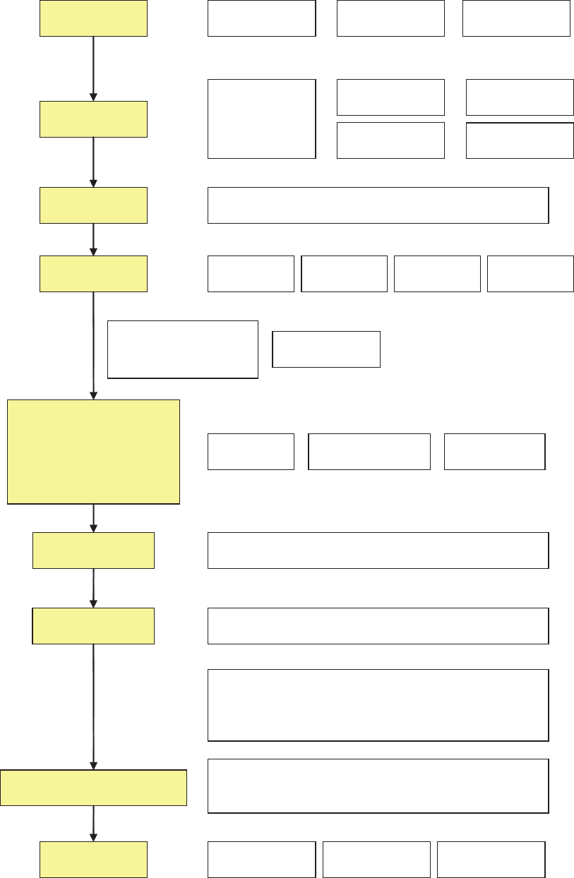
manual an overview of the steps from sampling to presenta-
tion of results to end users is presented in Fig. 1. Examples
of sampling devices are found in Figs. 2-7. In addition to
these automated sampling systems on Ships of Opportunity
(SOOP, e.g. FerryBox systems), buoys, Autonomous Under-
water Vehicles (AUV’s) etc. are used (Babin et al. 2008).
IOC Manuals & Guides no 55
Chapter 1 Introduction to methods for quantitative phytoplankton analysis
6
Quantitative
sampling
Preservation
Concentration
Storage
Printed report
Filtering Centrifugation Sedimentation
Quality control
Often made by analyst when entering data into
electronic database . Double checked by someone else
Homogenisation and DNA
extraction for some
molecular techniques
End users
Interpretation of results
Web site and
other media
Identification
of organisms
and estimation of
cell concentrations
and biomass
Microscopy Flow cytometers
Molecular biological
techniques
Lugol ’ s iodine
acid
neutral
alkaline
Aldehydes
Saline ethanol
Water bottles
( discrete depths )
Keep in dark and refrigerate . Analyse as quickly as possible
Tube
( integrating )
Sonication
Scientific
publication
Comparison with existing data, statistical analysis ,
inclusion of other data, e.g . oceanographic data
and data on algal toxins in shellfish
( None )
( None )
Results
Number of organisms or biomass per litre
and species composition ( biodiversity )
Freezing of
raw sample
Ring tests with other laboratories , test for repeatability ,
estimation of variability due to method or persons
performing analysis , documentation of methods
> accredited analysis and laboratory
Automated
sampling devices
Figure 1. Schematic drawing of the steps from sampling to results.

7
Microscopic and Molecular Methods for Quantitative Phytoplankton Analysis
Chapter 1 Introduction to methods for quantitative phytoplankton analysis
Microscopy based techniques
The historical development of microscope based
phytoplankton analysis techniques
Many historic reports exist of phytoplankton blooms. Some
believe the description of the Nile water changing to blood in
the bible and resultant fish mortalities (Exodus 7:14-25) is an
account of the occurrence of a HAB. The invention of the mi-
croscope by Anton van Leeuwenhoek (1632-1723) in the 17
th
century allowed more detailed observations of phytoplankton
to be made with Christian Gottfried Ehrenberg (1795-1876)
and Ernst Heinrich Philipp August Haeckel (1834-1919) be-
coming pioneers in observations of microalgae. Over the last
150 years a number of techniques for analysis of phytoplank-
ton have been developed and adopted in analytical laborato-
ries throughout the world. The Swedish chemist, Per Teodor
Cleve (1840-1905), was one of the first researchers to under-
take more quantitative surveys of the phytoplankton commu-
nity. He used silk plankton nets to investigate the distribution
of phytoplankton in the North Sea Skagerrak-Kattegat area
(1897). Hans Lohmann (1863-1934) first used a centrifuge
to concentrate plankton and discovered the nanoplankton
(phytoplankton 2 – 20 µm in size) (Lohmann 1911). The
classic sedimentation chamber technique still used in many
laboratories today was developed by Utermöhl (1931, 1958).
In the 1970s the fluorescence microscope was first used for
quantitative analysis of bacteria in seawater (e.g. Hobbie et al.
1977). A similar technique was used to reveal the ubiquitous
distribution of autotrophic picoplankton (size 0.2 – 2 µm) in
the sea (Johnson and Sieburth 1979, Waterbury et al. 1979).
In the 1980s auto- and heterotrophic nanoplankton were in-
vestigated using various stains and filtration techniques (e.g.
Caron 1983).
Training and literature for identification of phytoplankton
using microscopes
Microscope based methods involve the identification of phy-
toplankton species based on morphological and other visible
criteria. Phytoplankton taxonomists should have a high de-
gree of skill and experience in the identification of the spe-
cies present in their waters and appropriate training should
be incorporated into their work programme. Access to key
literature for phytoplankton identification, such as Horner
(2002), Tomas (1997) and Throndsen et al. (2003, 2007) is
essential. Access to older scientific literature is often necessary
for detailed species descriptions, however, these may be dif-
ficult to access. Attendance at phytoplankton identification
training courses when possible is the most successful way to
allow analysts to continue to learn and develop their skills.
This is especially important since the systematics and nomen-
clature of phytoplankton is constantly under revision. Species
lists and images of phytoplankton are presented in a variety
of web sites, see examples listed in Table 1. While a wealth of
information is available on the internet, they cannot replace
teaching and guidance from an experienced taxonomist.
Microscopes for phytoplankton identification and
enumeration
A high quality microscope is essential for the enumeration
and identification of phytoplankton species. Although the
initial cost will be high, a microscope, if serviced on a regular
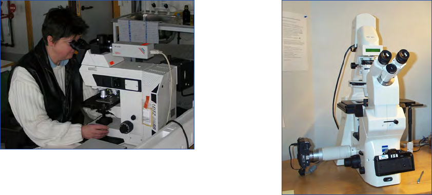
basis, can remain in use for many years. Two types of mi-
croscopes are commonly used: (1) the standard compound
(upright) microscope and (2) the inverted microscope (Figs.
8 - 9). With the inverted microscope, the objectives are posi-
tioned underneath the stage holding the sample. This is nec-
essary for examination of samples in sedimentation chambers
and flasks where the phytoplankton cells have settled onto the
bottom. Oculars should be fitted with a graticule and a stage
micrometer is used to determine and calibrate the length of
the scale bars of the eyepiece graticule under each objective
magnification. In Fig. 10 examples of how Alexandrium fun-
dyense is viewed in the microscope using different micrsocope
and staining techniques are presented. The digital photo-
graphs were taken during a workshop comparing micrsocopic
a and molecular biological techniques for quantiative phyto-
plankton analysis. Results from the workshop are found in
Godhe et al. (2007).
Because many phytoplankton species are partially transpar-
ent when viewed under a light microscope, different tech-
Species information URL
AlgaeBase www.algaebase.org
World Register of Marine Species, WoRMS www.marinespecies.org
IOC-UNESCO Taxonomic Reference List of Harmful
Micro Algae
www.marinespecies.org/hab/index.php
European Register of Marine Species, ERMS www.marbef.org
Integrated Taxonomic Information System, ITIS www.itis.gov
Micro*scope starcentral.mbl.edu/microscope/
Plankton*net www.planktonnet.eu
Encyclopedia of Life www.eol.org
Gene sequences etc.
Genbank www.ncbi.nlm.nih.gov/Genbank/
European Molecular Biological Laboratory www.embl.org
National Center for Biotechnology Information www.ncbi.nlm.nih.gov
Table 1. Examples of web sites that provide useful information for phytoplankton analysts.
IOC Manuals & Guides no 55
Chapter 1 Introduction to methods for quantitative phytoplankton analysis
8
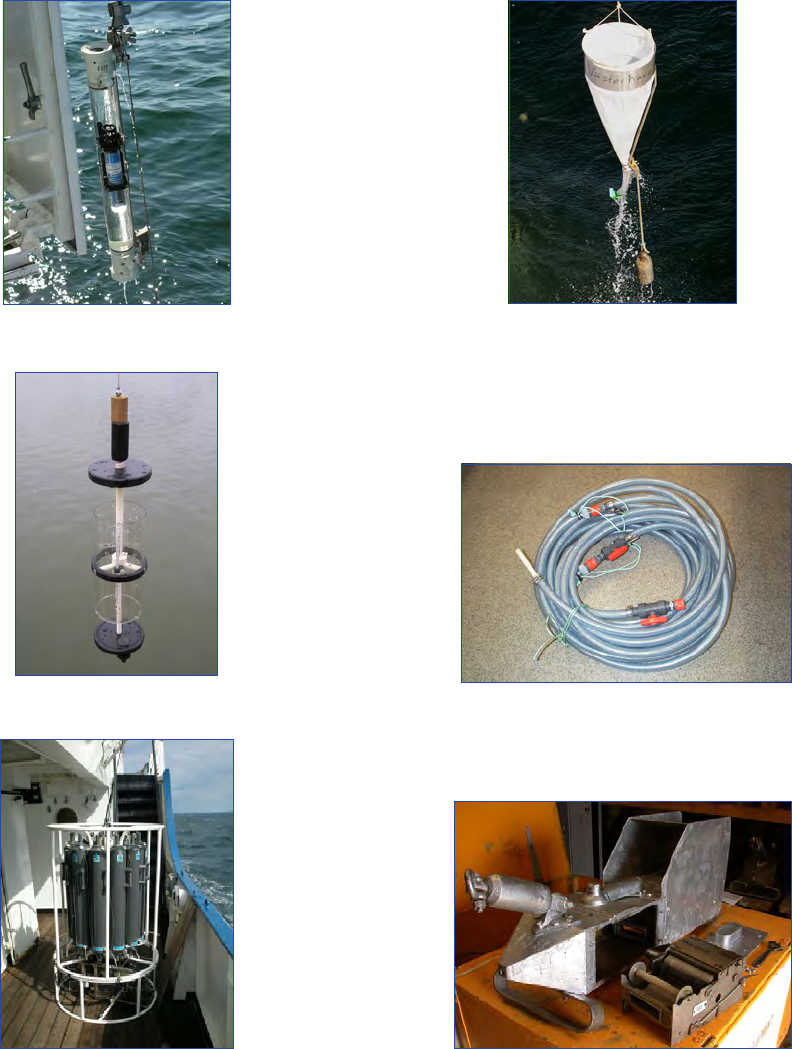
Figure 2. Reversing water sampler of the modified Nansen type.
Figure 4. CTD with rosette and Niskin-type water bottles. An in situ
chlorophyll a fluorometer is also mounted.
Figure 5. Phytoplankton net. This is not used for quantitative sampling
but for collecting rare, non fragile species.
Figure 6. Tube for integrated water sampling.
Figure 7. The Continuous Plankton Recorder. This device is mainly
aimed for sampling zooplankton but may be useful for collecting
larger, non fragile phytoplankton species. Photo courtesy of the Sir
Alister Hardy Foundation for Ocean Science, SAHFOS
http://www.sahfos.ac.uk/.
Figure 3. Water sampler of the Ruttner type.
9
Microscopic and Molecular Methods for Quantitative Phytoplankton Analysis
Chapter 1 Introduction to methods for quantitative phytoplankton analysis
niques to improve contrast are used. Differential Interference
Contrast (DIC, also called Normarski) and Phase Contrast
are popular. DIC is considered by many to be the optimal
method for general phytoplankton analysis. Most plastic con-
tainers, however, cannot be used with this method as many
plastics depolarize the required polarized light. It is also more
expensive than Phase Contrast and requires a different set of
objectives, polarizing filters etc. to function properly.
Natural fluorescence
Fluorescence generated from photosynthetic and other pig-
ments in phytoplankton can be used as an aid for the identi-
fication and enumeration of species. This works best with live
samples and samples preserved with formaldehyde or glutar-
aldehyde. If Lugols iodine is used for preservation, the natural
fluorescence is not visble. Fluorescence can also be used to dif-
ferentiate between heterotrophic and autotrophic organisms.
The microscope must be equipped with objectives suitable for
fluorescence, a lamp housing for fluorescence (e.g. mercury
lamp 50 or 100 W), the required filter sets. A useful filter set
to observe fluorescence from both chlorophyll a and phyco-
erythrin consists of a filter for excitation at 450-490 nm and a
long pass filter for emission at 515 nm.
Staining of cells
Different stains are used to aid the identification of phyto-
plankton species. In this volume only fluorescent stains (fluor-
ochromes) are discussed. The stain used in chapters 2 and 5,
calcofluor, binds to the cellulose theca in armoured dinoflag-
ellates and allows a detailed examination of the plate structure
to be performed. This stain is very useful when morphologi-
cally similar species, e.g. Alexandrium spp., are present. Fluor-
ochromes are also often used in connection with antibodies
or RNA targeted probes to identify phytoplankton. Some of
these are covered in chapter 9. It should be noted that some
microscope objective lenses do not transmit ultraviolet light
and are unsuitable for work with fluorochromes that require
UV-light excitation, e.g. calcofluor.
Image analysis
Manual phytoplankton analysis with microscopy may be time
consuming and analysts must possess the necessary skills to
allow the identification of cells using morphological features.
This has led to interest in the use of automated image analysis
of phytoplankton samples. Basic image analysis methods do
not generally discriminate between phytoplankton and other
material such as detritus and sediment in samples thereby
presenting a problem in the application to routine field sam-
ples. This technique may be more useful for the analysis of
cultures and monospecific high density blooms. Researchers
have tried more advanced methods such as artificial neural
networks (ANN) to identify species automatically by pattern
recognition. Some ANN software includes functions which
train the ANN to identify certain species. One such instru-
ment under development is the HAB Buoy, which uses the
Dinoflagellate Categorisation by Artificial Neural Network
(DICANN) recognition system software (Culverhouse et al.
2006). Other examples of software currently under evaluation
for automated phytoplankton identification are used in Flow
Cytometers (see next paragraph), e.g. the FlowCAM (chapter
8) and the method described by Sosik and Olson (2007). To
date, these methods require a highly trained phytoplankton
identification specialist to train the software to recognise the
images and carry out a quality control on the results of the
automated image analysis.
Flow cytometry
A flow cytometer is a type of particle counter initially devel-
oped for use in medical science. Today instruments have been
developed for use specifically in aquatic sciences. Autofluores-
cence and scattering properties are used to discriminate dif-
ferent types of phytoplankton. The different phytoplankton
groups are in general not well distinguished taxonomically
when a standard instrument is used. A standard flow cytom-
eter is very useful to estimate abundance of e.g. autotrophic
picoplankton. A more advanced type of flow cytometer has a
camera that produces images of each particle/organism. Auto-
mated image analysis makes it possible to identify organisms.
Manual inspection of images by an experienced phytoplank-
ton identification specialist is required for quality control and
for training the automated image analysis system. A desk top
system is described in chapter 8. An example of an in situ
system is described by Sosik and Olsen (2007) and Olsen and
Sosik (2007).
Molecular techniques
Significance of molecular based phytoplankton analysis
techniques
Owing to some of the difficulties and limitations of mor-
phological identification techniques, microalgal studies are
increasingly exploring the use of molecular methods. Most
molecular techniques have their origin in the medical science,
and during the last three decades these various techniques
have been tested, modified, and refined for the use in algal
identification, detection and quantification.
The development of molecular tools for the identification and
detection of microalgae has influenced and improved other
fields of phycological research. Molecular data are gaining in-
fluence when the systematic position of an organism is estab-
lished. Today, the description of new species, erection of new
genera, or rearrangement of a species to a different genus is
usually supported by molecular data in addition to morpho-
logical structures, ultrastructure, and information on biogeo-
graphic distribution (e.g. Fraga et al. 2008). Thus, the un-
derstanding of evolutionary relationships among microalgal
taxa has been immensely improved (Saldarriaga et al. 2001).
Spatially separated populations of microalgal species might
display different properties, such as toxin production. By
studying minor differences within the genome, populations
can be confined to certain locations, and human assisted and/
or natural migration of populations can be investigated (e.g.
Persich et al. 2006, Nagai et al. 2007). Also, the increasing
information on the structure of genes and new tools for inves-
tigating their expressions, have enhanced our understanding
of algal physiological processes (Maheswari et al. 2009).
Laboratory requirements for molecular techniques
Different types of molecular techniques have very different
requirements for laboratory facilities and instruments. The
range is from very well equipped laboratories to field instru-
ments. In chapters 9-14 examples of laboratory methods are
IOC Manuals & Guides no 55
Chapter 1 Introduction to methods for quantitative phytoplankton analysis
10
found. In situ systems are under development (e.g. Paul et al.
2007 and Scholin et al. 2009).
Identification and quantification of phytoplankton species
by molecular methods
Molecular methodologies aim to move away from species
identification and classification using morphological charac-
teristics that often require highly specialist equipment such as
electron microscopes, or very skilled techniques such as single
cell dissections. Instead molecular techniques exploit differ-
ences between species at a genetic level. Molecular analysis
requires the use of specialised equipment and personnel and
most importantly requires a previous knowledge of the genet-
ic diversity of the phytoplankton in a specific region. To date,
molecular methods have been used to support HAB monitor-
ing programmes in New Zealand and the USA (Rhodes et al.
1998, Scholin et al. 2000, Bowers et al. 2006).
In this present manual, methods based on ribosomal RNA
(rRNA) and DNA (rDNA) targeted oligonucleotides and
polymerase chain reaction (PCR) are described. Oligonucle-
otides and PCR primers are short strains of synthetic RNA or
DNA that is complementary to the target RNA/DNA. Mo-
lecular sequencing of phytoplankton cells has generated DNA
sequence information from many species around the world.
This has allowed the design of oligonucleotide probes and
PCR primers for specific microalgal species. Some oligonu-
cleotide probes, which hybridize with complementary target
rRNA or rDNA, have a fluorescent tag attached and can act
as a direct detection method using fluorescence microscopy.
PCR primers enable the amplification of target genes through
PCR. The primers serve as start and end points for in vitro
DNA synthesis, which is catalysed by a DNA polymerase.
The PCR consists of repetitive cycles, where in the first step,
DNA is heated in order to separate the two strands in the
DNA helix. In the second step during cooling, the primers,
which are present in large excess, are allowed to hybridize with
the complementary DNA. In a third step, the DNA polymer-
ase and the four deoxyribonucleoside triphosphates (dNTPs)
complete extension of a complementary DNA strand down-
stream from the primer site. For effective DNA amplifica-
tion, the three steps are repeated in 20-35 cycles (Alberts et
al. 1989). A useful volume covering the basics of molecular
methods and general applications is Molecular Systematics
edited by Hillis et al. (1996).
Most of the molecular methods described here, with the ex-
ception of the whole cell assay (chapter 9 and 14), do not
require the cells to remain intact. In these methods the rRNA
molecules in the cell’s cytoplasm or the nuclear DNA are re-
leased during nucleic acid extraction and are targeted by the
probes or PCR primers. During the whole cell assay, the target
rRNA/rDNA within intact cells is labelled with fluorescently
tagged probes. It is therefore vital that the laboratory protocol
used ensures that the probes can penetrate the cell wall in
order to access target genetic region and label them. Tyramide
Signal Amplification has been used with FISH (TSA-FISH)
to further enhance fluorescence signals (see chapter 14). The
fluorescent tag can then be read using a fluorescent micro-
scope as with the whole cell assays (FISH chapter 9) or addi-
tional technology is employed to allow these fluorescent tags
to be read automatically e.g. using a sandwich hybridization
technique (chapter 12) and PCR (chapter 13).
The hand held device and DNA-biosensor with disposable
sensorchip (sandwich hybridisation, electrochemical detec-
tion) and DNA microarray technology (fluorescent detec-
tion) methods discussed in this manual are still at the final
development stages (see chapters 10 and 11). Within the
next decade these methods may be ready to be incorporated
into monitoring programmes. The authors suggest that fu-
ture advances in this field will include microarray/DNA chip
(sometimes called “phylochips”) technologies with probes for
multiple species applied in situ to an environmental sample
simultaneously.
Alternative molecular based methods such as lectin (protein
and sugar) binding and antibody based assays (e.g. immuno-
fluorescence assays) are not included in this manual. Infor-
mation on these molecular diagnostic tools may be found
in chapter 5 of The Manual on Harmful Marine Microalgae
(Hallegraeff et al. 2004).
Molecular method validation
rDNA and rRNA have become the most popular target re-
gions for microalgal species identification. These regions are
attractive for primer and probe design because they contain
both conserved and variable regions and are ubiquitous in
Figure 8 Compound microscope
Figure 9. Inverted microscope
11
Microscopic and Molecular Methods for Quantitative Phytoplankton Analysis
Chapter 1 Introduction to methods for quantitative phytoplankton analysis
all organisms. In addition, a large number of sequences are
available in molecular web based databases, e.g. GENBANK,
for sequence comparative analyses (Table 1) and design of
oligonucleotide probes and PCR primers. Despite extensive
sequence analysis of cultured phytoplankton species, cross
reactivity with other organisms in the wild may occur, it is
therefore crucial to test the developed probes/primers with
the target species and several non-target species. Method
development, although time consuming, is essential if these
methods are to be implemented. It is the responsibility of the
end user to ensure that specificity to the target organism is
evaluated appropriately.
Quality control
As with all scientific research, it is necessary to investigate the
variability of the methods used before employment into any
monitoring programme. The variability of the result can be
affected by cell abundance which can dictate the method of
choice. Further information on this can be found in chapter
2 and of Venrick (1978 a,b,c) and Andersen and Throndsen
(2004). Many laboratories have achieved national accredita-
tion for techniques described in this manual. This involves
developing protocols with levels of traceability and reproduc-
ibility in line with defined criteria. Participation in interna-
tionally recognised inter-laboratory comparisons are strongly
recommended.
References
Alberts B, Bray D, Lewis J, Raff M, Roberts K, Watson JD (1989)
Molecular biology of the cell. Garland Publishing, Inc, New York,
1219 p.
Andersen P, Throndsen J (2004) Estimating cell numbers. In: Halle-
graeff GM, Anderson DM, Cembella AD (eds) Manual on Harm-
ful Marine Microalgae. UNESCO, Paris, pp. 99-129.
Babin M, Roesler C, Cullen JJ (eds) (2008) Real-time coastal ob-
serving systems for marine ecosystem dynamics and harmful al-
gal blooms: theory, instrumentation and modelling, UNESCO
monographs on oceanographic methodology UNESCO Publish-
ing, 860 p.
Bowers HA, Trice MT, Magnien RE, Goshorn DM, Michael B,
Schaefer EF, Rublee PA, Oldach DW (2006) Detection of Pfies-
teria spp. by PCR in surface sediments collected from Chesapeake
Bay tributaries (Maryland) Harmful Algae 5(4): 342-351
Caron DA (1983) Technique for enumeration of heterotrophic and
phototrophic nanoplankton, using epifluorescence microscopy,
and comparison with other procedures. Appl. Environ. Microbiol.
46, 491-498.
Culverhouse PF, Williams R, Simpson B, Gallienne C, Reguera B,
Cabrini M, Fonda-Umani S, Parisini T, Pellegrino FA, Pazos Y,
Wang H, Escalera L, Moroño A, Hensey M, Silke J, Pellegrini A,
Thomas D, James D, Longa MA, Kennedy S, del Punta G (2006)
HAB Buoy: a new instrument for in situ monitoring and early
warning of harmful algal bloom events African Journal of Marine
Science 28(2): 245–250
Field CB, Behrenfeld MJ, Randerson JT, Falkowski PG (1998) Pri-
mary production of the biosphere: Integrating terrestrial and oce-
anic components. Science 281, 237–240.
Fraga S, Penna A, Bianconi I, Paz B, Zapata M (2008) Coolia cana-
riensis sp nov (Dinophyceae), a new nontoxic epiphytic benthic
dinoflagellate from the Canary Islands. Journal of Phycology 44:
1060-1070
Franks PJS, Keafer BA (2004) Sampling techniques and strategies
for coastal phytoplankton blooms. In: Hallegraeff, G.M., Ander-
son, D.M., Cembella, A.D. (eds), Manual on Harmful Marine
Microalgae. UNESCO, Paris, pp. 51 - 76.
Godhe A, Cusack C, Pedersen J, Andersen P, Anderson DM, Bresnan
E, Cembella A, Dahl E, Diercks S, Elbrächter M, Edler L, Gal-
luzzi L, Gescher C, Gladstone M, Karlson B, Kulis D, LeGresley
M, Lindahl O, Marin R, McDermott G, Medlin LK, Naustvoll
L-K, Penna A, Töbe K (2007) Intercalibration of classical and mo-
lecular techniques for identification of Alexandrium fundyense (Di-
nophyceae) and estimation of cell densities. Harmful Algae: 56-72
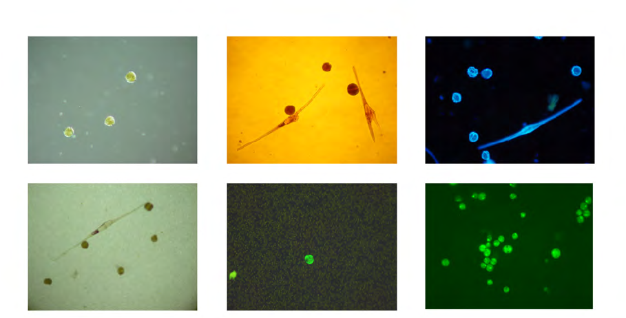
Figure 10. Alexandrium fundyense as seen in the microscope using different techniques. Ceratium spp. are present in B, C and D. A. Filter
freeze transfer with contrast enhancement using DIC (appearance in Utermöhl is essentially identical), B. Sedimentation flask, C. Filtering
+ calcofluor staining, D. Filtering using semitransparent filters, E.and F. Whole cell hybridization assay.
Sample preparation: A. Allan Cembella, B. Georgina McDermott, C. Per Andersen, D. Einar Dahl, E. Melissa Gladstone and F. David Kulis.
F is originally a greyscale image to which artificial colour has been added to simulate what the eye sees. Photo A-E Bengt Karlson and F
David Kulis. Microscope. A-E Zeiss Axiovert 200 and F Zeiss Axioplan 40 Fl.
A CB
D E F
IOC Manuals & Guides no 55
Chapter 1 Introduction to methods for quantitative phytoplankton analysis
12
Hallegraeff GM, Anderson DM, Cembella AD (1995) Manual on
Harmful Marine Microalgae. UNESCO, Paris, 551 pp.
Hallegraeff GM, Anderson DM, Cembella AD (2004) Manual on
Harmful Marine Microalgae. UNESCO, Paris, 793 pp.
Hillis D, Moritz C, Mable B (eds) (1996) Molecular systematics,,
Sinauer Associates, Sunderland, 655 pp.
Hobbie JE, Daley RJ, Jasper S (1977) Use of Nuclepore filters for
counting bacteria by fluorescence microscopy. Appl. Environ.
Microbiol. 33: 1225-1228.
Horner RA (2002) A Taxonomic Guide to Some Common Marine
Phytoplankton, Bristol, UK, 195 pp.
Johnson PW, Sieburth JM (1979) Chroococcoid cyanobacteria in
the sea: A ubiquitous and diverse phototrophic biomass. Limnol.
Oceanogr. 24: 928-935.
Lohmann H (1911) Über das nannoplankton und die Zentrifugie-
rung kleinster Wasserproben zur Gewinnung desselben in leben-
dem Zustande. Int. Revue ges. Hydrobiol. 4: 1-38.
Maheswari U, Mock T, Armbrust EV, Bowler C (2009) Update of
the Diatom EST Database: a new tool for digital transcriptomics.
Nucleic Acids Research 37: D1001-D1005.
Nagai S, Lian C, Yamaguchi S, Hamaguchi M, Matsuyama Y, Ita-
kura S, Shimada H, Kaga S, Yamauchi H, Sonda Y, Nishikawa
T, Kim C-H, Hogetsu T (2007) Microsatellite markers reveal
population genetic structure of the toxic dinoflagellate Alexandri-
um tamarense (Dinophyceae) in Japanese coastal water. Journal of
Phycology 43: 43-54
Olson RJ, Sosik HM (2007) A submersible imaging-in-flow instru-
ment to analyze nano- and microplankton: Imaging FlowCyto-
bot. Limnol. Oceanogr. Methods, 5: 195-208.
Paul J, Scholin C, van den Engh G, Perry MJ (2007) A sea of mi-
crobes. In situ instrumentation. Oceanogr. 2(2): 70-78.
Persich G, Kulis D, Lilly E, Anderson D, Garcia V (2006) Probable
origin and toxin profile of Alexandrium tamarense (Lebour) Balech
from southern Brazil. Hamful Algae 5: 36-44
Platt T, Li WKW (1986) Photosynthetic picoplankton. Minister of
Supply and Services, Canada, Ottawa, 583 pp.
Rhodes L, Scholin C, Garthwaite I (1998) Pseudo-nitzschia in New
Zealand and the role of DNA probes and immunoassays in re-
fining marine biotoxin monitoring programmes. Natural Toxins
6:105-111.
Saldarriaga JF, Taylor FJR, Keeling PJ, Cavalier-Smith T (2001)
Dinoflagellate nuclear SSU rRNA phylogeny suggests multiple
plastid losses and replacements. Journal of Molecular Evolution
53
Scholin CA, Gulland F, Doucette GJ, Benson S, Busman M, Chavez
FP, Cordaro J, DeLong R, De Vogelaere A, Harvey J, Haulena M,
Lefebvre K, Lipscomb T, Loscutoff S, Lowenstine LJ, Martin R
I, Miller PE, McLellan WA, Moeller PDR, Powell CL, Rowles T,
Silvagnl P, Silver M, Spraker T, Van Dolah FM (2000) Mortality
of sea lions along the central coast linked to a toxic diatom bloom.
Nature 403: 80-84.
Scholin C, Doucette G, Jensen S, Roman B, Pargett D, Marin II R,
Preston C, Jones W, Feldman J, Everlove C, Harris A, Alvarado
N, Massion E, Birch J, Greenfield D, Vrijenhoek R, Mikulski C,
Jones K (2009) Remote detection of marine microbes, small in-
vertebrates, harmful algae, and biotoxins using the Environmental
Sample Processor (ESP). Oceanography 22: 158-167.
Simon N, Barlow RG, Marie D, Partensky F, Vaulot D (1994) Char-
acterization of oceanic photosynthetic picoeukaryotes by flow cy-
tometry, J. Phycol. 30: 922-935.
Simon N, Cras A-L, Foulon E, Lemée R (2009) Diversity and evolu-
tion of marine phytoplankton, C. R. Biologies 332: 159-170
Sosik HM, Olson RJ (2007) Automated taxonomic classification of
phytoplankton sampled with image-in-flow cytometry. Limnol.
Oceanogr. Methods. 5: 204-216.
Sournia A (ed.) 1978. Phytoplankton manual. UNESCO, Paris,
337pp.
Tomas CR (ed.) 1997, Identifying Marine Phytoplankton, Academ-
ic, Press, San Diego, 858 pp.
Throndsen J, Hasle GR, Tangen K (2003) Norsk kystplanktonflora.
Almater forlag AS, Oslo, 341 pp. (in Norwegian).
Throndsen J, Hasle GR, Tangen K (2007) Phytoplankton of Norwe-
gian coastal waters, Almater forlag AS, Oslo, 343 pp.
Utermöhl H (1931) Neue Wege in der quantitativen Erfassung des
Planktons (mit besonderer Berücksichtigung des Ultraplanktons).
Verh. int. Ver. theor. angew. Limnol. 5: 567-596.
Utermöhl H (1958) Zur Vervollkomnung der quantitativen Phyto-
plankton-Methodik. Mitt. int. Ver. ther. angew. Limnol. 9: 1-38.
Waterbury JB, Watson SW, Guillard RRL, Brand LE (1979) Wide-Wide-
spread occurrence of a unicellular, marine, planktonic, cyanobac-
terium. Nature 227: 293-294.
Venrick EL (1978a) How many cells to count? In: Sournia, A. (ed),
Phytoplankton manual. UNESCO, Paris, pp. 167-180.
Venrick EL (1978b) The implications of subsampling. In: Sournia A
(ed) Phytoplankton manual. Unesco, Paris, pp. 75-87.
Venrick E, (1978c) Sampling design. In: Sournia, A. (Ed.),
Phytoplankton manual. Unesco, Paris, pp. 7-16.

13
Microscopic and Molecular Methods for Quantitative Phytoplankton Analysis
Chapter 2 The Utermöhl method
2 The Utermöhl method for quantitative phytoplankton analysis
Lars Edler*
1
and Malte Elbrächter
2
1
WEAQ, Doktorsgatan 9 D., SE-262 52 Ängelholm, Sweden
2
Deutsches Zentrum für Marine Diversitätsfor-schung Forschungsinstitut Senckenberg, Wattenmeerstation Sylt, Hafenstr. 43, D-25992
List/Sylt, Germany
*Author for correspondence: e-mail [email protected]
Introduction
The Utermöhl method (Utermöhl 1931, 1958) has an ad-
vantage over other methods of phytoplankton analysis in that
algal cells can be both identified and enumerated. Using this
method, it is also possible to determine individual cell size,
form, biovolume and resting stage.
The Utermöhl method is based on the assumption that cells
are poisson distributed in the counting chamber. The method
is based on the sedimentation of an aliquot of a water sample
in a chamber. Gravity causes the phytoplankton cells to settle
on the bottom of the chamber. The settled phytoplankton
cells can then be identified and enumerated using an inverted
microscope. To quantify the result as cells per Litre a conver-
sion factor must be determined.
Materials
Equipment
Sample Bottles
If samples are analysed immediately or within a few days
plastic vials may be used. Note that the preservatives may be
absorbed by the plastic. For long term storage, glass sample
bottles should be used to minimise any chemical reaction
with the preservative. Clear glass bottles allow the state of
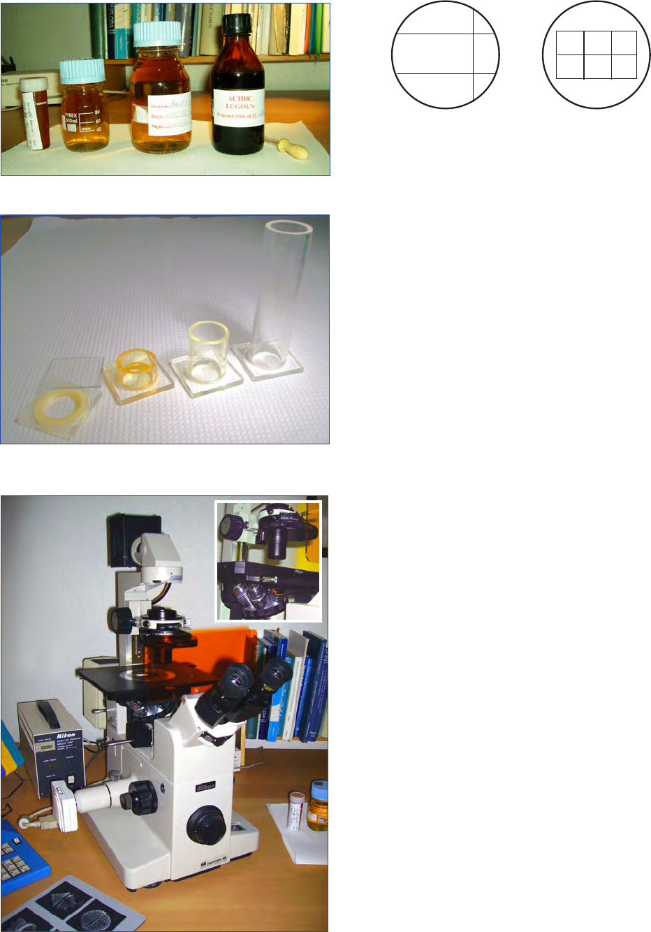
Lugol’s iodine preservation to be easily monitored (Fig. 1).
These samples must be stored in the dark to prevent the de-
gradation of Lugol’s iodine in light. It is important that the
bottle cap is securely tightened to avoid spillage of the sample
and evaporation of the preservative. Utermöhl (1958) recom-
mended that the bottle is filled to 75-80% of its volume. This
facilitates the homogenisation of the sample before dispensing
into the sedimentation chamber.
Preservation agents
Preservation agents must be chosen depending on the objec-
tive of the study. The most commonly used is potassium iodi-
ne; Lugol’s iodine solution – acidic, neutral or alkaline (Table
1; Andersen and Throndsen 2004). If samples are stored for
long periods they may be preserved with neutral formalde-
hyde (Table 2).
Sedimentation chambers
The sedimentation chamber consists of two parts, an upper
cylinder (chimney) and a bottom plate with a thin glass (Fig.
2). They are usually made of perspex in volumes of 2, 5, 10,
25 or 50 mL. The thickness of the glass base plate should not
exceed 0.2 mm, as this will affect the resolution achievable
by the microscope. Counting chambers should be calibrated.
This is achieved by first weighing the chamber while empty
and then filled with water to confirm the volume.
The inverted microscope
For quantitative analysis using sedimentation chambers, an
inverted microscope is required (Fig. 3). The optical quality of
the microscope is crucial for facilitating phytoplankton iden-
tification. Phase- and/or differential interference-contrast is
helpful for the identification of most phytoplankton, whereas
bright-eld may be advantageous for coccolithophorids (He-
imdahl 1978).
Epifluorescence equipment is a great advantage for counting
and identification of organisms with cellulose cell walls, e.g.,
thecate dinoflagellates, chlorophytes and “fungi”. A stain is
applied to the sample which causes cellulose to fluoresce.
One eyepiece should be equipped with a calibrated ocular
micrometer. The other eyepiece should be equipped with
two parallel threads forming a transect. A third thread per-
pendicular to the other two facilitates the counting procedure
(Fig. 4 a). It is also possible to have the eyepiece equipped
with other graticules such as a square field or grids (Fig. 4
b). The eyepiece micrometer and counting graticule must be
calibrated for each magnification using a stage micrometer.
Acidic Alkaline Neutral
20 g potassium iodide (KI) 20 g potassium iodide (KI) 20 g potassium iodide (KI)
10 g iodine (I
2
) 10 g iodine (I
2
) 10 g iodine (I
2
)
20 g conc. acetic acid 50 g sodium acetate 200 mL distilled water
200 mL distilled water 200 mL distilled water
Table 1. Recipes for Lugol’s iodine solution (acidic, alkaline and neutral).
(from: Utermöhl 1958, Willén 1962, Andersen and Throndsen, 2004).
Table 2. Recipe for neutral formaldehyde. (from: Throndsen 1978,
Edler 1979, Andersen and Throndsen 2004). Filter after one week
to remove any precipitates.
Neutral formaldehyde
500 mL 40% formaldehyde
500 mL distilled water
100 g hexamethylentetramid
pH 7.3 – 7.9

IOC Manuals & Guides no 55
Chapter 2 The Utermöhl method
14
Scope
Qualitative and quantitative analysis of phytoplankton.
Detection range
Detection range is dependent on the volume of sample settled.
Counting all of the cells in a 50 mL chamber will give a detec-
tion limit of 20 cells per Litre.
Advantages
Qualitative as well as quantitative analysis. Identification and
quantification of muliple or single species. Detection of harm-
ful species.
Drawbacks
This is a time consuming analysis that requires skilled person-
nel. Sedimentation time prevents the immediate analysis of
samples. Autotrophic picoplankton is not analysed using the
Utermöhl method.
Type of training needed
Analysis requires continuous training over years with in-depth
knowledge of taxonomic literature.
Essential Equipment
Inverted microscope, sedimentation chambers, microscope
camera, identification literature, (epifluorescense equipment,
counting programme).
Equipment cost*
Inverted microscope: 7,500 – 50,000 € (11,000 – 70,000 US $).
Sedimentation chamber: 150 € (200 US$).
Microscope camera: 3,000 – 8,000 € (4,300 – 11,000 US $).
Identification literature: 1,000 – 3,000 € (1,400 – 4,300 US $).
Epifluorescense equipment: 10,000 € (14,000 US $).
Counting programme: 500 – 5,000 € (700 – 7,000 US $).
Consumables, cost per sample**
Less than 5 €/4 US $.
Processing time per sample before analysis
App. 10 minutres for filling and assembling sedimentation
chamber.
3-24 hours sedimtation time depending on volume and analysis
type.
Analysis time per sample
2-10 hours or more depending on type of sample and analysis.
Sample throughput per person per day
1-4 depending on type of sample and analysis.
No. of samples processed in parallel
One per analyst.
Health and Safety issues
Analysis sitting at the microscope is tiresome for eyes, neck and
shoulder. Frequent breaks are needed. If formalin is used as pre-
servation agent appropriate health and safety guidelines must
be followed.
*service contracts not included
**salaries not included
The fundamentals of
The Utermöhl method
15
Microscopic and Molecular Methods for Quantitative Phytoplankton Analysis
Chapter 2 The Utermöhl method
The microscope should have objectives of 4-6X, 10X, 20X
and 40-60X. For detailed examination a 100X oil immersion
objective may also be used. If epifluorescence microscopy is
to be used, the microscope must be equipped with the appro-
priate objective lenses. In order to survey the entire bottom
plate the microscope must be equipped with a movable me-
chanical stage.
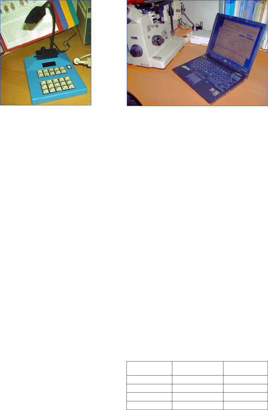
Cell counters
A cell counter with 12 or more keys is a useful device. Medical
blood cell counters (Fig. 5) are commonly used. If these are
not availabe single tally counters can be used as appropriate. It
is also common to have a computerised counting programme
(Fig. 6) beside the microscope, so that the observed species are
registered directly into a database.
Laboratory facilities
Laboratory facilities necessary for the quantitative analysis
of phytoplankton require amenities for storing, handling
(mixing and pouring samples) and washing of sedimentation
chambers. Preserved samples should be stored in cool and
dark conditions. During sedimentation the chambers should
be placed on a level, horizontal and solid surface. This will
prevent any non random accumulation of phytoplankton cells.
Methods
Preparation of sample
Preservation
Once the sample has been collected from the field and poured
into the sample bottle it should be immediately preserved
using either:
Lugol’s iodine solution;
0.2 – 0.5 mL per 100 mL water sample.
Neutralised formaldehyde;
2 mL per 100 mL water sample.
The advantage of Lugol’s iodine solution is that it has an in-
stant effect and increases the weight of the organisms redu-
cing sedimentation time. Lugol’s iodine solution will cause
discolouration of some phytoplankton making identification
difficult. To reduce this effect, the sample can be bleached us-To reduce this effect, the sample can be bleached us-
ing sodium thiosulfate prior to analysis.
The advantage of formaldehyde is that preserved samples re-
main viable for a long time. Formaldehyde is not suitable for
fixation of naked algal cells, as the cell shape is distorted and
flagella are lost. Some naked algal forms may also disintegra-
te when formaldehyde is used (CEN 2005). Formaldehyde
should be used with care because of its toxicity to humans
(Andersen and Throndsen 2004).
Figure 1. Sample bottles: glass and plastic. Bottle of Lugol’s iodine
solution to the right.
Figure 2. Sedimentation chambers. From left to right: bottom plate
with cover glass, 10 mL chamber, 25 mL chamber and 50 mL
chamber.
Figure 3. Inverted microscope.
Figure 4. Counting aids mounted in the eyepiece. a) parallel
threads, with a transverse thread. b) grids.
A B
IOC Manuals & Guides no 55
Chapter 2 The Utermöhl method
16
Storage of samples
Preserved phytoplankton samples should be stored in cool
and dark conditions. When using Lugol’s iodine solution, the
colour of the sample should be checked regularly and if neces-
sary, more preservative added. Preserved samples should be
analysed without delay. Samples stored more than a year are
of little use (Helcom Combine 2006).
Temperature adaptation
The first step in the analysis procedure is to adapt the
phytoplankton sample and the sedimentation chamber to
room temperature. This prevents convection currents and air
bubbles forming in the sedimentation chamber. If this is not
carried out non-random settling of the phytoplankton cells
may occur.
Chamber preparation
Sediment chambers must be clean and dust free to avoid con-
tamination from previous samples. Many laboratories use a
new base plate after every sample. Sometimes it is necessary
to grease the chimney bottom with a small amount of vaseline
to ensure the chamber parts are tightly sealed (Andersen and
Throndsen 2004).
In studies where the succession of the phytoplankton is exa-
mined over a period of time it is important to use the same
chamber volume for the analysis (Hasle 1978a). At times, the
“standard” chamber size may be either too small (extreme
winter situations) or too large (phytoplankton blooms) and
another chamber size must be used.
Sample homogenisation
Before the sample is poured into the sedimentation chamber,
the bottle should be shaken firmly, but gently, in irregular
jerks to homogenise the contents. Violent shaking will pro-
duce bubbles, which can be difficult to eliminate. A rule of
thumb is to shake the bottle at least 50 times. It is recom-It is recom-
mended to check the homogenous distribution a couple of
times per year by counting 3 subsamples from the same stock-
sample.
Concentration/dilution of samples
Although it is possible to concentrate and dilute samples that
are either too sparse or too dense it is not recommended as
all additional handling steps may interfere with the sample
contents. Instead it is recommended that a sediment chamber
of an appropriate size be used to allow accurate identification
and enumeration of cells.
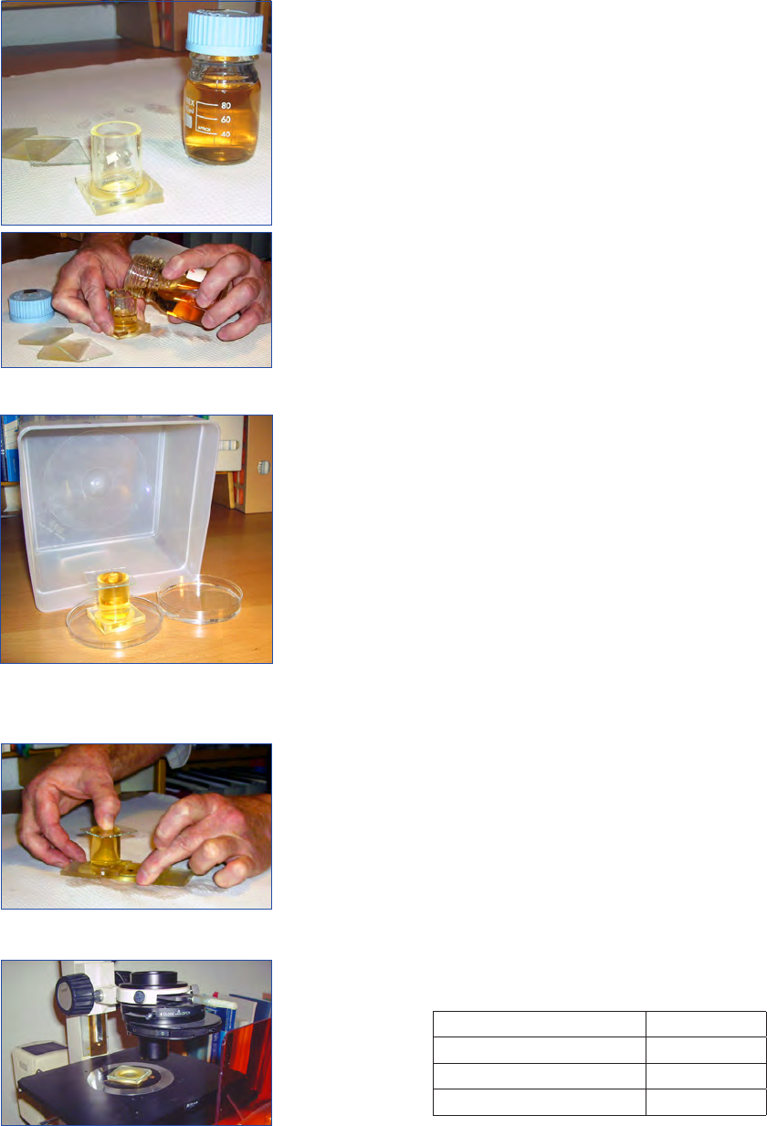
Filling the sedimentation chamber
After homogenisation, the sedimentation chamber is placed
on a horizontal surface and gently filled from the sample
bottle (Fig. 7a and 7b). The chamber is then sealed with a
cover glass. It is important that no air bubbles are left in the
chamber. It may be necessary to grease the cover glass with a
little vaseline to maintain a tight seal.
Sedimentation
The sedimentation should take place at room temperature
and out of direct sunlight. In order to minimise evaporation
the sedimentation chamber may be covered with a plastic box
and a Petri dish containing water should be placed beside the
chamber (Fig. 8). Settling time is dependent on the height
of the chamber and the preservative used (Lund et al. 1958,
Nauwerck 1963). Recommended settling times for Lugol’s
preserved samples are shown in Table 3. According to Hasle
(1978a) formaldehyde preserved samples need a settling time
of up to 40 hours independent of chamber size.
After sedimentation the chimney of the sedimentation cham-
ber is gently slid off from the bottom plate and replaced by a
cover glass. Care should be taken not to introduce airbubbles
at this stage (Fig. 9). The transfer of the bottom plate to the
microscope will not affect the distribution of the settled phy-
toplankton cells if there are no air bubbles present. The bot-
tom plate is placed on the inverted microscope (Fig. 10) and
the phytoplankton cells are identified and counted.
Figure 5. Laboratory cell counter.
Figure 6. Computerised counting programme.
Table 3. Recommended settling times for Lugol’s iodine preserved
samples (from Edler 1979).
Chamber volume
(mL)
Chamber height
approx. (cm)
Settling time (hr)
2 1 3
10 2 8
25 5 16
50 10 24
17
Microscopic and Molecular Methods for Quantitative Phytoplankton Analysis
Chapter 2 The Utermöhl method
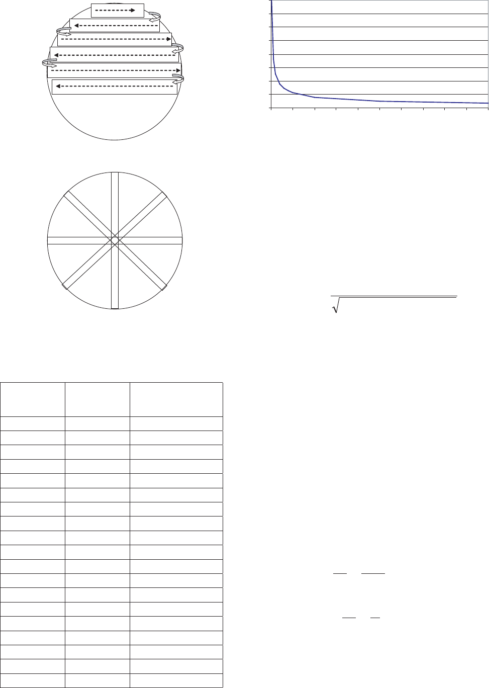
Counting procedure
The quantitative analysis should start with a scan of the entire
chamber bottom at a low magnification. This will help to give
an overview of the density and distribution of phytoplankton.
If the distribution is considered uneven the sample must be
discarded. During this scan it is also convenient to make a
preliminary species list, which may help to select the counting
strategy.
Organisms should be identified to the lowest taxonomic le-
vel that time and skill permits (Hasle 1978b). Ultimately the
objective of the study will decide the level of identification
accuracy.
Counting begins at the lowest magnification, followed by ana-
lysis at successively higher magnification. For adequate com-
parison between samples, regions and seasons it is important
to always count the specific species at the same magnification.
In special situations, such as bloom conditions, however, this
may not be possible. Large species which are easy to identify
(e.g. Ceratium spp.) and also usually relatively sparse can be
counted at the lowest magnification over the entire chamber
bottom. Smaller species are counted at higher magnifications,
and if needed, only on a part of the chamber bottom. In Table
4, the recommended magnifications for different phytoplank-
ton sizes are listed.
Counting the whole chamber bottom is done by traversing
back and forth across the chamber bottom. The parallel ey-
epiece threads delimit the transect where the phytoplankton
are counted (Fig. 11).
Counting part of the chamber bottom can be done in diffe-
rent ways. If half the chamber bottom is to be analysed every
second transect of the whole chamber is counted. If a smaller
part is to be analysed one, two, three or more diameter tran-
sects are counted. After each transect is counted the chamber
is rotated 25-45
o
(Fig. 12).
When counting sections of the chamber using transects it
is important to be consistent as to which cells lying on the
border lines are to be counted. The easiest way is to decide
that cells lying on the upper or right line should be counted,
whereas cells on the lower or left line should be omitted.
In order to obtain a statistically robust result from the quanti-
tative analysis it is necessary to count a certain number of
counting units (cells, colonies or filaments). The precision
Table 4. Recommended magnification for counting of different size
classes of phytoplankton (Edler, 1979, Andersen and Throndsen
2004).
Size class Magnification
0.2 – 2.0 µm (picoplankton)* 1000 x
2.0 – 20.0 µm (nanoplankton) 100 – 400 x
>20.0 µm (microplankton) 100 x
* picoplankton are normally not analysed using
the Utermöhl method.
Figure 8. Sedimentation, with a Petri dish filled with water. A
plastic box covers the sedimentation chamber and the Petri dish to
maintain the humidity.
Figure 9. Replacing the sedimentation chimney with a cover glass.
Figure 10. Chamber bottom placed in microscope ready for
analysis.
Figure 7A and 7B. Filling of sedimentation chamber.
A
B
IOC Manuals & Guides no 55
Chapter 2 The Utermöhl method
18
desired decides how many units to count. The precision is
usually expressed as the 95% confidence limit as a propor-
tion of the mean. Table 5 and Figure 13 show the relationship
between number of units counted and the accuracy. In many
studies it has been decided that counting of 50 units of the
dominant species, giving a 95% confidence limit of 28% is
sufficient. Increasing the precision to e.g. 20% or 10% would
need a dramatic increase in counted units, 100 and 400 re-
spectively (Venrick 1978, Edler 1979). The precision is given
by the following equation:
It is clear that it will not be possible to count 50 units of all
species present in a sample. Some species may not be suffi-
cently abundant which will decrease the overall precision. To
maintain an acceptable precision for the entire sample a total
of at least 500 units should be counted (Edler 1979).
The counting unit of most phytoplankton species is the cell.
In some cases this is not practical. For filamentous cyano-
bacteria, for instance, the practical counting unit is a certain
length of the filament, usually 100 µm (Helcom Combine
2006). In some colony forming species and coenobia it may
be difficult to count the individual cells. In such cases the co-
lony/coenobium should be the counting unit. If desired, the
calculation of cells per colony/coenobium can be approxima-
ted by a thorough counting and mean calculation of a certain
number of colonies/coenobia.
The transformation of the microscopic counts to the concen-
tration or density of phytoplankton of a desired water volume
(usually Litre or millilitre) can be achieved using this equa-
tion:
V: volume of counting chamber (mL)
A
t
: total area of the counting chamber (mm
2
)
A
c
: counted area of the counting chamber (mm
2
)
N: number of units (cells) of specific species counted
C: concentration (density) of the specific species
Table 5. Relationship between number of cells counted and
confidence limit at 95% significance level (Edler 1979, Andersen
and Throndsen 2004).
No of counted
cells
Confidence limit
+/- (%)
Absolute limit if cell
density is estimated at
500 cells L
-1
1 200 500 ± 1000
2 141 500 ± 705
3 116 500 ± 580
4 100 500 ± 500
5 89 500 ± 445
6 82 500 ± 410
7 76 500 ± 380
8 71 500 ± 355
9 67 500 ± 335
10 63 500 ± 315
15 52 500 ± 260
20 45 500 ± 225
25 40 500 ± 200
50 28 500 ± 140
100 20 500 ± 100
200 14 500 ± 70
400 10 500 ± 50
500 9 500 ± 45
1000 6 500 ± 30
Figure 12. Counting of diameter transects.
Figure 11. Counting of the whole chamber bottom with the parallel
eyepiece threads indicating the counted area.
Figure 13. Relationship between number of cells counted and
confidence limit at the 95% significance level.
0
25
50
75
100
125
150
175
200
0 50 100 150 200 250 300 350 400 450 500
no of counted cells
Confidence limit (%)
countedcellsofnumber
100*2
%Precision =
V A
A
N mLCells
c
t
1
* *
1
−
V A
A
N LCells
c
t
1000
* *
1
=
−
19
Microscopic and Molecular Methods for Quantitative Phytoplankton Analysis
Chapter 2 The Utermöhl method
Cleaning of sedimentation chambers
The cleaning of sedimentation chambers is a critical part of
the Utermöhl method. The chambers should be cleaned im-
mediately after analysis to prevent salt precipitate formation.
A soft brush and general purpose detergent should be used
(Edler 1979, Tikkanen and Willén 1992). To clean the cham-
ber margin properly a tooth pick can be used. Usually it is
sufficient to clean the chamber bottom without dissembling
the bottom glass. Sometimes, however, it is necessary to sepa-
rate the bottom glass from the chamber, either to clean it or
to replace it. This is easily done by loosening the ring holding
the bottom glass with the key. Care should be taken as the
bottom glasses are very delicate. Counting chambers should
be checked regularly to ensure that no organisms stick to the
bottom glass. This can be achieved by filling the chambers
with distilled water.
Quality assurance
To ensure high quality results all steps of the method must be
validated. Ideally this is performed on natural samples, but
in some instances it may be helpful to spike the sample with
cultured algae. Steps in the Utermöhl method to validate are
• homogenisation of sample
• sedimentation/sinking
• distribution on chamber bottom
• repeatability and reproducibility
Ultimatley the quality of the result from this method is de-
pendent on the skill of the analyst. The variation of paral-
lel samples counted by the same analyst and the variation in
parallel samples counted by different analysts are two of the
most important considerations in quality assurance (Willén
1976). When possible laboratories should take part in interla-
boratory comparisons.
Epifluorescence microscopy
Epifluorescence microscopy is an effective method to enhance
detection and identification of certain organisms (Fritz and
Triemer 1985, Elbrächter 1994). In formalin fixed samples,
autofluorescence of the chlorophyll can easily be detected by
epifluorescence. This will be specially important among di-
noflagellates and euglenids, in which both phototrophic and
obligate heterotrophic genera/species are present. Phycobilins
of cyanobacteria, rhodophytes and cryptophytes have a spe-
cial autofluorescence, thus this method is particularly suited
to detect and count cryptophytes and small coccoid cyano-
bacteria. In addition, staining of organisms can help to en-
hance counting effort and identification of certain organisms.
Applying this method, the inverted microscope should have
an epifluorescence equipment. The lenses should be suitable
for fluorescence microscopy. For the respective excitation fil-
ter and barrier filter to be used to detect the different epifluo-
rescence emissions, the supplier of the respective microscope
should be contacted. Some information on filter combina-
tions is provided by Elbrächter (1994). A common method
is to induce epifluorescence in organisms with cellulose cell
walls (e.g. thecate dinoflagellates, chlorophytes, “fungi” and
others) by Fluorescent Brightener (Fritz and Triemer 1985).
Protocol for staining and use of epifluorescence
• Prepare a 0.1% stock solution of Fluorescent Brightener.
• The fluorescent brightener solution should be added to
the sedimentation chamber before filling it with the sam-
ple. The final concentration should be 0.02 %.
• Switch on the mercury lamp for about 10 min. before
starting to analyse the sample.
• Use Exitation Filter BP 390-490 and Barrier Filter LP
515 or filters recommended by the microscope brand.
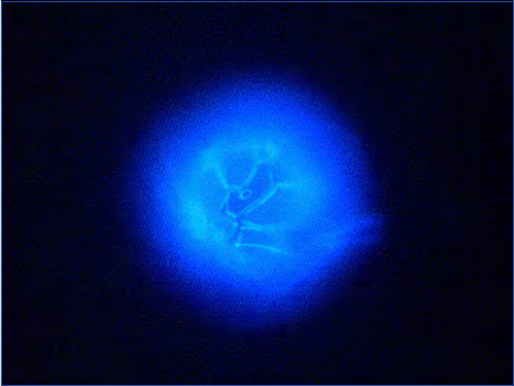
This will give dinoflagellate thecae a clear intensive blue epi-
fluorescence including the sutures of the plates (Fig. 14). Oth-
er cellulose items like chlorophyte cell walls, cell walls of fungi
parasitising in diatoms etc. will also fluoresce.
Note that the intensity of epifluorescence is pH dependent, in
acidic samples epifluorescence is absent or poor.
Discussion
The Utermöhl method for the examination of phytoplankton
communities is probably the most widely used method for
the quantitative analysis of phytoplankton. Through the years
both microscopes and sedimentation chambers have develo-
ped considerably, yet it is the taxonomic skill of the analyst
that sets the standard of the results.
The Utermöhl method determines both the quantity and di-
versity of phytoplankton in water samples. Moreover, with
only a little extra effort, the biovolume of the different species
can also be elucidated. The method allows very detailed anal-
ysis and with high quality lenses the resolution of phytoplank-
ton morphology can be very good. The Utermöhl method has
some disadvantages. It is very time consuming and thus also
very costly. In order to achieve reliable results the analyst has
to be skilled, with a good knowledge of the taxonomic litera-
ture. It is commonly agreed that analysts take some years to
train and must then keep up to date with the literature.
Figure 14. Alexandrium ostenfeldii, epifluorescence light micros-
copy, stained with Fluorescent Brightener. Note the clear indication
of the sutures and the large ventral pore, characteristic for this
species.
IOC Manuals & Guides no 55
Chapter 2 The Utermöhl method
20
References
Andersen P, Throndsen, J (2004) Estimating cell numbers. In Hal-
legraeff, GM, Anderson DM, Cembella AD (eds) Manual on
Harmful Marine Microalgae. Monographs on Oceanographic
Methodology no. 11. p. 99-130. UNESCO Publishing
CEN/TC 230 (2005) Water quality — Guidance on quantitative
and qualitative sampling of marine phytoplankton. pp. 26.
Edler L (1979) Recommendations on methods for Marine Biologi-
cal Studies in the Baltic Sea. Phytoplankton and Chlorophyll. Bal-
tic Marine Biologists Publication No. 5, p 38
Elbrächter, M, 1994. Green autofluorescence – a new taxonomic
feature for living dinoflagellate cysts and vegetative cells. Rev. Pal-
aeobot. Palynol. 84: 101-105.
Fritz, L., Triemer, RE 1985. A rapid simple technique using cal-
cofluor White M2R for the study of dinoflagellate thecal plates. J.
Phycol. 21: 662-664.
Hallegraeff GM, Anderson, DM, Cembella AD (2004) Manual on
Harmful Marine Microalgae. Unesco Publishing, Paris. ISBN 92-
3-103871-0
Hasle GR (1978a) The inverted-microscope method. In: Sournia,
A. (ed.) Phytoplankton manual. UNESCO Monogr. Oceanogr.
Method. 6: 88-96
Hasle GR (1978b) Identification problems. General recommen-
dations. In: Sournia A (ed.):Phytoplankton manual. UNESCO
Monogr. Oceanogr. Method. 6: 125-128
Heimdal BR (1978) Coccolithophorids. In: Sournia A (ed.):
Phytoplankton manual. UNESCO Monogr. Oceanogr. Method.
6: 148-150
HELCOM Combine Manual, 2006. http://www.helcom.fi/Monas/
CombineManual
Lund JWG., Kipling C, Le Cren ED. (1958) The inverted micro-
scope method of estimating algal numbers and the statistical basis
of estimations by counting. Hydrobiologia 11:2, pp. 143-170
Nauwerck A (1963) Die Beziehungen zwischen Zooplankton und
Phytoplankton im See Erken. Symb. Bot. Ups. 17(5): 1-163
Throndsen J (1978) Chapter 4. Preservation and storage. In: Sour-
nia A (ed.): Phytoplankton manual. UNESCO Monogr. Ocea-
nogr. Method. UNESCO. 6: 69-74
Tikkanen T, Willén T (1992) Växtplanktonflora. Naturvårdsverket.
ISBN 91-620-1115-4. pp. 280
Utermöhl H (1931) Neue Wege in der quantitativen Erfassung des
Planktons. (Mit besonderer Berücksichtigun des Ultraplanktons).
Verh. Int. Ver. Theor. angew. Limnol. vol. 5, no. 2. p. 567-596
Utermöhl H (1958) Zur Vervollkommnung der quantitativen
Phytoplankton-Methodik. Mitt int. Verein. theor. angew. Lim-
nol. 9: 1-38
Venrick EL (1978) How many cells to count? In: Sournia A (ed.):
Phytoplankton manual. UNESCO Monogr. Oceanogr. Method.
6: 167-180
Willén E (1976) A simplified method of phytoplankton counting.
British Phycology Journal. 11:265-278
Willén T (1962) Studies on the phytoplankton of some lakes con-
nected with or recently isolated from the Baltic. Oikos. 13: 169-199

21
Microscopic and Molecular Methods for Quantitative Phytoplankton Analysis
Chapter 3 Settlement bottle method
3 Settlement bottle method for quantitative
phytoplankton analysis
Georgina McDermott*
1
and Robin Raine
2
1
Environmental Protection Agency, (Castlebar), Co. Mayo, Ireland
2
Martin Ryan Institute, National University of Ireland, Galway, Ireland
*Author for correspondence: G.McDer[email protected]
Introduction
The settlement bottle technique is a modified Utermöhl tech-
nique (Hasle 1978) for quantifying phytoplankton. It relies
on the observation and enumeration of phytoplankton cells
after sedimentation using an inverted microscope. It differs
from other similar methodologies as once a sample has been
taken and is preserved, there is no further requirement for
any more sub-sampling or manipulation. Once a water sam-
ple has been taken, it is transferred directly into a plastic tis-
sue culture flask, a preservative is added and the sample is
stored until analysis. For counting, the contents of the flask
are gently shaken, allowed to settle onto one of the flat sides
of the flask which is then placed directly onto an inverted
microscope. As with other Utermöhl methods, it requires the
skills of an analyst experienced in the identification of phyto-
plankton cells.
Materials
Laboratory facilities
The settlement bottle method is simple in that all it requires
are tissue culture flasks (acting as sample jars and counting
chambers), some preservative and an inverted microscope.
Thus all that is required is a room, preferably without direct
sunlight, with enough space and a power supply to use an
inverted microscope.
Equipment
Tissue culture bottles of 50-60 mL capacity are used. Larger
volume bottles are difficult to place on a microscope and suf-
fer from movement of water inside them during examination.
Smaller sized bottles will probably not contain enough sam-
ple. The bottles should be rectangular in shape, as opposed to
having a triangular form, as this makes the calculation at the
end much simpler.
The base of the tissue culture bottles are examined using an
inverted microscope. This should be equipped with 10X, 20X
and 40X objective lenses. The 20X and 40X lenses should
have a long focal length. The technique can be applied using a
choice of either brightfield or phase contract microscopy. Dif-
ferential interference contrast (DIC) and epifluorescence mi-
croscopy are unsuitable. A specialised plate for secure mount-
ing of the settlement bottle onto the stage of the inverted
microscope may need to be manufactured. See Appendix for
examples of equipment.
Chemicals and consumables
The only chemicals that are required are solutions of preserva-
tive. Lugol’s iodine, neutral formalin or glutaraldehyde are all
suitable.
Methods
Preparation of sample
Before taking a sample, a tissue culture bottle should be la-
belled with appropriate information (Date, location, station
number, depth) with a permanent marker pen. Labels should
be written on the edge or narrow side of the bottle, not on the
broad side (see Fig. 1) so that it does not interfere with the
identification and enumeration of cells.
The tissue culture bottle should be filled to the top with the
water sample, leaving just enough air space to add preserva-
tive. This prevents the introduction of large air bubbles which
can degrade the optical path when examining through or near
the edge of the bubble.
Before the sample is allowed to settle it should be wiped clean
and acclimated to room temperature for 24 hours and then
gently shaken to disrupt any aggregation of phytoplankton
cells. This can be achieved by a combination of horizontally
rolling and vertically turning the sample bottle upside down
as gently as possible to prevent the break-up of colonies and
the accumulation of air bubbles. The contents of the tissue
culture flask should be allowed to settle for a period of at least
six hours.
Analysis of sample
The phytoplankton cells can then be counted using an in-
verted microscope. The entire base of the bottle or a number
of strips, going across the length or width of the bottle, can be
examined and the cells of each species or type are scored (see
Fig. 2 for details).
Preservation and storage
As with all samples of phytoplankton, deterioration is ex-
tremely fast in direct sunlight. All samples should therefore
be stored in the dark, stacked, preferably horizontally, to
minimise storage space. Samples should also be kept cool, al-
though refrigeration is not absolutely necessary. Storage over
long periods of time (months) is not as effective using Lugol’s
iodine, as opposed to formalin or glutaraldehyde, as leaching
of iodine into the plastic will occur which will deteriorate the
quality of microscopic observations.

IOC Manuals & Guides no 55
Chapter 3 Settlement bottle method
22
Scope
Qualitative and quantitative analysis of phytoplankton.
Detection range
Detection range is dependent on the volume of sample settled
and the number of strips analysed. Counting over the base of
a 50 mL settlement bottle will give a detection limit of ca. 20
cells per Litre.
Advantages
Avoidance of errors arising from sub sampling. Qualitative as
well as quantitative analysis. Identification and quantification
of multiple or single species. Detection of harmful species. Se-
diment bottles are available at low cost.
Drawbacks
Optical resolution is reduced due to the thickness of the wall of
the settlement bottles. This is a time consuming analysis that
requires skilled personnel. Sedimentation time prevents the im-
mediate analysis of samples. DIC and epifluorescence micros-
copy are not suitable with this method. Special long distance
objectives must be used at higher magnifications.
Type of training needed
Analysis requires continuous training over years with in-depth
knowledge of taxonomic literature.
Essential Equipment
Inverted microscope, settlement bottles, identification litera-
ture.
Equipment cost*
Inverted microscope: 7,500 – 50,000 € (11,000 – 70,000 US $).
Identification literature: 1,000 – 3,000 € (1,400 – 4,300 US $).
Consumables, cost per sample**
Less than 5 €/4 US $.
Processing time per sample before analysis
A minimum of 6 hours sedimentation time for a 50 mL sett-
lement bottle.
Analysis time per sample
2-10 hours or more depending on type of sample and analysis.
Sample throughput per person per day
1-4 depending on type of sample and analysis.
No. of samples processed in parallel
One per analyst.
Health and Safety issues
Analysis sitting at the microscope is tiresome for eyes, neck and
shoulder. Frequent breaks are needed. If formalin is used as pre-
servation agent appropriate health and safety guidelines must
be followed.
*service contracts not included
**salaries not included
The fundamentals of
The settlement bottle method
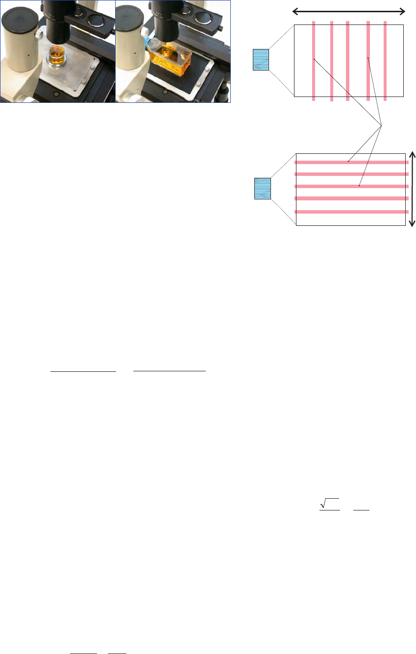
23
Microscopic and Molecular Methods for Quantitative Phytoplankton Analysis
Chapter 3 Settlement bottle method
Calculation of results
Once a count of a particular species or type has been com-
pleted, this must be multiplied by a conversion factor (in
this case F) to calculate the cell density per unit volume. This
type of conversion applies to all sedimentation techniques for
enumerating phytoplankton cells. The general formula for
achieving a value of F to derive the cell density in cells per
Litre is:
The value of F will vary when counting in strips along the
bottle. This will depend on the magnification of the objective
lens, the number of strips across the bottle which were exam-
ined, and whether the strips were oriented along or across the
bottle. The width of the field of view (i.e. the width of each
strip) must be predetermined using a calibrated graticule at
each magnification. If one is scanning the long side of the bot-
tle, the length of the short side across the bottle is required,
and vice versa.
A worked example
A tissue culture bottle of 50 mL capacity was filled with a sea
water sample and preserved with Lugol’s iodine. The content
of the bottle was gently shaken and allowed to settle onto the
flat side of the bottle; dimensions 60 x 30 mm. Five strips
across the long length of this flat side were examined using a
20X objective lens. The width of the field of view was previ-
ously estimated as 0.95 mm at this magnification. A total of
135 cells of Karenia mikimotoi were counted.
In this example five strips across the long side were originally
examined (as shown in Fig. 2b) the value for F then becomes:
Where 30 equals the width of the bottle (mm)
5 equals the number of strips counted
0.95 equals the width of the transect counted (mm)
The density of K. mikimotoi cells in the sample then be-
comes:
135 * 126.3 = 17,000 cells per Litre.
The standard error (SE) using this technique, as a percentage,
is typically the square root of the number of cells counted,
expressed as a proportion of the cells counted:
This gives an overall result of a cell density for K. mikimotoi of
17,000 cells per Litre ± 1,500. Note the number of significant
figures in this result (1,500 has been rounded from 1,467).
Discussion
A common problem in plankton identification and enu-
meration is archiving a particular sample for future reference,
verification of the identity of a species or even accurate inter-
calibration studies. A particular advantage of the settlement
bottle technique is the minimisation of sample handling
which can, at times, introduce serious errors. A sample is di-
Figure 2. Methods of counting strips (shaded areas) across a cell
culture bottle. If, for example, the width of the field of view, and
hence of each strip is 0.95 mm, then the F factor may be calcula-
ted. In a) where the strips are widthways the ratio of total area to
the area counted is 60/(5 * 0.95). In b) with the strips lengthways
this ratio is 30/(5 * 0.5). With a sample volume inside the bottle of
50 mL, the F factor for a) then becomes (60/(5 * 0.95)) * (1000/50)
= 12.6 * 20 = 252. In b) the F factor is (30/(5*0.95))*(1000/50)
= 6.3 * 20 = 126. F factors can become very high using the cell
culture bottle technique unless a suitable number of strips are
counted.
Strips scanned across the
width of the bottle. The width
of the strip is the width of the
field counted. In the example
this is 0.5 mm.
Settlement bottle length 60 mm
Settlement bottle
width 30 mm
a)
b)
Figure 1. A comparison of a) the Utermöhl settlement chamber
and b) the settlement bottle method for counting phytoplankton
cells using an inverted microscope. In the example above a 10
mL settlement chamber shows a similar height of water from
which samples are sedimented as the 50 mL cell culture bottle
used in b), allowing the same density of cells on the base of each.
However, a much bigger surface area can be examined when
using the settlement bottle, allowing more accurate estimations
of, in particular, the larger species since more cells are counted.
This can be done quite rapidly at lower power magnifications, for
example using a X10 objective lens. Note the sample label of sta-
tion number and depth is written on the side of the bottle (date and
location are on the opposite side). Note also that special mounts
on the movable stage are required for both types of settlement
container.
A B
*
Sample volume
1000 (mL)
Settling area
Area analysed
F =
F =
95.0*5
30
*
50
1000
= 126.3
8.6%
135
11.6
135
135
==

IOC Manuals & Guides no 55
Chapter 3 Settlement bottle method
24
rectly put into a tissue culture bottle, preserved and capped in
the field, after which there is no further need for any future
sub-sampling. Samples fixed with formalin can be stored in-
tact for an extended period of time. If noxious chemicals such
as formalin or glutaraldehyde are used as preservatives, then
there is no danger of contamination or fumes resulting from
them as the sample is in an air- and water-tight container.
Additionally, many samples can be prepared for analysis at
any given time as there is no need for an extended range of
relatively expensive settlement chambers.
No technique is without imperfections. In the case of the set-
tlement bottle method the most irritating of these is probably
the leaching of iodine into the sides of the tissue culture bottle
if either acidic or neutral Lugol’s iodine is used to preserve the
samples. This occurs after a few weeks, and reduces the qual-
ity of the observations. As the sample is enclosed, sedimented
specimens of phytoplankton cannot be manipulated which
can on occasion make identification very difficult. Observa-
tions of cells at the extreme edges sides of the bottle can be
difficult. However, the method is ideal for long-term storage
especially if the samples are stored with formalin. The method
is also very low cost relative to other techniques.
Acknowledgements
One of the authors (GMcD) wishes to acknowledge the fi-
nancial assistance of Bord Iascaigh Mhara for attendance at
the WKNCT workshop in Kristineberg, Sweden.
References
Hasle GR (1978) Counting phytoplankton cells In Sournia A (ed.)
Phytoplankton Manual. UNESCO, Paris, p337.
Equipment Supplier and model reference € US $
Inverted Microscope e.g. Nikon TS100F, Olympus CKX41 5,000-6000
†
6,500-8,500
Tissue Culture Bottles Any medical laboratory supplier 0.5-1 each Ca. 1 each
Table 1. Equipment and suppliers.
Appendix
†
The price can vary considerably depending on the quality of the objective lenses used. The price here
is for a reasonable quality set of 10X, 20X and 40X lenses.

25
Microscopic and Molecular Methods for Quantitative Phytoplankton Analysis
Chapter 4 Counting chamber methods - Haemocytometer, Palmer-Maloney cell and Sedgewick-Rafter cell
General introduction
The counting chamber methods are established methods
to count phytoplankton. The three most common types of
counting chambers for phytoplankton enumeration are the
Sedgewick-Rafter counting slide, the Palmer-Maloney coun-
ting slide and the haemocytometer counting slide. All three
methods are easy to learn and use, requiring preserved sample,
a good quality compound microscope and counting slides.
The set up cost is low and it is beneficial to have a selec-
tion of all three on hand in the laboratory. These methods are
particularly suitable for samples containing a high concentra-
tion of cells, as in bloom situations or in phytoplankton cul-
tures with the haemocytometer being reserved for extremely
high cell densities of small organisms. The capability of the
Sedgewick-Rafter and the Palmer-Maloney to view the whole
phytoplankton community including the presence of harmful
species is a definite asset. Nevertheless correct identification
of the phytoplankton community still requires highly trained
analysts for its implementation.
Sedgewick-Rafter counting slide
Introduction
The Sedgewick-Rafter counting slide is a traditional counting
method using a compound microscope and a highly trained
taxonomist. This is a rapid method for quantifying samples
with high cell numbers. The slide is comprised of a transpa-
rent base, which has a centrally mounted chamber (50 mm
x 20 mm x 1 mm deep) and can hold 1 mL of sample. The
base of this chamber has a ruled 1 mm grid, so that the 1 mL
sample is subdivided into single microlitres. This chamber is
covered over by a cover glass, which protects the sample from
drying out and disturbances by air currents. The sample is
then counted using a compound microscope.
Materials
Equipment
• A standard, compound microscope with 10X and 20X
objectives and brightfield and phase contrast. A 40X ob-
jective may not be able to be used for this analysis, this
depends on the working distance of the objective lenses.
• A Sedgewick-Rafter slide: This can be made from plastic
or glass.
• A tally counter is useful when counting high cell num-
bers.
4 Counting chamber methods for quantitative phytoplankton
analysis - haemocytometer, Palmer-Maloney cell and
Sedgewick-Rafter cell
Murielle LeGresley*
1
and Georgina McDermott
2
1
Fisheries & Oceans Canada, Biological Station, 531 Brandy Cove Road, St. Andrews, NB E5B 2L9, Canada
2
Environmental Protection Agency, John Moore Road, Castlebar, Co. Mayo, Ireland
*Author for correspondence e-mail: Murielle.LeGresley@dfo-mpo.gc.ca
Chemicals and consumables
• A pipette is needed to dispense the sample into the cell.
• Sample bottles for storing the samples.
Solutions for preservation
• Lugol’s iodine or formalin.
Methods
1 Prior to analysis the sample should first be homogenised.
This is achieved using a combination of horizontally rol-
ling and vertically turning the sample bottle as gently as
possible to prevent the breakup of colonies and the ac-
cumulation of bubbles;
2 From a well mixed sample, 1 mL is removed using a pi-
pette. The pipette should have a wide opening that does
not restrict the movement of larger phytoplankton spe-
cies (such as Noctiluca scintillans, Ceratium species). This
is especially important when using a 1 mL pipette with
removable tips, the end of the tip should be cut off to
widen the opening;
3 The cover glass should be placed carefully onto the coun-
ting slide, perpendicular to the long axis of the slide, so
one corner is left open for filling and another for the es-
cape of air;
4 The sample aliquot is then dispensed into the counting
cell (Fig. 1a – f):
5 Slowly swing the cover glass so that it completely covers
the sample. Careful alignment of the cover glass will pre-
vent air bubbles from being introduced into the sample
and will ensure that the sample holds its complete vo-
lume. If a bubble develops, refill the counting cell.
6 Preserved samples should be left to settle for 15 minutes
before enumeration;
7 The sample is then examined using a compound micros-
cope. The slide should first be scanned under low mag-
nification to estimate the concentration of cells. Using
this information a counting strategy is decided upon as
to whether the whole slide or a noted fraction is to be
counted;
8 If the concentration of phytoplankton in the Sedgewick-
Rafter slide is too dense and the cells are overlapping thus
hindering identification, a dilution step should be perfor-
med using filtered seawater for marine samples;
9 After analysis is completed the slide is washed and clea-
ned between samples to prevent cross-contamination. A
pure detergent like soap is recommended (Hallegraeff et
al. 2004);

IOC Manuals & Guides no 55
Chapter 4 Counting chamber methods - Haemocytometer, Palmer-Maloney cell and Sedgewick-Rafter cell
26
The fundamentals of
The counting chamber methods
Counting chamber Sedgewick-Rafter Palmer-Maloney Haemocytometer
Scope
Cultures and high cell numbers Cultures and high cell densities as in bloom
conditions
Cultures and extremely high cell concentration of
small organisms
Detection range
1,000 cells L
-1
Limit of Detection (LOD) 10,000 cells L
-1
(LOD) 10,000,000 cells L
-1
(LOD)
Advantages
A rapid estimate of cell concentrations A rapid estimate of high cell concentrations A rapid estimate of extremely high cell
concentrations
Drawbacks
Accurate results only when sample contains high
phytoplankton cell densities
Accurate results only when sample contains very
high cell densities
Accurate results only when sample contains
extremely high cell densities
Type of training needed
Method-easy to learn and use.
Highly trained taxonomist needed for verication of
species identication
Method-easy to learn and use.
Highly trained taxonomist needed for verication
of species identication.
Method-easy to learn and use.
Highly trained taxonomist needed for verication of
species identication
Essential Equipment
Compound Microscope
Cover slips
Pipettes
Compound Microscope
Cover slips
Pipettes
Compound Microscope
Pipettes
Sedgewick-Rafter slides Palmer Maloney slides Haemocytometer slide with cover glass
Equipment cost
Compound Microscope: € 2500 / 3250 US $ Compound Microscope: € 2500 / 3250 US $ Compound Microscope: € 2500 / 3250 US $
Sedgewick-Rafter slides:
Perspex :€50/ 65 US $
Glass: €166/ 213 US $
Palmer-Maloney slides:
Ceramic- €60/ 80 US $
Stainless Steel-€170/$230 US $
Haemocytometer slide:
€200/ 230 US $
Consumables, cost per sample
€ 1/$1.3 US $ € 1/$1.3 US $ € 1/$1.3 US $
Processing time/sample:
20 minutes 5 minutes 5 minutes
Analysis time /sample:
This depends on the sample density 10-30 min/ sample depending on the sample
density
< 20 min / sample depending on the sample density
Sample/throughput/person/ day
This depends on the sample density 14-20 dependent on target species and density of
samples
< 30 dependent on target species
Samples processed in parallel
Only one sample at a time Only one sample at a time Only one sample at a time
Health and Safety issues
Dependent on preservative used Dependent on preservative used Dependent on preservative used
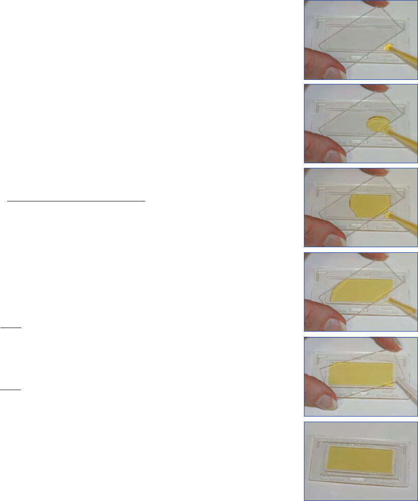
27
Microscopic and Molecular Methods for Quantitative Phytoplankton Analysis
Chapter 4 Counting chamber methods - Haemocytometer, Palmer-Maloney cell and Sedgewick-Rafter cell
Preservation and storage
Samples should be stored in the dark (closed boxes) to avoid
direct light (which affects the Lugol’s iodine preservative) and
at room temperature. Samples preserved with Lugol’s iodine
can deteriorate over time resulting in a paler solution which
could impare preservation. If the samples are stored for ex-
tended periods, preservation should be checked regularly and
further Lugol’s iodine added as appropriate.
Formulas for calculating results
The Sedgewick-Rafter slide has a volume of 1 mL with the
base of the cell being divided into 1,000 squares (50 rows
by 20 rows), each representing 1/1,000 of the volume of the
slide.
To obtain a final result expressed as cells L
-1
, the following
equation is used to calculate the multiplication factor (F). F
is dependent on the number of squares of the base of the cell
counted during the analysis.
Examples of F for the Sedgewick-Rafter slide:
4 rows (200 squares) are counted.
50 rows (1000 squares) or the entire slide is counted.
Discussion
The Sedgewick-Rafter slide is best used when analysing cul-
tures or high biomass blooms. As this method does not re-
quire an overnight settling period, it is rapid and can provide
a quick assessment of a water sample. It has been proven to
provide accurate results between 10,000 (ICES 2006) and
100,000 cells L
-1
(McAlice 1971). The set up cost is low due
to the use of a compound microscope.
The Sedgewick-Rafter slide tends to perform better with
samples containing larger phytoplankton cells. Another coun-
ting method may have to be used for samples with low cell
densities. It may be possible to pre-concentrate cells using a
filtering/settling step when the target organism is present in
low concentrations.
Plastic Sedgewick-Rafter slides tend to scratch easily and care
must be taken when cleaning the cell. Scratches may hinder
the accurate identification of cells. Due to the design of the
Sedgewick-Rafter slide it may be difficult to use the 40X mag-
nification. This could prove a problem in the identification of
smaller (10-15 µm) phytoplankton cells. In addition exteme
care must be taken to load the Sedgewick-Rafter slide cor-
rectly and avoid the introduction of air bubbles to ensure the
even distribution of phytoplankton in the slide.
000,1*
000,1
countedSquaresofNumber
F =
000,5000,1*5000,1*
200
000,1
===F
000,1000,1*1000,1*
000,1
000,1
===F
Figure 1. A – F: Loading Lugol’s iodine preserved sample into
Sedgewick-Rafter cell.
A
B
C
D
E
F
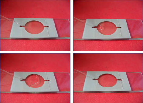
IOC Manuals & Guides no 55
Chapter 4 Counting chamber methods - Haemocytometer, Palmer-Maloney cell and Sedgewick-Rafter cell
28
Palmer-Maloney counting slide
Introduction
The Palmer-Maloney counting slide method is a rapid and
straightforward technique that was first employed to enume-
rate nanoplankton. The counting chamber is round, measures
17.9 mm in diameter, 400 µm depth and holds a volume 0.1
mL of sample. Two loading channels are located on either
side of the counting slide (Fig. 2 a-d). The Palmer-Maloney
slide does not have any rulings or grid. This counting slide is
useful with cultures, samples with high cell densities or pre-
concentrated samples. The detection level is 10,000 cells L
-1
or 10 cells mL
-1
(Guillard 1978).
Equipment
A standard compound microscope or an inverted microscope
with 10X and 20X objectives. Phase contrast and epifluores-
cence capability are valuable asset to the identification of phy-
toplankton.
• Palmer-Maloney counting slide
• Cover glass (22mm X 22mm or 50mm X 22 mm)
• Pipettes (Pasteur or disposable) needed to dispense the
sample
• A tally counter is useful when counting high cell num-
bers
Chemicals and consumables
• Preservative (Lugol’s iodine, Formalin) (see chapter 2 for
recipes)
• Alcohol for cleaning slides
Method
1 The cover glass should initially be placed over the coun-
ting chamber;
2 The preserved sample should be inverted gently about
10-20 times to ensure homogenisation. A pipette is filled
with the well-mixed sample;
3 The chamber of the counting slide is then filled by gradu-
ally dispensing an aliquot of sample from the pipette into
one of the loading channels (Fig. 2 a-d). It is important
that no air bubbles are present in the chamber. Trapped
air may be removed by slowly sliding the cover slip back
then replacing it in its original position however it may
be nessecary to repeat steps 1-3;
4 The slide should be left to settle for 5 minutes;
5 Counting organisms should begin at the top or bottom
edge and continue until all area of the chamber is exa-
mined excluding loading channels. The centre of the lo-
ading channels are effective reference points to count half
of the slide;
6 Once the count has been completed the slide and cover
glass should be rinsed thoroughly with water then with
alcohol and wiped clean with lint-free wipes.
Preservation and storage
Any preserved samples can be used with this method.
Note: samples preserved in Lugol’s iodine- should be kept in
the dark and checked periodically for light tea colour, adding
more preservative if needed.
Formulas for calculating results
Since the volume of a Palmer-Maloney slide is 0.1 mL, mul-
tiply the total count by 10,000 to obtain the number of
cells L
-1
.
For example:
Cells per Litre= total cell count * 10,000
Final count in the Palmer-Maloney slide is 200 cells; 200 *
10,000= 2,000,000 cells L
-1
Discussion
The Palmer-Maloney counting slide method is excellent to
enumerate dense blooms, net tows, cultures or pre-concentra-
ted samples. It is an inexpensive and rapid counting method
in which the entire phytoplankton community may be obser-
ved including harmful algae species.
This counting slide is appropriate for enumerating most spe-
cies but is not as useful for counting large organisms (>150
µm) or long chain-forming diatoms as these may not be dist-
ributed evenly in the sample (Guillard and Sieracki 2005).
Because of the thickness of the Palmer-Maloney slide the hig-
hest magnification objective lenses possible to use with some
compound microscopes is 10X or 20X. Thus this slide is not
a good choice when the proper identification or enumeration
of an organism requires a higher magnification. This can be
addressed by using an inverted microscope with a higher ob-
jective. The Palmer-Maloney slide may also be used with cal-
cofluor stain and an epifluorescence microscope for thecate
dinoflagellate identification.
When using the small cover slips (22 mm x 22 mm) the sam-
ple may have a tendency to evaporate. This problem can be
solved by using longer cover slips (22 mm x 55 mm) or by
applying parafilm to cover the loading channels. This method
may be used to monitor target species that are deemed to be
harmful only at very high cell concentrations.
Figure 2 A –D: Loading sample into the Palmer Maloney cell
A B
C D
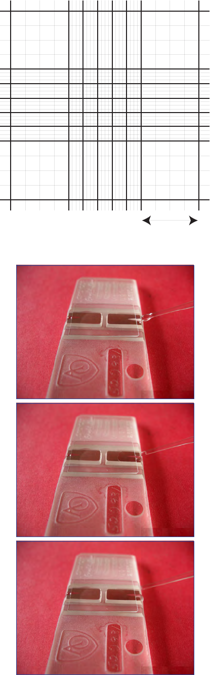
29
Microscopic and Molecular Methods for Quantitative Phytoplankton Analysis
Chapter 4 Counting chamber methods - Haemocytometer, Palmer-Maloney cell and Sedgewick-Rafter cell
Haemocytometer counting method
Introduction
The haemocytometer (also used for counting blood cells) is a
counting slide method specially practical for cultures and ex-
tremely high concentrations of cells of small sized organisms
(< 30 µm). The middle of the slide has the appearance of an
“H” which separates the 2 thin silver-coloured chambers both
engraved with a nine-square grid. Haemocytometers may be
purchased in either 0.1 mm or 0.2 mm depth and may possess
different grid subdivisions. The most common slide of this
type is 0.1 mm deep with Improved Neubauer ruling (Fig.
3); each chamber holding nine 1-mm large squares separated
by double or triple rulings. The volume in nine large squares
is 0.0009 mL, with the 2 chambers having 18 squares with a
total volume of 0.0018 mL.
Equipment
• A standard compound microscope or an inverted micros-
cope with 10X and 20X objectives, phase contrast
• Haemocytometer counting slide (Improved Neubauer
rulings)
• Cover glass supplied with haemacytometer
• Pipettes (Pasteur)
Chemicals and consumables
• Preservative (Lugol’s iodine, Formalin) ( see chapter 2 for
recipes)
• Alcohol for cleaning slides
Methods
1 A cover glass is placed over both chambers of the haemo-
cytometer;
2 With a soft undulating motion, the preserved sample is
gently inverted appoximately 10-20 times to ensure the
sample is mixed thoroughly;
3 A Pasteur pipette is filled with the well-mixed sample;
4 Each chamber of the haemocytometer is loaded by hol-
ding pipette at a 30 to 45 degree angle with the open
dispensing tip in the V-shaped slash, allowing the pipette
tip to touch the slot then slowly expelling a drop of the
liquid. The capillary action will fill the chamber with the
sample. It is important to check that the liquid spreads
over the silver- coloured chamber without overflowing
into the moats. (Fig 4);
5 Step 2-4 is repeated to fill the other side of the chamber.
Allow 2-3 minutes for cells to settle;
6 The slide should be scanned initially in the microscope to
determine the counting strategy. The whole slide or a se-
lected number of large squares should be counted to ob-
tain a statistically significant number of cells (Andersen
and Throndsen 2004). Each side of the haemocytometer
slide has a grid with nine large 1 mm
2
squares which are
further subdivided depending on the type of haemocyto-
meter;
Figure 3. Drawing of haemocytometer with improved Neubauer ruling.
Figure 4 A-C: Loading sample into haemocytometer.
1 mm
A
B
C

IOC Manuals & Guides no 55
Chapter 4 Counting chamber methods - Haemocytometer, Palmer-Maloney cell and Sedgewick-Rafter cell
30
7 The number of organisms and the number of squares
counted should both be noted. To avoid counting cells
twice, it must be determined beforehand to include cells
that touch 2 of the 4 sides of each square (i.e. the top and
left side of each large square while ignoring the cells that
touch the bottom and right side);
8 After the count has been completed the haemocytometer
slide must be cleaned thoroughly by rinsing the slide and
cover glass with running water then with alcohol, wiping
clean with lint-free wipes.
Preservation and storage
Any preserved samples can be used.
Note: samples preserved in Lugol’s iodine- should be kept in
the dark and checked periodically for light tea colour, adding
more preservative if needed.
Formulas for calculating results
Total the cells and divide by the number of large 1 mm squa-
res counted to obtain the average number of cells per square.
Multiply this average cell number by 10,000 to obtain num-
ber of cells per mL. (Alternately to obtain the number of
cells per Litre, multiply the average number of cells per large
square by 10,000,000).
The average number of cells per mL = average count per large
square X 10,000
For example: In total 200 cells in 4 large squares are counted:
Discussion
The haemocytometer counting method is excellent for coun-
ting cultures or an extremely high concentration of small cells.
The slide can be used with 10X objective with the compound
microscope or with 10X or 20X objectives with an inverted
microscope. This method is not suitable for routine water
monitoring because of the high cell biomass needed to get
statistically significant numbers. It will not give an overview
of the whole phytoplankton community especially organisms
with a low cell density. It is not compatible with large orga-
nisms because of the shallow 0.1 mm depth of the slide. It is
better to use the slide for extremely high cell estimates.
Pre-concentration of sample
Concentration of sample may be necessary when cell density
is low. This can be achieved using a settlement method where
a sample is poured into a graduated cylinder (of volume (A))
and allowed sufficient time for cells to settle (one hour for
each cm height of cylinder or overnight). After settling, the
water from the upper portion of the sample is gently removed
and the final volume (B) noted. Another method involves fil-
tering the sample through a 10 or 20 µm mesh (i.e. plankton
net). The concentration factor (CF) is calculated by dividing
the initial volume (A) by the final volume (B). The remain-
ing volume should be mixed well and the instructions of the
counting method followed, remembering to divide the total
cell count by the CF.
Example:
The original volume (A) = 100 mL
Final volume (B) = 10 mL
Acknowledgements
One of the authors (GMcD) wishes to acknowledge the as-
sistance of Bord Iascaigh Mhara (The Irish Fisheries Board).
for assistance in attending the WKNCT workshop in Kris-
tineberg, Sweden.
References
Andersen P, Throndsen J (2004) Estimating cell numbers. In: Halle-
graeff GM, Anderson DM, Cembella AD (eds) Manual on Harm-
ful Marine Microalgae 99-129
Guillard RRL (1978) Counting Slides. In: A. Sournia (ed) Phyto-
plankton Manual. UNESCO Publishing 182-189
Guillard RRL, Sieracki MS (2005) Counting cells in cultures with
the light microscope. In: Andersen RA (ed) Algal Culturing
Techniques Elsevier Academic Press 239-252
Hallegraeff GM, Anderson DM, Cembella AD (2004) Manual on
Harmful Marine Microalgae. UNESCO Publishing 793pp
ICES (2006) Report on the ICES/IOC workshop on new and clas-
sic techniques for the determination of numerical abundance and
biovolume of HAB species – evaluation of the cost, time-effi-
ciency and intercalibration methods (WKNCT), 22-27 August
2005, Krinstineberg, Sweden. ICES CM 2005/C:10
McAlice BJ (1971) Phytoplankton sampling with the Sedgewick-
Rafter cell. Limnol Oceanogr 16(1)19-28.
10
10
100
===
B
A
CF
50
4
200
==countedcellsofnumberAverage
1
000,500000,10*50
−
mLcellsmL perCells

31
Microscopic and Molecular Methods for Quantitative Phytoplankton Analysis
Chapter 5 Filtering - Calcofluor staining - quantitative epifluorescence microscopy
Materials
Laboratory facilities
The method can be used in a basic laboratory. No special fa-
cilities are required.
Equipment
A filtration unit and a vacuum pump as well as an epifluores-
cence microscope equipped with a mercury lamp and filter set
for DAPI (UV excitation (330-380 nm), emission filter (420
nm) is required, see Table 1.
Chemicals and consumables
The stain, Calcofluor White M2R (Polysciences, Warrington
PA) is especially useful for qualitative as well as quantitative
analysis of thecate dinoflagellates because it stains the cellulose
in the thecal plates of dinoflagellates and not other plankton
organisms or detritus.
Calcofluor White M2R is a fluorescent brighter. The chemi-
cal formula of Calcofluor White M2R is: C
40
H
42
N
12
O
10
S
2
Na
2
.
Calcofluor White M2R can be stored at room temperature.
Method
How to make the Calcofluor working solution
Add approximatley 2 µg Calcofluor to 10 mL of distilled wa-
ter in a clean acid rinsed (5% HCl) glass bottle. The Cal-
cofluor will dissolve immediately, and the working solution
is ready to use. If the glass bottle is not completely clean the
Calcofluor may precipitate and the solution can not be used.
The working solution of Calcofluor does not require preser-
vation. It can remain viable for a few days to several weeks at
room temperature in the laboratory.
Introduction
Identification and enumeration of thecate dinoflagella-
tes, which include several toxic species, is frequently a time
consuming exercise. Species from the genera Dinophysis and
Prorocentrum (the causative organisms of diarrhetic shellfish
poisoning, DSP), Alexandrium and Pyrodinium (the causative
organisms of paralytic shellfish poisoning, PSP), Ostreopsis
and Gambierdiscus (responsible for ciguatera fish poisoning,
CFP) may cause problems to the aquaculture and fishing
industries even when they occur in low concentrations. Tra-
ditionally, quantitative analysis of phytoplankton samples is
performed using the well established Utermöhl sedimenta-
tion procedure (Utermöhl 1958). The Utermöhl procedure
involves sedimentation of the plankton sample (5-50 mL) for
a period of 8 -24 hours depending on the sample volume.
The long sample sedimentation time prior to analysis and the
complexities of identification of thecate dinoflagellates means
that this method cannot provide a rapid result. Quantitative
epifluorescence techniques, basically adapted from the acri-
dine orange technique by Hobbie et al. (1977), involves filtra-
tion and staining of the organisms on polycarbonate filters.
This method, which was originally described for counting of
pelagic bacteria has been modified for counting of hetero- and
autotrophic nanoflagellates as well as larger phytoplankton
and protozooplankton organisms (see e.g. Haas 1982, An-
dersen and Sørensen 1986). Examples of fluorochromes used
are acridine orange (Andersen and Sørensen 1986) or DAPI
(Porter and Feig 1980). Apart from the DNA, these fluoro-
chromes also stain other compounds found in cells. When
working in coastal waters and shallow fjords where the pelagic
biomass is high and often dominated by diatoms, quantifica-
tion of thecate dinoflagellates present in low concentrations
must be carried out on relative large water samples (50-100
mL). In such cases the analysis can be rendered practically im-
possible using either acridine orange or DAPI. This is because
thecate dinoflagellates must be identified among high con-
centrations of other organisms such as diatoms, which also
fluorescence heavily.
In this chapter, a method is presented which is based upon
the quantitative epifluorescence technique using Calcoflour
White M2R as a stain. The method has previously been des-
cribed in Andersen (1995), Andersen and Kristensen (1995),
Andersen and Throndsen (2004). Calcofluor is a specific stain
for the cellulose in the thecal plates of the thecate dinoflagel-
lates (Lawrence and Triemer 1985). The stain does not stain
structures in most other pelagic organisms including the dia-
toms. Using this method it is possible to analyse sample volu-
mes from 10 to 500 mL, thereby obtaining reliable estimates
of thecate dinoflagellates present in low concentrations in the
presence of large concentrations of diatoms.
5 Filtering – calcofluor staining – quantitative epifluorescence
microscopy for phytoplankton analysis
Per Andersen*
Orbicon A/S, Johs. Ewalds Vej 42-44, DK-8230 Åbyhøj, DENMARK
*Author for correspondence e-mail: [email protected]
• Calcofluor White M2R or a similar product
• A 10 mL glass bottle
• Polycarbonate membrane filters (pore size 5 µm)
• Paraffin oil
• Neutral Lugol’s iodine
• A filtration unit
• A vacuum pump
• Glass microscope slides
• Cover slips (24x24 mm)
• An epifluorescence microscope equipped with a mercury
lamp and filter set for DAPI (UV excitation, 330-380 nm,
emission filter, 420 nm)
Table 1. Equipment and consumables required for the quantitative
epifluorescence method using Calcofluor White M2R.

IOC Manuals & Guides no 55
Chapter 5 Filtering - Calcofluor staining - quantitative epifluorescence microscopy
32
Scope
Qualitative and quantitative analysis of thecate dinoflagellates.
Detection range
Detection range is dependent on the volume of sample filtered.
Counting all of the cells from a 200 mL sample will give a de-
tection limit of 5 cells per Litre.
Advantages
Preparation time is short. Specific identification of thecate di-
noflagellates is feasible as the staining makes the relevant morp-
hological features visible. Preparations can be stored for analysis
or re-examination for weeks/months.
Drawbacks
This method is limited to analysis of thecate dinoflagelllates
only. This means that other methods will have to be used if
the rest of the phytoplankton community needs to be studied.
Type of training needed
A basic knowledge of light and epifluorescence microscopy is
needed. Analysis requires continuous training over years with
in-depth knowledge of taxonomic literature.
Essential Equipment
Epifluorescence microscope with UV excitation
Filtration unit incl. pump.
Equipment cost*
20000-50000 US$ (see Appendix to this chapter for details).
Consumables, cost per sample**
Less than 1-2 €/$1-2.
Processing time per sample before analysis
App. 15 minutes for filtration and mounting of filter.
Analysis time per sample
Depending on the number of species to be quantified and vo-
lume filtered. A routine analysis of 5-10 species requires ap-
prox. 15 min. per sample, excl. reporting/database handling of
results.
Sample throughput per person per day
10-20.
No. of samples processed in parallel
One per analyst.
Health and Safety issues
Analysis sitting at the microscope is tiresome for eyes, neck and
shoulder. Frequent breaks are needed. The stain Calcoflour is
for laboratory use only. Caution: Avoid contact and inhalation!
The relevant health and safety guidelines should be followed.
*service contracts not included
**salaries not included
The fundamentals of
The filtering - calcofluor staining - quantitative fluorescence microscopy

33
Microscopic and Molecular Methods for Quantitative Phytoplankton Analysis
Chapter 5 Filtering - Calcofluor staining - quantitative epifluorescence microscopy
Sample preparation
A known volume of sample, fixed using neutral Lugol’s iodi-
ne, is vacuum filtered using a polycarbonate filter with a pore
size 5 µm (Fig. 1). Filters with larger or smaller pore sizes can
be used depending upon the organisms of interest.
When approximatley 1 mL of sample is left in the filter chim-
ney, 0.2 mL (3-4 drops) of Calcofluor White M2R working
solution is added and filtration is continued until the filter is
dry (Table 2).
Note that Calcofluor White M2R will only work at a neutral
pH (= 7). In more acidic samples Calcofluor will precipitate
which will interfere with the identificaiton and enumera-
tion of dinoflagellate cells. If the sample is fixed using acidic
Lugol’s iodine, the sample must be neutralised prior to the ad-
dition of the Calcofluor. To achieve this, the filtration should
be stopped when there is approximatley 0.5 mL of sample left
in the filtration chimney. The filter should then be washed by
adding approx. 2-5 mL of filtered seawater fixed in neutral
Lugol’s iodine. The filtration procedure is then continued as
described as described in Table 3.
The dry filter should be mounted on top of a drop of paraffin
oil on a microscope slide. Another drop of paraffin oil is then
placed on top of the filter and a cover glass is mounted on
top of the paraffin oil (Fig. 2). The filter can then be analysed
using epifluorescence microscopy, using UV excitation (330-
380 nm) and an appropriate emission filter (420 nm). For
routine use an OLYMPUS BH-2 microscope equipped with
a mercury lamp (100 W) or a similar microscope is appro-
priate.
Thecate dinoflagellates can be identified and enumerated,
either by counting the whole surface of the filter or selected
fractions of the filter surface. Large organisms (diameter >20
µm) such as cells from the genus Dinophysis, Prorocentrum
or Alexandrium, can be counted using 100X magnification.
Higher magnifications can be used when it is necessary to see
the morphology of the thecal plates to allow identification to
species level.
The prepared slides for quantitative analysis can be stored in
a refrigerator (< 5
º
C) for weeks with no/very little loss of cells
or fluorescence.
Trouble shooting
The most frequent problems encountered when working with
the quantitative Calcofluor method are:
1 The filter set on the epifluorescence microscope does not
work with Calcofluor White M2R;
2 The pH of the sample to be analysed is not 7;
3 The working solution of Calcofluor has precipitated and the
solution looks milky.
Preservation and storage
Samples to be analysed with this method should preferably
be fixed using neutral Lugol’s iodine. If samples are to be sto-
red for more then a few days the samples should be stored in
brown glass bottles and stored in the dark. Samples stored
according to these guidelines can be kept for months/years,
however, it must be ensured that there is sufficient neutral
Lugol’s iodine in the sample to maintain the perservation.
If the sample has the colour of weak tea there is sufficient
Lugol’s present. If the sample is clear, more neutral Lugol’s
iodine must be added.
Counting procedure and calculation of concen-
trations
Initial analysis of the sample can be performed using a low
magnification such as 100X. The performance of the Cal-
Figure. 1. The filtration equipment used to concentrate phytoplank-
ton on polycarbonate membrane filters for quantification using
epifluorescence microscopy.
Figure. 2. How to mount the polycarbonate filter on a slide for
observation using epifluorescence microscopy.
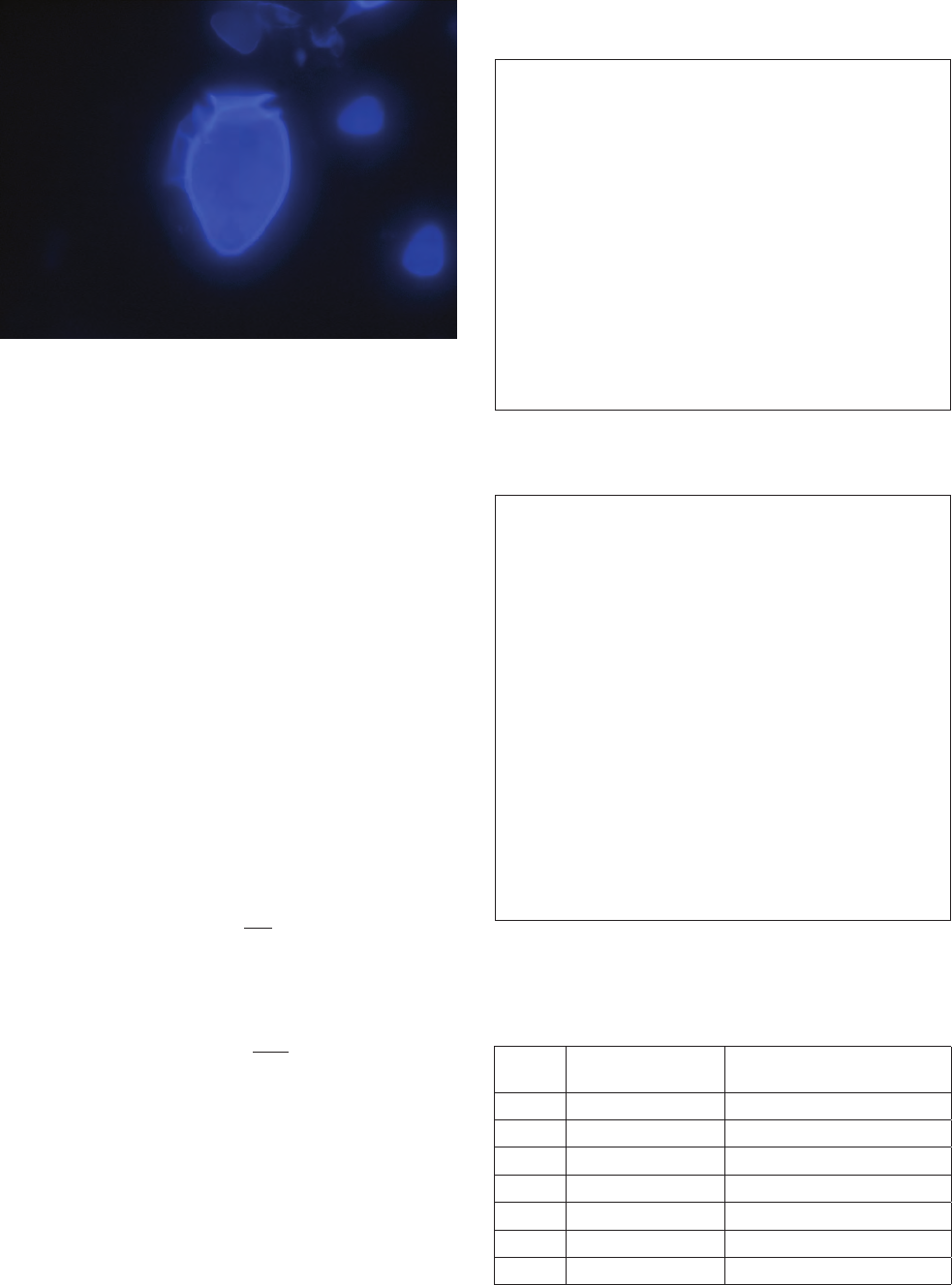
IOC Manuals & Guides no 55
Chapter 5 Filtering - Calcofluor staining - quantitative epifluorescence microscopy
34
cofluor stain must first be assessed by establishing that the
thecate dinoflagellates light up blue on a dark background.
After this has been checked, the sample analysis can be per-
formed.
The counting strategy employed depends on the number of
cells on the filter. It is preferable to count the entire surface of
the filter. If there are a high number of cells on the filter, sub-
sampling or counting only a fraction of the filter (half of the
filter surface or diagonals), can be performed.
Calculation of cell concentrations:
To calculate the concentration (cells L
-1
) of the different spe-
cies in your preparation you must know:
V = Volume of sample concentrated on the filter (mL).
B
a
= Area of the filter (mm
2
).
B
c
= Area of the part of the filter counted (mm
2
).
N = Number of cells counted for the species of interest.
The conversion factor (CF):
The concentration of the species C (cells mL
-1
) is then:
The conversion factors must be calculated for each filtering
unit and microscope as well as for each combination of sub-
sampling area and magnification (Table 4).
Examples of calculations of concentrations using the conver-
sion table are presented in Table 5.
1. Measure the required sample volume using a graduated
cylinder;
2. Add the sample to the filtration unit;
3. Turn on the vacuum pump (maximum pressure = 200
mmHg);
4. Turn off the vacuum pump when there is approximately 1
mL left in the filtration chimney;
5. Add 3-5 drops of CalcoFluor working solution (concentra-
tion 2 mg L
-1
);
6. Turn the vacuum pump on again and filter until the filter
goes dry;
7. Remove the filter from the chimney and dry the back of it
gently on a tissue to remove surplus water;
8. Mount the filter on a drop of paraffin oil on a slide, add
another drop of paraffin oil on top of the filter and put on the
cover slip (24 x 24mm);
9. Observe your preparation using an epifluorescence micros-
cope.
Figure 3. Dinophysis sp. stained with calcofluor as seen in the epi-
fluorescence microscope. The cell height is approximately 50 µm.
1. Measure the required sample volume using a graduated
cylinder;
2. Add the sample to the filtration unit;
3. Turn on the vacuum pump (maximum pressure = 200
mmHg);
4. Stop the filtration when there is about 1-0.5 mL left in the
chimney;
5. Wash the filter by adding approx. 2-5 mL of filtered seawa-
ter fixed in neutral Lugol’s iodine and turn on the vacuum
pump;
6. Turn off the vacuum pump when there is approximatley 1
mL left in the filtration chimney and add 3-4 drops of the
Calcofluor working solution (concentration 2 mg L
-1
);
7. Turn on the vacuum pump again and filter until the filter
goes dry;
8. Remove the filter from the chimney and dry the back of it
gently on a tissue to remove surplus water;
8. Mount the filter on a drop of paraffin oil on a slide, add
another drop of paraffin oil on top of the filter and put on the
cover slip (24x24mm);
9. Observe your preparation using an epifluorescence micros-
cope.
Table 3. Summary of how to prepare samples preserved with
acidic Lugol’s iodine, formaldehyde or gluteraldehyde for the
quantitative epifluorescence method using Calcofluor White M2R.
V
CF
NC *=
Table 2. Summary of how to prepare samples preserved with
neutral Lugol’s iodine for the quantitative epifluorescence method
using Calcofluor White M2R.
Table 4. Example of a calibration table used for calculating con-
centrations of microalgae using epifluorescence microscopy (filter
area = 189 mm
2
. Note: CF is the conversion factor to be applied
when the count of cells in e.g. one diagonal window is to be cal-
culated to the concentration on the total filter surface.
Magni-
fication
Window count
Window area (mm
2
)
Diagonal window count
Diagonal window area (mm
2
)
40X 4.08 31.52
100X 0.66 12.64
200X 0.16 6.2
CF: window CF: diagonal window
40X 46.3 6.04
100X 286 15.1
200X 1181 30.5
c
a
B
B
CF =

35
Microscopic and Molecular Methods for Quantitative Phytoplankton Analysis
Chapter 5 Filtering - Calcofluor staining - quantitative epifluorescence microscopy
Discussion
The method described is excellent for the rapid processing of
samples, for example as required in many toxic phytoplank-
ton monitoring programmes. Low concentrations of thecate
dinoflagellates are easily detected in the presence of high pe-
lagic biomass (e.g. diatoms). This is particularly relevant for
concentrated net tow samples. It is possible to identify thecate
dinoflagellates to species level because of the easy recognition
of the thecal plates of taxonomical importance which can not
always be recognised using the Utermöhl procedure using
Lugol’s iodine preservation.
Samples preserved with neutral Lugol’s iodine produce excel-
lent slide preparations. There is no requirement to use more
toxic preservatives like formaldehyde or glutaraldehyde. The
fluorochrome Calcoflour White MR2 is considered to be of
low toxicity.
Depending upon the organisms to be quantified, the descri-
bed method can easily be modified by using other filters such
as low cost glass fiber filters (GFC filters). Large and robust
species e.g. from the genus Ceratium, occurring in low con-
centrations, can be investigated using large volumes of water
(500 mL) and GFC filters with excellent results.
The procedure can be used to separate auto- from hetero-
trophic thecate dinoflagellates on the basis of the presence or
lack of chlorophyll and other pigments by switching between
appropriate filter sets (Lessard and Swift 1986, Hallegraeff
and Lucas 1988, Carpenter et al. 1991 ).
It has been observed that species from the genus Alexandrium
can break/implode (maximum 10% of the cells) during sam-
ple preparation. Breakage of cells appears to occur in cases
where the filtration time is prolonged as a result of the filter
blocking due to high sample biomass. This problem may be
common to all filtration based methods. It is strongly recom-
mended that this problem be investigated more fully. It is sug-
gested that the loss of cells can be minimised by adjusting the
combination of filter pore size and the volume of sample filte-
red thus reducing the total number of particles in the sample.
When counting, one has to be aware that empty thecae
(”ghost” cells) can be hard to distinguish from cells which
were viable when sampled. When counting viable cells, the
”ghost” cells can lead to a slight overestimation of the concen-
tration of viable cells. ”Ghost” cells can be confirmed by swit-
ching between filter sets, e.g. to blue light excitation, which
will reveal the cell content of the thecae under examination.
The resulting high contrast between thecate dinoflagellates
and the dark background common in this technique as well as
the lack of interference from other organisms such as diatoms
means that this technique may be very useful in combina-
tion with image analysis to develop automated procedures for
computerised identification and counting of specific thecate
dinoflagellates.
References
Andersen P (1995) Design and Implementation of Harmful Algal
Some Monitoring Systems. IOC Technical Series No. 44
Andersen P, Kristensen HS (1995) Rapid and presize identification
and counting of thecate dinoflagellates using epifluorescence mi-
croscopy. In Harmful Marine Algal Blooms (Lassus PG, Arzul P,
Gentian P. Marcaillou P eds) pp. 713-718. Lavoisier Publishing,
Paris
Andersen P, Sørensen HM (1986) Population dynamics and trophic
coupling in pelagic microorganisms in eutrophic coastal waters.
Mar. Ecol. Prog. Ser. 33: 99-109
Andersen P, Throndsen J (2004). Estimating cell numbers. In Hal-
legraeff, G. M., D. M. Anderson & A. D. Cembella (eds) Manual
on Harmful Marine Microalgae. Monographs on Oceanographic
Methodology no. 11. p. 99-130. UNESCO Publishing
Carpenter EJ, Chang J, Shapiro LP (1991). Green and blue fluores-
cing dinoflagellates in Bahamian waters. Mar. Biol. 108: 145-149
Haas LW (1982). Improved epifluorescence microscopy for ob-
serving planktonic microorganisms. Ann. L’Inst. Oceanogr.
58(s):261-266
Hallegraeff GM, Lucas I (1988). The marine dinoflagellate genus
Dinophysis (Dinophyceae): Photosynthetic, neretic and non-pho-
tosynthetic, oceanic species. Phycologia 27: 25-42
Hobbie J E Daley R, Jasper S (1977) Use of Nuclepore filters for
counting bacteria by fluorescence microscopy. Appl. Environ. Mi-
crobiol. 33:1225-1228
Lawrence F, Triemer RE (1985). A rapid simple technique utilizing
Calcofluor White M2R for the visualization of dinoflagellate the-
cal plates. J. Phycol. 21: 662-664
Lessard EJ, Swift E (1986) Dinoflagellates from the North Atlantic
classified as phototrophic or heterotrophic by epifluorescence mi-
croscopy. J. Plankton. Res. 8: 1209-1215
Porter K, Feig YS (1980). The use of DAPI for identifying and coun-
ting aquatic microflora. Limnol. & Oceanogr. 25(5): 943-948
Utermöhl H (1958) Zur vervollkomnung der quantitativen phyto-
plankton metodik. Mitt. int. ver. Limnol. 9
Example 1 (counting the entire filter)
Volume of sample concentrated on the filter = 100 mL
Counts (entire filter area) = 50 Dinophysis acuminata
Calculating cell concentration
(50/100) = 0.5 cells mL
-1
= 500 cells L
-1
Example 2 (counting one diagonal window)
Volume of sample concentrated on the filter = 100 mL
Counts (Diagonal window 100X) = 50 D. acuminata
CF = 15.1
Calculating cell concentration
(50 x 15.1)/100 = 7.5 cells mL
-1
= 7500 cells L
-1
Table 5. Examples of calculations of cell concentrations using the
conversion table.

IOC Manuals & Guides no 55
Chapter 5 Filtering - Calcofluor staining - quantitative epifluorescence microscopy
36
Item Price
Epifluorescence microscope with UV excitation 20000-50000 US $
Mercury burner 100 US $/approx. 1200 samples, 0,08 US $/sample
Filtration unit incl. pump. 1000-1500 US $
Polycarbonate filter 0,5-1 US $/sample
Calcofluor (for a life time) 50-100 US $/approx 5.000 samples, 0,02 US $/sample
Neutral Lugol´s (1 Litre) approx. 50 US $ /approx. 500 samples, 0,10 US $/sample
Slides and coverslips 0,05 US $/sample
Paraffin oil 0,05 US $/sample
Table 1. Equipment and costs
Appendix
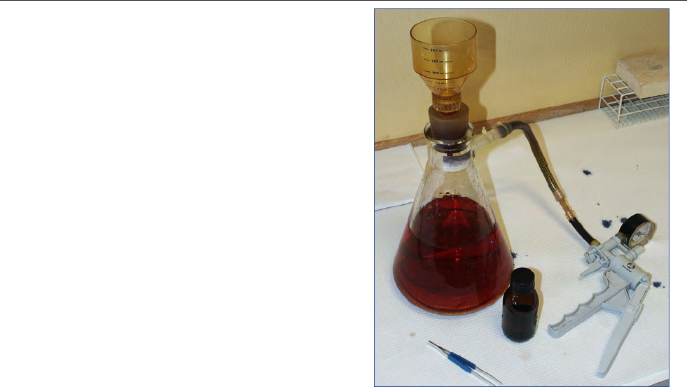
37
Microscopic and Molecular Methods for Quantitative Phytoplankton Analysis
Chapter 6 Filtering - semitransparent filters
Introduction
Phytoplankton species such as large dinoflagellates are often
present in the water column in low cell densities. Thus, samp-
les must first be concentrated in order to accurately quantify
these species. One method for concentrating phytoplankton
cells in water samples is the use of semitransparent membrane
filters (Fournier 1978). In this method water samples are di-
rectly filtered on a membrane filter which then is placed un-
der the microscope for the identification and enumeration of
phytoplankton cells.
Materials
Laboratory facilities
No specialised laboratory facilities are necessary for this met-
hod. Water samples using preservatives with potential harm-
ful effects should be handled following the appropriate health
and safety procedures.
Equipment
The following equipment is required:
• Compound light microscope, with at least 100X and
200X times magnification.
• Filter manifold and vacuum pump (handpump or elec-
tric) with manometer to gauge the pressure.
• Forceps for handling filters.
Chemicals and consumables
The following consumables are required:
• Semitransparent membrane filter (e.g. PALL GN-6). The
filters are availaible in a variety of diameters and pore si-
zes. A filter diameter of 25 mm and a pore size of 0.45
µm is recommended for use in this method.
• Glass microscope slides and coverslips.
• Lugol’s iodine solution is recommended.
• Glass bottles (dark) for sampling, transport and storage
of water samples.
Methods
The recommended preparation procedure is as follows:
1 The filtration manifold is assembled and the vacuum
pump tested (Fig. 1);
2 Using forceps, the filter is placed in the filter holder. The
funnel and holder are connected securely to prevent lea-
kage;
3 The preserved sample is gently agitated, by inverting the
sample bottle at least 10 times;
4 The volume to be filtered is measured using a graduated
cylinder. The most appropriate volume for analysis may
vary with location and time of year. Too many organisms
6 Filtering – semitransparent filters for for quantitative
phytoplankton analysis
Einar Dahl & Lars-Johan Naustvoll*
Institute of Marine Research, Flødevigen Marine Research Station, N-4817 HIS, Norway
*Author for correspondence e-mail: [email protected]
on the filter will prevent the identification of some spe-
cies. A guiding volume could be 25 mL for estuaries with
high production, 50 mL for inshore stations and 100 mL
for offshore stations;
5 The contents of the graduated cylinder are transferred
into the funnel above the filter;
6 A gentle vacuum is applied for filtration, less than 1/6
atmosphere (125 mm Hg), using a hand or electric pump
with manometer. A low vacuum pressure prevents de-
struction of and minimises distortion of fragile cells.
7 Filtering continues until the filter is “dry”;
8 The filter is removed from the filtration apparatus using
forceps and placed on a microscope slide;
9 The slide is analysed using a compound light microscope
at the desired magnification. The concentration of phy-
toplankton is calculated based on the number of cells
counted on the whole filter and the volume of sample
initially filtered.
To calculate the concentration (cells L
-1
) of the different spe-
cies in your preparation you must know:
V = Volume of sample concentrated on the filter (mL).
B
a
= Area of the filter (mm
2
).
B
c
= Area of the part of the filter counted (mm
2
).
N = Number of cells counted for the species of interest
Figure 1. Filtration manifold and hand held vacuum pump.

IOC Manuals & Guides no 55
Chapter 6 Filtering - semitransparent filters
38
Scope
Concentration and enumeration of phytoplankton, particularly
large and more physically robust species.
Detection range
10-50 cells per Litre, depending on volume filtered.
Advantages
This is a rapid and flexible method for the concentration of
phytoplankton using standard easy to use laboratory equip-
ment. The volume to be analysed can be easily adjusted depen-
ding on cell density.
Drawbacks
Fragile cells can be destroyed during the filtration process.
Type of training needed
No special training is required for the preparation of samples.
Taxonomic competence required for identification and enume-
ration.
Essential equipment
Compound light microscope, filtration manifold, vacuum
pump, forceps, semitransparent filters and microscope slides.
Equipment cost*
Microscope: Depending on manufacturer and type, from 4000
€ (6000 US $)
Filtration manifold: from 250 € (320 US $)
Vacuum pump: hand held from 180 € (240 US $)
The fundamentals of
The filtering - semitransparent filters method
Consumables, cost per sample**
Cost for filters and glass is approximately 1 € (1.5 US $).
Processing time per sample
Preparation time for the filters is 5 to 10 minutes, depending
volume filtered, amount of phytoplankton and filtration vo-
lume.
Analysis time per sample
Analysis time is about 30 minutes for target species, depending
on skill, quantity of phytoplankton cells and number of target
species.
Sample throughput per person per day
10-12 samples per day.
Health and Safety issues
Some fixatives that are used for phytoplankton preservation
could be potential harmful. Appropriate health and safety pro-
cedures must be followed at all times. Continual microscope
work could result in strain injury. It is important to incorporate
breaks into the daily analyses time. Ergonomic adjustments to
the microscope and the working place is recomended.
*service contracts not included
**salaries not included
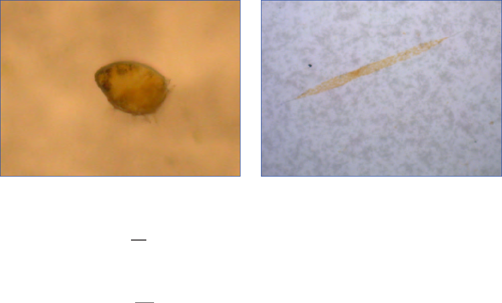
39
Microscopic and Molecular Methods for Quantitative Phytoplankton Analysis
Chapter 6 Filtering - semitransparent filters
The conversion factor (CF):
The concentration of the species C (cells mL
-1
) is then:
The conversion factors must be calculated for each filtering
unit and microscope as well as for each combination of sub-
sampling area and magnification.
Preservation and storage
Water samples can be preserved with neutralised formalde-
hyde or neutral Lugol’s iodine solution. Formaldehyde should
be used with care because of its toxicity and potential to trig-
ger allergic reactions. Neutral Lugol’s iodine solution is re-
commended for this method. If necessary, the brownish colo-
ration of the algae caused by this preservative can be removed
by oxidising the Lugol’s iodine using a few drops of sodium
thiosulfate per mL (3 g Na
2
S
2
O
3
in 100 mL water). When
using Lugol’s iodine solution the water samples should be sto-
red in dark glass bottles in the dark. Samples should retain the
colour of ‘weak tea’. The fixation of archived samples should
be checked every third month and additional Lugol’s iodine
should be added if the sample has lost its colouration. Pro-
perly fixed samples can last for years with appropriate main-
tenance.
Once a sample has been filtered it should be analysed im-
mediately. It is possible to store samples for one day, but this
may impede taxonomic identification. If samples are to be
stored the filter should be kept moist. A drop of filtered sea-
water should be added to the filter on the microscope slide.
A cover slip should be placed on top of the filter and gently
pressed downward. The microscope slide is then placed in the
refrigerator to reduce any evaporation. If the filter has dried
a new drop of seawater should be added without lifting the
cover slip prior to analysis of the sample on the microscope.
Discussion
Filtering with semitransparent filters is a rapid method for
concentrating phytoplankton samples before enumeration us-
ing light microscopy. It is a flexible method as the volume fil-
tered can be easily altered depending on the target species for
analysis. The detection limit can be improved by increasing
the volume filtered. The equipment needed for this concen-
tration method is standard laboratory equipment and rela-
tively inexpensive to purchase.
The main advantage of using the filtration method is the
short handling time from when the water sample arrives in
the laboratory to when it is analysed. The pore size of the
filters determines the size of the cells retained. If only a de-
fined size fraction of the phytoplankton is of interest, using
filters with a specific pore size could be advantageous as this
reduces the amount of background non target particles. The
equipment needed for the method is in most cases relatively
straightforward, compact and easy to use in the field.
The method has some disadvantages compared to other
methods. Some difficulties may arise in the taxonomic char-
acterisation of phytoplankton cells on filters as they cannot be
physically manipulated to change their orientation to allow
better examination of morphological features. Any non ran-
dom distribution on the filter could interfere with the results
if only a portion of the filter is analysed. The main disad-
vantage of this method is that cells can become distorted, or
destroyed during the filtration process. This method is not
recommended for fragile and delicate phytoplankton species,
e.g. Haptophytes and Chrysophytes, since these species would
be unidentifiable after the treatment. The semitransparent fil-
ter method favours the more robust species, e.g. diatoms and
thecate dinoflagellates (Figs. 2 and 3).
References
Fournier RO (1978) Membrane filtering. In: Sournia, A (ed)
Phytoplankton manual. Monographs on oceanographic method-
ology 6, Unesco, Paris, p. 108-112
Figure 2. Dinophysis sp. observed on a semitransparent filter.
Figure 3. Rhizosolenia sp. observed on a semitransparent filter.
V
CF
NC *=
c
a
B
B
CF =
IOC Manuals & Guides no 55
40
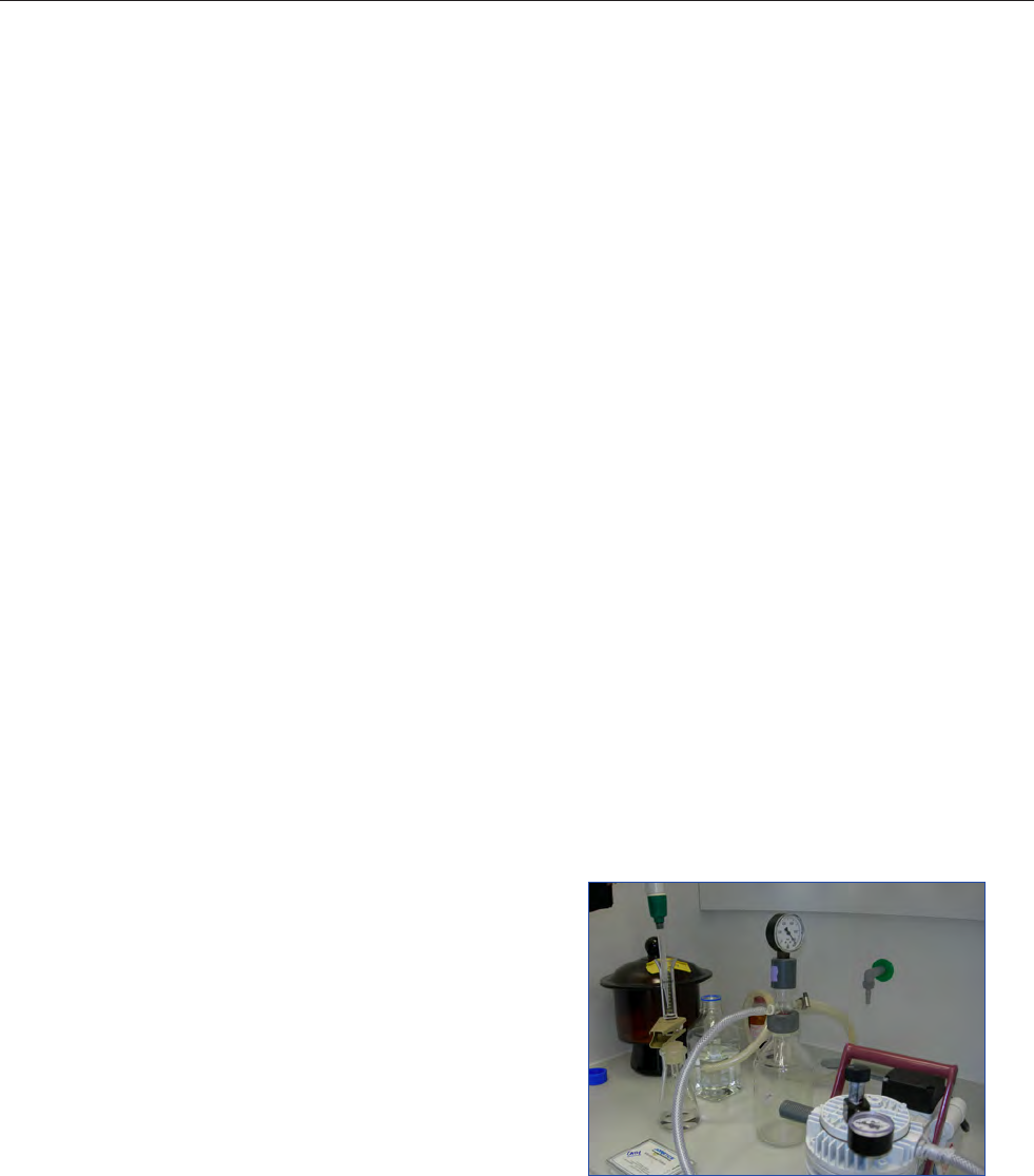
41
Microscopic and Molecular Methods for Quantitative Phytoplankton Analysis
Chapter 7 Filter - transfer - freeze
Introduction
Precise and accurate identification and enumeration of phy-
toplankton cells in field samples is fundamental to the main-
tenance of time-series data on distribution and abundance
of taxa, as well as for biological oceanographic research and
plankton surveillance programmes, e.g. for harmful algal
blooms. Such counting methods are also required for cell enu-
meration in unialgal or multialgal cultures for laboratory or
mesocosm experiments on phytoplankton. In this sense, the
term “phytoplankton” is used loosely to include all eukaryo-
tic microalgae, protists, cyanobacteria and unicellular benthic
and epiphytic taxa, including cysts and other resting stages.
Both “classical” methods based upon microscopic observa-
tions of morphological features of whole cells and molecular
methods (nucleic acid hybridisation, antibodies, lectins, etc.)
are now available for comparison (Godhe et al. 2007).
Although the filter-transfer-freeze (FTF) technique is consi-
dered among the classical approaches for cell counting and
identification, it is not specifically a cell enumeration met-
hod, but rather a means of cell concentration, collection,
and transfer for counting by alternative means. When app-
lied correctly, the accuracy and reproducibility of cell counts
performed by the FTF technique is more a function of the
subsequent counting and identification methods than of the
FTF procedure itself. The FTF method was introduced more
than two decades ago (Hewes and Holm-Hansen 1983), but
in spite of its simplicity and proven effectiveness, the method
has not been widely employed. This is regrettable because the
FTF method can be applied for both critical taxonomy (with
some caveats) and for rapid but superficial analysis of phy-
toplankton samples. The original method was designed with
respect to nanoplankton and indeed appears to work best for
taxa in the size range of ca. 5 – 200 µm diameter. Smaller cells
tend to get lost to the filter and larger organisms do not trans-
fer well. Nevertheless, this size-range embraces most of the
diatoms and nanoflagellates of interest and chain-formation
does not markedly decrease transfer efficiency from the filter
to slide. The method has been rigorously tested for use in
field monitoring of phytoplankton in the Gulf of St. Lawren-
ce region of Atlantic Canada (J. Smith and K. Pauley, Dept.
of Fisheries and Oceans, Canada, unpublished manual) and
in comparison with alternative methods for counting cells in
cultures of the marine dinoflagellate genus Alexandrium (Ra-
fuse 2004). Consolidation of the methodological variants in
this chapter may assist in wider dissemination of this rather
neglected method for phytoplankton cell enumeration.
Materials
Equipment
• Electric or manual vacuum pump (preferably with va-
cuum gauge)
• Filtration apparatus (funnel, clamp, frit, rubber stopper,
connecting rubber or Tygon tubing) – single or multiple
as required
• Vacuum trap flask (if connected to electric pump)
• Waste disposal flask (for filtered fixatives/preservatives)
• Freezer (-20 ˚C), dry ice or cold block (prefrozen)
• Digital or mechanical cell counter (optional)
• Research microscope equipped with bright-field, phase-
contrast or Normarski optics
• Standard glass microscope slides
• Glass cover slips (24 x 24 or 24 x 50 mm)
• Watch glass
• Polycarbonate membrane filters (25 mm); Poretics™ or
Nuclepore™ (pore size: 3 µm or dependent upon size
distribution of taxa of interest)
• Pasteur pipettes with rubber bulb
• 0.5 or 1.0 l plastic squirt bottle
• Millipore-type flat forceps
• Grease pencil (optional)
• Source of filtered (0.22 µm) seawater
• Fixatives/preservatives (if desired)
• 95% or 70% ethanol (for cleaning)
Laboratory facilities
The FTF method and subsequent microscopic analysis requi-
re no sophisticated facilities. The technique can be performed
even in a rudimentary “laboratory”, at dockside or on board
ship, if a means of quick freezing of the slide is available. In
the absence of a laboratory freezer, the slide can be frozen
upon dry ice, liquid nitrogen (carefully!) or upon an alumi-
num or plastic cold block that has been prefrozen at -20 to
-80 ˚C and maintained in a well-insulated container. The ba-
7 The filter - transfer - freeze method for quantitative
phytoplankton analysis
Allan Cembella*
1
and Cheryl Rafuse
2
1
Alfred Wegener Institute for Polar and Marine Research, Am Handelshafen 12, D-27570 Bremerhaven, Germany
2
Institute for Marine Biosciences, National Research Council of Canada, 1411 Oxford Street, Halifax, Canada
*Author for correspondence: [email protected]
Figure 1. Filtration and vacuum apparatus used in the FTF method.

IOC Manuals & Guides no 55
Chapter 7 Filter - transfer - freeze
42
Scope
Appropriate for fixed, labelled, or unfixed planktonic chain-for-
ming or unicellular organisms.
Detection range
Detection range is dependent on the volume filtered. Best pre-
cision and counting accuracy is achieved with transfer of 200
– 400 cells per taxon of interest to the slide surface.
Advantages
Can be applied for enumeration of cells prepared with a variety
of different preservation and labelling methods or from fresh
samples. The method can accommodate alternative microsco-
pic techniques: bright field, phase-contrast, Normarski, and
epifluorescence methods. The preparation is extremely simple
and rapid (minutes) and is limited only by the filtration time.
Drawbacks
Potential loss of cells in the transfer process and some morpho-
logical distortion of delicate specimens is possible. The filtration
and microscopic method is normally applied serially, i.e. one
sample at a time, although in principle multiple filtration fun-
nels could be used to filter samples in parallel. Other limitations
of the method are generic to all optical microscopic techniques
(resolution limit, operator error in identification, etc.).
Type of training needed
Only a simple practical demonstration of the filtration and
transfer method is required – this method can be mastered in
<1 hour with an expected unsuccessful transfer occurring only
in the first five attempts. Phytoplankton identification requi-
res continuous training over years with in-depth knowledge of
taxonomic literature.
Essential Equipment
Vacuum filtration apparatus with pump, optical microscope
and a source of rapid freezing (-20 ºC freezer, dry ice, or cold
block).
Equipment cost*
100 – 2000 € (excluding microscope). Estimated cost for accep-
table microscope ranges from 3,000 € for a simple bright field
or student-grade microscope to >60,000 € for a fully equipped
research microscope with Normarski or epifluorence capabili-
ties.
Consumables, cost per sample**
Less than 2 €/2 US $ (determined mostly by the cost of the
filter).
Processing time per sample before analysis
Varies with the volume of water filtered, but typically <5 mi-
nutes.
Analysis time per sample
Limited by the degree of scrutiny required and the complexity
of the sample. For accurate and precise counts from monocultu-
res or simple mixtures <10 minutes would be expected, whereas
for complex plankton matrices from dense field samples up to 1
hour per sample may be required. These timings are dependent
on the skill of the analyst.
Sample throughput per person per day
10 – 50 samples per day (8 working hours), depending upon
the cell concentration and sample complexity.
No. of samples processed in parallel
Up to 12 filtrations may be carried out simultaneously, but mi-
croscopic observations must be in series.
Health and Safety issues
Determined only by the toxicity of the fixative and labelling
components (if any) used for the preparation of the samples.
Appropriate health and safety procedures must be followed at
all times. Continual microscope work could result in strain
injury. It is important to incorporate breaks into the daily ana-
lyses time. Ergonomic adjustments to the microscope and the
working place is recomended.
*service contracts not included
**salaries not included
The fundamentals of
The filter - transfer - freeze method
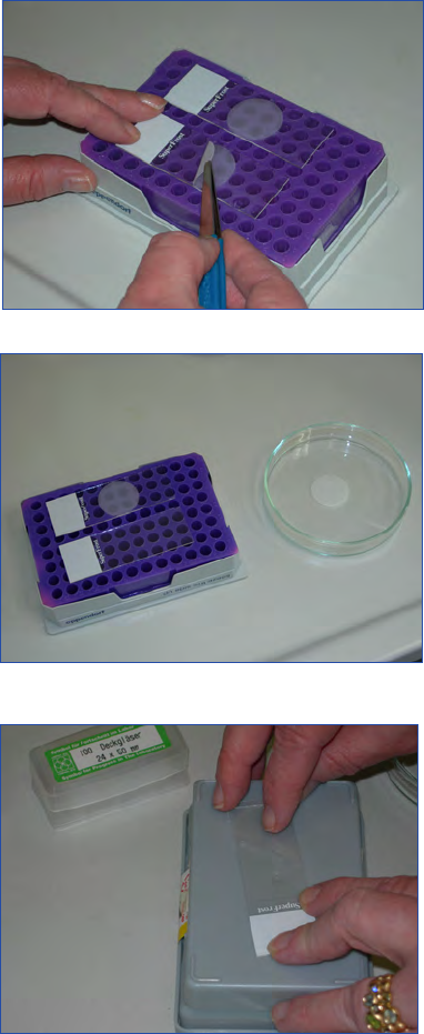
43
Microscopic and Molecular Methods for Quantitative Phytoplankton Analysis
Chapter 7 Filter - transfer - freeze
sic requirements are approximately 1 m
2
free bench space for
vacuum pump, filtration apparatus, in addition to space for
mounting of a standard microscope.
Methods
Sample collection, fixation, storage and preparation for mi-
croscopic analysis have been well described in the UNESCO
Manual on Harmful Marine Microalgae in the chapter by
Andersen and Throndsen (2004) on estimating cell numbers.
This reference should be consulted for general procedures.
Only specifics relevant to the FTF method are provided here
as follows:
1 Prepare a clean glass microscope slide by outlining a
circular filter-separator (25 mm) with a black grease pencil.
This step may be omitted as it does not always provide an
advantage for corralling the cells on the slide;
2 Mount a polycarbonate membrane filter (25 mm diame-
ter) onto the the filtration apparatus and ensure that the
filter remains centred when clamping or threading the fil-
tration funnel (Fig. 1);
3 Filter a suitable volume of plankton sample (must be deter-
mined empirically after initial trials and rough counting of
taxa of interest) under gentle vacuum (<200 mm Hg) but
at a suitable flow rate (ca. 50 mL min
-1
);
4 Continue filtration until a few drops are left in the fun-
nel, then turn off pump and allow the residual vacuum to
draw the filter just to the point of dryness. Release vacuum
slowly;
5 Remove the filtration funnel and with flat forceps (Mil-
lipore™- type) carefully lift off the filter, invert it onto the
centre of the prepared glass slide (in the centre of the grease
pencil ring if this step was followed);
6 Place the glass slide onto a cold flat surface (dry ice or cold
block in the freezer) filter side up and allow the filter to
freeze completely to the slide (usually two minutes is suf-
ficient time);
7 Remove the glass slide from the cold surface or from the
freezer, and place on a flat counter area with the filter side up;
8 If the filter slide is crackling frozen, wait a few seconds
until the frost just begins to disappear. With a flat forceps,
grasp the edge of the filter and with a smooth rolling mo-
tion of the hand, peel back the filter parallel to the speci-
men surface until the filter is free from the slide. A deposit
of material should be apparent at the centre of the slide
(Fig. 2). Retain the filter (shiny side up) in a watch glass or
Petri dish for further observation (Fig. 3);
9 Add a drop or two of filtered seawater (0.22 µm) with a
Pasteur pipette to the sample at the centre of slide. Place
the glass coverslip (25 x 50 mm) carefully upon the glass
slide (Fig. 4);
10 Identify and count the cells by viewing the entire contents
trapped inside the grease chalk circle or under the entire
cover slip. Cells should be counted in zigzag transects un-
der the appropriate magnification for identification;
11 Calculate cell numbers as the total cells counted on the
slide per unit volume of sample filtered (assumes 100%
transfer efficiency from the filter to the slide).
Useful notes on the application of the method
1 The optimal filter pore size must be determined by the
cell size of the taxa of interest, the concentration of the
suspended particulates in the seawater sample and the vo-
lume of seawater to be filtered. In general, use the largest
available pore size for the filter (to maximise flow through
and minimise clogging) that will retain all of the key taxa.
For nanoplankton samples, 3 or 5 µm pore size is usually a
good compromise;
Figure 2. Removal of filter from microscope slide using forceps.
Figure 3. Microscope slide after the filter has been removed. The
filter is retained in the Petri dish
Figure 4. A drop of seawater is added to the microscope slide
containing the sample and a coverslip added.
IOC Manuals & Guides no 55
Chapter 7 Filter - transfer - freeze
44
2 A drop or two of filtered seawater can be useful in seating
the filter on the filter apparatus. Make sure the filter is al-
ways mounted in the same orientation, usually shiny-side
up for most types (but check!);
3 It is not usually feasible to count more than a few hundred
cells of a given taxon on a single slide, but counts must be
sufficiently high (see Andersen and Throndsen 2004) to
avoid having to count many replicate slides for statistical
validity. The sample must be thoroughly homogenised in
the bottle by a gentle end-to-end and side-to-side rolling
motion between the hands before filtration;
4 A wet filter will result in the loss or mobilisation of cells on
the filter as it is removed from the funnel. This is likely to
be the largest source of error in the method. On the other
hand, sucking the filter under high vacuum to complete
dryness or for a prolonged time will embed the cells in the
membrane and they will not transfer efficiently from the
filter;
5 Make sure that there are no pleats or folds in the filter and
that the entire surface is in good contact with the slide;
6 Perform a cursory examination of the upper filter surface
for residual cells that were not transferred. This can be
done quickly with a stereo-microscope or a standard mi-
croscope under low power (40X). If more than a few cells
are present, the filtration procedure must be repeated;
7 This procedure is designed for immediate observation of
specimens without archiving. Techniques for preparing
semi-permanent mounting and embedding with various
preparations of glycerol and embedding medium for later
taxonomic analysis may be consulted in Hewes and Holm-
Hansen (1983);
8 Either of two techniques can be used for placing the cover
slip: 1) gently lowering one end of the coverslip until con-
tact is made with the water droplet, then letting surface
tension act as the cover slip is lowered at an angle; or 2) the
“bombardier principle”, whereby the cover slip is dropped
gently from just above the water droplet. Take care to avoid
bubbles under the coverslip.
Preservation and storage
The FTF method can be applied to microscopic analysis of
plankton samples directly from seawater, since filtration first
immobilises and quick-freezing kills the cells. Cells frozen to
the filter may be stored in the freezer for several hours (or even
overnight) without apparent damage or effect on subsequent
transfer. Nevertheless, for archival purposes, fixation and/or
preservation of cells may be desired to reduce decomposition
and to maintain morphology for future identification and
enumeration. Aldehyde preservatives affect steric configura-
tion by cross-linking of proteins via multiple interaction with
various amino acid residues and even peptide bonds (Shi et al.
2000), whereas ethanol is a coagulant fixative causing limited
and unstable cross-linkages. Although exhaustive comparative
trials have not been conducted specifically for the FTF meth-
od, all commonly used preservatives and fixatives (Keller and
Manak 1993, Amann 1995, Cañete et al. 2001), including
Lugol’s iodine solution, formulation of gluteraldehyde, for-
malin or paraformaldehyde (PFA) in various buffer solutions,
as well as saline-ethanol mixtures for application of molecular
probes are generally compatible with this method.
Details of fixation and preservation are beyond the scope of
this chapter, but a few general observations here with respect
to the FTF method are relevant. Lugol’s iodine solution has
been traditionally used to preserve microalgae for counts via
Utermöhl settling chamber method (see Chapter 2, this vol-
ume) and as such can be employed also for the FTF tech-
nique. The disadvantages of this solution are that it strongly
colours cells so that autotrophic and heterotrophic cells can-
not easily be distinguished and cells cannot be readily stained
for epifluorescence microscopy. Decolourisation (i.e. with
thiosulphate) is possible but often results in a loss of mor-
phological details and even cell lysis. Lugol’s solution is par-
ticularly effective with highly silicified structures, e.g. most
diatoms and silicoflagellates, but less so for naked and thecate
flagellates for which details are often obscured.
Gluteraldehyde is excellent for fixation and preservation of
structures, particularly for subsequent analysis by SEM or
TEM, but is relatively expensive and highly toxic. Use of
gluteraldehyde is therefore discouraged for the FTF method,
which does not usually yield the highest quality samples for
electron microscopy in any case. Other aldehydes fixatives are
preferred, for a compromise preservation of siliceous, calcare-
ous and cellulosic structures of phytoplankton. Acidic forma-
lin preparations can be very destructive to calcareous struc-
tures, such as those of coccolithophorids.
A high quality universal preservative for most phytoplankton
samples based upon buffered paraformaldehyde (PFA) has
been extensively tested with the FTF method. This formula-
tion stabilises most cell structures and provide a robust re-
sistance to filtration and freeze-thaw damage. The recipe is
therefore given here as follows:
Preparation of 10% PFA:
1 Add 100 g of PFA powder to 800 mL dH
2
O (or a suitable
buffer);
2 Heat to about 60-80
º
C with constant magnetic stirring;
3 Add NaOH (1N) gradually until PFA is just completely
dissolved (do not add too much!);
4 Let the solution cool to room temperature
5 Adjust to desired pH using NaOH or HCl (1N);
6 Add H
2
O (or buffer) to make up to 1000 mL.
For most plankton samples, acidity should be adjusted to pH
4 and final concentration in the sample should be 1 – 2%.
Thereafter, samples can be archived for many months prior to
filtration for FTF microscopic analysis.
Discussion
The FTF technique has some of the advantages and draw-
backs of other filtration-based techniques. Nevertheless, the
problems cited for direct counting of cells upon filters (morp-
hological distortion of cells, poor contrast, low resolution,
difficulty in applying stains, etc.) (Hewes and Holm-Hansen
1983) are effectively eliminated in the FTF method. Rela-
tive to other classical counting methods, such as the Uter-
45
Microscopic and Molecular Methods for Quantitative Phytoplankton Analysis
Chapter 7 Filter - transfer - freeze
möhl settling chamber method, the FTF technique has the
advantage that there is no time-lag for sedimentation, with
attendant concerns about physical disturbance of the setting
regime (e.g., on board ship). Counts can be performed with a
standard research microscope rather than with a less common
inverted optical system. As a cell concentration and transfer
technique, the FTF method can be successfully combined
with other methods for critical taxonomy by epifluorescence
microscopy, such as the calcofluor staining method for the
cellulose plates of dinoflagellates, or application of fluorescen-
ce probes for nucleic acids or antibody targets. In the fluores-
cence approach, the appropriate stains can be applied at the
edge of the cover slip and drawn across the sample by apply-
ing a laboratory tissue at the opposite corner of the cover slip.
Furthermore, FTF preparation time is only a few minutes,
with filtration as the rate-limiting step. This makes it easy to
adjust the cell concentration on the counting slide for opti-
mal accuracy and precision of counting (typically 200 - 400
cells per taxon of interest) by varying the volume filtration or
by diluting the sample with filtered seawater. The latter may
be important to avoid cell overlap, e.g. of diatom chains, or
clumping of aggregated cells, particularly of concentrated net
plankton hauls.
As with other filtration-based techniques, the physical loss
or damage of cells must be carefully monitored during the
preparation procedures. Sloppy filtration techniques, leakage
of the filtration funnels, overloading the filter and failure to
thoroughly clean the filtration apparatus with detergent bet-
ween usages, followed by rinsing with ethanol then deionised
water between each sample, can cause cell loss. Sometimes the
sample may leak outside of the grease chalk circle and there-
fore may not be counted; for this reason it is often preferable
to eliminate this circle and merely count the entire surface
area under the cover slip.
In comparative testing of the FTF method against whole-cell
fluorescence in situ hybridization (FISH) and the Utermöhl
settling chamber methods for counting cultured cells of the
marine dinoflagellates Alexandrium tamarense and A. osten-
feldii (Rafuse 2004), the filtration-based methods yielded a
consistently higher coefficient of variation, most of which was
attributed to variable cell loss. Yet in a detailed comparison of
17 alternative cell counting methods for A. fundyense (Godhe
at al. 2007), the FTF method exhibited among the lowest
standard errors among replicate counts (n = 4 or 5) within the
concentration range of 102 to 105 cells L
-1
. During the filtra-
tion step, cells can be lost within the filtration apparatus, i.e.
between the funnel and base or via leakage from the interface
between the filter holder and the filter. All standard funnel fil-
tration apparatus (Fig. 1), such as the common clamp-systems
obtainable from Millipore™, Gelman/Pall™, Sartorius™,
etc., are acceptable for this method, including the threaded
mounting (Radnoti™-type) systems for attaching the funnel
to the filter base. The clamp-type systems are preferable be-
cause they are simpler and do not permit the possible loss of
cells between the O-rings (Rafuse 2004) that may occur for
threaded-type filter systems. Evidence of this cell loss from
concentrated samples may be observed by visual inspection
of the funnels and other components after the filter is remo-
ved. Use of glass versus plastic (polystyrene) funnels does not
appear to be critical, but the funnels should be transparent
to observe the filtration process. To maximize transfer of all
cells to the filter, the filtration should proceed until the filter
surface is just dry (i.e. the upper surface is no longer shiny),
but not beyond this point, to preserve cell integrity. Dirty ap-
paratus and ultra-slow filtration (<2 mL min
-1
) can also lead
to adherence of cells to the walls of the filtration funnel; such
loss can be considerable – >5% of cells under a worst case sce-
nario and often taxonomically biased towards mucilaginous
cells or aggregates. In any case, this selective loss from the
harvested sample can be verified if necessary by thoroughly
washing down the walls of the funnel system with a high-
pressure stream of filtered seawater from a squirt bottle and
recovering the cells on a fresh filter under gentle vacuum. If
few cells are found, loss of cells in the system can be assumed
to be minimal.
Breakage of cells upon contact with the filter surface, and es-
pecially sucking the filter beyond the dry point under high va-
cuum can also account for considerable cell loss or distortion
in all filter-based methods. For this reason, vacuum pressure
should be kept low (<15 mm Hg) but substantial enough to
ensure a steady flow of filtrate (a couple of drops per second
or about 50 mL min
-1
is acceptable). Correct operation of the
filtration protocol can be verified by observation under a dis-
secting microscope of random or haphazard distribution cells
on the upper filter surface of unialgal cultures. For mixed algal
assemblages, evidence of clumping or patchy cell distribution
over the filter surface is a sign of poor filtration technique.
The foregoing are generic strengths and weaknesses of all fil-
tration-based counting methods. Surprisingly, two elements
that are specific to the FTF method – freeze-thaw and filter-
transfer – do not contribute in a major way to cell loss or
morphological distortions when the method is applied cor-
rectly. Quick freezing is preferable to slower methods since
the former leads to less crystal formation and hence less cell
breakage. Cells may also break when the filter is ripped off the
frozen sample that contains the cells, or if the cells are weak,
not completely frozen, or have thawed too quickly. Practice
will generally ensure excellent reproducibility.
Acknowledgements
The authors are indebted to J.C. Smith and K. Pauley, Gulf
Fisheries Centre, Dept. of Fisheries and Oceans, Canada for
collating details of the method in the unpublished field and
laboratory manual for the collection, identification and enu-
meration of toxic marine phytoplankton from southern and
eastern regions of the Gulf of St. Lawrence.
References
Amann R (1995) In situ identification of micro-organisms by whole
cell hybridization with rRNA-targeted nucleic acid probes. Mol
Microb Ecol Manual 3.3.6: 1-15
Andersen P, Throndsen J (2004) Estimating cell numbers. In: Halle-
graeff GM, Anderson DM, Cembella AD (eds) Manual on harm-
ful marine microalgae, Monographs on oceanographic methodo-
logy. UNESCO Publishing, Paris, 99-129
Cañete M, Juarranz A, López-Nieva P, Alonso-Torcal C, Villanueva
A, Stockert C (2001) Fixation and permanent mounting of fluo-
rescent probes after vital labelling of cultured cells. Acta Histo-
IOC Manuals & Guides no 55
Chapter 7 Filter - transfer - freeze
46
chem 103: 117-126
Godhe A, Cusack C, Pedersen J, Andersen P, Anderson DM, Bres-
nan E, Cembella A, Dahl E, Diercks S, Elbrächter M, Edler L,
Galuzzi L, Gescher C, Gladstone M, Karlson B, Kulis D, LeGres-
ley M, Lindahl O, Marin R, McDermott G, Medlin MK, Naust-
voll L-J, Penna A, Töbe K (2007) Intercalibration of classical and
molecular techniques for identification of Alexandrium fundyense
(Dinophyceae) and estimation of cell densities. Harmful Algae 6:
56-72
Hewes D, Holm-Hansen, O (1983) A method for recovering na-
noplankton from filters for identification with the microscope:
the filter-transfer-freeze (FTF) technique. Limnol Oceanogr 28:
389–394
Keller GH, Manak MM (1993) DNA probes. Second Edition,
Stockton Press, New York, USA
Rafuse C (2004) Effects of physiological and environmental condi-
tions on rRNA probes for two species of microalgae, Alexandrium
ostenfeldii and A. tamarense. MS dissertation, Dalhousie Univer-
sity, Halifax, Canada
Shi S-R, Gu J, Taylor CR (eds) (2000) Antigen retrieval techniques:
immunohistochemistry and molecular morphology. Eaton Pub-
lishing, Natick, MA, USA
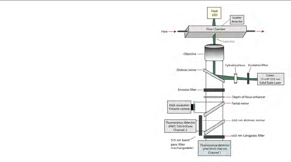
47
Microscopic and Molecular Methods for Quantitative Phytoplankton Analysis
Chapter 8 Imaging flow cytometry - FlowCAM
Introduction
In water quality analysis and monitoring the ability to count,
capture and save images of the particles or organisms in a sam-
ple is advantageous. Traditional “particle counting” methods,
such as microscope particle analysis, can be slow and tedious.
The FlowCAM, an imaging flow cytometer developed by
Fluid Imaging Technologies, captures digital images of par-
ticles in a fluid stream using laser light detection, enabling the
measurement of many cell parameters, such as length, width,
equivalent spherical diameter and fluorescence (Sieracki et al.
1998). The captured images from a sample can be studied vi-
sually as well as post-processed by a computer to automatical-
ly search for particles of a certain type or class. The FlowCAM
detects and measures fluorescence emissions at two different
wavelengths, typically red and orange fluorescence, indicating
the presence of chlorophyll or phycoerythrin within the indi-
vidual particles/cells in a field sample. This technology is very
similar to a flow cytometer that captures only fluorescence
and scatter properties of a particle. However, the FlowCAM
merges the technologies of a flow cytometer and an imaging
microscope – resulting in the Flow Cytometer and Microsco-
pe (FlowCAM – Fig. 1). The FlowCAM automatically counts
and images particles or cells in a discrete sample. Using the
image analysis data generated during sample processing, the
FlowCAM software uses image libraries previously created by
the user of target groups or classes that can assist in analysis
and classification. Overall, the FlowCAM can be customised
to accommodate most field environments and can be used
to detect and quantify different algal groups within a sample
(Zarauz et al. 2009), including harmful algal species (Buskey
and Hyatt 2006).
Materials
Equipment
For quantitative microphytoplankton analysis (20-300 µm)
a Benchtop or Portable FlowCAM (VS IV) is required (Figs
2 & 3). The FlowCAM must be equipped with either a blue
(488 nm) or green laser (532 nm) for fluorescent and par-
ticle detection. In addition the instrument should have and
be setup with, a 4X or 10X objective depending on the size of
the cells to be visualised and quantified. Each objective must
use a corresponding rectangular. tubular glass Flow Cell (100
or 300 µm depth) in which all cells are to be analysed. For dis-
crete volume sampling a funnel stand or pipet tip apparatus
must be used, as provided with the instrument.
Chemicals and consumables
• Filtered Seawater (FSW)
• Distilled water
• Calibration Beads (5, 10, 20, 50 & 100 µm)
• Disposable plastic pipets tips (1-10 mLs)
• Small funnels
• FlowCAM Flow Cells (100 or 300 µm depth)
• Silicone Tubing
• Nylon mesh (100 or 300 µm)
• Graduated cylinders to measure volumes to be processed
Solutions for preservation
• 10% buffered formalin solution (see Appendix 1 for pre-
paration instructions)
• Formalin: Acetic acid (see Appendix 1)
Methods
The FlowCAM was originally developed for phytoplankton
detection and quantification and is ideally suited for analysis
of natural field samples that contain specific groups or species
of microplankton that are usually counted using traditional
microscopic techniques. To begin, the FlowCAM (including
the integrated computer) and laser need to be turned on, and
the laser allowed to warm up for approximately 20 minutes
(according to FlowCAM manual). FlowCAMs are equipped
with either a green or blue laser; both can be used for algal
fluorescence detection. As the FlowCAM laser is warming
8 Imaging flow cytometry for quantitative
phytoplankton analysis — FlowCAM
Nicole J. Poulton*
1
and Jennifer L. Martin
2
1
J.J. MacIsaac Aquatic Cytometry, Facility Bigelow Laboratory for Ocean Sciences, 180 McKown Point Road, P.O. Box 475 West Boothbay
Harbor, ME 04575, USA
2
Fisheries and Oceans Canada Biological Station, 531 Brandy Cove Road, St. Andrews, NB E5B 2L9, Canada
*Author for correspondence: npoulton@bigelow.org
Figure 1. Illustration of the fluidics and optics of the FlowCAM.

IOC Manuals & Guides no 55
Chapter 8 Imaging flow cytometry - FlowCAM
48
Scope
The FlowCAM method captures digital images of particles and/
or cells. This enables the instrument to measure cell abundance
and many cell parameters, such as length, width, equivalent
spherical diameter and fluorescence.
Detection range
The detection range depends on the volume of sample analy-
sed.
Advantages
Manual labour required for processing and handling is mini-
mised, compared to traditional microscopy techniques. The
method produces a non-biased digital record and instantaneous
image analysis data on every particle or cell within a sample.
The captured images from a sample can be studied visually as
well as post-processed by a computer to search and quantify
cells of a certain type or class. Portable FlowCAMs are also av-
ailable for field measurements.
Drawbacks
Cells are required to have a distinct morphology to be readily
identified by FlowCAM. Different objectives are needed for
different phytoplankton size ranges. Preservation of the sam-
ple is not recommended, live samples are optimal, as cell auto-
fluorescence can decline or is removed with certain preservation
techniques (ie. Utermohls). Heavy particle loads (riverine or
estuaries) could interfere with image capture – dilution of the
sample for accurate abundances may be required.
Type of training needed
1. To use FlowCAM: Approximately one-two days of training
would be required with guidance from a trained individual and
follow-up support.
2. To troubleshoot and QC: A more experienced analyst with
up to 6 months experience would be more effective at troubles-
hooting the instrument. The company that manufactures the
FlowCAM, Fluid Imaging Technologies, provides on-site, web-
based, and over the phone customer assistance when needed.
3. Taxonomic expertise is required to interpret images and re-
sults.
Essential Equipment
FlowCAM VS IV with 4X & 10X objectives, associated Visu-
alSpreadsheet (ViSp) software, and Flow Cells.
Equipment cost*
$75,000-85,000 US (depends on the model – Benchtop or Por-
table), see Appendix 2.
Consumables, cost per sample**
1-5 US dollars.
Processing time per sample before analysis
Ranges from 15 minutes-1 hour depending on the volume run
and particle density.
Analysis time per sample
Ranges from 1 hour to minutes. The time consuming part is
identifying cells and developing image libraries for automated
sample analysis (hours of time upfront).
Sample throughput per person per day
4-36 depending on the time of run and analysis time.
No. of samples processed in parallel
One sample at at time.
Health and Safety issues
Minimal, caution and general safety practices must be used
when using the laser within the instrument and preserved sam-
ples.
*service contracts not included
**salaries not included
The fundamentals of
The FlowCAM - maging flow cytometer method
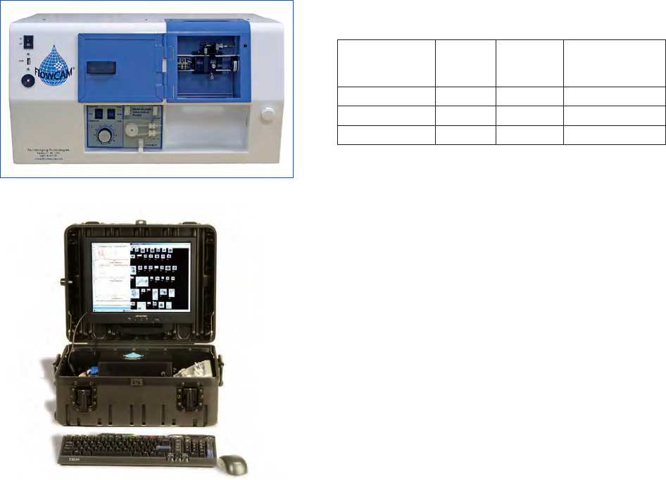
49
Microscopic and Molecular Methods for Quantitative Phytoplankton Analysis
Chapter 8 Imaging flow cytometry - FlowCAM
up, the FlowCAM VisualSpreadsheet (ViSp) software can be
started.
Before running natural field samples, the FlowCAM needs to
be ”setup”, meaning the values for triggering using fluores-
cent detection (thresholds) and the cell size range of particles
to be collected need to be determined. The FlowCAM also
needs to be properly focused, similar to how a microscope
would work. In order to get good visualisation of the particles
in each sample optimal focus is required. The set up process
usually takes between 20-40 minutes. Once the settings for
microplankton detection are determined the settings do not
change between samples, unless the ecosystem or background
within a sample (such as particle load) changes. More details
on how to set up the instrument can be found in the Flow-
CAM Operators Manual (Anonymous 2009).
For analysing and counting microplankton in natural field
samples 4X, 10X or 20X objective are usually used in com-
bination with an appropriate Flow Cell (Table 1). The Flow
Cell is a rectangular glass tube that can vary in size depen-
ding on the objective used. Silicone tubing is affixed to both
ends and allows the sample to pass through the tube to a pe-
ristaltic pump downstream of the Flow Cell. The Flow Cell
mimics the glass side of a microscope. Note that the Flow
Cell is oriented vertically in the instrument differing from the
microscope mounted slide that is positioned horizontally. In-
stallation of a 100 µm depth Flow Cell is described in Fig. 4.
Data Acquisition
1 Each field sample needs to be thoroughly mixed by gentle
rotation to resuspend any particles that may have settled;
2 Using a graduated cylinder, a predetermined volume of
each sample is dispensed into a funnel or pipet tip;
3 Set the ViSp FlowCAM software to start analysis and col-
lect the data (file folder name and location) in Trigger
mode;
4 Start the peristaltic pump, once data acquisition in the
ViSp FlowCAM software begins the sample will now be
analysed for fluorescent events (phytoplankton) that pass
by the laser that is aligned with the Flow Cell.
For most field samples, between 10-100 mL of each sample
is analysed and processed. Sample processing rate (flow rate)
will depend on the density of cells in the field sample, and
the dimensions of the Flow Cell used. As a starting point, set
the standard VWR pump to fast mode and the speed dial to
5. As the sample is flowing through the Flow Cell, check the
fluorescence trigger rate using ”Trigger Mode Setup”. If the
images are appearing at a rate more than one per second begin
to turn down the flowrate of the pump until the optimum
level is attained. In somes cases the microphytoplankton con-
centration will be low and there will appear to be no trigger
events. The user should be aware that increasing the flowrate
too much (PRIME mode) may cause image distortion and
prevent accurate image capture. To test the fluorescence set-
tings (thresholds) of the FlowCAM it is recommended that a
diluted phytoplankton culture (100-1000 fold) be used ini-
tially to verify the settings being used. It is essential that the
Flow Cell and funnel are rinsed throughly afterwards to pre-
vent contamination of subsequent samples to be quantified
and analysed. Typically, a field sample can be processed in
30-40 minutes.
During the run, the operator should occasionally mix the
sample in the funnel using a pipette to prevent particles or
cells from settling. The operator should also check the Flow
Cell for any potential clogs or blockages. If clogging occurs,
the user would typically observe particles sitting at the en-
trance to the glass tubing. If a clog occurs the operator should
end the run and restart the analysis. To prevent clogging from
occurring, screening or sieving the sample prior to analysis
is recommended using nylon mesh (100 or 300 µm) depen-
ding on the depth of the Flow Cell being used. During a run
the operator should also periodically pinch the tubing down
stream of the Flow Cell in order to prevent large particles
from blocking the entrance to the Flow Cell. Near the end
of a run the funnel should be rinsed with FSW to ensure all
particles are removed from the funnel (and have entered the
Figure 2. Benchtop FlowCAM.
Figure 3. Portable FlowCAM (VS IV).
Cell Size Range Objective Flow Cell Flow Cell
Dimensions
(Depth x Width)
10 µm – 100 µm 10 X FC100 100 µm x 2 mm
20 µm – 300 µm 4 X FC300 300 µm x 3 mm
60 µm – 600 µm 4 X FC600 600 µm x 6 mm
Table 1. Recommended cell size range (diameter) and objectives
for different FlowCAM Flow Cells.
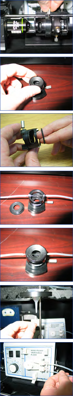
IOC Manuals & Guides no 55
Chapter 8 Imaging flow cytometry - FlowCAM
50
Step 1. Remove the CH300 Flow Cell Holder from the Focu-
sing Collar by loosening the thumb screw and pulling the Flow
Cell Holder away from the focusing rails. Loosening the thumb
screw is accomplished by turning the screw counter-clockwise.
The 10X objective can be replaced with a 4X objective.
Step 2. Unscrew the retaining cap from the Flow Cell Holder.
This is accomplished by turning the cap counterclockwise until
it separates from the Flow Cell Holder.
Step 3. For some FlowCAM models the CH300 Flow Cell Hol-
der has a backer ring (previously installed) that needs to be
adjusted when using the 100 µm depth flow cell. The backer
ring can be moved by crossing your index and middle fingers
and inserting them into the inside diameter of the ring. Move the
ring in or out until it backs the flow cell achieving a good fit when
the Flow Cell Holder cap is tightened.
Step 4. Place a 100 µm Flow Cell into the pre-cut notches of the
Flow Cell Holder. Ensure that the inlet tube is at the same end
as the thumb screw. The silicone tubing has been previously
attached to the Flow Cell.
Step 5. Reinstall the retaining cap onto the Flow Cell Holder
by turning the cap counter-clockwise. The cap is significantly
tightened when the Flow Cell cannot be moved. The user will
have to hold the Flow Cell straight as cap tightening will tend to
twist the Flow Cell. Caution – overtightening will break the 100
µm Flow Cell.
Step 7. Connect the outlet tubing to the fluid pump (peristaltic
pump). Ensure the effluent tube is connected to an appropriate
waste container. Once the 100 µm Flow Cell has been installed
the Flow Cell needs to be thoroughly rinsed with filtered seawa-
ter (FSW) and the fluid level brought to the neck of the funnel.
Step 6. Re-install the Flow Cell Holder onto the Focusing Collar
and tighten the thumb screw. Connect the inlet tube of the Flow
Cell to the sampling funnel using the funnel stand apparatus.
Figure 4. Installation of a 100 µm depth Flow Cell.
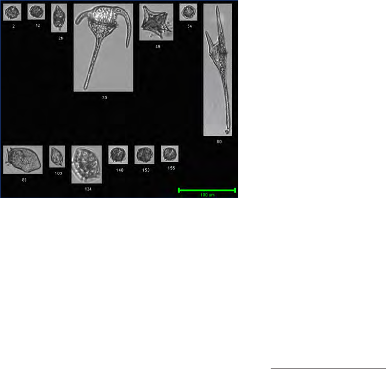
51
Microscopic and Molecular Methods for Quantitative Phytoplankton Analysis
Chapter 8 Imaging flow cytometry - FlowCAM
Flow Cell) before it runs dry. Preventing air from entering the
Flow Cell between samples will prevent tiny bubbles from
forming that could be detected as particles and imaged in the
next sample. Any clogs can be removed by reversing the pump
direction or inverting the Flow Cell and rinsing with FSW or
distilled water.
Data Analysis
Each fluorescent particle/cell is digitally acquired and archi-
ved by the FlowCAM ViSp software (Fig. 5). Analysis of the
samples is done either immediately upon completion of the
sample acquisition or at a later time after many samples have
been acquired or archived. The ViSp software allows the ope-
rator to use previously acquired image libraries of target spe-
cies or organisms to assist in sample analysis. The libraries
are user generated and can be created from images obtained
from cultured organisms or from positively identified natural
field images of the target organism. The libraries allow the
operator to pattern match each field sample by filtering and
sorting the data into user defined catagories. This procedure
can be repeated for different target organisms within a single
sample or multiple samples. Once the analysis is completed,
the positively identified images are verified by the operator,
and a total count of each class or group is determined. The
final cell concentration of each class is determined using an
equation that includes the cell count, volume analysed and
Flow Cell Factor – see Formula for Calculating Results below.
Calibration
Prior to microphytoplankton sample analysis, the FlowCAM
needs to be properly calibrated using an optical micrometer.
The micrometer is used to measure the field-of-view of the
camera for each magnification objective (4x & 10x), enabling
an accurate size calibration for each pixel. This ”calibration
factor” becomes part of the context settings for each mag-
nification. Prior to shipment, a new FlowCAM is calibrated
to assure accurate measurements of particle concentration
(particles/mL) and for sizing particles. Although no in-field
calibration is required, a FlowCAM user can analyse polysty-
rene or latex beads (of known size) for calibration assurance.
Calibration beads can be purchased at a variety of commercial
companies (10-100 µm, Duke Scientific, USA). To verify the
FlowCAM calibration refer to the FlowCAM Operators Ma-
nual for a detailed step by step protocol.
Preservation and storage
Unpreserved samples are ideal for quantifying and analysing
microphytoplankton in the field, and is recommended. Ho-
wever, this is not always appropriate. Preservation of samp-
les should be done using a 10% buffered formalin solution
or formalin:acetic acid, such that the final concentration is
approximately 1-2%. Preserved samples should be processed
as soon as possible, as fluorescence detection is essential for
accurate cell detection and enumeration. Chlorophyll fluo-
rescence within the cell decreases with prolonged storage.
Preserved samples are best analyzed using Auto Image Mode,
to assure accurate phytoplankton counts. However, more pro-
cessing time is required in this mode in order to analyze an
adequate sample volume. If longer preservation is required,
the effects of the storage length should be tested on the Flow-
CAM prior to processing samples on a routine basis.
Formulas for calculating results
To determine the concentration of the target microplankton
group or species within a sample three values are needed:
1 The volume processed by the FlowCAM;
2 The cell count of the target group (based on classifica-
tion) (N);
3 The Flow Cell Factor.
Since the camera on the FlowCAM can only visualise a por-
tion of the Flow Cell (usually between 33-95% - depending
on the objective and Flow Cell used) the Flow Cell Factor
takes into account the portion of the field of view that is not
visualised by the FlowCAM. The Flow Cell Factor will vary
depending on the objective/Flow Cell combination utilised.
The Flow Cell Factor is calculated automatically by the ViSp
software once the correct dimensions of the Flow Cell used
are provided by the user. Note that Fluid Imaging Technolo-
gies has recently developed a new Flow Cell design that elimi-
nates the need for Flow Cell Factor.
Discussion
The ability to automate the detection and counting of
micro phytoplankton in field samples is a huge advantage
for monitoring aquatic systems. With the development of
more automated techniques, such as the FlowCAM there is
a movement to employing more remote automated monito-
ring techniques. The FlowCAM, with further development,
could assist in water quality monitoring for both marine and
freshwater environments. The FlowCAM is ideally suited for
quantifying microphytoplankton between 20-300 µm in size
(however, smaller and larger particles can also be detected).
Cell classification using the FlowCAM ViSp software is best
used on species/groups of phytoplankton that have unique
cell characteristics, such as cell size, shape or colour. For ex-
Figure 5. Representative black and white FlowCAM images from a
field sample containing the following genera, Dinophysis, Alexan-
drium, Protocentrum and Ceratium.
−
mL
FactorCellFlow
sample of Volume
N count Cell
mLcells ion concentrat Cell
*
)(
) (
) (
1
=
−
mL
FactorCellFlow
sample of Volume
N count Cell
mLcells ion concentrat Cell
*
)(
) (
) (
1
=
IOC Manuals & Guides no 55
Chapter 8 Imaging flow cytometry - FlowCAM
52
ample, the genera Dinophysis, Ceratium, and Chaetoceros have
many distinctive morphological features which are easier to
classify than different species within the genus Alexandrium.
The FlowCAM is best used to examine a wide range of species
within one sample. It can be used as a monitoring tool for
coastal projects or in the laboratory, processing discrete samp-
les when needed. In order to best evaluate the instrument a
list of Advantages and Disadvantages of the FlowCAM met-
hod are provided below:
Advantages of the FlowCAM Method
1 The amount of manual labour required for sample pro-
cessing and handling is greatly reduced when using a
FlowCAM for microphytoplankton analysis. For discrete
sample analysis (as described in this chapter) the operator
is required to set up and begin a run, but will only oc-
casionally monitor the FlowCAM when it is running and
detecting particles;
2 The FlowCAM records a “non-biased” digital record of
every particle/cell within a specific size range (determined
by the operator) for further analysis using the FlowCAM
ViSp software. Using traditional microscope techniques,
the operator scans the slide and either seeks out the par-
ticles/cells of interest or identifies all the observed cells on
the slide. This may result in a biased analysis and count of
a sample (which depends on the operator’s attention to de-
tail and identification knowledge). The data generated by
the FlowCAM is archived and can be reanalysed by more
skilled individuals when problems arise or when different
analyses are required;
3 In addition to capturing an image for each particle detec-
ted by the FlowCAM, the software provides instant image
analysis on each particle , up to 30 different image para-
meters. For example, particle length, width, equivalent
spherical diameter (ESD), area-based spherical diameter
(ABD), fluorescence, time of flight and aspect ratio are
some of the the primary data measurements obtained. Gi-
ven the data provided, the operator can develop specific
algorithms or use previously determined algorithms from
the literature for values of interest such as bio-volume and
Carbon:Chlorophyll ratio depending on the needs of the
application or project;
4 The FlowCAM is portable. Even the benchtop model has
a relatively small foot-print (100 x 70 cm) and can be used
in the lab or at sea on board ships. The image capture sys-
tem prevents problems usually associated with vibration;
5 The FlowCAM allows for the visualisation and/or detec-
tion of a wide particle size range (1 µm – 1 mm equivalent
spherical diameter). To detect across this large size range a
series of objectives and flow cells would need to be used.
Based on the size of the target organism to be detected
(for example, Alexandrium), a 10 X objective with a 100
µm depth flow cell would be used. To examine smaller or
larger particles within a sample, other objectives and flow
cell combinations may need to be used.
Disadvantages and Drawbacks
1 In terms of cell identification it is essential to achieve the
best possible focus, otherwise the images will be blurry and
will be difficult to analyse;
2 Depending on the ecosystem that is being analysed the
phytoplankton cell size range may vary greatly. Each ob-
jective and Flow Cell size that can be used has a minimum
and maximum cell size range that’s possible (similar to the
limitations of microscopy). Therefore, to best identify all
phytoplankton within a given sample, two FlowCAM runs
may be required at two different magnifications. This de-
pends on what magnification is acceptable for cell iden-
tification. If cells are too large to pass through the Flow
Cell clogging may occur. Therefore, method development
at the beginning of a particular project is important. Ho-
wever, if only one particle/cell size is required and cell
identification is not necessary– one FlowCAM run may be
sufficent;
3 A limited number of preservation techniques for phyto-
plankton detection using fluorescent based triggering can
be used. To assure accurate cell concentrations using pre-
served samples Auto Image Mode is recommended, but
more processing time is required (1-2 hours). The best
method of preservation is 1-2% final concentration for-
malin. Preserved samples should be stored cold and in the
dark. Prior to processing let the samples acclimate to room
temperature. Lugol’s iodine or other iodine based preserva-
tion methods are not recommended for use with the Flow-
CAM as the fluorescence of the particles is lost and the
high contrast of the images makes it difficult to identify
different phytoplankton groups/genera;
4 In situations where cold samples are being analysed in high
humid environments (for example, samples of deep water
being analysed on board ships), condensation on the flow
cell may interfere with particle detection. The solution to
this problem is to allow the sample to attain room tempe-
rature prior to analysis. The sample should be preserved
prior to manipulation;
5 When the particle load is very high as in riverine samples
containing high concentrations of detritus, more than one
particle may be captured in a single field of view on the ca-
mera using Trigger Mode. Although each particle will have
different image analysis values, such as particle length,
width, ESD etc., the fluorescent value of both particles will
be the same. It is also possible to capture “non-fluorescent”
material if the particle load (sediment) is too high and the
instrument is detecting particles in fluorescent detection
mode. In these cases, Auto Image Mode could be utilised;
6 The operator or user should have some knowledge of phy-
toplankton identification for analysis of the FlowCAM
data.

53
Microscopic and Molecular Methods for Quantitative Phytoplankton Analysis
Chapter 8 Imaging flow cytometry - FlowCAM
Type of training required to operate a FlowCAM
1 To perform sample analysis: Approximately one-two days
of training would be required with guidance from a trained
individual and follow-up support;
2 To troubleshoot and QC: A more experienced analyst
with up to 6 months experience would be more effecti-
ve at troubleshooting the instrument. The company that
manufactures the FlowCAM, Fluid Imaging Technologies
provides on-site, web-based, and over the phone customer
assistance when needed.
Acknowledgements
We would like to thank the support of Fluid Imaging Tech-
nologies who kindly provided assistance and pictures, specifi-
cally, Harry Nelson, Brian Thompson, Jonathan Villeneuve,
Gerald Brown and Doug Phinney. We also thank Murielle
LeGresley for comments and suggestions to the manuscript.
References
Anonymous (2009). FlowCAM Operators Manual, Fluid Imaging
Technologies, Inc., March 2009 Revision 0109.
Buskey, E . and Hyatt CJ (2006) Use of the FlowCAM for semi-
automated recognition and enumeration of red tide cells (Karenia
brevis) in natural plankton samples. Harmful Algae 5:685-692
Sieracki CK, Sieracki M and Yentsch CS (1998) An imaging-in-flow
system for automated analysis of marine microplankton. Marine
Ecology Progress Series 168: 285-296
Zarauz L, Irigoien X, and Fernandes JA (2009) Changes in plank-
ton size structure and composition, during the generation of a
phytoplankton bloom in the central Canatabrian sea. Journal of
Plankton Research 2: 193-207
Materials
Paraformaldehyde powder
1N NaOH
Stirring/hot plate
Chemical fume hood
pH meter
Phosphate buffer ed saline (PBS) or filtered seawater
Distilled H
2
O
G/F filters
1 Mix 900 mL distilled water and 100 g paraformaldehyde powder;
2 Set up on a stirring/hot plate under hood. Heat to approximately 60
º
C. Do not boil;
3 Stir for approx 1 hour. Turn off heat;
4 Add 100 µL 1N NaOH to “clear” solution. Cool to room temperature. Note: In some cases, not all the paraformaldehyde will go into
solution;
5 Add 100 mL phosphate buffered solution or filtered seawater. , depending on whether the samples are freshwater or marine;
6 Filter through GF/F filter to remove precipitate;
7 Test pH. Should be 7.4 - 8.0 (approx. equal to seawater);
8 If necessary, add more NaOH.
This yields a 10% solution (approximately).
Preparation of a Formalin: Acetic Acid Solution
Materials
Formaldehyde (37%)
Concentrated acetic acid
1 Mix equal parts of formaldehyde and acetic acid;
2 Using this solution, add 2.5 mL per 100 mL of sample.
Appendix 1
Preparation of a Buffered Paraformaldehyde/Formalin Solution

IOC Manuals & Guides no 55
Chapter 8 Imaging flow cytometry - FlowCAM
54
Equipment Supplier Cat. Number
€
US $
FlowCAM
VS IV Fluid Imaging Technologies
(FIT), USA
VS IV or portable VS IV 53,760 80,000
50um Flow Cell FIT, USA FC50 28 41
100um Flow Cell FIT, USA FC100 19 28
300um Flow Cell FIT, USA FC 300 19 28
Nylon Mesh Wildco, USA www.wildco.com 24-C27 (53 µm)
24-C34 (100 µm)
24-C48 (300 µm)
89 132
Silicone Tubing (1.6
mm ID)
Cole Palmer, USA K-06411-62 12 18
Calibration Beads Duke Scientific, USA
www.dukesci.com
4205A (5 µm diameter)
4210A (10 µm diameter)
4220A (20 µm diameter)
4250A (50 µm diameter)
4310A (100 µm diameter)
623 927
Plastic Pipets VWR, USA 14670-103 36 53
Mini-funnel Hutzler Manufacturing
www.usplastic.com
801 0.67 1
Paraformaldehyde VWR, USA MK262159 38 56
Sum approx.
54,536 81,284
Appendix 2
Table 1. Equipment and costs..
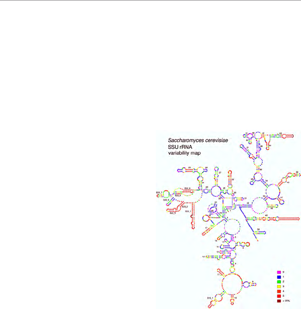
55
Microscopic and Molecular Methods for Quantitative Phytoplankton Analysis
Chapter 9 Whole cell hybridisation assays
Introduction
Fluorescence in situ Hybridisation (FISH)
Ribosomes are the sites for protein synthesis in all cells. All
cells are packed with many ribosomes because protein synthe-
sis is an on-going cellular process. Each ribosome is composed
of ribosomal RNAs (rRNAs) and accompanying proteins.
The RNAs within the ribosome fold into a shape that permits
the synthesis of the proteins and this folding of the molecule
is maintained for proper functioning of the ribosome. If mu-
tations occur that violate the folding of the molecule, then the
molecule is non-functional. Within the interior of the folded
RNA is the conserved sequence regions. These cannot change
otherwise the molecule will not fold properly. The more vari-
able regions of the RNA molecule are found on the surface of
the molecule which do not interfere with the folding of the
molecule. Thus, based upon conserved and variable regions of
the rRNA, signature base sequences of varying taxonomic spe-
cificity can be found (Fig. 1). In other words, regions can be
identified in the rRNAs that will recognise all members from
as broad a group as a kingdom of organisms or be so selective
to identify only a species or cluster of strains in that species.
These short sequences have been used to develop probes for
the identification of organisms at various taxonomic levels.
Given the vast amount of rapidly accumulating sequence data
for all kinds of organisms, it is now possible to develop these
probes for a broad spectrum of taxa. When these probes are
coupled with a fluorescent marker, the target organism can
be easily identified by a technique known as Fluorescence in
situ Hybridisation (FISH). Fluorescence in situ hybridisa-
tion enables the rapid detection of different species or strains
(Amann 1995). This technique has been successfully applied
for the detection of harmful algae (Anderson 1995, Miller
and Scholin 1996, 2000, John et al. 2003, Anderson et al.
2005) as well as algal classes (Simon et al. 1997, 2000, Rhodes
et al. 2004a, 2004b, Eller et al. 2007) and other taxonomic
hierarchies (Groben et al. 2004, Groben and Medlin 2005,
Töbe et al. 2006).
Basic Principles of FISH
The target algal cells are hybridised with fluorescently (e.g.
the fluorochrome fluorescein isothiocyanate; FITC) labelled
oligonucleotide probes, which bind to the complementary
target sequence of the rRNA in the ribosomes (Fig. 2). This
results in a bright labelling of the entire algal cell because of
the high target number of ribosomes in cells (Figs. 2-4). A list
of all algal probes can be found on the EU PICODIV (Di-
versity of Picoeukaryotic Organisms) website (http://www.
sb-roscoff.fr/Phyto/PICODIV/). In each RNA molecule the
more conserved positions can be used to develop taxonomic
probes e.g. on a class level, whereas the variable regions are
used for lower taxonomic levels.
Initially, the cells are fixed with a preservative that actually
makes the cell membrane permeable for the entry of the
probe into the cell. The fluorescently labelled probe finds its
way to the ribosome and binds to the region of the rRNA
to which it is complementary, forming a duplex. When the
sample is viewed under a fluorescent microscope using light
of the correct wavelength, the fluorochrome is excited and
the cell of interest can easily be visualised. The three methods
described in this chapter all incorporate these basic principles
of FISH; however, there are slight variations in their protocols
9 Detecting intact algal cells with whole
cell hybridisation assays
Kerstin Töbe*
1
, David Kulis
2
, Donald M. Anderson
2
, Melissa Gladstone
3
, and
Linda K. Medlin
4
1
Alfred Wegener Institute for Polar and Marine Research Am Handelshafen 12. D-27570 Bremerhaven, Germany
2
Biology Department, MS #32, Woods Hole Oceanographic Institution, Woods Hole, MA 02543, USA
3
Cawthron Laboratory Services, Cawthron University, Private Bag 2, Nelson, New Zealand
4
Observatoire Océanologique de Banyuls-sur-Mer, Laboratoire Arago, 66651 Banyuls-sur-Mer, France
*Author for correspondence e-mail: Kerstin.T[email protected]
Figure 1. Variability map of the 18S rRNA molecule. Source:
Bioinformatics.psb.ugent.be.

IOC Manuals & Guides no 55
Chapter 9 Whole cell hybridisation assays
56
Scope
Detection and quantification of target phytoplankton species.
Detection range
Detection of microalgal RNA by FISH is very sensitive. The
number of cells that can be detected depend on the sample vo-
lume. High biomass can obscure the view of target cells.
Advantages
Relatively inexpensive if appropriate fluorescence micrsocopy
facilities are available. Visible observation of cells is possible.
Simple and easy to use. Sample volumes can easily be adjusted.
Simultaneous labeling and detection of multiple species is pos-
sible.
Drawbacks
Probes are only available for a limited number of target species.
Rigorous optimisation and specificity testing on local strains is
required before the method can be implemented. Finite storage
time for samples. Processing procedure may result in cell loss.
Relatively expensive start-up costs. Intensity of the positive
reaction may vary with cell conditions. Access to molecular ex-
pertise is essential. Appropriate laboratory facilities for storage
and processing of probes and reagents are necessary.
Type of training needed
Instruction in setting up this technique should come from a
person with an in-depth knowledge and experience of mole-
cular biology. Approximately one week of supervised training
required to properly perform the method.
Essential Equipment
Epifluorescence microscope, filtration unit, hybridisation oven,
various air displacement pipettes, vacuum pump.
Equipment cost*
Total set-up cost = 20000 € (30000 US $)
See Appendix, Table 1 for details.
Consumables, cost per sample**
Cost per sample = 1.67 € (2.50 US $). See Appendix, Table 2
for details.
Processing time per sample before analysis
In total ca. 4 hours per sample. This excludes fixation time
which is 1-24 hours.
Analysis time per sample
Microscopical analysis 45 minutes to 2.5 hours/sample.
Sample throughput per person per day
A trained person can process and count 16 or more samples/
day.
No. of samples processed in parallel
Number of samples processed in parallel: 14-24 (dependent
upon manifold capacity).
Health and Safety issues
Formamide, formalin, methanol and DAPI are hazardous
chemicals. Proper safety guidelines should be employed when
using them - lab coat, eye protection and gloves are required.
Disposal of all waste products should follow prescribed labo-
ratory procedures. Continual microscope work could result in
strain injury. It is important to incorporate breaks into the daily
analyses time. Ergonomic adjustments to the microscope and
the working place is recommended.
*service contracts not included
**salaries not included
The fundamentals of
The fluorescent in situ hybridisation (FISH) method
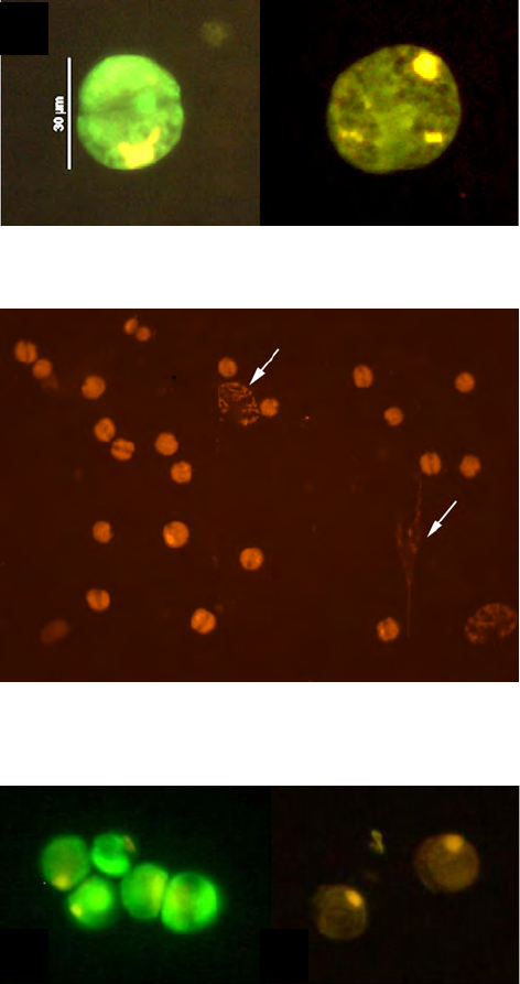
57
Microscopic and Molecular Methods for Quantitative Phytoplankton Analysis
Chapter 9 Whole cell hybridisation assays
that offer the user various advantages depending upon their
specific sample requirements. Optimisation of the FISH assay
is required for each new probe/probe set and should involve
testing a matrix of conditions including:
• Hybridisation buffer - 1X, 5X, respectively, depending on
the protocol used. Set buffer and if required, 5% intervals
of formamide concentrations. See Appendix, Table 3 for
more details on how to make up the different buffers
• Hybridisation length - longer hybridisation times can re-
sult in non-specific binding
• Hybridisation temperature - low temperatures can cause
non-specific binding and temperatures that are too high
may inhibit binding
• Hybridisation wash buffer and wash duration – these
steps influence the intensity of the target label as well the
degree of non-specific labelling
The strongest positive signal from the target organism and
lowest cross reactivity from non-target organisms will define
the optimal assay conditions for the probe.
Materials
Laboratory Facilities
This method can be used in laboratories and on board re-
search vessels.
Required Equipment (essential)
The whole cell method requires the following equipment:
• Epifluorescence microscope
• Filtration manifold
• Hybridisation oven or water bath with thermometer
• Air displacement pipettes (10 µL – 10 mL)
Equipment, Chemicals and Consumables
The equipment, chemicals and consumables used in this
method are presented in the Appendix, Tabels 1-2 at the end
of this chapter. Suppliers, catalogue numbers and estimated
cost in Euros and US Dollars for the year 2007 are also listed
in Appendix.
Method
Three different fluorescence in situ hybridisation
(FISH) methods are presented. Method 1 and 3 use
the LSU probe, NA1, recognising the North Ameri-
can Alexandrium ribotypes (Alexandrium fundyense
/catenella/tamarense) 5’-Fluor/AGTGCAACACTCCCACCA
-3’ (Anderson et al. 1999). In method 2 another LSU probe,
NA2, which also discriminates North American ribotypes
was used: 5’-Fluor/ AACACTCCCACCAAGCAA -3’ (John
et al. 2003). This probe has a 5 bp (base pair) shift of NA1
sequence to avoid the hair pin loop that this probe makes
with itself that might reduce its hybridisation ability at low
temperature.
Methods 1-3 below are variations of the FISH assay using Al-
exandrium fundyense as the target organism. Each method dif-
fers slightly according to different personal preferences with
regards to some of the equipment used, preservation methods
and the hybridisation protocol (see Table 1 for more details).
With the appropriate filtration set, many samples can be
processed in parallel. Samples in methods 1 and 2 can be eas-
ily filtered overnight for processing in the morning with probe
hybridisation. It is preferable that no significant delays oc-
cur during the sample processing steps when using method
3. With any of the methods, the hybridisation takes approxi-
mately 2 hours and the filters can be enumerated thereafter.
The number of samples to be processed and counted will vary
with each worker; the majority of time is devoted to micro-
scopic examination of the sample. The time spent on each
sample varies depending upon the target cell density, the con-
centration of non- target cells, detrital matter and counting
method employed. The reader is referred to chapter 14 on
the laser scanning cytometer to avoid personal examination
of the filters.
Figure 2. Micrographs of Alexandrium fundyense cells using the
FISH method: A FISH with FITC-labelled probe NA1 (Miller and
Scholin 1998); B Negative control, no probe. 400X.
Figure 3. Fluorescence in situ hybridisation with Alexandrium
fundyense cells with Cy3-labelled probe NA1. Note the autofluo-
rescence of the dinoflagellate cells of the genera Dinophysis and
Ceratium in the background (arrows) 200X.
Figure 4. In-Stu Hybridisation with Alexandrium ostenfeldii cells: A
FISH with FITC-labelled probe Aost (John et al. 2003). B Negative
control, no probe. 400X. Cawthron laboratory.
A B
A B

IOC Manuals & Guides no 55
Chapter 9 Whole cell hybridisation assays
58
Method 1
Materials
Solutions for Fixatives
• Modified Saline Ethanol Solution (Miller and Scholin
2000; see Appendix, Table 3 for details).
This fixative is stable at room temperature for several months
without precipitate formation. Note: 300 mL of fixative is
sufficient for approximately 70 reactions. The modified sa-
line ethanol does not form precipitates and can be made in
advance, whereas the unmodified version with a higher etha-
nol concentration forms precipitates and should be made just
before use.
• 25X SET buffer (discard after 12 months; see Appendix,
Table 3 for details)
Solutions for Fluorescence in situ Hybridisation
The hybridisation buffer concentration needs to be optimised
for each probe set (see the discussion in ‘Basic Principles of
FISH’).
• 1X SET buffer (used for dinoflagellates from the genera
Karenia and Alexandrium; see Appendix, Table 3 for de-
tails)
or
• 5X SET buffer (used for diatoms from the genus Pseudo-
nitzschia; see Appendix, Table 3 for details)
• Mix solutions into a baked 500 mL Duran bottle and
filter through a 0.45 µm filter. Add 1 mL Polyadenalyic
acid (12.5 mg mL
-1
, Sigma Chemical, P-9403)
• Wash buffer: 1X SET buffer (see Appendix, Table 3 for
details) in sterile Milli-Q water
Probes
Probes are received as a dried powder and need to be made up
to a concentration of 200 ng µL
-1
i.e. 50 µg of probe in 250
µL of 1X TE buffer, pH 7.8- 8.0. Make sure all equipment
is RNase free and the area is in dim light. Divide into 50 µL
aliquots and store at 4 ºC. Probes stored this way will remain
stable for 4 months, otherwise, samples need to be lyophilised
and stored at -80 ºC for long term storage.
Additional Equipment
• Milleriser Rig (includes tubes, bases, o-rings, lids)
• Water bath with heater and thermometer
• Hand held vacuum pump and trap
• 2-20 µL micropipette + sterile tips
• 100 - 1000 µL micropipette + sterile tips
• 1-10 mL pipette + sterile tips
• Glassware (including Duran bottles) baked for 4 hours at
160 °C
• Latex disposable gloves
• Glass slides
• 22 mm x 22 mm glass cover slips
• Fine tip tweezers
• 500 mL volumetric flasks, acid washed in 3N HCl
• Poretics Polycarbonate filters; 3.0 µm pore size; 13 mm
diameter (Osmonics Inc.). Note that 5-8 µm pore size
filters can be used for larger cells
• Slowfade® Gold antifade reagent (Molecular Probes, In-
vitrogen Detection Technologies, S36936)
Fixation
1 Gloves must be worn at all times to avoid contamination
of samples with human derived RNAases;
2 Switch water bath heater on, set at 45 ºC;
3 Set up Milleriser Rig (Fig. 5). Assemble one filter set for
each species specific probe, plus a positive control, SSU-
targeted universally conserved sequence (Embley et al.
1992, Field et al. 1988), a negative control (the comple-
ment of UniC) and a ‘no probe’ control;
4 Using tweezers, place the o-ring into the tube. Place a
filter onto the o-ring ensuring that the shiny side faces
the sample. Screw the base into tube and tighten until
finger tight. Do not over tighten. Place assembled tube
into Milleriser Rig. Attach tube of vacuum trap flask to
the Milleriser Rig and tube of vacuum pump to outside
flask outlet;
5 Ensure valves are closed (i.e. horizontal);
Differences between methods Advantages Disadvantages
Method 1 Method 2 Method 3
Fixative Saline ethanol Saline ethanol Formaldehyde
with methanol
extraction
Formaldehyde/methanol
allows long term storage
of samples (> 1 year @
-20 ºC)
Use of hazardous
chemicals and an extra
centrifugation step
Saline ethanol is not
hazardous
Hybridisation buffer 5X or 1X Set
Buffer
5X SET Buffer with
Formamide
5X SET Buffer with
Formamide
Use of an hazardous
chemical
Wash buffer 1X Set Buffer 1X Set Buffer 0.2X Set buffer Method 1 does not require
a separate wash solution
for dinoflagellates.
Equipment Water bath Hybridisation oven Hybridisation oven Water bath is not very
expensive
A water bath is
cumbersome to work with
A hybridisation oven is
easy to use
A hybridisation oven is
more expensive
Table 1. Summary of the differences, advantages and disadvantages between the three methods discussed in this chapter.
59
Microscopic and Molecular Methods for Quantitative Phytoplankton Analysis
Chapter 9 Whole cell hybridisation assays
6 Live field samples: Add 5 mL saline ethanol fixative to
each tube. Add live sample to the fixative. Use 5-10 mL
of field sample (the volume can be varied according to
cell numbers present). Filter down to 3 mL and add a
further 3 mL of saline ethanol fixative;
7 Lugol’s iodine treated samples: add 5 mL saline etha-
nol fixative to each tube. Add 10 mL of Lugols treated
sample to the saline ethanol fixative. Add 3 drops of 3%
Sodium thiosulphate (decolouriser) to each tube using a
Pasteur pipette;
8 Cap tubes and tap gently to ensure no air bubbles are sit-
ting on the filter. Let the sample stand for 1 to 24 hours,
occasionally tapping gently to remove any air bubbles;
9 Filter fixed samples ensuring the solution level does not
drop below the level of the gasket. Do not let pressure
gauge read over 10 mgHg. Fixed samples can be kept for
up to 4 weeks when stored at 4 ºC.
Fluorescence in situ hybridisation
10 Add 2 mL 1X SET hybridisation buffer to each tube;
11 Filter samples as above - do not let filters dry out;
12 Add 0.5 mL 1X SET hybridisation buffer to each tube;
13 Darken room as much as possible for following steps as
probes are light sensitive;
14 Add 12 µL (final concentration in hybridisation 4.8 ng
µL
-1
) probe to tubes. Gently mix the pipette tip in the
hybridisation buffer taking care not to touch the filter;
15 Put lids on tubes. Place the Milleriser Rig and tubes in
a water bath, ensuring that the solution in the tubes is
covered by the water level. Cover water bath with lid (or
aluminium foil) to prevent light exposure. Leave in water
bath for 1 hour;
16 Remove from water bath and filter as above;
17 Add 2 mL 1X SET hybridisation buffer and leave at
room temperature for a few minutes;
18 Gently filter samples until dry;
19 One by one disassemble tubes, remove filters using twee-
zers and place on labelled slides;
20 Pipette 12 µL of Slowfade® Gold antifade reagent onto
each filter and add coverslip;
21 Keep slides covered (i.e. in the dark) until they are ready
to be viewed. Colour reaction is enhanced if slides are left
to sit in the dark for about 30 minutes before analysing;
22 Analyse slides using an epifluorescence microscope (exci-
tation 490 nm; emission 520 nm) at 200X magnification
(Fig. 4);
23 Cells fluoresce brightly if the probe hybridises with tar-
get rRNA. This defines a positive result. Species-specific
probe filters need to be compared with the positive, nega-
tive and ‘no probe’ controls to discriminate positive fluo-
rescence from autofluorescence exhibited by non-target
cells;
24 Results may be recorded as a comment based on the inten-
sity of colour and the pattern of fluorescence. For example:
”++” indicates a strong positive result, where cells
are very brightly coloured with the flurochrome
”+” indicates a positive result or positive cells present.
”-” indicates no cells are showing a positive result, cells
may have a natural orange autofluorescence;
25 Cells should be counted after an initial examination of
each filter. Positive cells on the positive control filter must
be counted as well as cells on all the species filters;
Method 2
Materials
Solutions for fixation
Saline ethanol (Scholin et al. 1996; see Appendix, Table 3 for
details), prepared freshly for each experiment because of the
formation of precipitates or modified saline ethanol (Miller
and Scholin 2000; see Appendix, Table 3 for details) as de-
scribed in method one.
Solutions for Fluorescence in situ hybridisation
• Hybridisation buffer
• 5X SET buffer (see Appendix, Table 3 for details)
• 0.1 % (v/v) Nonidet-P40
• x % (v/v) Formamide*
*Note: Formamide concentrations must be determined for
every single probe by performing FISH assays with forma-
mide concentrations in 5 % intervals and microscopically ver-
ified. The appropriate formamide concentration will brightly
label all of the target cells tested with no cross hybridisation.
The formamide addition will reduce the binding temperature
of the probe so that it can hybridise specifically at 50 ºC. The
hybridisation buffer should be filter sterilised if stored for a
longer time.
Wash buffer
• 1X SET buffer (see Appendix, Table 3 for details) in ste-Table 3 for details) in ste-for details) in ste-
rile Milli-Q water
Probes
Fluorescently labelled probes purchased from Thermo Scien-
tific, Germany are delivered lyophilised. Stock solution of 1 µg
µL
-1
should be prepared and working solutions of 500 µL
-1
and
50 ng µL
-1
in 1X TE buffer, pH 7.8- 8.0. Probe stock solution
should be stored at -80°C and working solutions at -20°C.
Additional Equipment
• Filter vacuum manifold (Millipore, Bedford, USA) or
glass filter equipment
• Hybridisation oven
• Vacuum pump
• Pipettes 1-20 µL, 100-100 µL + sterile tips
• 1-50 mL pipette + sterile tips
• Autoclaved glassware
• Disposable gloves
• Glass slides
• Coverslips
• Tweezer
• White polycarbonate filter membranes: 47 mm or 25
mm diameter, pore size depending on cell size (Millipore,
Bedford, USA)
• DAPI (4’-6-Diamidino-2-phenylindole, Invitrogen,
Karlsruhe, Germany)
• Citifluor (Citifluor Ltd., Cambridge, UK)
• Colourless nail varnish
Fixation
1 Filter approximately 5 mL sample down onto a polycar-
bonate filter with the lowest possible vacuum and incuba-
te in the fixative for at least 1 hour at room temperature
or overnight at 4 ºC;
2 Incubate the filter for 5 minutes with hybridisation buffer
at room temperature to avoid precipitation. Air dry the
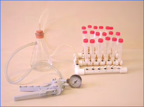
IOC Manuals & Guides no 55
Chapter 9 Whole cell hybridisation assays
60
filter and use directly for FISH. Alternatively the filter can
be stored at room temperature for at least 1 month.
Filters can also be cut in several pieces and treated individu-
ally for the detection of additional algal species in one sample.
This has to be taken into account when calculating the final
cell density.
Fluorescence in situ Hybridisation
3 Apply 60 µL of hybridisation buffer containing the la-
belled probe onto the filter and hybridise for 2 h in the
dark at 50°C. The final probe concentration in the buffer
should be 5 ng µL
-1
. Controls are espeically recommen-
ded for newly designed probes. These should include (1)
A ’no probe’ control: the same procedure without the ad-
dition of a probe. (2) A ’positive control’ where a known
working probe is used. (3) A ’negative hybridisation con-
trol’ where a ’nonsense’ probe is used which would not
bind to any of the cells because of its target sequence;
4 Place the slide in a darkened box with moistened filter
paper to provide a humid chamber for the hybridisation
to take place. The hybridisation temperature is kept at
50°C for all probes as the thermal melting point of the
probe is compensated by the addition of formamide to en-
hance the specificity of each probe. Readers are referred to
Amann (1995) and Groben and Medlin (2005) for a full
description of how probes should be developed. It is im-
portant to ensure that the entire filter piece is covered with
liquid and if necessary, more buffer-probe mixture should
be used. The fluorescently labelled probe is light sensitive,
so the filters should be kept in the dark for the rest of the
procedure, i.e. cover them during incubation times and
minimise exposure to light when they are handled;
5 Terminate hybridisation by washing the filters in pre-
warmed (50 ºC) 1X SET wash buffer for 10 minutes
at 50 ºC. After washing, dry the filters by blotting onto
Whatman filter paper.
Counterstaining and Validation using Microscopy
6 Mix one mL of Citifluor antifade + 0.5 mL Milli-Q water
+ 1.5 µL DAPI (1 µg µL
-1
);
7 Place the filters on a glass slide; two filters, 25 mm in dia-
meter, can be placed side by side on one glass slide. Add 60
µL DAPI/Citifluor mixture to the filters, place a cover slip
over the filters and seal edges with nail varnish. Store slides
in the dark until examined. Slides can be kept frozen for
several months without loosing fluorescence signal;
8 Analyse by epifluorescent microscopy using the appro-
priate filter set for the fluorochrome attached to the probe
(Fig. 2). When bound to the rRNA of target cells, positive
labelled cells fluoresce bright and are counted as positive
signal. Also the intensity of the given fluorescence has to
be recorded. The presumed positive results must be com-
pared with positive, negative and ’no probe’ controls to
differentiate between a real signal from the bound probe
and nonspecific binding of probes or autofluoresence.
Method 3
Materials
Solutions for Fixation
• Formaldehyde, 37% (Fisher Scientific, F79P-4)
• 100% ice-cold methanol (Fisher Scientific, A452SK-4)
Solutions for Fluorescence in situ hybridisation
• 25X SET buffer (as described in the Appendix, Table 3)
• 5X SET Hybridisation buffer (to process 14 samples)
20.4 mL Milli-Q water
6.0 mL 25X SET buffer
300 µL Igepal CA-630 (Sigma Chemical, I 3021)
300 µL Polyadenylic acid (poly A) 10 mg mL L
-1
(Sigma Chemical, P 9403)
3.0 mL Super Pure Formamide
(Fisher Scientific, BP228-100)
Probes
For the North American Alexandrium ribotypes (Alexandrium
fundyense/catenella/tamarense) the NA1 oligonucleotide probe
can be used: 5’-Fluor/ AGTGCAACACTCCCACCA -3’
(Anderson et al. 1999). Probe stocks should be stored in dry
100 µg aliquots at -80 ºC. Resuspend probe stocks in 500
µL 1x TE [TE-Tris-EDTA buffer 100X concentrate (Sigma
Chemical, T-9285); working stock 200. Add 360 µL of resus-
pended probe to 15 mL hybridisation buffer for incubations.
• Wash buffer (0.2X SET)
120 µL 25X SET buffer
14.880 mL Milli-Q water
Additional Equipment
• Filter vacuum manifold (Promega Corp., A7231) with
custom made 25 mm filter funnels, (modification of the
ones described by Scholin et al. (1997) and are similar to
those in Figure 5)
• Filter membranes: 25 mm Cyclopore membrane (What-
man Inc., 5 mm pore size, 09-930-14E)
• ProLong Gold antifade reagent (Molecular Probes, Invi-
trogen Detection Technologies, P36930)
Fixation
1 Preserve a 14 mL sample with 0.75 mL formaldehyde
(5% v/v, final concentration = 1.9% formaldehyde) in a
disposable 15 mL centrifuge tube;
2 The 14 mL volume may be a raw water sample or a con-
centrated sample generated using filtration;
3 In the field, 2-4 lof water is typically filtered through a 20
µm Nitex sieve (Nitex mesh, Sefar America, Inc., fitted at
the end of a 3 in. diameter PVC tube) and the collected
Figure 5. Custom made Milleriser Rig.

61
Microscopic and Molecular Methods for Quantitative Phytoplankton Analysis
Chapter 9 Whole cell hybridisation assays
cell material is resuspended to the 14 mL mark and pre-
served with 5% v/v formalin;
4 Store the samples at 4 ºC for a maximum of 36 hours
until they can be centrifuged at 3000 x g, for 5 minutes
at room temperature;
5 Aspirate the supernatant and resuspend the cell pellet in
14 mL of ice-cold methanol to extract the chlorophyll
and to stabilise the rRNA. Samples are required to stand
in methanol for at least 1 hour prior to hybridisation but
are stable for many months when stored at -20 ºC.
Fluorescence in situ Hybridisation
6 Add a volume of sample to a filter funnel containing a
Cyclopore filter. Filter the sample to near dryness using
the lowest possible vacuum;
7 Add 1 mL of pre-hybridisation buffer and incubate for
5 minutes at room temperature. Note: The filter funnel
valves should only be open when filtering; they should
remain closed at all other times;
8 Filter the pre-hybridisation buffer and add 1 mL hybridi-
sation buffer with added probe. Cap the filter tubes and
place the manifold in a black plastic bag. The bag should
contain several wet paper towels to provide a humid envi-
ronment. Seal the bag and place the samples in a dry heat
incubator at 50 ºC (±2 ºC ) for 1 hour;
9 Complete the hybridisation reaction by filtering the
hybridisation buffer plus probe and adding 1 mL pre-
warmed (50 ºC) 0.2X SET wash buffer. Allow this to
incubate for 5 minutes at room temperature;
10 Filter the wash buffer. Keep the filter funnel valve open
and continue to apply vacuum to the sample until the
filter has been placed onto a microscope slide. Add 25
µL ProLong Gold antifade reagent and a coverslip to the
filter. Samples can be stored at 4 ºC in the dark for several
weeks prior to observation, but, best results are obtained
by viewing the sample immediately after hybridisation;
11 Samples can be observed and counted with epifluores-
cence microscopy, at 100X using the appropriate filter
set. For Cy3, Chroma 41032 or FITC, Chroma 41012
(Chroma Technology Corp.) filter sets are recommended
(Fig. 3).
Formulas for Calculating Results
Ideally the entire filter is examined and positive cells enu-
merated.; hence, the cell number is reflective of amount of
original sample that was processed and preserved as well as to
the volume of the preserved sample that was placed onto the
filter for hybridisation. It should be noted, that only the filter
area is counted and not the entire area under the coverslip,
which is usually larger than that of the sample filter. If target
cell densities are high and warrant only counting a portion of
the filter, then a decision has to be made on how to proceed
with the count to afford a statistically reliable value. Andersen
and Throndsen (2004) provide a good review on this in their
chapter in the Manual on Harmful Marine Microalgae.
A generic formula to calculate cells L
-1
for all 3 methods:
where N is the number of positive cells on the whole filter and
V (mL) is the volume of sample used.
To calculate species composition of a bloom
The FISH assay can be used as a secondary test to light mi-
croscopy analysis when a designated cell count for a particular
genus (e.g. Pseudo-nitzschia) has been exceeded and speciation
is required to determine risk associated with toxicity. In cases
where the cell count has been determined previously for the
target genus, the percentage that each species comprises in
the sample (i.e. the total species positive counts) can be deter-
mined using the following formula:
where S is the number of positive cells on a species-specific
filter and T is the total number of genus positive counts.
Percentages calculated from the FISH data can be applied to
the original cell count to get an approximate density of each
species in the sample. Pieces of a filter can also be analysed.
Counts on the portion of the filter can be calibrated in a simi-
lar fashion to those of the Utermöhl method (chapter 2). This
removes the requirement for analysing the entire filter, pro-
vided that a sufficient proportion of a filter is analysed for
statistical significance and that the proportion is the same for
each species-specific filter.
Discussion
Whole cell, fluorescently labelled oligonucleotide enumera-
tion-based assays for HAB species can be a simple, effective
and efficient tool for counting natural phytoplankton sam-
ples. Empirical trials with more traditional counting methods,
as discussed in this manual and other studies (e.g. Anderson
et al. 2005), need to be conducted to determine the specifi-
city of the probe with the target species. This is because not
all species-specific probes will label morphologically identical
organisms because of their genetic dissimilarities. If a suitable
probe has been shown to hybridise with the target organism,
and the required equipment to perform the hybridisation
and subsequent microscopic analysis are available, then this
technique can easily be used to enumerate numerous samples
by researchers with limited laboratory and microscope experi-
ence. Automated counting systems, such as the ChemScan
(Chemunex, France), make this operation much faster (Töbe
et al. 2006).
The specificity that each probe binds to the target species
rRNA needs to be fully evaluated in optimisation and cross
reactivity trials. To optimise the FISH hybridization param-
eters for each probe, assay conditions such as reagent con-
centrations, hybridisation temperature and time can be ma-
nipulated to produce stronger epifluorescent signals. Methods
described in this manual (such as light microscopy and Cal-
cofluor staining), and in other studies, (e.g. Anderson et al.
2005) must be conducted to determine the extent (if any) of
cross reactivity with non-target species.
1000*
)(
)(
) (
1
−
mLsampleofVolume
NfilterwholeoncountcellPositive
LcellsionconcentratCell
1000*
)(
)(
) (
1
−
mLsampleofVolume
NfilterwholeoncountcellPositive
LcellsionconcentratCell
100 *
) (
) (
T filter whole on count cell genus Positive
S filter whole on count cell species Positive
ncompositiospeciesPercentage
100 *
) (
) (
T filter whole on count cell genus Positive
S filter whole on count cell species Positive
ncompositiospeciesPercentage
IOC Manuals & Guides no 55
Chapter 9 Whole cell hybridisation assays
62
Careful consideration must be given when determining the
assay conditions to balance signal intensity against cross reac-
tivity. Positive, negative and ‘no probe’ controls are critical for
this. Signal intensity of the target species compared with the
positive control will give an indication of optimal assay condi-
tions. The negative control will indicate non-specific binding
caused by sub-optimal conditions. The ‘no probe’ control is
critical for assessing the amount of autoflourescence exhibited
by the cells, which must not be confused as a positive signal.
Consideration also needs to be given to the choice of sample
preservation as two of the methods described herein utilise
the relatively safe ethanol/SET preservative, but, these do not
afford the luxury of long-term sample storage. Formalin fixa-
tion followed by methanol extraction and -20 ºC storage al-
lows for long-term sample archiving and subsequent hybridi-
sation, but, involves the use of hazardous chemicals and an
extra centrifugation step to remove the formalin seawater su-
pernatant from the cell pellet. Both fixation methods will pro-
vide the user with good labelling intensity of the target cells.
In New Zealand, the FISH assay is used as a supporting tool
to light microscopy providing additional information to regu-
lators. Multiple species-specific probes can be run as a screen
to determine the composition of a bloom when a sample has
returned elevated cell counts of potential species of concern.
The FISH assay enable rapid identification to the species level
in such cases; a task that would be both time consuming and
require a significant level of experience to achieve the same
results using light microscope techniques.
To increase cell detection limits for field samples, large vol-
umes of water (1-8 l) can be filtered through an appropriate
mesh size for concentration purposes, if the target organism
is amenable to this type of concentration (e.g. Anderson et al.
2005). The captured cell material can then be washed into a
centrifuge tube, preserved and an aliquot of the sample slurry
can then be processed for the FISH assay. One of the benefits
of using FISH is that samples with high biomass as well as
difficult to identify species can be easily examined and enu-
merated by an inexperienced microscopist. A 2 Litre sample
of field material can be concentrated down to a volume of 15
mL, of which, 7.5 mL is then processed for FISH affording a
limit of detection of 1 cell L
-1
. One Litre is more than suffi-
cient, unless the study, e.g. picoplankton, calls for greater vol-
umes. The sample volume used in the assay can be adjusted
based on cell counts derived from light microscope analysis
on test samples.
This method is suitable for all species for which a probe has
been designed and are amicable to the preservation methods
outlined here. The detection limit of one cell per filter can
easily be achieved by manual counts or if automatic counting
devices are used, such as the ChemScan solid phase cytometer
(see chapter 14 and Töbe et al. 2006). The accuracy of manual
counting depends on the amount of debris in the sample and
the skill of the microscopist to discriminate the positive signal
against the weak autofluorescence of other cells. In order to
ensure that the method works well, it is important that good
temperature control is achieved during the hybridisation step.
It is also imperative that the excess probe is washed off the
filter in order to reduce background fluorescent interference.
Acknowledgements
The work done by LKM and KT was funded by the Stif-
tung Alfred-Wegener-Institut für Polar und Meeresforschung
in the Helmholtz-Gesellschaft, Bremerhaven, Germany and
in part by EU DETAL, Project QLRT-1999-30778. Support
was provided by the following grants to DMA: the Univer-
sity of New Hampshire Cooperative Institute for Coastal and
Estuarine Technology (CICEET) as a subcontract through a
National Oceanic and Atmospheric Administration (NOAA)
Grant NA05NOS4191149; NSF (National Science Founda-
tion) Grant OCE-0136861 and the ECOHAB (The Ecol-
ogy and Oceanography of harmful Algal Blooms) program
through NOAA Grant NA16OP1438. This effort was sup-
ported in part by the U.S. ECOHAB program sponsored by
NOAA, the U.S. EPA (Environmental Protection Agency),
NSF, NASA (National Aeronautics and Space Administra-
tion) and ONR (Office of Naval Research) - ECOHAB con-
tribution number 323. Attendance at the workshop for Melis-
sa Gladstone was funded through the Technical Participation
Programme, New Zealand, and the New Zealand Food Safety
Authority.
References
Amann RI (1995) In situ identification of micro-organisms by whole
cell hybridisation with rRNA-targeted nucleic acid probes. In:
Akkermans ADL, van Elsas JD, de Bruijn FJ (eds) Molecular mi-
crobial ecology manual 336. Kluwer Academic Publishers, Dor-
drecht, NL, p. 1-15
Andersen P, Throndsen J (2004) Estimating cell numbers. In: Halle-
graeff GM, Anderson DM, Cembella A (eds), Manual on harmful
marine microalgae Intergovernmental Oceanographic Commis-
sion, UNESCO, Paris, France, p. 99-129
Anderson DM (1995) Identification of harmful algal species using
molecular probes: an emerging perspective. In: Lassus P, Arzul
Erard G, Gentien P, Marcaillou C, (eds) Harmful marine algal
blooms. Lavoisier, Intercept Ltd, p. 3-13
Anderson DM, Kulis DM, Keafer BA, Berdalet E (1999) Detection
of the toxic dinoflagellate Alexandrium fundyense (Dinophyceae)
with oligonucleotide and antibody probes: variability in labeling
intensity with physiological condition. J Phycol 35:870-883
Anderson DM, Kulis DM, Keafer BA, Gribble KE, Marin R, Scho-
lin CA (2005) Identification and enumeration of Alexandrium
spp. from the Gulf of Maine using molecular probes. Deep-Sea
Res II 52:2467-2490
Eller G., Töbe, K, and Medlin, L.K. (2007) A set of hierarchical
FISH probes for the Haptophyta and a division level probe for the
Heterokonta. Journal of Plankton Research, 29:629-640
Embley TM, Finlay BJ, Thomas RH, Dyal PL (1992) The use of
rRNA sequences and fluorescent probes to investigate the phylo-
genetic positions of the anaerobic ciliate Metopus palaeformis and
its archaeobacterial endosymbiont. J Gen Microbiol 138:1479-87
Field KG, Lane DJ, Giovanni SJ, Ghilselin MT, Raff EC, Pace NR,
Raff RA (1988) Molecular phylogeny of the animal kingdom. Sci-
ence. 239:748-53
Groben R, John U, Eller G, Lange M, Medlin LK (2004) Using fluo-
rescently-labelled rRNA probes for hierarchical estimation of phy-
toplankton diversity-a mini review. Nova Hedwigia 79:313-320
Groben R, Medlin LK (2005) In Situ Hybridisation of phytoplank-
ton using fluorescently labelled rRNA probes. In: Zimmer EA,
Roalson E (eds), Methods in enzymology. Elsevier, San Diego,
63
Microscopic and Molecular Methods for Quantitative Phytoplankton Analysis
Chapter 9 Whole cell hybridisation assays
CA. 395:29-310
John U, Cembella A, Hummert C, Ellbrächter M, Groben R, Med-
lin LK (2003) Discrimination of the toxigenic dinoflagellates
Alexandrium tamarense and A. ostenfeldii in co-occurring natural
populations from Scottish coastal waters. Eur J Phycol 38:25-40
Miller PE, Scholin CA (1996) Identification of cultured Pseudo-
nitzschia (Bacillariophyceae) using species specific LSU rRNA
targeted fluorescent probes. J Phycol 32:646-655
Miller PE, Scholin CA (1998) Identification and enumeration of
cultured and wild Pseudo-nitzschia (Bacillariophyceae) using
species-specific LSU rRNA-targeted fluorescent probes and filter
based whole cell hybridization. J Phycol 38: 371-382
Miller PE, Scholin CA (2000) On detection of Pseudo-nitzschia
(Bacillariophyceae) species using whole cell hybridization: Sample
fixation and stability. J Phycol 36:238-250
Rhodes L, Holland PT, McNabb P, Adamson J, Selwood AR (2004a)
Production of isodomoic acid C by Pseudo-nitzschia australis, as
determined by DNA probe and LC-MS technologies. In: Pro-
ceedings of HABTech03 Workshop, Nelson, November (2003)
Holland P, Rhodes L, Brown L (eds) Cawthron report No. 906,
p127. ISBN 0-476-00622-8
Rhodes L, Haywood A, Adamson J, Ponikla K, Scholin C (2004b)
DNA probes for the detection of Karenia species in New Zea-
land’s coastal waters. In: Steidinger K, Landsberg J, Vargo G (eds)
Harmful algae. (2002) Florida Fish and Wildlife Cons Comm,
Florida Inst Oceanography and IOC of UNESCO, p. 273-275
Scholin CA, Buck KR, BritschigT, Cangelosi G, Chavez FP (1996)
Identification of Pseudo-nitzschia australis (Bacillariophyceae) us-
ing rRNA-targeted probes in whole cell and sandwich hybridiza-
tion formats. Phycologia 35:190-197
Scholin C, Miller P, Buck K, Chavez F, Harris P, Haydock, P, Howard
J, Cangelosi G (1997) Detection and quantification of Pseudo-
nitzschia australis in cultured and natural populations using LSU
rRNA-targeted probes. Limnol Oceanogr 42: 1265–1272
Simon N, Brenner J, Edvardsen B, Medlin LK (1997) The identifi-
cation of Chrysochromulina and Prymnesium species (Haptophyta,
Prymnesiophyceae) using fluorescent or chemiluminescent oligo-
nucleotide probes: a means of improving studies on toxic algae.
Eur J Phycol 32:393-401
Simon N, Campbell L, Örnólfsdóttir E, Groben R, Guillou L, Lange
M, Medlin LK (2000) Oligonucleotide probes for the identifica-
tion of three algal groups by dot blot and fluorescent whole-cell
hybridisation. J Euk Micro 47:76-84
Töbe K, Eller G, Medlin LK (2006) Automated detection and enu-
meration of Prymnesium parvum (Haptophyta: Prymnesiophyc-
eae) by solid-phase cytometry. J Plankton Res 28:643-657

IOC Manuals & Guides no 55
Chapter 9 Whole cell hybridisation assays
64
Table 1. Equipment and Suppliers
Table 2. Chemicals and Suppliers
Appendix
Equipment Supplier Cat. Number € US $
Method
Filter Manifold Millipore XX2702550 400 587 2
Vacuum pump Omnilab 9.881 391 574 2,3
Incubator ”Shake’n’Stack” VWR 7996 2310 3387 2,3
Epifluorescence microscope, Eclipse
E800
Nikon MAA600BA 25000 36.654
2
Epifluorescence microscope,
Axioimager A1
Carl Zeiss 4300050000000000 16000 25000 1,3
Milleriser Rig Custom made 55 80 1
Waterbath Grant JBAqua-26 1130 1650 1
Filter Manifold Promega A7231 76 114 3
Pipette 2 µL – 20 µL Fisher Scientific 05-402-87 193 289 1,2,3
Pipette 20 µL – 200 µL Fisher Scientific 05-402-89 193 289 1,2,3
Pipette 200 µL – 1000 µL Fisher Scientific 05-402-90 193 289 1,2,3
Pipette 1 mL – 10 mL Fisher Scientific 05-403-121 193 289 1,2,3
Equipment Supplier Cat. Number
€
US $ Method
Fixation
Ethanol, absolute,1l Merck 1.009.832.500 73 107 1,2,3
Methanol, 100% Fisher Scientific A452SK-4 61 90 3
Milli-Q water Most labs have an in-house
supply
1,2,3
Sodium chloride, 1 kg Sigma-Aldrich S9888 23 34 1,2,3
Tris/HCl, 500 g Sigma-Aldrich T3253 96 141 1,2,3
Nonidet-P40, 100 mL Roche 11754599 74 109 2
EDTA, 500 g Sigma-Aldrich E7889 56 82 1,2,3
Formaldehyde, 37% Fisher Scientific F79P-500 27 40 3
Isopore white polycarbonate membrane filter, 3 µm pore size, Qty. 100 Millipore TSTP02500 130 191 2
Whatman,Cyclopore, 5 µm pore, 25 mm dia., Qty. 100 Whatman 7062-2513 67 100 3
Hybridisation
FITC-labelled probe Thermo Scientific - 65 95 2
FITC-labelled probe Oligos Etc. - 0.7* 1* 3
Igepal CA-630, 50 mL Sigma Chemical I3021 16 23 1,3
Polyadenylic acid (poly A) 10 mg/mL Sigma Chemical P-9403 29 42 1,3
Deionized formamide, 100 mL Sigma-Aldrich F 9037 46 67 2,3
Nonidet-P40, 100mL Roche 11754599 74 109 2
Counterstaining and microscopical validation
DAPI (4’-6-Diamidino-2-phenylindole) Invitrogen, Karlsruhe, Germany D1306 97 142 2
Slowfade® Gold antifade reagent Molecular Probes, Invitrogen
Detection Technologies
S36936 82 120 1
Citifluor antifade Citifluor Ltd., Cambridge, UK X506 117 172 2
ProLong Gold antifade reagent Molecular Probes, Invitrogen
Detection Technologies
P36930 71 104 3

65
Microscopic and Molecular Methods for Quantitative Phytoplankton Analysis
Chapter 9 Whole cell hybridisation assays
Solution/Reagent Purpose Contents
Modified Saline Ethanol Solution Fixative
(after Miller and Scholin 2000)
To make up 300 mL:
220 mL 22 vol. 95% ethanol
50 mL 5 vol. Milli-Q water
30 mL 3 vol. 25X SET buffer
Saline Ethanol Solution Fixative
(after Scholin et al. 1996)
To make up 300 mL:
250 mL 25 vol. 95% ethanol
20 mL 2 vol. Milli-Q water
30 mL 3 vol. 25X SET buffer
25X SET buffer Fixative
(discard after 12 months)
To make up:
219.15 g 3.75 M NaCl
157.60 g 0.5 M Tris/HCl , pH has to be near 8.0, before
adding EDTA
9.3 g 25 mM EDTA, pH 7.8, filter sterilised, 1 Litre
5X SET buffer Hybridisation buffer
(used for diatoms from the genus Pseudo-nitzschia)
To make up 400 mL:
316 mL Milli-Q Water
80 mL 25X SET buffer
4 mL 10% Igepal, CA-630 (Sigma Chemical, I 3021)
1X SET buffer Hybridisation buffer
(used for dinoflagellates from the genera Karenia
and Alexandrium)
To make up 400 mL:
380 mL Milli-Q Water
16 mL 25X SET buffer
4 mL 10% Igepal, CA-630
(Sigma Chemical, I 3021)
1X SET buffer, other use Wash buffer 1X SET buffer in sterile Milli-Q water
0.2X SET Wash buffer To process 14 samples:
120 µL 25X SET buffer
14.880 mL Milli-Q water
Table 3. Buffers and solutions
IOC Manuals & Guides no 55
66
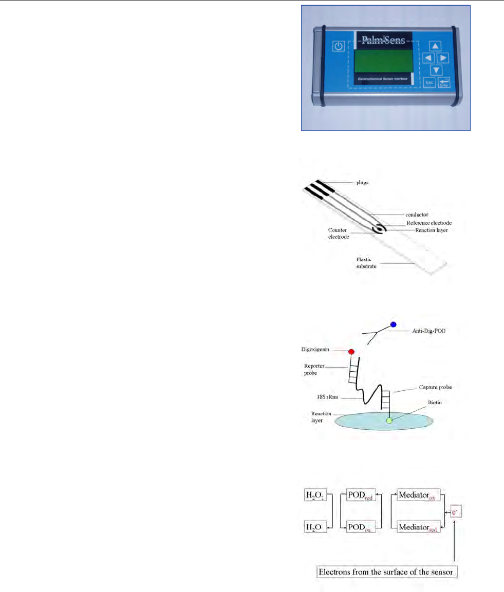
67
Microscopic and Molecular Methods for Quantitative Phytoplankton Analysis
Chapter 10 Electrochemical detection of toxic algae with a biosensor
Introduction
DNA-biosensors (devices that use molecular probes to detect
target nucleic acids in a sample) are utilised in a number of
different scientific fields. Glucose detection was one of the
first applications developed using biosensors (Clark 1956).
Electrochemical biosensors combine a biochemical recogni-
tion with signal transduction for the detection of specific mol-
ecules. The detection component such as a probe sequence,
an antibody, an enzyme or other biomolecule, catalyzes a re-
action with, or specifically binds to, the target of interest. A
transducer component then transforms this detection event
into a measurable signal. Different types of biosensors can use
optical, bioluminescent, thermal, mass and electrochemical
recognition (Gau et al. 2005). Currently, biosensors are used
in many different applications, such as the identification of in-
fectious organisms, hazardous chemicals and the monitoring
of metabolites in environmental samples (Hartley & Baeum-
ner 2003). Biosensors can be produced very cheaply for mass
production. A new detection method for the identification of
harmful algae is currently being developed using a hand held
device and biosensors (Fig. 1 and 2). The first prototype was
used to identify the toxic dinoflagellate Alexandrium ostenfel-
dii (Metfies et al. 2005). The second prototype, manufactured
by Palm Instruments BV (Houten, Netherlands) (Fig. 1), has
been extensively used to improve the biosensors. The hand
held device “PalmSens” is a compact portable potentiostat for
all kinds of electrochemical sensors and cells. It was designed
for applications in the field as well as laboratories. It can be
configured for a single application but can also be used as a
generic electrochemical instrument.
Basic principles of electrochemical de-
tection of toxic algae with a biosensor
Molecular probes
Identification of toxic algae is based on oligonucleotide probes
that specifically target ribosomal RNA. Targets for the probes
are the small and large subunit rRNA genes in the ribosomes
of the cells. The conserved and variable regions in these genes
make it possible to develop probes specific for different taxo-
nomic levels (Groben et al. 2004). The ARB (latin, “arbor”
= tree) software package can be used for probe development
(Ludwig et al. 2004). Theoretical probe specificity is depend-
ent on the number of sequences of the targeted gene available
in the databases. If molecular probes are designed from only
a few sequences, there is a danger of cross hybridisation to
non target species and organisms whose sequences are not in
the GENBANK database. Prior to the analysis of field sam-
ples, molecular probes have to be tested for specificity with
cultivated target species as well as closely related species as in
silico (calculated by means of a computer simulation) and in
situ results can show different specificity signals. Nucleic acid
probes have been developed for toxic micro-algal taxa includ-
10 Electrochemical detection of toxic algae with a biosensor
Sonja Diercks
1
*, Katja Metfies
1
and Linda Medlin
2
1
Alfred Wegener Institute for Polar and Marine Research, Am Handelshafen 12, D-27570 Bremerhaven , Germany
2
Observatoire Océanologique de Banyuls-sur-Mer, Laboratoire Arago, 66651 Banyuls-sur-Mer, France
*Author for correspondence: E-mail: sonja.dierc[email protected]
Figure 2. Sensorchip of original prototype with counter and refe-
rence electrode and the reaction layer.
Figure 1. PalmSens device from Palm Instruments.
Figure 4. Principle of redox-reaction presenting the electron trans-
port from the surface of the sensor.
Figure 3. Principle of Sandwich Hybridisation with capture and
signal probe.

IOC Manuals & Guides no 55
Chapter 10 Electrochemical detection of toxic algae with a biosensor
68
Scope
The hand held device can be used for the rapid detection of
phytoplankton in water samples. The device is a prototype and
has been further automated in an EU-funded project (Project
ALGADEC).
Detection range
The detection limit has to be determined for each probe set.
The calculated detection limit with the hand held device for
Alexandrium ostenfeldii is ~ 800 cells.
Advantages
Several probe sets have already been developed for this met-
hod.
Drawbacks
At the time of publication of this Manual, the hand held device
is still a prototype and not available for general purchase. Probes
for only a limited number of phytoplankton exist. Probes must
be validated for each region where they are applied. Genera-
tion of calibration curves are required for each probe set. High
sample volume is required if the cell densities are expected to
be relatively low. Manual RNA isolation should be done by a
trained molecular scientist. The isolation of a sufficient amount
of target rRNA from the sample to be tested is required for
this assay. A validation of probe signals against total rRNA and
over the growth cycle of the algae under different environme-
ntal conditions has to be carried out before the method can be
applied to field samples.
Type of training needed
Instruction in setting up this technique should come from a
person with an in-depth knowledge and experience of mole-
cular biology.
a) perform task: approximately five days are necessary to train
an individual in this method.
b) troubleshoot and quality control: a skilled molecular biolo-
gist should be available to solve any problems that may arise
using this method.
Essential Equipment
Incubator
Thermoheater
Vacuumpump
Washbottle
Mini-Centrifuge
Beadbeater
RNeasy Mini Plant Kit (QIAGEN)
Nanodrop Spectrophotometer
Handheld Device
Equipment cost*
€27350, $38400, for details see Table 4
Consumables, cost per sample**
0.24 € , $0.35 not including probes
Processing time per sample before analysis
Concentration of cells by centrifugation ~20 minutes, coating
of electrodes ~ 2 hours and RNA isolation ~1 hour.
Analysis time per sample
Analysis time per sample: Sandwich hybridisation ~ 2 hours.
Sample throughput per person per day
12 to 16 samples per day
No. of samples processed in parallel
Six to eight
Health and Safety issues
Relevant health and safety procedures must be followed. Read
Material Data Safety Sheets for all chemicals.
The following three chemicals are particularly hazardous
• Hydrogen peroxide 30 % (H
2
O
2
)
• N-Phenyl-1,4-benzenediamine hydrochloride (ADPA)
• β-Mercaptoethanol
*service contracts not included
**salaries not included
The fundamentals of
Electrochemical detection of toxic algae with a biosensor
69
Microscopic and Molecular Methods for Quantitative Phytoplankton Analysis
Chapter 10 Electrochemical detection of toxic algae with a biosensor
ing diatoms and dinoflagellates such as Pseudo-nitzschia and
Alexandrium (Scholin et al. 1996, Simon et al. 1997, Miller &
Scholin 1998, John et al. 2003).
Disposable sensor-chip and detection principle
The disposable biosensor chip is composed of a carrier mate-
rial on which a working electrode is printed and the detection
reaction takes place, a reference electrode and an auxiliary
electrode (Fig. 2).
The working electrode has a diameter of 1 mm and is made
of a carbon paste. A biotinylated probe is immobilised on the
reaction layer of the working electrode via avidin. The nucleic
acids are detected on the sensor chip via a sandwich-hybrid-
isation (Zammatteo et al. 1995, Rautio et al. 2003) (Fig. 3).
The underlying principle of the sandwich hybridisation is
that the target specific probe (capture probe) is immobilised
via avidin on the surface of the working electrode. If a target
nucleic acid is bound to the immobilised probe on the work-
ing electrode, the detection of the nucleic acid takes place
via a hybridisation reaction to a second target specific probe,
the signal probe that is coupled to digoxigenin (Metfies et al.
2005).
The digoxigenin specific antibody coupled to horseradish-
peroxidase is added to the sensor chip. Horseradish-peroxi-
dase catalyses the reduction of hydrogen peroxide to water.
Reduced peroxidase is regenerated by p-aminodiphenylamine
(ADPA), which functions as a mediator. The oxidised me-
diator is reduced at the working electrode with a potential
of -150 mV (versus Ag/AgCl) taking an electron from the
surface of the sensor (Fig. 4). A potential is applied between
the working and the reference electrode. The hand held de-
vice measures the resulting current activated through the flow
of the electrons from the surface. An electrochemical signal
can only be measured if the target nucleic acid binds to both
the capture and signal probes (Metfies et al. 2005). For each
target species the RNA concentration per cell has to be deter-
mined. A calibration curve must be developed for each new
probe set in order to determine the signal intensity at different
RNA concentrations. Using the information on the curve, the
electrical measurement of the hand held device can be related
to cell numbers in a field sample.
Materials
Laboratory facilities
Fume hood for RNA isolation
Equipment, Chemicals and Consumables
Information on the equipment, chemicals and consumables
used in this method are presented in the Appendix, Tables
1-2, at the end of this chapter (Tables 1-2). Suppliers, Cata-
logue numbers and estimated cost in Euros and US Dollars
are also listed in Tables 1-2.
Required Equipment (essential)
• Centrifuge
• Filter, 0.5 µm, ISOPORE™, membrane filters, Milli-
pore, Ireland
• Frit, flask and funnel, Millipore, Ireland
• Mini-Beadbeater™, Biospec products, Biospec products
Inc, USA
• Mini-Centrifuge
• Thermoshaker
• Incubator
• Vacuum pump with wash bottle
• Biosensors, Gwent Electronic Materials, Pontypool, UK
• Freezer -80 ºC
Solutions for preservation of microalgal cells
RNAlater, Ambion, Huntingdon, UK
Method
Concentration of cells
Harvesting of cells can be performed by either centrifugation
and the supernatant discarded or filtration using a filtration
device and a hand held vacuum pump (Fig. 5). A maximum
of ~ 1 x 10
7
cells can be processed with the RNeasy Plant
Mini Kit.
Preservation and storage
After collecting water samples, the algae cells can be stored at
room temperature for several days using RNALater from Am-
bion, Huntingdon, UK for a later RNA isolation. Follow the
instructions that come with RNALater carefully. The cells can
also be frozen for long term storage by flash-freezing in liquid
nitrogen and immediately transferred to -70
º
C.
RNA Isolation with the RNeasy Plant Mini Kit
(QIAGEN) (modified protocol)
General handling of RNA: Ribonucleases (RNases) are very
stable, active enzymes and are difficult to inactivate; even
minute amounts are sufficient to destroy RNA. All glassware
must first be cleaned with a detergent, thoroughly rinsed, and
oven baked at 240 ºC for four or more hours before use to
avoid any RNase contamination. Gloves must always be worn
while handling reagents and RNA samples to prevent con-
tamination from the surface of the skin or from dusty labora-
tory equipment. Isolated RNA should be stored on ice while
being processed.
RNA-Isolation
1 Add 450 µL buffer RLT with ß-ME (ß-Mercaptoethanol)
to the cells;
2 Pipette the lysate onto the glass beads and disrupt the
lysate in a bead beater for 2x 20 seconds;
3 Pipette the lysate directly onto a QIAshredder spin co-
lumn (lilac) placed in a 2 mL collection tube, and centri-
fuge for 15 minutes at maximum speed. Carefully trans-
fer the supernatant of the flow-through fraction to a new
microcentrifuge tube without disturbing the cell debris
pellet in the collection tube. Use only this supernatant in
subsequent steps;
4 Add 0.5 volume (usually 225 µL) ethanol (96–100 %) to
the cleared lysate and mix immediately by pipetting. Do
not centrifuge. Continue without delay;
5 Apply sample (usually 650 µL), including any precipi-
tate that may have formed, into an RNeasy mini column
(pink) placed in a 2 mL collection tube. Close the tube
gently and centrifuge for 15 seconds at 8000 x g. Discard
the flow-through. Reuse the collection tube in the next
step;
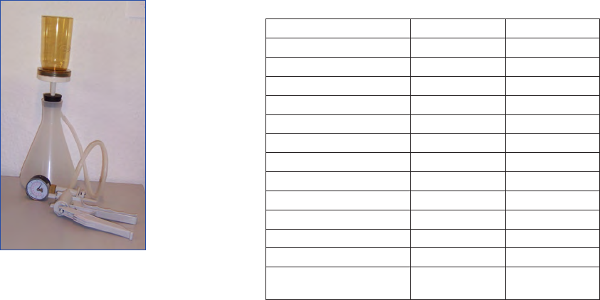
IOC Manuals & Guides no 55
Chapter 10 Electrochemical detection of toxic algae with a biosensor
70
6. Add 700 µL buffer RW1 to the RNeasy column. Close
the tube gently and wait for ca. 45 seconds, then centri-
fuge for 15 seconds at ≥8000 x g to wash the column.
Discard the flow-through and collection tube;
7 Repeat step 6;
8 Transfer the RNeasy column into a new 2 mL collection
tube (supplied). Pipette 500 µL buffer RPE onto the
RNeasy column. Close the tube gently, and centrifuge
for 15 seconds at 8000 x g to wash the column. Discard
the flow-through. Reuse the collection tube in step 9.
9 Repeat step 8;
10 Add another 500 µL buffer RPE to the RNeasy column.
Close the tube gently and centrifuge for 2 minutes at
8000 x g to dry the RNeasy silica-gel membrane;
11 To elute DNA, transfer the RNeasy column to a new 1.5
mL collection tube. Pipette 30-50 µL RNase-free water
directly onto the RNeasy silica-gel membrane. Close the
tube gently and centrifuge for 1 minute at 8000 x g to
elute;
12 To obtain a higher total RNA concentration, a second
elution step may be performed by using the first eluate
(from step 11);
13 Measure the RNA concentration by using a spectropho-
tometer e.g. Nanodrop spectrophotometer.
The isolated RNA should be flash-frozen in liquid nitrogen
and immediately transferred to -70 ºC.
Sandwich Hybridisation
A. Coating of Sensor chips
1 The sensor chips are moistened with 50 µL of carbonate
buffer (pH 9.6) (Table 1, Fig. 6), which is aspirated off
with a vacuum pump (Figs. 7-8);
2 Incubate over night in a moisture chamber at 4 ºC with 2
µL NeutrAvidin in carbonate buffer (500 µg mL
-1
) (Table
3). Store the electrodes during this period in Petri dishes
with moist Whatman filters to protect the solutions from
evaporation (Fig. 9);
3 Remove excess NeutrAvidin by washing the chips in PBS
(pH 7.6) (Fig. 10, Table 1). Then dry the chips using a
vacuum pump attached to a wash bottle;
4 Block the sensors for one hour at room temperature with
20 µL 3 % casein in PBS. Remove the casein by washing
with PBS;
Buffer Compound Concentration
Carbonate buffer (pH 9.6) NaHCO
3
50 mM
10x PBS (pH 7.6) NaH
2
PO
4
* H
2
O 0.5 M
NaCl (pH 7.6) 1.54 M
“bead buffer” NaCl 0.3 M
Tris (pH 7.6) 0.1 M
4x hybridisation buffer NaCl 0.3 M
Tris (pH 8.0) 80 mM
SDS 0.04%
10x POP buffer (pH 6.45) NaH
2
PO
4
* H
2
O 0.5 M
NaCl (pH 6.45) 1 M
PBS-BT (pH 7.6) PBS 1x
BSA 0.1 % [w/v]
TWEEN 20 (pH
7.6) 0.05 % [v/v]
5 The NeutrAvidin coated electrodes can be stored in a
fridge for at least 1 year after incubation with 2 % Treha-
lose in PBS (pH 7.6). The electrodes are coated with 15
µL of Trehalose solution and dried at 37 ºC in an incuba-
tor. Before use the electrodes should be washed with PBS
(pH 7.6) to remove the Trehalose;
B. Immobilisation of biotinylated DNA-probe
6 Coat the sensor chips with 2 µL of the biotinylated probe
[10 pmol µL
-1
in bead buffer (0.3 M NaCl, 0.1 M Tris)]
(Table 1) and incubate for 30 minutes at room temperature;
7 Add 50 µL of 1X hybridisation buffer (0.3 M NaCl, 80
mM Tris, 0.04 % SDS) onto the sensors and directly as-
pirate off to remove excess unbound probe;
8 The coated electrodes can be stored in a fridge for at least
1 year after incubation with 2 % Trehalose on PBS (pH
7.6). The electrodes are coated with 15 µL of Trehalose
solution and dried at 37 ºC in an incubator. Prior to use
the electrodes should be washed with PBS (pH 7.6) to
remove the Trehalose;
C. Sandwich Hybridisation of immobilized DNA probe, RNA
and dioxigenin labelled DNA probe
9 Fragment the RNA by using a fragmentation buffer (200
mM Tris-Acetate, pH 8.1, 500 mM KOAc, 150 mM
MgOA). Add 10 µL of rRNA to 2.5 µL fragmentation
buffer, heat for 5 minutes at 94 ºC in a thermoshaker
(Fig. 11) and immediately chill on ice;
10 Hybridisation preparation details are presented in Table
2. The positive control ensures that the probes are wor-
king and the negative control shows the detection of the
used compounds that do not contain any target RNA;
11 Heat the preparation for 4 minutes at 94 ºC in a ther-
moshaker to denature the RNA target strands. Immedia-
tely chill on ice:
12 Apply 2 µL of the hybridisation solution onto each sen-
sor. Note that each sample is applied in triplicate;
13 Incubate the chips for 30 minutes at 46 ºC in an incu-
bator then cool the incubator down to room temperature
for 5 minutes;
Figure 5. Filtration equipment and hand pump.
Table 1. Buffers for sandwich hybridisation on carbon electrodes.
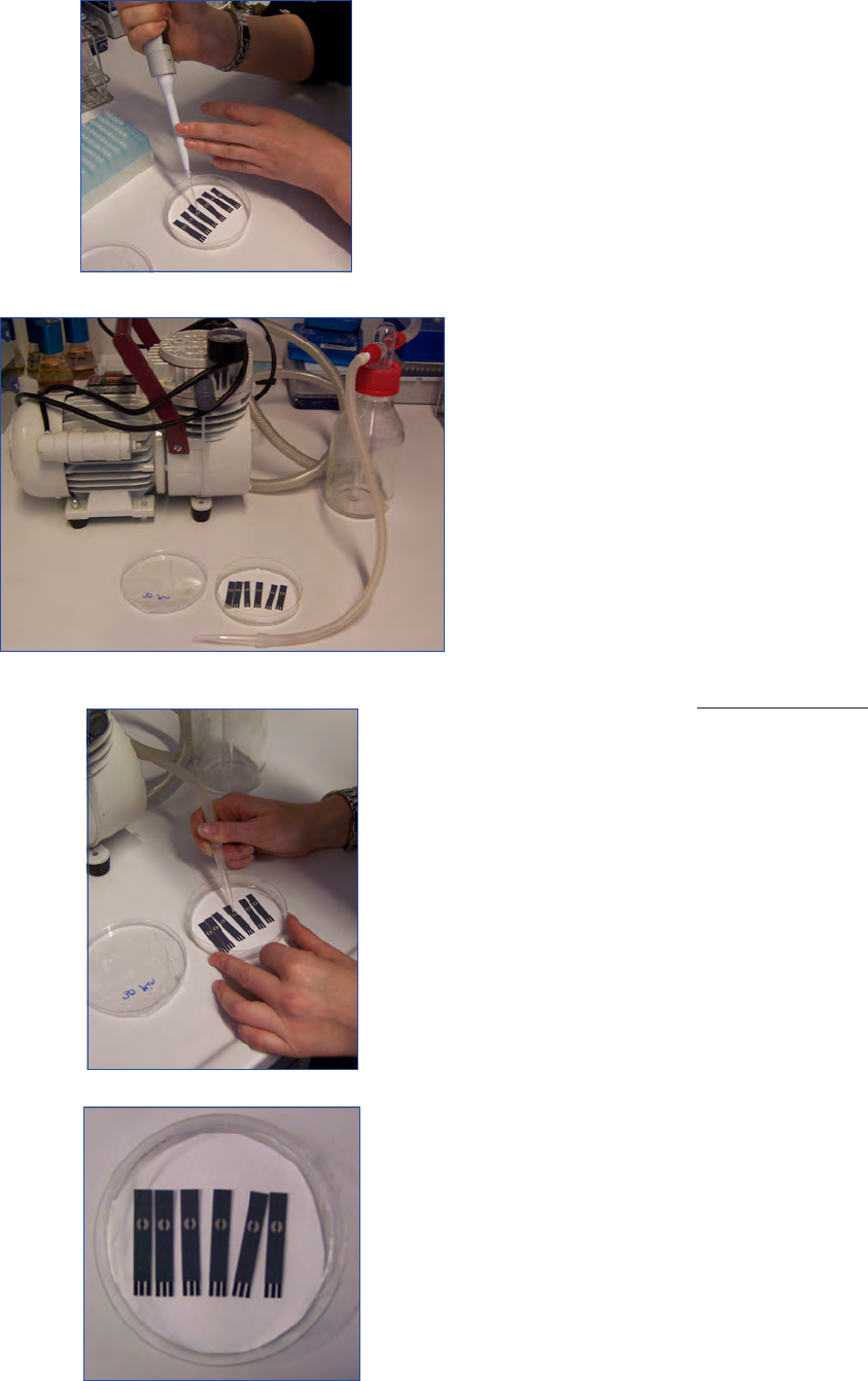
71
Microscopic and Molecular Methods for Quantitative Phytoplankton Analysis
Chapter 10 Electrochemical detection of toxic algae with a biosensor
D. Detection
14 Wash the sensors in 1X POP buffer (pH 6.45) (Table 1)
to remove excess RNA;
15 Incubate the sensors with 1.5 µL Anti-Dig-POD [7.5
U mL
-1
in PBS-BT] at room temperature for 30 minutes
(Table 1);
16 Wash the sensors separately in 1x POP buffer to remove
excess Anti-Dig-POD and dry with a vacuum pump.
17 Add 20 µL of POD substrate onto the electrode (POD
substrate contains 1.1 mg N-Phenyl 1,4-phenylenedia-
mine hydrochloride (ADPA) dissolved in 110 µL etha-
nol, 250 µL of 100 mM H
2
O
2
are added and filled up to
25 mL with 1X POP buffer);
18 Plug the chip into the hand held device and record the
measurement (Fig. 12). A summary of the buffers used
during the sandwich hybridisation process are presented
in Table 1.
Formulas for calculating results
A calibration has to be determined for each probe set to find
the signal intensity (nA) for 1 ng RNA. For each target spe-
cies, the RNA concentration per cell has to be investigated.
Subsequently the cell concentration of the target species in a
water sample can be calculated from the electrochemical sig-
nals:
Let then
Quality control
When developing this method it is useful to confirm the re-
sult signals and calculated cell counts with real cell count re-
sults. This QC system will also determine if the user training
provided is sufficient. A molecular biologist should be able to
solve any problems that arise during the experiments. False
negative signals can result for a number of reasons such as
degradation of antibodies or buffers.
Discussion
The electrochemical detection method with the hand held
device and biosensors is a rapid method to detect target algae
in a water sample. Electrodes can be mass produced. Proto-
cols and electrochemical readings of the hand held device are
simple and easy to use, read and interpret. This is useful for
people with limited experience with the method.
The hand held device has a standard operating procedure
(SOP) with many manual steps. This has now been refined
with many improvements resulting from the EU-project AL-
GADEC. Today, most of the steps are automated (an auto-
mated flow and heating chamber for the biosensors) which
now allows the detection of 14 species in parallel. The initial
sampling, filtering and RNA extraction steps remain the same.
The present biosensor consists of a disposable sensor chip
with 16 electrodes (Diercks et al. 2008a). The redox reaction
takes place between the substrate probe and the signal probe
to yield a flow of electrons. This allows for a electrochemi-
Figure 8. Drying of chips using a vacuum pump and a wash bottle.
Figure 7. Pump and washbottle for exhausting of buffers from the
electrodes.
Figure 6: Applying of buffer onto the electrodes.
Figure 9. Petri dish with Whatman filter and electrodes.
cell)(per ngRNA
) signal (probenA
numberCell
sample
)
in the(present RNA ng total ) signal (probe
n
A
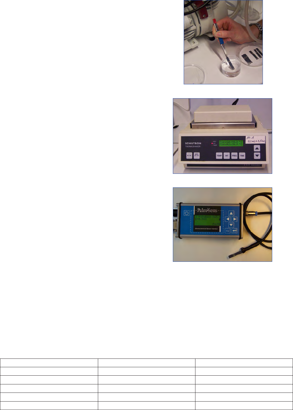
IOC Manuals & Guides no 55
Chapter 10 Electrochemical detection of toxic algae with a biosensor
72
cal detection proportional to the RNA of the target captured
on the chips and thus to the number of cells in the water
sample tested. Probes for other toxic algae (e.g., Alexandrium
minutum and Gymnodinium catenatum) have been developed
for their detection with this hand held device (Diercks et al.
2008b). About 17 different toxic algae can now be detected,
along with the negative and positive controls. These newly
developed probes are regularly reviewed for their specificity,
since new sequences are added to the available online genetic
databases daily. This cross check will help to determine if
there is any cross reactivity with other marine organisms.
The current detection limit of the hand held device can op-
erate with sample volumes of up to 8-10 Litres which is ad-
vantageous if only low cell densities of the target organism
are present in the sample. In order to isolate target RNA, an
appropriate cell density is required. The detection limit of the
hand held device for Alexandrium ostenfeldii is ~ 16.00 ng
µL
-1
, with an average yield of ~ 0.02 ng cell
-1
. This equates to
ca. 800 cells. A sampling volume of 6.4 l is required to ob-
tain a detectable amount of RNA when the target organism is
present at a cell density of 250 cells L
-1
(Metfies et al. 2005).
The manual isolation of RNA is currently the limiting fac-
tor of the system. This is because a certain quantity of high
quality RNA is required for the assay. It has been found that
separate users can isolate different qualities of rRNA from the
same sample with an equal number of algae cells present. The
resulting signal intensities cannot be compared to cell counts
determined using another enumeration technique. Genera-Genera-
tion of calibration curves is required for each probe set. A
validation of probe signals against total rRNA over the growth
cycle of the target microalgae under different environmen-
tal conditions has to be conducted to verify the calibration
curves. This will allow the extrapolation of the electrochemi-
cal readings into more accurate values of cells per Litre. A high
sample volume is required if the cell densities are low. The
automated RNA isolation developed under the ALGADEC
project will overcome some of these difficulties.
Acknowledgements
Sonja Diercks was supported by the EU-project ALGADEC
(COOP-CT-2004-508435-ALGADEC) of the 6th Frame-
work Program of the European Union and the Alfred Wege-
ner Institute for Polar and Marine Research.
Table 2. Hybridisation preparation.
Figure 11. Schutron Thermoshaker for the fragmentation and
denaturation of the sample.
Figure 10. Washing of chips in a petri dish with wash buffer.
Detection of the species Negative control Positive control
3.5 µL 4X Hybridasation buffer 3.5 µL 4X Hybridasation buffer 3.5 µL 4X Hybridasation buffer
7.5 µL rRNA 1 µL Herring DNA (3480 ng µL
-1
) 1 µL Herring DNA (3480 ng µL
-1
)
1 µL Herring DNA (3480 ng µL
-1
) 1 µL DIG marked DNA probe (1.4 pM µL
-1
) 1 µL Test DNA (36 bases, 1.4 pM µL
-1
)
1 µL DIG marked DNA probe (1.4 pM µL
-1
) 8.5 µL milliQ water 1 µL DIG marked DNA probe (1.4 pM µL
-1
)
1 µl milliQwater 7.5 µl milliQwater
Figure 12. Measuring of chips with Handheld device.
73
Microscopic and Molecular Methods for Quantitative Phytoplankton Analysis
Chapter 10 Electrochemical detection of toxic algae with a biosensor
References
Clark LC (1956) Monitor and control of blood and tissue oxygena-
tion. Trans. Am. Soc. Artif. Intern. Organs 2:41-48
Diercks S, Metfies K, Medlin, LK (2008a): Development and adap-
tation of a multiprobe biosensor for the use in a semi-automated
device for the detection of toxic algae. Biosensors & Bioelectronics
23: 1527-1533
Diercks S, Metfies K, Medlin LK (2008b) Molecular probes for the
detection of toxic algae for use in sandwich hybridization formats.
J. Plankton Res. 30, 439 - 448
Gau V, Ma S, Wang H, Tsukuda J, Kibler J, Haake DA (2005) Elec-
trochemical molecular analysis without nucleic acid amplification.
Methods 37:78-83
Groben R, John U, Eller G, Lange M, Medlin LK (2004) Using fluo-
rescently-labelled rRNA probes for hierarchical estimation of phy-
toplankton diversity – a mini-review. Nova Hedwigia 79:313-320
Hartley HA, Baeumner AJ (2003) Biosensor for the specific detec-
tion of a single viable B. anthracis spore. Anal. Bioanal. Chem
376:319-327
John U, Cembella A, Hummert C, Elbrächter M, Groben R, Medlin
LK (2003) Discrimination of the toxigenic dinoflagellates Alexan-
drium tamarense and A. ostenfeldii in co occurring natural popula-
tions from Scottish coastal waters. Eur. J. Phycol. 38:25-40
Ludwig W, Strunk O, Westram R, Richter L, Meier H, Yadhukumar,
Buchner A, Lai T, Steppi S, Jobb G, Förster W, Brettske I, Gerber
S, Ginhart AW, Gross O, Grumann S, Hermann S, Jost R, König
A, Liss T, Lüßmann R, May M, Nonhoff B, Reichel B, Strehlow
R, Stamatakis A, Stuckmann N, Vilbig A, Lenke M, Ludwig T,
Bode A, Schleifer K-H (2004) ARB: a software environment for
sequence data. Nucleic Acids Res 32:1363-1371
Metfies K, Huljic S, Lange M, Medlin LK (2005) Electrochemical
detection of the toxic dinoflagellate Alexandrium ostenfeldii with a
DNA-biosensor. Biosens. Bioelectron 20:1349-1357
Miller P, Scholin CA (1998) Identification and enumeration of cul-
tured and wild Pseudo-nitzschia (Bacillariophyceae) using species-
specific LSU rRNA-targeted fluorescent probes and filter-based
whole cell hybridization. J. Phycol 34:371-382
Rautio J, Barken KB, Lahdenpera J, Breitenstein A, Molin S, Neu-
bauer P (2003) Sandwich hybridisation assay for quantitative de-
tection of yeast RNAs in crude cell lysates. Microb. Cell Fact 2:4
Scholin CA, Buck KR, Britschgi T, Cangelosi G, Chavez FP (1996)
Identification of Pseudo-nitzschia australis (Bacillariophyceae)
using rRNA-targeted probes in whole cell and sandwich hybridi-
zation formats. Phycologia 35:190-197
Simon N, Brenner J, Edvardsen B, Medlin LK (1997) The iden-
tification of Chrysochromulina and Prymnesium species (Hyptop-
hyta, Prymnesiophyceae) using fluorescent or chemiluminescent
oligonucleotide probes: a means for improving studies on toxic
algae. Eur. J. Phycol. 32:393-401
Zammatteo N, Moris P, Alexandre I, Vaira D, Piette J, Remacle J
(1995) DNA probe hybridisation in microwells using a new bio-
luminescent system for the detection of PCR-amplified HIV-1
proviral DNA. Virol. Methods 55:185-197

IOC Manuals & Guides no 55
Chapter 10 Electrochemical detection of toxic algae with a biosensor
74
Equipment Supplier Cat. Number
€
US $
Incubator ”Shake’n’Stack” VWR 7996 2310 3189
Thermoheater ”Comfort” Eppendorf 5355R 2545 3512
Vacuumpump Omnilab 9.880540 391 539
Washbottle (250 mL) Omnilab 5051436 20 25
Mini-Centrifuge Hereaus
”Biofuge pico”
Omnilab 7025235 938 1294
Mini-Beadbeater™ Biospec products, Biospec
products Inc, USA
3110BX 715 986
Nanodrop ND1000
Spectrophotometer
Peqlap Biotechnology 91-ND-1000 8995 12418
Handheld Device Palm Instruments BV,
Houten, Netherlands
PalmSens with PC software,
Without Pocket PC
3450 4739
Sum approx. 19364 26702
Table 1. Equipment and suppliers.
Appendix

75
Microscopic and Molecular Methods for Quantitative Phytoplankton Analysis
Chapter 10 Electrochemical detection of toxic algae with a biosensor
Chemical Supplier Cat. Number
€
US $
NeutrAvidin™, biotin binding protein PIERCE, Perbio, Germany 31000 90.00 125.00
D(+)-Trehalose, ≥ 99.5 % HPLC Fluka BioChemika, Switzerland 90208 31.00 42.64
Biotin-labelled probe (18 bases) Thermo Electron
Digoxigenin-labelled probe (18 bases) Thermo Electron
Herring-Sperm DNA Roche Applied Science 10223646001 101.00 138.94
1x PBS PIERCE, Perbio, Germany 28372 83.65 115.00
Tween 20 Sigma-Aldrich Chemie GmbH, Germany P1379 26.30 36.18
N-Phenyl 1,4-phenylenediamine hydrochloride C
12
H
12
N
2
HCl (ADPA,
N-Phenyl-1,4-benzenediamine hydrochloride, 1,1-Diphenylhydrazin-
hydrochlorid) ADPA
MERCK KGaA, Germany 814648 13.10 18.00
Anti-Digoxigenin-POD fab fragments Roche Applied Science 11207733910 171.50 235.92
Hydrogen peroxide solution H
2
O
2
, 30% (w/w) Sigma-Aldrich Chemie GmbH, Germany H1009 19.40 26.69
Ethanol MERCK KGaA, Germany 100983 72.50 99.73
Sodium hydrogencarbonat NaHCO
3
Riedel-de Haën®, RdH, Laborchemikalien, GmbH
& CoKG, Germany
15.80 21.74
NaH
2
PO
4
* H
2
O MERCK KGaA, Germany 567545 29.75 40.92
NaCl Sigma-Aldrich Chemie GmbH, Germany S9888 24.80 34.11
Casein Sigma-Aldrich Chemie GmbH, Germany C5890 38.00 52.28
Tris (pH 8.0) Sigma-Aldrich Chemie GmbH, Germany T1503 101.50 139.63
SDS Sigma-Aldrich Chemie GmbH, Germany L4390 18.40 25.40
BSA Sigma-Aldrich Chemie GmbH, Germany 128910 11.40 15.74
-Mercaptoethanol MERCK KGaA, Germany 444203 60.00 82.83
RNeasy Plant Mini Kit Qiagen, Hilden Germany 74904 268.00 370.00
Whatman Chromatography Paper Whatman, Brentford, United Kingdom 3MM CHR 199.00 274.35
Glass beads (212 – 300 µm, 425 – 600 µm) Sigma-Aldrich Chemie GmbH, Germany G1277 99.00 136.19
Table 2. Chemicals and suppliers.
IOC Manuals & Guides no 55
76

77
Microscopic and Molecular Methods for Quantitative Phytoplankton Analysis
Chapter 11 Hybridisation and microarray fluorescent detection
Introduction
The introduction of DNA microarray technology in 1995 was
one of the latest and most powerful innovations in the field
of microbiology. This technique allows the rapid acquisition
of copious data (Schena et al. 1995). It is a new experimen-
tal approach in molecular biology (Blohm and Guiseppi-Elie
2001), which offers the possibility to analyse a large number
of samples using a range of different probes in parallel under a
diverse spectrum of applications (Ye et al. 2001).
Microarray technology was launched with a publication by
Schena et al. (1995). Many functional genomic methods
profit from microarrays, such as genome expression profiling,
single nucleotide polymorphism detection and DNA rese-
quencing (Lipshutz et al. 1999, Kauppinen et al. 2003, Ji and
Tan 2004, Yap et al. 2004, Al-Shahrour et al. 2005, Broet et
al. 2006, Gamberoni et al. 2006). Thus, DNA microarrays
are a powerful and innovative tool that can facilitate monitor-
ing in the marine environment.
A microarray consists of DNA sequences that are applied to
the surface of a glass slide with special surface properties in
an ordered array. It is based on a minimised form of a dot-
blot (Gentry et al. 2006, Ye et al. 2001). A DNA microarray
experiment involves microarray production, sample isolation
and preparation, hybridisation and data analysis. Prior to the
hybridisation, the target nucleic acid is labelled with a fluo-
rescent dye, which can be incorporated directly to the nucleic
acid or via indirect labelling of other substances (Cheung et
al. 1999, Southern et al. 1999, Metfies et al. 2006). The hy-
bridization pattern is captured via fluorescent excitation in a
special device, the microarray scanner (Ye et al. 2001).
The application of DNA microarrays for the identification of
marine organisms is a relatively new and innovative field of
research. It provides the possibility to analyse a large number
of targets (species or other taxa) in one experiment (Ye et al.
2001), but is not yet widely applied to marine biodiversity
and ecosystem science. For the use of microarray technology
as a standard tool with rapid and simple routine handling,
further research into methodical optimisations is required
(Peplies et al. 2003).
A number of European research groups utilise DNA micro-
arrays for the identification of marine organisms. The DNA
microarrays, or the so called “phylochip”, have been used to
identify phytoplankton (Metfies and Medlin 2004, Ki and
Han 2006, Medlin et al. 2006, Gescher et al. 2007), bacte-
ria (Loy et al. 2002, Peplies et al. 2003, Peplies et al. 2004a,
Peplies et al. 2004b, Lehner et al. 2005, Loy et al. 2005, Pe-
plies et al. 2006) and fish (Kappel et al. 2003). Specific probes
11 Hybridisation and microarray fluorescent
detection of phytoplankton
Christine Gescher*
1
, Katja Metfies
1
and Linda K. Medlin
2
1
Alfred Wegener Institute for Polar and Marine Research, Am Handelshafen 12, D-27570 Bremerhaven , Germany
2
Observatoire Océanologique de Banyuls-sur-Mer, Laboratoire Arago, 66651 Banyuls-sur-Mer, France
*Author for correspondence e-mail: Christine.Gescher@web.de
initially developed for other hybridisation assays (e.g. whole
cell) have been successfully modified and employed by the
microarray detection method.
Basic principles of hybridisation, micro-
array fluorescent detection
Hybridisation refers to the reannealing of two single strands
of nucleic acids that contain complementary sequences. It uti-
lises the basic physical structural property of DNA. DNA has
the structure of a double helix with hydrogen bonds binding
the two strands of DNA together. When the DNA is heat-
ed at a temperature above 90°C, the hydrogen bonds break
and the DNA is subdivided in two separate complementary
strands. When the temperature is decreased, the two sepa-
rate strains will reanneal. Complementary nucleic acids with
a high degree of similarity anneal easier and will bind together
more firmly. The probes on the DNA microarray represent
one strand of the DNA and if there are complementary se-
quences in the examined sample, both stands will hybridise
together. This event can be detected by a fluorescence label on
one of the two strands that have bound together.
The microarray experiment can be accomplished with ribos-
omal RNA (rRNA) or DNA, e.g. DNA-fragments generated
by a Polymerase Chain Reaction (PCR) from genomic DNA.
When using this technique to identify microorganisms rRNA
is advantageous over DNA because the cell contains rRNA in
a high number that can be easily extracted using commercial
kits. In contrast, if the number of copies of ribosomal genes in
the genomic DNA is too low then a PCR is needed to amplify
the target sequences.
The utilisation of PCR-fragments can introduce a bias to
the analyses and it has been shown frequently that microbial
communities may not be reflected correctly (Suzuki and Gio-
vannoni 1996, Wintzingerode et al. 1997, Simon et al. 2000,
Speksnijder et al. 2001, Kanagawa 2003, Medlin et al. 2006).
The hybridisation of RNA theoretically offers the possibility
of quantification and delivers a less biased view of true com-
munity composition (Peplies et al. 2006). Possible disadvan-
tages are low yields of RNA from environmental samples and
inhibition of extraction by complex organic molecules (Alm
and Stahl 2000, Peplies et al. 2006). Furthermore, the RNA
content can vary over the cell cycle, especially in prokayotes
(Medlin 2003, Countway and Caron 2006).
The method requires the use of a molecular laboratory. A clean
fume hood should be available because of ß-mercaptoethanol.
DNA microarrays consist of glass microscope slides with par-
ticular surface properties (Metfies and Medlin 2005). The

IOC Manuals & Guides no 55
Chapter 11 Hybridisation and microarray fluorescent detection
78
Scope
Detection and quantification of target phytoplankton species.
At the time of publication of this Manual, this method is relati-
vely new and currently under development.
Detection range
The detection range depends strongly on the sensitivity of the
chosen probes. Calibration curves are required to correlate cell
counts with signal point intensities.
Advantages
Allows identification of target phytoplankton to the species le-
vel.
Drawbacks
At the time of publication of this Manual, this microarray is still
a prototype and not available for general purchase. Probes for
only a limited number of phytoplankton exist. Probes must be
validated for each region where they are applied. The prepara-
tion of a calibration curve is required for each probe used.
Type of training needed
Instruction in setting up this technique should come from a
person with an in-depth knowledge and experience of mole-
cular biology.
a) perform task: approximately five days are necessary to train
an individual in this method.
b) troubleshoot and quality control: a skilled molecular biolo-
gist should be available to solve any problems that may arise
using this method.
Essential equipment
A well equipped molecular biology laboratory, see Appendix,
Table 1 for details of instrumentation.
Equipment cost*
Total set-up cost = approx. €55,000 or approx. $75,000 US
See Appendix, 2 Table 1 for details.
Consumables, cost per sample**
38 € (50 US $).
Processing time per sample before analysis
A trained person can process up to 8 samples in 6 hours:
RNA Isolation = 1 hour;
Labelling of RNA= 1 hour;
Hybridisation= 4 hours.
Analysis time per sample
A trained person can analyse up to 8 samples in 1 hour.
Sample throughput per person per day
Four samples (with duplicates of each sample) or eight single
samples.
No. of samples processed in parallel
Four samples (including duplicates) or eight single samples
Health and Safety issues
Relevant health and safety procedures must be followed.
The following chemical is particularly hazardous: β-Mercaptoe-
thanol.
*service contracts not included
**salaries not included
The fundamentals of
The hybridisation, microarray fluorescent detection method
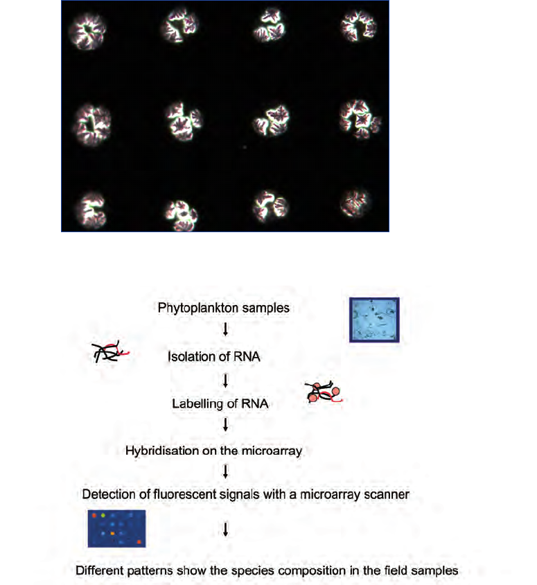
79
Microscopic and Molecular Methods for Quantitative Phytoplankton Analysis
Chapter 11 Hybridisation and microarray fluorescent detection
glass slide is coated with a special chemical surface e.g., with
aminosilane, an epoxygroup or an aldehydegroup. The probes
should be ordered with the appropriate chemical group to be
linked to the slide surface. Figure 1 shows a light microscope
picture of spots on a glass slide. Furthermore, the probes are
immobilised as spots on a glass slide in a defined pattern. Each
spot consists of many copies of an oligonucleotide probe that
is complementary to a specific target DNA sequence (Graves
1999). The target (RNAs or DNAs) hybridises to the capture
oligonucleotide probe on the microarray. The hybridisation is
detected via a fluorescent label that is attached to the target
sequence during PCR or directly to the RNA (Metfies and
Medlin 2004). The flowchart of a microarray hybridisation is
shown in Figure 2.
It may be necessary to design new probes or to choose probes
from other applications that are specific for the target taxo-
nomic group or species. If the 18S rRNA gene sequence is
used to design the probe, then it is important that the probe
be designed using only the first 1000 base pairs (bp) of the
gene.
Materials
Laboratory Facilities
This method should be carried out in a molecular laboratory
with clean fumehood facilities.
Required Equipment (essential)
Microarray production requires the following equipment:
A spotter and an oven that can be heated to 60°C. Ordered
probes can be spotted onto a glass slide using a commercial
supplier. It is more flexible and convenient to have a spot-
ter in the laboratory. However, these machines are expensive
to purchase with prices ranging from €50,000-100,000 (US
$67,000-134,000). It is advisable to outsource the spotting
procedure at the initial stage of use.
RNA isolation requires the following equipment:
• Mini-Beadbeater (e.g. BioCold Scientific Inc., USA)
used to homogenise the algal cells with glass-beads
• Conventional Mini-Centrifuge for small eppendorf tubes
(1.0 mL and 1.5 mL)
Figure 1. Microscopical view of a part of one glass slide with a grid
of 12 spots of probes diluted in 3x SSC salt buffer.
Figure 2. Flowchart of sample handling and hybridisation.
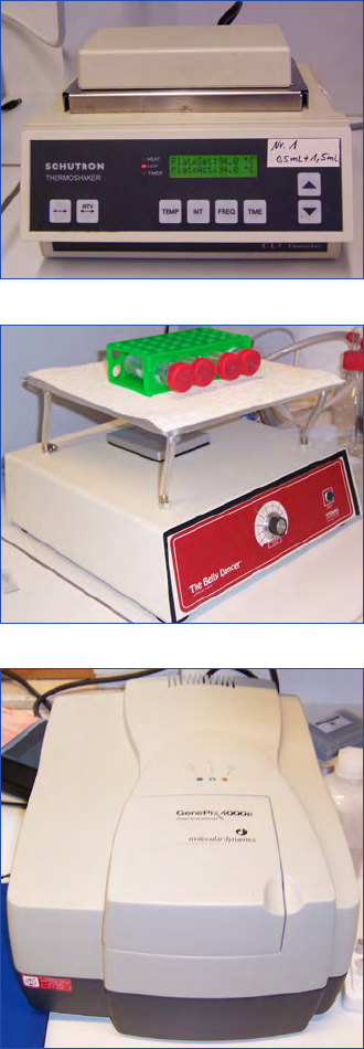
IOC Manuals & Guides no 55
Chapter 11 Hybridisation and microarray fluorescent detection
80
The hybridisation step requires the following equipment:
• Thermoheater (Fig. 3)
• Incubator
• Bellydancer or shaker (Fig. 4)
• Microarray scanner with software (Fig. 5)
Chemicals and consumables
• RNA isolation, labelling and purification:
• Isolation: RNeasy Plant Mini Kit
• Labelling of RNA: Biotin-ULS-Kit
• Purification of labelled RNA: RNeasy MinElute Cleanup
Kit
• Removal of RNAse in fume hood and labware: RNase-
Zap (Ambion Inc., Austin, USA)
Information on the equipment, chemicals and consumables
used in this method are presented in the Appendix (Tables
1-2) at the end of this chapter. Suppliers, Catalogue numbers
and estimated cost in Euros and US Dollars are also listed in
Tables 1-2.
Method
Sample Preservation and Storage
1 It is essential to begin with the correct amount of algal
material to obtain optimal RNA yield and purity with
the RNeasy columns. The required amount depends on
the target phytoplankton species and can range from 1 x
10
4
to 1 x 10
7
cells L
-1
;
2 Fresh or frozen tissue can be used. To freeze tissue for
long-term storage, the material should be flash-frozen
in liquid nitrogen and transfered immediately to -70 ºC
where it can be stored for several months. When pro-
cessing, the tissue should not be allowed to thaw during
weighing or handling prior to disruption in Buffer RLT.
Homogenised lysates, in Buffer RLT, can also be stored at
-70 ºC for several months;
3 To process frozen lysates, thaw samples and incubate for
15-20 minutes at 37 ºC in a water bath to dissolve salts;
4 It is possible to store the hybridised microarrays for at
least one year at -20 ºC, although it is usually unnecessa-
ry to keep them once they have been scanned. The reuse
of “phylochips” for new hybridisations has been tested
for expression analysis experiments where the microar-
rays were reused 5 times (Dolan et al. 2001, Bao et al.
2002);
RNA Isolation with the RNeasy Plant Mini Kit
(Qiagen)
5 Ribonucleases (RNases) are very stable and active enzy-
mes that break down RNA. They generally do not re-
quire cofactors to function. As RNases are difficult to
inactivate, even minute amounts are sufficient to destroy
RNA. Plasticware or glassware, therefore, should not be
used without first eliminating any possible trace of RNase
contamination. Care should be taken to avoid inadver-
tently introducing RNases into the RNA sample during
or after the isolation procedure. Latex or vinyl gloves
should always be worn when handling reagents and RNA
samples to prevent RNase contamination from the skin
surface or dusty laboratory equipment. Gloves should be
changed frequently and tubes kept closed whenever pos-
sible. Samples should be kept on ice, particularly isolated
RNA, especially when aliquots are being pipetted. The
use of sterile, disposable polypropylene tubes is recom-
mended throughout. These tubes are generally RNase-
free and do not require a pre-treatment to inactivate
RNases. Glassware used for RNA work should be cleaned
with a detergent, thoroughly rinsed and oven baked at
240 ºC for 4 or more hours before use;
Important notes before getting starting
6 Beta-Mercaptoethanol (ß-ME) must be added to Buffer
RLT before use. Beta-Mercaptoethanol is toxic so dis-
pense in a fume hood and wear appropriate protective
clothing. Add 10 µL ß-ME per 1 mL Buffer RLT. Buffer
RLT is stable for 1 month after the addition of ß-ME;
7 Buffer RPE is supplied as a concentrate. Before using for
the first time, add 44 mL of ethanol (96-100 %), as indi-
Figure 4. Washing of the microarrays on a belly dancer.
Figure 3. Thermoheater for denaturation of the labelled RNA.
Figure 5. Microarray scanner GenePix 4000B.
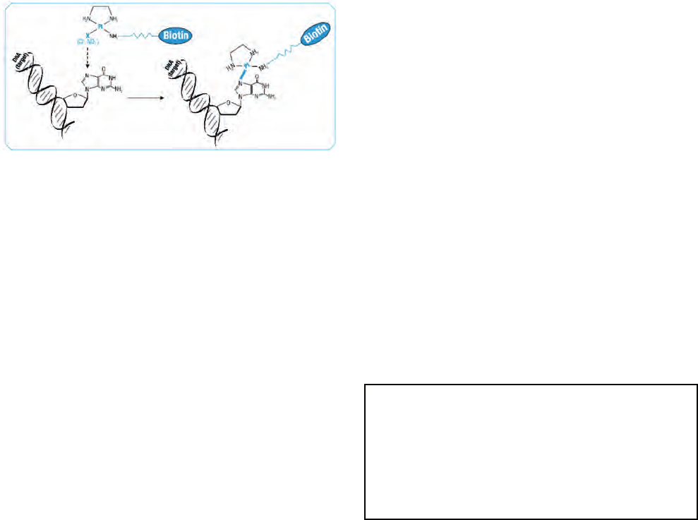
81
Microscopic and Molecular Methods for Quantitative Phytoplankton Analysis
Chapter 11 Hybridisation and microarray fluorescent detection
cated on the bottle, to obtain a working solution.
8 All steps of the RNeasy protocol should be performed
at room temperature (~20 ºC). Work quickly during the
procedure;
9 All centrifugation steps are performed at 20-25 ºC in a
standard microcentrifuge;
Harvesting of phytoplankton cells
10 Harvest the cells by centrifugation or filtration;
11 Discard the supernatant and process the cell pellet;
RNA-Isolation
12 Add 450 µL Buffer RLT with ß -ME to the cell pellet;
13 Pipette the cells into an eppendorf cup containing glass
beads (212 µm- 300 µm and 312-600 µm) and homoge-
nise the cells in a bead beater for 20 seconds;
14 Pipette the lysate directly onto a QIAshredder spin co-
lumn (lilac colour) placed in 2 mL collection tube and
centrifuge for 2 minutes at maximum speed;
15 Carefully transfer the supernatant from the flow-through
fraction to a new microcentrifuge tube without distur-
bing the cell debris pellet in the 2 mL collection tube.
This supernatant/lysate is used in all subsequent steps;
16 Add 0.5 volume (usually 225 µL) ethanol (96-100 %) to
the clear lysate, and mix immediately by pipetting. Do
not centrifuge. Continue without delay;
17 Apply the sample (usually 650 µL), including any preci-
pitate that may have formed, to an RNeasy mini column
(pink colour) placed in a 2 mL collection tube. Close the
tube gently and centrifuge for 15 seconds at ≥8000 x g
(≥10000 rpm). Discard the flow-through;
18 Reuse the collection tube in the next step;
19 Add 700 µL Buffer RW1 to the RNeasy column. Close
the tube gently and centrifuge for 15 seconds at ≥8000 x
g (≥10000 rpm) to wash the column. Discard the flow-
through and collection tube;
20 Transfer the RNeasy column into a new 2 mL collection
tube (supplied with the kit). Pipette 500 µL Buffer RPE
onto the RNeasy column. Close the tube gently and cen-
trifuge for 15 seconds at ≥8000 x g (≥10000 rpm) to
wash the column. Discard the flow-through;
21 Add another 500 µL Buffer RPE to the RNeasy column.
Close the tube gently, and centrifuge for 2 minutes at
≥8000 x g (≥10000 rpm) to dry the RNeasy silica gel
membrane;
22 To elute the RNA, transfer the RNeasy column to a new
1.5 mL collection tube. Pipette 30-50 µL RNase-free wa-
ter directly onto the RNeasy silica gel membrane. Close
the tube gently and centrifuge for 1 minute at ≥8000 x g
(≥10000 rpm) to elute;
23 To obtain a higher total RNA concentration, a second
elution step may be performed by using the first elua-
te (from the previous step). Pipette the eluate back on
the column and centrifuge for 1 minute at ≥8000 x g
(≥10000 rpm) to elute once again;
24 Measure the concentration of the RNA with a Spectrop-
hotometer (e.g. Nanodrop Spectrophotometer, Peqlab,
Erlangen, Germany).
Labelling of RNA with the Biotin-ULS-Kit
Background: This Labelling Kit uses the Universal Linkage
System (ULS) technique, which is based on the stable co-
ordinative binding of a platinum complex to nucleic acids.
The platinum complex acts as a linker between a detect-
able marker (label) molecule, i.e., fluorescein or biotin, and
DNA or RNA. The marker is coupled directly to the nucleic
acid without any significant interference. Universal Linkage
System consists of a Pt complex stabilised by a chelating di-
amine. It has two binding sites, one of which is used to bind a
marker. The other binding site is used to link the complex to
the aromatic nitrogen atoms of nucleobases and one nitrogen
atom of guanine is strongly preferred (Fig. 6). The resultant
Pt-N bond is very stable both chemically and thermally.
Features of the Biotin-ULS-Kit
• One-step reaction.
• Fast - only 30 minute to label the target.
• Universal - any nucleic acid, independent of size or
structure can be labelled.
• Easy to scale up and down. It allows labelling of as little
as 25 ng or as much as 10 µg of nucleic acid in a single
reaction
25 Add 1 µL (= ½ U) of Biotin ULS reagent to 500 ng of
nucleic acid template;
26 Adjust volume with labelling solution to 20 µL and mix
well;
27 Incubate for 30 minutes at 85 ºC;
28 Add 5 µL Stop solution and mix well;
29 Incubate for 10 minutes at room temperature;
30 Purify the solution with the RNeasy MinElute Cleanup
Kit before hybridisation;
Purification of labelled RNA with the RNeasy MinElute
Cleanup Kit (Qiagen)
31 Adjust sample to a volume of 100 µL with RNase-free
water. Add 350 µL of Buffer RLT and mix thoroughly;
32 Add 250 µL of 96-100 % ethanol to the diluted RNA
and mix thoroughly by pipetting. Do not centrifuge.
Continue the next step immediately;
33 Apply 700 µL of the sample to an RNeasy MinElute Spin
Column in a 2 mL collection tube. Close the tube gent-
ly and centrifuge for 15 seconds at ≥8000 x g (≥10000
rpm). Discard the flow-through;
34 Transfer the spin column into a new 2 mL collection
tube. Pipette 500 µL Buffer RPE onto the spin column.
Close the tube gently and centrifuge for 15 seconds at
≥8000 x g (≥10000 rpm) to wash the column. Discard
the flow-through;
35 Add 500 µL of 80 % ethanol to the RNeasy MinElute
Spin Column. Close the tube gently, and centrifuge for 2
Figure 6. Labelling of nucleic acids with Biotin-ULS (source:
www.fermentas.com)
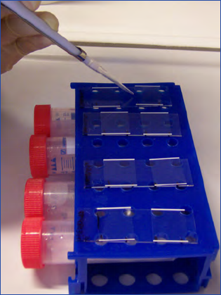
IOC Manuals & Guides no 55
Chapter 11 Hybridisation and microarray fluorescent detection
82
minutes at ≥8000 x g (≥10000 rpm) to dry the silica gel
membrane. Discard the flow through and collection tube;
36 Transfer the RNeasy MinElute Spin Column into a new
2 mL collection tube. Open the cap of the spin column
and centrifuge in a microcentrifuge at full speed for 5
minutes. Discard the flow through and collection tube;
37 To elute the RNA, transfer the spin column to a new
1.5 mL collection tube. Pipette 14 µL RNase-free water
directly onto the centre of the silica-gel membrane. Close
the tube gently and centrifuge for 1 minute at maximum
speed to elute;
38 To obtain a higher total RNA concentration, a second
elution step may be performed by using the first eluate
(from the previous step);
39 Measure the concentration of the RNA with a Spectrop-
hotometer;
Microarray Hybridisation
40 The positive control in the microarray hybridisation ex-
periment is a probe (ATGGCCGATGAGGAACGT)
specific for a 250 bp fragment of the TATA-box binding-
protein (TBP) gene of Saccharomyces cerevisiae (Metfies
and Medlin 2004);
41 The gene is amplified with the primers TBP-F (5’-ATG
GCC GAT GAG GAA CGT TTA A-3’) and TBP-R-
Biotin (5’-TTT TCA GAT CTA ACC TGC ACC C- 3’)
and is added to the hybridisation solution;
42 A negative control probe that has no match to any se-
quence found in the NCBI (National Center for Biotech-
nology Information) database should be used e.g. TCC-
CCCGGGTATGGCCGC (Metfies and Medlin 2004);
43 Pre-hybridisation step: incubate the microarrays in a mi-
croarray box containing ~ 20 mL pre-hybridisation buf-
fer [1X SET / 1 mg mL
-1
BSA] for 60 minutes at the
predetermined hybridisation temperature (58 ºC). Sub-
sequently wash the microarrays briefly in deionised water
and by centrifugation;
44 Apply 30 µL of the 40 µL hybridisation solution to the
microarray. The solution contains labelled target nucleic
acid dissolved in hybridisation buffer. The final concen-
tration of the target nucleic acid should be ~ 10 ng µL
-1
.
The solution should also contain the positive control
(i.e. 250 bp PCR-fragment TBP from S. cerevisiae with
biotin-labelled primers) in a final concentration of 4.7 ng
µL
-1
;
45 Incubate the hybridisation solution for 5 minute at 94 ºC
in a thermoheater (Fig. 3) to denature the target nucleic
acid. The use of a special kind of coverslip, the Lifter Slip
coverslip (Implen, München, Germany) is recommended
to ensure an even dispersal of the hybridisation mixture
onto the microarray;
46 Place the cover slip on the slide and pipette 30 µL of the
hybridisation mixture under the cover slip (Fig. 7);
47 Hybridise at 58 ºC for 1 hour in a wet chamber. A 50 mL
Falcon-tube with a wet Whatman paper functions very
well as a moisture chamber. Apply approximately 1 mL of
hybridisation buffer onto the Whatman paper to obtain
enough humidity in the chamber;
48 After the hybridisation is complete, remove excessive
target nucleic acid and unspecific bindings by stringent
washing of the microarrays. Remove the cover slip from
the array and put the microarray into a Falcon-tube with
50 mL wash buffer 1. Place the Falcon-tube on a belly
dancer and shake for 10 minutes (Fig. 4). Repeat this step
with wash buffer 2. Wash-buffer 1 contains: 2X SSC / 10
mM EDTA / 0.05 % SDS; wash-buffer 2: 1X SSC / 10
mM EDTA;
49 Wash again for 5 minutes with increased stringency
[wash-buffer 3: 0.2X SSC / 10 mM EDTA]. Whereas
the first washing buffer contains SDS, it is recommended
that the next 2 washing buffers do not contain SDS. This
is because residual SDS will generate high background
intensities on the microarray;
50 Remove the last wash buffer and dry the microarrays by
centrifugation in the falcon-tube (approx. 3 minutes at
approx. 2000 rpm). There are also special microarray
centrifuges with only the optimal speed;
Fluorescent Staining of the microarrays
51 Visualise the hybridised biotinylated target nucleic acids
by staining the microarray for 30 minutes at room tem-
perature in a wet chamber containing 50 µL Streptavidin-
Cy5 [0.1µg mL
-1
Streptavidin / 1X hybridisation buffer];
52 Remove excess stain by washing the microarrays twice
for 5 minutes with wash-buffer 1 and once for 5 minu-
tes with wash-buffer 2. Carry out the washing steps at
room temperature and place the microarrays in a 50 mL
Falkon-tube;
53 Dry the microarrays by centrifugation (approx. 3 minu-
tes at approx. 2000 rpm);
Analysis
54 Scan the microarray using the GenePix Axon 4000B
scanner at 635 nm;
55 Analyse the obtained signal intensities with the GenePix
6.0 software;
56 Calculate the signal to noise-ratios according to Loy et al.
(2002);
57 All calculated ratios should be normalised to the signal
of the TBP positive control. A schematic picture of the
excitation is shown in Figure 8.
Figure 7. Pipetting of hybridisation solution on one microarray.
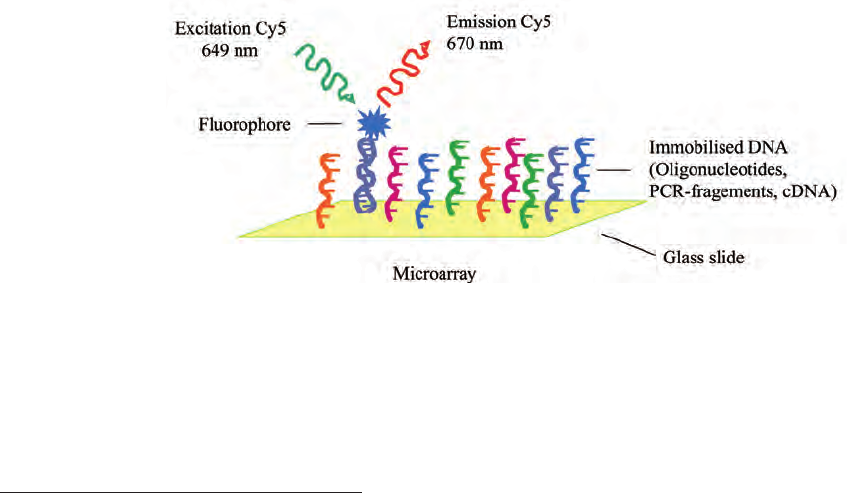
83
Microscopic and Molecular Methods for Quantitative Phytoplankton Analysis
Chapter 11 Hybridisation and microarray fluorescent detection
Formula for calculating results
Discussion
The utilisation of molecular methods has increased the po-
tential for investigating the biodiversity of phytoplankton in
the marine environment. The identification of phytoplank-
ton, especially of harmful algal species, is important from
an ecological and economic point of view. Microorganisms
dominate global biological diversity, in terms of their species
numbers, but their small size and lack of morphological fea-
tures make it difficult to assess their overall biodiversity.
In the past, regular monitoring of phytoplankton has been
hampered by the lack of reliable morphological features in
some groups of species. Even with the introduction of elec-
tron microscopy, it is difficult to make the correct classifica-
tion, especially in picoplanktonic taxa or with hidden genetic
diversity in morphological indistinguishable species (Scholin
1998, Zingone et al. 1999, Massana et al. 2002, Janson and
Hayes 2006). As a result knowledge of the complexity of the
phytoplanktonic ecosystems is still limited. Many species are
sensitive to sample fixation (Gieskes and Kraay 1983) and
some possess different life stages with varying morphological
properties (Partensky et al. 1988). The expertise of the scien-
tist may also influence the identification (Bornet et al. 2005,
Godhe et al. 2007).
The utilisation of microarrays for the detection and moni-
toring of marine microalgae, although a relatively new tech-
nique, has already undergone several trials (Metfies and Med-
lin 2004, Ki and Han 2006, Medlin et al. 2006, Gescher et
al. 2007). Previous work has shown that microarrays can be
used for the identification of phytoplankton using 18S rDNA
probes at the class level (Metfies and Medlin 2004, Medlin
et al. 2006). Ki and Han (2006) and Gescher et al. (2007)
have also demonstrated the specificity of 18S and 28S rDNA
probes for the detection of harmful algae at the species level.
One drawback of the method is the dependency on the se-
quence database for probe design. It is estimated that the
known rRNA sequence database is only a very small frac-
tion of the overall biodiversity present in the environment.
The number of 18S rRNA sequences in public databases is
constantly growing. Developed probes should be regularly
checked against all known sequences to ensure cross reactivity
with a non target organism does not occur.
The the detection limit of the microarray depends on the
sensitivity of the chosen probes. In general, a high sampling
volume of up to several Litres of seawater is required. This is
especially true if the number of cells present in the sample is
low. Another limiting factor of the microarray method lies in
the manual isolation of RNA. The manual isolation of RNA
from a set number of target cells can vary depending on the
skill of the operator. This can result in different signal intensi-
ties and so the resulting cell counts cannot be compared. The
utilisation of an automatic device (e.g. pipetting robot) for
RNA isolation may resolve this problem. The isolation of a
sufficient amount of RNA is very important because the tar-
get RNA presents only a small fraction of the RNA isolated
from a wild sample.
A calibration curve must be developed for each new probe to
monitor individual algal species. The signal must be validated
with cell numbers. A good correlation of cell counts and RNA
concentration per cell with signal intensity is prerequisite for a
reliable analysis of field samples. Different physiological con-
ditions may have an influence on the RNA content per cell.
The development and evaluation of microarrays is time-con-
suming and costly, but once a microarray is well developed,
it is a cost-effective, trusted and efficient tool to detect the
target organism. Limitations and cost aside, the use of micro-
arrays to answer ecological and biodiversity questions offers
for the first time the possibility to analyse samples with a large
number of different targets (species or other taxa) in parallel
(Ye et al. 2001). One of the most likely future uses of microar-
rays in the field of phytoplankton ecology is to monitor the
biodiversity of phytoplankton over long-time scales (Medlin
et al. 2006, Gescher et al. 2007c).
Acknowledgements
Christine Gescher was supported by the EU-project
FISH&CHIPS (GOCE-CT-2003-505491).
1000 *
)(
) (
) (
1
=
−
mLsampleofVolume
N filter whole on count cell Positive
Lcells ion concentrat Cell
1000 *
)(
) (
) (
1
=
−
mLsampleofVolume
N filter whole on count cell Positive
Lcells ion concentrat Cell
Figure 8. Microarray detection.
IOC Manuals & Guides no 55
Chapter 11 Hybridisation and microarray fluorescent detection
84
References
Al-Shahrour F, Diaz-Uriarte R, Dopazo J (2005) Discovering mo-
lecular functions significantly related to phenotypes by combining
gene expression data and biological information. Bioinformatics
21:2988-2993
Alm EW, Stahl DA (2000) Critical factors influencing the recovery
and integrity of rRNA extracted from environmental samples: use
of an optimized protocol to measure depth-related biomass dis-
tribution in freshwater sediments. J Microbiol Meth 40:153-162
Bao Z, Wenli M, Rong S, Ling L, Quiye G, Wenling Z (2002) Re-
use of a stripped cDNA microarray. Br J Biomed Sci 59:118-119
Blohm DH, Guiseppi-Elie A (2001) New developments in microar-
ray technology. Curr Opin Biotech 12:41-47
Bornet B, Antoine E, Francoise S, Marcaillou-Le Baut C (2005)
Development of sequence characterized amplified region markers
from intersimple sequence repeat fingerprints for the molecular
detection of toxic phytoplankton Alexandrium catenella (Dino-
phyceae) and Pseudo-nitzschia pseudodelicatissima (Bacillariophyc-
eae) from french coastal waters. J Phycol 41:704-711
Broet P, Kuznetsov VA, Bergh J, Liu ET, Miller LD (2006) Iden-
tifying gene expression changes in breast cancer that distinguish
early and late relapse among uncured patients. Bioinformatics 22
:1477-1485
Cheung VG, Morley M, Aguilar F, Massimi A, Kucherlapati R,
Childs G (1999) Making and reading microarrays. Nat Genet
21:15-19, (1 Suppl)
Countway PD, Caron DA (2006) Abundance and distribution of
Ostreococcus sp. in the San Pedro Channel, California, as revealed
by Quantitative PCR. Appl Environ Microbiol 72: 2496-2506
Dolan PL, Wu Y, Ista LK, Metzenberg RL, Nelson MA, Lopez GP
(2001) Robust and efficient synthetic method for forming DNA
microarrays. Nucleic Acids Res 29 :107
Gamberoni G, Storari S, Volinia S (2006) Finding biological process
modifications in cancer tissues by mining gene expression correla-
tions. BMC Bioinformatics 7:6
Gentry TJ, Wickham GS, Schadt CW, He Z, Zhou J (2006) Micro-
array applications in microbial ecology research. Microbial Ecol
52:159-175
Gescher C, Metfies K, Medlin LK (2007)
The Alex Chip - Develop-
ment of a DNA chip for identification and monitoring of Alexan-
drium. Harmful Algae, 7 (4):485 - 494
Gieskes WWC, Kraay GW (1983) Dominance of Cryptophyceae
during the phytoplankton spring bloom in the central North Sea
by HPLC analysis of pigments. Mar Biol 75:179-185
Godhe A, Cusack C, Pedersen J, Andersen P, Anderson DM, Bre-
snan E, Cembella A, Dahl E, Diercks S, Elbrächter M, Edler
L, Galluzzi L, Gescher C, Gladstone M, Karlson B, Kulis D,
LeGresley M, Lindahl O, Marin R, McDermott G, Medlin LK,
Naustvoll L-J, Penna A, Toebe K (2007) Intercalibration of clas-
sical and molecular techniques for identification of Alexandrium
fundyense (Dinophyceae) and estimation of cell densities. Harmful
Algae 6:56-72
Graves D J (1999) Powerful tools for genetic analysis come of age.
Trends Biotechnol 17:127-134
Janson S, Hayes PK (2006) Molecular taxonomy of harmful algae.
In: Granéli E, Turner JT (eds), Ecology of Harmful Algae. Eco-
logical Studies. Springer Verlag, Berlin, Heidelberg, p 9-21
Ji L, Tan K-L (2004) Mining gene expression data for positive and
negative co-regulated gene clusters. Bioinformatics 20:2711-2718
Kanagawa T (2003) Bias and artifacts in multitemplate polymerase
chain reactions (PCR). J Biosci Bioeng 96:317-323
Kappel K, Westernhagen HV, Blohm DH (2003) Microarray-based
identification of eggs and larvae from fish species common in the
North Sea. Dechema Chip-Technology Meeting, Frankfurt, Germany
Kauppinen S, Nielsen PS, Mouritzen P, Nielsen AT; Vissing H,
Moller S, Ramsing NB (2003) LNA Microarrays in Genomics.
PharmaGenomics:24-34
Ki J-S, Han M-S (2006) A low-density oligonucleotide array study
for parallel detection of harmful algal species using hybridization
of consensus PCR products of LSU rDNA D2 domain. Biosens
Bioelectron 21:1812-1821
Lehner A, Loy A, Behr T, Gaenge H, Ludwig W, Wagner M, Sch-
leifer K-H (2005) Oligonucleotide microarray for identification
of Enterococcus species. FEMS Microbiol Lett 246:133-142
Lipshutz RJ, Fodor SP, Gingeras TR, Lockhart DJ (1999) High den-
sity synthetic oligonucleotide arrays. Nature Genet 21:20-24
Loy A, Lehner A, Lee N, Adamczyk J, Meier H, Ernst J, Schleif-
er K-H, Wagner M (2002) Oligonucleotide microarray for 16S
rRNA gene-based detection of all recognized lineages of sulfate-
reducing prokaryotes in the environment. Appl Environ Micro-
biol 68:5064-5081
Loy A, Schulz C, Lucker S, Schopfer-Wendels A, Stoecker K,
Baranyi C, Lehner A, Wagner M (2005) 16S rRNA gene-based
oligonucleotide microarray for environmental monitoring of the
betaproteobacterial order ”Rhodocyclales”. Appl Environ Micro-
biol 71:1373-1386
Massana R, Guillou L, Díez B, Pedrós-Alió C (2002) Unveiling the
organisms behind novel eukaryotic ribosomal DNA sequences
from the ocean. Appl Environ Microbiol 68: 4554-4558
Medlin LK (2003) Application of molecular techniques for genetic
differentiation of microalgae. In: Norton T (ed) Out of the Past.
Dataplus, Print & Design, Belfast. p 31-48
Medlin LK, Metfies K, Mehl H, Wiltshire KH, Valentin K (2006)
Picoeukaryotic plankton diversity at the Helgoland Time Se-
ries Site as assessed by three molecular methods. Microbial Ecol
52:53-71
Metfies K, Medlin LK (2004) DNA microchips for phytoplankton:
The fluorescent wave of the future. Nova Hedwigia 79:321-327
Metfies K, Medlin LK (2005) Ribosomal RNA probes and microar-
rays: Their potential use in assessing microbial biodiversity. In:
Zimmer EA, Roalson, EH (eds) Methods in Enzymology, Mo-
lecular Evolution: Producing the Biochemical Data. Academic
Press, p 258-278
Metfies K, Töbe K, Scholin CA, Medlin LK (2006) Laboratory and
field applications of ribosomal RNA probes to aid the detection
and monitoring of harmful algae. In: Granéli E, Turner JT (eds),
Ecology of Harmful Algae. Ecological Studies. Springer Verlag,
Berlin, Heidelberg, p 311-325
Partensky F, Vaulot D, Couté A, Sournia A (1988) Morphological
and nuclear analysis of the bloom forming dinoflagellates Gyrod-
inium cf aureolum and Gymnodinium nagasakiense (Dinophyceae).
J Phycol 24: 408-415
Peplies J, Glockner FO, Amann R (2003) Optimization strate-
gies for DNA microarray-based detection of bacteria with 16S
rRNA-targeting oligonucleotide probes. Appl Environ Microbiol
69:1397-1407
Peplies J, Glockner FO, Amann R, Ludwig W (2004a) Compara-
tive sequence analysis and oligonucleotide probe design based on
23S rRNA genes of Alphaproteobacteria from North Sea bacterio-
plankton. Syst Appl Microbiol 27:573-580
Peplies J, Lau SCK, Pernthaler J, Amann R, Glockner FO (2004b)
Application and validation of DNA microarrays for the 16S rR-
NA-based analysis of marine bacterioplankton. Environ Micro-
85
Microscopic and Molecular Methods for Quantitative Phytoplankton Analysis
Chapter 11 Hybridisation and microarray fluorescent detection
biol 6:638-645
Peplies J, Lachmund C, Glockner FO, Manz W (2006) A DNA
Microarray Platform Based on Direct Detection of rRNA for
Characterization of Freshwater Sediment-Related Prokaryotic
Communities. Appl Environ Microbiol 72:4829-4838
Schena M, Shalon D, Davis RW, Brown PO (1995) Quantitative
monitoring of gene expression patterns with a complementary
DNA microarray. Science 270:467-470
Scholin CA (1998) Morphological, genetic, and biogeographic re-
lationships of the toxic dinoflagellates Alexandrium tamarense,
A. catenella and A. fundyense. In: Anderson DM, Cembella AD,
Hallegraeff GM [(eds), Physiological Ecology of Harmful Algae
Blooms. Springer Verlag, Berlin, Heidelberg, p 13-27
Simon N, Campbell L, Örnólfdóttir E, Groben R, Guillou L, Lange
M, Medlin LK (2000) Oligonucleotide probes for the identifica-
tion of three algal groups by dot-blot and fluorescent whole-cell
hybridization. J Eukaryot Microbiol 47:76-84
Southern E, Mir K, Shchepinov M (1999) Molecular interactions on
microarrays. Nat Genet 21:5-9 (1 Suppl)
Speksnijder AGCL, Kowalchuk GA, De Jong S, Kline E, Stephen
JR, Laanbroek HJ (2001) Microvariation artifacts introduced by
PCR and cloning of closely related 16S rRNA gene sequences.
Appl Environ Microbiol 67:469-472
Suzuki MT, Giovannoni SJ (1996) Bias caused by template anneal-
ing in the amplification of mixtures of 16S rRNA genes by PCR.
Appl Environ Microbiol 62::625-630
Wintzingerode FV, Goebel UB, Stackebrandt E (1997) Determina-
tion of microbial diversity in environmental samples: pitfalls of
PCR-based rRNA analysis. FEMS Microbiol Rev 21:213-229
Yap Y, Zhang X, Ling M, Wang X, Wong Y, Danchin A (2004) Clas-
sification between normal and tumor tissues based on the pair-
wise gene expression ratio. BMC Cancer 4:72
Ye RW, Wang T, Bedzyk L, Croker KM (2001) Applications of DNA
microarrays in microbial systems. J Microbiol Meth 47:257-272
Zingone A, Sarno D, Forlani G (1999) Seasonal dynamics in the
abundance of Micromonas pusilla (Prasinophyceae) and its vi-
ruses in the Gulf of Naples (Mediterranean Sea). J Plankton Res
21:2143-2159

IOC Manuals & Guides no 55
Chapter 11 Hybridisation and microarray fluorescent detection
86
Appendix
Equipment Supplier Cat. Number
€
US $
Mini-Beadbeater™ Biospec products, Biospec
products Inc, USA
3110BX 715 986
Mini-Centrifuge Hereaus
”Biofuge pico”
Omnilab, Germany 7025235 938 1294
Nanodrop ND1000
Spectrophotometer
Peqlap Biotechnology,
Germany
91-ND-1000 8995 12418
Incubator ”Shake’n’Stack” VWR, Germany 7996 2310 3189
Thermoheater ”Comfort” Eppendorf, Germany 5355R 2545 3512
Shaker (Bellydancer) Sigma Aldrich, Germany Z36, 761-3 1400 1800
Scanner and software
(GenePix 4000B device and
GenePix Pro.6.0 software)
Molecular Devices
Corporation, USA
97-0002-00 40000 51000
Sum approx.
56903 74199
Chemical Supplier Cat. Number
€
US $
Spotting (per slide) Commercial supplier or with
own spotting device
- 75 100
RNeasy Mini Plant Kit Qiagen Inc., USA 74904 268 370
Biotin-ULS Kit Fermentas Inc., USA K0631 500 640
RNeasy MinElute Cleanup Kit Qiagen Inc.,USA 742043 235 300
EDTA Sigma Aldrich, Germany E5134 80 102
Citric Acid Merck KGaA, Germany 231211 25 32
Sodium chloride NaCl Sigma Aldrich, Germany S9888 23 29
SDS Merck KGaA, Germany L4390 40 51
Bovine Serum Albumin BSA Sigma Aldrich, Germany A2153 30 38
Trizma Base Sigma Aldrich, Germany T_1503 80 102
Triton x-100 Merck KGaA, Germany 648466 33 42
Ethanol, pro Analysis Merck KGaA, Germany 1,009,832,500 73 93
1 probe (18 bases, with
Aminolink) + Positive control,
Negative control
Thermo Electron, Gemany - 100 127
Herring-Sperm DNA Roche, Germany 223646 91 116
Streptavidin-CY5 KPL, USA 079-30-00 250 319
Table 1. Equipment and suppliers.
Table 2. Chemicals and suppliers.
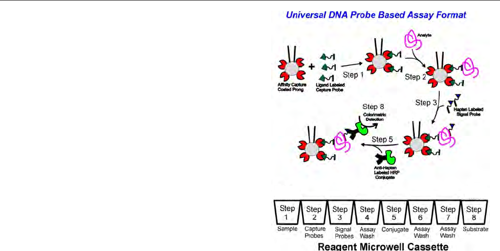
87
Microscopic and Molecular Methods for Quantitative Phytoplankton Analysis
Chapter 12 Semiautomated sandwich hybridisation
Introduction
The Sandwich Hybridisation Assay (SHA) provides a sim-
ple and rapid means to detect and estimate cell density of a
variety of algal species associated with harmful algal blooms
(HABs). Results from the SHA system can discriminate to
species level using both cultured and natural samples. Hav-
ing this level of discrimination without the need for micro-
scopy and advanced training in taxonomy, gives researchers,
public health officials and water quality managers a powerful
tool to rapidly assess changing HAB communities. The SHA
system uses species-specific, ribosomal RNA (rRNA) targeted
DNA probes that are applied using a semi-automated robotic
processor (Scholin et al. 1996, 1997, 1999, Greenfield et al.
2008). Currently, DNA probes for Pseudo-nitzschia spp., Al-
exandrium spp., Heterosigma akashiwo, Chattonella spp., and
Fibrocapsa japonica are available (Scholin et al. 2004). Others
probes include those for Coccholodinium polykrikoides (Mikul-
ski et al. 2008), a variety of Karenia spp., Karlodinium ven-
eficum and Gymnodinium aureolum (Haywood et al. 2007).
In New Zealand the SHA method has gained international
accreditation and is used to regulate shellfish harvests (e.g. Ay-
ers et al. 2005 and references therein). Recent progress made
on assays for invertebrates (Goffredi et al. 2006), including
the invasive European green crab (Jones et al. 2008), and ma-
rine bacteria (Preston, 2009) offer opportunities for use of the
SHA format to detect many other organisms as well.
Basic Principles of Sandwich Hybridisa-
tion
The SHA referred to here (after Scholin et al. 1996, 1999,
Greenfield et al. 2008) employs two DNA probes that target
ribosomal RNA (rRNA) sequences. Assays for both the large
and small subunit (LSU, SSU) rRNA have been implement-
ed. Assays are performed using pre-filled 96 well microplates
and a robotic processor supplied by Saigene Biotech Inc. A
capture probe complementary to a variable sequence is at-
tached to a mechanical solid support (prong in a sandwich
hybridisation machine), which is then submerged into the
prepared sample and hybridizes with the target molecule if
present. Captured molecules are then washed to remove any
unbound material. To detect the captured molecules, a second
hybridisation step is initiated using a DNA probe conjugated
to a signal probe. This probe is targeted to a more conserved
region of the captured fragment. The resulting “sandwich” of
capture probe/target molecule/signal probe is detected using
an enzymatically-driven colorimetric reaction. Figure 1 pro-
vides a schematic view of the sandwich hybridisation chem-
istry described above (for details see Greenfield et al. 2008).
The basic steps of the SHA method are:
1 Collect sample onto a filter,
2 Lyse sample using a chaotropic buffer (disrupts and dena-
tures the 3-D structure of macromolecules) and heat,
3 Filter lysate,
4 Load sample lysate into 96-well plate,
5 Run SHA processor (automated),
6 Record colour development (O.D. 650 and 450nm),
7 Compare results against standard curves to estimate
abundance of target species.
Laboratory Facilities
The SHA system requires a typical laboratory setting that is
protected from direct sunlight, excessive dust, and tempera-
ture extremes.
Essential Equipment
(for more details see Appendix, Table 1 at the end of this chap-
ter)
• Bench top processor (after Scholin et al. 1999)
• 96-well Microplate reader that can read wavelengths 650
nm and 450 nm
• Software to record microplate data and apply data con-
version algorithm
• Refrigerated storage (2
º
to 8
º
C)
• Vacuum filter manifold
• 85
º
C heat block
• 12-channel multiple pipette (30-300 µL)
12 Toxic algal detection using rRNA-targeted probes in a semi-
automated sandwich hybridization format
Roman Marin III* and Christopher A. Scholin
Monterey Bay Aquarium Research Institute (MBARI) 7700 Sand-holdt Rd., Moss Landing, CA 95039-0628, USA
*Author for correspondence e-mail: maro@mbari.org
Figure 1. Schematic view of the sandwich hybridisation chemistry
BACK
Well A
FRONT
Well H

IOC Manuals & Guides no 55
Chapter 12 Semiautomated sandwich hybridisation
88
Scope
Detection and quantification of a target phytoplankton species
using ribosomal RNA-targeted, DNA probe-based assays.
Detection range
Detection performance is unique to each probe set used in the
SHA system.
Advantages
The SHA system provides a robust and simple semi-automa-
ted method to detect and estimate cell abundances of target
species.
Drawbacks
Probes are only available for a limited number of target species.
Specificity of probes must be established on a regional basis.
This system may not be suitable for detection of very rare target
sequences.
Type of training needed
Instruction in setting up this technique should come from a
person with an in-depth knowledge and experience of mole-
cular biology. A minimum of three days are needed for to cover
theory, operation, data processing, etc. A skilled molecular bio-
logist should be available to solve any problems that may arise
using this method.
Essential Equipment
SHA semi-robotic processor, microplate reader, heating block,
filtration manifold, 12-channel and single channel micropipet-
tors.
Equipment cost*
SHA semi-robotic processor, €5139 (US $7500)
Total set-up cost = €14197 (US $20666).
See Appendix, Table 1 for details
Consumables, cost per sample**
€5-7 (US $7-10).
Processing time per sample before analysis
15-20 minutes (hands-on)
Analysis time per sample
75 minutes (hands-off).
Sample throughput per person per day
30-40 samples in an 8 hour day given 1 processor.
No. of samples processed in parallel
6, 8, or 12 samples with replicates 4, 3, or 2, respectively.
Health and Safety issues
Relevant health and safety procedures must be followed. The
lysis and signal probe buffers contain guanidine thiocyanate,
which can damage skin and eyes.
*service contracts not included
**salaries not included
The fundamentals of
The sandwich hybridisation method
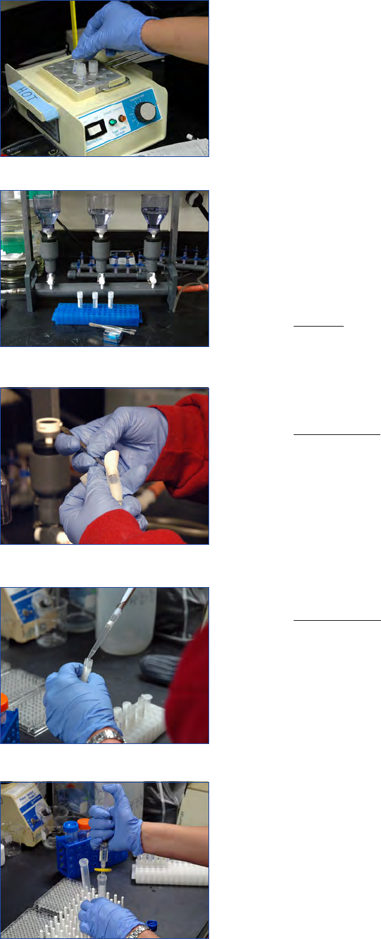
89
Microscopic and Molecular Methods for Quantitative Phytoplankton Analysis
Chapter 12 Semiautomated sandwich hybridisation
• 100-1000 µL single channel pipette
• Cold storage for samples: liquid nitrogen is preferred,
-80
o
C and –20
o
C (e.g., freezer or dry ice) can also be ef-
fective for storing archival samples (filters)
•
Chemicals and Consumables
(for more details see Appendix, Table 2 at the end of this
chapter)
• 25mm hydrophilic Durapore filter
• 2mL cryovial
• 13mm syringe filter
• 5cc syringe
• Polypropylene tubes 12X 75mm
• 10% H
2
SO
4
• filling trays/pipette tips
Probes
The suite of SHA probes currently available for HAB spp.
include the following:
Diatoms
Pseudo-nitzschia australis (and other diatoms below, Scholin
et al. 1999)
Pseudo-nitzschia multiseries
Pseudo-nitzschia pungens
Pseudo-nitzschia pseudoelicatissima/multiseries complex
Dinoflagellates
Alexandrium tamerense/catenella/fundyense (North American
ribotype, Matweyou et al. 2004, Anderson et al. 2005)
Cochlodinium polykrikoides (Mikulski et al. 2008)
Gymnodinium aureolum (and other dinoflagellates below,
Haywood et al. 2007)
Karenia brevis
Karenia mikimotoi
Karenia selliformis
Karenia papilionacae
Karlodinium veneficum
Raphidophytes
Heterosigma akashiwo (and others below, Tyrrell et al. 2001,
2002, Scholin et al. 2004)
Fibrocapsa japonica
Chattonella antiqua/subsalsa
Method
Preparation to run samples
1 Turn on heating blocks for sample lysis (Fig. 2) and pro-
cessor and check that desired temperatures are at their
proper values. Lysis is carried out at 85
º
C. The processor
plate should provide a temperature of 28-30
º
C.
2 Obtain necessary lysis tubes for runs or alternatively label
2 mL cryovials for storage of sample filters in liquid nitro-
gen for later analysis (see below).
3 Start the microplate reader.
4 If using pre-made plates, remove seal and let it reach room
temperature protected from light and dust. If required,
dispense reagents into 96-well microplate as shown in the
instruction booklet that comes with materials supplied
by Saigene Corporation (see also Greenfield et al. 2006).
When dispensing reagents to a microplate use barrier tips
Figure 2. Heating block set to 85ºC used for sample lysis.
Figure 3. Three-position vacuum filter manifold used to
collect particulate fraction of water sample.
Figure 4. Filter, sample side in, being placed in cryovial for
archival and/or lysis.
Figure 5. Addition of lysis buffer to cryovial with filter.
Figure 6. After lysis, lysate is syringe filtered into clean tube.
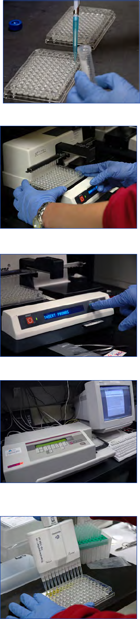
IOC Manuals & Guides no 55
Chapter 12 Semiautomated sandwich hybridisation
90
to minimise cross-well contamination. Dispense 0.25 mL
per well. Do not blow out small amounts of fluids fol-
lowing primary delivery of reagents and samples to the
plate or excessive bubbles will form in the well; bubbles
can interfere with the assay.
Sample, plate and prong handling
5 Protect plate and sample from sunlight and excessive
heat. Samples should be filtered and lysed as soon as pos-
sible, or filters can be archived for later analysis by rolling
the filter into a cryovial (particles away from the tube wall
and freezing the filters in liquid nitrogen or alternative
cold storage). Use plate within 1 hour after removing
seal and/or dispensing reagents. Prongs should remain in
package until used. Handle prongs with forceps touching
only the strip, or backbone, that connects the 12 prongs;
avoid touching the prongs themselves. Store prongs at
4-8
º
C with packaging and desiccant provided.
Sample filtration
6 Samples should be collected using a vacuum manifold
at a vacuum pressure of approximately 100-150 mmHg
(Fig. 3). Filter samples onto hydrophilic Durapore fil-
ters (generally 0.65-0.45 µm pores size; Millipore). The
volume filtered should be no more than what can pass
through the filter in about 20 minutes. Typical sample
volumes are 200 to 400 mL of whole water. Samples that
have been pre-concentrated (e.g. net tow or sieve) can
also be collected on the Durapore filter as well.
Archival and Lysis of Sample
7 After filtering, place filter membrane into a 2 mL cryo-
vial. Place the filter with the sample side facing away from
the tube wall. Do not crumple the filter and be sure to
push the filter to bottom of the tube (Fig 4). If sample is
to be archived, cap the 2 mL cryovial and store in liquid
nitrogen without lysis buffer.
8 To process, add 1-2 mL of lysis buffer to cryovial with
filter and cap it tightly (Fig 5). Place cryovial in heating
block with wells half filled with water to enhance heat
transfer (Fig. 2). Heat for 5 minutes total with a brief
finger vortex after 2.5 minutes.
9 After heating, allow lysate to cool for 5 minutes. Use ly-
sate within 20 minutes of preparation.
10 Remove plunger from a 5 cc disposable syringe (Becton
and Dickinson).
11 Install a 13 mm, 0.45 µm Millex-HV (Millipore) filter
onto the syringe.
12 Place tip into a clean polypropylene collection tube, add
lysate to syringe barrel and push lysate through filter until
foam appears at the tip of filter (Fig. 6). Lysates from re-
plicate samples may be combined to yield a larger volume
of lysate from a given sample.
13 The lysate is now ready to be loaded onto the plate sam-
ple well (row H).
Processing
14 Load 0.25 mL filtered lysate per sample well (Fig. 7).
15 Load prong onto processor arm and secure spring clip.
Do not handle prong with bare hands. Hold prong by the
backbone with tweezers and avoid scraping the prongs
against the processor arm.
Figure 7. Lysate (0.25 mL) is added to appropriate sam-
ple wells on microplate.
Figure 8. Microplate being placed on processor after
prongs added to processor arm.
Figure 9. Processor being started after plate is positio-
ned on heater base.
Figure 10. Microplate is placed on microplate reader
cradle; optical density is recorded at 650nm for row “A”
(wells in which colour development has occurred).
Figure 11. After microplate is read at 650nm, row “A” is acidified
with 50 µL of 10% H
2
SO
4
;optical density is recorded at 450 nm for
row “A”. The measure at 650 nm is considered low sensitivity while
that at 450 nm is considered high sensitivity. For positive samples,
the optical density at 450 nm should be roughly 2X that at 650 nm.

91
Microscopic and Molecular Methods for Quantitative Phytoplankton Analysis
Chapter 12 Semiautomated sandwich hybridisation
16 Mount 96 well microplate onto processor, make sure to
centre the microplate on the heating plate (Fig. 8).
17 Push the “RUN” button (Fig. 9) and make sure that the
prongs enter the wells without touching the sides of the
wells. The plate will be ready to read in just over an hour.
A digital timer will display time remaining; the counter
will read “0” approximately 90 seconds before the process
is actually complete. The processor will display a mes-
sage indicating that the reaction is complete, and plate is
ready to be read.
Reading the Plate
18 When the processor is finished, immediately read the
plate(s) (Fig. 10).
19 First read the plate at 650 nm.
20 Next acidify row A with 50 µL of 10 % H
2
SO
4
(add and
mix using a 12-channel pipette and avoid introduction of
bubbles) (Fig. 11).
21 After all bubbles have popped (~10-45 seconds) read
plate at 450 nm.
Data Processing
To calculate the concentration of target in a sample, the as-
say requires that you establish an empirically derived dose re-
sponse curve that relates optical density (O.D.) to a known
number of cells per well of lysate (see Greenfield et al. 2008,
Haywood et al. 2007, Ayers et al. 2005 for details in estab-
lishing a dose response curve). Using optical density (from
the assay), the dose response curve, sample volume and lysis
buffer volume (used to lyse the sample) you can estimate the
target abundance in the sample. Below is the equation used to
convert cells per well to cells per mL.
Here is an example of how you use the above equation to
estimate target abundance in a sample. You filter 500mL (X)
of water onto a filter and lyse this sample in 2.0 mL of lysis
buffer (Y). Using the SHA system you obtain an O.D. that
translates to 625 cells per well (from the dose response curve).
Then using the formula you estimate a target abundance of
10 cells per mL in your sample.
Controls
Positive and negative controls are available to check system
integrity and performance (e.g. Greenfield et al. 2006).
Sample Collection and Preservation
Samples should be run or archived as soon as possible after
collection. Prior to filtration, samples should be kept cool and
protected from excessive light. If the sample cannot be run
within several hours it should be filtered and stored frozen. A
sample stored in liquid nitrogen can be held for up to 1 year
or longer. Samples can also be stored in a -80
º
C freezer or on
dry ice for up to 1 week. It may be possible to store preserved
samples at room temperature as well (see Tyrrell et al. 2002).
Discussion and system considerations
The goal of SHA system is to give the research/monitoring
community a method to quickly and conveniently screen
samples for a variety of HAB species. Once samples are col-
lected, processing takes approximately 1.25 hours. No target
amplification is required so problems that can affect ampli-
fication based systems (e.g. extensive sample handling, PCR
inhibition) are avoided. The absolute detection level of the
SHA system is dependant on the designs of the capture and
signal probes. An important feature of the SHA system is that
it is relatively insensitive to biomass, so techniques such as
sieving to collect large volumes of sample can be used with-
out impacting system performance, provided proper control
experiments have been performed to verify assay results from
a given region and wide range of samples. Further increases
in sensitivity can also be achieved by lysing the sample in a
smaller volume of lysis buffer to increase target cell concentra-
tion. The SHA system is not suitable for very rare targets (e.g.
single copy genes); in those cases some kind of amplification
technique may be desirable.
All methods relying on molecular probes for detection can
be subject to cross-reaction with non-target species. Therefore
after an initial positive result, an alternative method (micro-
scopy, toxin detection, PCR, etc.) should be used to confirm
results until such time that confidence in the efficacy of probe
is known. Some probes may work well for certain species in
certain regions, but not all probes will work equally well in
different geographic regions. Moreover, species designations
as defined using traditional criteria (morphology, ultrastruc-
ture, pigments, etc.) may not agree with those based on rRNA
sequence identity (e.g. see Scholin et al. 2004, Ayers et al.
2005, Lundholm et al. 2006). Provisions should also be made
to store replicate samples in case of system failure or if results
require further analysis or reconfirmation is desired.
Use of the SHA system requires that probes be available for
the target species of interest. Currently, probes are available
for a variety of HAB spp. (see above) as well as other organ-
isms. The creation of probes for this system often requires
iterative probe design (trial and error) which can incur con-
siderable time and expense. Ideally, cultures of the targeted
species are used to create calibration curves and to spot check
the system when reagent batches are changed.
The SHA system uses chemistry that is designed to work at
30
º
C. If the ambient temperature exceeds this value, the sys-
tem will not function properly and steps to lower ambient
temperature will need to be taken. Some of the reagents used
in the SHA system are required to be refrigerated and pro-
tected from direct sunlight.
Acknowledgements
X mL sample
filter
filter Y mL lysate
lysatemL
well
well
cells
sampleinmLperCells
xx
25.0
x
500 mL sample
filter
filter 2 mL lysate
lysate mL
well
well
625 cells
xx
25 . 0
x
mL of sample
10 cells
=
IOC Manuals & Guides no 55
Chapter 12 Semiautomated sandwich hybridisation
92
Development and application of the SHA for HAB research
have been sponsored in large part by grants from the David
and Lucille Packard Foundation (allocated by the Monterey
Bay Aquarium Research Institute), the National Science
Foundation (9602576 and OCE-031422), and the National
Oceanic Atmospheric Administration Saltonstall-Kennedy
Grant Program (NOAA NA57D009) to C.A.S.
References
Anderson DM, Kulis DM, Keafer BA, Gribble KE, Marin R, Scho-
lin CA (2005) Identification and enumeration of Alexandrium
spp. from the Gulf of Maine using molecular probes. Deep-Sea
Res II 52:2467-2490
Ayers K, Rhodes L, Tyrrell J, Gladstone M, Scholin C (2005) In-
ternational accreditation of sandwich hybridisation assay for-
mat DNA probes for micro-algae. N. Z. J. Mar. Freshwater Res.
39:1225–1231
Greenfield D, Marin III R, Doucette GJ, Mikulski C, Jensen S, Ro-
man B, Alvarado N, Scholin CA. (2008) Field applications of the
second-generation Environmental Sample Processor (ESP) for
remote detection of harmful algae: 2006-2007. Limnology and
Oceanography: Methods 6: 667-679.
Greenfield DI, Marin III R, Jensen S, Massio E, Roman B, Feld-
man J, Scholin C (2006) Application of the Environmental Sam-
ple Processor (ESP) methodology for quantifying Pseudo-nitzschia
australis using ribosomal RNA-targeted probes in sandwich and
fluorescent in situ hybridisation. Limnol Oceanogr Methods
4:426-435.
Goffredi SK, Jones W, Scholin CA, Marin R, Hallam S, Vrijenhoek
RC (2006) Molecular detection of marine larvae. Marine Biotech-
nology 8: 149-160.
Haywood AJ, Scholin CA, Marin III R, Steidinger KA, Heil CA,
Ray J (2007) Molecular detection of the brevetoxin-producing
dinoflagellate Karenia brevis (Dinophyceae) and closely related
species using ribosomal RNA probes and a semi-automated sand-
wich hybridization assay. J Phycol 43:1271–1286
Jones WJ, Preston C, Marin III R, Scholin C, Vrijenhoek R (2008)
A Robotic Molecular Method for in situ Detection of Marine In-
vertebrate Larvae. Mol Ecol Resour 8:540-550
Lundholm N, Moestrup Ø, Kotaki Y, Scholin C, Miller P (2006)
Inter- and intraspecific variation of the Pseudo-nitzschia delica-
tissima-complex (Bacillariophyceae) illustrated by rRNA probes,
morphological data and phylogenetic analyses identification of P.
decipiens and P. dolorosa spp. Nov. J Phycol 42:464-481
Matweyou JA, Stockwell DA, Scholin CA, Hall S, Trainer VL, Ray
JD, Whitledge TE, Childers AR, Plumley FG (2004) Use of Alex-
andrium rRNA targeted probes to predict PSP events on Kodiak
Island, Alaska. In: Steidinger KA, Landsberg JH, Tomas CR, Var-
go GA (eds) Harmful Algae 2002. Florida Fish and Wildlife Con-
servation Commission, Florida Institute of Oceanography, and
Intergovernmental Oceanographic Commission of UNESCO, St.
Petersburg, Florida, USA., p 267-269
Mikulski CM, Park YT, Jones KL, Lee CK, Lim WA, Lee Y, Scho-
lin CA, Doucette GJ (2008) Development and field applica-
tion of rRNA-targeted probes for the detection of Cochlodinium
polykrikoides Margalef in Korean coastal waters using whole cell
and sandwich hybridization formats. Harmful Algae 7:347-359
Preston C., Marin III R, Jenson S, Feldman J, Massion E, De-
Long E, Suzuki M, Wheeler K, Cline D, Alvarado N, Scholin
C. (2009) Near real-time, autonomous detection of marine bac-
terioplankton on a coastal mooring in Monterey Bay, California,
using rRNA-targeted DNA probes. Environmental Microbiology
11:1168-1180
Scholin CA, Buck KR, Britschgi T, Cangelosi J, Chavez FP (1996)
Identification of Pseudo-nitzschia australis (Bacillariophyceae) us-
ing rRNA-targeted probes in whole cell and sandwich hybridiza-
tion formats. Phycologia 35:190 – 197
Scholin C, Miller P, Buck K, Chavez F, Harris P, Haydock P, Howard
J, Cangelosi G (1997) Detection and quantification of Pseudo-
nitzschia australis in cultured and natural populations using LSU
rRNA-targeted probes. Limnol Oceanogr 42:1265–1272
Scholin CA, Marin III R, Miller PE, Doucette GJ, Powell CL,
Haydock P, Howard J, Ray J (1999) DNA probes and a receptor-
binding assay for detection of Pseudo-nitzschia (Bacillariophyceae)
species and domoic acid activity in cultured and natural samples.
J Phycol 35:1356-1367.
Scholin CA, Vrieling E, Peperzak L, Rhodes L, Rublee P (2004) De-
tection of HAB species using lectin, antibody and DNA probes.
In: Hallegraeff GM, Anderson DM, Cembella AD (eds) Manual
on harmful marine microalgae, Vol 11. IOC, UNESCO Paris, p
131-164
Tyrrell JV, Connell LB, Scholin CA (2002) Monitoring for Heter-
osigma akashiwo using a sandwich hybridisation assay. Harmful
Algae 1:205-214
Tyrrell JV, Scholin CA, Berguist PR, Berguist PL (2001) Detection
and enumeration of Heterosigma akashiwo and Fibrocapsa japonica
(Raphidophyceae) using rRNA-targeted oligonucleotide probes.
Phycologia 40:457-467

93
Microscopic and Molecular Methods for Quantitative Phytoplankton Analysis
Chapter 12 Semiautomated sandwich hybridisation
Appendix
Table 1. Equipment and suppliers. Note that some pieces of equipment, such as the plate reader, sample filtration system, heating block
and refrigerator, are available as other models from a variety of vendors. Prices quote obtained December, 2007.
Equipment Supplier Cat. Number
€
US $
96-well Microplate reader that can
read wavelengths 650 nm and 450 nm
Fisher Scientific 14-386-27 3821 5510
Optical filter 650nm Fisher Scientific 14-386-59 196 283
Vacuum filter manifold Fisher Scientific 09-753-39A 540 779
25 mm polysulfone filter funnel
(250 mL) need 6, costs in total
Pall 4203 504 726
Vacuum pump GAST DOA P704 AA 303 443
Heating block Fisher Scientific 11-716-68Q 223 322
12-Channel Pipettor 20-300 µL Rainin L12-300 412 595
Single Channel Pipettor 10-1000 µL Rainin PR-1000 184 265
Robotic processor Saigene Inc
5
. 6000-01 5708 8500
Refrigerator (4-8
o
C) Maytag MBB1952HE 577 850
Cryogenic Storage vessel Fisher Scientific 11-676-1C 2350 3393
Sum approx. 14818 21666

IOC Manuals & Guides no 55
Chapter 12 Semiautomated sandwich hybridisation
94
Table 2. Expendable reagents and supplies required for application of the SHA and relevant suppliers.
Material Supplier Cat. Number
€
US $
1
Custom Plate One Probe
Set; minimum order of 50
plates
Saigene
5
call for order 25 38 per plate
1
Custom Plate Two Probe Set;
minimum order of 50 plates
Saigene
5
call for order 27 40
1
Custom Plate Three Probe
Set; minimum order of 50
plates
Saigene
5
call for order 28 42
1
Custom Plate Four Probe
Set; minimum order of 50
plates
Saigene
5
call for order 29 44
2
Assay Development Kit;
minimum order of 25 plates
Saigene
5
call for order 24 36
3
Bulk lysis buffer, 500 mL Saigene
5
call for order 27 40
4
Defined Kits (routine
production), incl lysis buffer,
prong, sample filters, etc.
Call for quote Call for quote
25 mm Durapore filter (100
count)
Millipore DVPP02500 60 86
13 mm syringe filter (100
count)
Millipore SLHVT13NL 138 197
Polypropylene 12X75mm
tubes (5000 count)
Fisher Scientific 14-961-11 318 459
5 cc Syringe (400 count) Fisher Scientific 14-823-35 47 68
2 mL Cryovial (250 vials) Fisher Scientific 03-337-7H 127 184
Filling boats (200 count) Fisher Scientific 07-200-127 76 110
10% H
2
SO
4
(dilute stock) Fisher Scientific A300-500 40 58
Sum approx. 966 1402
1
Plates made custom to user specification. Saigene will fill and seal plates; user supplies capture and signal pro-
bes. Plates are configured with one to four probe sets. Price includes prongs; lysis buffer sold separately. Discount
available for orders >50 plates.
2
Plates filled with all reagents except capture and signal probes (to facilitate assay development). Price includes
prong, buffers for preparing capture and signal probe solutions. Discount available for orders >25 plates.
3
In addition to lysis buffer, Saigene can provide bulk quantities of other reagents used in the SHA; prices available
on request.
4
Defined Kits are those prepared entirely by Saigene. They differ from Custom Plate configurations in that Saigene
provides user-defined probes, or those available through published articles. Defined Kits also include prongs and
lysis buffer (volume based on the intended use of the plates), and can be bundled with sample and lysate filters if
desired. The most likely application of Defined Kits are for research/monitoring programs where there is a defined
set of target species/probes, sample and lysis volumes are fixed within well specified range, and users prefer not
to take responsibility for procurement and quality assurance of probe stocks. Depending on the number of plates
ordered, Defined Kits will generally exceed those in cost of the equivalent Custom Plate by 10-20% depending on
probe costs and number of probe sets required per plate.
5
Saigene Biotech Inc.
ATTN: Thomas Hurford
Box 3048
Monument, CO 80132
USA
Phone Int.+ 1 719-559-1163

95
Microscopic and Molecular Methods for Quantitative Phytoplankton Analysis
Chapter 13 Quantitative PCR
13 Quantitative PCR for detection and enumeration of phyto-
plankton
Luca Galluzzi*
1
and Antonella Penna
2
1
Section for Biotechnology, Department of Biomolecular Sciences, University of Urbino, Via Campanella 1, 61032 Fano (PU), Italy
2
Section of Environmental Biology, Department of Biomolecular Sciences, University of Urbino, V.le Trieste 296, 61100 Pesaro (PU), Italy
*Author for correspondence e-mail: [email protected]
Introduction
Quantitative Polyemerase Chain Reaction (QPCR) is an ex-
tremely sensitive method which has been applied in recent
years to detect and quantify different phytoplankton spe-
cies in environmental samples (Bowers et al. 2000, Popels et
al. 2003, Galluzzi et al. 2004, Coyne et al. 2005, Park et al.
2007, Touzet et al. 2009). Its application could revolutionise
the study of microalgal population dynamics in marine sys-
tems as it allows the concurrent identification, enumeration
and determination of viability of target species (Coyne and
Cary 2005, Kamikawa et al. 2005). QPCR can be used on
both seawater and sediment samples. The method is based
on the amplification of specific DNA sequences. In assays
developed to date for phytoplankton these sequances consist
of ribosomal RNA (rRNA) genes. Many protocols have been
optimised for the QPCR approach. Here, we describe an op-
timised protocol, which is based on the use of SYBR Green (a
dye which specifically binds to DNA) and relies on a standard
curve constructed with a DNA plasmid containing the cloned
target sequence for quantification.
Basic Principles of Quantitative PCR
(QPCR)
Polymerase Chain Reaction is a technique used to amplify in
vitro a target sequence of DNA. The PCR is performed by
heating and cooling an initial reaction mixture in a defined
series of temperature steps. The reaction mix contains DNA
from the sample to be tested, two different primers (small
bits of artificially synthesised DNA complementary to the tar-
get DNA in which you are interested) nucleotides consisting
of the four different bases required to make DNA, a DNA
polymerase enzyme which will build DNA using the nucle-
otides and buffer containing various salts which are optimal
for the functioning of the DNA polymerase. The different
temperature steps are necessary to separate the two strands
in the double helix DNA (denaturation step), to allow the
binding of the primers to the complementary DNA present
in the sample (annealing step) and to permit DNA synthesis
by the DNA polymerase (elongation step). The specificity of
the PCR is mainly due to the primer sequences which must
be complementary only to the DNA region targeted for am-
plification. The annealing temperature is of particular impor-
tance. If too low an annealing temperature is used, then the
primers may anneal to regions of DNA which are similar but
not identical.
As the PCR progresses, the DNA generated by the reaction
is used as a template for replication leading to the exponen-
tial amplification of the target DNA sequence. A typical PCR
amplification profile consists of an exponential amplication
of the target sequence, followed by a linear or plateau phase
as reagents become exhausted as seen in Figure 1.
The qualitative analysis of the PCR reactions is performed
at the end point of the reaction. This is usually performed
by agarose gel electrophoresis and ethidium bromide staining.
This method of visualising this PCR DNA product involves
placing the PCR product in a well in a thin block of agar-
ose gel and passing an electric current, negative to positive,
through the gel. DNA is a negatively charged particle and will
migrate with the current through the gel. Because all of the
PCR products are the same size i.e. the size determined by the
distance between where the two primers originally bound to
the opposite strands of the DNA during PCR amplification,
all the PCR products will migrate at the same rate forming a
dense band of DNA. The agarose is infused with ethidium
bromide, a stain which binds to DNA. Ethidium bromide
fluoresces under UV light. When the gel is viewed under UV
light the PCR product can be easily seen as a fluorescent band
where the ethidium bromide has concentrated in the DNA.
The brightness of the PCR band is related to the amount of
PCR product present at the end of the PCR reaction (the
plateau phase).
In quantitative real-time PCR (QPCR), reactions are ana-
lysed during the initial exponential phase rather than at the
end point. PCR product formation is monitored after each
cycle in real time by measuring a fluorescence signal which
is proportional to the amount of PCR product generated.
This is performed using a camera incorporated within a real-
time PCR machine. Software converts the data recorded by
the camera and allows the visualization of the amplification
curves on a computer screen. An example of this can be seen
in Fig. 2. The fluorescence can be generated by using inter-
calating (binding between the grooves of the double helix
PCR product
Cycle number
A B
Figure 1. General PCR amplification profile. The exponential amp-
lification phase (a) is followed by a linear or plateau phase (b), due
to reactants exhaustion

IOC Manuals & Guides no 55
Chapter 13 Quantitative PCR
96
Scope
Detection and quantification of target phytoplankton species.
Detection range
Detection performance varies with the sample volume, more
precisely: 10 target sequences in a 25 µL reaction tube. The
method is sufficiently sensitive to detect one cell.
Advantages
Allows identification of target phytoplankton to species level.
Highly sensitive. No taxonomic expertise needed.
Drawbacks
Probes are only available for a limited number of target species.
Specificity of probes must be established on a regional basis.
Only one species or strain at a time can be analysed in a quanti-
tative manner, unless a multiplex reaction is performed; equip-
ment is still expensive.
Type of training needed
Instruction in setting up this technique should come from a
person with an in-depth knowledge and experience of molecu-
lar biology particularly in real-time PCR (RT-PCR). A skilled
molecular biologist should be available to solve any problems
that may arise using this method.
Essential Equipment
Filtration apparatus/centrifuge, hybridisation oven, real-time
PCR instrument.
Equipment cost*
Total set-up cost = €49426 ($69890)
See Appendix, Table 1 for details
Consumables, cost per sample**
€4.10 ($6.00 US) using a Millipore filter to collect cells or
€3.00 ($4.40 US) using a microcentriguge to collect cells
Processing time per sample before analysis
Approximately 4 hours to process the sample.
Analysis time per sample
Approximately 3 hours to assemble and perform the RT- PCR.
Up to 10 samples can be processed roughly in the same amount
of time. Analysis of the real-time PCR results and calculation of
cell concentration may require 15 minutes.
Sample throughput per person per day
A trained person can process up to 16 samples per day.
No. of samples processed in parallel
Up to 16 samples.
Health and Safety issues
Relevant health and safety procedures must be followed. SYBR
Green is a DNA intercalating dye.
*service contracts not included
**salaries not included
The fundamentals of
The quantitative PCR method
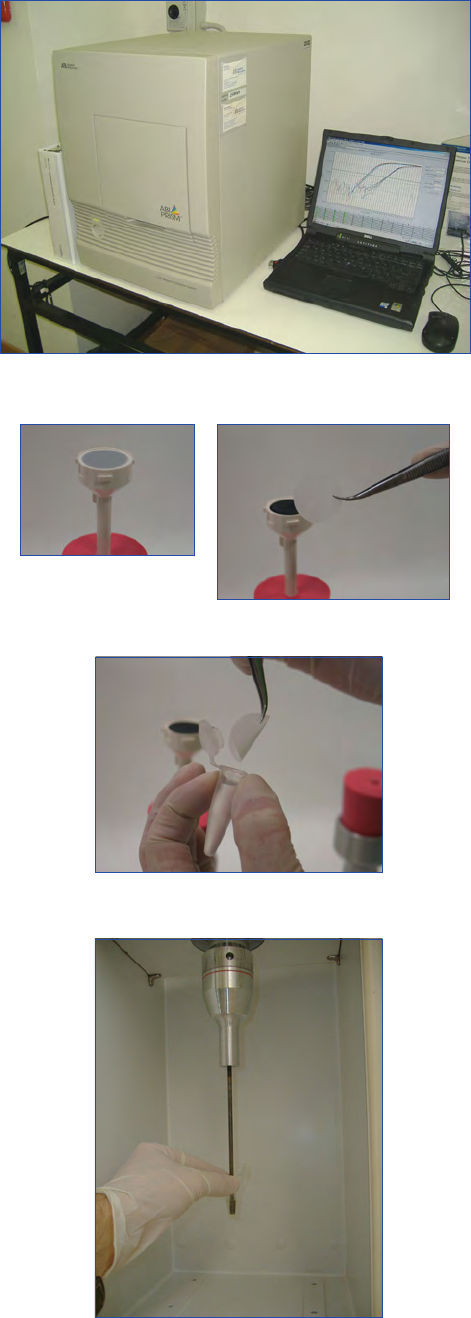
97
Microscopic and Molecular Methods for Quantitative Phytoplankton Analysis
Chapter 13 Quantitative PCR
DNA) fluorescent dyes or a number of alternative real-time
PCR chemistries which use probes (short synthetically made
pieces of DNA) which fluoresce when bound to their com-
plementary target DNA following PCR amplification (e.g.
Hydrolysis probes (TaqMan), Hybridisation probes ( FRET).
For each sample, the fluorescence signal of the reporter dye
(i.e. the dye which fluoresces in proportion to the amount of
PCR product produced) (e.g. SYBR) is divided by the fluo-
rescence signal of the passive reference dye (ROX) to obtain
a ratio defined as the normalised reporter signal (Rn). ROX
is a dye present in the reaction mix which gives out a stand-
ard level of fluorescence independent of PCR amplification.
It is used to normalise for differences in amount of reaction
mix due to pipetting errors or evaporation. Some QPCR ma-
chines do not require the use of ROX. The higher the start-
ing amount of the target molecule, the earlier a significant
increase in fluorescence (Rn value) is observed. The parameter
Ct (threshold cycle) is defined as the fractional cycle number
at which the fluorescence crosses a fixed threshold above the
baseline. The amount of target sequence in an unknown
sample is calculated by plotting the Ct value on the standard
curve. The standard curve is generated by the QPCR instru-
ment software by plotting Ct values versus the log of initial
target concentration, and by performing a linear regression.
The PCR efficiency can be calculated from the slope of the
line using the equation:
Efciency = 10
(-1/slope)
–1
If the PCR has 100% efficiency, the amount of PCR prod-
uct will double after each cycle and the slope of the standard
curve will be -3.33 (i.e. 3.33 cycles gives a 10 fold increase/
decrease between the 10 fold serial dilutions used to generate
the curves). A PCR efficiency of at least 90% (slope = 3.6) is
generally required for reliable quantitative results.
Materials
Laboratory facilities
Laboratory facilities necessary for quantitative analysis of
phytoplankton by PCR are consistent with those found in
a standard molecular biology laboratory equipped for DNA
cloning, purification, quantification and real-time (quantita-
tive) amplification.
Equipment, Chemicals and Consumables
The equipment, chemicals and consumables used in this
method are presented in the Appendix, at the end of this
chapter (Tables 1-2). Suppliers, Catalogue numbers and es-
timated cost in Euros and US Dollars are also listed in Tables
1-2.
Method
Sample processing (culture or seawater samples
fixed with acidified Lugol’s solution)
Microalgal cultures or seawater samples fixed with acidified
Lugol’s iodine solution (see chapter 2 for recipe) have to be
collected and lysed appropriately in order to generate lysates
Figure 2. Real-time PCR instrument ABI PRISM 7000 SDS (App-
lied Biosystems).
Figure 3. Filter system (A) with 3 µm Millipore TSTP mem-
brane (B).
Figure 4. Collecting cells from the filter with 1 mL artificial sterile
seawater in a 1.5 mL tube .
A B
Figure 5. Cell lysis by sonication.
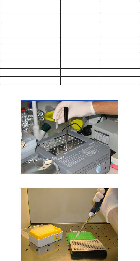
IOC Manuals & Guides no 55
Chapter 13 Quantitative PCR
98
(or starting material) suitable for use in QPCR. In many
instances the sample will need to be concentrated prior to
starting the QPCR method. This can be achieved by either
centrifugation or filtration.
Collection of Phytoplankton Cells Using a Centrifuge
1 Spin phytoplankton cells at 3000 rpm for 15 minutes
at 12 ± 1
º
C and remove the supernatant carefully. This
removes the acidified Lugol’s fixative. A swinging bucket
centrifuge is required to allow for the generation of a con-
centrated pellet.
2 Resuspend cells in a suitable volume of artificial sterile
seawater and transfer to 1.5 mL tube.
3 Spin at 3000 rpm for 15 minutes at 12 ±1
º
C in a swing-
ing bucket rotor and remove the supernatant (leaving ap-
proximately 100 µL).
4 Spin again at 10000 rpm for 10 seconds at 12 ± 1
º
C and
remove the remaining supernatant leaving the pellet in
the tube.
Collection of Phytoplankton Cells Using a Filter System
1 Filter the appropriate volume of sample to be processed
onto a 3.0 µm Millipore TSTP membrane (Fig. 3).
2 Wash the filter with 1.0 mL of artificial sterile seawater
in a 1.5 mL tube (Fig. 4). This collects the cells from the
filter surface.
3 Spin the cells at 6800 rpm for 5 minutes in a microcentri-
fuge and remove the supernatant (leaving approximately
100 µL).
4 Spin at 10000 rpm for 10 seconds and remove the re-
maining supernatant leaving the pellet dry.
Cell Lysates Preparation
1 Freeze pellet at -80 ± 1
º
C for 15 minutes.
2 Resuspend the frozen pellet with 400-600 µL lysis buffer
(PCR buffer 1X, NP40 0.5%, Tween 20 0.5%, protein-
ase K 0.1 mg mL
-1
) at a concentration of 1 x 10
5
– 2 x 10
5
cells mL
-1
.
3 Sonicate twice at 50 W for 10 seconds and incubate at 55
± 1
º
C for 2-4 hours (Figs 5-6), vortexing at intervals of
30 minutes.
4 Boil for 5 minutes and centrifuge at 12000 rpm for 2
minutes. This will eliminate cell debris and impurities.
5 Transfer the supernatant to a clean microcentrifuge tube
and store this sample lysate at -80 ± 1
º
C for 2-3 days or
process it immediately.
Standard Curve Preparation
Plasmid generation
A PCR product, generated as described previously, which
contains the complementary target DNA sequence to which
the QPCR primers bind (and probe if a probe based chem-
istry is used) is enzymatically joined at both ends (ligated) to
a specific double stranded DNA sequence called a plasmid.
This forms a circular DNA construct. A plasmid is DNA,
usually in circular form, which is capable of replicating itself
independently of cell replication. A single plasmid containing
the target sequence is introduced into a bacterial cell follow-
ing a chemical or electrical reaction. The bacteria is placed on
a nutritious gel and multiplies to form a visible colony con-
sisting of thousands of bacterial cells. The plasmid is passed
to each new cell following cell division. Within each cell, the
plasmid will also replicate many times, and with it the original
PCR product. The plasmids are purified from the bacteria re-
sulting in a highly concentrated source of pure PCR product
containing the target sequence for the QPCR assay. There are
many types of plasmids and bacterial cells commercially avail-
able and numerous methods for purification, again many of
which are incorporated into commercially available kits.
The standard curve can be constructed with 10-fold serial di-
lutions of a plasmid containing the target sequence. Usually,
the curve range extends from 1.0 × 10
2
to 1.0 × 10
6
plasmid
copies but it can be adjusted according to the assay detection
range required. The plasmid copy number is calculated using
the following formula:
Molecules µ L
-1
= (A × 6.022 × 10
23
)/(660 × B)
where: A = plasmid concentration (g µL
-1
); B = length of
the plasmid containing the cloned sequence; 6.022 × 10
23
=
Figure 6. Samples in a thermal block at 55 °C.
Figure 7. Dispersing the reaction mixtures in
the optical plate (25 µL each well).
Reagent Amount per
reaction
Final
concentration
dH
2
O variable
Commercial mix containing
SYBR Green 2X
12.5 µL 1X
*MgCl
2
25 mM 1-5 µL 1-5 mM
Forward primer 10 mM 0.25-1.5 µL 100-600 nM
Reverse primer 10 mM 0.25-1.5 µL 100-600 nM
*DNA Polymerase 5U/mL 0.125-0.25 µL 0.025-0.05 U/mL
Diluted cell lysate 1-2 µL -
Final volume 25 µL
Table 1. Master mix preparation for real-time PCR.
*Only if required. Some commercial mixes (i.e. Applied Biosys-
tems) already contain MgCl
2
and DNA polymerase
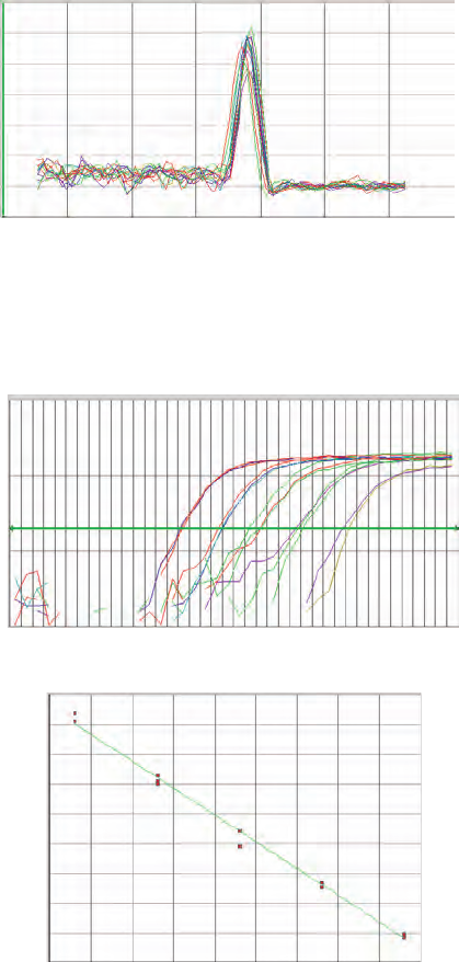
99
Microscopic and Molecular Methods for Quantitative Phytoplankton Analysis
Chapter 13 Quantitative PCR
Avogadro’s number; 660 = average molecular weight of one
base pair. The accurate determination of the plasmid con-
centration can be performed using a spectrophotometer or a
fluorimeter. Once quantified, it is recommended to store the
plasmid at -80
º
C in small aliquots to avoid repeated freeze/
thaw cycles. Moreover, plasmid dilutions should be freshly
prepared for each PCR run.
Dilutions of Sample Lysates and Plasmid
1 Make scalar dilutions 1:10 of the sample lysates with
PCR-grade H
2
O.
2 Make scalar dilutions 1:10 of the plasmid with PCR-
grade H
2
O (from 1.0 × 10
6
to 1.0 × 10
2
).
Quantitative PCR Assay
1 In a separate clean room set up the QPCR master mix
described in the Table 1. Make triplicate PCR tubes for
each lysate and plasmid dilution (see above). This is re-
quired to determine the intra-assay variability of results.
For this purpose, it is practical to aliquot a reaction vol-
ume equivalent to 3 reactions (75 µL) in one standard
PCR tube, add the template, and then disperse the reac-
tions in optical tubes/plates (25 µL per tube/well) (Fig.
7). Quantitative PCR assays are performed in a final vol-
ume of 25 µL using the SYBR Green chemistry as pre-
sented in Table 1. To reduce cost, it is possible to set up
QPCR mixtures considering a final volume of 12.5 µl
instead of 25 µl. In this case, particular care should be
taken to avoid volume differences between tubes.
2 Perform the QPCR in a real-time PCR instrument under
the following reaction conditions: 95 ºC for 5 minutes;
40 cycles of 15 sec at 95 ºC, 1 min at 60 ºC, with a
final dissociation protocol to ensure the absence of non-
specific PCR products or primer dimers (Fig. 8). These
conditions can be modified depending on the commer-
cial mix used and the characteristics of each primer.
Due to the sensitivity of the PCR method, it is crucial to
avoid contamination. It is therefore necessary to set up the
reactions in a clean area (i.e. in a PCR cabinet), free of poten-
tial plasmid or PCR product contamination. Always include
one or more negative controls (blank sample with no target
template).
PCR efficiency is important for quantification purposes: to
maximize efficiency, it is advisable to design primers produc-
ing a PCR product no more than 100 bp long. These short
amplicons can also allow the use of partially degraded DNA,
without loss of quantification performance. It is also neces-
sary to include the standard curve in each PCR run, due to
the possible variability from one PCR to another.
To avoid variability and low yields in DNA purifications,
crude cell lysates can be used as the DNA template in the
PCR reactions. These lysates contain components that can
interfere with PCR reactions and it is therefore necessary to
find a template amount which can be amplified without any
inhibitory effect. For this purpose, the QPCR assay is per-
formed, at least during the assay optimisation, with 10-fold
serial diluted lysates until quantification results become pro-
portional to sample dilutions. Usually, dilutions from 1:10 to
1:1000 are sufficient to establish the correct conditions. It is
important to note that this approach would be possible when
the target sequence is present in high copy number in the cell
(e.g. rRNA genes), otherwise the sensitivity of the method
will drop significantly.
Analysis of Results
The analysis of the results is performed using the specific
QPCR machine software.
1 Set a suitable baseline and threshold value, if the instru-
ment does not do it automatically. Plasmid amplification
plots and a standard curve similar to the one presented in
Fig. 9, should appear.
2 Using experimental results, the number of target DNA
copies per µL of the original sample can be caluclated
Temperature (C)
60 65 70 75 80 85 90 95
0.24
0.20
0.16
0.12
0.08
0.04
0.00
-0.04
Derivative
Figure 8. Example of dissociation protocol results. The graph
shows the derivative of fluorescence emission variation plotted
against the temperature increment. The peak corresponds to a
specific 173-bp PCR product. No aspecific products or primer
dimers are visible.
Figure 9. Example of standard curve obtained with a plasmid
containing 28S rDNA sequence of Alexandrium fundyense. (A)
Amplification plots with plasmid copy number from 2.0 X 10
6
to 2.0
X 10
2
. The cycle number is plotted vs the Delta Rn. The Delta Rn
represents the normalized reporter signal (Rn) minus the baseline
signal established in the early PCR cycles. Three replicates were
performed for each reference DNA sample. T: threshold. (B) Cali-
bration curve plotting log starting copy number vs Ct. Slope: –3.61;
correlation coefficient (R
2
): 0.9939.
10
1
0.1
0.01
Delta Rn
A
Cycle number
T
1 10 20 30 40
2 5.5 3 3.5 4 4.5 2.5 5 6 6.5
32
30
28
26
24
22
20
18
16
14
Ct
B
IOC Manuals & Guides no 55
Chapter 13 Quantitative PCR
100
from the standard curve.
3 In order to estimate the total number of cells in the initial
sample, the number of target DNA copies per µL in the
sample is divided by the number of rDNA copies per cell.
This is then multiplied by the initial lysate volume.
Formulas for Calculating Results:
N = [(A/B) x d] x (V/C)
N: Total number of cells in the initial sample
A: number of target DNA copies per PCR tube (calculated by
instrument software)
B: mL of cell lysate in the PCR tube
C: target DNA copies per cell (to be determined for each tar-
get species using cultured cells)
d: lysate dilution factor
V: initial lysate Volume expressed in mL
Sample Preservation and Storage
Phytoplankton samples can be preserved with acidified
Lugol’s iodine solution and stored at 4°C in the dark. Experi-
ence has shown that reliable quantitative PCR results can be
obtained from samples stored up to one year.
Discussion
The QPCR has proven to be a powerful method for the quan-
tification and detection of phytoplankton species in environ-
mental samples (Galluzzi et al. 2004, Hosoi-Tanabe and Sako
2005, Dyhrman et al. 2006).
The use of commercial PCR master mix containing interca-
lating dyes such as SYBR Green is a simple and inexpensive
approach. The assays based on intercalating dyes are very sen-
sitive, but it is noteworthy that any double stranded non tar-
get DNA can also be detected, leading to misinterpretation of
results. For this reason, the specificity of the primer is crucial.
An increase in the specificity of the assay can be obtained us-
ing a TaqMan probe but this may result in a loss of sensitivity.
Theoretically, this technique can be applied to any phy-
toplankton species with DNA sequence data available so
specific primers or probes can be designed. However, some
drawbacks need to be taken into account when applying
QPCR method to phytoplankton. In particular, when a tar-
get sequence cloned into a plasmid is used as a standard, it
is essential to know the amount of target DNA per cell, in
order to determine the cell number in the field sample. This
requires preliminary work with cultured strains to optimise
the method for each target species/strain. Due to the possi-
bility of variations of target gene copy number (particularly
in case of rRNA genes) among different strains, the level of
accuracy of the quantitative real-time PCR assays can be af-
fected, as it has been shown for Mediterranean Alexandrium
species (Galluzzi et al. in press). For this reason, the method
should be tested and optimized with the local phytoplankton
population in the geographical area to be investigated. Primer
or probe specificity needs to be tested with the local popula-
tion of phytoplankton to ensure absence of non-specific target
amplification.
Compared to classical microscopy techniques, the main ad-
vantages of the QPCR in phytoplankton monitoring include
specificity, sensitivity and applicability to preserved environ-
mental samples. Sample preservation is often necessary, but
the use of fixatives may cause the morphology distortion of
some phytoplankton species, making it more difficult to dis-
tinguish them from closely related species using a microscope.
The QPCR sample throughput can be up to 27 triplicate
samples per 96-well plate, including the standard curve. This
sample throughput may reduce working time compared to
the microscope-based methods when a high number of sam-
ples need to be analysed. It is also noteworthy that the col-
lection of phytoplankton using a filter based system is faster
then the centrifugation method. This alternative speeds up
the entire process thus reducing the handling time.
QPCR instrument prices are becoming affordable for small
research groups and are now common in many molecular bi-
ology laboratories. The consumable cost per sample has been
estimated in $4 - $6 depending on the method/master mix/
chemistry used, making the QPCR an affordable method for
monitoring purposes.
In QPCR assays, only one species or strain can be analysed
at a time unless a multiplex reaction is performed. This usu-
ally requires the use of more expensive fluorescent probes
(e.g. TaqMan probes) instead of intercalating dyes. Although
multiplexing and/or multiprobing are powerful tools for mo-
lecular investigations of specific groups of toxic algae, their
development and validation can be difficult and expensive
(Handy et al. 2006).
This method can be still considered at the developmental
stage. If this method is incorporated into future monitoring
programs for HAB-species, a subset of samples could also be
checked using a more traditional microscopic technique. This
type of quality control would validate the presence of the tar-
get species on a selected subset of samples and highlight any
problems that may arise with the method.
Acknowledgements
EU-Project Seed GOCE-CT-003875-2005.
References
Bowers HA, Tengs T, Glasgow HB, Burkhoelder JMj, Rublee PA,
Oldach DW (2000) Development of real-time PCR assay for rap-
id detection of Pfiesteria piscicida and related dinoflagellates. Appl
Environ Microbiol 66:4641-4648
Coyne KJ, Cary SC (2005) Molecular approaches to the investiga-
tion of viable dinoflagellate cysts in natural sediments from estua-
rine environments. J Eukaryot Microbiol 52:90-94
Coyne KJ, Handy SM, Demir E, Whereat EB, Hutchins DA, Por-
tune KJ, Doblin MA, Cary SC (2005) Improved quantitative real-
time PCR assays for enumeration of harmful algal species in field
samples using an exogenous DNA reference standard. Limnol
Oceanogr Methods 3:381–391
Dyhrman ST, Erdner D, La Du J, Galac M, Anderson DM (2006)
Molecular quantification of toxic Alexandrium fundyense in the
Gulf of Maine using real-time PCR. Harmful Algae 5:242–250
Galluzzi L, Penna A, Bertozzini E, Vila M, Garcés E, Magnani M
101
Microscopic and Molecular Methods for Quantitative Phytoplankton Analysis
Chapter 13 Quantitative PCR
(2004) Development of Real-Time PCR assay for rapid detection
and quantification of A. minutum (Dinoflagellate). Appl Environ
Microbiol 70:1199-1206
Handy, SM, Hutchins, DA, Cary, SC, Coyne, KJ, (2006)
Simultaneous enumeration of multiple raphidophyte species by
quantitative real-time PCR: capabilities and limitations. Limnol.
Oceanogr. Methods 4: 193–204
Hosoi-Tanabe S, Sako Y (2005) Species-specific detection and quanti-
fication of toxic marine dinoflagellates Alexandrium tamarense and
A. catenella by Real-Time PCR assay. Mar Biotechnol 7:506-514
Kamikawa R, Hosoi-Tanabe S, Nagai S, Itakura S, Sako Y (2005)
Development of a quantification assay for the cysts of the toxic
dinoflagellate Alexandrium tamarense using real-time polymerase
chain reaction. Fish Sci 71: 987–991
Park TG, de Salas MF, Bolch CJ, Hallegraeff GM (2007) Develop-
ment of a real-time PCR probe for quantification of the hetero-
trophic dinoflagellate Cryptoperidiniopsis brodyi (Dinophyceae) in
environmental samples. Appl. Environ. Microbiol. 73: 2552–2560
Popels LC, Cary SC, Hutchins DA, Forbes R, Pustizzi F, Gobler
CJ, Coyne KJ (2003) The use of quantitative polymerase chain
reaction for the detection and enumeration of the harmful alga
Aureococcus anophagefferens in environmental samples along the
United States East Coast. Limnol Oceanogr: Methods 1:92–102
Touzet N, Keady E, Raine R, Maher M (2009) Evaluation of taxa-
specific real-time PCR, whole-cell FISH and morphotaxonomy
analyses for the detection and quantification of the toxic
microalgae Alexandrium minutum (Dinophyceae), Global Clade
ribotype. FEMS Microbial Ecol. 67:329-341

IOC Manuals & Guides no 55
Chapter 13 Quantitative PCR
102
Appendix
Table 1. Equipment and suppliers.
Table 2. Chemicals and suppliers.
*Different commercial SYBR Green mixtures can also be used (for example
Hot-Rescue Real Time PCR KIT-SG from Diatheva, Italy).
Equipment Supplier Cat. Number
€
US $
Real-time PCR instrument ABI PRISM 7300 SDS Applied Biosystems 4351101 29840 42099
Ultrasonic Homogeniser Branson S-150D VWR international 33995 2110 2980
Analog Dry Block Heater VWR international 12621-110 344 485
Swing-bucket Centrifuge IEC-CL30 Thermo Scientific 11210904 5532 7856
Mini-Centrifuge Heraeus ”Biofuge Fresco” Thermo Scientific 75002420 3600 5110
Spectrophotometer Shimadzu, Japan UV-2401 PC 8000 11360
Sum approx. 49426 69890
Chemicals/consumables Supplier Cat. Number
€
US $
Isopore membrane filter 3.0 µm TSTP Millipore, USA TSTP02500 129 183
Lugol solution (1L) Sigma-Aldrich Srl, Italy 62650 26 37
*SYBR Green PCR Master Mix, 2 X 200 reactions Applied Biosystems, USA 4364344 664 936
MicroAmp Optical 96-well Reaction Plate, 20/pkg Applied Biosystems, USA 4306737 152 214
Optical Adhesive Covers, 25/pkg Applied Biosystems, USA 4360954 76 107
Tween 20 Sigma-Aldrich Srl, Italy P1379-100ML 26.9 38
NP 40 Sigma-Aldrich Srl, Italy 74385-1L 36 50
Proteinase k Sigma-Aldrich Srl, Italy P6556-25MG 39.1 55
Primers forward and reverse (25 nmol) Invitrogen, Italy - 13 18
Tubes 1.5 mL Sarstedt, Germany 72690 - 500/pack 16 22
Polypropylene conical tubes 50 mL BD Biosciences 352070 - 500/case 99 140
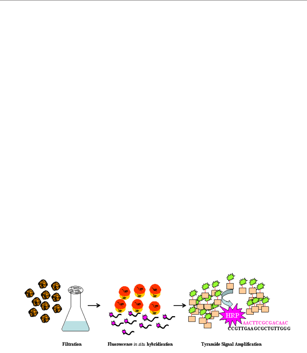
103
Microscopic and Molecular Methods for Quantitative Phytoplankton Analysis
Chapter 14 Tyramide signal amplification in combination with fluorescence in situ hybridisation
Introduction
Tyramide Signal Amplification (TSA) - Fluorescence in situ
Hybridisation (FISH) provides an enhanced fluorescence sig-
nal from molecular probes The oligonucleotide probe is la-
belled with the enzyme horseradish peroxidase (HRP). After
hybridisation the HRP catalyses the deposition of a phenolic
compound, a FITC (fluorescein isothiocyanate) labelled tyra-
mide. In the presence of hydrogene peroxide, the immobi-
lised tyramide binds to electron rich moieties (mostly tyrosine
residues) of adjacent proteins. This TSA reaction results in a
signal enhancement of up to 30 times more intensity then
traditional labelled fluorescent probes (Fig. 1).
Solid phase cytometry
Solid phase cytometry (SPC) combines the advantages of flow
cytometry with image analysis (Kamentsky 2001), and enables
the fast detection and enumeration of micro-organisms down
to one cell in a sample (Lemarchand et al. 2001). In SPC, the
laser is moved over cells immobilised onto a solid support,
which allows the rapid enumeration of several thousand cells
with a similar accuracy to flow cytometry (Darynkiewicz et al.
2001). The ChemScan™ instrument (Chemunex, France) is
a SPC, which was initially developed for industrial and envi-
ronmental microbiology (Mignon-Godefroy et al. 1997, Rey-
nolds and Fricker 1999). It was adapted for the detection of
toxic microalgae using antibody (West et al. 2006) and oligo-
nucleotides probes (Töbe et al. 2006). The ChemScan™ uses
a 488 nm argon-ion laser and is therefore suited for probes
or tyramides labelled with FITC. Algal cells are collected by
filtration onto a polycarbonate membrane, hybridised, and
subsequently scanned (Fig. 2). Fluorescent events are detected
and a computer applies various criteria to discriminate be-
tween “true” and “false” signals deriving from hybridised cells
using the MatLab-based software (Matworks, Natick, USA)
for comparison with Gaussian curves (Roubin et al. 2002).
The exact positions of positively identified cells are shown as
14 Tyramide signal amplification in combination
with fluorescence in situ hybridisation
Kerstin Töbe
1
*
1
Alfred Wegener Institute for Polar and Marine Research Am Handelshafen 12. D-27570 Bremerhaven, Germany
*Author for correspondence e-mail: Kerstin.T[email protected]
coloured spots on a display of the membrane in a scan map.
The hybridised cells can be visualised by transferring the
membrane with its membrane holder to an epifluorescence
microscope equipped with a computer controlled motorised
stage that is connected to the ChemScan™. This allows each
positive data point to be visually validated by microscopic ex-
amination immediately after scanning as true positives or false
positives (Reynolds and Fricker 1999, Roubin et al. 2002).
This method is very fast, positive hybridised cells are counted
within 3 minutes and no positive hybridised cell can be over-
looked by the operator as in standard FISH applications.
TSA-FISH is required for reliable automated detection of
target cells with the ChemScan™ to increase the peak fluo-
rescence intensity as a discrimination pattern in the compu-
ter software. Since TSA-FISH labelled cells reach very high
fluorescence intensities, this allows the computer software to
develop discrimination patterns between labelled and non-la-
belled cells. This new automated method for counting micro-
algae is, however, only adequate for round and spherical cells
at the moment and not for long colony forming species, like
the diatoms Pseudo-nitzschia. The computer software present-
ly used must be revised in order to count filamentous colony
forming microalgae. Microscopic verification of positive cells
is recommended. This can be performed after confirming that
the FISH labelling has been successfully completed.
Presently, the application of only one single probe label is pos-
sible, because of the single laser of the ChemScan™ and it is
therefore not possible to detect more than one species on a
filter at a time. The effectiveness of a new probe label is, how-
ever, under development. This new probe label is excited with
the present ChemScan™ laser, like standard FITC-labelled
cells, but it has a different emission wavelength and with the
installation of a suited Photomultiplier, two different probes
could be applied.
Figure 1. Tyramide signal amplification.

IOC Manuals & Guides no 55
Chapter 14 Tyramide signal amplification in combination with fluorescence in situ hybridisation
104
Scope
Semi-automated detection and quantification of target phyto-
plankton species.
Detection range
Detection of microalgal RNA by FISH is very sensitive. The
number of cells that can be detected depend on the sample vo-
lume. High biomass can obscure the view of target cells.
Advantages
Simple and easy to use. Sample volumes can easily be adjusted.
Simultaneous labeling and detection of multiple species is pos-
sible. Strong yellowish/green labelling of target cells minimises
confusion with non-target cells. Semi-automated analysis.
Drawbacks
Probes are only available for a limited number of target species.
Rigorous optimisation and specificity testing on local strains is
required before the method can be implemented. Finite storage
time for samples. Complex sample processing procedure may
result in cell loss. At present very high start-up costs. Intensity
of positive reaction may vary with cell conditions. Access to
molecular expertise is essential. Appropriate laboratory facilities
for storage and processing of probes and reagents are necessary.
Type of training needed
Instruction in setting up this technique should come from a
person with an in-depth knowledge and experience of mole-
cular biology. Approximately one week of supervised training
required to properly perform the method.
Essential Equipment
Solid phase cytometer and epifluorescence microscope with
automated stage; filtration unit, vacuum pump, hybridisation
oven.
Equipment cost*
Total set-up cost = €183310, $ 269.795
See Appendix, Table 1 for details
Consumables, cost per sample**
€11 ($16.13), see also Appendix, Table 2
Processing time per sample before analysis
5-30 minutes. Filtering time depends on the amount of phyto-
plankton in the samples.
Analysis time per sample
The TSA-FISH procedure and analysis with SPC requires 4.25
hours of handling time per filter of 3 minutes for scanning and
2 minutes for verification of the results.
Sample throughput per person per day
A trained person can process up to 36 samples per day depen-
ding on the number of target organisms in each sample.
No. of samples processed in parallel
36
Health and Safety issues
Relevant health and safety procedures must be followed. The
following chemical is particularly hazardous: Formamide.
*service contracts not included
**salaries not included
The fundamentals of
The tyramide signal amplification - fluoresence in situ hybridisation in combination with solid
phase cytometry method
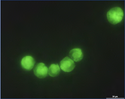
105
Microscopic and Molecular Methods for Quantitative Phytoplankton Analysis
Chapter 14 Tyramide signal amplification in combination with fluorescence in situ hybridisation
Materials
Laboratory facilities
Molecular biology laboratory
Required Equipment (essential)
The quantitative TSA-FISH in combination with solid phase
cytometry requires the following equipment:
• Solid phase cytometer
• Epifluorescence microscope with motorised stage
• Filter vacuum manifold or glass filter equipment
• Hybridisation oven
• Vacuum pump
• Pipettes 1-20 µL, 100-100 µL + sterile tips, 1-50 mL pi-
pette + sterile tips
• Autoclaved glassware
• Disposable gloves, tweezers,
• White polycarbonate filter membranes: 25 mm diameter,
pore size depending on cell size
• Support pads
Chemicals and Consumables
Solutions for Fixation
Saline ethanol (Scholin et al. 1996), prepared freshly for each
experiment because of the formation of precipitates
25 vol. 95 % ethanol
2 vol. Milli-Q water
3 vol. 25X SET
or modified saline ethanol (Miller and Scholin 2000) stable
at room temperature for several months without precipitate
formation
22 vol. 95 % ethanol
5 vol. Milli-Q water
3 vol. 25X SET buffer
25X SET
3.75 M NaCl
0.5 M Tris/HCl
25 mM EDTA
pH 7.8, filter sterilised
Solutions for Fluorescence In situ Hybridisation
Hybridisation buffer
0.1 % (v/v) Nonidet-P40 (Sigma N-6507)
x % (v/v) Formamide
2 % blocking reagent (Roche, Mannheim, Germany)
Wash buffer:
1X SET
Solution for quenching endogenous peroxidase activity
3 % Hydrogene peroxide (H
2
O
2
) in filter sterilised deionised
water
Solutions for amplification reaction
TNT-Buffer
0.1 M Tris-HCL, pH 7.5
0.15M NaCl
0.05 % Tween 20
Tyramide substrate solution
One volume of 40 % (wt/vol) dextrane sulfate (Sigma-Aldrich,
Munich, Germany) in sterile deionised water, is mixed with
one volume of amplification diluent and a 1:50 dilution of
the fluorescein labelled tyramide (Perkin Elmer, Boston Ma,
USA, diluted in Dimethylsulfoxide) in sterile deionised water
and stored in the dark.
Solution for counterstaining
Citifluor/DAPI (4’,6’-diamidino-2-phenylindoline) mixture
(0.5 mL sterile deionised water, 1 mL Citifluor (Citifluor
Ltd., Cambridge) and 1.5 µL DAPI solution (1 µg µL
-1
, Inv-
itrogen, Germany, in sterile deionised water)).
Probes
Horseradish peroxidase labelled probes purchased from Ther-
mo Scientific, Germany are delivered lyophilized. The HRP-
label is anchored at the 5’-end of the oligonucleotide. Stock
solution of 1 µg µL
-1
, and working solutions of 500 µL
-1
and
50 ng µL
-1
should be prepared in 1X TE buffer, pH 7.8- 8.0.
Probe stock solution should be stored at -80°C and working
solutions at -20°C. Since, HRP-labelled probes are not light
sensitive it is not necessary to work in the dark. However,
from the tyramide signal amplification step on working in
the dark is necessary, because of the incorporated light sensi-
tive FITC-labelled tyramide. More information on the equip-
ment, chemicals and consumables used in this method are
presented in the Appendix at the end of this chapter.
Method
Handling Time
Based on 10 samples processed in parallel
0.5 h Set-up and filtering step
1 h Fixation
0.25 h Wash step and probe addition
1.5 h Hybridisation and tyramide signal amplification
0.5 h Analysis of 10 filter with solid phase cytometer
0.5 h Clean up
TOTAL HOURS 4.25 h
Figure 2. Tyramide Signal Amplification FISH with Alexandrium
fundyense cells and HRP-labelled probe ATNA02 (John et al.
2005), photographed at 40x objective lens.

IOC Manuals & Guides no 55
Chapter 14 Tyramide signal amplification in combination with fluorescence in situ hybridisation
106
Sample Preservation and Storage
• Filter 5 mL sample onto a polycarbonate filter with the
lowest possible vacuum and incubate in the fixative for at
least 1 hour at room temperature or overnight at 4 ºC.
• Remove the fixative by filtrating and incubating for 5 mi-
nutes with hybridisation buffer without a probe.
Filters can be dried and stored for at least one month at room
temperature or hybridised directly afterwards.
Quenching of Natural Occurring Peroxidases
• Quench naturally occurring endogenous peroxidase ac-
tivity by treating the filters with 100 µL 3 % H
2
O
2
per
filter at room temperature for 15 to 30 minutes to avoid
unspecific staining.
• Rinse the filter in sterile deionised water to remove excess
H
2
O
2
.
Hybridisation
• Cover the filters with 80-100 µL hybridisation buffer
containing the horse radish peroxidase labelled probe
(final concentration of probe in hybridisation buffer:
5 ng µL
-1
) and hybridise 1.5-2 hours at 37 ºC.
• Stop the hybridisation by adding pre-warmed (37 ºC) 1X
SET wash buffer and then wash the filters with 1X SET
for 10 minutes at 37 ºC.
Tyramide Signal Amplification
• Equilibrate the filters for 15 minutes in TNT buffer at
room temperature.
• Remove excess liquid by putting the filters on blotting
paper, staining should be conducted before they are com-
pletely dry.
• Incubate each filter with 100 µL Tyramide substrate solu-
tion for approximately 30 minutes at room temperature
in the dark.
• Rinse the filters in TNT-buffer and wash for 15 minutes
at 55 ºC in TNT-buffer. Then rinse the filter in sterile
deionised water, air dry and store at -20 ºC pending ana-
lysis by ChemScan™.
Optional Step
Counterstaining
• Counterstain the filters with a Citifluor/DAPI mixture
for 10 minutes at room temperature. Wash with sterile
deionised water for 1 minute and incubate in 80 % etha-
nol (v/v) for 30 seconds to remove an excess of staining
solution. Air Dry and store at -20 ºC or examine directly
with the ChemScan™. Citifluor is used as an antifade
and the blue DAPI nucleic acid stain effectively stains
double stranded DNA and enables a general overview of
all cells on a hybridised filter.
Formulas for Calculating Results
The entire filter is automatically counted by the solid phase
cytometer and afterwards validated randomly by the operator.
Hence the cell number is reflective of the amount of original
sample that was processed and preserved as well as a the vol-
ume that was filtered for hybridisation.
To calculate cells L
-1
:
where N is the number of positive cells on the whole filter and
V (mL) is the volume of sample used.
Analysis of hybridised filters with SPC in combi-
nation with epifluorescence microscopy
The ChemScan™ system (Fig. 3) must be calibrated on a
daily basis with a standardised amount of FITC labelled latex
beads, diameter 2-3 µm (Standard C, Chemunex, France), in
100 µL. In order to verify that the laser is working properly,
the number of fluorescence signals recorded by the Chem-
Scan™ must be cross referenced with the number of counted
latex beads in solution.
1. The 100 µL solution with the latex beads is filtered onto
a black polycarbonate membrane (25 mm diameter, 0.2
µm pore size, Chemunex, France). To support the filter
membrane, a black support pad is mounted by applying
100 µL ChemSol B16 (Chemunex, France) to a mem-
brane holder. Then the filter membrane with latex beads
is laid onto the support pad. The filter is scanned with
the application C control.
2. For TSA-FISH filter also a black support pad is mounted
by applying 100 µL ChemSol B16 (Chemunex, France),
overlaid by the hybridised filter and the the application
tvcbio1 (tvc: total viable counts) is used. The peak inten-
sity is manually changed from 250 to 2500 to prevent
the enumeration of false positive autofluoresing particles
with lower peak fluorescence intensity.
3. Immediately after the scan, signals are validated using
an epifluorescence microscope (Nikon, Eclipse E 800)
equipped with filter blocks for FITC (Nikon Filter Block
B-2A) and DAPI (Nikon Filter Block UV-2A) and with
a motorised stage (Prior Scientific, UK). Images are cap-
tured with a digital camera (CCD-1300CB, Vosskühler,
Germany) and analysed with the Nikon software Lucia
G.
Discussion
Traditional FISH methods have limitations when counting
samples with low target cell densities as well as in the number
of samples that can be analysed per day. The time involved to
count an environmental sample will vary with the diversity
of the sample and the skill of the operator. For a high sample
throughput, FISH has been combined with flow cytometry,
which allows the analysis of different cell parameters.
However, a combination of flow cytometry and microscopy of
single detected fluorescent microalgae is difficult. In addition,
because of the limited sensitivity at lower cell concentrations
this method is not suited for the detection of cells at low
concentrations in environmental samples. The solid phase
−
1000 *
)(
)(
) (
1
=
mLsampleofVolume
NfilterwholeoncountcellPositive
Lcells ion concentrat Cell
−
1000 *
)(
)(
) (
1
=
mLsampleofVolume
NfilterwholeoncountcellPositive
Lcells ion concentrat Cell
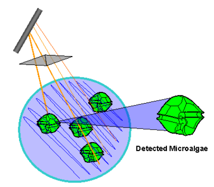
107
Microscopic and Molecular Methods for Quantitative Phytoplankton Analysis
Chapter 14 Tyramide signal amplification in combination with fluorescence in situ hybridisation
cytometer has the advantage of a direct combination of
automated counting and epifluorescence microscopy, allowing
the microscopically verification of each single cell detected.
The solid phase cytometry in combination with TSA-FISH
enables the efficient detection of a single cell in a filtered
volume in less than 5 h. For a reliable automated detection
of target cells with the ChemScan™, signal amplification is
necessary. This method has great potential for application in
analysing field material where a rapid and reliable detection
and enumeration of target cells is required. The shape of the
algae may cause problems, e.g., the ChemScan™ cannot
count long chain forming cells like Pseudo-nitzschia cells. The
adaptation of improved software could help to overcome this
problem. Additionally, the actual high price of this machine
and the additional costs of an epifluorescence microscope
equipped with an automatic stage is a limiting factor.
Acknowledgements
The work was funded by the Stiftung Alfred-Wegener-Insti-
tut für Polar und Meeresforschung in the Helmholtz-Ges-
ellschaft, Bremerhaven, Germany, in part by EU DETAL ,
project QLRT-1999-30778 and Chemunex, Ivry, France.
Figure 3. Overlapping scan with the ChemScan.
References
Darynkiewicz Z, Smolewski P, Bedner E (2001) Use of flow
and laser scanning cytometry to study mechanisms regulat-
ing cell cycle and controlling cell death. Clin Chem Lab
Med 21:857-873
John U, Medlin LK, Groben R (2005) Development of spe-
cific rRNA probes to distinguish between geographic clades
of the Alexandrium tamarense species complex. J Plankton
Res 27:199-204
Kamentsky LA (2001) Laser scanning cytometry. Methods
Mol Cell Biol 63:51-87
Lemarchand K, Parthuisot N, Catala P, Lebaron P (2001)
Comparative assessment of epifluorescence microscopy,
flow cytometry and solid-phase cytometry used in the enu-
meration of specific bacteria in water. Aquat Microb Ecol
25:301-309
Mignon-Godefroy K, Guillet JC, Butor C (1997) Laser scan-
ning cytometry for the detection of rare events. Cytometry
27:336-344
Miller PE, Scholin CA (2000) On detection of Pseudo-nitzschia
(Bacillariophyceae) species using whole cell hybridization: Sample
fixation and stability. J Phycol 36:238-250
Roubin MR, Pharamond JS, Zanelli F, Poty F, Houdart S,
Laurent F, Drocourt, JL, Van Poucke S (2002) Application
of laser scanning cytometry followed by epifluorescent and
differential interference contrast microscopy for the detec-
tion and enumeration of Cryptosporidium and Giardia in
raw and potable waters. J Appl Microbiol 93:599-607
Reynolds DT, Fricker CR (1999) Application of laser scan-
ning for the rapid and automated detection of bacteria in
water samples. J Appl Microbiol 86:785-795
Scholin CA, Buck KR, BritschigT, Cangelosi G, Chavez FP
(1996) Identification of Pseudo-nitzschia australis (Bacillari-
ophyceae) using rRNA-targeted probes in whole cell and
sandwich hybridization formats. Phycologia 35:190-197
Töbe K, Eller G, Medlin LK (2006) Automated detection
and enumeration of Prymnesium parvum (Haptophyta:
Prymnesiophyceae) by solid-phase cytometry. J Plankton
Res 28:643-657
West NJ, Bacchieri R, Hansen G, Tomas C, Lebaron P,
Moreau H (2006) Rapid quantification of the toxic alga
Prymnesium parvum in natural samples by use of a specific
monoclonal antibody and solid-phase cytometry Appl En-
vir Microbiol 72:860-868

IOC Manuals & Guides no 55
Chapter 14 Tyramide signal amplification in combination with fluorescence in situ hybridisation
108
Appendix
Table 1. Equipment and suppliers.
Table 2. Chemicals and suppliers.
Equipment Supplier Cat. Number
€
US $
Filter Manifold Millipore, USA XX2702550 400 587
Vacuum pump Omnilab, Germany 9.881 391 574
Incubator ”Shake’n’Stack” VWR, Germany 7996 2310 3387
Epifluorescence microscope, e.g. Nikon
Eclipse E800 with motorized stage
Nikon, Japan MAA600BA 29000 42521
Solid phase cytometer e.g. ChemScan™ Chemunex, France 152000 222870
Chemicals Supplier Cat. Number
€
US $
Ethanol, absolute, 1L Merck 1.009.832.500 73 107
Milli-Q water Most labs have an in-
house supply
Sodium chloride, 1 kg Sigma-Aldrich S9888 23 34
Tris/HCl, 500 g Sigma-Aldrich T3253 96 141
Nonidet-P40, 100 mL Roche 11754599 74 109
EDTA, 500 g Sigma-Aldrich E7889 56 82
Isopore white polycarbonate membrane
filter, 3 µm pore size, Qty. 100
Millipore TSTP02500 130 191
Hydrogene peroxide Pharmacy - 4 6
HRP-labelled probe, approx. 300 µg Thermo Scientific - 235 345
Deionized formamide, 100 mL Sigma-Aldrich F 9037 46 67

109
Microscopic and Molecular Methods for Quantitative Phytoplankton Analysis
Appendix: Acronyms and Notation
Acronym Meaning
ABD Area-Based spherical Diameter
ADPA N-Phenyl-1,4-benzenediamine hydrochloride
ALGADEC Development of a RNA -Biosensor for the Detection of Toxic Algae
approx. Approximately
ARB “arbor ”=tree
BSA Bovine Saline A
CCD Charge Coupled Device
CEN Comité Europeén De Normalisation
ChemScan™ Lazer scanning Process Analyser/solid-phase cytometry (Scan RDI™ in North America)
Chl a Chlorophyll a
CICEET Cooperative Institute for Coastal and Estuarine Technology
CPR Continuous Plankton Recorder
CTD Conductivity, Temperature, Depth
dH
2
O distilled water
DAPI 4’,6-diamidino-2-phenylindoline
DIC Differential interference contrast
DICANN Dinoflagellate Categorisation by Artificial Neural Network
DSP Diarrhetic Shellfish Poisoning
ECOHAB The Ecology and Oceanography of Harmful Algal Blooms
EPA Environmental Protection Agency
ESD Equivalent Spherical Diameter
ESP Environmental Sample Processor
EU European Union
EU DETAL Rapid and ultra-sensitive fluorescent test for the tracking of toxic algae in the marine environment
FISH Fluorescence In Situ Hybridisation
FIT Fluid Imaging Technologies
FITC Fluorescein isothiocyanate
FlowCAM Flow Cytometer And Microscope
FSW Filtered Sea Water
FTF Filter-Transfer-Freeze
GF/F Glass Fibre Filters
HAB(s) Harmful Algal Bloom(s)
HAB Buoy Harmful Algal Bloom Buoy
HAE(s) Harmful Algal Event(s)
Hybe Hybridisation
ICES International Council for the Exploration of the Sea
IOC Intergovernmental Oceanographic Comission of UNESCO
LED Light-Emitting Diode
LM Light Microscopy
LSU Large SubUnit
MBARI Monterey Bay Aquarium Research Institute
NASA National Aeronautics and Space Administration
NOAA National Oceanic and Atmospheric Administration
NSF National Science Foundation
ONR Office of Naval Research
PCR Polymerase Chain Reaction
PFA Paraformaldehyde
PICODIV Picoplankton Diversity
PSP Paralytic Shellfish Poisoning
QC Quality Control
rDNA Ribosomal Deoxyribonucleic Acid
RNases Ribonucleases
rRNA Ribosomal Ribonucleic Acid
RT-PCR Real-Time PCR
Please note that RT-PCR usually refers to reverse transcriptase PCR, In this manual the acronym
refers to Real Time PCR.
SEM Scanning electron Microscopy
SOP Standard Operating Procedure
SSU Small SubUnit
TEM Transmission Electron Microscopy
TSA-FISH Tyramide Signal Amplification has been used with FISH
UNESCO United Nations Educational Scientific and Cultural Organisation
wt/vol weight/volume
IOC Manuals & Guides no 55
110
SI Unit Meaning
I
2
Iodine
KI Potassium Iodide
mL millilitre
L Litre
cm Centimetre
hr Hour
ºC Degree Celsius
% Percentage
µm Micrometre
mm
2
Millimetre squared
Min
-1
Per minute
Hg Mercury
n Number
g Gram(s)
µL Microlitres
v/v Volume to volume
x g Multiplied by gravity
113
Microscopic and Molecular Methods for Quantitative Phytoplankton Analysis
List of previous titles in the series continued:
19 Guide to IGOSS Specialized Oceanographic Centres (SOCs). 1988. 17 pp. (English, French, Spa-
nish, Russian)
20 Guide to Drifting Data Buoys. 1988. 71 pp. (English, French, Spanish, Russian)
21 (Superseded by IOC Manuals and Guides No. 25)
22 GTSPP Real-time Quality Control Manual. 1990. 122 pp. (English)
23 Marine Information Centre Development: An Introductory Manual. 1991. 32 pp. (English, French,
Spanish, Russian)
24 Guide to Satellite Remote Sensing of the Marine Environment. 1992. 178 pp. (English)
25 Standard and Reference Materials for Marine Science. Revised Edition. 1993. 577 pp. (English)
26 Manual of Quality Control Procedures for Validation of Oceanographic Data. 1993. 436 pp. (Eng-
lish)
27 Chlorinated Biphenyls in Open Ocean Waters: Sampling, Extraction, Clean-up and Instrumental
Determination. 1993. 36 pp. (English)
28 Nutrient Analysis in Tropical Marine Waters. 1993. 24 pp. (English)
29 Protocols for the Joint Global Ocean Flux Study (JGOFS) Core Measurements. 1994. 178 pp .
(English)
30 MIM Publication Series:
Vol. 1: Report on Diagnostic Procedures and a Definition of Minimum Requirements for Providing
Information Services on a National and/or Regional Level. 1994. 6 pp. (English)
Vol. 2: Information Networking: The Development of National or Regional Scientific Information
Exchange. 1994. 22 pp. (English)
Vol. 3: Standard Directory Record Structure for Organizations, Individuals and their Research
Interests. 1994. 33 pp. (English)
31 HAB Publication Series:
Vol. 1: Amnesic Shellfish Poisoning. 1995. 18 pp. (English)
32 Oceanographic Survey Techniques and Living Resources Assessment Methods. 1996. 34 pp.
(English)
33 Manual on Harmful Marine Microalgae. 1995. (English) [superseded by a sale publication in 2003,
92-3-103871-0. UNESCO Publishing]
34 Environmental Design and Analysis in Marine Environmental Sampling. 1996. 86 pp. (English)
35 IUGG/IOC Time Project. Numerical Method of Tsunami Simulation with the Leap-Frog Scheme.
1997. 122 pp. (English)
36 Methodological Guide to Integrated Coastal Zone Management. 1997. 47 pp. (French, English)
37 Post-Tsunami Survey Field Guide. First Edition. 1998. 61 pp. (English, French, Spanish, Russian)
38 Guidelines for Vulnerability Mapping of Coastal Zones in the Indian Ocean. 2000. 40 pp. (French,
English)
39 Manual on Aquatic Cyanobacteria – A photo guide and a synopsis of their toxicology. 2006. 106
pp. (English)
40 Guidelines for the Study of Shoreline Change in the Western Indian Ocean Region. 2000. 73 pp.
(English)
41 Potentially Harmful Marine Microalgae of the Western Indian Ocean. Microalgues potentiellement
nuisibles de l’océan Indien occidental. 2001. 104 pp. (English/French)
42 Des outils et des hommes pour une gestion intégrée des zones côtières - Guide méthodologique,
vol.II/Steps and Tools Towards Integrated Coastal Area Management – Methodological Guide, Vol.
II. 2001. 64 pp. (French, English; Spanish)
43 Black Sea Data Management Guide (Cancelled)
44 Submarine Groundwater Discharge in Coastal Areas – Management implications, measurements
and effects. 2004. 35 pp. (English)
IOC Manuals & Guides no 55
114
45 A Reference Guide on the Use of Indicators for Integrated Coastal Management. 2003. 127 pp.
(English). ICAM Dossier No. 1
46 A Handbook for Measuring the Progress and Outcomes of Integrated Coastal and Ocean Mana-
gement. 2006. iv + 215 pp. (English). ICAM Dossier No. 2
47 TsunamiTeacher – An information and resource toolkit building capacity to respond to tsunamis
and mitigate their effects. 2006. DVD (English, Bahasa Indonesia, Bangladesh Bangla, French,
Spanish, and Thai)
48 Visions for a Sea Change. Report of the first international workshop on marine spatial planning.
2007. 83 pp. (English). ICAM Dossier No. 4
49 Tsunami preparedness. Information guide for disaster planners. 2008. (English, French, Spanish)
50 Hazard Awareness and Risk Mitigation in Integrated Coastal Area Management. 2009. 141 pp.
(English). ICAM Dossier No. 5
51 IOC Strategic Plan for Oceanographic Data and Information Management (2008–2011). 2008. 46
pp. (English)
52 Tsunami risk assessment and mitigation for the Indian Ocean; knowing your tsunami risk – and
what to do about it. 2009. 82 pp. (English)
53 Marine Spatial Planning. A Step-by-step Approach. 2009. 96 pp. (English). ICAM Dossier No. 6
54 Ocean Data Standards Series:
Vol. 1: Recommendation to Adopt ISO 3166-1 and 3166-3 Country Codes as the Standard for
Identifying Countries in Oceanographic Data Exchange. 2010. 13 pp. (English)
55 Microscopic and Molecular Methods for Quantitative Phytoplankton Analysis. 2010. 114 pp. (Eng-
lish)

The Intergovernmental Oceanographic Commission (IOC) of UNESCO celebrates its 50th anniversary in 2010. Since taking the
lead in coordinating the International Indian Ocean Expedition in 1960, the IOC has worked to promote marine research, protection
of the ocean, and international cooperation. Today the Commission is also developing marine services and capacity building, and is
instrumental in monitoring the ocean through the Global Ocean Observing System (GOOS) and developing marine-hazards warning
systems in vulnerable regions. Recognized as the UN focal point and mechanism for global cooperation in the study of the ocean, a
key climate driver, IOC is a key player in the study of climate change. Through promoting international cooperation, the IOC assists
Member States in their decisions towards improved management, sustainable development, and protection of the marine environment.
