
SBCUSD – IT Training Program
MS Excel ll
Fill Downs, Sorting, Functions, and More
Revised – 4/16/2019

Excel ll – Fill Downs, Sorting, Functions, and More
1
TABLE OF CONTENTS
Number Formats ........................................................................................................................................................4
Auto Fill and Flash Fill .................................................................................................................................................5
Simple Repeat .........................................................................................................................................................5
Fill Down Common Series .......................................................................................................................................5
Fill Down Custom Series .........................................................................................................................................5
Flash Fill Series ........................................................................................................................................................5
Sorting ........................................................................................................................................................................7
Basic Sorting – Single Column ................................................................................................................................7
Sort Multiple Columns ............................................................................................................................................7
Sort Custom Order ..................................................................................................................................................7
Filtering .......................................................................................................................................................................8
Filtering by Value ....................................................................................................................................................8
Multiple Filters .......................................................................................................................................................8
Conditional Filtering ...................................................................................................................................................9
Basic Functions and Formula Development ............................................................................................................ 10
Formula Basics ..................................................................................................................................................... 10
Formula Syntax .................................................................................................................................................... 10
Referencing Cell Ranges in Formulas .................................................................................................................. 10
Common Functions .................................................................................................................................................. 11
Sum ...................................................................................................................................................................... 11
Average ................................................................................................................................................................ 11
Min....................................................................................................................................................................... 11
Max ...................................................................................................................................................................... 11
CountIF, CountIFS ................................................................................................................................................ 11
Formulas - Absolute Cell Referencing ..................................................................................................................... 12
Formulas and Autofill .......................................................................................................................................... 12
Formulas with Absolute Referencing .................................................................................................................. 12
Paste Special ............................................................................................................................................................ 13
Pasting Individual Attributes ............................................................................................................................... 13
Formats ................................................................................................................................................................ 13
Values .................................................................................................................................................................. 13
Formulas .............................................................................................................................................................. 13

Excel ll – Fill Downs, Sorting, Functions, and More
2
Values and Number Formats ............................................................................................................................... 13
Transpose Range ................................................................................................................................................. 13
Column Widths .................................................................................................................................................... 13
Support for Microsoft Excel ..................................................................................................................................... 14
Practice Formulas .................................................................................................................................................... 15
Total Units Sold .................................................................................................................................................... 15
Sub Total .............................................................................................................................................................. 15
Compute Tax ........................................................................................................................................................ 15
Total ..................................................................................................................................................................... 15
Markup ................................................................................................................................................................ 15
Recent Changes to this Document
01/17/2019 Minor Changes made
4/16/19 Page break fixes

Excel ll – Fill Downs, Sorting, Functions, and More
3
Excel ll – Fill Downs, Sorting, Functions, and More
4
NUMBER FORMATS
Excel is a powerful data analyzer, however, it’s computational power can be limited if we fail to
format the data in the sheet properly. There is a great difference between simple text, versus a
number, dates, time, or currencies etcetera.
GENERAL The default number format that Excel applies when you type a
number. For the most part, numbers that are formatted with the
General format are displayed just the way you type them. However, if
the cell is not wide enough to show the entire number, the General
format rounds the numbers with decimals. The General number
format also uses scientific (exponential) notation for large numbers
(12 or more digits).
NUMBER Used for the general display of numbers. You can specify the number
of decimal places that you want to use, whether you want to use a
thousand separator, and how you want to display negative numbers.
CURRENCY Used for general monetary values and displays the default currency
symbol with numbers. You can specify the number of decimal places
that you want to use, whether you want to use a thousand separator,
and how you want to display negative numbers.
ACCOUNTING Use when your user looks to choose multiple responses within a
relatively small amount of choices (2 to 10). Simple validation
parameters dealing how many selections can be made.
DATE Displays date and time serial numbers as date values, according to the
type and locale (location) that you specify. Date formats that begin
with an asterisk (*) respond to changes in regional date and time
settings that are specified in Control Panel. Formats without an
asterisk are not affected by Control Panel settings.
TIME Displays date and time serial numbers as time values, according to the
type and locale (location) that you specify. Time formats that begin
with an asterisk (*) respond to changes in regional date and time
settings that are specified in Control Panel. Formats without an
asterisk are not affected by Control Panel settings.
PERCENTAGE Multiplies the cell value by 100 and displays the result with a percent
(%) symbol. You can specify the number of decimal places that you
want to use.
TEXT Treats the content of a cell as text and displays the content exactly as
you type it, even when you type numbers.
Excel ll – Fill Downs, Sorting, Functions, and More
5
AUTO FILL AND FLASH FILL
SIMPLE REPEAT
1. Place your cursor in the cell in which you wish to
repeat its value.
2. Place your mouse on the Autofill Handle of the
cursor (+).
3. Click and Drag down over numerous cells and let go.
You will have quickly repeated the value in the field.
FILL DOWN COMMON SERIES
1. Place your cursor in the cell which maintains a very common data
structure.
Example: a date (7/12/2017)
2. Place your mouse on the Autofill Handle of the cursor.
3. Click and Drag down over numerous cells and let go.
You will have quickly auto filled many dates in succession.
FILL DOWN CUSTOM SERIES
1. Enter a value into a single cell, and then in the cell below, enter the next successive value in
which together the two data structures represent the pattern you wish to repeat.
Example: 1/1/2017 and below it, 1/8/2017 (where both dates represent a Sunday)
2. Highlight both cells together.
3. Place your mouse on the Autofill Handle of the cursor.
4. Click and Drag down over numerous cells and let go.
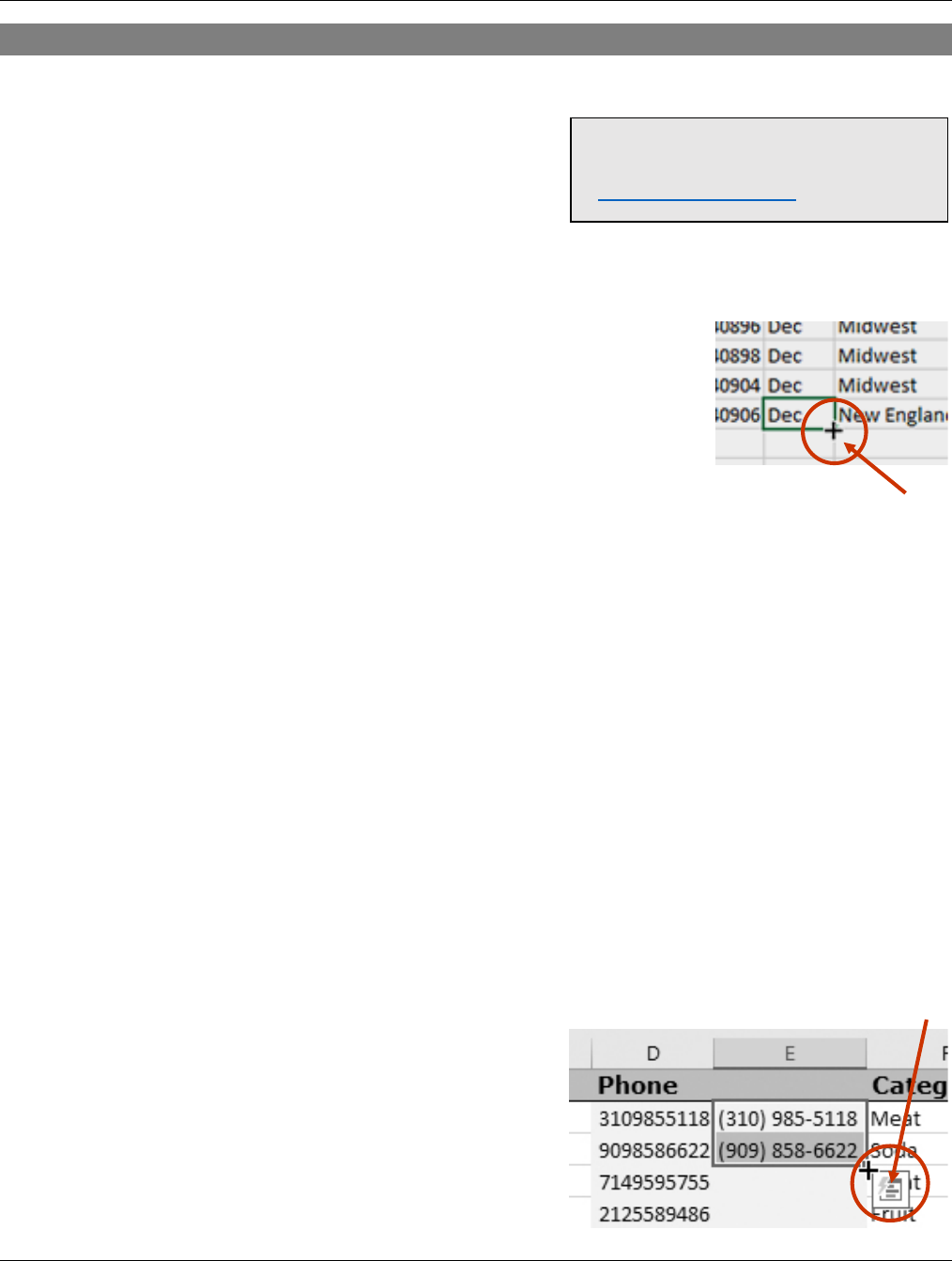
FLASH FILL SERIES
1. Place your cursor in an empty column to the right of the data that needs to be re-structured
(you may have to create this column).
2. Type the desired structure for the data and press
enter.
3. In the next cell down, again type the desired data
structure and press enter.
4. Highlight both cells together which maintain the
desired data structure.
Related Video
Auto Fill and Flash Fill

Excel ll – Fill Downs, Sorting, Functions, and More
6
5. Place your mouse on the Autofill Handle of the cursor.
6. Click and Drag down over numerous cells and let go.
7. Click on the Auto Fill Options button right next to the Autofill Handle and choose Flash Fill.
Excel ll – Fill Downs, Sorting, Functions, and More
7
SORTING
NOTE: Make sure row 1 in your spreadsheet or the first row in the table/range you wish to sort is
formatted as a header row. Sorts only work on contiguous rows in a range. Sorts will not work in a
range with empty rows or empty cells in the column you’re sorting.
BASIC SORTING – SINGLE COLUMN
1. Place your cursor in a column that you wish to sort its data.
2. In the Home tab, click on the Sort & Filter button and choose Sort A to Z.
NOTE: Depending on the column’s data type definition (Text, Number, Date, Etc.) it will sort from
smallest to largest (numbers) alphabetically for text, newest to oldest (dates).
SORT MULTIPLE COLUMNS
1. Place your cursor anywhere in a column heading
that you wish to sort its data.
2. Click on the Sort & Filter button and choose
Custom Sort…
3. Under Column, click on the Sort by drop-down list and choose which column you wish to sort.
4. Under Order, choose which order you wish to sort by.
5. Click on the Add Level button and in the Sort by drop-down and choose another column to
sort by.
6. Under Order, choose which order you wish to sort by.
7. Click on OK.
Your first column is sorted and the second column is sorted within the first sort.
SORT CUSTOM ORDER
1. Place your cursor anywhere in a column that you wish to sort its data.
2. Click on the Sort & Filter button and choose Custom Sort…
3. Under Column, click on the Sort by drop-down list and choose which column you wish to sort.
4. Under Order, choose Custom list…
5. In the List entries: build your custom list by typing one instance of each data type and
pressing enter between each one (list of how you want the data sorted).
You’ll end up with a custom data sort order.
6. Click on Add.
7. Click on OK and OK again.
Related Video
Sorting and Filtering
Excel ll – Fill Downs, Sorting, Functions, and More
8
FILTERING
Filtering is about showing only records that fit certain criteria.
NOTE: Make sure row 1 in your spreadsheet or the first row in the table/range you wish to sort is
formatted as header row.
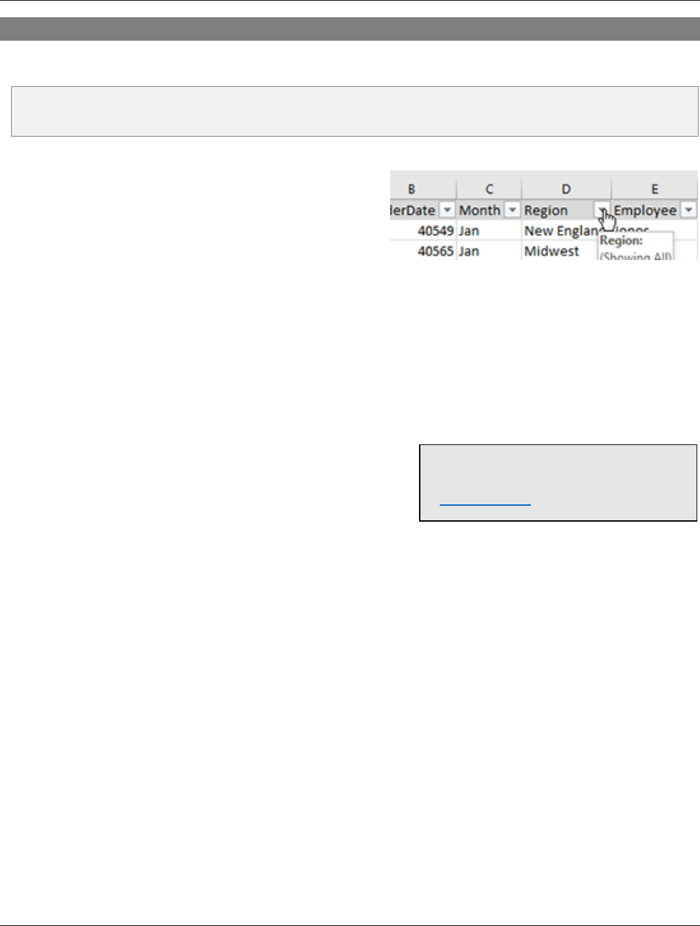
FILTERING BY VALUE
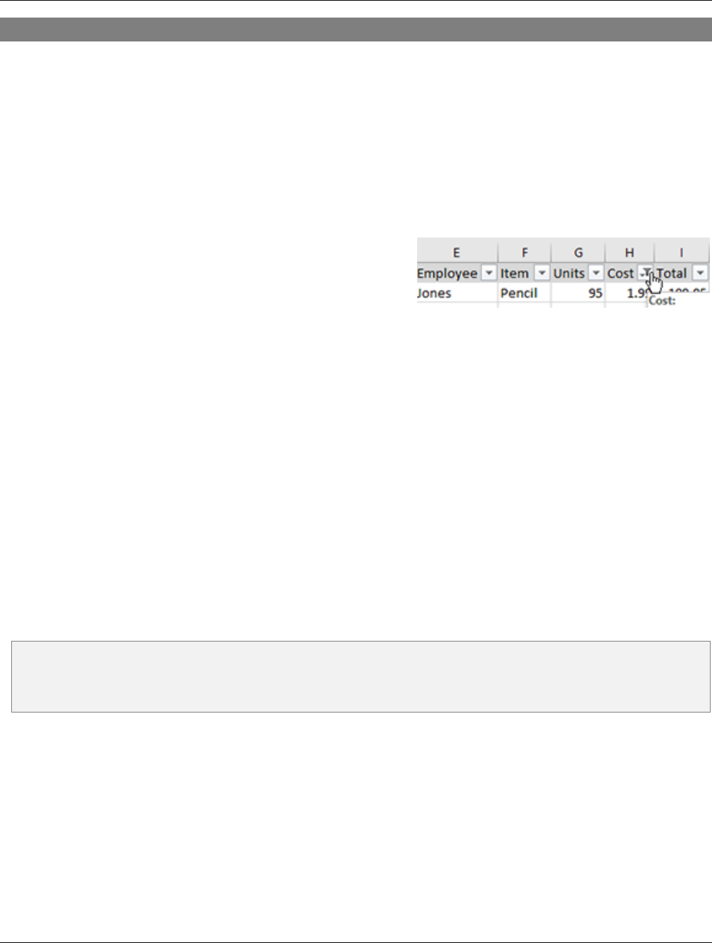
1. Click in a column heading you wish to filter.
2. Click on the Sort & Filter button and choose
Filter.
You will see Auto Filter down arrows in your header rows.
3. Click on the Filter button in the column you wish to filter.
4. Remove the check mark for Select All.
5. Place a check mark on the data type you wish to filter for.
6. Click on OK.
MULTIPLE FILTERS
1. Create a desired filter on a column (see above).
2. Click on the Filter button for another column you
wish to filter.
3. Choose the filter you wish to create.
You have filtered once for data criteria in the first step, and then within this same data,
added an additional filter.
Related Video
Filtering Data
Excel ll – Fill Downs, Sorting, Functions, and More
9
CONDITIONAL FILTERING
1. Click in a column you wish to filter.
2. Click on the Sort & Filter button and choose Filter.
You will see Auto Filter down arrows in your header row.
3. Click on the Filter button for a column which
maintains number values.
4. Point to Number Filters and choose Less Than Or Equal To…
5. Enter a value.
6. Click on OK.
Note: To clear your filter, click on the filter icon on the auto filter button for the column you have a
filter applied and choose Clear Filter From “column name”. To remove the auto filter feature from
your headings, click on the Sort & Filter button and choose Filter.
Excel ll – Fill Downs, Sorting, Functions, and More
10
BASIC FUNCTIONS AND FORMULA DEVELOPMENT
At its heart, Excel is a giant calculator. In fact, a simple way to think about Excel is to consider each
cell in a worksheet like an individual calculator. An Excel spreadsheet has millions of cells, which
means you have millions of individual calculators to work with. Not only that, but you can create
formulas that link different cells together (e.g. add the value in this cell to the value in that cell).
Interesting fact: up to 1,048,576 rows and 16,384 columns. Column width can be 255 characters.
FORMULA BASICS
All formulas begin with the = character. This alerts excel the
entry is a formula, not a value entered.
Example to Adding: =SUM(5,5) or (5+5) The resulting
cell value will be 10
Example to Subtraction: =SUM(a4-a3), Multiplication =SUM(a3*a4), Division =SUM(a3/a4)
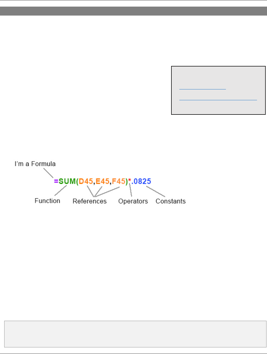
FORMULA SYNTAX
A formula can also contain any or all of the following: functions, references, operators, and constants.
Functions: The SUM Function allows you to do basic arithmetic within its parentheses.
References: D45 returns the value currently in cell D45, E45 returns the current value of cell E45, etc.
Operators: The * (asterisk) operator multiplies numbers.
Constants: Numbers or text values entered directly into a formula, such as .0825.
R
EFERENCING CELL RANGES IN FORMULAS
Referencing non-contiguous cells – A2,T66,L155,C5
Referencing a contiguous vertical range (range in a column) – C2:C54
Referencing a contiguous “table” range (rows and columns together) – C4:M276
Referencing multiple cells and or ranges - A2,T66,L155,C5,C4:M276
Note: Wherever your cursor is located in the sheet, the Formula Bar will show you it’s true
contents. This will confirm whether or not the value in the cell is a static value entered in the cell or
a value that is the result of a formula otherwise hiding in the cell.
Related Videos
Creating Formulas
Formulas and Cell Referencing

Excel ll – Fill Downs, Sorting, Functions, and More
11
COMMON FUNCTIONS
SUM
1. Place your cursor in cell K66 below the column of
units sold (number values).
Example: a column of number values in column
K which span from cells K3 to K65.
2. Type =SUM(K3:K65).
Where K3 is the beginning of the numbers to be
added and K65 is the final number to be added.
3. Press enter.
AVERAGE
=AVERAGE(cellref:cellref)
Returns the average of the numbers found in the cell range defined.
MIN
=MIN(cellref:cellref)
Returns the minimum value of the numbers found in the cell range defined.
MAX
=MAX(cellref:cellref)
Returns the maximum value of the numbers found in the cell range defined.
COUNTIF, COUNTIFS
=COUNTIF(cellref:cellref,”criteria”)
Returns the number of entries that comply with the defined criteria in the referenced
range.
=COUNTIFS(cellref:cellref,”criteria”, cellref:cellref,”criteria”, cellref:cellref,”criteria”)
Returns the number of entries that comply with each defined criteria in each referenced
range.
Related Videos
SUM and SUMIF formulas
AVERAGE Formula
COUNTIF Formula
COUNTIFS Formula
Excel ll – Fill Downs, Sorting, Functions, and More
12
FORMULAS - ABSOLUTE CELL REFERENCING
FORMULAS AND AUTOFILL
Consider the formula below which we could use to get the
product of two cells holding numeric values.
1. In L3 (Sub Total), type =SUM(i3*K3).
2. Autofill the above formula down the column it lives in.
Nicely enough the row reference number in the formula increases by one automatically
each time you fill down a row, again and again.
3. Under the Tax column cell M3, type =sum(L3*.0800) to get the tax amount of your subtotal.
a. Fill down to row 65.
NOTE - This feature allows us to autofill formulas that should change slightly relative to each
column or row they are found in.
FORMULAS WITH ABSOLUTE REFERENCING
Consider this formula which we could use to generate the taxable value on an item sold;
=sum(L3*.0800)
NOTE – We should rarely place numeric values in formulas. If we autofill the above formula;
=sum(L3*.0800), the result would be a Tax Column of possibly thousands of rows and thousands of
formulas – each one containing the value of .0800. However, the tax rate may change tomorrow.
1. Place the tax rate of .0825 in cell T10.
2. Now rewrite the above formula without referencing the tax rate value, reference the cell
which holds the tax rate value.
Example: =SUM(L3*T10)
(T10 being the cell you chose to hold your tax value)
Now if the tax rate changes you don’t have thousands of formulas to change – only the
value in cell T10.
3. Autofill this formula down the Tax Column.
You’ll notice a problem. The reference to T10 changes as you fill down to T11, T12, T13 and
so on. But your tax rate figure is sitting absolutely in cell T10.
4. Change the above formula to; =SUM(L3*T$10).
The dollar sign ($) will lock the row reference in the formula at 10. Now when you fill down
the row the reference of T10 will not increase by 1 with each row when filling down.
NOTE – Ultimately since the tax value will forever stay in cell T10, you’ll actually want to lock both
the column and row reference like this; =SUM(L3*$T$10).
Related Video
Absolute Cell Referencing
Excel ll – Fill Downs, Sorting, Functions, and More
13
PASTE SPECIAL
When looking at data in a excel sheet or cell you may simply see a value alone. However, that cell
may contain a value, visual formats, as well as a formula. With paste special you can choose which
one of these attributes you paste.
PASTING INDIVIDUAL ATTRIBUTES
1. Highlight a range of cells which maintain values, visual
formats (borders and shading, font, etc.), as well as a
formula.
2. Right-click on the highlighted range and choose Copy.
3. Right-click in the cell where you wish to paste.
4. Point to Paste Special and choose Paste Special.
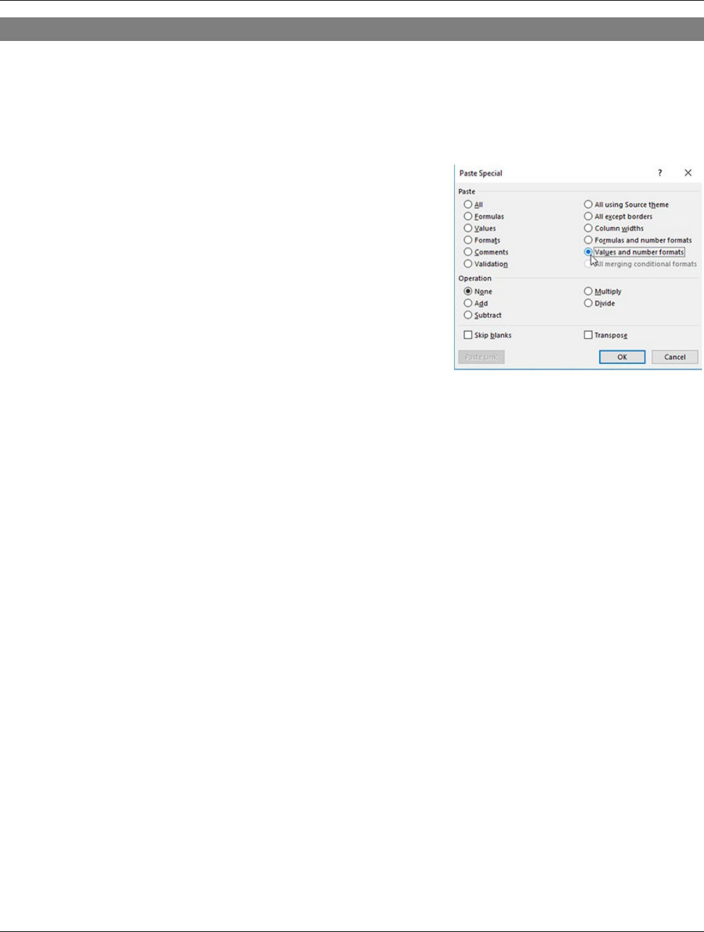
5. In the Paste Special window, choose from one of these:
FORMATS
Your resulting paste job has only pasted the visual formats.
VALUES
Your resulting paste job pastes only the values in the cells.
FORMULAS
Your resulting paste job paste job has only pasted the formulas.
VALUES AND NUMBER FORMATS
Your resulting paste job pastes the values and keeps the number formatting.
TRANSPOSE RANGE
Pastes the copied range, but switches what was rows to columns and vice versa.
COLUMN WIDTHS
1. Highlight a column which maintains a width you’d like to apply to other columns.
2. Right-click on the highlighted range and choose Copy.
3. Highlight the column you wish to replicate the column width to, right-click in the column,
point to Paste Special and choose Paste Special.
4. In the Paste Special window, choose Column widths.
5. Click on OK.
Your resulting paste job has replicated the column width.

Excel ll – Fill Downs, Sorting, Functions, and More
15
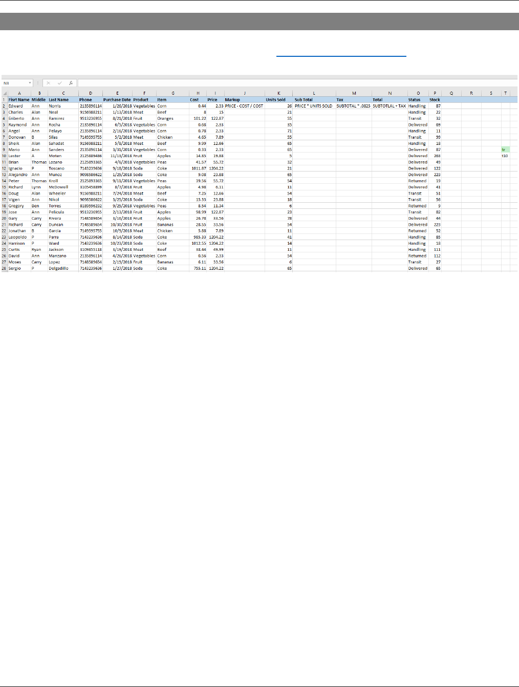
PRACTICE FORMULAS
Excel File = Example Spreadsheet.xlsm, ask techtraining@sbcusd.com for this file to
practice the following:
TOTAL UNITS SOLD
At cell location K66, total all the numbers above.
=SUM(K2:K65)
SUB TOTAL
At cell location L3, generate a sub total for the price for all units sold
=SUM(I3*K3)
COMPUTE TAX
At cell location M3, generate the tax amount
=SUM(L3*T$10) T10 holds your tax rate, the $ allows fill down to work without
changing 10
TOTAL
At cell location N3, generate the total
=SUM(L3,M3)
MARKUP
At cell location J3, determine markup percentage
=SUM(I3-H3)/H3
