EXCEL Introduction Class

CPA Info# 388 September 2020

Surviving

Excel

Lamar Smith and Hal Pepper

Designed for use in Advanced Got Farm Records… Now What? Workshop

This workshop is made possible, in part, through a Southern Risk

Management Grant supported by USDA/NIFA under Award Number 2018-

70027-28585.

Surviving Excel

Lamar Smith

Consultant

Hal Pepper

University of Tennessee Extension Specialist

Excel Class 1

1. Introduction 1

2. Starting Excel 1

3. Moving Around Excel 1

4. Entering Formulas 4

5. Saving the Work 9

Excel Class 2

1. Introduction and Review 10

2. Inserting and Deleting Rows, Columns and Cells 10

3. AutoFill 11

4. Formatting Cells 11

5. Print Preview 17

Excel Class 3

1. Comma Separated Value Files 19

2. Creating an Estimating Tool 23

3. VLOOKUP Function 24

EXCEL Class 1

1. Introduction

Old-fashioned spreadsheets were used by accounting types. In its day, a

spreadsheet was a multi-columned paper that allowed managers to view

accounting information “spread” out into multiple columns that represented

accounts. This allowed for accurate decision making. Excel was born from a

desire to produce an electronic version that could do math automatically. It has

become much, much more than that.

2. Starting Excel

Excel is started by clicking on the Excel Icon, or depending on your version,

through the Start, Programs menus.

Select Blank Workbook to open a blank workbook.

Menus across the top may include File, Home, Insert, Page Layout, Draw, …

Menus will vary according to the version of Excel you have.

Toolbars are located under the menus.

All the toolbars can be customized to meet your needs. But you can’t know what

your needs are until you know something about what Excel can do for you.

3. Moving Around Excel

Cells: Cells are the rectangles all over the screen. Each one is a place holder

for information.

Cell Address: Column and Row designation. A cell in column C on row 3 has

the cell address of C3. The cell address is displayed in the top left-hand corner

of the spreadsheet.

If you know the address of the cell you want to move to, you can move directly to

that cell by using the “Go to…” function. It is located on the Home menu under

Find & Select. If you can remember the “G” in “Go to” then you could use the

hot key (CTRL)+G.

Cells can hold numbers, dates, times, text, or formulas. To begin with, we will

just focus on entering numbers and formulas. Once we understand how that

works, then we will expand into some other types of information like dates and

text.

Active Cell: The active cell has a box around it. There are several ways to move

between cells.

Mouse: Click on the cell desired.

Arrow Keys: Scroll to the cell desired.

Scroll lock on – window pans

Scroll lock off – active cell changes

The box will move as the arrow keys, the return key or a mouse click activates

another cell.

Some important terms:

Worksheet or Spreadsheet: A single grid of cells. The name of the worksheet

or spreadsheet is the name on the tab at the bottom.

Workbook: A series of worksheets or spreadsheets in one computer file. The

name of the workbook is the name of the file.

Formula Bar: Located across the top of the spreadsheet. It is a place to enter

the formula to be calculated.

Exercise 1 - Formulas

Open the file: Excel Class Tenn.xlsx.

Click on the Formulas worksheet tab. Starting in cell A1, enter a number

followed by the Enter key. Depending on how Excel is configured, the

active cell will now be A2, B1, or still on A1. Just enter some numbers into

Excel to get a feel for how numbers are accepted. You can use the Enter

key, Tab key or use a Cursor (Arrow) key to input the value.

Deleting: The contents of a cell can be deleted by selecting the cell and

touching the delete key. This action empties the contents of the cell. It does not

remove the cell from the spreadsheet or change the appearance in terms of font,

color, etc.

Exercise 2 - Formulas

Make sure you are working in the Formulas worksheet tab. Highlight a

cell with a value. Press the delete key. The value stored is removed.

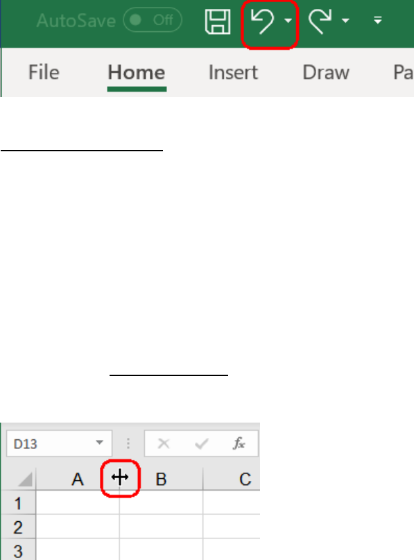
Undo: Any action can be undone by using the “Undo” feature or Control

(CTRL)+Z.

Exercise 3 - Formulas

Make sure you are working in the Formulas worksheet tab. Click the

Undo icon at the top or use (CTRL)+Z. The information deleted in

exercise 2 is restored.

Adjusting Column and Row Size: At the top of each column is a column label.

It is gray with the letter designator of the column in it. At the left of each row is a

row label. It is gray with the number designator in it.

The size of the column or row can be adjusted to provide the necessary space

for the value by hovering the mouse pointer over the line which divides the

column or row in the label area. The pointer will change to a bar with arrows

pointing out from the bar. The bar is vertical for the columns and horizontal for

the rows.

Vertical bar shown above for a column.

Once the pointer changes, left click and hold to drag the row or column to the

size desired.

Clearing Whole Rows or Columns

A whole row or column can be highlighted by clicking on the label area of the

row or column desired. Once highlighted, press the delete key to remove the

information. This process only clears the values. It does not remove the row or

column from the spreadsheet.

Exercise 4 - Formulas

Make sure you are working in the Formulas worksheet. tab Adjust the

row height and column width to experience how the adjustment can be

made.

4. Entering Formulas

One of the main uses of Excel is to design the sheet so it will calculate values

automatically. The most simple formula that you can enter is: =[cell address].

Exercise 5 - Formulas

Make sure you are working in the Formulas worksheet tab. Enter

numbers in cells A1 through A4 and B1 through B4. You may want to

enter simple numbers on which you can perform simple math in your

head. Now, in cell E1, enter “=A1” followed by the Enter key. Whatever

value is stored in cell A1 now appears in cell E1. Also, notice the results

in cell E1 as you change the value in cell A1.

Basic Math Formulas: Excel is a math program. It will do basic math functions

and much, much more. We will start with the math functions add, subtract,

multiply, and divide. These are the building blocks of all mathematical functions.

Excel uses some symbols for these math functions that you might not be used to

using. These four types of math functions are represented in formulas as:

Addition – plus sign (+)

Subtraction – minus sign (-)

Multiplication – asterisk (*)

[above 9 on number pad or shift+8 on keyboard]

Division – slash (/)

[above 8 on number pad or next to right shift on keyboard]

Using these symbols we can write formulas that perform math functions for us.

The one trick you need to remember is that the equals sign goes at the

beginning, not the end. The equals sign tells Excel that you are entering a

formula and that you want Excel to calculate what follows.

Exercise 6 - Formulas

Make sure you are working in the Formulas worksheet tab.

In cell C1, enter “=A1+B1” followed by the Enter key.

In cell C2, enter “=A2-B2” followed by the Enter key.

In cell C3, enter “=A3*B3” followed by the Enter key.

(Select cells using arrows.)

In cell C4, enter “=A4/B4” followed by the Enter key.

(Select cells using mouse.)

Notice the results in column C. Change the values in columns A and B

and notice how the results update.

Order of Operation: You should also be aware that the order of operation

holds true in Excel. Remember the rule we learned in school that to evaluate a

mathematical expression, first multiply, then divide, next add and finally subtract.

Use parentheses to group math operations that should be performed first.

Exercise 7 – Operation Order

Make sure you are working in the Operation Order worksheet tab. The

following information has been entered in the spreadsheet under the

worksheet tab “Operation Order.”

A2 = 3 ; B2 = 7 ; C2 = 20

A2 represents the number of people in one group.

B2 represents the number of people in a second group.

C2 represents the fee to be collected.

The mathematical expression =A2+B2*C2, or 3+7*20 will produce a result

of 143 because multiply and divide occur first in the order of operation.

First 7 x 20 = 140, then add 3 = 143.

But, if we want to first add the number of people in the two groups and

then multiply the result by the fee, we can place parentheses around the

expression A2+B2. The formula would be expressed in cell D2 like this:

=(A2+B2)*C2

This says first add 3+7 for a sum of 10, then multiply by 20 for a total of

200.

Relative Cell Reference: Instead of having to enter each individual formula into

each individual cell, Excel copies formulas into cells semi-intelligently. When the

formula is copied down the spreadsheet, the formula is changed by Excel to

reference the correct set of cells relative to the position of the new formula

location.

Exercise 8 – Formulas

Make sure you are working in the Formulas worksheet tab. In the

Formulas worksheet tab, highlight column C only and press delete.

For each row (2, 3, 4, etc.), I want each cell in column C to be the result

of adding the value in column A to column B.

I could manually enter the formula over and over in each cell of column C,

changing the row reference for each row, but there is an easier way.

Make cell C2 the active cell. In cell C2 enter the formula =A2+B2. Press

Enter and move the active cell back to cell C2. (You’ll notice the active

cell has a box around it as we discussed earlier.) In the lower, right hand

corner of the box is a green square. This is a handle. Notice how your

cursor will change from a large white cross to a small black cross when

you touch the handle. So, hover the cursor over the handle so that the

cursor is a small black cross, click and hold the left mouse button, then

drag the box down to cover cells C2 through C4. Release to see the new

answers in column C.

Relative Cell Reference gives us the ability to copy formulas down or across the

spreadsheet and have the formula automatically updated for the cell reference.

If you copy down, the row numbers are indexed. If you copy across, the

columns are indexed. But you can’t do both at the same time. That would just

be too confusing for Excel.

A word of caution. You can make a mistake right here if you’re not careful. So, if

you attempt to drag the formula in our example from C1 to D1, your formula will

not mean much because it would become a formula that takes the answer and

adds to it again one of the numbers used to produce the answer. There are

times when relative cell reference will not work for you and there is another way

to handle those situations. We’ll come to that in the next exercise. First we need

to talk about functions.

Sum Function: The makers of Excel knew that we would be doing a lot of

totaling long lists of numbers. If we had a list of 6000 values and wanted to total

the whole list, that would be quite a long formula (=A1+A2+A3+A4… all the way

to A6000). We have a way to short cut that process. One way of making this

statement would be to add up all the numbers from A1 to A6000. The “SUM”

function does exactly that.

Look for an icon on the tool bar that looks like the Greek symbol “Sigma”. It

looks like a letter M laying on it’s left side. Like this: “ Σ “ This is the Sum button.

Exercise 9 – Functions

Make sure you are working in the Functions worksheet tab. The

Functions worksheet shows hypothetical vegetable production in acres for

each county for each year under consideration. We need totals for each

county and totals for each year.

Make cell F3 active.

Click the SUM button on the tool bar. Notice the blinking line around the

range of cells that will be totaled. Cells B3, C3, D3 and E3 should be

blinking.

Press Enter and the formula will display the results.

Make cell F3 active and copy down to cell F13 using the handle of the

active cell. We now have totals for each county.

Now make cell B15 active.

Click the SUM button on the tool bar. The blinking line encompasses the

cells from B2 to B14. By clicking and dragging the mouse over the range

of cells I want to sum (B3 to B13), the formula is updated to only sum the

range I desire.

Press Enter and the formula will display the results.

Make cell B15 active and copy over to cell F15 using the handle of the

active cell. We now have totals for each year for all counties and a grand

total for all.

Absolute Cell Reference: Relative Cell Reference says that as the formula is

copied down or across the sheet the cell addresses will be indexed in the same

direction either down rows or across columns. There are occasions when you

will want to have a formula that does not index down or across. Exercise 10

demonstrates this.

Exercise 10 --Functions

Make sure you are working in the Functions worksheet tab. I want to find

out the annual percentage of total acres in vegetables produced over a

four-year time period by year. In other words, over the time period, what

was the percentage of total acres for each year?

In cell B17 enter =B15/F15. This divides the annual total by the grand

total for a percentage.

Make cell B17 active and drag copy across to cell E17 by using the

handle of the active box.

The error “#DIV/0!” means you are trying to divide by 0. You’ll remember

from our school math that no number can be divided by 0. It’s impossible.

To correct this problem, we need to change part of our formula to use

“absolute cell reference”. In a formula, when a row or column is preceded

by a dollar sign ($), then the row or column value will not change as you

copy it from cell to cell.

So go back to cell B17.

Press the F2 key to allow you to edit the formula or double click on the

cell.

Now move the cursor to just before the F and place a dollar sign ($) there.

Then, move to just after the F and put another dollar sign ($) there. This

locks the cell reference.

Copy the formula by dragging across to cell E17 and this time the proper

answers appear.

Copy and Paste: Now that you understand about “relative cell reference” and

“absolute cell reference”, you can now see how cut and paste can work for you

when copying information. Copy and paste (just like in Word) will copy values or

formulas according to the rules of relative and absolute cell reference.

Exercise 11 --Formulas

Make sure you are working in the Formulas worksheet tab. On the

Formulas worksheet, highlight cells A2 and B2.

Once highlighted, the cells can be copied as follows:

Use Edit menu, then Copy, (or)

(CTRL)+C, (or)

Right clicking on the highlighted cells and selecting “Copy” with a

left click.

Move the active cell to A9 and paste the cells as follows:

Use Edit menu, then Paste (or)

(CTRL)+V (or)

Right click on cell A9, then left click on Paste.

Move the active cell to C2 and copy as described above.

Move the active cell to C9 and paste as describe above.

The formula was copied and pasted, and the formula cell address was

updated to continue to add the columns as you structured them.

Paste Special: There are occasions that you do not want a formula to be

pasted. For example, you may want the result pasted instead of the formula. In

this case, you may want to use “Paste Special.”

Exercise 12 --Formulas

Make sure you are working in the Formulas worksheet tab. On the

Formulas worksheet, make cell C3 the active cell and copy the cell

(CTRL)+C.

Move the active cell to cell F15 (any unrelated cell will do).

To use Paste Special, use 1 of the 2 following methods:

1. Select the Edit or Home menu and under Paste, choose Paste

Special (or)

2. While pointing to the destination cell, right click and then select

Paste Special.

Select “Values” from the display of Paste choices and select Okay.

Notice that the contents of the cell pasted is not a formula. Instead, the

contents of the cell pasted is the result of the formula.

Paste Special is handy when you don’t want the user of the spreadsheet to be

able to adjust the displayed values in a cell. For example, you may not want a

particular cell to be linked to other cells with formulas. With Paste Special the

results of a formula are pasted to a cell instead of the formula itself.

5. Saving the Work

To save the workbook select File, then Save. If the workbook has never been

saved before, Excel will require a file name. If it has been saved previously, the

old copy will be over written.

The icon on the toolbar (the one that looks like a disk) serves the same purpose.

There are occasions when you might like to take an existing workbook and save

a new copy with a different name. In this case, select File, then Save As. You

will be prompted for a new file name before the saving will be executed. There

is not a tool bar icon for this feature.

EXCEL Class 2

1. Introduction and Review

We have learned about cells, active cells, worksheets, workbooks, relative cell

reference and absolute cell reference.

We learned about how to enter numbers and formulas into cells. We know that

formulas all start with an equal sign. Excel uses 4 symbols to perform the basic

functions of math: Addition (+), Subtraction (-), Multiplication (*) and Division (/).

This session will deal with the formatting of the information into a presentable

format. All the numbers in the spreadsheet might be valuable but without some

text to describe what the numbers represent, the spreadsheet would be

meaningless.

2. Inserting and Deleting Rows, Columns, and Cells

Right click on a row or column to view the menu. Click on insert to add a row

between two rows or a column between two columns. If you highlight a row, you

will add a row. If you highlight a column, you will add a column.

Delete key vs Right Click and select delete

Exercise 1 – Inserting/Deleting

Open the file: Excel Class Tenn.xlsx.

Click on the Insert & Delete worksheet tab. Select cell B2 and press the

delete key. This removes the value from cell B2 only and leaves the cell.

It leaves all other values in their place.

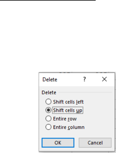
Click on cell C2, then right click while pointing to cell C2. Select

“Delete”. You will be asked to choose the direction that you want to shift

the cells.

This is a destructive delete. It is removing the cell from the spreadsheet

and shifting the cells around it to take its place. The question Excel wants

answered is “Do you want to shift the cells up or over from the side?”

Click on cell C2, then right click while pointing to cell C2. Select “Insert”.

This process can be reversed and cells inserted. Excel will again ask

which way to shift the cells.

Select a row or a column for insertion or deletion by selecting the whole

row or column, right click for the short cut menu, then choose “Insert” or

“Delete.”

Be careful how you delete information. You could be deleting a cell and not just

a value. You are able to use “Undo” to restore the cell.

3. AutoFill

Just like cells can hold numbers, cells can also hold text, dates or time values.

The numbers, text, dates and times can be formatted to suit the appearance you

desire.

Exercise 2 – Auto Fill

In Cell A10 of the Insert and Delete worksheet tab, enter “Jan”. Then

grab the handle of the cell and drag down to copy the names of the

months into the adjacent cells. The same can be done with the days of

the week.

You can create your own number series as well by entering the first two

values, highlighting both cells, and dragging the handle in the direction

desired.

4. Formatting Cells

Just like cells can hold numbers, cells can also hold text, dates, or time values.

The numbers, text, or dates and times can be formatted to suit the appearance

you desire.

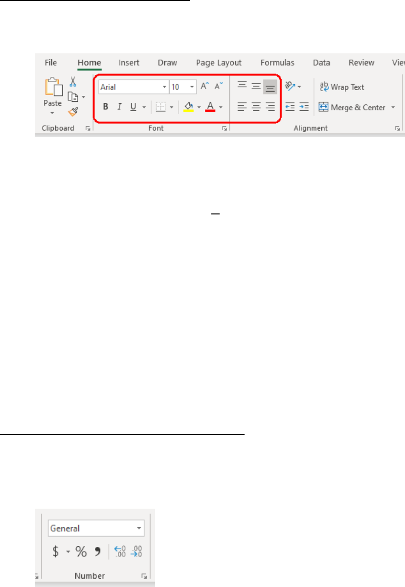
Many of the format changes can be done right from the toolbar at the top of your

screen. The following exercise illustrates the use of these toolbar features to

change the appearance of the cell.

Exercise 3 – Formatting from toolbar

Click on the Formats worksheet tab. Cell A1 does not have any special

formatting applied. It bears the default format. Make the following

formatting changes using the toolbar. We’ll leave A2 for comparison.

In cell A3 click on Bold B

In cell A4 click on Italics I

In cell A5 click on Underline U

In cell A6 click on Left Justification

In cell A7 click on Center

In cell A8 click on Right Justification

In cell A9 change the Font size

In cell A10 change the Font style

In cell A11 change the Background Color

In cell A12 change the Font Color

These buttons did nothing to change the value or the way the value is stored in

Excel. There are a few other buttons along this toolbar that pertain to the format

of the value. These buttons are demonstrated in the following exercise.

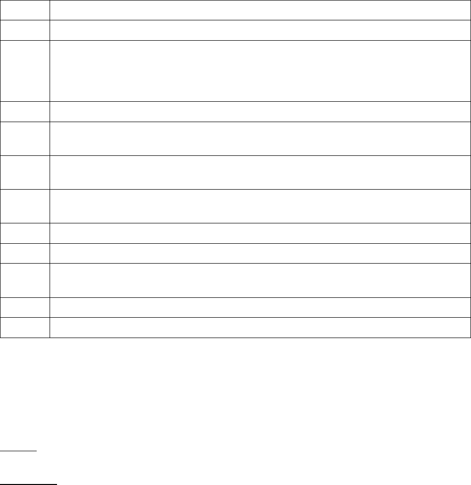
Exercise 4 – Formatting Numbers from Toolbar

Click on the Formats worksheet tab. Cell C2 does not have any special

formatting applied. Enter the number 5000 and select enter. Make cell

C2 the active cell. Then select each of the following buttons to see the

change on the value.

Currency

Percentage

Comma

Decimal Increase

Decimal Decrease

Advanced formatting: To change the format of a single cell, group of cells,

whole row, or column, first highlight the range of cells to be formatted. Right click

on the range. From the short cut menu, select “Format cells…” The Format

Cells control panel appears with 6 different tabs to control the appearance of the

cells. We’re going to cover the following tabs in this session: Number, Alignment,

Font, Border, Patterns.

Number: Well, they had to call it something and Excel is a number program, but

what this tab really does is allow you to define what type of information will be

contained in the cell. In the next exercise, we will format different cells using the

number tab.

Exercise 5 – “Format Cells…” from Short Cut Menu

Click on the Formats worksheet tab. Column B does not have any

special formatting applied. Enter the number 100,000 in cell B2. Highlight

cell B2 and copy down to cell B5. We’ll leave cell B2 formatted as

General as a point of comparison. Make cell B3 the active cell. Right click

on cell B3 and select “Format Cells…” from the short cut menu. If the

“Numbers” tab is not selected, then click on it to display the Numbers

options. Table 1 outlines the settings available for formatting the value of

a cell.

Table 1. Settings Available for Formatting the Value of a Cell

Cell

Format

General – Let Excel try to figure it out. (default setting)

B3 Number – Always treat the value as a number. No letters are expected.

Number of decimal places to show. (This rounds the display, not the value.)

Choose whether to use a comma to separate at each thousands break.

Choose how to display negative numbers.

Currency – Money. Same as Number but adds a symbol for currency.

B5 Accounting – Money but aligned with “$” sign to the far left. Accountants use

parenthesis to indicate negative values.

B6 Date – Choose how to express the date, such as MM/DD/YY or DD/MM/YY or

as a 4 digit year. Choose whether to spell the month out.

B7 Time – Choose how to express the time in hours and minutes, as a 12-hour

clock or 24-hour clock

Percentage – Automatically format the value into a percentage.

Fractions – Display and calculate fractional values

B10 Scientific Notation – A format used by mathematicians to work with extremely

large numbers.

B11

Text – Information such as words or alpha characters.

B12

Special – Zip codes and SSN formats.

Alignment: The next tab of the Format Cells Control Box is “Alignment.” This

does just what it sounds like. It deals with the positioning of the information in

the cell and on the spreadsheet. The upper left area of the panel controls how

the value will be positioned in the cell horizontally and vertically. If left on

“General” the we’re leaving Excel to try to guess which way is best.

Indent: The indent control allows information to be indented in the cell to form a

sub list of main points.

Horizontal: This controls the positioning of the information horizontally.

Information can be:

• General, (Let Excel figure it out), Left, Center, Right, Fill, Justify, and

Center Across Selection. Left, Center, and Right do just what they say

they will do (i.e. Left puts the information to the left in the cell and Right

puts the information to the right in the cell.) You’ll use these frequently.

• Fill is interesting. It repeats the information as many times as is

necessary to fill the cell. (I haven’t found a use for this, yet.)

• Justify pads spaces between words to attempt to even the margins of the

words in the cell. (Don’t expect the results you get in Word.)

• Center Across Selection: This is a handy tool. This selection centers the

information in the cells that have been selected. Great for header

information at the top of a chart.

Exercise 6 – Formatting

Click on the Formats worksheet tab. In cell A1 type the following:

“Formatting Styles” and press enter. Now highlight cells A1 and B1. On

the “Alignment” tab select “Center Across Selection” in the Horizontal

drop down list and click on “Okay”.

Now the information which is really in cell A1 is displayed across the area

of cells A1 and B1. If any modifications are to be done to the text, they

must be done in cell A1. If new information is typed in cell B1, then the

text will not display as desired.

An example of this type of formatting is found on the Functions

worksheet tab in row A. Notice that the information is located in B1, but

displayed and centered from B1 to H1.

Vertical: The vertical control works similar to the horizontal control, but will

display differently due to the vertical orientation.

Text Control: This area has 3 check boxes to turn features on and off for the cell.

Wrap Text just allows the text to wrap automatically from one line to the next.

Note: A carriage return cannot be used in a cell. So if Wrap Text is on,

don’t expect to be able to display separate paragraphs of information.

Shrink to Fit is handy for allowing Excel to automatically choose a font that will

allow the text to fit in the cell when otherwise it would run off into the next cell.

Exercise 7 – Shrink to Fit Formatting

Click on the Formats worksheet tab. Look at column E. Due to the length

of the text fields, the names are overflowing into column F.

Highlight from E2 to E31. Select “Format Cells..” from the short cut menu.

On the “Alignment” tab select “Shrink to Fit”. Click on “Okay.” Notice how

the various names do not over flow into column F now.

Merge Cells allows the user to highlight a range of cells and force the range to

be considered as one cell by selecting “merge cells. I would suggest using

extreme caution when merging cells. There are times when there is simply no

other way to accomplish what is intended but to merge the cells. But, when

there are merged cells on a spreadsheet, you must be extra careful when

deleting rows or columns.

To see an example of merged cells and vertical text look at the array of

information in cells K1 through K4. Cells K1 to K4 were highlighted, then

merged. When the Text Control box was activated, the orientation for the text

was set for 90 degrees.

Text can also be stacked vertically by selecting the box that illustrates vertically

stacked text.

Font: The next tab over is Font. The font is the look of the letters and numbers.

In this tab the font can be selected as well as the style and size. Style in this

case refers to whether the font is bold, italics, or both. If you need to underline

the characters, there is a drop down box to chose the different styles of

underlining.

The size is easy to use. The bigger the number, the bigger the character.

Some other features are available here, such as the color of the font,

strikethrough (which means it puts a line through the text like this), superscript

(which means the characters are above the normal position like

this

), and

subscript (which means the character is below the normal position like

this

The normal check box will return the cell to the default settings and over ride the

special settings that were previously applied.

The default settings for the font is made in the following location. Click on Tools,

Options, General tab. Just below the middle of this tab is a place labeled

“Standard Font.” The font name and size are entered here to set the default font.

Borders: The next tab is the Borders tab. It is pretty simple and straight forward.

One the right hand side there are several different styles of lines to choose from

and the color is in a drop down box below. Once the style and color are

selected, click on the buttons that show the position of the border you need.

Buttons at the top remove borders, go all the way around the edge, and another

crosses them through the middle.

Patterns: The next tab is the Patterns tab. It is also very simple and straight

forward. At the top you are picking the background color of the cell and at the

bottom you can pick a pattern to hash the background. My advice concerning

patterns is that they make the cell values very hard to read unless the font is

very large and/or bold.

Protection: The Protection tab will not be covered in this class. It involves a

process where cells can be locked so that the user cannot change the values or

formulas. But it’s more complicated than simply checking or un-checking the

box on this tab.

5. Print Preview

Print Preview is a very helpful tool if you’re going to be printing the results of

your work. This tool allows you to view how the printed results will look when

sent to the printer. With the sheet highlighted, click on the File menu, then Print

to view a preview of the print version of the worksheet.

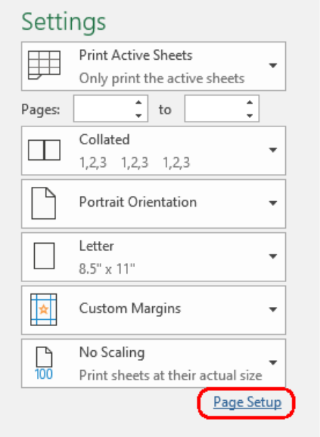
Under Settings you have control of how the document prints including Portrait or

Landscape Orientation, Paper size, margins, and scaling.

At the bottom of these setting is a link to Page Setup.

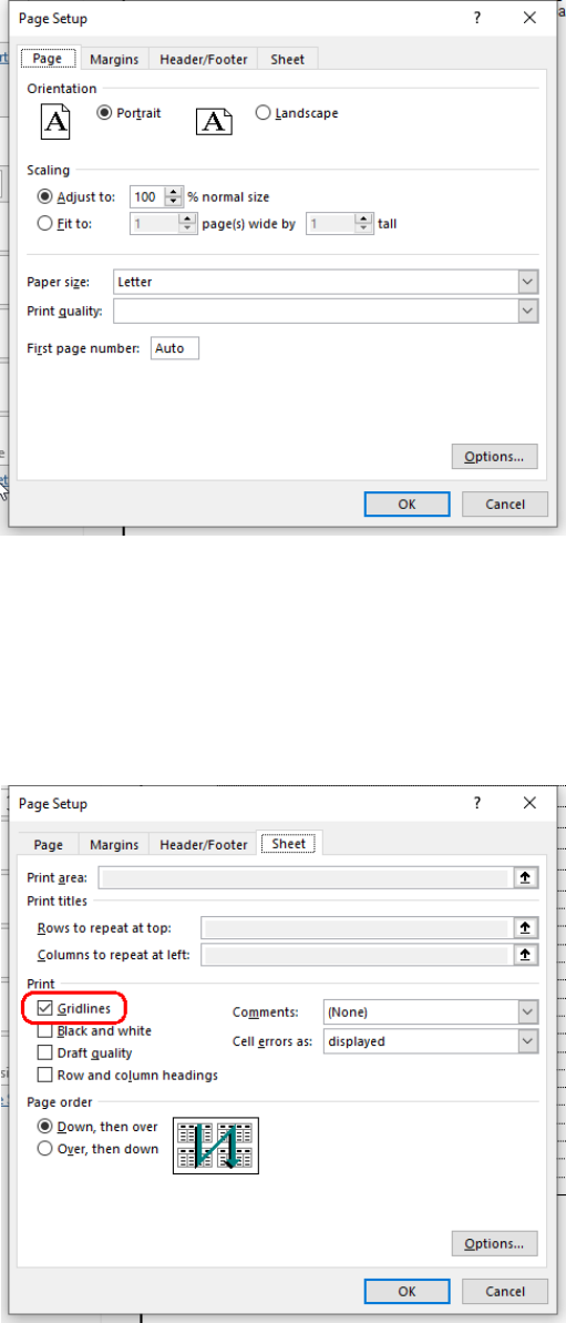
The Page Setup link opens many options to adjust how the page will print.

Each tab provides many options which control the printed appearance.

The margins of the printed page can be adjusted on the Margins tab. A Header

or Footer can be set for the page on the Header/Footer tab. You can set

gridlines to print on the Sheet tab.

EXCEL Class 3

1. Comma Separated Value Files

A Comma Separated Value (CSV) file is a text file organized in a consistent

order with each value separated (or delimited) by a comma. Each line or row in

the file is one record in the list. The first row of the file is usually a header row. A

header row defines the contents of the file.

Example:

FirstName,LastName,Address,City,State

Bryan,Gibson,105 Oak Street,Nashville,TN

John,Harris,2518 Elm Drive,Murfreesboro,TN

Gary,Smith,3840 Winona Drive,Tullahoma,TN

Often data is exported from other systems such as QuickBooks, Square, or a

bank as a Comma Separated Value file. This type of file can be named as a .txt

file but most often as a .csv file.

When the file is a properly formatted .csv file, Excel will open the file without any

effort from you. The file will appear as an Excel spreadsheet. You may have to

save the file as a .xlsx file depending on what you do to the contents of the file.

Excel also offers an import function for CSV files when they are not named as

a .csv file or are formatted slightly differently.

Importing a CSV file manually.

You’ll need to know from the source of the data how the file is formatted.

• Does the file have a header row?

• What delimiter was used to separate the values? (i.e. comma, tab,

semicolon, space, slash)

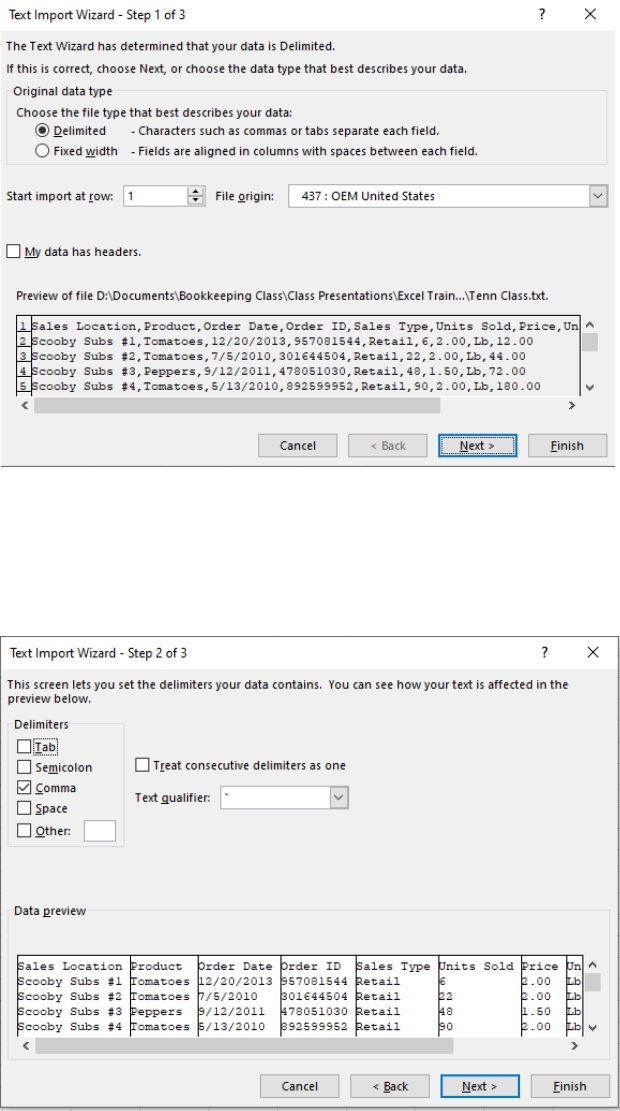
Using Excel, open the file Tenn Sales.txt and a Text Import Wizard box appears.

Step 1

Select Delimited or Fixed Width.

Indicate if there is a header row.

Select Next.

Step 2

Select Delimiter type

Select Next

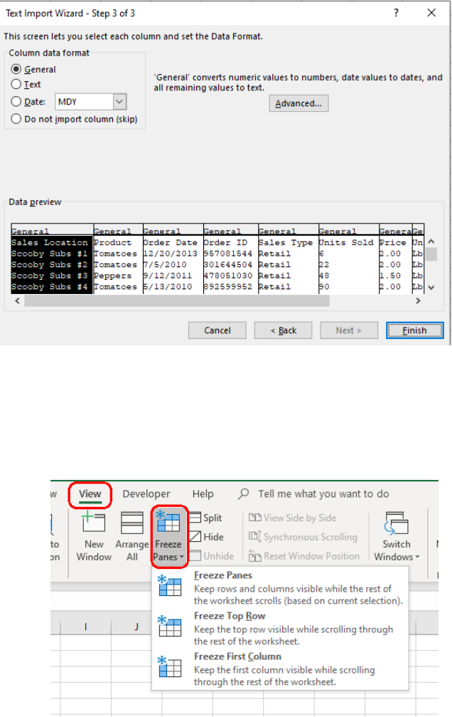
Step 3

Select Data Format (rarely needed)

Select Finish

Excel has imported the data into a spreadsheet format. We need to do some

formatting to make the data usable. We will go through the following

adjustments.

Freeze rows or columns

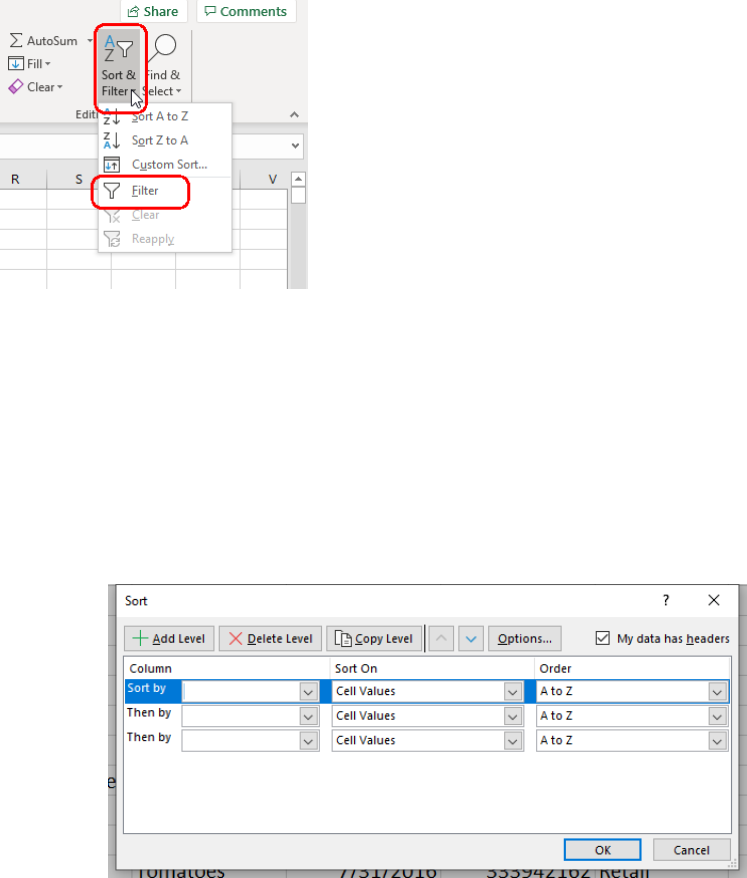
Set Filter on header row

With the filter in place, now we can sort and limit what data we want to view.

Rows can also be reordered from A to Z, Z to A, Number columns will sort

largest to smallest or smallest to largest. Date columns will sort oldest to newest

or newest to oldest.

Custom Sort

The sort feature in the filter is limited. You can only have a single column sorted.

There are times when a more complex order is required. By using the Custom

Sort (also found on the Data tab, Sort) multiple columns can be sorted by

column priority.

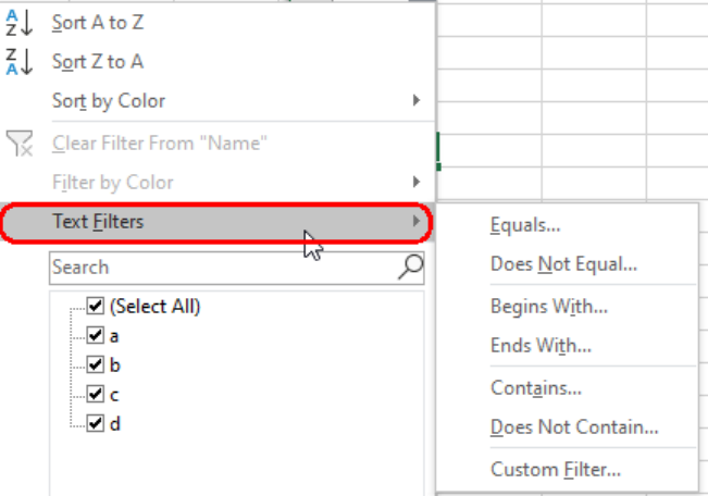
Filter by Text

By clicking on the drop down arrow for the filter of any header label, you can

filter by text. Searches include Equals, Does Not Equal, Contains and many

others.

Summing a filtered column

The sum() function will not update the total when the rows are filtered. To get a

filtered total, use the Subtotal() function.

Subtotal function. =subtotal(function_number,range)

The sum command for the subtotal function is 9. The subtotal function will limit

what rows are in consideration based on the view of the filter.

We’ll enter the following formula in cell I5003.

=SUBTOTAL(9,I2:I5001)

As we change the filtered results the sum will update to reflect the filtered total.

2. Creating an Estimating Tool

The spreadsheet Tomato Planner.xlsx contains a Planner tab for planning and

tabs for inputs labeled Plants, Plant_Starter, Potassium Nitrate, Black Plastic

and Drip Line. Each tab for inputs contains the cost information for these

required items.

We’ll use the following functions:

=AVERAGE(number1,…)

Returns the mathematical average of the range of numbers selected.

=ROUND(number, num_digits)

Rounds the number selected to the number of places indicated in the

num_digit field.

=ROUNDUP(number,num_digits)

Rounds the number up to the next value to the number of places

indicated in the num_digit field.

=MIN(number1,…)

Returns the minimum value

=COUNT(value1,…)

Returns the number of cells containing numbers.

Specific functions in the example spreadsheet Tomato Planner.xlsx we now

want to consider are ROUNDUP and a formula using SUM, MIN and COUNT to

average numbers where the lowest value is removed.

We will use ROUNDUP to determine the quantity of an item to be purchased

with a minimum increment requirement. (Example: Black Plastic is sold in 4000

foot rolls.)

=ROUNDUP(B13/Plants!B2,0)

The ROUNDUP() function is used because vendors sell in various

minimum increments. This will return the minimum purchase needed to

meet the volume required.

Average without lowest value:

=(SUM(C4:C7)-MIN(C4:C7))/(COUNT(C4:C7)-1)

When determining an average, some choose to eliminate the lowest value so

that the final result is not grossly understated. This nested series of functions will:

1. Sum all the values.

2. Subtract the lowest value.

3. Divide the new sum by the count of value less 1 (to account for the

removed lowest value).

3. VLOOKUP Function

To demonstrate the VLOOKUP function, we’ll open the Excel Class Tenn.xlsx

file. We’ll use the VLOOKUP and Data tabs.

The VLOOKUP function will find a matching value in an array and return a value

in the same column. The syntax is:

=VLOOKUP(lookup_value,table_array,column_index_num,[range_lookup])

lookup_value: The value to be found in the array.table_array: Where the

information is to be found.

column_index_num: The column where the value to be returned is

located in the array.

Note: VLOOKUP will only search in the 1

column of the array.

range_lookup: true or false are the possible values.

True is an approximate match (the search column in the array

must be in sorted in descending order).

False is an exact match.

In cell E2, we’ll put the following:

=VLOOKUP(B2,Emp,4,FALSE)

How to use an ampersand:

The ampersand (&) will join embedded text in a string of functions. For example,

we’ll use VLOOKUP to find the last name and the first name of the employee

and embed a comma after the last name as shown in this series of functions:

=VLOOKUP(B2,Emp,3,FALSE)&", "&VLOOKUP(B2,Emp,2,FALSE)