

Sports are a popular topic for course projects – usually involving
details of some specific sport and statistical analysis of data.
In this lecture we imagine some non-specific sport; either a team
sport – (U.S.) football, baseball, basketball, hockey; soccer, cricket –
or an individual sport or game – tennis, chess, boxing.
We consider only sports with matches between two
teams/individuals. But similar ideas work where there are many
contestants – athletics, horse racing, automobile racing, online video
games.
Let me remind you of three things you already know about sports.
Reminder 1. Two standard “centralized” ways to schedule matches:
league or tournament.

8/30/2017 2016-2017 premier league standings - Google Search
https://www.google.com/search?q=2016-2017+premier+league+standings&oq=2016-2017+premier+league+standings&aqs=chrome..69i57.7864j0j8&sourceid=chro…
1/2
.
About 1,380,000 results (1.14 seconds)
2016–17 Premier League
Standings
# Team MP W D L GF GA GD Pts
1 Chelsea 38 30 3 5 85 33 52 93
2 Tottenham 38 26 8 4 86 26 60 86
3 Man. City 38 23 9 6 80 39 41 78
4 Liverpool 38 22 10 6 78 42 36 76
5 Arsenal 38 23 6 9 77 44 33 75
6 Man United 38 18 15 5 54 29 25 69
7 Everton 38 17 10 11 62 44 18 61
8 Southampton 38 12 10 16 41 48 -7 46
9 Bournemouth 38 12 10 16 55 67 -12 46
10 West Brom 38 12 9 17 43 51 -8 45
11 West Ham 38 12 9 17 47 64 -17 45
12 Leicester City 38 12 8 18 48 63 -15 44
13 Stoke City 38 11 11 16 41 56 -15 44
14 Crystal Palace 38 12 5 21 50 63 -13 41
15 Swansea City 38 12 5 21 45 70 -25 41
16 Burnley FC 38 11 7 20 39 55 -16 40
17 Watford 38 11 7 20 40 68 -28 40
18 Hull City 38 9 7 22 37 80 -43 34
19 Middlesbrough 38 5 13 20 27 53 -26 28
20 Sunderland 38 6 6 26 29 69 -40 24
Show less
Premier League Table: Final Standings For 2016-2017 Season
heavy.com/.../english-premier-league-bpl-epl-table-standings-leader-nal-uefa-relegat...
May 21, 2017 - For the second time in three years, the Premier League season ends with Chelsea on top.
Premier League Table: 2017 Final Standings and Reaction After Week ...
bleacherreport.com/.../2710930-premier-league-table-2017-nal-standings-and-reacti...
May 21, 2017 - Chelsea secured their title while Liverpool nished in the top four in a busy nal day of
Premier League action. ... Arsenal did everything it could to move up the standings with a 3-1 win over
Everton, but it wasn't enough to pass Liverpool for the fourth position. Here is a look at ...
EPL Table: 2016/17 Final Standings and Top Scorers After Week 38 ...
bleacherreport.com/.../2710909-epl-table-2017-nal-standings-and-top-scorers-after-...
May 21, 2017 - The Premier League's nal games were played on Sunday, with all 20 teams in action
simultaneously and a Champions League spot on the...
2016–17 Premier League - Wikipedia
https://en.wikipedia.org/wiki/2016–17_Premier_League
Jump to League table - AFC Bournemouth 6–1 Hull City. (15 October 2016) Chelsea 5–0 Everton. (5
November 2016) Liverpool 6–1 Watford. (6 November 2016) Tottenham Hotspur 5–0 Swansea City. (3
December 2016) Manchester City 5–0 Crystal Palace. (6 May 2017)
2015–16 Premier League · 2016–17 in English football
Premier League 2017/2018 Standings - Soccer/England
www.ashscore.com/soccer/england/premier-league/standings/
Follow Premier League 2017/2018 standings, overall, home/away and form (last 5 games) Premier
League 2017/2018 standings.
All News Shopping Images Videos More Settings Tools
20162017premierleaguestandings

These schemes are clearly “fair” and produce a “winner”, though have
two limitations
Limited number of teams.
Start anew each year/tournament.
Require central organization – impractical for games (chess, tennis)
with many individual contestants.
Reminder 2. In most sports the winner is decided by point difference.
One could model point difference but we won’t. For simplicity we will
assume matches always end in win/lose, no ties.
Reminder 3. A main reason why sports are interesting is that the
outcome is uncertain. It makes sense to consider the probability of team
A winning over team B. In practice one can do this by looking at
gambling odds [next slide]. Another lecture will discuss data and theory
concerning how probabilities derived from gambling odds or prediction
markets change over time.

Winner of 2017-18 season Superbowl – gambling odds at start of season,
converted to implied probabilities (PredictWise)
8/30/2017 2017-18 NFL Super Bowl – PredictWise
http://predictwise.com/sports/2017-18-nfl-super-bowl 2/3
Last Updated: 08-30-20 17 11:49AM
Outcome PredictWise Derived Betfair Price Betfair Back Betfair Lay
New England Patriots 22 % $ 0.200 5.00 5.10
Pittsburgh Steelers
8 %
$ 0.080 12.00 12.50
Green Bay Packers
8 %
$ 0.080 12.50 13.00
Seattle Seahawks
8 %
$ 0.077 12.50 13.00
Dallas Cowboys
6 %
$ 0.056 17.00 18.00
Atlanta Falcons
5 %
$ 0.054 18.00 19.00
Oakland Raiders
5 %
$ 0.050 20.00 21.00
New York Giants
3 %
$ 0.036 27.00 28.00
Carolina Panthers
3 %
$ 0.031 32.00 34.00
Kansas City Chiefs
3 %
$ 0.029 32.00 36.00
Tennessee Titans
3 %
$ 0.029 34.00 36.00
Arizona Cardinals
3 %
$ 0.028 34.00 36.00
Denver Broncos
2 %
$ 0.025 40.00 44.00
Minnesota Vikings
2 %
$ 0.025 36.00 42.00
Tampa Bay Buccaneers
2 %
$ 0.023 40.00 44.00
Houston Texans
2 %
$ 0.021 44.00 48.00
Philadelphia Eagles
2 %
$ 0.021 46.00 50.00
Baltimore Ravens
2 %
$ 0.017 60.00 65.00
Los Angeles Chargers
1 %
$ 0.014 60.00 70.00
Detroit Lions
1 %
$ 0.013 70.00 80.00
New Orleans Saints
1 %
$ 0.013 75.00 85.00
Cincinnati Bengals
1 %
$ 0.012 85.00 100.00
Indianapolis Colts
1 %
$ 0.012 80.00 85.00
Washington Redskins
1 %
$ 0.011 90.00 100.00
Miami Dolphins
1 %
$ 0.011 90.00 95.00
Jacksonville Jaguars
0 %
$ 0.005 200.00 290.00
Los Angeles Rams
0 %
$ 0.005 220.00 300.00
Chicago Bears
0 %
$ 0.005 180.00 230.00
Buffalo Bills
0 %
$ 0.004 230.00 300.00
San Francisco 49ers
0 %
$ 0.003 320.00 440.00
Cleveland Browns
0 %
$ 0.003 260.00 290.00
New York Jets
0 %
$ 0.002 320.00 640.00

Obviously the probability A beats B depends on the strengths of the
teams – a better team is likely to beat a worse team. So the problems
estimate the strengths of A and B
estimate the probability that A will beat B
must be closely related. This lecture talks about two ideas for making
such estimates which have been well studied. However the connection
between them has not been so well studied, and is suitable for
simulation-style projects.
Terminology. I write strength for some hypothetical objective numerical
measure of how good a team is – which we can’t observe – and rating
for some number we can calculate by some formula based on past match
results. Ratings are intended as estimates of strengths.

Idea 1: The basic probability model.
Each team A has some “strength” x
A
, a real number. When teams A and
B play
P(A beats B) = W (x
A
− x
B
)
for a specified “win probability function” W satisfying the conditions
W : R → (0, 1) is continuous, strictly increasing
W (−x) + W (x) = 1; lim
x→∞
W (x) = 1.
(1)
Implicit in this setup, as mentioned before
each game has a definite winner (no ties);
no home field advantage, though this is easily incorporated by
making the win probability be of the form W (x
A
− x
B
± ∆);
not considering more elaborate modeling of point difference
and also
strengths do not change with time.

Some comments on the math model.
P(A beats B) = W (x
A
− x
B
)
W : R → (0, 1) is continuous, strictly increasing
W (−x) + W (x) = 1; lim
x→∞
W (x) = 1.
There is a reinterpretation of this model, as follows. Consider the
alternate model in which the winner is determined by point difference,
and suppose the random point difference D between two teams of equal
strength has some (necessarily symmetric) continuous distribution not
depending on their common strength, and then suppose that a difference
in strength has the effect of increasing team A’s points by x
A
− x
B
. Then
in this alternate model
P(A beats B) = P(D+x
A
−x
B
≥ 0) = P(−D ≤ x
A
−x
B
) = P(D ≤ x
A
−x
B
).
So this is the same as our original model in which we take W as the
distribution function of D.

This basic probability model has undoubtedly been re-invented many
times; in the academic literature it seems to have developed “sideways”
from the following type of statistical problem. Suppose we wish to rank a
set of movies A, B, C, . . . by asking people to rank (in order of
preference) the movies they have seen. Our data is of the form
(person 1): C , A, E
(person 2): D, B, A, C
(person 3): E , D
. . . . . . . . .
One way to produce a consensus ranking is to consider each pair (A, B)
of movies in turn. Amongst the people who ranked both movies, some
number i(A, B) preferred A and some number i(B, A) preferred B. Now
reinterpret the data in sports terms: team A beat B i(A, B) times and
lost to team B i(B, A) times. Within the basic probability model (with
some specified W ) one can calculate MLEs of strengths x
A
, x
B
, . . . which
imply a ranking order.

This method, with W the logistic function (discussed later), is called the
Bradley-Terry model, from the 1952 paper Rank analysis of incomplete
block designs: I. The method of paired comparisons by R.A. Bradley and
M.E. Terry.
An account of the basic Statistics theory (MLEs, confidence intervals,
hypothesis tests, goodness-of-fit tests) is treated in Chapter 4 of H.A.
David’s 1988 monograph The Method of Paired Comparisons.
So one can think of Bradley-Terry as a sports model as follows: take
data from some past period, calculate MLEs of strengths, use to predict
future win probabilities.

Considering Bradley-Terry as a sports model:
positives:
• allows unstructured schedule;
• use of logistic makes algorithmic computation straightforward.
negatives:
• use of logistic completely arbitrary: asserting
if P(i beats j) = 2/3, P(j beats k) = 2/3 then P(i beats k) = 4/5
as a universal fact seems ridiculous; (project; any data?)
• by assuming unchanging strengths, it gives equal weight to distant past
as to recent results;
• need to recompute MLEs for all teams after each match.
The Bradley-Terry model could be used for interesting course projects –
one is described next.
Another possible project: take the Premier league data and ask what is
the probability that Chelsea was actually the best team in 2016-17?.

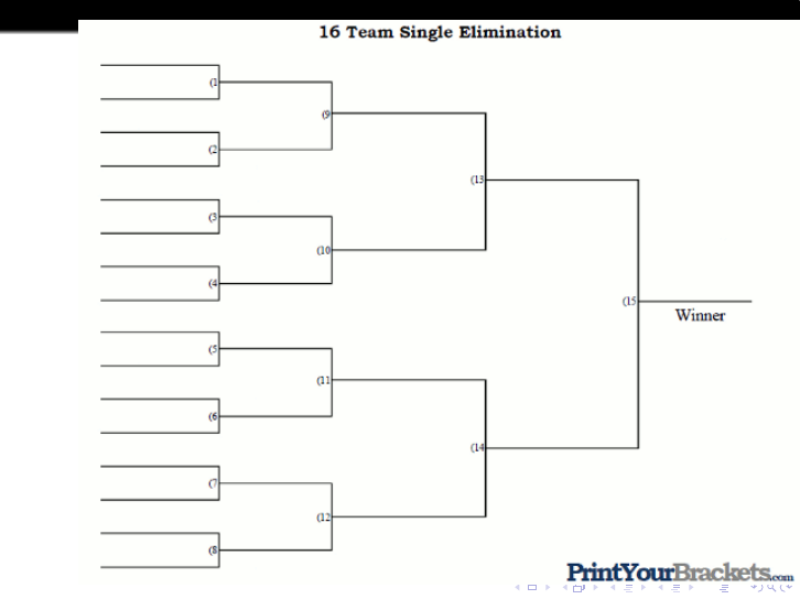
Robustness of second seed winning probability. A mathematically
natural model for relative strengths of top players is (βξ
i
, i ≥ 1) where
0 < β < ∞ is a scale parameter and
ξ
1
> ξ
2
> ξ
3
> . . .
form the inhomogeneous Poisson point process on R of intensity e
−x
arising in extreme value theory. So we can simulate a tournament, in the
conventional deterministic-over-seeds pattern to see which seed wins.
The next graphic gives data from simulations of such a tournament with
16 players, assuming the seeding order coincides with the strength order.
The interpretation of the parameter β is not so intuitive, but that
parameter determines the probability that the top seed would beat the
2nd seed in a single match, and this probability is shown (as a function of
β) in the top curve in Figure 1. The other curves show the probabilities
that the 16-player tournament is won by the players seeded as 1, 2, 3, 5
or 9.
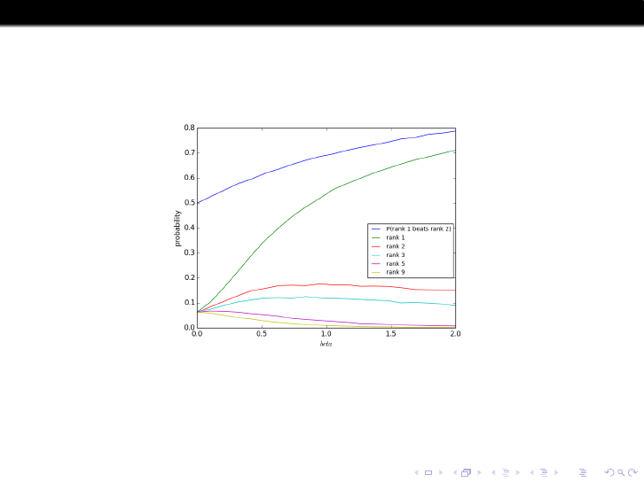
Figure: Probabilities of different-ranked players winning the tournament,
compared with probability that rank-1 player beats rank-2 player (top curve).
The results here are broadly in accord with intuition. For instance it is
obvious that the probability that the top seed is the winner is monotone
in β. What is perhaps surprising and noteworthy is that the probability
that the 2nd seed player is the winner is quite insensitive to parameter
values, away from the extremes, at around 17%.

Is this 17% prediction in fact accurate?
How robust is it to alternate models?
As a start, data from tennis tournaments
1
in Table 1 shows a moderately
good fit.
Table: Seed of winner, men’s and women’s singles, Grand Slam tennis
tournaments, 1968 - 2016.
seed of winner 1 2 3 4 5+ total
frequency 148 94 42 29 77 390
percentage 38% 24% 11% 7% 20% 100%
model, β = 0.65 41% 17 % 11 % 7 % 24% 100%
1
Wimbledon, and the U.S., French and Australian Opens form the prestigious
“Grand Slam” tournaments.

Reminder 4. Another aspect of what makes sports interesting to a
spectator is that strengths of teams change over time – if your team did
poorly last year, then you can hope it does better this year.
In the context of the Bradley-Terry model, one can extend the model to
allow changes in strengths. Seem to be about 2-3 academic papers per
year which introduce some such extended model and analyze some
specific sports data. Possible source of course projects – apply to
different sport or to more recent data.

Anchor data: [show World Football Elo ratings]
(1) The International football teams of Germany and France currently
(August 2017) have Elo ratimgs of 2080 and 1954, which (as described
later) can be interpreted as an implictly estimated probability 67% of
Germany winning a hypothetical upcoming match.
(2) Assertion Ratings tend to converge on a team’s true strength
relative to its competitors after about 30 matches.
Central questions.
(1) Why is there any connection between the ratings and probabilities?
(2) Is there any theory or data behind this thirty matches suffice
assertion?
Re (2), by analogy a search on seven shuffles suffice gets you to
discussions which can be tracked back to an actual theorem
Bayer-Diaconis (1992).
(Note project: math theory and data for card-shuffling).
History: Elo ratings originally used for chess, then for other individual
games like tennis, now widely used in online games. I write “player”
rather than team.


Idea 2: Elo-type rating systems
(not ELO). The particular type of rating systems we study are known
loosely as Elo-type systems and were first used systematically in chess.
The Wikipedia page Elo rating system is quite informative about the
history and practical implementation. What I describe here is an
abstracted “mathematically basic” form of such systems.
Each player i is given some initial rating, a real number y
i
. When player i
plays player j, the ratings of both players are updated using a function Υ
(Upsilon)
if i beats j then y
i
→ y
i
+ Υ(y
i
− y
j
) and y
j
→ y
j
− Υ(y
i
− y
j
)
if i loses to j then y
i
→ y
i
− Υ(y
j
− y
i
) and y
j
→ y
j
+ Υ(y
j
− y
i
) .
(2)
Note that the sum of all ratings remains constant; it is mathematically
natural to center so that this sum equals zero.

[Note: in practice the scheme is adapted to each specific sport, for
instance for International Football . . . ]
The*Elo*raSngs*are*based*on*the*following*formulas:
• R
n
*is*the*new*raSng,*R
o
*is*the*old*(preJmatch)*raSng.
• K*is*the*weight*constant*for*the*tournament*played:
• 60*for*World*Cup*finals;
• 50*for*conSnental*championship*finals*and*major*interconSn ental*to urnaments;
• 40*for*World*Cup*and*conSnental*qualifiers*and*major*tournaments;
• 30*for*all*other*tournaments;
• 20*for*friendly*matches.
• K*is*then*adjusted*for*the*goal*difference*in*the*game.*It*is*increased*by*half*if*a*
game*is*won*by*two*goals,*by*3/4*if*a*game*is*won*by*three*goals,*and*by*3/4$+$
(N=3)/8if*the*game*is*won*by*four*or*more*goals,*where*N*is*the*goal*difference.
• W*is*the*result*of*the*game*(1*for*a*win,*0.5*for*a*draw,*and*0*for*a*loss).
• W
e
*is*the*expected*result*(win*expectancy),*either*from*the*chart*or*the*following*
formula:
• W
e
*=*1*/*(10
(Jdr/400)
*+*1)
• dr*equals*the*difference*in*raSngs*plus*100*points*for*a*team*playing*at*home.


Math comments on the Elo-type rating algorithm.
We require the function Υ(u), −∞ < u < ∞ to satisfy the qualitative
conditions
Υ : R → (0, ∞) is continuous, strictly decreasing, and lim
u→∞
Υ(u) = 0.
(3)
We will also impose a quantitative condition
κ
Υ
:= sup
u
|Υ
0
(u)| < 1. (4)
To motivate the latter condition, the rating updates when a player with
(variable) strength x plays a player of fixed strength y are
x → x + Υ(x − y ) and x → x − Υ(y − x)
and we want these functions to be increasing functions of the starting strength
x.
Note that if Υ satisfies (3) then so does cΥ for any scaling factor c > 0. So
given any Υ satisfying (3) with κ
Υ
< ∞ we can scale to make a function where
(4) is satisfied.
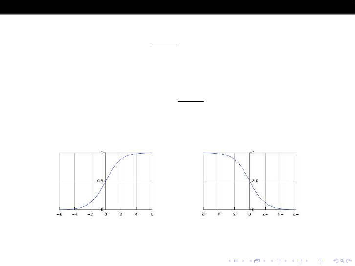
The logistic distribution function
F (x) :=
e
x
1 + e
x
, −∞ < x < ∞
is a common choice for the “win probability” function W (x) in the basic
probability model; and its complement
1 − F (x) = F (−x) =
1
1 + e
x
, −∞ < x < ∞
is a common choice for the “update function shape” Υ(x) in Elo-type
rating systems. That is, one commonly uses Υ(x) = cF(−x).
possible W (x) possible Υ(x)
Whether this is more than a convenient choice is a central issue in this
topic.

Elo is an algorithm for producing ratings (and therefore rankings) which
(unlike Bradley-Terry) does not assume any probability model. It
implicitly attempts to track changes in strength and puts greater weight
on more recent match results.
How good are Elo-type algorithms? This is a subtle question – we
need to
use Elo to make predictions
choose how to measure their accuracy
compare accuracy with predictions from some other ranking/rating
scheme (such as Bradley-Terry or gambling odds).
The simplest way to compare schemes would be to look at matches
where the different schemes ranked the teams in opposite ways, and see
which team actually won. But this is not statistically efficient [board].
Better to compare schemes which predict probabilities.
Although the Elo algorithm does not say anything explicitly about
probability, we can argue that it implicitly does predict winning
probabilities.

A math connection between the probability model and the rating
algorithm.
Consider n teams with unchanging strengths x
1
, . . . , x
n
, with match
results according to the basic probability model with win probability
function W , and ratings (y
i
) given by the update rule with update
function Υ. When team i plays team j, the expectation of the rating
change for i equals
Υ(y
i
− y
j
)W (x
i
− x
j
) − Υ(y
j
− y
i
)W (x
j
− x
i
). (5)
So consider the case where the functions Υ and W are related by
Υ(u)/Υ(−u) = W (−u)/W (u), −∞ < u < ∞.
In this case
(*) If it happens that the difference y
i
− y
j
in ratings of two
players playing a match equals the difference x
i
− x
j
in
strengths then the expectation of the change in rating
difference equals zero
whereas if unequal then (because Υ is decreasing) the expectation of
(y
i
− y
j
) − (x
i
− x
j
) is closer to zero after the match than before.

Υ(u)/Υ(−u) = W (−u)/W (u), −∞ < u < ∞. (6)
These observations suggest that, under relation (6), there will be a
tendency for player i’s rating y
i
to move towards its strength x
i
though
there will always be random fluctuations from individual matches. So if
we believe the basic probability model for some given W , then in a rating
system we should use an Υ that satisfies (6).
Now “everybody (in this field) knows” this connection, but nowhere is it
explained clearly and no-one seems to have thought it through
(practitioners focus on fine-tuning to a particular sport). The first
foundational question we might ask is
What is the solution of (6) for unknown Υ?
This can be viewed as the setup for a
mathematician/physicist/statistician/data scientist joke.

Problem. For given W solve
Υ(u)/Υ(−u) = W (−u)/W (u), −∞ < u < ∞.
Solution
physicist (Elo): Υ(u) = cW (−u)
mathematician: Υ(u) = W (−u)φ(u) for many symmetric φ(·).
statistician: Υ(u) = c
p
W (−u)/W (u) (variance-stabilizing φ).
data scientist: well I have this deep learning algorithm . . . . . .
These answers are all “wrong” for different reasons. I don’t have a good
answer to “what Υ to use?” for given W (project?). But the opposite
question is easy: given Υ, there is a unique “implied win-probability
function W ” given by
W
Υ
=
Υ(−u)
Υ(−u) + Υ(u)

Conclusion: Using Elo with a particular Υ is conceptually equivalent to
believing the basic probability model with
W
Υ
=
Υ(−u)
Υ(−u) + Υ(u)
Relating our math set-up to data
In published real-world data, ratings are integers, mostly in range
1000 − 2000. Basically, 1 standard unit (for logistic) in our model
corresponds to 174 rating points by convention. So the implied
probabilities are of the form [football]
P( Germany beats France ) = L((2080 − 1954)/174) = 0.67.
By convention a new player is given a 1500 rating. If players never
departed, the average rating would stay at 1500. However, players
leaving (and no re-centering) tends to make the average to drift upwards.
This makes it hard to compare “expert” in different sports.

My own, more mathematical write-up of this topic is in a paper Elo
Ratings and the Sports Model: a Neglected Topic in Applied
Probability?, and more possible projects are suggested there.
We have answered our first “central question”:
Central questions.
(1) Why is there any correction between the ratings and probabilities?
(2) Is there any theory or data behind this thirty matches suffice
assertion?
Recall that if strengths did not change then we can just use the basic
probability model and use MLEs of the strengths. The conceptual point
of Elo is to try to track changing strengths. So question (2) becomes
How well does Elo track changing strengths?

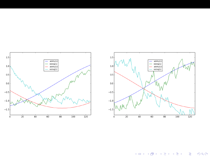
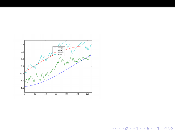
How well does Elo track changing strengths?
Too hard as theory – can only study via simulation. What do we need to
specify, to make a model we can simulate and assess?
1
Distribution of strengths of teams (at fixed time): has a “spread”
parameter σ
2
How strengths change with time (time-stationary): has a “relaxation
time” parameter τ
3
Scheduling of matches
4
Update function Υ and win-probability function W ; and a scale
constant c; update by cΥ(·)
5
Assess accuracy?
Item 2 is conceptually hardest . . . ; I use several “qualitatively extreme”
models. For item 3 I use random matching of all teams, each time unit.

For distribution of strengths use normal, σ = 0.5 or 1.0, which matches
real data. For changes in strengths over time use
Cyclic
Ornstein-Uhlenbeck (ARMA)
Hold (quite long time), jump to independent random.
each with a “relaxation time” parameter τ . For the win-probability
function W and the update function Υ use
Logistic
Cauchy
Linear over [−1, 1]
Use different scalings c for updates cΥ.

We need to quantify “ How well does Elo track changing strengths” in
some way. Here’s my way.
Consider players A, B at a given time with actual strengths x
A
, x
B
and
Elo ratings y
A
, y
B
. The actual probability (in our model) that A beats B
is W (x
A
− x
B
) whereas the probability estimated from Elo is
W (y
A
− y
B
). So we calculate
root-mean-square of the differences W (y
A
− y
B
) − W (x
A
− x
B
)
averaging over all players and all times. I call this RMSE-p, the “p” as a
reminder we’re estimating probabilities, not strengths.
Key question: If willing to believe that (with appropriate choices) this is
a reasonable model for real-world sports, what actual numerical values do
we expect for RMSE-p?
Short answer; No plausible model gives RMSE-p much below 10%.
This is when we are running models forever (i.e. stationary) so hard to
reconcile with “30 matches suffice”.


We can estimate the mismatch error from the deterministic limit in which
c → 0 for unchanging strengths.
Table: RMSE-p mismatch error.
W logistic logistic Cauchy Cauchy linear linear
Υ linear Cauchy logistic linear logistic Cauchy
σ = 0.5 0.9% 1.1% 1.2% 2.4% 3.2% 6.4%
σ =1.0 2.9% 2.9% 2.5% 5.4% 3.2% 6.0%
These errors are perhaps surprisingly small. Now let us take W and Υ as
logistic, so no mismatch error. The next table shows the effect of
changing the relaxation time τ of the strength change process.

Table: RMSE-p and (optimal c) for O-U model (top) and jump model (bottom)
τ
σ 50 100 200 400
0.5 12.9% 11.1% 9.5% 8.2 %
(0.11) (0.09) (0.08) (0.07)
1.0 17.0% 14.6 % 12.4% 10.4%
(0.28) (0.24) (0.16) (0.14 )
τ
σ 50 100 200 400
0.5 12.8% 11.2% 9.8% 8.4 %
(0.12) (0.09) (0.06) (0.05)
1.0 16.9% 14.5 % 12.4% 10.5%
0.30 0.24 0.19 0.14
This shows the intuitively obvious effect that for larger τ we can use smaller c
and get better estimates. But curious that numerics in the two models are very
close. One can do heuristics (and proofs if one really wanted to) for
order-of-magnitude scalings as c ↓ 0 but hardly relevant to real-world cases.

Bottom line from simulations: If you want RMSE-p to be noticeably
less than 10% then you need to have played 400 matches and you need
that strengths do not change substantially over 200 matches.
Games per year, regular season.
U.S. Football 16
Aussie Rules 22
U.K. Premier League 38
U.S. Basketball 82
U.S. Baseball 162

Some other aspects of rating models.
1. Recent book “The Science of Ranking and Rating” treats methods
using undergraduate linear algebra. The lecture in this course in 2014
was based more on that book (link on web page).
2. People who attempt realistic models of particular sports, using e.g.
statistics of individual player performance, believe their models are much
better than general-sport methods based only on history of wins/losses or
point differences. But a recent paper Statistics-free sports prediction
claims that (using more complex prediction schemes) they can do almost
as well using only match scores.
3. I have talked about comparing different schemes which predict
probabilities – after we see the actual match results, how do we decide
which scheme is better? I will discuss this in a different context, the
lecture on Geopolitics forecasting.
4. Both schemes are poor at assessing new players. Xbox Live uses its
“TrueSkill ranking system” [show page] which estimates both a rating
and the uncertainty in the rating, as follows.


Here a rating for player i is a pair (µ
i
, σ
i
), and the essence of the scheme
is as follows. When i beats j
(i) first compute the conditional distribution of X
i
given X
i
> X
j
, where
X
i
has Normal(µ
i
, σ
2
i
) distribution
(ii) then update i’s rating to the mean and s.d. of that conditional
distribution.
Similarly if i loses to j then i’s rating is updated to the mean and s.d. of
the conditional distribution of X
i
given X
i
< X
j
.
Discussion. The authors seem to view this as an
approximation to some coherent Bayes scheme, but to me it
fails to engage both ‘‘uncertainty about strength" and
‘‘uncertainty about match outcome".
So another simulation project is to compare this to other schemes. Note
this implicitly predicts winning probabilities via P(X
i
> X
j
).

