Measuring Private Equity Fund Performance

Measuring Private Equity

Fund Performance

BACKGROUND NOTE

02/2019-6472

This background note was written by Alexandra Albers-Schoenberg, Associate Director at INSEAD’s Global Private

Equity Initiative (GPEI), under the supervision of Claudia Zeisberger, Professor of Entrepreneurship at INSEAD and

Academic Director of the GPEI. We wish to thank Michael Prahl and Bowen White, both INSEAD alumni, for their

significant input prior to completion of this note. It is intended to be used as a basis for class discussion rather than to

illustrate either effective or ineffective handling of an administrative situation.

Additional material about INSEAD case studies (e.g., videos, spreadsheets, links) can be accessed at cases.insead.edu.

THIS NOTE IS MADE AVAILABLE BY INSEAD FOR PERSONAL USE ONLY. NO PART OF THIS PUBLICATION MAY BE TRANSLATED, COPIED, STORED, TRANSMITTED,

REPRODUCED OR DISTRIBUTED IN ANY FORM OR MEDIUM WHATSOEVER WITHOUT THE PERMISSION OF THE COPYRIGHT OWNER.

Performance in private equity investing is traditionally measured via (i) the internal rate of return

(IRR) which captures a fund’s time-adjusted return, and (ii) multiple of money (MoM) which

captures return on invested capital. Once all investments have been exited and the capital returned

to limited partners, the final return determines the fund’s standing amongst its peers, i.e., those

from the same vintage with a similar investment strategy and geographic mandate. Whether it is in

the top quartile is the question.

However, IRR and MoM, merely provide a first layer of insight into private equity fund

performance. Other metrics offer a more nuanced view of performance over the life of the fund,

and by various adjustments offer a return picture that is more comparable to the performance of

public equity markets and other liquid asset classes. This paper explains the various metrics

employed by general partners (GPs) and limited partners (LPs) to arrive at a meaningful assessment

of a fund’s success.

Internal Rate of Return (IRR)

IRR, the performance metric of choice in the PE industry, represents the discount rate that renders

the net present value (NPV) of a series of investments zero. IRR reflects the performance of a

private equity fund by taking into account the size and timing of its cash flows (capital calls and

distributions) and its net asset value at the time of the calculation.

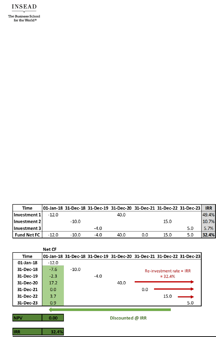
Exhibit 1 shows the various calls, distributions and net cash flow for a hypothetical fund. Negative

cash flows = capital calls; positive cash flows = distributions.

Exhibit 1

Despite its widespread acceptance, the assumptions underlying the IRR calculation and its practical

application have created controversy. One of its main weaknesses is the built-in “reinvestment

assumption” that capital distributed to LPs early on will be reinvested over the life of the fund at

the same IRR as generated at the initial exit. Hence a high IRR (>25%) generated by a successful

exit early in a PE fund’s life is likely to overstate actual economic performance, as the probability

of finding an investment with a comparably high IRR over the remaining (short) term is low. This

is particularly true as the nature of PE funds (all capital committed upfront) prohibits investors

from reinvesting capital in other funds in the divestment stage (which would be the closest in terms

of risk-return proposition to the exited investment). The mechanics of the IRR calculation thus

provide an incentive for GPs to aggressively exit portfolio companies early in a fund’s lifecycle to

“lock in” a high IRR. A related problem, although smaller in magnitude, is that IRR fails to take

into account the LP’s cost of holding capital until it is called for investment.

Beyond these weaknesses, there are two additional problems. First is variability in how the metric

is applied by GPs to aggregate the IRRs of individual portfolio investments to arrive at a fund-

level return. In the absence of a clear industry standard, comparisons between fund IRRs are

difficult. Second, the IRR is an absolute measure and does not calculate performance relative to a

benchmark or market return, making comparisons between private and public equity (and other

asset classes) impossible.

Modified IRR (MIRR)

MIRR overcomes the reinvestment assumption problem of the standard IRR model by assuming

that positive cash flows to LPs are reinvested at a more realistic expected return (such as the

average PE asset class returns or public market benchmark); it also accounts for the cost of uncalled

capital, unlike the standard IRR model. By basing the IRR on more realistic assumptions for both

reinvestment and cost of capital, MIRR provides a more accurate measure of PE performance.

The effects of switching from IRR to MIRR for a given portfolio are as follows: astronomic 100%+

IRRs for “star” funds resulting from early exits are brought down into more reasonable territory,

while funds suffering from early poor performing exits are no longer penalized on the unreasonable

assumption that all investments (and even uninvested capital) will lose money. The MIRR method

generally results in less extreme performance by both strong and weak funds.

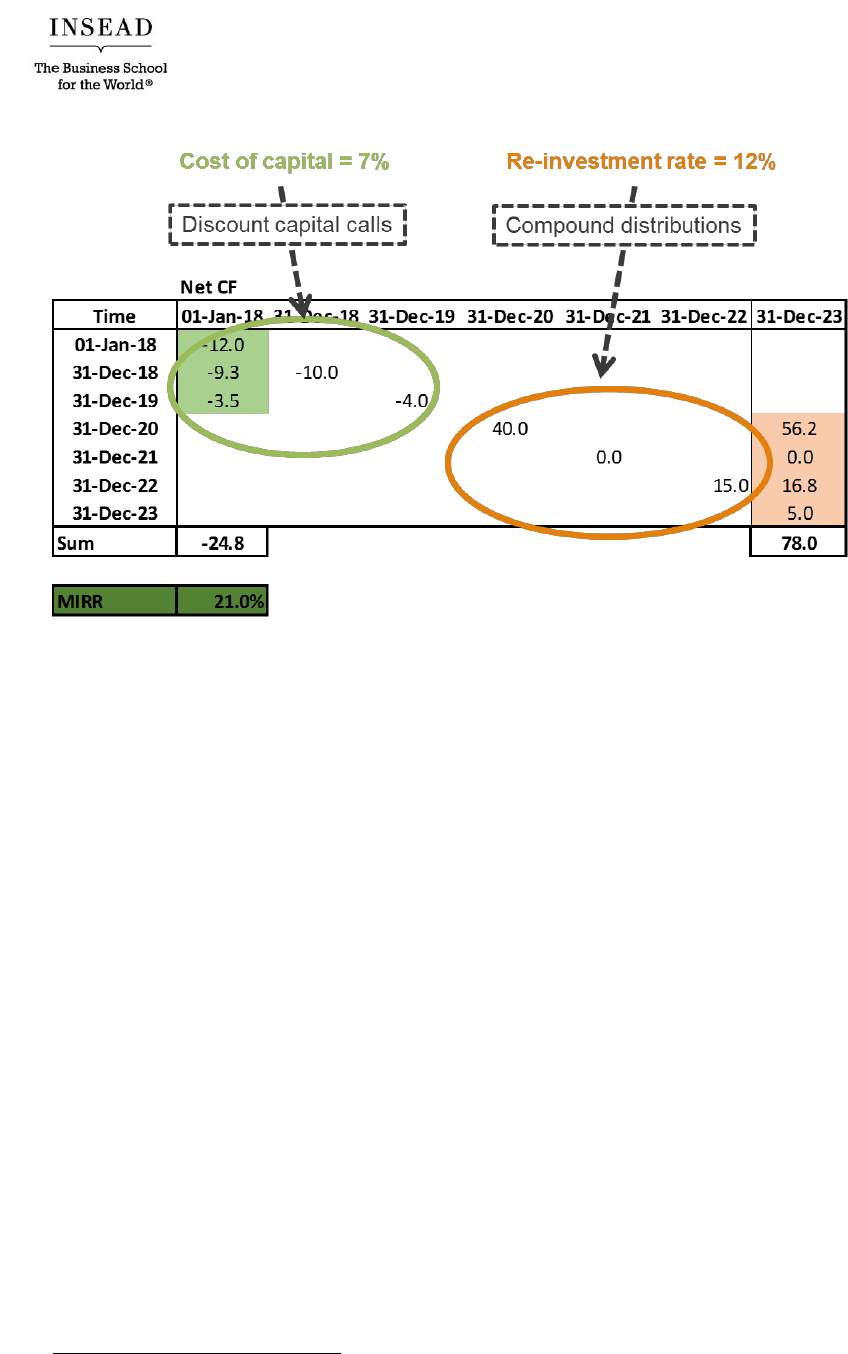
A simple example of how the MIRR works is provided below.

Exhibit 2

In the MIRR methodology, original fund cash flows are modified by discounting all capital calls

to year 0 at a defined discount rate and compounding all distributions to the valuation date at a

defined reinvestment rate. The discount rate is set at 7% and the reinvestment rate at 12% in our

example.

Calculating the IRR of the modified fund cash flows (i.e. -24.8 at year 0 and 78.0 at year

6) produces the fund’s MIRR (21.0%) for a discount rate of 7% and a reinvestment rate of 12%.

In this example, the MIRR (21.0%) significantly differs from the IRR (32.4%), because of the high

early exit (+40) in year 3 of transaction 1.

Money Multiples

A private equity fund’s multiple of money invested (MoM) is represented by its total value to paid-

in ratio (TVPI).

The TVPI consists of a fund’s residual value to paid-in ratio (RVPI) and its

distributed to paid-in ratio (DPI). That is, TVPI = RVPI + DPI.

To understand how these ratios evolve over a fund’s life, the following definitions are helpful.

 The “paid-in” (PI) in TVPI, DPI and RVPI represents the total amount of capital called by

a fund (for investment and to pay management and other fees)

at any given time.

 The “distributed” (D) in DPI represents capital that has been returned to fund investors

following the sale of a fund’s stake in a portfolio company.

 The “residual value” (RV) in RVPI represents the fair value of the stakes that a fund holds

in its portfolio companies and is measured by its net asset value (NAV).

The 7% cost of capital &the 12% re-investment rate in this example was freely chosen. The re-investment rate is

an approximation of a long-term average of PE gross returns.

The MIRR of a set of cash flows can also be calculated in Excel with the MIRR function, in which the discount

and re-investment rates are set.

MoM is also often referred to as Multiple on Invested Capital (MOIC).

Other fees include transaction, portfolio company, monitoring, broken deal, and directors’ fees.

Therefore:

 Residual value to paid-in (RVPI) represents the fair value of a fund’s investment portfolio

(or NAV) divided by its capital calls at the valuation date, hence RVPI is the portion of a

fund’s value that is unrealized. It is higher at the beginning,

when the majority of fund

value resides in active portfolio companies. As the fund ages and investments are exited,

RVPI will decrease to zero.

RVPI = NAV / LP Capital called

 Distribution to paid-in (DPI) represents the amount of capital returned to investors

divided by a fund’s capital calls at the valuation date. DPI reflects the realized, cash-on-

cash returns generated by its investments at the valuation date. It is most prominent once

the fund starts exiting investments, particularly towards the end of its life. If the fund has

not made any full or partial exits, the DPI will be zero.

DPI = sum of proceeds to fund LPs / LP capital called

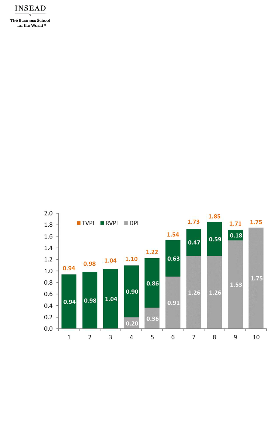
Exhibit 3 shows the evolution of the TVPI, DPI and RVPI for a hypothetical fund over its entire

life.

Exhibit 3

The evolution of TVPI, DPI and RVPI reflect the pattern of investment and divestment in a typical

private equity fund structured as a limited partnership.

0. Before the fund draws capital and invests, there is already a drag from fees paid upfront in

connection with setting up and managing the fund and its operations, which results in a

TVPI < 1 in the first period.

RVPI can also be higher midway if an investment is written up.

1. Early in the fund’s life, as it deploys fund capital into portfolio companies, the majority of

value is unrealized and captured by its RVPI. In our example, the fund deploys capital from

years 1 to 3 without divesting any assets.

2. As the fund’s investments begin to mature and are exited, portions of its value are realized

and reflected in its DPI. In our example, the fund’s first exit took place in year 4, producing

a DPI of 0.20.

3. The share of the fund’s DPI continues to rise (and RVPI to fall) until all of its investments

have been exited, at which point all value has been realized and is captured by a fund’s

DPI. The final DPI reflects its cash-on-cash MoM. In our example, the fund generated a

cash-on-cash return of 1.75x for investors. It is important to note that the NAV fluctuates

over time (e.g. 185 at some point, but lower eventual realisations.)

Comparing PE with Public Equity Portfolios

LP investment committees often ask to compare PE funds’ performance with that of more

traditional asset classes, which is far from straightforward. Unlike listed or traded instruments,

much of PE’s performance reporting relies on interim valuations of unlisted and illiquid

investments (i.e. the components of a fund’s NAV), making precise “mark-to-market” impossible.

Furthermore, PE is dominated by outliers, which are difficult to “index”, and its risk-return patterns

are quite distinct from more traditional asset classes. It is challenging to gain broad (index-like)

exposure to PE, unlike public markets where building a diversified portfolio is quite

straightforward.

Moreover, the standard performance measures in PE – IRR and MoM – are not directly comparable

to liquid asset classes where valuations and returns are easily determined through a daily mark-to-

market. IRR takes into account the timing and size of cash flows, while public equity benchmarks

use time-weighted return measures. Despite the problem of comparing apples to oranges, attempts

have been made to arrive at a (somewhat) realistic comparison, as detailed below.

Public Market Equivalent (PME)

A frequently cited method is the public market equivalent (PME) approach, an index-return

measure that takes the irregular timing of cash flows in PE into account. PME compares an

investment in a PE fund to an equivalent investment in a public market benchmark (e.g. the S&P

500). Selecting the right index when using a PME method to find alpha is important, as different

indices can provide a completely different picture.

Below we describe the most commonly used PME methodologies.

Long-Nickels PME (LN PME): The first PME method was developed by Long and Nickels in

1996.

It compares the performance of a PE fund with a benchmark by creating a theoretical

investment in the index using the fund’s cash flows. It assumes that all cash flows resulting from

capital calls or distributions from the PE fund are replicated in a public market index; the returns

generated by these evolve over time, mirroring the index. The LN PME then compares the IRR

RVPI can be higher than 1 with no realisations and a fee drag, if there is a write up on the basis of the fair market

value.

Long, A.M. III & Nickels, C.J. (1996). A Private Investment Benchmark. The University of Texas System, AIMR

Conference on Venture Capital Investing.

generated by the investment in the index and the IRR generated by the fund to gauge

out/underperformance. Put simply, every capital call from the PE fund triggers an equivalent

purchase in the public market index and every distribution triggers a sale of the respective index

stake.

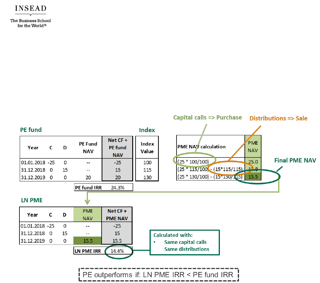
An example of how the LN PME works is provided below:

Exhibit 4

The cash flows – i.e. capital calls (C) and distributions (D) – generated by the PE fund are adjusted

based on the performance of the index to generate the NAV of the PME replicating portfolio (PME

NAV in our chart). A negative net cash flow, i.e. a capital call, leads to a purchase of equal value

of the indexed asset. For example, the -$25 of net cash flow in period 0 (01.01.2018) is matched

by a $25 purchase of an indexed asset. A positive net cash flow, i.e. a distribution, leads to a sale

of equal value of the indexed asset. For example, the $15 of net cash flow in period 1 (31.12.2018)

is matched by a $15 sale of the indexed asset.

It is important to note that the value of each purchase or sale of the indexed asset evolves as the

index evolves, i.e. value increases or decreases with the movements of the index over time. For

example, the value attributed to the original -25 capital call is 25 (25 * 100/100) at the end of period

0; 28.75 (25 * 115/100) at the end of period 1; 32.5 (25 * 130/100) at the end of period 2, and so

on. In the end, the IRR of the fund is compared to the PME IRR of the theoretical investment; the

PME-NAV simply replaces the fund NAV for the PME IRR calculation. PE outperforms if the PE

fund IRR is larger than the estimated PME IRR.

The LN PME allows for a direct comparison between PE fund returns and public market returns.

However, in a case of high PE fund distributions (e.g. by a high-performing fund), the mechanics

of the LN PME may produce a negative PME NAV, effectively resulting in a short position in the

index.

The PME+ and the PME were developed to address this shortcoming, both of which use a co-

efficient to re-scale the private equity fund’s distributions so the public market NAV does not go

negative.

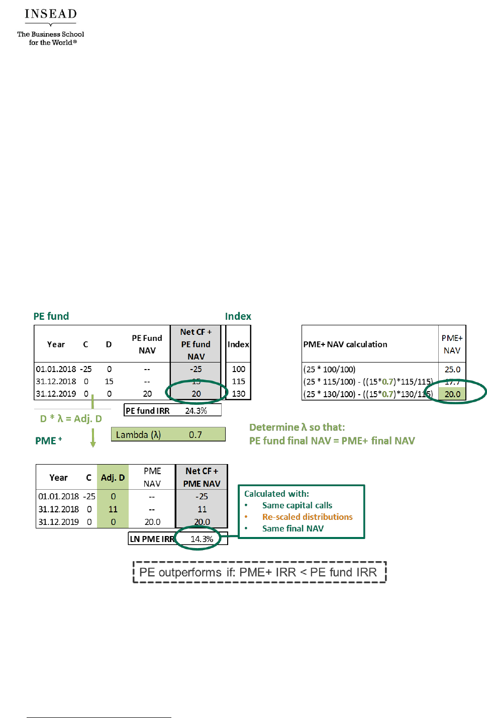
PME+:

The PME+ follows the same principle as the PME. Again, a theoretical investment is

made in the index by using the fund’s cash flows. This time, however, the distributions are re-

scaled by a factor lambda so that the PME NAVs can’t be negative. The lambda is chosen so that

the final PME NAV is the same as the final PE fund NAV. The re-scaled distributions are then

used to calculate an IRR for the theoretical investment. PE outperforms if the calculated PME+

IRR is smaller than the IRR of the PE fund.

An example of how the PME+ works is provided below:

Exhibit 5

Like the LN PME, the PME+ allows for a direct comparison between the PME+ IRR and the PE

fund IRR, and avoids negative PME NAVs. One weakness, however, is that it does not match the

cash flows perfectly.

Kaplan Schoar PME (KS PME):

The Kaplan Schoar PME measures the wealth multiple effect

of investing in the PE fund versus the index. It represents the market-adjusted equivalent to the

traditional TVPI. The KS PME incorporates the performance contribution of a public market index

by compounding each fund cash flow – both capital calls and distributions – based on index

Rouvinez, C. (2003) “Private equity benchmarking with PME+. Private Equity International, August, 34–38.

Kaplan, S. & Schoar, A. (2005). Private Equity Performance: Returns, Persistence, and Capital Flows. Journal

of Finance, 60, 1791–1823.

performance; index performance is measured between the date of the cash flow and the valuation

date. When the fund’s actual NAV is added to the compounded distributions and divided by the

compounded capital calls, KS PME produces a multiple that represents the out/underperformance

of the PE fund relative to the market index.

If the KS PME is greater than 1, the PE fund

outperformed the public market index.

KS PME = (Sum of future value distributions + NAV) / Sum of future value capital calls

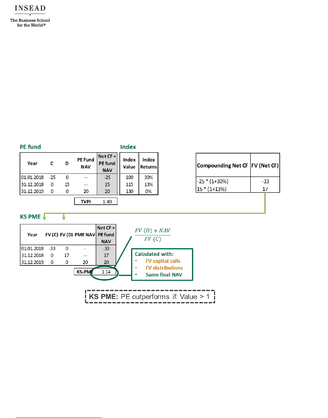
A numerical example is provided below using the same fund cash flows and index performance

used in the LN PME.

Exhibit 6

In the example, we include the returns generated by the index in a separate column. Compounding

the cash flows by these returns generates the corresponding future cash flow of the capital call or

the distribution [i.e. FV (C) or FV (D)]. The 1.14 KS PME statistic generated represents the

outperformance of the PE fund.

The KS PME is easy to calculate and does not have the flaws of an IRR calculation, However, it

ignores the timing of cash flows.

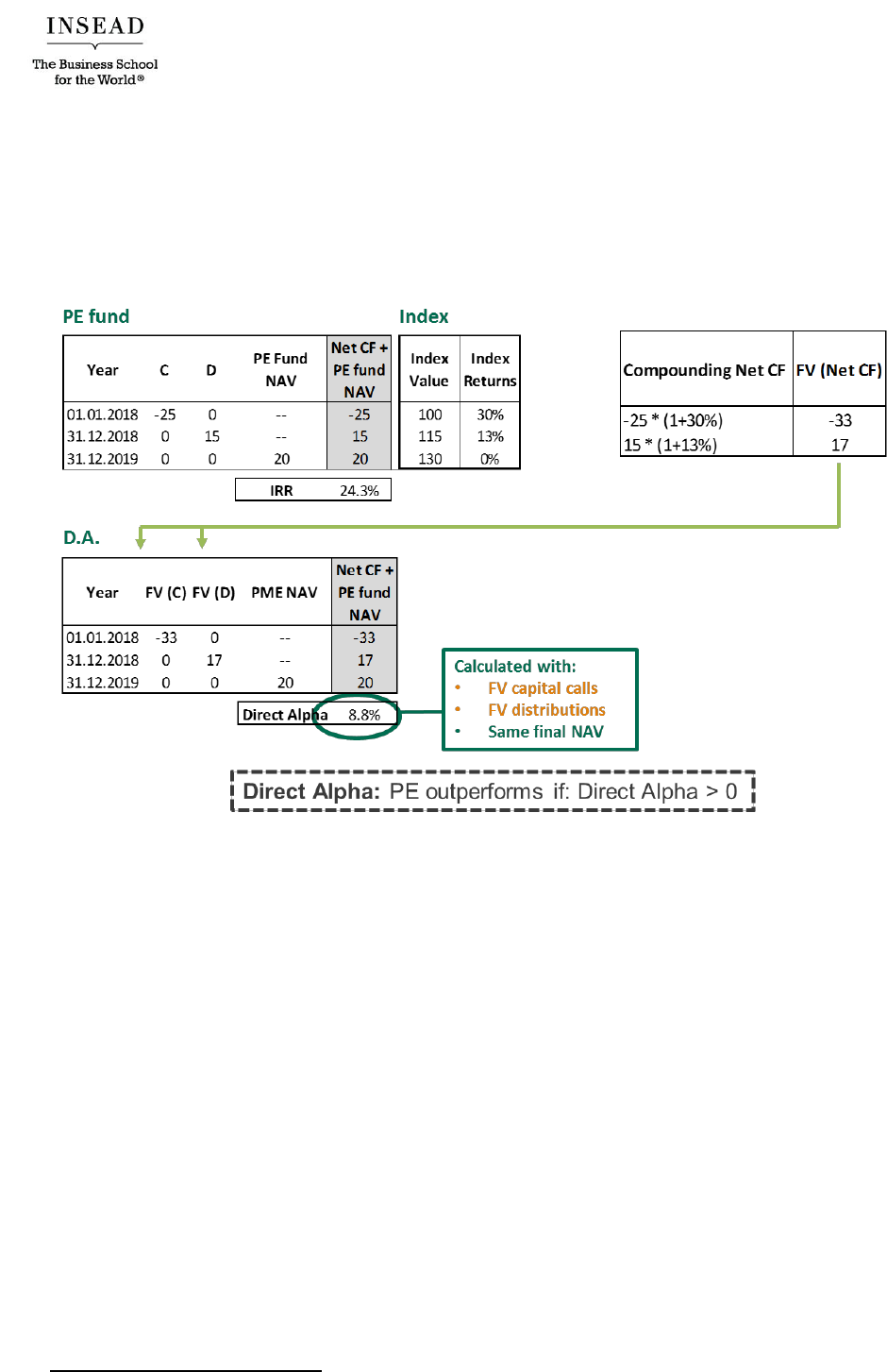
Direct Alpha

The most recent method to compare private equity returns against public markets is the so-called

direct alpha.

This has much in common with the KS PME, and uses the exact same methodology

Note that cash flows can be discounted rather than compounded, along with the fund’s NAV, and the same KS

PME MoM will be produced.

Griffiths, B. (2009). Estimating Alpha in Private Equity, in Oliver Gottschalg (ed.), Private Equity Mathematics,

2009, PEI Media.

to adjust the cash flows (i.e. compounding by index performance).

The key difference is that

direct alpha quantifies the out/underperformance of the PE fund by calculating the IRR of the

compounded cash flows plus fund NAV, rather than a multiple of performance. An example is

provided below.

Exhibit 7

In the example, the fund has an IRR of 24.3% and a direct alpha of 8.8%, attributing an IRR of

15.5% to the market over the period.

Direct alpha tries to overcome some flaws of the PME methods and is the only method to calculate

the exact rate of return of outperformance, rather than an approximation.

Similar to the KS PME, the cash flows and the fund NAV can also be discounted, and will produce the same KS

PME statistic.

Summary

The table below provides an overview of the relationship between the absolute and the market-

adjusted performance measures. LN PME, PME+ and direct alpha are the market-adjusted

equivalents of the traditional IRR and the MIRR of a PE fund. The KS PME is the market-adjusted

equivalent of the traditional TVPI.

Rate of return

Total return

Absolute return

IRR,

MIRR

MoM (TVPI)

Market-adjusted

return

LN PME,

PME+,

Direct Alpha

KS PME

The private equity asset class has unique characteristics, including the irregular timing and

size of cash flows, making measurement of returns far from straightforward and difficult to

benchmark with other asset classes. The widely used IRR and MoM return measures have

their own flaws and are not ideal to portray and compare PE return figures. As the market

is maturing, there is hope that more sophisticated measures may become standard. It is up

to LPs, as multi-asset class investors, to promote and request them.

Additional reading

Zeisberger, C., Prahl, M. & White, B. (2017). Mastering Private Equity: Transformation via

Venture Capital, Minority Investments and Buyouts. Wiley: Hoboken, New Jersey.

Preqin. (2015, July). Preqin Special Report: Public Market Equivalent (PME) Benchmarking.

Retrieved from http://docs.preqin.com/reports/Preqin-Special-Report-PME-July-2015.pdf

eVestment. (2017, September). Enhancing Private Equity Manager Selection with Deeper Data.

Retrieved from https://www.evestment.com/wp-content/uploads/2017/09/eVestment-Enhancing-

Private-Equity-Manager-Selection-with-Deeper-Data.pdf

Capital Dynamics. (2015, July). Public benchmarking of private equity Quantifying the shortness

issue of PME. Retrieved from https://www.capdyn.com/media/1813/white-paper-shortness-final-

30jul2015.pdf

Griffiths, B. (2009). Estimating Alpha in Private Equity, in Oliver Gottschalg (ed.), Private Equity

Mathematics, 2009, PEI Media.

Kaplan, S. & Schoar, A. (2005). Private Equity Performance: Returns, Persistence, and Capital

Flows. Journal of Finance, 60, 1791–1823.

Long, A.M. III & Nickels, C.J. (1996). A Private Investment Benchmark. The University of Texas

System, AIMR Conference on Venture Capital Investing.

Rouvinez, C. (2003) “Private equity benchmarking with PME+. Private Equity International,

August, 34–38.

Stucke, R., Griffiths, B.E. & Charles, I.H. (2014, March). An ABC of PME. Retrieved from

https://www.secondariesinvestor.com/wp-content/uploads/sites/3/2014/03/An-ABC-of-PME-

Landmark-Partners.pdf