Fiscal policy coordination in currency unions

at the eﬀective lower bound

Thomas Hettig and Gernot J. M¨uller

∗

January 2017

Abstract

According to the pre-crises consensus there are separate domains for monetary and ﬁscal

stabilization in a currency union. While the common monetary policy takes care of union-

wide ﬂuctuations, ﬁscal policies should be tailored to meet country-speciﬁc conditions.

This separation is no longer optimal, however, if monetary policy is constrained by an

eﬀective lower bound on interest rates. Speciﬁcally, we show that in this case there are

beneﬁts from coordinating ﬁscal policies across countries. By coordinating on a common

ﬁscal stance, policy makers are able to stabilize union-wide activity and inﬂation while

avoiding detrimental movements of a country’s terms of trade.

Keywords: Currency union, ﬁscal policy, eﬀective lower bound, coordination,

EMU, terms-of-trade externality, optimal policy

JEL-Codes: E61, E62, F41

∗

Hettig: Bonn Graduate School of Economics and University of T¨ubingen; Email: thomas.hettig@uni-

tuebingen.de; M¨uller: University of T¨ubingen, CESifo and CEPR, London; Email: gernot.mueller@uni-

tuebingen.de. We thank Yao Chen, Cyntia Freitas Azevedo, Fabio Ghironi, Martin Hellwig, Keith Kuester,

Klaus Prettner, Joost R¨ottger, Alexander Scheer, Martin Wolf, and participants in various seminars and con-

ferences for helpful comments and discussions. Part of this research was conducted while Hettig visited the

Brazilian Central Bank in Bras´ılia and he would like to thank the research department for its hospitality. We

also gratefully acknowledge ﬁnancial support by the German Science Foundation (DFG) under the Priority

Program 1578. The usual disclaimer applies.

1 Introduction

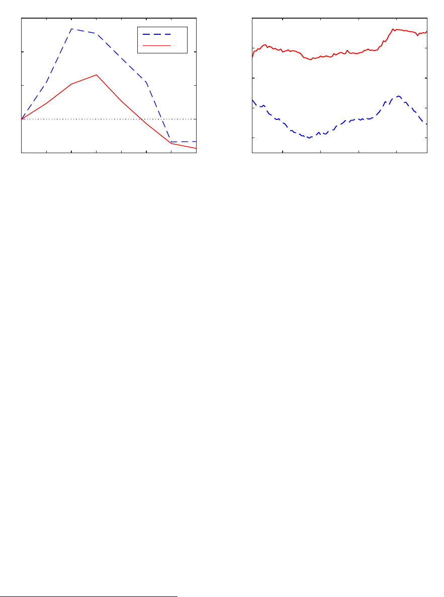
In the wake of the global ﬁnancial crisis, ﬁscal policy staged a comeback as a stabilization tool.

Figure 1 displays two rough measures of the discretionary ﬁscal stance, both for the US and

the euro area. The left panel shows the change of the cyclically adjusted government budget

deﬁcit, measured in percentage-point changes relative to the pre-crisis year 2007. The right

panel shows the level of government consumption relative to trend output. Both measures

are indicative of an expansionary ﬁscal stance during the recession: deﬁcits rose sharply after

2007, as did government spending. It appears, however, that ﬁscal stabilization has been used

more timidly in the euro area: not only did deﬁcits increase less than in the US, government

spending was also raised relatively less, given its higher pre-crisis level.

One possible explanation is that euro-area ﬁscal policy is largely determined at the country

level, rather than at the union level and, hence, there may have been a failure to coordinate

ﬁscal stabilization across the member states of the euro area.

In line with this conjecture,

there have been calls for stronger policy coordination, urging European governments to en-

gineer a larger ﬁscal expansion during 2008–09 (see, for instance, Krugman, 2008). For the

same reason, the shift to austerity in the euro area after 2010 may have been excessive, as

argued by many observers (see, for instance, Cotarelli, 2012). Against this background, we

ask whether ﬁscal-stabilization policies should be coordinated across the member states of a

currency union with a view towards stabilizing area-wide activity and inﬂation.

According to the pre-crises consensus ﬁscal stabilization should be geared towards country-

speciﬁc conditions, because the common monetary policy can take care of union-wide ﬂuctu-

ations (Beetsma and Jensen, 2005; Kirsanova et al., 2007; Gal´ı and Monacelli, 2008).

The

recent economic and ﬁnancial crises have exposed a shortcoming of this paradigm: in a se-

vere economic downturn monetary policy may be constrained by an eﬀective lower bound

(ELB) on nominal interest rates and thus be unable to stabilize ﬂuctuations at the union

level. Moreover, it is precisely under these circumstances that ﬁscal policy is very eﬀective in

stabilizing economic activity (Christiano et al., 2011; Woodford, 2011).

In our analysis we therefore explicitly account for the possibility that an ELB constrains

To be sure, there has been an attempt to coordinate European ﬁscal stabilization policies, namely through

the European Economic Recovery Plan, discussed and legislated in 2008–09. According to Cwik and Wieland

(2011) the measures foreseen by the plan amounted to 1.04 and 0.86 percent of 2009 and 2010 GDP, respectively.

Hence, they were considerably smaller than those due to US legislation under the American Recovery and

Reinvestment Act which amounted to roughly 5 percent of GDP.

Earlier contributions also allow for the possibility that the objectives of monetary and ﬁscal policy diﬀer.

This does not necessarily strengthen the case for coordination (Dixit and Lambertini, 2003). In fact, ﬁscal

coordination may even be harmful (Beetsma and Bovenberg, 1998). Dixit and Lambertini (2001) oﬀer some

qualiﬁcations as well as further references. Schmidt (2013) studies coordinated monetary and ﬁscal stabilization

in a closed economy when an eﬀective bound on interest rates binds.

2007 2008 2009 2010 2011 2012 2013 2014

-2

Budget deficit

1995 2000 2005 2010

0.14

0.16

0.18

0.2

0.22

Government consumption

Figure 1: Euro area (EA): solid lines, United Staates (US): dashed lines; left panel: cyclically

adjusted deﬁcit, annual observations, change relative to 2007, measured in percentage points

of potential output; right panel: government consumption of general government in units of

trend output, quarterly observations; source: OECD Economic Outlook.

monetary policy. We do so within the framework of Gal´ı and Monacelli (2008). It speciﬁes

a currency union which consists of a continuum of small open economies, each negligible in

terms of aggregate outcomes. Yet as countries specialize in the production of a speciﬁc set of

goods, domestic policies—if enacted unilaterally—will generally impact a country’s terms of

trade. In the absence of policy coordination, the optimal policy will therefore be conducted

with a view towards its eﬀect on the terms of trade. Instead, by coordinating on a common

policy, countries can internalize this “terms-of-trade externality”.

Hence, optimal policies

will generally diﬀer depending on whether there is coordination across countries or not.

In terms of country-speciﬁc policies, we focus on government spending. We assume that

the government purchases only domestically produced goods, ﬁnanced by lump-sum taxes

levied on domestic households. We consider a representative household in each country which

supplies labor and trades a complete set of state-contingent assets across countries. Its con-

sumption basket includes goods produced in all countries of the union, but is biased towards

domestically produced goods. Goods, in turn, are produced in a monopolistic competitive

environment and ﬁrms are restricted in their ability to adjust prices. In “normal” (or pre-

crisis) times monetary policy is able to perfectly stabilize inﬂation and output at the union

level: there is no need for ﬁscal coordination across countries. We contrast this situation

with a “crisis scenario” where monetary policy is unable to lower interest rates suﬃciently in

See Corsetti and Pesenti (2001), Benigno and Benigno (2003), De Paoli (2009) and Forlati (2015) for

diﬀerent perspectives on the terms-of-trade externality in the context of monetary policy.

response to a union-wide contractionary shock, because it is constrained by an ELB.

We determine the optimal discretionary adjustment of government spending in the crisis

scenario. Under coordination ﬁscal policies are set to maximize union-wide welfare. In the

absence of coordination ﬁscal policy makers maximize country-speciﬁc welfare. We ﬁnd that—

in line with the conjecture above—countries provide too little stimulus at the ELB in the

absence of coordination. Intuitively, local policymakers are keen to avoid the terms of trade

appreciating too much with higher spending, as this lowers the demand for domestically

produced goods at times of economic slack. Conversely, the increase of government spending

is higher under coordination, because policy makers anticipate that the terms of trade remain

unaﬀected by a policy response which is common across countries. At the same time, such a

response is expected to boost union-wide inﬂation (rather than an individual country’s terms

of trade). This is desirable at the ELB, because expected inﬂation lowers the real interest rate.

We illustrate that the ﬁscal stimulus gap due to the lack of coordination can be quantitatively

signiﬁcant.

Within our framework we recoup two results which have already been established in the

literature, but are crucial to put our main result into perspective. First, we conﬁrm an

earlier ﬁnding of Turnovsky (1988) and Devereux (1991): absent cooperation policy makers

choose too high a level of government spending in steady state. This is because governments

seek to improve their country’s terms of trade through purchases of domestically produced

goods.

Hence, in steady state the terms-of-trade externality has the opposite eﬀect than

in the crisis scenario, because stronger terms of trade are beneﬁcial in the long run, as the

economy operates at full capacity.

Second, we also contrast government spending multipliers, that is, the percentage change

of domestic output given a (possibly non-optimal) increase of government spending by one

percent of GDP in the entire union and in the domestic economy only. In line with earlier

work by Fahri and Werning (2016), we ﬁnd that the multiplier is larger than unity in the

ﬁrst case, provided the ELB binds, but smaller than unity in the second case.

This result

We abstract from non-conventional policies such as forward guidance (Eggertsson and Woodford, 2003)

or credit policies by the central bank (see, e.g., C´urdia and Woodford, 2011). These policies are arguably an

imperfect substitute for conventional policies, if only because they are not very well understood and hence

controversial (see, e.g., Rogoﬀ, 2016). The eﬀectiveness of forward guidance, in particular, appears to be

limited (Giannoni et al., 2016).

Epifani and Gancia (2009) ﬁnd that this mechanism may account for the size of the public sector in open

economies. In particular, their ﬁndings suggest that the terms-of-trade externality rather than a demand for

insurance causes the public sector to grow with trade openness.

Erceg and Lind´e (2012) also compute spending multipliers for a small open economy. Assuming an exchange

rate peg, they show that multipliers are always below unity. Assuming a speciﬁc scenario under which the

ELB binds, they ﬁnd that for multipliers to exceed unity prices need to be suﬃciently ﬂexible. Nakamura

and Steinsson (2014), in turn, show that multipliers are high within a currency union when compared to the

multiplier at the union level in the absence of a binding ELB constraint. Acconcia et al. (2014) ﬁnd for Italian

obtains because a unilateral increase of government spending appreciates the terms of trade

and thus crowds out private expenditure. Instead, the cooperative policy, common to all

countries, raises expected inﬂation at the union level, thus crowding-in private expenditure

at the ELB.

Our analysis also relates to a number of other recent studies. Cook and Devereux (2011)

study optimal ﬁscal policy in a two-country model when monetary policy is stuck at the

ELB. However, they focus on the case of coordination, rather than on a possible coordination

failure. Blanchard et al. (2016) calibrate a two-country model to capture key features of

the euro area, notably of its core and periphery. They share our focus on the gains from

cooperation. However, because their model is more complex than ours, their analysis is limited

to numerical evaluations of an ad-hoc welfare criterion. Evers (2015) studies the performance

of alternative ﬁscal arrangements in a quantitative model of a currency union. He ﬁnds that

a centralized ﬁscal authority dominates a regime of ﬁscal transfers as well as a regime of

decentralized ﬁscal decision making. Other work has focused on the coordination of debt and

deﬁcit policies in currency unions (Beetsma and Uhlig, 1999; Krogstrup and Wyplosz, 2010).

We abstract from this aspect, as Ricardian equivalence obtains in our model. Moreover, we

stress that our analysis disregards complications due to sovereign risk. However, both aspects

are likely to further strengthen the case for coordination in currency unions stuck at the ELB

(Corsetti et al., 2014).

The remainder of the paper is structured as follows. In Section 2 we describe the basic

setup of the model. It also contrasts government spending multipliers at the union and the

country level, once the ELB binds. In Section 3 we analyze the need for coordination by

determining optimal government spending with and without coordination. Section 4 provides

a quantitative assessment. Section 5 concludes.

2 Model

Our analysis is based on the model of Gal´ı and Monacelli (2008). There is a currency union

which consists of a continuum of countries, each a small open economy indexed by i ∈ [0, 1].

Each economy features a representative household, a continuum of monopolistically competi-

tive ﬁrms and a ﬁscal authority. Monetary policy is conducted at the union level. We consider

two dimensions which are absent in Gal´ı and Monacelli (2008). First, we allow for the possi-

data that variations in local government spending have fairly strong output eﬀects.

An alternative perspective emphasizes monetary conditions: at the country level there is a de facto target

for the price level, given by purchasing power parity. Any inﬂationary impulse due to ﬁscal policy thus triggers

an oﬀsetting deﬂationary tendency and causes the long term real interest rate to rise on impact (Corsetti et al.,

2013b). At the union level, absent a price level target, the inﬂationary impulse due to higher government

spending reduces real interest rates at the ELB.

bility that the ELB constrains monetary policy because of a union-wide contractionary shock.

Second, we compute optimal ﬁscal policies when there is no coordination across countries.

Our exposition focuses on the model structure in terms of preferences and technology. In a

second step, we state the linearized equilibrium conditions at the country and the union level.

Readers may consult Gal´ı and Monacelli (2008) for further details on the derivations.

2.1 Model structure

In what follows we brieﬂy outline the problem of households, the ﬁscal authority, ﬁrms and

monetary policy.

Households

A representative household in country i has preferences over private consumption, C

, public

consumption, G

, and labor, N

, given by

U(C

, N

, G

) = (1 − χ) log C

+ χ log G

−





1+ϕ

1 + ϕ

where parameter χ ∈ (0, 1) determines the relative weights of private and public consumption.

ϕ > 0 is the inverse of the Frisch elasticity of labor supply. Private consumption is a composite

of domestically produced goods, C

i,t

, and imported goods, C

F,t

≡



i,t



1−α



F,t



(1 − α)

1−α

Parameter α ∈ (0, 1) measures the openness of the economy. Because country i has zero

weight in the union, α < 1 implies that there is home bias in consumption which accounts for

deviations from purchasing power parity in the short run. Domestically produced goods are

a CES basket of product varieties:

i,t

≡



i,t

(j)

ε−1



ε−1

, with ε > 1. (1)

Here C

i,t

(j) denotes consumption of variety j ∈ [0, 1] in country i. Parameter ε > 1 denotes

the elasticity of substitution between diﬀerent varieties of goods produced within each country.

Imported goods, in turn, are deﬁned as follows:

F,t

≡ exp

f,t

df,

Forlati (2009) also analyzes optimal ﬁscal policy in the absence of coordination within the Gal´ı-Monacelli

model. Her focus is on the interaction of monetary and ﬁscal policy without considering an ELB.

with c

f,t

≡ log C

f,t

and f ∈ [0, 1]. The index C

f,t

is deﬁned analogously to (1), with an

appropriate normalization.

Given the deﬁnitions above, minimizing expenditures gives rise to demand functions for prod-

uct varieties. For instance, domestic demand for generic good j is given by

i,t

(j) =



(j)



−ε

i,t

where P

(j) is the price of good j and P

≡



(j)

1−



1−

is the domestic (producer)

price index. Similarly, country-i demand for a generic country-f good j is given by

f,t

(j) =

(j)

−ε

f,t

Here P

(j) and P

have the same interpretation as the domestic counterparts. The optimal

allocation between domestic and foreign goods requires

= (1 − α)

c,t

−1

, C

F,t

= α

∗

c,t

−1

where P

∗

≡ exp

df is the union-wide price index. The consumer price index (CPI) is

given by P

c,t

≡ (P

)

1−α

∗

)

. In the following we focus on the producer price index, P

which is related to the CPI according to P

= P

c,t

)

, where S

≡ P

∗

denotes the terms

of trade.

Households trade a complete set of state-contingent securities which provides insurance against

country-speciﬁc shocks.

They maximize expected discounted lifetime utility subject to a

sequence of budget constraints:

max

}

∞

t=0

∞

t=0

U(C

, N

, G

)

s.t. P

c,t

+ E

t,t+1

t+1

} ≤ A

+ W

+ P

− T

where A

denotes the portfolio of nominal assets and Q

t,t+1

is the nominal stochastic discount

factor (common across countries). Ponzi schemes are not permitted. W

is the nominal wage

and P

are ﬁrm proﬁts, rebated to households in a lump-sum fashion. T

are lump-sum taxes.

Parameter β ∈ (0, 1) is the subjective discount factor.

See Gal´ı and Monacelli (2015). Without normalization either consumption of foreign goods or total

consumption goes to zero (Hellwig, 2015).

For instance, idiosyncratic technology shocks as in Gal´ı and Monacelli (2008). As we analyze optimal policy

in response to an aggregate shock that pushes the currency union at the ELB we abstract from country-speciﬁc

shocks in our analysis.

Fiscal authority

Public consumption is composed of domestically produced goods as in (1) and the ﬁscal

authority allocates expenditures in a cost minimizing manner. The resulting demand function

for a generic good j is given by:

(j) =



(j)



−ε

where G

is aggregate expenditure, the level of which remains to be determined below. Taxes

adjust to balance the budget in each period:

= P

+ τ

where τ

is a (constant) employment subsidy paid to domestic ﬁrms. If set appropriately it

ensures the eﬃciency of the steady state under monopolistic competition.

Firms

In each country, there is a continuum of monopolistically competitive ﬁrms, each of which

produces a diﬀerentiated good Y

(j). These goods are traded across countries and the law

of one price is assumed to hold. Firms cannot adjust their price P

(j) every period. Instead,

as in Calvo (1983) they may reset prices in a given period with probability 1 − θ, while their

current price remains in eﬀect with probability θ ∈ (0, 1). The probability of resetting the

price is independent of a ﬁrm’s last adjustment. Firms hire labor N

(j) and produce with

a linear technology Y

(j) = N

(j) in order to satisfy the level of demand at a given price.

The objective of a generic ﬁrm j ∈ [0, 1] is to maximize discounted, expected nominal payoﬀs

taking the demand for its product into account:

max

(j)

∞

k=0



t,t+k

t+k

(j)(

(j) − (1 − τ

t+k

)



s.t. Y

t+k

(j) =

(j)

t+k

−ε

t+k

where

(j) is the optimal price, set in period t.

Monetary policy

Monetary policy is conducted at the union level. The policy instrument is the nominal interest

rate, that is, the yield on a nominally riskless one-period discount bond: 1 + i

∗

≡

t,t+1

The objective of monetary policy is to maintain price stability, that is, zero inﬂation at the

union level.

Importantly, monetary policy may be constrained by an ELB. Speciﬁcally, in

what follows we assume that i

∗

≥ 0, that is, we assume the eﬀective lower bound to be zero.

While the actual lower bound is arguably somewhat below zero, this is of little consequence

in the context of our analysis. Below we specify an interest-rate rule which implements price

stability subject to the ELB constraint.

2.2 Equilibrium conditions for approximate model

We consider a log-linear approximation to the optimality and market-clearing conditions

around a symmetric, zero-inﬂation steady state. We use hats to denote log-deviations of a

variable from its steady-state value. For a generic variable X

we deﬁne x

≡ log X

and

ˆx = log(X

/X). Union-wide variables are obtained by integrating over all countries in the

union: ˆx

∗

ˆx

di.

First, goods-market clearing and integrating over all goods gives for country i

ˆy

= (1 − γ)(ˆc

+ αs

) + γˆg

. (2)

Parameter γ denotes the steady-state ratio of government consumption to output. The above

equation links domestic output ˆy

to domestic consumption ˆc

, the terms of trade s

and

domestic government spending ˆg

. Further, the assumption of complete markets gives rise to

the following risk sharing condition:

ˆc

= ˆc

∗

+ (1 − α)s

. (3)

Combining it with (2) gives

ˆy

= γˆg

+ (1 − γ)ˆc

∗

+ (1 − γ)s

. (4)

Equation (4) is an equilibrium condition at the country level which replaces the conventional

dynamic IS-equation (which still operates at the union level, see below). Integrating equation

(4) over all countries i ∈ [0, 1] and noting that

di = 0 leads to the union-wide market

clearing condition

ˆy

∗

= γˆg

∗

+ (1 − γ)ˆc

∗

. (5)

The second equilibrium condition at the country level accounts for the price-setting behavior

of ﬁrms and the law of motion for the price level. Speciﬁcally, we obtain the following variant

of the New Keynesian Phillips curve:

= βE

{π

t+1

} + λ



1 − γ

+ ϕ



ˆy

−

λγ

1 − γ

ˆg

, (6)

In the context of our model this is the optimal discretionary policy under ﬁscal coordination.

with λ ≡

(1−βθ)(1−θ)

and where π

= p

− p

t−1

denotes the inﬂation rate. From the deﬁnition

of the terms of trade it follows that

= π

∗

− s

+ s

t−1

. (7)

Equations (4), (6) and (7) characterize the equilibrium in the small open economy given a

process for government spending and union-wide variables.

The union-wide equilibrium conditions are given by an aggregate Phillips curve:

∗

= βE

{π

∗

t+1

} + λ



1 − γ

+ ϕ



ˆy

∗

−

λγ

1 − γ

ˆg

∗

, (8)

which is obtained by integrating over the country-speciﬁc Phillips curves (6) and by a dynamic

IS curve:

ˆy

∗

= E

{ˆy

∗

t+1

} − (1 − γ)(i

∗

− E

{π

∗

t+1

} − r

) − γE

{ˆg

∗

t+1

} + γˆg

∗

(9)

with r

≡ − log β − ∆

. As in Woodford (2011), ∆

denotes a spread between the interest rate

set by the central bank and the one relevant for private sector decisions. It reﬂects frictions in

ﬁnancial intermediation which we do not model explicitly, but permit to vary exogenously.

If this spread becomes large enough, monetary policy becomes constrained by the ELB. In

what follows, we thus assume that the conduct of monetary policy can be described by the

following rule

∗

= max {r

+ φ

∗

, 0} . (10)

By following this rule monetary policy fully stabilizes inﬂation and output at the union level

(as long as ˆg

∗

= 0), unless the ELB binds.

Eﬀective-lower-bound scenario. In our analysis below, we consider a scenario where the

ELB binds because the interest rate spread increases temporarily. Speciﬁcally, as in Woodford

(2011), we assume a Markov structure for r

. It declines temporarily to a value r

< 0. The

shock remains operative with probability µ and is suﬃciently large for the ELB to become

binding. Hence, (10) implies that i

∗

= 0 for as long as the shock lasts, independently on the

conduct of ﬁscal policy.

With probability 1 − µ the spread disappears (and thus the whole

economy) returns permanently to the steady state. Moreover, deﬁning κ ≡ λ



1−γ

+ ϕ



we impose the parametric restriction (1 − µ)(1 − βµ) > (1 − γ)µκ for the equilibrium to be

uniquely determined (Woodford, 2011).

C´urdia and Woodford (2015) provide a microfoundation in a model which accounts for household hetero-

geneity and borrowing and lending across households.

Schmidt (2013) and Erceg and Lind´e (2014) consider endogenous exit from the ELB due to ﬁscal-policy

measures. We assume instead that the decline of r

is suﬃciently large for the ELB to remain binding also in

the presence of optimal ﬁscal stabilization.

Deﬁnition of equilibrium. Given initial conditions (s

−1

) as well as {r

}

∞

t=0

an equilibrium

is a collection of

1. country-speciﬁc stochastic processes {ˆy

, π

, s

}

∞

t=0

for all i ∈ [0, 1]

2. union-wide stochastic processes {ˆy

∗

, π

∗

}

∞

t=0

with ˆy

∗

ˆy

di, π

∗

such that for given {ˆg

}

∞

t=0

for all i ∈ [0, 1] with ˆg

∗

ˆg

di and the path for the nominal

interest rate {i

∗

}

∞

t=0

determined by (10)

3. equilibrium conditions (4), (6) and (7) are satisﬁed for each country i and

4. equilibrium conditions (8) and (9) are satisﬁed on the union level.

For later purposes, we note that the equilibrium conditions imply the following second order

stochastic diﬀerence equation for the terms of trade (see Gal´ı and Monacelli, 2005)

= ωs

t−1

+ ωβE

t+1

} − ωλϕγ(ˆg

− ˆg

∗

where ω ≡

1+β+λ[1+ϕ(1−γ)]

∈ [0,

1+β

). The above equation has a unique stable solution

= δs

t−1

+ δλϕγ

∞

k=0

(βδ)

{ˆg

∗

t+k

− ˆg

t+k

}, (11)

with δ ≡

1−

√

1−4βω

2ωβ

∈ (0, 1).

2.3 Impact multipliers: union-wide vs country-speciﬁc ﬁscal impulse

In this section, to set the stage for our main results in Section 3, we solve for the government

spending multiplier on output. That is, we determine by how much country-speciﬁc output

changes, given an increase of government consumption by one percent of output. Our focus is

on how the multiplier diﬀers depending on whether there is a union-wide or a country-speciﬁc

variation of government consumption. As a union-wide ﬁscal impulse impacts the individual

countries symmetrically, this scenario is equivalent to the closed-economy setting in Woodford

(2011). Instead, a country-speciﬁc ﬁscal impulse impacts domestic output directly, but also

indirectly via the terms of trade. This scenario is thus equivalent to the small-open-economy

settings in Corsetti et al. (2013b) and Fahri and Werning (2016). We brieﬂy revisit their

results within our framework.

Consider ﬁrst the union-wide ﬁscal impulse in the ELB scenario. We assume that government

spending is increased in every country by the same amount as long as the ELB remains

binding. In this case, given the assumptions spelled out above, union-wide variables take a

constant value x

∗

, as long as the shock persists. In this case, the union-wide Phillips curve

and the IS equation simplify to

∗

1 − βµ

κ(ˆy

∗

−

¯σγ

¯σ + ϕ

ˆg

∗

), (12)

(1 − µ)(ˆy

∗

− γˆg

∗

) = (1 − γ)µπ

∗

+ (1 − γ)r

, (13)

with ¯σ ≡

1−γ

We solve the above system for ˆy

∗

as a function of r

and ˆg

∗

. This gives:

ˆy

∗

(1 − γ)(1 − βµ)

(1 − µ)(1 − βµ) − (1 − γ)µκ

(1 − µ)(1 − βµ)γ − (1 − γ)µκ

γ¯σ

¯σ+ϕ

(1 − µ)(1 − βµ) − (1 − γ)µκ

ˆg

∗

. (14)

In order to determine the multiplier, we divide the derivative of ˆy

∗

with respect to ˆg

∗

by the

steady-state share of government spending, γ:

∂ˆy

∗

∂ˆg

∗

(1 − µ)(1 − βµ) − (1 − γ)µκ

¯σ

¯σ+ϕ

(1 − µ)(1 − βµ) − (1 − γ)µκ

≥ 1.

At the union level, we thus ﬁnd that the multiplier is bound from below by unity (Woodford,

2011). Intuitively, higher government spending reduces real interest rates at the ELB, because

the expected inﬂationary impact of higher spending is not matched by higher nominal interest

rates. Hence, private-sector spending is crowded in.

We now turn to the eﬀect of a country-speciﬁc ﬁscal impulse. In this case, for simplicity but

without loss of generality we set union-wide variables to zero and assume that government

spending in country i follows a two-state Markov switching process. Initially, government

spending exceeds its steady state level ˆg

> 0; it does so with probability µ in the next period

too and returns to steady state with probability 1 − µ.

Speciﬁcally, equations (4) and (11), evaluated in the impact period of the spending increase

read as follows

ˆy

= γˆg

− (1 − γ)p

δλϕγ

1 − βδµ

ˆg

Combining both equations, we obtain the government spending multiplier in the impact

period.

It is given by

∂ˆy

∂ˆg

= 1 − (1 − γ)

δλϕ

1 − βδµ

| {z }

≥0

≤ 1.

Because a country-speciﬁc ﬁscal impulse impacts the terms of trade, the output eﬀect of government

spending changes over time even though the size of the impulse does not. We focus on the impact eﬀect.

The upper bound of unity is reached when prices are completely sticky (λ → 0). To the extent

that prices are somewhat ﬂexible, private-sector spending at the country level is crowded out

by higher government consumption. Its inﬂationary impact appreciates the terms of trade

which, in turn, calls for reduced consumption in country i, see equation (3). Equivalently,

(relative) purchasing power parity requires that the price level reverts back to its pre-shock

level in the long run. Given unchanged nominal interest rates in the currency union, future

deﬂation induces long-term real interest rates to rise on impact. Still, the crowding-out

eﬀect of country-speciﬁc stimulus in a currency union is limited relative to when the country

operates a ﬂexible exchange rate system (see, for further discussion and evidence, Corsetti

et al., 2013b; Born et al., 2013).

Taken together, we obtain the following ranking of the government spending multiplier on

country-speciﬁc output, considering a union-wide and country-speciﬁc spending increase, re-

spectively:

dˆy

dˆg

≤ 1 ≤

dˆy

∗

dˆg

∗

Fahri and Werning (2016) obtain this result as a closed-form solution of the continuous-time

version of the New Keynesian model.

3 Optimal policy

We now turn to optimal ﬁscal policy. In particular, we distinguish between a scenario of

coordination and one without, both with regards to the steady state and to the ELB scenario.

In each case, policy makers chose government consumption in order to maximize household

welfare.

3.1 Steady state

We consider optimal ﬁscal policy in the steady state ﬁrst. We compute the steady state as the

solution to the social planer problem and discuss how it can be decentralized in a symmetric,

zero-inﬂation steady state.

Under coordination the social planner (of the union) maximizes union-wide welfare subject

to the production function, the goods-market-clearing condition and the risk-sharing condi-

tion in every country i ∈ [0, 1]. The planner also accounts for the eﬀect of country-speciﬁc

consumption levels on union-wide consumption. Formally, we have

max

(1 − χ) log C

+ χ log G

−





1+ϕ

1 + ϕ

di (15)

s.t. Y

= N

= C

(S)

+ G

= C

∗

(S)

1−α

∗

di.

In addition, optimality requires that varieties are produced and consumed in equal quantities

in a given country. Solving the planner problem gives rise to the following steady state

relations (for each country i ∈ [0, 1]), see Appendix A:

Coord

≡





Coord

= χ; Y

Coord

= 1. (16)

The social planer solution can be decentralized as a symmetric, zero-inﬂation steady state

by letting the government provide public goods according to (16) and by choosing the labor

subsidy which oﬀsets distortions due to monopolistic competition (see Gal´ı and Monacelli,

2008):

Coord

We now turn to the case without coordination. Here, the social planner (in a given country

i) maximizes domestic welfare only, subject to the production function, the market-clearing

condition and the risk-sharing condition. The planner does not take eﬀects on union-wide con-

sumption into account, but takes consumption in the rest of the union C

∗

as given. Formally,

we have

max U(C

, N

, G

) = (1 − χ) log C

+ χ log G

−





1+ϕ

1 + ϕ

(17)

s.t. Y

= N

= C

(S)

+ G

= C

∗

(S)

1−α

Again, optimality requires that varieties are produced and consumed in equal quantities in a

given country. In a symmetric Nash equilibrium, optimality requires the following to hold in

steady state in every country i ∈ [0, 1], see Appendix B.1:

Nash

≡





Nash

(1 − α)(1 − χ) + χ

∈ (0, 1) (18)

Nash

= [(1 − α)(1 − χ) + χ]

1+ϕ

Comparing the outcome under coordination and without, we observe that the government-

consumption-to-output ratio is higher in the latter case: γ

Nash

> γ

Coord

. Furthermore the

level of government spending without coordination exceeds the level under coordination:

Nash

> G

Coord

, even though output is lower Y

Nash

< Y

Coord

, see also Appendix B.1.

This conﬁrms earlier ﬁndings by Turnovsky (1988) and Devereux (1991) according to which

government consumption without coordination accounts for an excessively large share of out-

put. Intuitively, each government tries to improve the domestic terms of trade by increasing

domestic demand. In a symmetric Nash equilibrium, however, the terms of trade are equal to

unity. Government consumption is higher and output is lower relative to the case of coordi-

nation. Because of the terms-of-trade externality, the Nash steady state is ineﬃcient: welfare

is lower than in case of coordination.

The social planer solution in the absence of coordination can be decentralized as a symmetric,

zero-inﬂation steady state by letting the government provide public goods according to (18)

and by choosing the following labor subsidy (see Appendix B.2):

1 − τ

Nash



1 −



(1 − α)

−1

Again, zero-inﬂation ensures that the same amount of each variety is produced and consumed.

3.2 Eﬀective lower bound

In order to determine the optimal policy at the ELB, we pursue a linear-quadratic approach.

First, we approximate household welfare up to second order around the steady state with

and without coordination. Gal´ı and Monacelli (2008) provide such an approximation for the

case of coordination. We provide details on the derivation in the absence of coordination in

Appendix C.

Second, we determine the optimal discretionary ﬁscal policy in the dynamic

model approximated around each steady state. For this purpose, we maximize the welfare

functions subject to the equilibrium conditions.

Consider ﬁrst the case of coordination. Here we focus on the symmetric solution, that is,

= x

∗

for all i ∈ [0, 1], because we analyze the eﬀects of a union-wide shock and assume

that countries are identical. Under coordination the single policymaker maximizes union-

wide welfare by choosing government consumption in a discretionary way subject to the New

Keynesian Phillips curve, (8), and an inequality constraint which consolidates the dynamic

IS equation, (9) and the interest-rate rule (10). Hence, optimization is subject to the ELB.

In the absence of coordination there are linear terms in a second-order approximation to household utility.

We rely on the approach of Benigno and Woodford (2006) and substitute for these terms using a second-order

approximation to the market-clearing condition.

Formally, assuming discretionary policy making, the optimization problem is given by

max

∗

,ˆy

∗

,ˆg

∗

' −



(π

∗

)

+ (1 + ϕ)(ˆy

∗

)

Coord

1 − γ

Coord

(ˆg

∗

− ˆy

∗

)



(19)

s.t. π

∗

= λ



1 − γ

Coord

+ ϕ



ˆy

∗

−

λγ

Coord

1 − γ

Coord

ˆg

∗

+ ν

∗

0,t

ˆy

∗

≤ γ

Coord

ˆg

∗

+ ν

∗

1,t

where ν

∗

0,t

and ν

∗

1,t

collect expectation terms which are beyond the control of the policy maker

under discretion. In Appendix D we show that the solution to (19) requires π

∗

= ˆy

∗

= ˆg

∗

= 0

as long as the monetary authority is not constrained by the ELB. Hence, in this case the

economy is perfectly stabilized at the steady state—and optimal government spending at its

steady-state level. When the ELB is binding, π

∗

= ˆy

∗

= ˆg

∗

= 0 is no longer feasible. In that

case we ﬁnd that optimal government spending is characterized by the following condition:

∗,Coord

ˆy

∗,Coord

= −ψ

Coord

ˆg

∗,Coord

, (20)

where ψ

Coord

≡

εϕ

> 0 (see case 2 in Appendix D). Intuitively, as long as output and inﬂation

drop in the ELB scenario, equation (20) calls for an increase of government spending. The

following proposition states the solution for optimal government spending.

Proposition 1. Given the eﬀective-lower-bound scenario under consideration (see Section

2.2), the solution for the optimal ﬁscal response under coordination is given by:

ˆg

∗,Coord

= −Θ

Coord

> 0,

with Θ

Coord

≡

(1−γ

Coord

)(κ

Coord

ε+(1−βµ))

Coord

ε[(1−µ)(1−βµ)−(1−γ

Coord

)µκ

Coord

]+(1−µ)γ

Coord

λϕε+γ

Coord

[(1−µ)(1−βµ)−µλ]

> 0

and κ

Coord

≡ λ



1−γ

Coord

+ ϕ



Proof. See Appendix F. 

Hence, we ﬁnd that it is optimal to raise government spending under coordination, once the

ELB binds. Our result is in line with Woodford (2011), because in the present context the

currency union under coordination is isomorphic to his closed-economy model.

We now turn to optimal government spending in the absence of coordination. In this case,

policy choices may diﬀer across countries from an ex-ante perspective and, hence, are ex-

pected to impact a country’s terms of trade. Given price stickiness, the terms of trade adjust

sluggishly in a currency union, while their long-run value is determined by purchasing power

parity. As a result the (lagged) terms of trade are an endogenous state variable and the

policy problem is inherently dynamic in the absence of coordination—even under discretion.

In this case, even though a policy maker may not directly steer private-sector expectations,

current policy decisions impact expectations indirectly via endogenous state variables—an

eﬀect which is internalized by the policy maker (see, e.g. Svensson, 1997).

We further note that, since the policy maker takes union-wide variables as given, including

the nominal interest rate, the union-wide IS curve is not a constraint to the decision maker

and neither is the ELB. Instead, optimization is subject to the market-clearing condition,

(4), the country-speciﬁc New Keynesian Phillips curve, (6), and the evolution of the terms of

trade, (7). Speciﬁcally, under discretion the optimization problem is given by

V (s

t−1

, π

∗

, ˆc

∗

) = max

,ˆy

,ˆg



−



(π

)

+ (1 + ϕ)(ˆy

)

1 − γ



ˆg

− ˆy





+ βE

V (s

, π

∗

t+1

, ˆc

∗

t+1

)



(21)

s.t. ˆy

= γˆg

+ (1 − γ)ˆc

∗

+ (1 − γ)s

= βE

{π

t+1

} + λ



1 − γ

+ ϕ



ˆy

−

λγ

1 − γ

ˆg

= π

∗

− s

+ s

t−1

and E

t+1

given.

In the expression above V is the value function. The solution to (21) requires the following

(consolidated) ﬁrst-order condition to be satisﬁed (see Appendix E):

−λβE

∂V (s

, π

∗

t+1

, ˆc

∗

t+1

)

∂s

+ β



ˆg

+ ˆy



∂E

t+1

∂s

ˆy

+ π

= −ψ

Nash

ˆg

(22)

with ψ

Nash

≡

εϕ

(λϕ + (1 + λ)).

To develop some intuition, it is instructive to contrast optimality condition (22) with the one

derived under coordination, eq. (20). For this purpose we abstract in a ﬁrst step from the dy-

namic terms on the left of eq. (22). We observe that for a given drop of output and inﬂation in

the ELB scenario under consideration, the optimal policy response entails a smaller increase

of government spending than in case of coordination, since ψ

Nash

> ψ

Coord

. Intuitively, in

the absence of coordination, a local policy maker anticipates that higher government spending

appreciates the terms of trade which, in turn, lowers the demand for domestic goods. This

eﬀect is absent when government spending is raised simultaneously in all countries under

coordination. A non-cooperative policy maker will therefore tend to opt for less ﬁscal stimu-

lus.

The following proposition establishes this formally for the special case which eliminates

the dynamic terms in eq. (22).

Absent commitment there are also beneﬁts from coordinating ﬁscal policy measures intertemporally. In

Proposition 2. Consider the eﬀective-lower-bound scenario and a symmetric equilibrium,

while β → 0. In this case optimal government spending is raised less without coordination

than with coordination (in percentage terms of steady state spending). Formally, we have

ˆg

∗,Nash

< ˆg

∗,Coord

Proof. See Appendix G. 

In the general case for β ∈ (0, 1), the optimal policy also reﬂects the fact that the terms of

trade operate as an endogenous state variable. The ﬁrst term on the left of eq. (22) captures

the eﬀect that, all else equal, stronger terms of trade (that is, a lower s

) are expected to

persist and to reduce expected future welfare when foreign demand and foreign inﬂation are

weak (as in the ELB scenario). To the extent that higher government spending appreciates

the terms of trade, there is thus an additional incentive to opt for less spending in the absence

of coordination. This eﬀect reinforces the ordering established in Proposition 2.

Turning to the second term on the left of eq. (22), note that stronger terms of trade (that

is, a lower s

) reduce inﬂation expectations, because, as they persist, they will raise the

purchasing power of workers and induce downward pressure on wages and inﬂation (that is,

∂E

t+1

/∂s

> 0). Via the Phillips curve, lower expected inﬂation reduces inﬂation today.

This dynamic terms-of-trade channel attenuates the appreciation of the terms of trade in

response to higher government spending (and output) and makes a ﬁscal stimulus in the ab-

sence of cooperation relatively more attractive.

Yet this dynamic channel does not overturn

the ordering established in Proposition 2 because it merely dampens the appreciation of the

terms of trade.

Overall, we thus ﬁnd that the terms of trade are crucial for optimal policy design, not only

in steady state, but also oﬀ steady state. Intuitively, absent cooperation there is excessive

government consumption in steady state, because better terms of trade are beneﬁcial in the

long run, as the economy operates at full capacity. In the short-run, local policy makers are

keen to avoid the terms of trade appreciating too much with higher spending, as it reduces

the demand for domestic goods in times of economic slack.

particular, Schmidt (2016) shows in a closed-economy setup that it may be desirable to appoint a ﬁscally

activist policy maker, because anticipation of aggressive ﬁscal expansions at the ELB mitigates the adverse

implications of the ELB today.

The sluggish adjustment of the terms of trade has been identiﬁed as a key determinant of the macroeco-

nomic adjustment mechanism in monetary unions. Benigno (2004) and Pappa (2004) stress how it distorts the

adjustment. Groll and Monacelli (2016), in contrast, relate it to the “intrinsic beneﬁts of monetary unions” in

the absence of commitment.

Table 1: Parameter values

χ 0.148 Public consumption-GDP ratio

α 0.2874 Import-share in steady state

β 0.99 Discount factor

θ 0.925 Degree of price stickiness

ε 6 Elasticity of substitution

ϕ 4 Inverse of Frisch elasticity of labor supply

1.5 Taylor coeﬃcient

-0.01 ELB scenario

4 Quantitative assessment

In what follows we explore to which extent our result matters quantitatively. We assign

parameter values by targeting observations for the euro area and the US for the period 1999–

2006. We treat the US as a benchmark for a currency union in which government spending

is set cooperatively. For the euro area, in contrast, we assume that government expenditures

are set non-cooperatively.

A period in the model corresponds to one quarter. We set χ = 0.148 in order to match the

average share of exhaustive government consumption relative to GDP in the US (see Figure

1 above). To match the share of government consumption in the euro area which is equal to

0.196, we set the openness parameter α to 0.2874, see equation (18).

Further, we set the

time-discount factor β to 0.99 and θ = 0.925. Such a high degree of price stickiness appears

to be justiﬁed in light of the inﬂation dynamics observed in the context of the crisis (Corsetti

et al., 2013a). Moreover, as we illustrate by means of a sensitivity analysis below, understating

the extent of price rigidity biases results in favor of ﬁscal policy coordination. A high degree

of price rigidity is thus a conservative choice. We set the elasticity of substitution among

varieties to ε = 6. This implies an average markup of 20 percent. We assume ϕ = 4, such

that the Frisch elasticity is moderate, in line with recent evidence (Chetty et al., 2011). We

explore below to what extent results vary with β, θ, ϕ and α. We further assume φ

= 1.5.

In terms of the shock, we assume that r

= −0.01. This implies a natural rate of interest of

According to NIPA data 36.3% of all exhaustive government expenditures in the US are determined at the

federal level. In the EU there is a common budget. However, it is very small and consists mostly of transfers.

There is basically no exhaustive government spending administrated at the area-wide level.

The average import share in the euro area during 1999–2006 is closer to 50 percent, but this accounts for

trade with countries outside of the euro area. The share of intra-euro area imports in GDP is about 17 percent

according to the Monthly Foreign Trade Statistics of the OECD.

0 0.1 0.2 0.3 0.4 0.5 0.6 0.7 0.8 0.9

-15

-10

-5

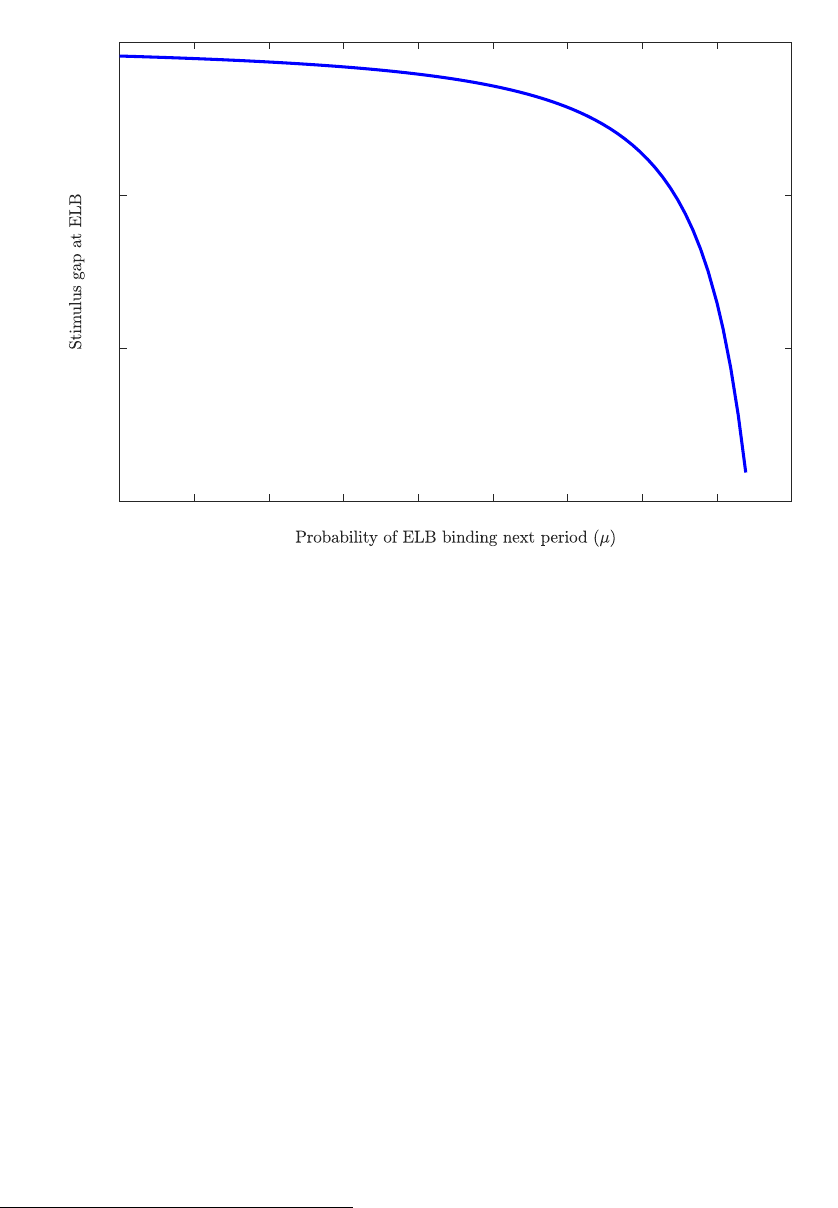
Figure 2: Fiscal stimulus gap at the ELB. Diﬀerence of optimal increase of government

consumption without and with coordination, measured in percentage points along the vertical

axis (ˆg

∗,Nash

− ˆg

∗,Coord

), horizontal axis measures probability that the ELB remains binding

for another period (µ).

−4% (annualized) for the ELB scenario. For all experiments we verify that the ELB remains

binding also as government spending is raised in response to the shock. Table 1 summarizes

the parameter values.

Given these parameter values, we solve the model in the absence of coordination numerically

as in Soderlind (1999). Appendix H provides details. As in our analysis above, we focus on

the ELB scenario and, in particular, on the optimal adjustment of government spending. In

the case of coordination, Proposition 1 provides an analytic solution. Figure 2 displays the

ﬁscal stimulus gap at the ELB: the diﬀerence of the optimal increase of government spending

without and with coordination. Speciﬁcally, the vertical axis measures the diﬀerence of the

percentage change of government spending in percentage points (ˆg

∗,Nash

− ˆg

∗,Coord

). The

horizontal axis measures the probability µ that the ELB remains binding for another period.

The ﬁgure illustrates that whether ﬁscal policies are coordinated or not hardly matters if the

We restrict the range of µ to values for which we obtain a locally unique equilibrium.

0.9 0.92 0.94 0.96 0.98 1

-15

-10

-5

0 2 4 6 8

-15

-10

-5

0 0.2 0.4 0.6 0.8 1

-10

-8

-6

-4

-2

0 0.2 0.4 0.6 0.8 1

-25

-20

-15

-10

-5

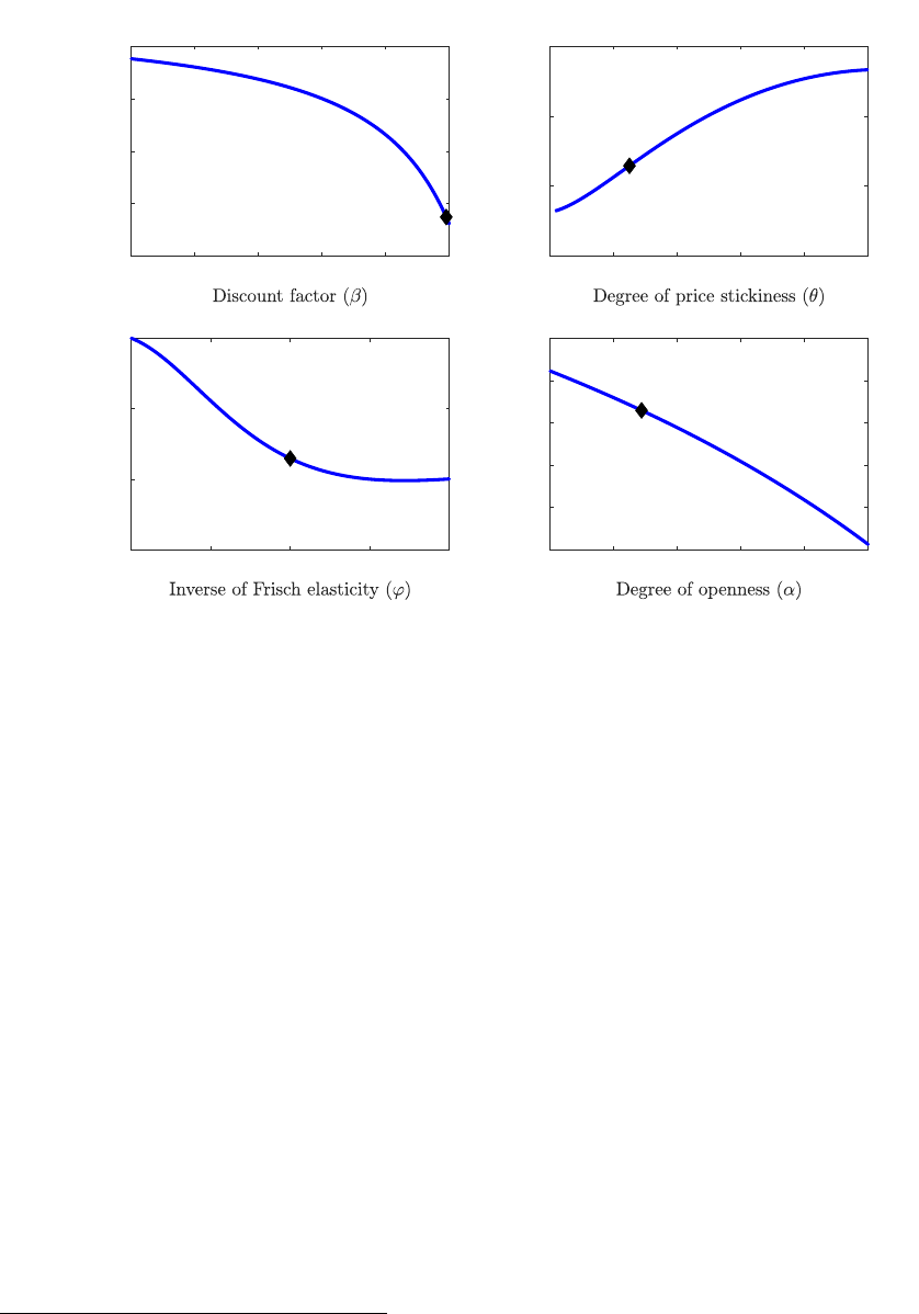
Figure 3: Stimulus gap conditional on the discount factor β (upper-left panel), the degree

of price stickiness (upper-right panel), the inverse of the Frisch elasticity of labor supply ϕ

(lower-left panel) and openness α (lower-right panel) for µ = 0.8, see Figure 2. We only

consider parameter values for which the equilibrium is locally unique. A diamond indicates

parameter values under the baseline parameterization.

expected duration of the ELB episode is short. However, for larger values of µ the stimulus

gap is sizable. If, for instance, the expected duration is ﬁve quarters (µ = 0.8), the diﬀerence

amounts to 8.5 percentage points.

We now illustrate to what extent this result depends on speciﬁc parameter values. For this

purpose we vary one parameter at a time, while keeping µ ﬁxed at 0.8 throughout. We

ﬁrst consider alternative values for the discount factor β. It determines how the dynamics

of the terms of trade (as endogenous state variable) impact optimal policy in the absence

of coordination (see the discussion in Section 3.2 above).

The upper-left panel of Figure

3 shows the stimulus gap as a function of β. We ﬁnd that the stimulus gap increases as β

increases or, put diﬀerently, the desire to avoid a persistent appreciation of the terms of trade

increases with β in the absence of coordination.

At the same time β matters also for the slope of the Phillips curve. Yet, as we vary the value of β, we keep

κ constant (just like all other parameters) in order to focus on the role of the dynamic terms of trade eﬀect.

The upper-right panel of Figure 3 shows the stimulus gap as a function of the degree of price

stickiness θ. We ﬁnd that the lower the degree of price stickiness, the larger the gap between

the optimal policy under coordination and Nash. To understand this ﬁnding, note that

inﬂation responds more strongly to higher government spending if prices are more ﬂexible.

Higher inﬂation at the union level reduces real interest rates and thus stimulates aggregate

demand at the union level. At the country level, instead, higher inﬂation appreciates the

terms of trade and thus reduces the demand for domestically produced goods. Hence, the

more ﬂexible prices, the more negative the stimulus gap.

The lower-left panel of Figure 3 shows the stimulus gap conditional on the inverse of the

Frisch elasticity of labor supply ϕ. As the Frisch elasticity declines (that is, as ϕ increases),

marginal costs and, hence, inﬂation respond more strongly to higher government spending.

Put diﬀerently, the Phillips curve becomes steeper as ϕ increases, just like when θ declines,

see equation (6). We therefore ﬁnd the stimulus gap more negative, the larger the Frisch

elasticity.

The lower-right panel of Figure 3 shows the stimulus gap conditional on openness parameter

α. It is possible to show that, the higher the degree of openness, the stronger the impact of

government spending on the terms of trade. Consequently, in a more open economy policy

makers seek to avoid a stronger appreciation of the terms of trade in the midst of a severe

recession and provide a lower stimulus in the absence of policy coordination. Note that the

stimulus gap does not vanish in the closed economy limit (α = 0) since monetary regimes

still diﬀer. While there is an implicit price-level target in place at the country-level, the price

level features a unit root at the union level. This diﬀerence has a strong bearing on the

transmission of ﬁscal policy (Corsetti et al., 2013b).

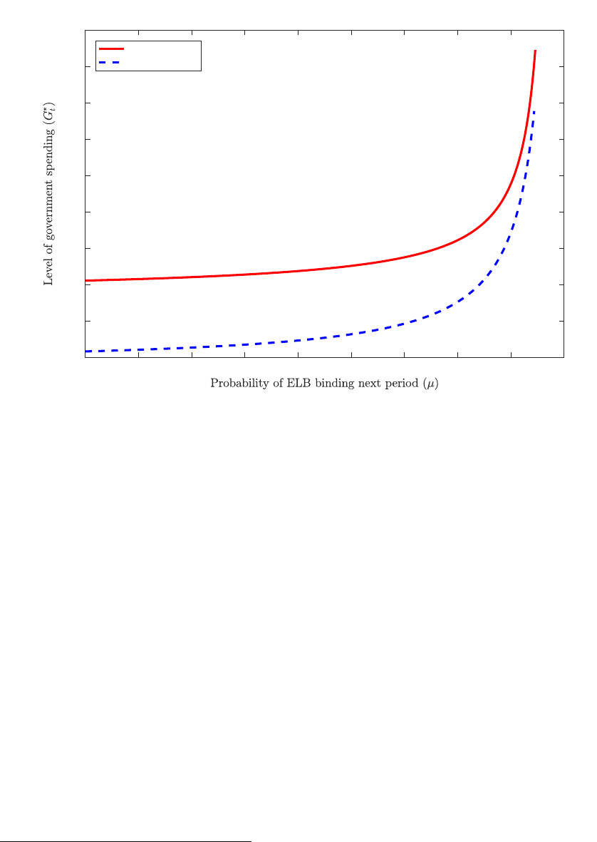
So far we have focused on the stimulus gap, that is for a given steady state we have computed

the percentage point diﬀerence in the optimal variation of government spending with and

without coordination. We have illustrated that the gap can be sizable. However, in Section

3.1 we have established that the level of government spending is too high to begin with

in steady state in the absence of coordination. We therefore compute the optimal level of

government spending in the ELB scenario to see which of these eﬀects dominates and report

results in Figure 4. The vertical axis measures the optimal level of government consumption

with (dashed lines) and without (solid lines) coordination. Along the horizontal axis we

measure again the expected duration of the ELB episode. Results are based on the parameter

values listed in Table 1 above. In this case, we ﬁnd that the steady-state eﬀect dominates:

the level of spending without coordination exceeds the optimal level with coordination for all

0 0.1 0.2 0.3 0.4 0.5 0.6 0.7 0.8 0.9

0.15

0.16

0.17

0.18

0.19

0.2

0.21

0.22

0.23

0.24

w/o coordination

coordination

Figure 4: The optimal level of government spending under coordination (dashed lines) and

without (solid lines) (i.e. G

Coord

and G

Nash

). We only compute results for combinations of

parameters which give rise to a locally unique equilibrium.

values of µ for which we obtain a unique equilibrium.

Nevertheless, the distance between

the optimal level of government expenditure with and without coordination becomes smaller.

Against this background, one may conjecture that there is little need to coordinate on ﬁscal

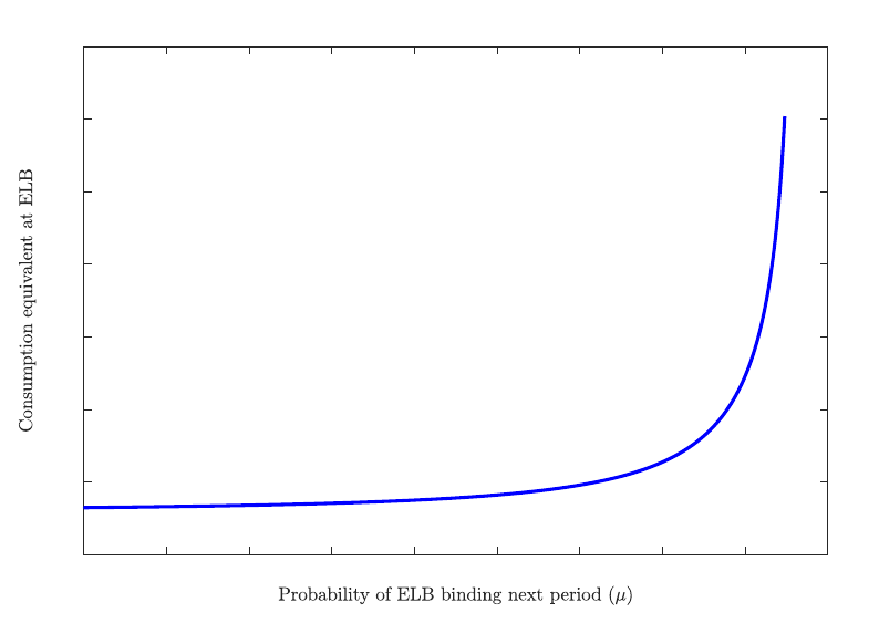
stimulus at the ELB. In order to assess this conjecture formally, we evaluate welfare under

the optimal policy with and without coordination. Speciﬁcally, we compute the consumption

equivalent ζ which compensates the household for the lack of coordination (see Appendix

I for details). Figure 5 displays the result. The vertical axis measures the consumption

equivalent in percentage points of steady-state consumption in the absence of coordination.

The horizontal axis measures the probability µ that the ELB remains binding for another

period. The longer the ELB is expected to bind, the higher the consumption equivalent.

Hence, the need for coordination increases in the duration of the ELB—despite the fact that

the distance between the optimal level of spending shrinks as µ increases (see Figure 4). This

In principle, it is possible that the optimal level of spending without coordination falls short of the optimal

level with coordination. For instance, assuming ϕ = 0.2 and θ = 0.5 we ﬁnd this to be the case, provided the

ELB episode is expected to be suﬃciently long lasting.

0 0.1 0.2 0.3 0.4 0.5 0.6 0.7 0.8 0.9

1.75

1.8

1.85

1.9

1.95

2.05

2.1

Figure 5: Welfare loss due to lack of coordination. Consumption equivalent which compen-

sates for the lack of coordination expressed in percentage points of steady state consumption

in the absence of coordination (see Appendix I).

is because the deviations from the optimal allocation become more costly, the further away

the economy moves from the steady-state under coordination.

Finally, Figure 5 also shows that the largest part of the welfare loss is due to absence of

coordination at steady state (ζ = 1.78 for µ = 0). This is perhaps not surprising since the

economy will return permanently to steady state, once the ELB ceases to bind. Still, when

the expected duration of the ELB is 5 quarters (µ = 0.8) about 15% of the consumption

equivalent are due to lack of coordination at the ELB. This strikes us as sizable, given the

rather short duration of the ELB scenario.

5 Conclusion

In the context of the global ﬁnancial crisis ﬁscal policy has been rediscovered as a stabilization

tool. A central concern in this regard is that monetary policy may become constrained by the

ELB on nominal interest rates precisely at times when the need for stabilization is particularly

large. In this case it not only seems natural to turn to ﬁscal policy for additional support,

it has also been documented that ﬁscal policy is likely to be particularly eﬀective under such

circumstances.

Against this background, we consider a currency union where a common monetary policy

operates jointly with many ﬁscal policies. Assuming that the common monetary policy is

unable to stabilize area-wide inﬂation and output, we ask whether there is a need to coor-

dinate government spending policies across the member states of the union. This possibility

arises because uncoordinated ﬁscal policies induce movements of the terms of trade which are

internalized by a coordinated policy response.

Our analysis is based on the model of Gal´ı and Monacelli (2008) which we extend in order

to account for the ELB and the absence of ﬁscal policy coordination. Absent coordination,

we ﬁnd—in line with earlier results—that each country seeks to improve its terms of trade as

long as the ELB is not binding. In a symmetric equilibrium, however, the terms of trade are

unchanged and government spending is too high relative to the outcome under coordination.

At the ELB, instead, we ﬁnd that the optimal ﬁscal response implies too little ﬁscal stimulus

in the absence of coordination. In this case governments seek to avoid an appreciation of the

terms of trade in order to prevent a loss of competitiveness in times of economic slack.

Hence, absent coordination, the terms-of-trade externality has a diﬀerential impact on the

optimal level of government spending depending on whether the ELB binds or not. Accounting

for both dimensions, we ﬁnd that the welfare loss due to the lack of coordination increases

in the expected duration of the ELB episode. We thus conclude that there is indeed a case

for coordinating ﬁscal stabilization policies in a currency union, once monetary policy is

constrained by an ELB.

References

Acconcia, A., Corsetti, G., and Simonelli, S. (2014). Maﬁa and public spending: Evidence on

the ﬁscal multiplier from a quasi-experiment. American Economic Review, 104(7):2185–

2209.

Beetsma, R. and Jensen, H. (2005). Monetary and ﬁscal policy interactions in a micro-founded

model of a monetary union. Journal of International Economics, (67):320–352.

Beetsma, R. and Uhlig, H. (1999). An analysis of the stability and growth pact. Economic

Journal, (109):546–571.

Beetsma, R. M. W. J. and Bovenberg, A. L. (1998). Monetary union without ﬁscal coordi-

nation may discipline policymakers. Journal of International Economics, 45(2):239–258.

Benigno, G. and Benigno, P. (2003). Price Stability in Open Economies. Review of Economic

Studies, 70(4):743–764.

Benigno, P. (2004). Optimal monetary policy in a currency area. Journal of International

Economics, 63(2):293 – 320.

Benigno, P. and Woodford, M. (2006). Optimal taxation in an RBC model: A linear-quadratic

approach. Journal of Economic Dynamics and Control, 30(9-10):1445–1489.

Blanchard, O., Erceg, C., and Lind, J. (2016). Jump-Starting the Euro Area Recovery: Would

a Rise in Core Fiscal Spending Help the Periphery? In NBER Macroeconomics Annual

2016, Volume 31, NBER Chapters. National Bureau of Economic Research, Inc.

Born, B., Juessen, F., and M¨uller, G. J. (2013). Exchange rate regimes and ﬁscal multipliers.

Journal of Economic Dynamics and Control, 37(2):446–465.

Calvo, G. A. (1983). Staggered prices in a utility-maximizing framework. Journal of Monetary

Economics, 12(3):383 – 398.

Chetty, R., Guren, A., Manoli, D., and Weber, A. (2011). Are micro and macro labor

supply elasticities consistent? a review of evidence on the intensive and extensive margins.

American Economic Review, 101(3):471–75.

Christiano, L., Eichenbaum, M., and Rebelo, S. (2011). When Is the Government Spending

Multiplier Large? Journal of Political Economy, 119(1):78 – 121.

Cook, D. and Devereux, M. B. (2011). Optimal ﬁscal policy in a world liquidity trap. European

Economic Review, 55(4):443–462.

Corsetti, G., Kuester, K., Meier, A., and M¨uller, G. J. (2013a). Sovereign risk, ﬁscal policy,

and macroeconomic stability. The Economic Journal, 123(566):F99–F132.

Corsetti, G., Kuester, K., and M¨uller, G. (2013b). Floats, pegs and the transmission of ﬁscal

policy., volume 17 of Fiscal Policy and Macroeconomic Performance, Central Banking,

Analysis, and Economic Policies Book Series, chapter 7, pages 235–281. in C´espedes, L.F.

and J. Gal´ı (eds.), Santiago, Chile, Central Bank of Chile.

Corsetti, G., Meier, A., Kuester, K., and M¨uller, G. J. (2014). Sovereign risk and belief-driven

ﬂuctuations in the euro area. Journal of Monetary Economics, (61):53–73.

Corsetti, G. and Pesenti, P. (2001). Welfare And Macroeconomic Interdependence. The

Quarterly Journal of Economics, 116(2):421–445.

Cotarelli, C. (2012). Fiscal adjustment: Too much of a good thing? Vox EU.

C´urdia, V. and Woodford, M. (2011). The Central-Bank Balance Sheet as an Instrument of

Monetary Policy. Journal of Monetary Economics, (58):54–79.

C´urdia, V. and Woodford, M. (2015). Credit frictions and optimal monetary policy. Journal

of Monetary Economics, forthcoming.

Cwik, T. and Wieland, V. (2011). Keynesian Government Spending Multipliers and Spillovers

in the Euro Area. Economic Policy, (26):493–549.

De Paoli, B. (2009). Monetary policy and welfare in a small open economy. Journal of

International Economics, 77(1):11–22.

Devereux, M. B. (1991). The terms of trade and the international coordination of ﬁscal policy.

Econmic Inquiry, (102(3)):720–736.

Dixit, A. and Lambertini, L. (2001). Monetary-ﬁscal policy interactions and commitment

versus discretion in a monetary union. European Economic Review, 45(4-6):977–987.

Dixit, A. and Lambertini, L. (2003). Symbiosis of monetary and ﬁscal policies in a monetary

union. Journal of International Economics, 60(2):235–247.

Eggertsson, G. B. and Woodford, M. (2003). The Zero Interest-Rate Bound and Optimal

Monetary Policy. Brookings Papers on Economic Activity, 1:139–211.

Epifani, P. and Gancia, G. (2009). Openness, government size and the terms of trade. The

Review of Economic Studies, 76(2):629–668.

Erceg, C. J. and Lind´e, J. (2012). Fiscal Consolidation in an Open Economy. American

Economic Review, (102(3)):186–191.

Erceg, C. J. and Lind´e, J. (2014). Is There A Fiscal Free Lunch In A Liquidity Trap? Journal

of the European Economic Association, 12(1):73–107.

Evers, M. P. (2015). Fiscal federalism and monetary unions: A quantitative assessment.

Journal of International Economics, 97(1):59–75.

Fahri, E. and Werning, I. (2016). Fiscal Multipliers: Liquidity traps and currency unions.

In Taylor, J. B. and Uhlig, H., editors, Handbook of Macroeconomics, chapter 31, pages

2417–2491. Elsevier.

Forlati, C. (2009). Optimal monetary and ﬁscal policy in the emu: Does ﬁscal policy coor-

dination matter? Center for Fiscal Policy, EPFL, Chair of International Finance (CFI)

Working Paper, (2009-04).

Forlati, C. (2015). On the beneﬁts of a monetary union: Does it pay to be bigger? Journal

of International Economics, 97(2):448–463.

Gal´ı, J. (2008). Monetary policy, inﬂation, and the business cycle. Princeton Univ. Press.

Gal´ı, J. and Monacelli, T. (2005). Optimal Monetary and Fiscal Policy in a Currency Union.

Working Papers 300, IGIER (Innocenzo Gasparini Institute for Economic Research), Boc-

coni University.

Gal´ı, J. and Monacelli, T. (2008). Optimal monetary and ﬁscal policy in a currency union.

Journal of International Economics, 76(1):116 – 132.

Gal´ı, J. and Monacelli, T. (2015). A Note on Martin Hellwig’s “The Gal´ı-Monacelli Model of

a Small Open Economy Has No International Trade”. mimeo.

Giannoni, M., Patterson, C., and Negro, M. D. (2016). The Forward Guidance Puzzle.

Technical report.

Groll, D. and Monacelli, T. (2016). The Inherent Beneﬁt of Monetary Unions. CEPR Dis-

cussion Papers 11416, C.E.P.R. Discussion Papers.

Hellwig, M. (2015). The Gal´ı-Monacelli Model of a Small Open Economy Has No International

Trade. mimeo.

Kirsanova, T., Satchi, M., Vines, D., and Wren-Lewis, S. (2007). Optimal Fiscal Policy Rules

in a Monetary Union. Journal of Money, Credit and Banking, 39(7):1759–1784.

Krogstrup, S. and Wyplosz, C. (2010). A common pool theory of supranational deﬁcit ceilings.

European Economic Review, 54:273–282.

Krugman, P. (2008). The economic consequences of Herr Steinbrueck. New York Times.

Nakamura, E. and Steinsson, J. (2014). Fiscal stimulus in a monetary union: Evidence from

us regions. American Economic Review, 104(3):753–92.

Pappa, E. (2004). Do the {ECB} and the fed really need to cooperate? optimal monetary

policy in a two-country world. Journal of Monetary Economics, 51(4):753 – 779.

Rogoﬀ, K. S. (2016). The Curse of Cash. Princeton University Press.

Schmidt, S. (2013). Optimal Monetary and Fiscal Policy with a Zero Bound on Nominal

Interest Rates. Journal of Money, Credit and Banking, 45(7):1335–1350.

Schmidt, S. (2016). Fiscal activism and the zero nominal interest rate bound. Journal of

Money, Credit and Banking, forthcoming.

Soderlind, P. (1999). Solution and estimation of RE macromodels with optimal policy. Eu-

ropean Economic Review, 43(4-6):813–823.

Svensson, L. E. O. (1997). Optimal inﬂation targets, ”conservative” central banks, and linear

inﬂation contracts. The American Economic Review, 87(1):98–114.

Turnovsky, S. J. (1988). The gains from ﬁscal cooperation in the two-commodity real trade

model. Journal of International Economics, 25(1-2):111–127.

Woodford, M. (2011). Simple analytics of the government expenditure multiplier. American

Economic Journal: Macroeconomics, 3(1):1 – 35.

A Steady state under coordination

Note that the risk sharing condition and the market-clearing condition in (15) imply

= (Y

− G

)

1−α

∗

)

. (A.1)

The Lagrangian associated with problem (15) is given by

L =

(1 − χ) log C

+ χ log G

−





1+ϕ

1 + ϕ

− (N

− G

)

1−α

∗

)

)di − µ



∗

−



First order conditions are given by:

∂L

∂C

= (1 − χ)

+ Λ

+ µ = 0 (A.2)

∂L

∂C

∗

= Λ

α(N

− G

)

1−α

∗

)

α−1

− µ = 0 (A.3)

∂L

∂N

= −(N

)

− Λ

(1 − α)(N

− G

)

−α

∗

)

= −(N

)

− Λ

(1 − α)

− G

= 0 (A.4)

∂L

∂G

= χ

+ Λ

(1 − α)(N

− G

)

−α

∗

)

= χ

+ Λ

(1 − α)

− G

= 0. (A.5)

Combining (A.2) and (A.3) yields:

(1 − χ)

+ Λ

= −Λ

α(N

− G

)

1−α

∗

)

α−1

. (A.6)

Combining (A.4) and (A.5) gives:

)

= χ

. (A.7)

Further, combining (A.5) and (A.6) gives:

(1 − χ)

− χ

1 − α

− G

= −χ

1 − α

− G

α(N

− G

)

1−α

∗

)

α−1

. (A.8)

One can guess and verify that the solution under coordination, that is, to equations (A.7)

and (A.8) is given by (see Gal´ı and Monacelli, 2008):

= 1 − χ

∗

= 1 − χ

= χ

= N

= 1.

Hence, the steady-state ratio of government spending to output in any given country i ∈ [0, 1]

is given by:

Coord

≡





Coord

= χ,

while output is given by:

Coord

= 1.

B Steady state in the absence of coordination

B.1 Planner problem

The Lagrangian associated with problem (17) is given by

L =(1 − χ) log C

+ χ log G

−





1+ϕ

1 + ϕ

+ Λ(C

− (N

− G

)

1−α

∗

)

First order conditions are given by:

∂L

∂C

= (1 − χ)

+ Λ = 0 (B.9)

∂L

∂N

= −(N

)

− Λ(1 − α)(N

− G

)

−α

∗

)

(A.1)

= −(N

)

− Λ(1 − α)

− G

= 0 (B.10)

∂L

∂G

= χ

+ Λ(1 − α)(N

− G

)

−α

∗

)

= χ

+ Λ(1 − α)

− G

= 0. (B.11)

Combine (B.10) and (B.11) to get:

)

= χ

. (B.12)

Further, combine (B.9) and (B.11):

1 − χ

= (1 − α)

− G

Which can be rearranged to:

1 − χ



(1 − α) +

1 − χ



−1

. (B.13)

It thus follows for the steady state in the absence of coordination (Nash) in any given country

i ∈ [0, 1] that:





Nash

(1 − α)(1 − χ) + χ

. (B.14)

Since in a symmetric steady state Y

= N

, combining (B.12) and (B.14) gives:

Nash

= Y

Nash

= [(1 − α)(1 − χ) + χ]

1+ϕ

. (B.15)

Further, it holds that G

Coord

< G

Nash

since

Coord

= χ <

(1 − α)(1 − χ) + χ

[(1 − α)(1 − χ) + χ]

1+ϕ

= G

Nash

B.2 Decentralization of the planner solution in steady state

In the following we show how the planner allocation in the absence of coordination can be

decentralized in a symmetric zero-inﬂation steady state. Unless oﬀset by the employment

subsidy, ﬁrms choose a constant mark-up over marginal costs MC

, which can be expressed

as (see equation (41) in Gal´ı and Monacelli, 2008):

1 −

= MC

1 − τ

1 − χ

)

1+ϕ



1 −



In order to decentralize the planner solution government consumption, G

, has to follow a

rule according to (B.13). Solving the resulting expression for N

gives:

)

1+ϕ



1 −



1 − χ

1 − τ

1 −

1 − χ



(1 − α) +

1 − χ



−1

By additionally choosing the following subsidy

1 − τ



1 −



(1 − α)

−1

, (B.16)

the social planner solution without coordination is decentralized in a symmetric zero-inﬂation

steady state.

C Deriving the welfare function without coordination

In the absence of coordination there are linear terms in a second-order approximation to

household utility. We follow the approach of Benigno and Woodford (2006) and substitute

for the linear terms using a second order approximation to the market-clearing condition.

In the following we drop the country index i for simplicity and approximate the percentage

deviation of a generic variable X

from its steady state X by

− X

≈ ˆx

ˆx

where ˆx

= x

− x and x

= log X

C.1 Second order approximation to the goods market clearing condition

The market-clearing condition is given by Y

= C

. Taking logs and rearranging gives:

log C

= log(Y

− G

) − α log S

Using the second-order approximation for log(Y

− G

) around a generic steady state from

the appendix in Gal´ı and Monacelli (2008) and noting that a second-order approximation of

log C

and log S

is in fact linear we obtain:

ˆc

≈

1 − γ

(ˆy

− γˆg

) −

(1 − γ)

(ˆg

− ˆy

)

− αs

. (C.17)

Combining the above equation with the risk-sharing condition (3) yields:

0 ≈

1 − γ

(ˆy

− γˆg

) −

(1 − γ)

(ˆg

− ˆy

)

− s

+ t.i.p. (C.18)

where (t.i.p.) captures terms independent of policy. This includes ˆc

∗

since it evolves exoge-

nously for a given member of the currency union. For future reference, we deﬁne:

≡

1 − γ

; A

≡ −

1 − γ

; A

≡ −1. (C.19)

C.2 Second order approximation to utility

Utility U

= U(C

, G

, N

) is additively separable in its arguments. A second order approxi-

mation around a generic steady state C, G, N therefore gives:

− U ≈ U



− C



+ U



− G



+ U



− N





− C





− G





− N



Rewriting the expression in terms of log deviations the above approximation becomes:

− U ≈ U



ˆc



+ U



ˆg



+ U



ˆn



ˆc

ˆg

ˆn

Rearranging:

− U ≈ U



ˆc



1 +



ˆc



+ U



ˆg



1 +



ˆg



+ U



ˆn



1 +



ˆn



Deﬁning further: σ ≡ −

, σ

≡ −

and σ

≡

yields

− U ≈ U



ˆc

(1 − σ) ˆc



+ U



ˆg

(1 − σ

) ˆg



+ U



ˆn

(1 + σ

) ˆn



Since utility is given by

= (1 − χ) log C

+ χ log G

−

1+ϕ

1 + ϕ

the above deﬁned parameters become: σ = σ

= 1 while σ

= ϕ, such that we get:

− U

≈ ˆc

ˆg



ˆn

(1 + ϕ)ˆn



Because of monopolistic competition ﬁrms charge a markup over marginal costs. If not oﬀset

by a certain value for the labor subsidy there will be a wedge Φ between the marginal rate

of substitution and the marginal product of labor (MPN) in steady state (see, for instance,

Gal´ı, 2008, p.106):

−

= MPN(1 − Φ). (C.20)

In our setup we have MPN = Y/N. Therefore

= −

1 − γ

(1 − Φ),

with 1 − γ = C/Y . Making use of the above expression and the one for

under the

assumed utility function, we can rewrite the approximation to utility as:

− U

≈ ˆc

1 − χ

ˆg

−

1 − Φ

1 − γ



ˆn

(1 + ϕ)ˆn



Further, we use equation (C.17) in order to substitute for ˆc

. Therefore

− U

≈

1 − γ

(ˆy

− γˆg

) −

(1 − γ)

(ˆg

− ˆy

)

− αs

1 − χ

ˆg

−

1 − Φ

1 − γ



ˆn

(1 + ϕ)ˆn



In order to substitute for ˆn

, it can be shown that aggregate labor demand is given by

= Y



(j)



−ε

dj, see Gal´ı and Monacelli (2008). Deﬁne z

≡ log



(j)



−ε

dj. Thus,

it holds around a symmetric steady state that:

ˆn

= ˆy

+ z

Further it can be shown that z

is of second order with z

≈

, see again Gal´ı and

Monacelli (2008). Finally, the approximation to utility can be expressed as:

− U

≈

1 − γ

ˆy



1 − χ

−

1 − γ



ˆg

− αs

−

(1 − γ)

(ˆg

− ˆy

)

−

1 − Φ

1 − γ

(1 + ϕ)ˆy

−

1 − Φ

1 − γ

. (C.21)

Deﬁne:

≡

1 − γ

; B

≡

1 − χ

−

1 − γ

; B

≡ −α. (C.22)

Note that the welfare function under coordination can be obtained from (C.21) if one ap-

proximates around the eﬃcient steady state from the union wide perspective. In that steady

state the labor subsidy is chosen such that Φ = 0 and γ equals χ since government spending

is chosen eﬃciently. The terms of trade drop out by computing union-wide welfare, that is

by taking the integral of (C.21) over all i ∈ [0, 1].

C.3 The welfare function—substituting for the linear terms

Absent coordination, government spending and the employment subsidy, τ, are not chosen

eﬃciently such that γ = γ

Nash

6= χ and Φ 6= 0. Speciﬁcally, in a symmetric steady state the

distortion Φ is given by (see Gal´ı, 2008, p.73 and p.106):

Φ = 1 −

ε−1

(1 − τ )

Inserting for the subsidy according to (B.16) yields:

Φ = α.

By inserting for γ

Nash

and Φ in (C.19) and (C.22) we get:

(1 − χ)(1 − α) + χ

(1 − χ)(1 − α)

; A

= −

(1 − χ)(1 − α)

; A

= −1;

α[(1 − χ)(1 − α) + χ]

(1 − χ)(1 − α)

; B

= −

αχ

(1 − χ)(1 − α)

; B

= −α.

Thus, it is easily seen that subtracting α times condition (C.18) from (C.21)—both evaluated

at the Nash steady state—removes the linear terms from the approximation to utility. As a

result, the welfare function is given by:

Nash

≈ −



(π

)

+ (1 + ϕ)(ˆy

)

Nash

1 − γ

Nash



ˆg

− ˆy





+ t.i.p.

D Optimal policy with coordination

The Lagrangian associated with problem (19) is given by

= −



(π

∗

)

+ (1 + ϕ)(ˆy

∗

)

Coord

1 − γ

Coord

(ˆg

∗

− ˆy

∗

)



+ ξ

∗

0,t



∗

− λ



1 − γ

Coord

+ ϕ



ˆy

∗

λγ

Coord

1 − γ

Coord

ˆg

∗

− ν

∗

0,t



+ ξ

∗

1,t



−(ˆy

∗

− γˆg

∗

) + ν

∗

1,t



The Kuhn-Tucker conditions read as follows:

∂L

∂π

∗

= −

∗

+ ξ

∗

0,t

= 0 (D.23)

∂L

∂ˆy

∗

= −(1 + ϕ)ˆy

∗

Coord

1 − γ

Coord

(ˆg

∗

− ˆy

∗

) − λ



1 − γ

Coord

+ ϕ



∗

0,t

− ξ

∗

1,t

= 0 (D.24)

∂L

∂ˆg

∗

= −

Coord

1 − γ

Coord

(ˆg

∗

− ˆy

∗

) +

λγ

Coord

1 − γ

Coord

∗

0,t

+ γ

Coord

∗

1,t

= 0 (D.25)

∗

1,t

(−(ˆy

∗

− γˆg

∗

) + ν

∗

1,t

) = 0

∗

1,t

≥ 0; −(ˆy

∗

− γˆg

∗

) + ν

∗

1,t

≥ 0.

Case 1 The eﬀective-lower-bound constraint does not bind: ξ

∗

1,t

= 0 and −(ˆy

∗

−γˆg

∗

)+ν

∗

1,t

≥

0. Equation (D.25) thus implies for ξ

∗

0,t

∗

0,t

(ˆg

∗

− ˆy

∗

). (D.26)

Inserting for ξ

∗

0,t

in (D.24) yields

0 = −(1 + ϕ)ˆy

∗

Coord

1 − γ

Coord

(ˆg

∗

− ˆy

∗

) − λ



1 − γ

Coord

+ ϕ



(ˆg

∗

− ˆy

∗

)

0 = −(1 + ϕ)ˆy

∗

− (1 + ϕ)(ˆg

∗

− ˆy

∗

)

ˆg

∗

= 0.

Thus by (D.26)

∗

0,t

= −

ˆy

∗

. (D.27)

Combining (D.27) and (D.23):

ˆy

∗

= −επ

∗

Therefore, when it is optimal to stabilize output at steady state inﬂation should be zero and

vice versa. And indeed, considering the functional form of the welfare function it is clear that

∗

= ˆy

∗

= ˆg

∗

= 0 is the global maximum.

Case 2 The eﬀective-lower-bound constraint binds: ξ

∗

1,t

> 0 and −(ˆy

∗

− γˆg

∗

) + ν

∗

1,t

= 0.

Rearrange (D.25):

−ξ

∗

1,t

= −

1 − γ

Coord

(ˆg

∗

− ˆy

∗

) +

1 − γ

Coord

∗

0,t

. (D.28)

Combining it with (D.24):

0 = −(1 + ϕ)ˆy

∗

Coord

1 − γ

Coord

(ˆg

∗

− ˆy

∗

) − λ



1 − γ

Coord

+ ϕ



∗

0,t

−

1 − γ

Coord

(ˆg

∗

− ˆy

∗

) +

1 − γ

Coord

∗

0,t

∗

0,t

= −

ˆy

∗

−

λϕ

ˆg

∗

. (D.29)

Inserting for ξ

∗

0,t

in (D.23) yields after rearranging

∗

ˆy

∗

= −ψ

Coord

ˆg

∗

, (D.30)

where ψ

Coord

≡

εϕ

E Optimal policy in the absence of coordination

The Lagrangian associated with problem (21) is given by

= −



(π

)

+ (1 + ϕ)(ˆy

)

1 − γ



ˆg

− ˆy





+ βE

V (s

, π

∗

t+1

, ˆc

∗

t+1

)

+ m

1,t



ˆy

− γˆg

− (1 − γ)ˆc

∗

− (1 − γ)s



+ m

2,t



− βE

t+1

− λ



1 − γ

+ ϕ



ˆy

+ λ

1 − γ

ˆg



+ m

3,t



− π

∗

+ s

− s

t−1



and E

t+1

given.

Note that while E

t+1

is taken as given, it is a given function of today’s state variable s

First order conditions

∂L

∂π

= −

+ m

2,t

+ m

3,t

= 0 (E.31)

∂L

∂ˆy

= −(1 + ϕ)ˆy

1 − γ

(ˆg

− ˆy

) + m

1,t

− λ



1 − γ

+ ϕ



2,t

= 0 (E.32)

∂L

∂ˆg

= −

1 − γ

(ˆg

− ˆy

) − γm

1,t

λγ

1 − γ

2,t

= 0 (E.33)

∂L

∂s

= βE

∂V

∂s

− (1 − γ)m

1,t

− m

2,t

β∂E

t+1

∂s

+ m

3,t

= 0. (E.34)

Solving ﬁrst order conditions (E.32) and (E.33) for m

2,t

yields

2,t

= −

ˆy

−

λϕ

ˆg

This implies for m

3,t

by (E.31)

ˆy

λϕ

ˆg

First order condition (E.33) thus requires for m

1,t

that

1,t

= −

1 − γ

(ˆg

− ˆy

) −

1 − γ

ˆy

−

1 − γ

ˆg

Finally, substituting for the multipliers in (E.34) gives

− λβE

∂V

∂s

+ β



ˆy

ˆg



∂E

t+1

∂s

ˆy

+ π

= −ψ

Nash

ˆg

with ψ

Nash

≡

εϕ

(λϕ + (1 + λ)). Taking the limit of β → 0 the above condition becomes

ˆy

+ π

= −ψ

Nash

ˆg

. (E.35)

F Proof of Proposition 1

In Proposition 1 we state the solution for optimal government consumption at the ZLB with

coordination. We prove the proposition more generally in order to use results for the proof

of proposition 2. That is, we index regime dependent parameters by j ∈ {Coord, Nash}.

Optimal policy at the ELB is determined by equations (12), (14) and (D.30) or (E.35) re-

spectively. The equations are repeated here for convenience:

∗,j

1 − βµ

(ˆy

∗,j

−

¯σ

+ ϕ

ˆg

∗,j

) (F.36)

ˆy

∗,j

(1 − γ

)(1 − βµ)

(1 − µ)(1 − βµ) − (1 − γ

)µκ

(1 − µ)(1 − βµ)γ

− (1 − γ

)µκ

¯σ

+ϕ

(1 − µ)(1 − βµ) − (1 − γ

)µκ

ˆg

∗,j

(F.37)

0 = π

∗,j

ˆy

∗,j

+ ψ

ˆg

∗,j

. (F.38)

Equations (F.36) and (F.38) imply:

−

ˆy

∗,j

− ψ

ˆg

∗,j

1 − βµ

(ˆy

∗,j

−

¯σ

+ ϕ

ˆg

∗,j

Making use of

¯σ

+ϕ

λγ

1−γ

, the above equation can be rearranged to:

ˆy

∗,j

ελγ

1−γ

− (1 − βµ)εψ

ε + (1 − βµ)

ˆg

∗,j

. (F.39)

Combining (F.37) and (F.39), making use of

¯σ

+ϕ

λγ

1−γ

again, yields:

ελγ

1−γ

− (1 − βµ)εψ

ε + (1 − βµ)

ˆg

∗,j

(1 − γ

)(1 − βµ)

(1 − µ)(1 − βµ) − (1 − γ

)µκ

(1 − µ)(1 − βµ)γ

− µλγ

(1 − µ)(1 − βµ) − (1 − γ

)µκ

ˆg

∗,j

Solving for ˆg

∗,j

we get:

ˆg

∗,j

= −Θ

with

= −

(1 − γ

)(1 − βµ)

(1 − µ)(1 − βµ) − (1 − γ

)µκ

λγ

1−γ

− (1 − βµ)ψ

ε + (1 − βµ)

−

(1 − µ)(1 − βµ)γ

− µλγ

(1 − µ)(1 − βµ) − (1 − γ

)µκ

−1

After rearranging, we obtain

(1 − γ

)



ε + (1 − βµ)



ε [(1 − µ)(1 − βµ) − (1 − γ

)µκ

] + (1 − µ)γ

λϕε + γ

[(1 − µ)(1 − βµ) − µλ]

(F.40)

which is the expression in the main text. Since we consider only uniquely determined equilibria

(see the ELB scenario in Section 2.2), the ﬁrst term in the denominator is positive. Further,

because λ < (1 − γ

)κ

, also (1 − µ)(1 − βµ) − µλ > 0. All other expressions in Θ

are non-

negative. Hence, Θ

> 0. 

G Proof of Proposition 2

For β → 0 we obtain from (F.40)

(1 − γ

)



ε + 1



ε [(1 − µ) − (1 − γ

)µκ

] + (1 − µ)γ

λϕε + γ

[(1 − µ) − µλ]

Proposition 2 states that for β → 0 it holds that ˆg

∗,Nash

< ˆg

∗,Coord

. Or put diﬀerently that

Nash

< Θ

Coord

. Formally, we have:

(1 − γ

Nash

)



Nash

ε + 1



Nash

ε [(1 − µ) − (1 − γ

Nash

)µκ

Nash

] + (1 − µ)γ

Nash

λϕε + γ

Nash

[(1 − µ) − µλ]

(1 − γ

Coord

)



Coord

ε + 1



Coord

ε [(1 − µ) − (1 − γ

Coord

)µκ

Coord

] + (1 − µ)γ

Coord

λϕε + γ

Coord

[(1 − µ) − µλ]

Since we showed in Appendix F that all terms in Θ

Nash

and Θ

Coord

are non-negative, we

prove the above inequality by showing that the following holds:

Coord



(1 − µ) − (1 − γ

Coord

)µκ

Coord



+ (1 − µ)γ

Coord

λϕε + γ

Coord

[(1 − µ) − µλ]

Nash



(1 − µ) − (1 − γ

Nash

)µκ

Nash



+ (1 − µ)γ

Nash

λϕε + γ

Nash

[(1 − µ) − µλ]

< 1 <

(1 − γ

Coord

)



Coord

ε + 1



(1 − γ

Nash

)



Nash

ε + 1



(G.41)

We start with the left hand side of (G.41):

Coord



(1 − µ) − (1 − γ

Coord

)µκ

Coord



+ (1 − µ)γ

Coord

λϕε + γ

Coord

[(1 − µ) − µλ]

Nash

ε [(1 − µ) − (1 − γ

Nash

)µκ

Nash

] + (1 − µ)γ

Nash

λϕε + γ

Nash

[(1 − µ) − µλ]

< 1,

which can be rearranged to:

0 <(ψ

Nash

− ψ

Coord

)(1 − µ)ε

− ψ

Nash

(1 − γ

Nash

)εµκ

Nash

+ ψ

Coord

(1 − γ

Coord

)εµκ

Coord

+ (γ

Nash

− γ

Coord

)(1 − µ)λϕε + (γ

Nash

− γ

Coord

) [(1 − µ) − µλ] .

Inserting for ψ

and κ

with j ∈ {Coord, Nash} yields after rearranging:

0 <

λ(1 + ϕ)(1 − µ)

−

(1 + λ(1 + ϕ))µλ



1 + (1 − γ

Nash

)ϕ



µλ



1 + (1 − γ

Coord

)ϕ



+ (γ

Nash

− γ

Coord

)(1 − µ)λϕε + (γ

Nash

− γ

Coord

) [(1 − µ) − µλ] .

This inequality can be further rearranged to:

0 <

λ(1 + ϕ)



(1 − µ) − (1 − γ

Nash

)µκ

Nash



| {z }

+ (γ

Nash

− γ

Coord

)

| {z }

(1 − µ)(λϕε + 1),

where the sign of the highlighted terms follows from the condition on the uniqueness of

equilibrium (see also Appendix F) and the relationship between the steady states with and

without coordination. Hence, we have established that the left hand side is below unity.

We continue with the right hand side of (G.41) which— making use of the deﬁnition of κ—can

be rearranged to:

(1 − γ

Coord

)



λ(

1 − γ

Coord

+ ϕ)ε + 1



> (1 − γ

Nash

)



λ(

1 − γ

Nash

+ ϕ)ε + 1



The above expression can be further rearranged to:

(γ

Nash

− γ

Coord

)(λϕε + 1) > 0,

which holds true since γ

Nash

> γ

Coord

while the remaining parameters are positive. 

H Numerical solution

In order to solve the model numerically we use the algorithm put forward by Soderlind (1999).

The equilibrium conditions are cast in the following form:

1t+1

2t+1

= A

+ Bu

t+1

×1

. (H.42)

In the expression above x

are predetermined variables and x

are non-predetermined vari-

ables. The policy instrument is denoted by u

and ε

t+1

are innovations to x

. Under discretion

the policy problem is given in general terms by the following expression:

V x

+ v

= min



+ 2x

+ u

+ βE

1t+1

V x

1t+1

+ v

t+1

}



(H.43)

s.t. E

2t+1

= Cx

1t+1

, Eq. (H.42), and x

given,

where x

V x

is the value function (quadratic in the state variables), x

+2x

the period loss function and x

= Cx

maps predetermined variables into non-predetermined

variables.

Equations (4), (6) and (7) can be cast into this setup by rewriting them as follows:

{π

t+1

} =

(1 + κ(1 − γ)) π



1 − γ

− κ



ˆg

−

κ(1 − γ)(ˆc

∗

+ π

∗

+ s

t−1

)

= π

∗

− π

+ s

t−1

The vectors in (H.42) are thus given by







t−1

∗

ˆc

∗







, x

, u

= ˆg

, ε







∗

ˆc

∗







, x







t−1

∗

ˆc

∗







where x

is introduced for notational convenience. Matrices A and B are given by

A =







1 1 0 −1

0 0 0 0

−

κ(1 − γ) −

κ(1 − γ)

(1 + κ(1 − γ))







, B =









1−γ

− κ









We multiply the period loss function by 2 and rearrange it to

(π

)



(1 + ϕ) +

Coord

1 − γ

Coord



(ˆy

)

− 2

Coord

1 − γ

Coord

ˆy

ˆg

Coord

1 − γ

Coord

(ˆg

)

This can be written as

ˆy

ˆg







0 0

0 (1 + ϕ) +

Coord

1−γ

Coord

−

Coord

1−γ

Coord

0 −

Coord

1−γ

Coord

1−γ

Coord













ˆy

ˆg







ˆy

ˆg







ˆy

ˆg







We deﬁne the auxiliary matrix K:







ˆy

ˆg













0 0 0 1 0

(1 − γ) (1 − γ) (1 − γ) −(1 − γ) γ

0 0 0 0 1













t−1

∗

ˆc

∗

ˆg







= K

where we make use of

ˆy

= γˆg

+ (1 − γ)ˆc

∗

+ (1 − γ)(π

∗

− π

+ s

t−1

The loss function can therefore be written as

ˆy

ˆg







0 0

0 (1 + ϕ) +

Coord

1−γ

Coord

−

Coord

1−γ

Coord

0 −

Coord

1−γ

Coord

1−γ

Coord













ˆy

ˆg







W K

Therefore, the matrices in (H.43) are given by

Q U

= K

W K.

The solution to (H.43) gives the policy rule (see Soderlind, 1999):

= −F x

Put diﬀerently

ˆg

= −f

t−1

− f

∗

− f

ˆc

∗

In a symmetric equilibrium the terms of trade are zero and the equilibrium is determined at

the union level, see Appendix F. The equilibrium conditions in the ELB scenario are:

ˆg

∗,Nash

= −f

∗,Nash

− f

ˆc

∗,Nash

1 − βµ

κ(ˆy

∗,Nash

−

¯σγ

¯σ + ϕ

ˆg

∗,Nash

)

ˆy

∗,Nash

(1 − γ)(1 − βµ)

(1 − µ)(1 − βµ) − (1 − γ)µκ

(1 − µ)(1 − βµ)γ − (1 − γ)µκ

γ¯σ

¯σ+ϕ

(1 − µ)(1 − βµ) − (1 − γ)µκ

ˆg

∗,Nash

ˆy

∗,Nash

= γˆg

∗,Nash

+ (1 − γ)ˆc

∗,Nash

Given the numerical solution for f

and f

we solve the above system for ˆg

∗,Nash

I Consumption equivalent

We compute the consumption equivalent as the (constant) value that has to be given to the

household in the absence of coordination in order to make her in expected terms as well

oﬀ as under coordination. Below we are more explicit about the exact expression for the

consumption equivalent. We start by computing expected lifetime utility assuming that the

economy is initially at the ELB in period 0. With probability µ the ELB remains binding

and with probability 1 − µ the economy reverts permanently back to steady state. Denote

by U

the utility of the household in a given period at the ELB and by U the utility of the

household in a given period in steady state. The following chart—in which the arrows de-

pict transition probabilities—illustrates how to compute expected discounted lifetime utility

= E

∞

t=0

Expected discounted utility

Period 0: U

↓

1−µ

Period 1: µβU

(1 − µ)βU

↓

1−µ

Period 2: (µβ)

(1 − µ)µβ

U (1 − µ)β

↓

1−µ

Period 3: (µβ)

(1 − µ)µ

U (1 − µ)µβ

U (1 − µ)β

| {z }

(µβ)

(1 − µ)βU

(µβ)

(1 − µ)β

(µβ)

(1 − µ)β

(µβ)

. . .

Therefore, expected discounted lifetime utility can be written as:

= U

∞

t=0

(µβ)

+ (1 − µ)βU

∞

t=0

(µβ)

∞

t=0

, (I.44)

where

= (1 − χ) log C

+ χ log G

−

)

1+ϕ

1 + ϕ

U = (1 − χ) log C + χ log G −

1+ϕ

1 + ϕ

Since µβ < 1 the geometric series in (I.44) converges to:



1 − µβ





1 − µ

1 − µβ



1 − β



The consumption equivalent is a constant compensation that makes the household in the

absence of coordination as well oﬀ as under coordination. More speciﬁcally, the household

receives a compensation ζ such that the following equality holds

Coord

Nash

(ζ), (I.45)

where

Nash

(ζ) =



1 − µβ



Nash

(ζ) +



1 − µ

1 − µβ



1 − β



Nash

(ζ),

with

Nash

(ζ) = (1 − χ) log(C

Nash

(1 + ζ)) + χ log G

Nash

−



Nash



1+ϕ

1 + ϕ

Nash

(ζ) = (1 − χ) log(C

Nash

(1 + ζ)) + χ log G

Nash

−



Nash



1+ϕ

1 + ϕ

Inserting in (I.45) yields:

Coord

1 − µβ

(1 − χ) log(C

Nash

(1 + ζ)) + χ log G

Nash

−



Nash



1+ϕ

1 + ϕ



1 − µ

1 − µβ



1 − β



(1 − χ) log(C

Nash

(1 + ζ)) + χ log G

Nash

−



Nash



1+ϕ

1 + ϕ

Rearranging further

(1 − µβ)

Coord

− U

Nash

(0) − (1 − µ)



1 − β



Nash

(0)

= (1 − χ) log(1 + ζ)



1 + (1 − µ)



1 − β



The above equation can be rearranged to:

ζ = exp

(

1 − χ



1 + (1 − µ)



1 − β



−1



(1 − µβ)

Coor d

− U

N ash

(0) − (1 − µ)



1 − β



N ash

(0)



)

− 1.

We back out G

and Y

from our numerical solution to equations (F.36)-(F.38) making use

of Y = N (which holds in a ﬁrst order approximation). We use the non-linearized version

of (5) to compute C

. The steady state values are obtained from the solution to the social

planner problems.