Polynomial Lyapunov Functions and Invariant Sets from a New
Hierarchy of Quadratic Lyapunov Functions for LTV Systems
Hassan Abdelraouf
1
, Eric Feron
2
, and Jeff S. Shamma
3
Abstract— We introduce a new class of quadratic functions
based on a hierarchy of linear time-varying (LTV) dynamical
systems. These quadratic functions in the higher order space
can be also seen as a non-homogeneous polynomial Lyapunov
functions for the original system, i.e the first system in the
hierarchy. These non-homogeneous polynomials are used to
obtain accurate outer approximation for the reachable set
given the initial condition and less conservative bounds for the
impulse response peak of linear, possibly time-varying systems.
In addition, we pose an extension to the presented approach
to construct invariant sets that are not necessarily Lyapunov
functions. The introduced methods are based on elementary
linear systems theory and offer very much flexibility in defining
arbitrary polynomial Lyapunov functions and invariant sets for
LTV systems.
I. INTRODUCTION
Linear time-varying (LTV) systems appear in many ap-
plications such as changing the aerodynamic coefficients of
the aircraft with the flight speed and altitude or changing the
parameters of chemical plants or electrical circuits. In control
theory, it is common to treat some nonlinear systems as LTV
systems and linear switching systems by local linearization
around a set of operating points [1]. Lyapunov functions are
a widely used concept to tackle stability and related analyses
for linear systems in control literature. For example, the
stability of a linear time-invariant (LTI) system is equivalent
to the existence of a quadratic Lyapunov function. However,
the stability of LTV systems does not necessarily imply the
existence of such a quadratic Lyapunov function, but it is
equivalent to the existence of a polynomial homogeneous
higher order Lyapunov function [2], [3].
Stability and control of switching systems have been
widely studied [4]. In [5], polynomial, homogeneous Lya-
punov functions for uncertain systems is shown to be equiv-
alent to a quadratic Lyapunov function for a transformed
system. Authors in [6], generalized this idea and defined
a hierarchy of dynamical systems using a lifting procedure
such that the quadratic Lyapunov functions for any system
in the hierarchy can be used as a polynomial homogeneous
Lyapunov function for the original system. Then, the search
for homogeneous Lyapunov function for LTV systems can
be recast as the search for a quadratic Lyapunov function in
a related hierarchy. In this paper, we extend the contents of
[6] and add more flexibility to the methods described therein
1
PhD candidate, Aerospace Engineering, University of Illinois at
2
Professor, Department of Electrical Engineering, King Abdullah Uni-
3
Professor, Industrial and Enterprise Systems Engineering, Univresity of
to consider polynomial, but not necessarily homogeneous
Lyapunov functions as well. This extension is powerful in
producing better analysis metrics for LTV systems such
as less conservative outer approximation for the reachable
set of states given the initial condition than the results
introduced in [6]. An alternative approach in computing
polynomial Lyapunov functions and various performance and
robustness guarantees for switching linear system is Sum-
of-Squares (SOS) optimization [7] in control systems [8].
SOS techniques cast the search for polynomial Lyapunov or
Lyapunov-like functions as a convex feasibility problem for
which many solvers were developed to solve [9].
Lyapunov-like functions are used to capture point-wise-
in-time metrics for LTI systems such as peak norms. But,
these metrics are captured with high conservatism [10], [11].
However, polynomial homogeneous Lyapunov-like functions
are utilized to reduce this conservatism and get more accurate
upper bounds [12], [13]. In this work, we use polynomial
non-homogeneous Lyapunov-like functions to get more ac-
curate upper bounds for the peak of the impulse response
of LTV systems, moreover, these non-homogeneous poly-
nomials are used to generate a worst case trajectory to
accurately bound the peak norm from below as well. The
work in this paper is motivated by the fact that someone
with basic knowledge about linear systems theory and convex
optimization tools can easily build the system hierarchy
and produce useful performance analysis for LTV systems.
Then, the contribution can be summarized by (1) introduc-
ing a new hierarchy of LTV systems where the quadratic
Lyapunov function for the lifted system in any level can
be used as a non-homogeneous Lyapunov function for the
original system. (2) Using these non-homogeneous Lyapunov
functions to get better approximations for the reachable sets
compared to quadratic functions in [1] and homogeneous
polynomials in [6]. (3) Using the hierarchy of LTV systems
to obtain non-homogeneous polynomial invariant sets that
are not necessarily Lyapunov functions.
II. NOTATIONS
Denote the set of real numbers by R and the set of non-
negative real numbers by R
+
. Denote by S
n
++
⊂ R
n×n
the set of symmetric positive definite n × n matrices. For
P ∈ R
n×n
, P ≻ 0 means that P ∈ S
n×n
++
such that the
quadratic form V (x) = x
T
P x is positive for all nonzero
x ∈ R
n
. The zero vector in R
n
is denoted by 0
n
∈ R
n
and
the identity n × n matrix is denoted by I
n
. The convex hull
of the set M ⊂ R
n×n
is denoted by conv(M) ⊂ R
n×n
. The
vectorization of a matrix P ∈ R
n×n
, with n columns denoted
arXiv:2401.13128v1 [eess.SY] 23 Jan 2024

by P
·
1
, . . . , P
·
n
, is vec(P ) ∈ R
n
2
such that vec(P ) =
h
P
T
·
1
. . . P
T
·
n
i
T
. For a set of matrices A
i
∈ R
n
i
×n
i
for
i = 1, . . . , p, we define diag(A
1
, A
2
, . . . , A
p
) as
diag(A
1
, A
2
, . . . A
p
) =
A
1
0 . . . 0
0 A
2
.
.
.
.
.
.
.
.
.
.
.
.
.
.
.
0
0 . . . 0 A
p
. (1)
The Kronecker product of A ∈ R
n×m
and B ∈ R
p×q
is
denoted by A ⊗ B ∈ R
np×mq
which is defined as
A ⊗ B :=
a
11
B · · · a
1m
B
.
.
.
.
.
.
.
.
.
a
n1
B · · · a
nm
B
, (2)
where a
ij
is the (i, j)-th entry of A for i = 1, . . . , n and
j = 1, . . . , m. (A ⊗ B)(C ⊗ D) = AC ⊗ BD for A, B, C
and D with proper dimensions is an important property of
Kronecker product that is used in this note. Moreover, (A ⊗
B)
T
= A
T
⊗ B
T
. For an integer i ≥ 2, the i
th
Kronecker
power of a matrix A ∈ R
n×m
is denoted by ⊗
i
A such that
⊗
1
A = A and ⊗
k
A = A ⊗ (⊗
k−1
A) for all k ≥ 2.
III. STABILITY OF LINEAR-TIME VARYING SYSTEMS
Consider the linear time-varying system
˙x = A(t)x, x(0) = x
0
, (3)
where x ∈ R
n
is the system state vector and A(t) evolves
inside the set conv(M) ⊂ R
n×n
for all t ≥ 0 and M =
{A
1
, A
2
, . . . , A
N
}. We assume that each mode ˙x = A
i
x
for i = 1, . . . , N is asymptotically stable, i.e. the system
states converge asymptotically to the origin starting from any
initial condition x(0). It is shown in [4] that the asymptotic
stability of each switching mode does not necessarily imply
the stability of the system (3) under arbitrary switching.
Remark 1: System (3) defines a class of LTV systems that
are called linear switched systems under arbitrary switching
as in [14] or linear differential inclusions as in [1]. Moreover,
the time varying polytopic systems defined in [15, chapter 3]
can be written in form (3). For example, consider the system
˙x = A
0
+ p
1
(t)A
1
+ p
2
(t)A
2
where A
0
, A
1
, A
2
∈ R
n×n
are given matrices and the
uncertain parameters p
1
(t), p
2
(t) ∈ [−1, 1]. This system can
be written as a LTV system in the form (3) for A(t) ∈
conv (M), where
M = {A
0
+ A
1
+ A
2
,
A
0
+ A
1
− A
2
,
A
0
− A
1
+ A
2
,
A
0
− A
1
− A
2
}.
In the context of Lyapunov stability theory, the system
(3) is globally asymptotically stable if there exists a radially
unbounded function V : R
n
→ R such that
V (0) = 0
V (x) > 0 for all nonzero x
˙
V (x) = ⟨
∂V
∂x
, A
j
x⟩ < 0 for all j ∈ {1, 2, . . . , N}.
(4)
The system (3) is said to be quadratically stable when the
Lyapunov function is quadratic in x such that V (x) = x
T
P x
where P ∈ S
n
++
. Then, the negative gradient condition in (4)
becomes
P A
j
+ A
T
j
P ≺ 0 for all j ∈ {1, 2, . . . , N}. (5)
The search for quadratic Lyapunov functions for (3) has
some computational advantages compared to other stability
analysis methods [16]. The Linear Matrix Inequality (LMI)
(5) can be solved efficiently by many available semi-definite
program solvers. If the system (3) is time invariant i.e.
N = 1, then the stability is equivalent to the existence
of a quadratic Lyapunov function, however, in the general
setting N ≥ 2, the system (3) can be stable, yet no quadratic
Lyapunov function certifies its stability. This motivates the
search for higher order polynomial Lyapunov functions. In
[6], the authors provided tools to compute higher order,
polynomial and homogeneous Lyapunov functions for (3).
The Lyapunov differential equation for system (3) is
˙
X = A(t)X + XA(t)
T
, (6)
where X ∈ R
n×n
. The differential equation (6) can be
written as
˙
#»
X = A(t)
#»
X (7)
where
#»
X = vec(X). In this case, A(t) ∈ R
n
2
×n
2
evolves in
conv(M) with M = {A
1
, A
2
, . . . , A
N
} and
A
j
= I
n
⊗ A
j
+ A
j
⊗ I
n
for all j = 1, . . . , N. (8)
From several prior works, it is shown that the system (7) is
stable if and only if system (3) stable. Moreover, the formula
(8) can be generalized to produce a hierarchy of dynamical
systems with higher dimensions. Indeed, the system (3)
is considered to be the first system, denoted H
1
, in the
hierarchy obtained by the recursion
H
i
:
˙
ξ
i
= A
i
(t)ξ
i
A
i
(t) ∈ conv(M
i
)
M
i
= {A
i
1
, · · · , A
i
N
}
A
i
j
= I
n
⊗ A
i−1
j
+ A
j
⊗ I
n
i−1
(9)
where, i ≥ 2, ξ
1
= x and ξ
i
= ⊗
i
x, so ξ
i
∈ R
n
i
. In [6], it is
shown that the existence of a quadratic Lyapunov function
for any system H
i
in the hierarchy (9) implies the existence
of a polynomial homogeneous Lyapunov function of order 2i
for the system (3). This leads the authors to develop a series
of applications of such homogeneous Lyapunov functions
for the analysis of LTV systems such as increasingly tight
approximations of time domain input-output stability metrics
and worst case system time response. In the next section,
we complement this work by introducing a new hierarchy
of LTV systems such that a quadratic Lyapunov function

for any system in the hierarchy can be considered as a non-
homogeneous polynomial Lyapunov function for the original
system.
IV. A NEW HIERARCHY OF DYNAMICAL SYSTEMS AND
CORRESPONDING QUADRATIC LYAPUNOV FUNCTIONS
Motivated by the search for polynomial Lyapunov and
Lyapunov-like functions for system (3) that are not necessar-
ily homogeneous, we introduce a new hierarchy of dynamical
systems where system (3) is the first system in the hierarchy
and for i ≥ 2,
˜
H
i
:
˙
˜
ξ
i
=
˜
A
i
(t)
˜
ξ
i
˜
A
i
(t) ∈ conv(
˜
M
i
)
˜
M
i
= {
˜
A
i
1
, · · · ,
˜
A
i
N
}
˜
A
i
j
= diag(A
1
j
, A
2
j
, . . . , A
i
j
)
(10)
where A
k
j
= I
n
⊗ A
k−1
j
+ A
j
⊗ I
n
k−1
for all k = 2, . . . i
and A
1
j
= A
j
for all j = 1, . . . , N. From the hierarchy (9),
ξ
i
= ⊗
i
x for i ≥ 2 such that ξ
1
= x. Then, in this case,
˜
ξ
i
=
ξ
T
1
ξ
T
2
. . . ξ
T
i
T
with dimension
˜n
i
= n + n
2
+ · · · + n
i
=
n(n
i
− 1)
(n − 1)
.
In essence, the systems defined by (10) are obtained by
forming parallel concatenations of the systems defined by
(9). We then consider the quadratic Lyapunov and Lyapunov-
like functions for the system
˜
H
i
which is called the lifted
system of degree i.
Theorem 1: If system (3) is quadratically stable, then for
every i ≥ 2, there exists a quadratic Lyapunov function
which proves the stability of
˜
H
i
and if P
1
satisfies (5), then
P
i
= diag(P
1
, ⊗
2
P
1
, . . . , ⊗
i
P
1
) satisfies
P
i
˜
A
i
j
+ (
˜
A
i
j
)
T
P
i
⪯ 0 for all j = 1, . . . , N (11)
for the system
˜
H
i
.
Proof: Without loss of generality, let M
1
= {A}.
First, we prove that every subsystem
˙
ξ
k
= A
k
ξ
k
for all
k = 1, . . . , i in
˜
H
i
is quadratically stable such that P
k
A
k
+
(A
k
)
T
P
k
⪯ 0 and P
k
= ⊗
k
P
1
. For k = 1, it is given
that the subsystem ˙x = Ax is quadratically stable such that
P
1
A + A
T
P
1
⪯ 0. Then for k ≥ 2,
P
k
A
k
= (P
1
⊗ P
k−1
)(I
n
⊗ A
k−1
+ A ⊗ I
n
k−1
)
= P
1
⊗ P
k−1
A
k−1
+ P
1
A ⊗ P
k−1
,
(A
k
)
T
P
k
= (I
n
⊗ A
k−1
+ A ⊗ I
n
k−1
)
T
(P
1
⊗ P
k−1
)
= P
1
⊗ (A
k−1
)
T
P
k−1
+ A
T
P
1
⊗ P
k−1
.
Therefore,
P
k
A
k
+ (A
k
)
T
P
k
=
P
1
⊗ (P
k−1
A
k−1
+ (A
k−1
)
T
P
k−1
)
+ (P
1
A + A
T
P
1
) ⊗ P
k−1
(12)
From Kroncker product properties, for two matrices L ∈
R
l×l
with eigenvalues λ
p
, p = 1, . . . , l and M ∈ R
m×m
,
with eigenvalues µ
q
, q = 1, . . . , m, the eigenvalues of L⊗M
is λ
p
µ
q
for p = 1, . . . , l and q = 1, . . . , m. Hence, if L is
positive-(semi)definite and M is negative-(semi)definite, then
L ⊗ M is negative-(semi)definite. By applying this property
in (12), (P
1
A+A
T
P
1
)⊗P
k−1
⪯ 0 since P
k−1
≻ 0. Also, By
induction, the term P
1
⊗ (P
k−1
A
k−1
+ (A
k−1
)
T
P
k−1
) ⪯ 0.
Therefore, P
k
A
k
+ (A
k
)
T
P
k
⪯ 0, which proves that the
subsystem
˙
ξ
k
= A
k
ξ
k
for all k = 2, . . . , i is quadratically
stable. Then,
P
i
˜
A
i
+ (
˜
A
i
)
T
P
i
=
i
X
k=1
P
k
A
k
+ (A
k
)
T
P
k
⪯ 0
Hence the system
˜
H
i
is quadratically stable with P
i
=
diag(P
1
, ⊗
2
P
1
, . . . , ⊗
i
P
1
) that satisfies (11).
Stability of (3) can be certified using the hierarchy (10)
by allowing the early symmetric blocks of P
i
to be zeros.
Moreover, the value of relying on common Lyapunov and
Lyapunov-like functions becomes evident once additional
information is demanded from the system (3). Consider for
example, capturing the reachable set of system (3) from a
given initial condition x
0
. Since the time varying system is
nondeterministic, many possible trajectories can be generated
from a given initial condition. So, we are interested in
bounding the set of all possible trajectories. Based on the
results of [6], approximating such a reachable set using
quadratic or homogeneous polynomial Lyapunov functions
is conservative. So, hierarchy (10) can be used to find a
polynomial and non-homogeneous approximation by solving
the following semi-definite program for i ≥ 1
minimize
˜
ξ
T
i,0
P
i
˜
ξ
i,0
,
subject to (11) and P
i
⪰ 0
(13)
where
˜
ξ
i,0
=
x
T
0
(⊗
2
x
0
)
T
. . . (⊗
i
x
0
)
T
T
. Then, the reach-
able set from a given initial condition x
0
is
X
i
= {x : ξ
T
i
P
i
ξ
i
≤
˜
ξ
T
i,0
P
i
˜
ξ
i,0
}.
where
˜
ξ
i
=
x
T
(⊗
2
x)
T
. . . (⊗
i
x)
T
T
. The following ex-
ample, originally used in [6], illustrates the power of this
approach.
Example 1: Consider the linear time varying system (3)
with M = {A
1
, A
2
} and
A
1
=
−0.5 0.5
−0.5 −0.5
, A
2
=
−2.5 2.5
−2.5 1.5
. (14)
The system is known to be quadratically stable. Consider the
initial condtion x
0
= [1 0]
T
. The semi-definite program (13)
is computed using SDPT3 solver supported by CVX [17].
The approximation of the set of reachable states starting from
x
0
for i = 2, 4, and 6 are plotted in Figure 1.
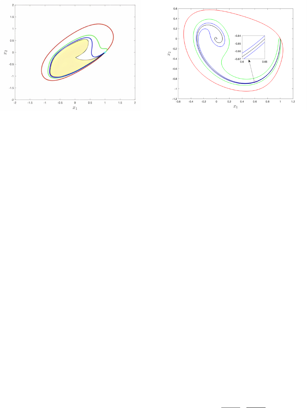
Fig. 1: Simulated response of system (3) with parameters
(14). The light yellow region represents the set of reachable
states from x
0
, the cyan point. The red, green and blue
regions represent the approximation of the reachable set
using 4
th
, 8
th
and 12
th
order non-homogeneous polynomials
computed by solving (13) respectively.
Remark 2: The reachable sets X
i
produced by solving
(13) are invariant which means that for any trajectory x
which starts at x
0
∈ X
i
under the dynamics (3), x(t) ∈ X
i
for all t > 0.
From figure 1, the set of reachable states from a given
initial condition is not symmetric around the origin, so
finding the outer approximation for this set by means of
non-homogeneous polynomials gives more accurate approx-
imations than homogeneous polynomials that are symmetric
around the origin. That makes the approximations presented
here far better than those introduced in [6]. Motivated by the
excellent performance obtained when considering example 1,
we then examine the kind of reachable set approximation that
may be obtained for a LTI system running from a given initial
condition. That can be illustrated by the following example.
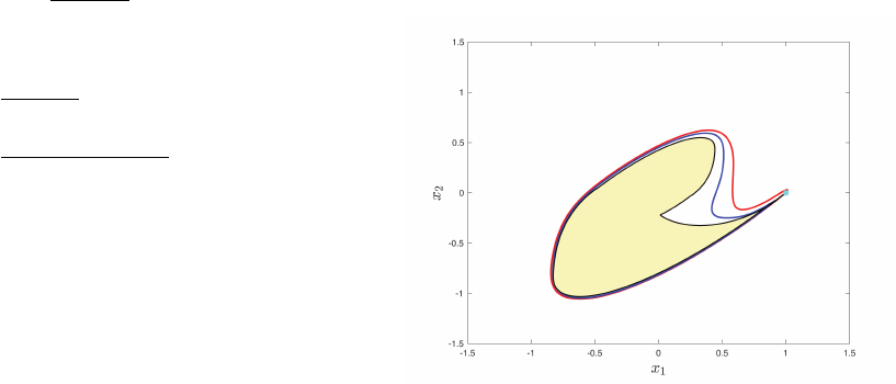
Example 2: Consider the linear time invariant (LTI) sys-
tem
˙x =
0 1
−2 −1
x, x
0
=
1
0
. (15)
The semi-definite program (13) is solved to bound the
system trajectory by a non-homogeneous polynomial for
i = 2, 3, and 4 that generates 4-th, 6-th and 8-th non-
homogenuous order polynomials respectively. Figure 2 illus-
trates that increasing the order of the non-homogeneous poly-
nomial produces increasingly accurate invariant polynomial
outer approximations for that system’s specific trajectory.
Fig. 2: The black line represents the simulated response of
system (15) . The red, green and blue regions represent
the approximation of the reachable set using 4
th
, 6
th
and
8
th
non-homgenuous polynomials computed by solving (13)
respectively.
In the next section, the introduced hierarchy of non-
homogeneous Lyapunov function is used to compute less
conservative bounds for the impulse response of both LTI
systems and LTV systems.
V. ANALYSIS OF IMPULSE RESPONSE VIA
NON-HOMOGENEOUS LYAPUNOV FUNCTIONS
In this section, we consider the single-input, single-output
LTV system
˙x = A(t)x + bu, y = cx, (16)
where u and y are the system’s input and output respectively.
The impulse response h(t) of the system (16) is given by the
output of the system
˙z(t) = A(t)z(t), h(t) = cz(t), (17)
with initial condition z(0) = b. The objective is reducing
the conservatism of the bounds on the peak of the impulse
response for system (16) generated using quadratic Lyapunov
functions. This conservatism has been quantified in [1, page
98] or [18]. The augmented system (17) allows us to take
advantage of the hierarchy (10). Then, system (17) can be
lifted to level i ≥ 2 as
˙
˜
ξ
i
=
˜
A
i
(t)
˜
ξ
i
, h
i
(t) =
˜
c
i
˜
ξ
i
(18)
where
˜
ξ
i
(0) =
˜
b
i
=
b
T
(⊗
2
b)
T
. . . (⊗
i
b)
T
T
. and
˜
c
i
=
c ⊗
2
c . . . ⊗
i
c
. In this case, h
i
(t) = h(t) + h(t)
2
+ · · · +
h(t)
i
.
Theorem 2: The impulse response of (16) satisfies |h(t)|≤
¯
h
i
, where
¯
h
i
is the unique real positive root of the polynomial
p
i
+ p
i−1
+ · · · + p −
¯
h
i
where
¯
h
i
=
q
˜
c
i
P
i
˜
c
T
i
q
˜
b
T
i
P
i
˜
b
i
(19)
for any P
i
satisfies (11).

Proof: Since P
i
satisfies (11) for the system (18), the
set X
i
= {
˜
ξ
i
|
˜
ξ
T
i
P
i
˜
ξ
i
≤
˜
b
T
i
P
i
˜
b
i
} is invariant. Hence,
the maximum output
¯
h
i
is the solution of the optimization
problem
¯
h
i
= max
˜
ξ
i
˜
c
i
˜
ξ
i
,
s.t.
˜
ξ
T
i
P
i
˜
ξ
i
≤
˜
b
T
i
P
i
˜
b
i
.
(20)
By applying KKT conditions, (20) can be solved by
¯
h
i
=
p
˜
c
i
P
i
˜
c
T
i
q
˜
b
T
i
P
i
˜
b
i
. which means that |h(t) + h(t)
2
+ · · · +
h(t)
i
|≤
¯
h
i
, then, |h(t)|+|h(t)|
2
+ · · · + |h(t)|
i
≤
¯
h
i
. Hence,
|h(t)|≤
¯
h
i
where
¯
h
i
is root of the polynomial p
i
+ p
i−1
+
· · · + p −
¯
h
i
. This polynomial has only one real positive
root for i ≥ 1 because
¯
h
i
> 0 and p
i
+ p
i−1
+ · · · + p is
an increasing function of p for p ≥ 0. Therefore, only one
value of p ∈ R
+
satisfies p
i
+ p
i−1
+ · · · + p −
¯
h
i
= 0 which
completes the proof.
The results of theorem 2 can be improved by optimizing
(19) over all possible P
i
. This is done by solving the convex
optimization problem
P
i
= arg min
Q
˜
c
i
Q
−1
˜
c
T
s.t.
˜
b
T
i
Q
˜
b
i
≤ 1
(
˜
A
i
j
)
T
Q + Q
˜
A
i
j
⪯ 0.
(21)
In the following example, we apply theorem 2 for a sys-
tem with stiff dynamics where the bounds of the impulse
response obtained using quadratic Lyapunov functions are
conservative [18].
Example 3: Consider the following system with stiff dy-
namics, that is presented in [12],
˙x =
−1 0
0 −100
x +
1
1
u, y =
1 −2
x. (22)
The optimization problem (21) is solved for i = 1, 3, and 5,
then the resulted P
i
is used to get an upper bound for the
peak of the impulse response by utilizing theorem 2. Figure 3
shows that using higher order non-homogeneous polynomial
Lyapunov function significantly reduces the conservatism in
the impulse response bound of system (22) compared to
quadratic Lyapunov function.
Fig. 3: In the left figure , the black line represents the
phase portrait of the impulse response of system (22). The
red, green and blue level sets represent the invariant sets
produced by solving (21) for i = 1, 3 and 5 respectively. In
the right figure, the black line is the impulse response of the
system (22). The red, green and blue lines present the bounds
obtained by theorem 2 at i = 1, 3, and 5 respectively.
In the next example, we show the effectiveness of using
non-homogeneous Lyapunov functions to provide upper and
lower bounds for the peak of the impulse response for
uncertain systems. The upper bound is obtained by utiliz-
ing theorem 2 then Lyapunov-like function resulting from
solving (21) is used to generate a worst case trajectory [19].
Such a trajectory can be defined by using a Lyapunov-like
function to guide the choice of A(t) at every t ≥ 0.
Definition 1: For a given continuously differentiable func-
tion V (x), a worst case trajectory is defined as a trajectory
ϕ(t; x
0
) that solves (3) with initial condition x
0
and A(t)
given by
A
w
(t; V ) = arg max
A(t)∈conv(M)
˙
V (ϕ(t; x
0
)). (23)
Intuitively, a choice of A(t) that minimizes the decay rate
of the Lyapunov function is ”worst case”.
Example 4: Consider the uncertain system (16) such that
A(t) = A + λ(t)∆ where λ ∈ [−1, 1],
A =
0 1
−0.6 −0.5
, ∆ =
0 0
0.1 −0.1
(24)
b =
0 1
T
and c =
1 0
. In this case, M = {A +
∆, A − ∆}. The optimization problem (21) is solved for
different values of i. Then, theorem 2 is employed to get the
upper bound for the impulse response peak. The resulting
bounds for i = 1, 5, 10 and 12 are 0.9929, 0.9094, 0.8973
and 0.8958 respectively.
The Lyapunov-like function V (x) =
˜
ξ
i
P
i
˜
ξ
i
is used to
generate a worst case trajectory by solving (23). Hence
A
w
(t) = A + λ
max
(t)∆ such that λ
max
(t) solves
arg max
λ
˜
ξ
i
(t)
T
h
P
i
(
˜
A
i
+ λ
˜
D
i
) + (
˜
A
i
+ λ
˜
D
i
)
T
P
i
i
˜
ξ
i
(t)
where
˜
D
i
= diag(D
1
, D
2
, . . . , D
i
) such that D
1
= ∆ and
D
k
= I
n
⊗ D
k−1
+ ∆ ⊗ I
n
k−1
for k = 2, . . . , i. Therefore,
λ
max
(t) = sign(
˜
ξ
i
(t)
T
P
i
˜
D
i
+
˜
D
T
i
P
i
˜
ξ
i
(t)). The lower
bound for the impulse response peak is max
t
y
w
(t) where
y
w
is the output of the generated worst case trajectory. For
i = 12, the lower bound is 0.8901 where the upper bound is
0.8958 which shows the effectiveness of non-homogeneous
Lyapunov function in introducing tight bounds for the peak
of the impulse response of LTV systems.
VI. EXTENSION TO INVARIANT SETS COMPUTATION
In this section, we extend our results to compute polyno-
mial invariant sets that are not Lyapunov functions. We can
use the following example to show that not every invariant
set is a Lyapunov function level set and can be characterized
via S procedure. Consider the simple system
˙x =
−1 0
0 −1
x (25)
We define the set
S(x) = {x ∈ R
2
: (x−x
0
)
T
(x−x
0
) = 3}, with x
0
= [1 1]
T
.
First, it is clear that V (x) = (x − x
0
)
T
(x − x
0
) is not a
Lyapunov function for (25) since
˙
V (x) = −2(x − x
0
)
T
x
= x
T
0
x
0
when x = x
0
= 1.
We now show that the invariance of V can be established by
means of classical S procedure. we need to show that
−(x − x
0
)
T
x ≤ 0 whenever (x − x
0
)
T
(x − x
0
) = 3.
For that purpose, it is sufficient to show that there exists a
number λ such that
−(x − x
0
)
T
x + λ
(x − x
0
)
T
(x − x
0
) − 3
≤ 0 ∀x
For x = x
0
, −(x − x
0
)
T
x + λ
(x − x
0
)
T
(x − x
0
) − 3
=
−3λ, thus λ must be greater than 0. When (x−x
0
)
T
(x−x
0
)
is large, then −(x − x
0
)
T
x + λ
(x − x
0
)
T
(x − x
0
) − 3
=
(λ−1)(x−x
0
)
T
(x−x
0
)(1+o(1)), Thus, λ must be smaller
than 1. Introduce v = x − x
0
. Then,
− (x − x
0
)
T
x + λ
(x − x
0
)
T
(x − x
0
) − 3
= − v
T
v − v
T
x
0
+ λv
T
v − 3λ
=(λ − 1)v
T
v − v
T
x
0
− 3λ
The condition of maximality of this expression is
v =
1
2(λ − 1)
x
0
and thus the maximum of (λ − 1)v
T
v − v
T
x
0
− 3λ is
−1
4(λ − 1)
x
T
0
x
0
− 3λ
=
−1/2 − 3λ(λ − 1)
λ − 1
Choosing λ = 0.5 makes this maximum negative, thus
demonstrating that S is invariant. Therefore, the quadratic
Lyapunov function for the system hierarchy discussed in
Section IV can be effectively generalized to polynomial
invariant sets that are not necessarily Lyapunov functions
by introducing the symmetric matrix
¯
P
i
=
P
i
q
i
q
T
i
r
i
,
for every i ≥ 1 in the hierarchy ,where P
i
∈ R
˜n
i
טn
i
, q
i
∈
R
˜n
i
, and r
i
∈ R. We then consider the quadratic-affine
function
¯
V (
˜
ξ
i
) =
˜
ξ
i
1
T
¯
P
i
˜
ξ
i
1
and we pose the question of the invariance of the set
¯
E
i
=
n
˜
ξ
i
∈ R
˜n
i
such that
¯
V (
˜
ξ
i
) ≤ 0
o
under the action of the system
˜
H
i
in the hierarchy (10).
Then, the invariance question can be posed as asking whether
˙
¯
V ≤ 0 whenever
¯
V (
˜
ξ
i
) = 0 which can be written as
˜
ξ
i
1
T
¯
P
i
˜
A
i
j
˜
ξ
i
0
+
˜
A
i
j
˜
ξ
i
0
T
¯
P
i
˜
ξ
i
1
≤ 0
for all j = 1, . . . , N whenever
˜
ξ
i
1
T
¯
P
i
˜
ξ
i
1
= 0.
By applying S procedure, that holds if and only if there
exists a real number λ such that
˜
ξ
i
1
T
¯
P
i
˜
A
i
j
˜
ξ
i
0
+
˜
A
i
j
˜
ξ
i
0
T
¯
P
i
˜
ξ
i
1
+ λ
˜
ξ
i
1
T
¯
P
i
˜
ξ
i
1
≤ 0
for j = 1, . . . , N and for all
˜
ξ
i
∈ R
˜n
i
, that is, the matrix
¯
P
i
˜
A
i
j
+ (
˜
A
i
j
)
T
¯
P
i
+ λ
¯
P
i
(
˜
A
i
j
)
T
q + λq
q
T
˜
A
i
j
+ λq
T
λr
(26)
is negative semi-definite for all j = 1, . . . , N . for a fixed
value of λ, looking for
¯
P
i
such that (26) is negative semi-
definite is convex in
¯
P
i
. In particular, setting λ = 0 brings
back the search for a polynomial Lyapunov function. Other
values of λ then offer other options for finding polynomial
invariant sets. The authors in [20] developed a method
to construct a Lyapunov function of degree 1 from the
invariant set. This homogeneous Lyapunov function is called
Algebraic Lyapunov function. For the system presented in
example 1, the convex feasibility problem (26) is solved for
i = 5 and 7 and for λ = −0.05 to find the invariant set
passing through the initial condition x
0
= [1 0]
T
. The results
are shown in figure 4.
Fig. 4: Simulated response for system presented in example
1. The light yellow region represents the set of reachable
states from the initial condition x
0
. The red and blue regions
represents the non-homogeneous polynomial invariant sets
resulted from solving (26) for i = 5 and 7 respectively and
for λ = −0.05.
VII. RELATION TO POLYNOMIAL LYAPUNOV FUNCTIONS
OBTAINED VIA ”SUM-OF-SQUARES” SEMIDEFINITE
RELAXATION METHODS
The authors believe the foregoing quadratic Lyapunov
functions are in direct correspondence with the polynomial
Lyapunov functions for System (3) that may be computed
by means of ”Sum-of-Square” relaxations, and we formulate
the following conjecture:

Conjecture: There exists a positive definite matrix P
i
∈
R
˜n
i
טn
i
that satisfies
P
i
˜
A
i
j
+ (
˜
A
i
j
)
T
P
i
⪯ 0 for all j = 1, . . . , N
if and only if there exists a polynomial G(x) of degree 2i
with G(0) = 0 and G(x) > 0, x ̸= 0, satisfying
∂G
∂x
.A
j
x < 0 for all j = 1, . . . , N
proving that conjecture is left for future work.
VIII. CONCLUSION AND FUTURE WORK
This work presents a procedure to compute non-
homogeneous polynomial Lyapunov functions and invariant
sets for LTV systems. This procedure is based on build-
ing a hierarchy of LTV systems such that the quadratic
Lyapunov function for any system in the hierarchy is a
non-homogeneous polynomial Lyapunov function for the
base level system. These non-homogeneous polynomials are
shown to be effective in LTV systems performance analysis
by computing outer approximation for the reachable sets,
bounds for the impulse response and invariant sets that are
not Lyapunov level sets. In future work, the theoretical re-
lation between the generated non-homogeneous polynomials
and other polynomials computed by means of Sum-of-Square
relaxations will be considered.
REFERENCES
[1] S. Boyd, L. El Ghaoui, E. Feron, and V. Balakrishnan, Linear matrix
inequalities in system and control theory. SIAM, 1994.
[2] A. A. Ahmadi and P. A. Parrilo, “Sum of squares certificates for stabil-
ity of planar, homogeneous, and switched systems,” IEEE Transactions
on Automatic Control, vol. 62, no. 10, pp. 5269–5274, 2017.
[3] P. Mason, U. Boscain, and Y. Chitour, “Common polynomial Lya-
punov functions for linear switched systems,” SIAM journal on control
and optimization, vol. 45, no. 1, pp. 226–245, 2006.
[4] D. Liberzon, Switching in systems and control, vol. 190. Springer,
2003.
[5] A. Zelentsovsky, “Nonquadratic Lyapunov functions for robust sta-
bility analysis of linear uncertain systems,” IEEE Transactions on
Automatic control, vol. 39, no. 1, pp. 135–138, 1994.
[6] M. Abate, C. Klett, S. Coogan, and E. Feron, “Lyapunov differ-
ential equation hierarchy and polynomial Lyapunov functions for
switched linear systems,” in 2020 American Control Conference
(ACC), pp. 5322–5327, IEEE, 2020.
[7] P. A. Parrilo, “Semidefinite programming relaxations for semialgebraic
problems,” Mathematical programming, vol. 96, pp. 293–320, 2003.
[8] Z. Jarvis-Wloszek, R. Feeley, W. Tan, K. Sun, and A. Packard,
“Control applications of sum of squares programming,” Positive poly-
nomials in control, pp. 3–22, 2005.
[9] P. A. Parrilo, Structured semidefinite programs and semialgebraic
geometry methods in robustness and optimization. California Institute
of Technology, 2000.
[10] J. Abedor, K. Nagpal, and K. Poolla, “A linear matrix inequality
approach to peak-to-peak gain minimization,” International Journal of
Robust and Nonlinear Control, vol. 6, no. 9-10, pp. 899–927, 1996.
[11] F. Blanchini, “Nonquadratic Lyapunov functions for robust control,”
Automatica, vol. 31, no. 3, pp. 451–461, 1995.
[12] M. Abate, C. Klett, S. Coogan, and E. Feron, “Pointwise-in-time
analysis and non-quadratic Lyapunov functions for linear time-varying
systems,” in 2021 American Control Conference (ACC), pp. 3550–
3555, IEEE, 2021.
[13] H. Abdelraouf, G.-Y. Immanuel, and E. Feron, “Computing bounds
on l
∞
-induced norm for linear time-invariant systems using homoge-
neous Lyapunov functions,” arXiv preprint arXiv:2203.00716, 2022.
[14] H. Lin and P. J. Antsaklis, “Stability and stabilizability of switched
linear systems: a survey of recent results,” IEEE Transactions on
Automatic control, vol. 54, no. 2, pp. 308–322, 2009.
[15] G. Chesi, A. Garulli, A. Tesi, and A. Vicino, Homogeneous polynomial
forms for robustness analysis of uncertain systems, vol. 390. Springer
Science & Business Media, 2009.
[16] L. Vandenberghe and S. Boyd, “A polynomial-time algorithm for
determining quadratic Lyapunov functions for nonlinear systems,” in
Eur. Conf. Circuit Th. and Design, pp. 1065–1068, 1993.
[17] M. Grant and S. Boyd, “Cvx: Matlab software for disciplined convex
programming, version 2.1,” 2014.
[18] E. Feron, “Linear matrix inequalities for the problem of absolute
stability of control systems,” Ph.D. Thesis, Stanford University, 1994.
[19] C. Klett, M. Abate, S. Coogan, and E. Feron, “A numerical method
to compute stability margins of switching linear systems,” in 2021
American Control Conference (ACC), pp. 864–869, IEEE, 2021.
[20] H. Abdelraouf, E. Feron, and J. Shamma, “Algebraic Lyapunov
functions for homogeneous dynamic systems,” arXiv preprint
arXiv:2303.02185, 2023.
APPENDIX
A. Dimensionality reduction
Using Kronecker product produces redundant states that
significantly increase the dimension of the lifted system. For
example, if x ∈ R
2
, then ξ
2
∈ R
4
such that ξ
2
= x ⊗ x =
x
2
1
x
1
x
2
x
1
x
2
x
2
2
T
. To get rid of the redundant states,
a simple procedure introduced in [6]. This procedure is based
on introducing a new variable η
2
∈ R
3
such that ξ
2
= W
2
η
2
where
W
2
=
1 0 0
0 1 0
0 1 0
0 0 1
.
For second order systems, i.e. n = 2, this method can be
generalized for k ≥ 2 as ξ
k
= W
k
η
k
such that
W
k
=
W
k−1
0
2
k−1
0
2
k−1
W
k−1
and W
1
= I
2
. So, the dimension of the system H
k
in the
hierarchy (9) is reduced from n
k
to k + 1. Without loss
of generality, if M = {A}, then every system
˙
ξ
k
= A
k
ξ
k
in the hierarchy (9) can be written as ˙η
k
= W
+
k
A
k
W
k
η
k
where W
+
k
is the pseudo-inverse of W
k
for k ≥ 1. We can
then use the reduced dimension state vector η
k
to rebuild
the new hierarchy (10). Hence, ˜η
i
=
η
T
1
, η
T
2
, . . . , η
T
i
T
which reduces the dimension of the system
˜
H
i
in the
hierarchy (10) from 2(2
i
− 1) to i(i + 3)/2. Thus, the
reduced dimension system
˜
H
i
will be ˜η
i
=
˜
W
+
i
˜
A
i
˜
W
i
˜η
where
˜
W
i
= diag(W
1
, W
2
, . . . , W
i
).
