Introduction to LTV Systems Computation of the State Transition Matrix Discretization of Continuous Time Systems
Module 04
Linear Time-Varying Systems
Ahmad F. Taha
EE 5143: Linear Systems and Control
Email: [email protected]
Webpage: http://engineering.utsa.edu/
˜
taha
September 26, 2017
©Ahmad F. Taha Module 04 — Linear Time-Varying Systems 1 / 26
Introduction to LTV Systems Computation of the State Transition Matrix Discretization of Continuous Time Systems
Introduction to State Transition Matrix (STM)
For the linear autonomous system
˙x(t) = Ax(t), x(t
0
) = x
0
, t ≥ 0
the state solution is
x(t) = e
A(t−t
0
)
x
0
Define the state transition matrix (STM):
φ(t, t
0
) = e
A(t−t
0
)
– STM (φ(t, t
0
)) propagates an initial state along the LTI solution t
time forward. Note that:
φ(t
1
+ t
2
, t
0
) = φ(t
1
, t
0
)φ(t
2
, t
0
) = φ(t
2
, t
0
)φ(t
1
, t
0
), ∀t
1
, t
2
≥ 0
In general, for an linear time varying system,
˙x(t) = A(t)x(t) + B(t)u(t), x(t
0
) = x
0
,
the state solution is given in terms of the STM:
x(t) = Φ(t, t
0
)x(t
0
) +
Z
t
t
0
Φ(t, τ)B(τ)u(τ)dτ
©Ahmad F. Taha Module 04 — Linear Time-Varying Systems 2 / 26
Introduction to LTV Systems Computation of the State Transition Matrix Discretization of Continuous Time Systems
Properties of the STM
For the linear autonomous system
˙x(t) = Ax(t), x(t
0
) = x
0
, t ≥ 0
the STM is:
φ(t, t
0
) = e
A(t−t
0
)
1
φ(t
0
, t
0
) = φ(t, t) = I
2
φ
−1
(t
1
, t
2
) = φ(t
2
, t
1
)
3
φ(t
1
, t
2
) = φ(t
1
, t
0
)φ(t
0
, t
2
)
4
d
dt
(φ(t, t
0
)) = Aφ(t, t
0
)
Proofs:
©Ahmad F. Taha Module 04 — Linear Time-Varying Systems 3 / 26
Introduction to LTV Systems Computation of the State Transition Matrix Discretization of Continuous Time Systems
Solution Space and System Modes
Solution space X of the LTI system ˙x (t) = Ax (t) is the set of all
its solutions:
X := {x (t), t ≥ 0 | ˙x = Ax }
X is a vector space
Dimension of X is n
System modes: A mode of the LTI system ˙x = Ax is its solution
from an eigenvector of A:
x(t) = e
At
v
i
= e
λ
i
t
v
i
This is one property of the matrix exponential (see Module 3)
The n (possibly repeated) modes form a basis of the solution space
X
©Ahmad F. Taha Module 04 — Linear Time-Varying Systems 4 / 26
Introduction to LTV Systems Computation of the State Transition Matrix Discretization of Continuous Time Systems
Decomposition of State Solution
Any state solution for an autonomous system can be written as a
linear combination of system modes, assuming that A is
diagonalizable
This means that the solution space X can be formed by these linear
combinations
A = TDT
−1
is assumed to be diagonalizable
Assume that we start from x
0
= TT
−1
x
0
= x
0
This means that we start from a linear combinations of
v
i
, i = 1, . . . , n since
x
0
= TT
−1
x
0
=
n
X
i=1
(x
>
0
w
i
)v
i
=
n
X
i=1
α
i
v
i
where w
i
’s are the rows of the T
−1
matrix (or the left evectors)
Given that construction, we can see that the solution x (t) is a LC of
the modes e
λ
i
t
v
i
©Ahmad F. Taha Module 04 — Linear Time-Varying Systems 5 / 26
Introduction to LTV Systems Computation of the State Transition Matrix Discretization of Continuous Time Systems
Changing Coordinates
Changing of coordinates of an LTI system: basically means we’re
scaling the coordinates in a different way
Assume that T ∈ R
n×n
is a nonsingular transformation matrix
Define ˜x = T
−1
x. Recall that ˙x = Ax + Bu, then:
˙
˜x = (T
−1
AT )˜x + T
−1
Bu =
˜
A˜x +
˜
Bu
with initial conditions ˜x (0) = T
−1
x(0)
Remember the diagonal canonical form? We can get to it if the
transformation T is the matrix containing the eigenvectors of A
What if the matrix is not diagonlizable? Well, we can still write
A = TJT
−1
, which means that
˜
A = J is the new state-space matrix
via the eigenvector transformation
In fact, you can show that if A = TJT
−1
with j Jordan blocks (i.e.,
J = diag(J
1
, J
2
, . . . , J
j
), then after the transformation ˜x = T
−1
x,
the LTI system becomes decoupled:
˙
˜x
1
= J
1
˜x
1
,
˙
˜x
2
= J
2
˜x
2
, . . . ,
˙
˜x
j
= J
j
˜x
j
.
©Ahmad F. Taha Module 04 — Linear Time-Varying Systems 6 / 26
Introduction to LTV Systems Computation of the State Transition Matrix Discretization of Continuous Time Systems
STM of LTV Systems
In the previous module, we learned how to compute the state and
output solution
We assumed that the system is time invariant, i.e.,
˙x(t) = Ax(t) + Bu(t)
What if the system is time varying:
˙x(t) = A(t)x(t) + B(t)u(t), y(t) = C(t)x(t) + D(t)u(t) (∗)
How can we compute x(t) and y(t)?
That relies on finding the STM of the LTV system (∗)
To do so, we have to find the exponential of a time-varying matrix
©Ahmad F. Taha Module 04 — Linear Time-Varying Systems 7 / 26

Introduction to LTV Systems Computation of the State Transition Matrix Discretization of Continuous Time Systems
STM of LTV Systems — 2
Theorem — STM of ˙x(t) = A(t)x(t)
The STM of ˙x(t) = A(t)x(t) + B(t)u(t) is given by
φ(t, t
0
) = exp
Z
t
t
0
A(q)dq
if the following conditions are satisfied:
1
A(t) has piecewise continuous entries for all t, t
0
a
2
A(t) commutes with its integral M(t, t
0
) =
R
t
t
0
A(q)dq, i.e.,
A(t)M(t, t
0
) = M(t, t
0
)A(t)
a
A function is piecewise continuous if: (a) it is defined throughout that interval, (b)
its functions are continuous on that interval, and (c) there is no discontinuity at the
endpoints of the defined interval.
This theorem is very important, but can be very difficult to assess
Consider a large system with TV A(t). Then, numerical integration
needs to be performed the check the conditions
©Ahmad F. Taha Module 04 — Linear Time-Varying Systems 8 / 26

Introduction to LTV Systems Computation of the State Transition Matrix Discretization of Continuous Time Systems
STM of LTV Systems — 3
Given this analytical challenge, a natural question arises
What are easily testable conditions that are sufficient for A(t) to
commute with M(t, t
0
)?
The following theorem investigates this question
Theorem — STM Testing Conditions
A(t) and M(t, t
0
) commute if any of the following conditions hold:
1
A(t) = A is a constant matrix
2
A(t) = β(t)A where β(·) : R → R is a scalar function and A is a
constant matrix
3
A(t) =
P
m
i=1
β
i
(t)A
i
where β
i
(·) : R → R are all scalar functions
and A
i
’s are all constant matrices that commute with each other,
i.e., A
i
A
j
= A
j
A
i
, ∀i, j ∈ {1, 2, . . . , m}
4
There exists a factorization A(t) = TD(t)T
−1
where
D(t) = diag(λ
1
(t), . . . , λ
n
(t))
©Ahmad F. Taha Module 04 — Linear Time-Varying Systems 9 / 26
Introduction to LTV Systems Computation of the State Transition Matrix Discretization of Continuous Time Systems
Example 1
A(t) = ˙α(t)
a −a
a −a
What is the state transition matrix?
Solution: notice that A(t) fits with the second characterization,
hence A(t) and M(t, t
0
) commute (assume that α(t) is continuous
differentiable function)
Note that A is nilpotent of order 2
Solution:
φ(t, t
0
) = exp
Z
t
t
0
A(q)dq
= I +
a −a
a −a
(α(t) − α(t
0
))
©Ahmad F. Taha Module 04 — Linear Time-Varying Systems 10 / 26
Introduction to LTV Systems Computation of the State Transition Matrix Discretization of Continuous Time Systems
Example 2
A(t) =
˙a(t)
˙
b(t)
˙
b(t) ˙a(t)
, find the STM
Note that A(t) = ˙a(t)I +
˙
b(t)
0 1
1 0
We can apply the third case to obtain:
φ(t, t
0
) = exp
Z
t
t
0
A(q)dq
= e
a(t)−a(t
0
)
exp
0 b(t) − b(t
0
)
b(t) − b(t
0
) 0
Recall that if
A
2
=
0 b
b 0
⇒ e
A
2
t
=
cosh(bt) sinh(bt)
sinh(bt) cosh(bt)
Hence,
φ(t, t
0
) = e
a(t)−a(t
0
)
cosh(b(t) − b(t
0
)) sinh(b(t) − b(t
0
))
sinh(b(t) − b(t
0
)) cosh(b(t) − b(t
0
))
©Ahmad F. Taha Module 04 — Linear Time-Varying Systems 11 / 26
Introduction to LTV Systems Computation of the State Transition Matrix Discretization of Continuous Time Systems
Overall Solution
So, given that we have the state transition matrix, how can we find
the overall solution of the LTV system?
The answer is simple:
x(t) = φ(t, t
0
)x(t
0
) +
Z
t
t
0
φ(t, τ)B(τ)u(τ)dτ
©Ahmad F. Taha Module 04 — Linear Time-Varying Systems 12 / 26
Introduction to LTV Systems Computation of the State Transition Matrix Discretization of Continuous Time Systems
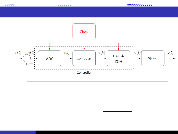
Intro to Discretization
We want to discretize and transform this dynamical system
˙x(t) = Ax(t) + Bu(t)
y(t) = Cx (t) + Du(t)
to
x(k + 1) =
˜
Ax(k) +
˜
Bu(k)
y(k) =
˜
Cx(k) +
˜
Du(k)
Why do we need that?
Because if you want to use a computer to compute numerical
solutions to the ODE, you’ll have to give the computer a language it
understands
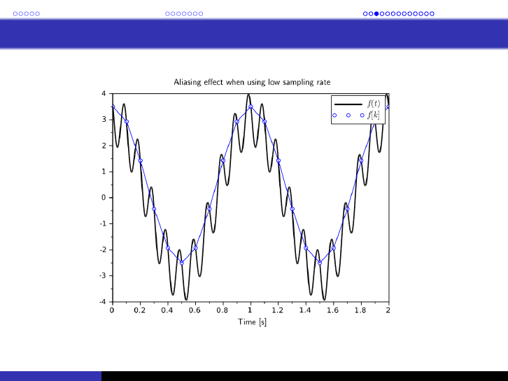
Also, many dynamical systems are naturally discrete, not continuous,
i.e., sampling doesn’t happen continuously
©Ahmad F. Taha Module 04 — Linear Time-Varying Systems 14 / 26
Introduction to LTV Systems Computation of the State Transition Matrix Discretization of Continuous Time Systems
What Computers Understand
What is zero order hold? It’s basically the model of the signal
reconstruction of the digital to analog converter (DAC):
u
ZOH
(t) =
∞
X
k=−∞
u(k) · rect
t − T /2 − kT
T
©Ahmad F. Taha Module 04 — Linear Time-Varying Systems 15 / 26
Introduction to LTV Systems Computation of the State Transition Matrix Discretization of Continuous Time Systems
Discretization — 1
1
Use the derivative rule:
˙x(t) = lim
T →0
x(t + T ) − x(t)
T
2
You can use this approximation:
x(t + T ) − x(t)
T
= Ax(t)+Bu(t) ⇒ x(t+T ) = x (t)+ATx(t)+BTu(t)
3
Hence,
x(t + T ) = (I + AT )x(t) + BTu(t)
4
Now, if we compute x(t) and y(t) only at t = kT for k = 0, 1, . . . ,
then the dynamical system equation for the discretized, approximate
system is:
x((k + 1)T ) = (I + AT )
| {z }
˜
A
x(kT ) + BT
|{z}
˜
B
u(kt)
y(kT ) =
˜
Cx(kT ) +
˜
Du(kT )
©Ahmad F. Taha Module 04 — Linear Time-Varying Systems 17 / 26
Introduction to LTV Systems Computation of the State Transition Matrix Discretization of Continuous Time Systems
Discretization — 2
The aforementioned discretization is a valid discretization for a
continuous time system
This method is based on forward Euler differentiation method
Easily computed by the computer, i.e., no need for matrix
exponentials—just simple computations
While this discretization is the easiest, it’s the least accurate
Solution: a different discretization method
©Ahmad F. Taha Module 04 — Linear Time-Varying Systems 18 / 26
Introduction to LTV Systems Computation of the State Transition Matrix Discretization of Continuous Time Systems
Another Discretization Method — 1
Recall that if the input u(t) is generated by a computer then
followed by DAC, then u(t) will be piecewise constant:
u(t) = u(kT ) =: u(k) for kT ≤ t ≤ (k+1)T , k = 0, 1, . . . , k
f
Note that this input only changes values at discrete time instants
Recall the solution to the state-equation:
x(t) = e
At
x(0) +
Z
t
0
e
A(t−τ )
Bu(τ)dτ
Setting t = KT in the previous equation, then we can write:
x(k) := x(kT ) = e
AkT
x(0) +
Z
kT
0
e
A(kT −τ )
Bu(τ)dτ
x(k+1) := x((k+1)T ) = e
A(k+1)T
x(0)+
Z
(k+1)T
0
e
A((k+1)T −τ )
Bu(τ)dτ
©Ahmad F. Taha Module 04 — Linear Time-Varying Systems 19 / 26
Introduction to LTV Systems Computation of the State Transition Matrix Discretization of Continuous Time Systems
Another Discretization Method — 2
x(k + 1) := x ((k + 1)T ) = e
A(k+1)T
x(0) +
Z
(k+1)T
0
e
A((k+1)T −τ )
Bu(τ)dτ
Note that the above equation can be written as:
x(k + 1) = e
AT
e
AkT
x(0) +
Z
kT
0
e
A(kT −τ )
Bu(τ)dτ
!
+
Z
(k+1)T
kT
e
A(kT +T −τ )
Bu(τ)dτ
Recall that we’re assuming that:
u(t) = u(kT ) =: u(k) for kT ≤ t ≤ (k+1)T , k = 0, 1, . . . , k
f
i.e., the input is constant between two sampling instances
Look at x (k) and let α = kT + T − τ , then:
x(k + 1) = e
AT
x(k) +
Z
T
0
e
Aα
dα
!
Bu(k)
©Ahmad F. Taha Module 04 — Linear Time-Varying Systems 20 / 26
Introduction to LTV Systems Computation of the State Transition Matrix Discretization of Continuous Time Systems
Another Discretization Method — 3
x(k + 1) = e
AT
x(k) +
Z
T
0
e
Aα
dα
!
Bu(k)
Hence, the discretized system with sampling time-period T can be
written as:
x(k + 1) =
˜
Ax(k) +
˜
Bu(k)
y(k) =
˜
Cx(k) +
˜
Du(k)
where
˜
A = e
AT
,
˜
B =
Z
T
0
e
Aα
dα
!
B,
˜
C = C ,
˜
D = D
Note that there is no approximation in this solution
We only assumed that u(k) is piecewise constant between the two
sampling instances
It’s easy to compute the new discretized SS matrices (besides
˜
B)
©Ahmad F. Taha Module 04 — Linear Time-Varying Systems 21 / 26
Introduction to LTV Systems Computation of the State Transition Matrix Discretization of Continuous Time Systems
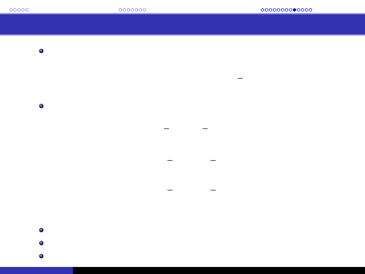
Another Discretization Method — 4
To compute
˜
B, you can simply evaluate the formula:
˜
B =
Z
T
0
e
Aα
dα
!
B =
Z
T
0
I + Aα +
1
2
A
2
α
2
+ . . . dα
!
B
Which can be evaluated:
˜
B =
TI +
1
2
T
2
A +
1
3
T
3
A
2
+ . . .
B
= A
−1
TA +
1
2
T
2
A
2
+
1
3
T
3
A
3
+ . . .
B
= A
−1
I + TA +
1
2
T
2
A
2
+
1
3
T
3
A
3
+ . . . − I
B
⇒
˜
B = A
−1
(
˜
A − I)B
This result is only valid for nonsingular A
This formula helps in avoiding infinite series
You can also use MATLAB’s c2d(A,B,...) command
©Ahmad F. Taha Module 04 — Linear Time-Varying Systems 22 / 26
Introduction to LTV Systems Computation of the State Transition Matrix Discretization of Continuous Time Systems
Examples
Discretize the following CT-LTI system:
˙x(t) =
−1 1
0 2
x(t) +
2 0
0 4
u(t)
where the controller’s sampling time is T = 0.1 sec.
We can try the three approaches we learned:
1
Approach 1:
˜
A = I + AT =
0.9 0.1
0 1.2
,
˜
B = BT =
0.2 0
0 0.4
2
Approach 2:
˜
A = e
AT
=
e
−T
1
3
(e
2T
− e
−T
)
0 e
2T
=
0.9048 0.1055
0 1.2214
˜
B =
Z
T
0
e
Aα
dα
!
B = int(expm(A*h),h,0,T)*B =
0.1903 0.0207
0 0.4428
©Ahmad F. Taha Module 04 — Linear Time-Varying Systems 23 / 26
Introduction to LTV Systems Computation of the State Transition Matrix Discretization of Continuous Time Systems
Examples (Cont’d)
Approach 3:
˜
A = e
AT
=
e
−T
1
3
(e
2T
− e
−T
)
0 e
2T
=
0.9048 0.1055
0 1.2214
˜
B = A
−1
(
˜
A − I)B =
0.1903 0.0207
0 0.4428
What do we notice? What are some preliminary conclusions?
©Ahmad F. Taha Module 04 — Linear Time-Varying Systems 24 / 26
Introduction to LTV Systems Computation of the State Transition Matrix Discretization of Continuous Time Systems
Remarks
There’s plenty of other discretization methods in the literature
This question has no specific golden answer
It often depends on the properties of the system
Basically the sampling time period (how often your control is fixed
or changing)
The singularity of the A matrix also plays an important role
©Ahmad F. Taha Module 04 — Linear Time-Varying Systems 25 / 26