
HAL Id: hal-01376819
https://inria.hal.science/hal-01376819
Submitted on 5 Oct 2016
HAL is a multi-disciplinary open access
archive for the deposit and dissemination of sci-
entic research documents, whether they are pub-
lished or not. The documents may come from
teaching and research institutions in France or
abroad, or from public or private research centers.
L’archive ouverte pluridisciplinaire HAL, est
destinée au dépôt et à la diusion de documents
scientiques de niveau recherche, publiés ou non,
émanant des établissements d’enseignement et de
recherche français ou étrangers, des laboratoires
publics ou privés.
Stability of the Kalman lter for continuous time output
error systems
Boyi Ni, Qinghua Zhang
To cite this version:
Boyi Ni, Qinghua Zhang. Stability of the Kalman lter for continuous time output error systems.
Systems and Control Letters, 2016, 94, pp.172 - 180. �10.1016/j.sysconle.2016.06.006�. �hal-01376819�

Stability of the Kalman Filter for Continuous Time Output Error Systems
Boyi Ni
a
, Qinghua Zhang
b
a
SAP Labs China, 1001 Chenhui Rd., Shanghai 201203, China (previously with Inria)
b
Inria, Campus de Beaulieu, 35042 Rennes, France
Abstract
The stability of the Kalman filter is usually ensured by the uniform complete controllability
regarding the process noise and the uniform complete observability of linear time varying systems.
This paper studies the case of continuous time output error systems, in which the process noise is
totally absent. The classical stability analysis assuming the controllability regarding the process
noise is thus not applicable. It is shown in this paper that the uniform complete observability
alone is sufficient to ensure the asymptotic stability of the Kalman filter applied to time varying
output error systems, regardless of the stability of the considered systems themselves. The
exponential or polynomial convergence of the Kalman filter is then further analyzed for particular
cases of stable or unstable output error systems.
Keywords: Kalman filter, Stability, Output error system.
1. Introduction
The well known Kalman filter has been extensively studied and is being applied in many
different fields (Anderson and Moore, 1979; Jazwinski, 1970; Zarchan and Musof, 2005; Kim,
2011; Grewal and Andrews, 2015). The purpose of the present paper is to study the stability
of the Kalman filter in a particular case rarely covered in the literature: the absence of process
noise in the state equation of a linear time varying (LTV) system. Such systems are known as
output error (OE) systems. Though typically process noise and output noise are both considered
in Kalman filter applications, the case with no process noise is of particular interest when state
equations originate from physical laws that are believed accurate enough. Another motivation
of this study is OE system identification (Goodman and Dudley, 1987; Forssell and Ljung, 2000;
Wang et al., 2015). When the prediction error method (Ljung, 1999) is applied to OE system
identification, the stability of the output predictor is a crucial issue. The results presented in
this paper ensure the stability of the predictor based on the Kalman filter.
While the optimal properties of the Kalman filter are frequently recalled, its stability proper-
ties are less often mentioned in the recent literature. The classical stability analysis is based on
both the uniform complete controllability regarding the process noise and the uniform complete
observability of LTV systems (Kalman, 1963; Jazwinski, 1970). In the case of OE systems, there
is no process noise at all in the state equation, hence the controllability regarding the process
Preprint submitted to Systems & Control Letters May 10, 2016
noise cannot be fulfilled, and the classical stability results are not applicable. The present paper
aims at completing this missing case.
The optimal state estimation realized by the Kalman filter can be viewed as a trade-off
between the uncertainties in the state equation and in the output equation. In an OE system,
the state equation is assumed noise-free. This point of view suggests that the state estimation
should solely rely on the state equation, provided that the initial state of the OE system is exactly
known. In practice the Kalman filter remains useful when the initial state is not exactly known
or when the OE system is unstable. Of course, if the state of an unstable system diverges, so does
its state estimate by the Kalman filter. Typically in practice, unstable systems are stabilized
by feedback controllers so that the system state remains bounded. The Kalman filter can be
applied either to the controlled system itself or to the entire closed loop system. In the latter
case, the controller must be linear and completely known, excluding the saturation protection
and any other nonlinearities.
The classical optimality results of the Kalman filter are also valid in the case of OE systems
(Jazwinski, 1970, chapter 7). However, it is necessary to complete the stability analysis, as the
classical results are not applicable in this case.
The main results presented in this paper are as follows. Under the uniform complete observ-
ability condition, it is first shown that the dynamics of the Kalman filter applied to a continuous
time OE LTV system is asymptotically stable, regardless of the stability of the system itself. The
exponential or polynomial convergence of the Kalman filter is further established, depending on
the stability or the instability property of the considered system. The boundedness of the solu-
tion of the Riccati equation, and thus also of the Kalman gain, is also proved under the same
condition. These results complete the classical results (Kalman, 1963; Jazwinski, 1970), which
exclude the case of OE systems.
For linear time invariant (LTI) systems, it is a common practice to design the Kalman filter
by solving an algebraic Riccati equation (in contrast to dynamic differential Riccati equation for
general LTV systems as considered in the present paper). In this case, the controllability and
observability conditions can be replaced by the weaker stabilizability and detectability conditions
(Laub, 1979; Arnold and Laub, 1984).
Some preliminary results about the Riccati equation of time invariant systems have been
presented in the conference paper (Ni and Zhang, 2013), and some further results on the asymp-
totic stability of the Kalman filter have been presented in the conference paper (Ni and Zhang,
2015), without the exponential or polynomial convergence rate analysis and part of the numerical
examples reported in the present paper.
The rest of the paper is organized as follows. Some preliminary elements are introduced in
Section 2. The problem considered in this paper is formulated in Section 3. The asymptotic
stability of the Kalman filter for OE systems is established in Section 4. Exponential and
polynomial convergence rates of the Kalman filter are analyzed in Section 5. Some analytical
and numerical examples are presented in Sections 6 and 7. Finally, concluding remarks are
drawn in Section 8.
2. Definitions and preliminary elements
Let us shortly recall some definitions and basic facts about LTV systems, which are necessary
for the following sections.
Let m and n be any two positive integers. For a vector x ∈ R
n
, kxk denotes its Euclidean
2

norm. For a matrix A ∈ R
m×n
, kAk denotes the matrix norm induced by the Euclidean vector
norm, which is equal to the largest singular value of A and known as the spectral norm when
m = n. Then kAxk ≤ kAkkxk for all A ∈ R
m×n
and all x ∈ R
n
. For two real square symmetric
positive definite matrices A and B, A > B means A − B is positive definite.
Let A(t) ∈ R
m×n
be defined for t ∈ R. It is said (upper) bounded if kA(t)k is bounded.
Consider the homogeneous LTV system
dx(t)
dt
= A(t)x(t) (1)
with x(t) ∈ R
n
and A(t) ∈ R
n×n
, and let Φ(t, t
0
) be the associated state transition matrix such
that, for all t, t
0
∈ R, dΦ(t, t
0
)/dt = A(t)Φ(t, t
0
) and Φ(t, t) = I
n
with I
n
denoting the n × n
identity matrix.
Definition 1. System (1) is Lyapunov stable if there exists a positive constant γ such that, for
all t, t
0
∈ R satisfying t ≥ t
0
, the following inequality holds
kΦ(t, t
0
)k ≤ γ. (2)
This definition concerns the boundedness of the state vector, whereas the following definition
ensures its convergence to zero.
Definition 2. System (1) is asymptotically stable if it is Lyapunov stable and if the following
limiting behavior holds
lim
t→+∞
kx(t)k = 0 (3)
for any initial state x(t
0
) ∈ R
n
.
To characterize the convergence rate of some stable systems, the exponential stability is
defined as follows.
Definition 3. System (1) is exponentially stable if there exist two positive constants α, β such
that the inequality
kΦ(t, t
0
)k ≤ βe
−α(t−t
0
)
(4)
holds for all t, t
0
∈ R satisfying t ≥ t
0
.
The definitions of Lyapunov and exponential stabilities in Definitions 1 and 3 are based on
the norm of the state transition matrix Φ(t, t
0
). They could take another equivalent form, as
suggested by the following lemma. See also (Rugh, 1995).
Lemma 1. Let M ∈ R
n×n
and ξ be some positive scalar value. Then kMk ≤ ξ if and only if
kMvk ≤ ξkvk for all v ∈ R
n
.
See the appendix at the end of this paper for a proof of the lemma.
With M = Φ(t, t
0
), ξ = γ or ξ = βe
−α(t−t
0
)
, Lemma 1 suggests that Definitions 1 and 3
could be based on the norm of x(t) = Φ(t, t
0
)x(t
0
) instead of the norm of Φ(t, t
0
).
3

Definition 4. System (1) is strongly unstable if there exist two positive constants α, β such that
the inequality
kx(t)k ≥ βe
α(t−t
0
)
kx(t
0
)k (5)
holds for all t, t
0
∈ R satisfying t ≥ t
0
and for all x(t
0
) ∈ R
n
.
The following observability definition for LTV systems follows (Kalman, 1963).
Definition 5. The matrix pair [A(t), C(t)] with A(t) ∈ R
n×n
and C(t) ∈ R
m×n
is uniformly
completely observable if there exist positive constants τ , ρ
1
and ρ
2
such that, for all t ∈ R, the
following inequalities hold
1
ρ
1
I
n
≤
Z
t
t−τ
Φ
T
(s, t)C
T
(s)R
−1
(s)C(s)Φ(s, t)ds (6)
≤ ρ
2
I
n
(7)
with some bounded symmetric positive definite matrix R(s) ∈ R
m×m
(typically the covariance
matrix of the output noise in a stochastic state space system).
The fact that observability is preserved by output feedback is stated in the following lemma.
Lemma 2. Let A(t) ∈ R
n×n
, C(t) ∈ R
m×n
, K(t) ∈ R
n×m
be bounded piecewise continuous
matrices. The matrix pair [A(t), C(t)] is uniformly completely observable, if and only if the
matrix pair [A(t) − K(t)C(t), C(t)] is uniformly completely observable.
This lemma can be found in (Anderson et al., 1986, chapter 2). For more rigorous proofs see
(Sastry and Bodson, 1989, chapter 2), (Ioannou and Sun, 1996, chapter 4), and (Zhang and
Zhang, 2015).
3. Problem formulation and assumptions
In this section the Kalman filter and its usual assumptions are first recalled, before the
presentation of the particular case of OE systems considered in this paper.
3.1. Kalman filter and usual assumptions
The Kalman filter in continuous-time is usually designed for LTV systems modeled by
dx(t) = A(t)x(t)dt + B(t)u(t)dt + Q
1
2
(t)dω(t) (8a)
dy(t) = C(t)x(t)dt + R
1
2
(t)dη(t) (8b)
where t ∈ R represents the time, x(t) ∈ R
n
is the state vector, u(t) ∈ R
l
the bounded input,
y(t) ∈ R
m
the output, ω(t) ∈ R
n
, η(t) ∈ R
m
are two independent Brownian processes with
identity covariance matrices, A(t), B(t), C(t), Q(t), R(t) are bounded real matrices of appropri-
ate sizes. The matrix Q(t) is bounded and symmetric positive semi-definite, whereas R(t) is
bounded and symmetric positive definite. The notations Q
1
2
(t) and R
1
2
(t) denote respectively
1
Some variants of the definition of the uniform complete observability exist in the literature. The definition
recalled here follows (Kalman, 1963).
4

the symmetric positive (semi)-definite matrix square roots of Q(t) and R(t). The initial state
x(t
0
) ∈ R
n
is a random vector following the Gaussian distribution x(t
0
) ∼ N (x
0
, P
0
) with
x
0
∈ R
n
and P
0
∈ R
n×n
.
The Kalman filter for this LTV system is as follows:
dˆx(t) = A(t)ˆx(t)dt + B(t)u(t)dt + K(t)(dy(t) − C(t)ˆx(t)dt) (9a)
K(t) = P (t)C
T
(t)R
−1
(t) (9b)
d
dt
P (t) = A(t)P (t) + P (t)A
T
(t) − P (t)C(t)
T
R
−1
(t)C(t)P (t) + Q(t) (9c)
ˆx(t
0
) = x
0
, P(t
0
) = P
0
(9d)
where the solution of the Riccati equation (9c) is a matrix function P (t) ∈ R
n×n
, and K(t) ∈
R
n×m
is the Kalman gain .
The optimal properties of the Kalman filter are well known. It also known that the solution
P (t) of the Riccati equation is bounded and that the dynamics of the Kalman filter is stable,
provided that the matrix pair [A(t), Q
1
2
(t)] is uniformly completely controllable and the matrix
pair [A(t), C(t)] is uniformly completely observable (Kalman, 1963; Jazwinski, 1970). These are
obviously crucial properties in practice for online algorithms.
It is worth mentioning that, in (Kalman, 1963; Jazwinski, 1970), the proofs of these stability
results are based on an important lemma, which turns out to be incorrect, as pointed out
independently by the authors of (Delyon, 2001; Pengov et al., 2001). Fortunately, the mistake
has been repaired in these more recent references so that the main classical results remain
correct.
3.2. Output error systems and Kalman filter
In the case of output error (OE) systems, the process noise is absent from the state equation,
hence the general LTV system (8) becomes
dx(t) = A(t)x(t)dt + B(t)u(t)dt (10a)
dy(t) = C(t)x(t)dt + R
1
2
(t)dη(t). (10b)
An OE system can be seen as a particular LTV system (8) with Q(t) ≡ 0. The Kalman
filter (9) then becomes
dˆx(t) = A(t)ˆx(t)dt + B(t)u(t)dt + K(t)(dy(t) − C(t)ˆx(t)dt) (11a)
K(t) = P (t)C
T
(t)R
−1
(t) (11b)
d
dt
P (t) = A(t)P (t) + P (t)A
T
(t) − P (t)C(t)
T
R
−1
(t)C(t)P (t) (11c)
ˆx(t
0
) = x
0
, P(t
0
) = P
0
. (11d)
In this case, the classical optimality results of the Kalman filter remain valid (Jazwinski, 1970,
chapter 7). Nevertheless, the uniform complete controllability condition cannot be satisfied by
the matrix pair [A(t), Q
1
2
(t)], as Q
1
2
(t) ≡ 0. Consequently, the classical results on the stability
of the Kalman filter cannot be applied here. The main purpose of the present paper is to study
the Kalman filter stability in this particular case.
3.3. General assumptions
The assumptions stated here are required for all the following sections of this paper.
5

The considered OE system (10) is defined with bounded and piecewise continuous real ma-
trices A(t), B(t), C(t), R(t) of appropriate sizes, and in particular, with a symmetric positive
definite R(t). It is also assumed that R
−1
(t) is bounded.
The initial state x(t
0
) ∈ R
n
is a random vector following the Gaussian distribution
x(t
0
) ∼ N (x
0
, P
0
). (12)
with some known mean vector x
0
∈ R
n
and symmetric positive definite covariance matrix
P
0
∈ R
n×n
.
It is further assumed that the matrix pair [A(t), C(t)] is uniformly completely observable
(see Definition 5).
4. Asymptotic stability of the Kalman filter for output error systems
In this section will be established the asymptotic stability of the Kalman filter (11) for all
OE system (10), regardless of the stability of the OE system itself. The convergence type in
particular cases will be further analyzed in the next section.
4.1. Behavior of the solution of the Riccati equation
Let us first establish the positive definiteness and the upper boundedness of P (t), which are
of crucial importance in practice, before studying the asymptotic stability of the Kalman filter.
It will be shown that the solution of the Riccati equation (11c) is closely related to the
solution of the following Lyapunov equation
dΩ(t)
dt
+ A
T
(t)Ω(t) + Ω(t)A(t) = C
T
(t)R
−1
(t)C(t) (13a)
Ω(t
0
) = P
−1
0
(13b)
with the same matrices A(t), C(t), R(t), P
0
as in (11c) and (11d).
Proposition 1. The solution Ω(t) ∈ R
n×n
of the Lyapunov equation (13) is a symmetric posi-
tive definite matrix for all t ≥ t
0
.
Proof. It can be directly checked that
Ω(t) = Φ
T
(t
0
, t)Ω(t
0
)Φ(t
0
, t) +
Z
t
t
0
Φ
T
(s, t)C
T
(s)R
−1
(s)C(s)Φ(s, t)ds (14)
satisfies the Lyapunov equation (13). As Ω(t
0
) = P
−1
0
is positive definite, Φ(t
0
, t) is an invertible
matrix, and for all t ≥ t
0
the integral in (14) is positive semidefinite, therefore, Ω(t) is positive
definite for all t ≥ t
0
.
Now it is certain that, for all t ≥ t
0
, Ω(t) is positive definite, thus invertible. By applying
the matrix differentiation rule
dΩ
−1
(t)
dt
= −Ω
−1
(t)
dΩ(t)
dt
Ω
−1
(t),
the following result can be directly checked.
Proposition 2. Let Ω(t) be the solution the Lyapunov equation (13) for t ≥ t
0
, then P (t) ,
Ω
−1
(t) solves the Riccati equation (11c) with the initial condition P (t
0
) = P
0
.
6

It is then clear that the properties of P (t) can be studied through those of Ω(t).
Proposition 3. Under the assumptions stated in Section 3.3, for all t ≥ t
0
, the solution P (t)
of the Riccati equation (11c) with the initial condition P (t
0
) = P
0
> 0 is symmetric positive
definite and is upper bounded.
Proof. The positive definiteness of P (t) is immediate from that of Ω(t) = P
−1
(t). To show that
P (t) is upper bounded, it will be shown that Ω(t) is lower bounded.
First consider the case t ∈ [t
0
, t
0
+ τ ] (remind that τ is the positive constant involved in the
observability condition (6)). In this finite time interval, the first term in (14) is positive definite,
and the second term is positive semidefinite, then
Ω(t) ≥ ρ
0
I
n
(15)
where ρ
0
> 0 is the minimum of the smallest singular value of the matrix Φ
T
(t
0
, t)Ω(t
0
)Φ(t
0
, t)
for t ∈ [t
0
, t
0
+ τ].
It remains to consider the case t > t
0
+ τ. Let
N ,
t − t
0
τ
(16)
be the largest integer smaller than or equal to (t−t
0
)/τ. For the second term of (14), decompose
the integral into the sum of N integrals over intervals of size τ, possibly dropping the part of
the integral at the beginning of [t
0
, t
0
+ τ] smaller than τ if (t − t
0
)/τ is not exactly an integer.
It then yields
Z
t
t
0
Φ
T
(s, t)C
T
(s)R
−1
(s)C(s)Φ(s, t)ds
≥
N −1
X
k=0
Z
t−kτ
t−(k+1)τ
Φ
T
(s, t)C
T
(s)R
−1
(s)C(s)Φ(s, t)ds
=
N −1
X
k=0
Φ
T
(t − kτ, t)S
k
Φ(t − kτ, t) (17)
with
S
k
,
Z
t−kτ
t−(k+1)τ
Φ
T
(s, t − kτ)C
T
(s)R
−1
(s)C(s)Φ(s, t − kτ)ds. (18)
Each S
k
(for k = 0, 1, . . . , N−1) corresponds to the integral in the uniform complete observability
condition (6), which holds for all t ∈ R. Hence S
k
≥ ρ
1
I
n
for k = 0, 1, . . . , N−1, with the positive
constant ρ
1
as in (6). Then
Z
t
t
0
Φ
T
(s, t)C
T
(s)R
−1
(s)C(s)Φ(s, t)ds ≥ ρ
1
N −1
X
k=0
Φ
T
(t − kτ, t)Φ(t − kτ, t). (19)
Now in the sum of (19) keep only the term with k = 0 (the other terms will be useful for
proving other results). Then
7

Z
t
t
0
Φ
T
(s, t)C
T
(s)R
−1
(s)C(s)Φ(s, t)ds (20)
≥ ρ
1
Φ
T
(t, t)Φ(t, t) (21)
≥ ρ
1
I
n
. (22)
It means that the second term of (14) is lower bounded by ρ
1
I
n
for t > t
0
+ τ. By summarizing
the results for the cases t ∈ [t
0
, t
0
+τ] and t > t
0
+τ, it is thus shown that Ω(t) is lower bounded
by a strictly positive definite matrix for all t ≥ t
0
. To be more specific,
Ω(t) ≥ min(ρ
0
, ρ
1
)I
n
, ∀t ≥ t
0
. (23)
It is then concluded that P (t) = Ω
−1
(t) is upper bounded for all t ≥ t
0
.
4.2. The asymptotic stability of the Kalman filter
For the OE system Kalman filter (11), it is already shown that the matrix P (t) is upper
bounded, it then follows from the assumptions about the boundedness of C(t) and R
−1
(t) that
the Kalman gain K(t) is also upper bounded. Equation (11a) governing ˆx(t) can be viewed as
a dynamic system driven by the “exogenous input” terms B(t)u(t)dt and K(t)dy. The intrinsic
stability property of (11a) is related to its homogeneous part, namely the LTV system
d
dt
z(t) = (A(t) − K(t)C(t))z(t) (24)
with z(t) ∈ R
n
. Like in (Jazwinski, 1970), when the stability of the Kalman filter is talked
about, it refers to the stability of this homogeneous LTV system.
Now it is ready to present the main result of this section.
Theorem 1. Under the assumptions stated in Section 3.3, the homogeneous part of the OE
system Kalman filter state estimation equation (11a), as expressed in equation (24), is asymp-
totically stable.
As mentioned above, the stability of the homogeneous part of the Kalman filter is an intrinsic
stability property independent of the signals being processed by the filter. It implies that the
mathematical expectation of the state estimation error is asymptotically stable. Moreover, the
boundedness of the covariance matrix of the state estimation error, namely P (t), is ensued by
Proposition 3.
Proof of Theorem 1
Define the Lyapunov function candidate
V (z(t), t) , z
T
(t)Ω(t)z(t) (25)
with the positive definite Ω(t) as defined in (13).
Compute the derivative of V (z(t), t) along the trajectory of (24),
dV (z(t), t)
dt
= z
T
(t)
(A(t) − K(t)C(t))
T
Ω(t)
+ Ω(t)(A(t) − K(t)C(t)) +
dΩ(t)
dt
!
z(t). (26)
8

Remind that Ω(t) satisfies (13a), then
dV (z(t), t)
dt
= z
T
(t)
(−K(t)C(t))
T
Ω(t)
+ Ω(t)(−K(t)C(t)) + C
T
(t)R
−1
(t)C(t)
!
z(t).
In (11b) replace P (t) by Ω
−1
(t), then
K(t) = Ω
−1
(t)C
T
(t)R
−1
(t),
hence
dV (z(t), t)
dt
= −z
T
(t)C
T
(t)R
−1
(t)C(t)z(t) (27)
which is negative semidefinite
2
. It is then clear that the value of V (z(t), t) cannot increase with
the time t ≥ t
0
, thus
V (z(t), t) ≤ V (z(t
0
), t
0
), ∀t ≥ t
0
. (28)
It then follows from the definition of V (z(t), t) that
z
T
(t)Ω(t)z(t) ≤ z
T
(t
0
)Ω(t
0
)z(t
0
).
Let σ
0
be the smallest singular value of P
0
, then σ
−1
0
is the largest singular value of Ω(t
0
) = P
−1
0
.
Remind the lower bound of Ω(t) for all t ≥ t
0
as shown in (23), then
min(ρ
0
, ρ
1
)kz(t)k
2
≤ z
T
(t)Ω(t)z(t)
≤ z
T
(t
0
)Ω(t
0
)z(t
0
) ≤ σ
−1
0
kz(t
0
)k
2
.
Hence
kz(t)k ≤
1
p
σ
0
min(ρ
0
, ρ
1
)
kz(t
0
)k (29)
holds for all z(t
0
) ∈ R
n
. Therefore the homogeneous system (24) is Lyapunov stable (see
Definition 1 and Lemma 1).
To show the asymptotic stability of (24), the limiting behavior of z(t) when t → +∞ will be
analyzed.
Let the state transition matrix of the homogeneous LTV system (24) be denoted by Φ
K
(s, t),
then z(s) = Φ
K
(s, t)z(t) for any s, t ∈ R. It then follows from (27) that
dV (z(s), s)
ds
= −z
T
(t)Φ
T
K
(s, t)C
T
(s)R
−1
(s)C(s)Φ
K
(s, t)z(t)
and therefore
2
Note that in the classical case (Kalman, 1963; Jazwinski, 1970) where a uniformly completely controllable and
observable system is considered, the solution P (t) of the Riccati equation is shown both upper and lower bounded
by strictly positive definite matrices, and moreover, there is one more term, −z
T
(t)P
−1
(t)Q(t)P
−1
(t)z(t), at the
right hand side of (27), which helps to establish the convergence to zero of V (z(t), t). The matrix C
T
(t)R
−1
(t)C(t)
in (27) is typically rank deficient at each instant t (typically C(t) has less rows than columns).
9

V (z(t), t) − V (z(t − τ), t − τ) (30)
=
Z
t
t−τ
dV (z(s), s)
ds
ds (31)
= −z
T
(t)O
K
(t, t − τ)z(t) (32)
with
O
K
(t, t − τ) ,
Z
t
t−τ
Φ
T
K
(s, t)C
T
(s)R
−1
(s)C(s)Φ
K
(s, t)ds
which is the observability Gramian matrix of the matrix pair [A(t)−K(t)C(t), C(t)]. The fact
that P(t), C(t), R
−1
(t) are all upper bounded implies that the Kalman gain K(t) is also bounded
(see Proposition 3 and its proof). According to Lemma 2 (see Section 2), the assumed uniform
complete observability of the matrix pair [A(t), C(t)] (see Section 3.3) implies that the matrix
pair [A(t)−K(t)C(t), C(t)] is also uniformly completely observable, hence there exists a positive
constant ρ
3
such that
0 < ρ
3
I
n
≤ O
K
(t, t − τ). (33)
This result, together with (32), leads to
V (z(t), t) ≤ V (z(t − τ), t − τ) − ρ
3
kz(t)k
2
. (34)
It means that, over each time interval of size τ, the value of V (z(t), t) is decreased by ρ
3
kz(t)k
2
≥
0.
Though V (z(t), t) is decreased over each time interval of size τ , it may not necessarily tend
to zero, as the decrement may be infinitesimal.
It will be shown that kz(t)k tends to zero by means of contradiction.
For the purpose of proof by contradiction, assume that kz(t)k does not tend to zero when
t → +∞. Then there exists a constant ε > 0, such that for any (arbitrarily large) T ∈ R, there
exists t > T such that kz(t)k > ε, therefore
V (z(t), t) ≤ V (z(t − τ), t − τ) − ρ
3
ε
2
. (35)
There exist infinitely many such values of t, as T can be arbitrarily large. Moreover, it was
already shown that the value of V (z(t), t) cannot increase with the time t. Inequality (35)
then says that V (z(t), t) is repeatedly decreased by ρ
3
ε
2
> 0 for larger and larger values of
t. Consequently, V (z(t), t) will become negative for sufficiently large values of t. This is in
contradiction with the definition of V (z(t), t) in (25) which is positive definite. Therefore, it is
proved that kz(t)k tends to zero when t → +∞.
The asymptotic stability of the homogeneous system (24) is then established.
5. Convergence rates of the Kalman filter
In the previous section, the asymptotic convergence of the Kalman filter was established
in the general case of OE systems, regardless of the stability of the considered system itself.
The main condition was the uniform complete observability, in addition to the usual regularity
assumptions on the system matrices.
In this section, it will be further shown that the homogeneous part of the Kalman filter,
namely system (24), converges with exponential or polynomial rates in some cases, depending
on the stability or the instability of the considered OE system (10).
10
Three cases will be considered, each corresponding to exponentially stable, Lyapunov stable
or strongly unstable OE systems.
5.1. Exponentially stable output error systems
In this subsection it is assumed that the considered OE system (10) is exponentially stable.
The following quite natural result will be established.
Theorem 2. Under the assumptions stated in Section 3.3, if the considered OE system (10)
is exponentially stable, then the homogeneous part of the Kalman filter, namely system (24), is
also exponentially stable.
Proof. Now the OE system (10) is assumed exponentially stable (see Definition 3), there exit
positive constants α, β such that kΦ(t, s)k ≤ βe
−α(t−s)
for all t, s ∈ R satisfying t ≥ s, then
kΦ
−1
(s, t)k = kΦ(t, s)k ≤ βe
−α(t−s)
. (36)
Let σ
1
(s, t) > 0 denote the smallest singular value of Φ(s, t), then 1/σ
1
(s, t) is the largest singular
value of Φ
−1
(s, t), thus
0 <
1
σ
1
(s, t)
= kΦ
−1
(s, t)k ≤ βe
−α(t−s)
or equivalently
σ
1
(s, t) ≥
1
β
e
α(t−s)
. (37)
As σ
1
(s, t) is the smallest singular value of Φ(s, t),
Φ
T
(s, t)Φ(s, t) ≥ σ
2
1
(s, t)I
n
≥
1
β
2
e
2α(t−s)
I
n
(38)
Let us go back to (19), in which each term of the sum is positive definite. Keep only the
term corresponding to k = N −1 (remind that N = [(t − t
0
)/τ]), then
Z
t
t
0
Φ
T
(s, t)C
T
(s)R
−1
(s)C(s)Φ(s, t)ds
≥ ρ
1
Φ
T
(t − (N − 1)τ, t)Φ(t − (N − 1)τ, t)
≥ ρ
1
1
β
2
e
2α(N −1)τ
I
n
where the last inequality results from the application of (38) with s = t − (N −1)τ.
In (14) the first term of the right hand side is positive definite, then
Ω(t) ≥
Z
t
t
0
Φ
T
(s, t)C
T
(s)R
−1
(s)C(s)Φ(s, t)ds (39)
≥
ρ
1
β
2
e
2α(N −1)τ
I
n
. (40)
This result implies that the function V (z(t), t) defined in (25) satisfies
V (z(t), t) ≥
ρ
1
β
2
e
2α(N −1)τ
kz(t)k
2
. (41)
For all t ≥ t
0
, the already established inequality (28) leads to
11

V (z(t
0
), t
0
) ≥ V (z(t), t) ≥
ρ
1
β
2
e
2α(N −1)τ
kz(t)k
2
(42)
therefore
kz(t)k
2
≤
β
2
ρ
1
e
−2α(N −1)τ
V (z(t
0
), t
0
). (43)
Remind that N = [(t − t
0
)/τ], therefore
N >
t − t
0
τ
− 1, (44)
and then
kz(t)k
2
<
β
2
ρ
1
e
−2α(t−t
0
−2τ )
V (z(t
0
), t
0
) (45)
=
β
2
ρ
1
e
−2α(t−t
0
−2τ )
z
T
(t
0
)Ω(t
0
)z(t
0
) (46)
≤
β
2
ρ
1
e
−2α(t−t
0
−2τ )
ρ
4
kz(t
0
)k
2
(47)
where ρ
4
> 0 denotes the largest singular value of Ω(t
0
).
Note that this result holds for any z(t
0
) ∈ R
n
and the corresponding z(t), the exponential
convergence of the homogeneous part of the Kalman filter is thus proved.
5.2. Lyapunov stable output error systems
Now let us consider the OE systems (10) which are Lyapunov stable (see Definition 1). This
class of systems is wider than and includes the exponentially stable systems considered in the
previous subsection.
Theorem 3. Under the assumptions stated in Section 3.3, if the considered OE system (10) is
Lyapunov stable, then there exists a positive constant µ such that the state z(t) of the homoge-
neous part of the Kalman filter, namely system (24), satisfies kz(t)k
2
≤ (1/(µ(t − t
1
)))kz(t
1
)k
2
for any z(t
1
) ∈ R
n
at t
1
, t
0
+ τ and any t ≥ t
1
.
This result states that kz(t)k
2
converges to zero with a speed not slower than 1/(µ(t − t
1
)).
Proof. The proof of Theorem 3 is quite similar to that of Theorem 2. From the beginning of
the proof to the inequality (38), the only modification is to replace βe
−α(t−s)
by γ for the upper
bound of kΦ(t, s)k, with γ being the upper bound introduced in (2). Then (38) becomes
Φ
T
(s, t)Φ(s, t) ≥
1
γ
2
I
n
. (48)
Now let us go back to (19). As kτ ≥ 0, each term in the sum of (19) is lower bounded by
(1/γ
2
)I
n
, by applying (48). Then (19) and (48) lead to
12
Z
t
t
0
Φ
T
(s, t)C
T
(s)R
−1
(s)C(s)Φ(s, t)ds
≥ ρ
1
N −1
X
k=0
1
γ
2
I
n
(49)
=
Nρ
1
γ
2
I
n
. (50)
This result is the counterpart of (40) where Ω(t) increases exponentially in N, but in the present
case it increases linearly in N. Then the following steps are similar to those in the proof of
Theorem 2 after (40), with minor modifications. Notably, for t ≥ t
1
with
t
1
, t
0
+ τ, (51)
the inequalities in (42) become
V (z(t
1
), t
1
) ≥ V (z(t), t) ≥
Nρ
1
γ
2
kz(t)k
2
(52)
and the last step (47) becomes
kz(t)k
2
≤
γ
2
ρ
4
τ
ρ
1
(t − t
1
)
kz(t
1
)k
2
. (53)
Theorem 3 is then established with
µ =
ρ
1
γ
2
ρ
4
τ
.
5.3. Strongly unstable output error systems
This subsection studies OE systems that are strongly unstable (see Definition 4). In the
classical case where uniform controllability and observability are assumed (thus excluding OE
systems), the stability of (the homogeneous part of) the Kalman filter was established, regardless
of the stability of the considered system itself (Kalman, 1963; Jazwinski, 1970).
In the present paper, the asymptotic stability of the Kalman filter for OE systems proved in
Section 4 is valid for all OE systems, including unstable systems. Here the exponential stability
of the Kalman filter in this case will be further proved.
Theorem 4. Under the assumptions stated in Section 3.3, if the considered OE system (10)
is strongly unstable, then the homogeneous part of the Kalman filter, namely system (24), is
exponentially stable.
Proof. In the general result of Section 4, it was already shown in (23) that the the solution Ω(t)
of the Lyapunov equation is lower bounded. Now let us show that in the present case of strongly
unstable systems, Ω(t) is also upper bounded.
The definition of strong instability (see Definition 4) means
kΦ(t, s)vk ≥ βe
α(t−s)
kvk
13

for all t, s ∈ R satisfying t ≥ s and for all v ∈ R
n
. It implies that the smallest singular value of
Φ(t, s), namely σ
1
(t, s), satisfies
σ
1
(t, s) ≥ βe
α(t−s)
.
The largest singular value of Φ
−1
(t, s) = Φ(s, t) is equal to 1/σ
1
(t, s) and satisfies
1
σ
1
(t, s)
≤
1
β
e
−α(t−s)
.
This result then implies
Φ
T
(s, t)Φ(s, t) ≤
1
β
2
e
−2α(t−s)
I
n
(54)
for all t, s ∈ R satisfying t ≥ s.
Now let us go back to (14) to study the upper bound of Ω(t). Apply (54) to the first term
at the right hand side of (14), with ρ
4
> 0 denoting the largest singular value of Ω(t
0
), then for
all t, t
0
∈ R satisfying t ≥ t
0
,
Φ
T
(t
0
, t)Ω(t
0
)Φ(t
0
, t) ≤
ρ
4
β
2
e
−2α(t−t
0
)
I
n
(55)
≤
ρ
4
β
2
I
n
. (56)
For the integral term in (14), remind that C(t) and R
−1
(t) are both bounded, then there
exists a constant ρ
5
> 0 such that
C
T
(s)R
−1
(s)C(s) ≤ ρ
5
I
n
(57)
and
Φ
T
(s, t)C
T
(s)R
−1
(s)C(s)Φ(s, t) ≤ ρ
5
Φ
T
(s, t)Φ(s, t).
Apply again (54), then the integral term in (14) satisfies, for t ≥ t
0
,
Z
t
t
0
Φ
T
(s, t)C
T
(s)R
−1
(s)C(s)Φ(s, t)ds
≤ ρ
5
I
n
Z
t
t
0
1
β
2
e
−2α(t−s)
ds (58)
=
ρ
5
2αβ
2
1 − e
−2α(t−t
0
)
I
n
(59)
≤
ρ
5
2αβ
2
I
n
. (60)
It then follows from (56) and (60) that
Ω(t) ≤
ρ
4
β
2
+
ρ
5
2αβ
2
I
n
. (61)
This result implies that the function V (z(t), t) defined in (25) satisfies
V (z(t), t) ≤
2αρ
4
+ ρ
5
2αβ
2
kz(t)k
2
. (62)
It is then combined with (34) to obtain
V (z(t), t) ≤ V (z(t − τ), t − τ) −
2ρ
3
αβ
2
2αρ
4
+ ρ
5
V (z(t), t) (63)
14

and therefore
V (z(t), t) ≤ qV (z(t − τ), t − τ) (64)
with
0 < q ,
1
1 +
2ρ
3
αβ
2
2αρ
4
+ ρ
5
< 1. (65)
This result means that over each time interval of size τ, the value of V (z(t), t) is multiplied by
a factor not larger than q < 1. Let N be the integer as defined in (16), then
V (z(t), t) ≤ V (z(t
0
), t
0
)q
N
(66)
< V (z(t
0
), t
0
)q
t−t
0
τ
−1
. (67)
The lower bound of Ω(t) shown in (23) then implies
kz(t)k
2
≤
1
min(ρ
0
, ρ
1
)
V (z(t), t) (68)
<
V (z(t
0
), t
0
)
min(ρ
0
, ρ
1
)
q
t−t
0
τ
−1
(69)
≤
ρ
4
min(ρ
0
, ρ
1
)
q
t−t
0
τ
−1
kz(t
0
)k
2
(70)
where ρ
4
> 0 is the largest singular value of Ω(t
0
).
Remind that 0 < q < 1, therefore kz(t)k converges to zero exponentially.
5.4. Other cases
In this section the exponential or polynomial convergence of the Kalman filter has been
proved for the cases of exponentially stable, Lyapunov stable or strongly unstable OE systems.
These cases are not exhaustive. Nevertheless, the asymptotic stability of the Kalman filter
established in Section 4 (see Theorem 1) is valid for all OE systems as formulated in this paper,
regardless of their own stability properties.
6. Simple analytical examples
In order to illustrate the theoretic results presented in this paper, let us consider simple
one-dimensional examples for which the convergence rates can be analytically bounded. The
considered output error system is in the form of
dx(t) = ax(t)dt (71a)
dy(t) = x(t)dt + dη(t) (71b)
with 3 different cases corresponding to a = −1, a = 0 and a = 1. The state transition matrix
(a scalar in this particular case) Φ(t, t
0
) = e
a(t−t
0
)
. The interval length in the observability
Gramian is chosen as τ = 1 in all the cases.
15

Example A1 – exponentially stable system with a = −1.
Straightforward computations lead to ρ
1
= ρ
2
=
1
2
(e
2
− 1) (the symbol “e” denotes Euler’s
number), α = β = 1 and, according to inequality (47),
kz(t)k
2
≤
2e
4
e
2
− 1
e
−2(t−t
0
)
kz(t
0
)k
2
.
Example A2 – Lyapunov stable system with a = 0.
In this case, ρ
1
= ρ
2
= 1, γ = 1, ρ
4
= 1 and, according to inequality (53),
kz(t)k
2
≤
1
t − t
1
kz(t
1
)k
2
with t
1
= t
0
+ 1.
Example A3 – strongly unstable system with a = 1.
In this example, ρ
0
=
1
2
, ρ
1
= ρ
2
=
1
2
(1 − e
−2
), ρ
3
=
1
2
(e
2
− 1), ρ
4
=
1
2
, ρ
5
= 1, α = β = 1
and, according to inequality (70),
kz(t)k
2
≤
1 + e
2
2(1 − e
−2
)
2
1 + e
2
t−t
0
kz(t
0
)k
2
.
7. Numerical examples
This section presents some numerical examples. The examples of LTV systems (the A(t)
and Φ(t, t
0
) matrices) have been inspired by (Choi, 2010, Lecture 24). The numerical solutions
are computed with the ode45 solver in Matlab.
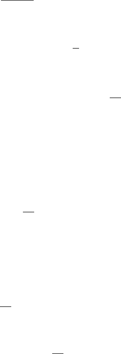
Example N1 – exponentially stable system.
Consider
A(t) =
e
−t
−2 2−e
−t
0 e
−t
−2
, C(t) =
1 0
, R(t) = 1.
The corresponding state transition matrix is
Φ(t, t
0
) =
exp(ψ(t, t
0
)) −ψ(t, t
0
) exp(ψ(t, t
0
))
0 exp(ψ(t, t
0
))
with ψ(t, t
0
) , 2(t
0
−t) + e
−t
0
−e
−t
. This system is exponentially stable.
The Riccati equation (11c) is initialized with P (0) = I
2
and the homogenous system (24)
with z(0) = [1, 2]
T
. In Figure 1 are shown the two eigenvalues (equal to the singular values) of
P (t), which are bounded and tend to zero. In Figure 1 is also shown the state vector z(t), which
converges to zero, in theory exponentially (see Theorem 2).
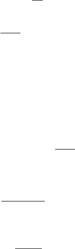
Example N2 – Lyapunov stable system.
Consider
A(t) =
cos(0.2t) sin(0.2t)
− sin(0.2t) cos(0.2t)
,
C(t) =
1.5 0
0 2
, R(t) = I
2
.
16
0 1 2 3 4 5 6 7 8 9 10
−0.5
0
0.5
1
0 1 2 3 4 5 6 7 8 9 10
0
0.5
1
1.5
2
λ
1
(t)
λ
2
(t)
z
1
(t)
z
2
(t)
Figure 1: Example 1. Top: eigenvalues of P (t), bot-
tom: components of z(t).
0 2 4 6 8 10 12 14 16 18 20
−0.5
0
0.5
1
0 2 4 6 8 10 12 14 16 18 20
−0.5
0
0.5
1
1.5
2
λ
1
(t)
λ
2
(t)
z
1
(t)
z
2
(t)
Figure 2: Example 2. Top: eigenvalues of P (t), bot-
tom: components of z(t).
The corresponding state transition matrix is
Φ(t, t
0
) = exp(ϕ(t, t
0
))
cos(ψ(t, t
0
)) sin(ψ(t, t
0
))
− sin(ψ(t, t
0
)) cos(ψ(t, t
0
))
with
ϕ(t, t
0
) , 5(sin(0.2t) − sin(0.2t
0
))
ψ(t, t
0
) , 5(cos(0.2t
0
) − cos(0.2t)).
This system is Lyapunov stable.
The Riccati equation (11c) is initialized with P (0) = I
2
and the homogenous system (24)
with z(0) = [1, 2]
T
. In Figure 2 are shown the two eigenvalues (equal to the singular values) of
P (t), which are bounded and tend to zero. In Figure 2 is also shown the state vector z(t), which
converges to zero, in theory as 1/t (see Theorem 3).
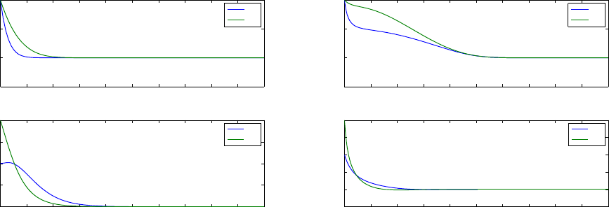
Example N3 – strongly unstable system.
Consider
A(t) =
2−e
−t
e
−t
−2
0 2−e
−t
, C(t) =
1 0
, R(t) = 1.
The corresponding state transition matrix is
Φ(t, t
0
) =
exp(ψ(t, t
0
)) −ψ(t, t
0
) exp(ψ(t, t
0
))
0 exp(ψ(t, t
0
))
with ψ(t, t
0
) , 2(t−t
0
) + e
−t
−e
−t
0
. This system is strongly unstable.
The Riccati equation (11c) is initialized with P (0) = I
2
and the homogenous system (24)
with z(0) = [1, 2]
T
. In Figure 3 are shown the two eigenvalues (equal to the singular values) of
P (t), which are both upper and lower bounded. In Figure 3 is also shown the state vector z(t),
which converges to zero, in theory exponentially (see Theorem 4).
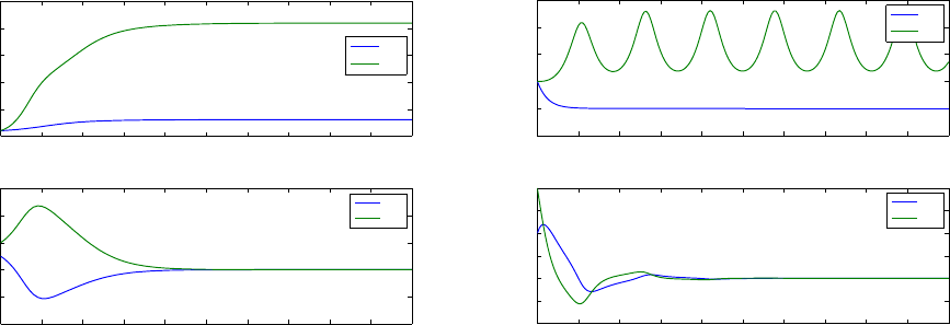
Example N4
Consider
A(t) =
−1 + 1.5 cos
2
t 1 − 1.5 sin t cos t
−1 − 1.5 sin t cos t −1 + 1.5 sin
2
t
,
17
0 1 2 3 4 5 6 7 8 9 10
0
5
10
15
20
25
0 1 2 3 4 5 6 7 8 9 10
−4
−2
0
2
4
6
λ
1
(t)
λ
2
(t)
z
1
(t)
z
2
(t)
Figure 3: Example 3. Top: eigenvalues of P (t), bot-
tom: components of z(t).
0 2 4 6 8 10 12 14 16 18 20
−1
0
1
2
3
4
0 2 4 6 8 10 12 14 16 18 20
−1
−0.5
0
0.5
1
1.5
2
λ
1
(t)
λ
2
(t)
z
1
(t)
z
2
(t)
Figure 4: Example 4. Top: eigenvalues of P (t), bot-
tom: components of z(t).
C(t) =
1 0
, R(t) = 1.
The corresponding state transition matrix is
Φ(t, 0) =
e
0.5t
cos t e
−t
sin t
−e
0.5t
sin t e
−t
cos t
.
This system is neither stable nor strongly unstable.
The Riccati equation (11c) is initialized with P (0) = I
2
and the homogenous system (24)
with z(0) = [1, 2]
T
. In Figure 4 are shown the two eigenvalues (equal to the singular values) of
P (t), which are bounded. In Figure 4 is also shown the state vector z(t), which converges to
zero. No exponential or polynomial convergence rate is theoretically known in this case, but the
result on asymptotic convergence (see Theorem 1) does apply here.
8. Conclusion
For any recursive algorithm running continuously in real time, the boundedness of all the
involved variables is obviously an important property. It is established in this paper that, when
the Kalman filter is applied to OE systems, the solution of the Riccati equation and the Kalman
gain are both bounded, essentially under the observability condition. It is further shown that
the Kalman filter is asymptotically stable, with exponential or polynomial convergence rate in
typical situations. These results complement the classical results on the stability of the Kalman
filter, which do not cover the case of OE systems.
The absence of process noise in OE systems caused a technical difficulty: unlike in the
classical case, here the solution of the Riccati equation does not always have a strictly positive
definite lower bound, therefore the associated “natural” Lyapunov function cannot be used in
the usual sense in the convergence proofs. Despite this difficulty, the results of this paper show
that, the essential condition ensuring the stability of the Kalman filter for OE systems is the
uniform complete observability.
The Kalman filter is optimal in the sense of minimal error covariance. Reducing process
and output noises generally leads to smaller error covariance, including the case of zeroing the
process noise. However, the reduction of error covariance may not be in favor of the average error
convergence, in particular when the process noise is totally absent. In some cases considered in
18

this paper, exponential convergence is not guaranteed, but not explicitly excluded either. This
point still needs investigations in future studies.
Appendix – Proof of Lemma 1
First prove kMk ≤ ξ ⇒ kM vk ≤ ξkvk.
By basic properties of the matrix spectral norm, suppose kMk ≤ ξ, then
kMvk ≤ kMkkvk ≤ ξkvk.
Now let us prove the converse.
Suppose kMvk ≤ ξkvk for all v ∈ R
n
, then by the definition of the matrix spectral norm,
kMk = max
kvk=1
kMvk (72)
≤ max
kvk=1
ξkvk (73)
= ξ. (74)
References
Anderson, B. D., , Bitmead, R. R., Johnson, C. R. J., Kokotovic, P. V., Kosut, R. L., Mareels, I. M.,
Praly, L., Riedle, B. D., 1986. Stability of adaptive systems: passivity and averaging analysis. Signal
processing, optimization, and control. MIT Press, Cambridge, Massachusetts.
Anderson, B. D. O., Moore, J. B., 1979. Optimal Filtering. Prentice-Hall, Inc., New Jersey.
Arnold, W. F., Laub, A. J., 1984. Generalized eigenproblem algorithms and software for algebraic Riccati
equations. Proceedings of the IEEE 72 (12), 1746–1754.
Choi, J., 2010. Linear systems and controls. Lecture notes, http://www.egr.msu.edu/classes/me851/jchoi
/lecture/index.html.
Delyon, B., 2001. A note on uniform observability. IEEE Transactions on Automatic Control 46 (8),
1326–1327.
Forssell, U., Ljung, L., 2000. Identification of unstable systems using output error and box–jenkins model
structures. IEEE Transactions on Automatic Control 45 (1), 137–141.
Goodman, D. M., Dudley, D. G., 1987. An output error model and algorithm for electromegnetic system
identification. Circuits Systems Signal Process 6 (4), 471–505.
Grewal, M. S., Andrews, A. P., 2015. Kalman Filtering: Theory and Practice with Matlab, 4th Edition.
Wiley-IEEE Press.
Ioannou, P., Sun, J., 1996. Robust Adaptive Control. Prentice Hall, electronic copy http://www-
rcf.usc.edu/∼ioannou/Robust Adaptive Control.htm.
Jazwinski, A. H., 1970. Stochastic Processes and Filtering Theory. Academic Press, New York and Lon-
don.
Kalman, R. E., 1963. New methods in Wiener filtering theory. In: Bogdanoff, J. L., Kozin, F. (Eds.),
Proceedings of the First Symposium on Engineering Applications of Random Function Theory and
Probability. John Wiley & Sons, New York, pp. 270–388.
19
Kim, P., 2011. Kalman Filter for Beginners: with Matlab Examples. CreateSpace.
Laub, A. J., 1979. A Schur method for solving algebraic Riccati equations. IEEE Transactions on Auto-
matic Control AC-24 (6), 913–921.
Ljung, L., 1999. System Identification: Theory for the User, 2nd Edition. PTR Prentice Hall, Upper
Saddle River, NJ, USA.
Ni, B., Zhang, Q., July 2013. Kalman filter for process noise free systems. In: IFAC International Work-
shop on Adaptation and Learning in Control and Signal Processing (ALCOSP). Caen, France.
Ni, B., Zhang, Q., 2015. Stability of the Kalman filter for output error systems. In: Submitted to the
17th IFAC Symposium on System Identification. Beijing.
Pengov, M., Richard, E., Vivalda, J.-C., 2001. On the boundedness of the solutions of the continuous
Riccati equation. Journal of Inequalities and Applications 6 (6), 641–649.
Rugh, W. J., 1995. Linear System Theory. Prentice Hall.
Sastry, S., Bodson, M., 1989. Adaptive Control: Stability, Convergence and Robustness. Prentice-Hall.
Wang, L., Ortega, R., Su, H., Liu, Z., Liu, X., 2015. A robust output error identifier for continuous-time
systems. International Journal of Adaptive Control and Signal Processing 29 (4), 443–456.
Zarchan, P., Musof, H., 2005. Fundamentals of Kalman filtering: a practical approach. AIAA.
Zhang, L., Zhang, Q., 2015. Observability conservation by output feedback and observability Gramian
bounds. Automatica 60, 38–42.
URL https://hal.inria.fr/hal-01231786
20
