Performance Analysis and Non-Quadratic Lyapunov Functions for

arXiv:2009.00727v2 [eess.SY] 11 Sep 2020

Linear Time-Varying Systems

Matthew Abate, Corbin Klett, Samuel Coogan, and Eric Feron

Abstract— Performance analysis for linear time-invariant

(LTI) systems has been cl osely tied to quadratic Lyapunov

functions ever since it was shown that LTI system stability is

equivalent to the existence of such a Lyapunov function. Some

metrics for LTI systems, however, have resisted treatment via

means of quadratic Lyapunov functions. Among these, point-

wise-in-time metrics, such as peak norms, are not captured

accurately using these techniques, and this shortcoming has

prevented the development of tools to analyze system behavior

by means other than e.g. time-domain simulations. This work

demonstrates how the more general class of homogeneous poly-

nomial Lyapunov functions can be used to approximate point-

wise-in-time behavior for LTI systems with greater accuracy,

and we extend this to the case of linear time-varying (LTV)

systems as well. Our ﬁndings rely on th e recent observation that

the search for homogeneous polynomial Lyapunov functions for

LTV systems can be recast as a search for quadratic Lyapunov

functions for a related hierarchy of time-varying Lyapunov

differential equations; thus, performance guarantees for LTV

systems are attainable without heavy computation. Numerous

examples are provided to demonstrate the ﬁndings of this work.

I. INTRODUCTION

Beginner’s courses on linear systems quickly introduce the

Lyapunov function as a natur al means to expre ss system

stability in terms of energy lo ss. O ne essential result of

Lyapunov states that the stability of a linear time invariant

(LTI) system is equ ivalent to the existence of a quadratic

energy function that decays along system trajector ie s [1],

and since then qua dratic stability theory has been greatly

extended to develop metrics and indicators of performance

such as passivity [2, Chapte r 14], [3] and robustness [4].

These metrics generally leverage the ubiq uitous presence of

the quadratic Lyapunov functions that are n a turally embed-

ded in stable LTI systems [5].

Some metric s for LTI systems, however, have resisted

treatment via means of quadra tic Lyapunov functions.

Among these, poin t-wise-in-time metrics, such as peak

norms, are not captured accurately [6], and this shortcoming

has prevented the development of tools to analyze system

behavior by me a ns oth er than time-domain simulations.

This work was supported by the KAUST baseline budget.

M. Abate is with the School of Mechanical Engineering and the School

of Electrical and Computer Engineering, Georgia Institute of Technology,

Atlanta, 30332, USA: Matt.Abate@GaTech.edu.

C. Klett is with the School of Aerospace Engineering, Georgia Institute

of Technology, Atlanta, 30332, USA: [email protected].

S. Coogan is with the School of Electrical and Computer Engineering

and the School of Civil and Environmental Engineering, Georgia Institute

of Technology, Atlanta, 30332, USA: [email protected]u.

E. Feron is with the Department of Electrical Engineering, King Ab-

dullah University of Science and Technology, Thuwal, Saudi Arabia:

Eric.Feron@Kaust.edu.sa.

When extending to the case of linear time-varying (LTV)

systems, new cha llenges emerge: for instance, it is known

that not a ll stable LTV systems c an be certiﬁed v ia quadratic

Lyapunov functions [7], and the time-varying na ture of these

systems reduces the ease of simulation. Fur ther, analytical

considerations in simulation are often steere d by subjective

criteria: for example, the stopping-time of a simulation is, in

practice, generally chosen by either analysing the poles of

the system or the relative distance to the steady-state output

(See, e.g. [8, impulse.m]). For these reasons, it is useful to

have means other than simulation for extracting time domain

properties f or LTV systems.

The topic addressed in this paper relies on the re cent ob-

servation in [9] that the search for homogene ous polynomial

Lyapunov functions for LTV systems can be recast as the

search for quadratic Lyapunov fun ctions for a related hierar-

chy of Lyapunov differential equa tions. Indeed, every stable

LTV system induces a h omogeneous polynomial Lyapunov

function [10], [11], and the search for such a Lyapunov

function is easily expr essed as sum-of-squares and foun d

by solving a convex, semi-deﬁnite feasibility program. Our

contribution is to show that the aforementioned hierarchy

of LTI systems deﬁnes a p owerful framework for extracting

time-dom ain properties of LTV systems, a nd we particularly

show how one can compute bounds on the impulse an d step

response of LTV systems using homoge neous polynomial

Lyapunov functions.

This paper is structured as follows. We in troduce our

notation in Section II. In Section III we recall a procedure

for computing norm bounds on the impulse response of LTI

systems, and this procedure relies on the use of quad ratic

Lyapunov functions. In the same section, we introduce a

hierarchy of LTI systems that can be used to compute homo-

geneous polynomial Lyapunov functions for LTI systems. We

show how th e afor ementioned hierarchy is used to compute

bounds on the impulse responses of LTI systems in Section

IV and bo unds on the step responses of LTI systems in

Section V. Similar bounds are co mputed for LTV systems

in Section VI, and we additionally present a procedure for

computing convergence envelopes on the impulse response of

LTV systems. We demonstrate our ﬁndings through numer-

ous examples that appear througho ut the work and through

a case study presented in Section VII.

II. NOTATION

We denote by S

⊂ R

n×n

the set of symmetric positive

deﬁnite n ×n matr ices. We denote by I

the n ×n identity

matrix, and we denote by 0

∈ R

the zero vector in R

Given A ∈ R

n×m

and integer i ≥ 1, we denote by ⊗

A ∈

×m

the i

-Kronecker Power of A, as deﬁned recursively

⊗

A := A

⊗

A := A ⊗ (⊗

i−1

A) i ≥ 2.

(1)

III. PRELIMINARIES

We consider th e linear time-invariant system

˙x = Ax + bu,

y = cx,

(2)

with state x ∈ R

, control input u ∈ R and output y ∈ R. We

are particularly interested in studying the impulse response

of (2), which is given by

h(t) = ce

b. (3)

Elementary simulations may provide desired information

such as a no rm-bound on h(t). However, such simulations

become cumbersome and inelegant when e.g. A, b, or c

are unc ertain or time-varying. To address these r obustness

issues, algebraic approaches to time-domain analyses have

been proposed that rely on quadratic Lyapunov functions [3,

Section 6.2], [12].

A quad ratic Lyapunov function for (2) is given by V (x) =

P x where P ∈ S

satisﬁes

P + P A  0. (4)

Indeed , any quadratic Lyapunov function for (2) implicitly

deﬁnes an ellipsoidal sublevel set



x ∈ R

and x

P x ≤ α



(5)

for any positive α, and this sublevel set is invariant in the

sense tha t any trajec tory of ˙x = Ax th at starts within E

stays within E

for all time. Based on this consideration, an

upper bound on the impulse response may be obtained from

any invariant ellipsoid, as we show in Proposition 1.

Proposition 1. [3] If P ∈ S

satisﬁes (4), then |h(t)|≤

for all t ≥ 0 where

h =

√

−1

√

P b. (6)

Proof. Let α = b

P b. Then a norm bound on h(t) can be

computed by ﬁnding the point on the boundary of E

in the

direction c; that is |h(t)|≤

h for all t, where h is given by

h = max

z∈R

s.t. z

P z ≤ b

P b

(7)

and this optimization problem is solved by (6).

To ﬁnd the ellipsoid parameter P which minimizes the

bound on the impulse respon se while satisfying the Lyapunov

constraint (4), we formulate the program

P = arg min

Q∈S

−1

s.t. b

Qb ≤ 1

Q + P Q  0

(8)

which can be easily computed via convex optimization

techniques (See Exam ple 1)

Example 1. Consider the system

˙x =



0 1

−1 −0.9



x +





u, (9)

y =

√

2 −

√



Solving (8), we have that P = (0.5)I

is the ellipsoid al

parameter that minimizes impulse response bound given in

(6). T hen, from (6) we ﬁnd |h(t)| ≤

h = 2

√

2 for all t.

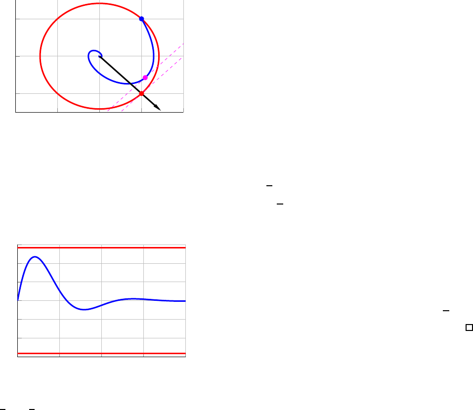
Figures 1a and 1b plot the impulse response of (9) in the

phase plane and time domain, re spectively. 

The maximum impulse response of a passive system is

known to be equal to h from (6) [3], however, the norm

bound (6) generally suffers from conservatism (See Example

2).

Example 2. Consider the system (2) with stiff dynamics

(A)

i, j

(

−(M )

i−1

if i = j

0 otherwise,

(b)

= 1

(c)

(

1 if i = 1

(−1)

i+1

2 otherwise.

for some M ≥ 0. This system is stable, and |h(t)|≤ 1 for all

t ≥ 0. However, it was shown in [14] that the gap between

the actual maximum impulse response and the upper bound

obtained by solving (8) grows to 2n − 1 when M tends

toward inﬁnity. 

In this work, we a ddress the aforeme ntioned conservatism,

and we present a similar technique for generating a norm

bound on h(t) that relies on nonquadratic Lyapunov func-

tions for the system ˙x = Ax. To that end, we ﬁrst deﬁne the

following inﬁnite hierarchy o f LTI systems:

(

= A

(

= A

= I

⊗ A

i−1

+ A ⊗ I

i−1 , i ≥ 2,

(10)

where A ∈ R

n×n

and the state of the system H

is given

by ξ

∈ R

. This hierarchy is best un derstood by looking

at H

, wh ic h is the vectorized version o f the Lyapunov

differential equatio n

X = AX + XA

with X ∈ R

n×n

Moreover, if x(t) is a solution to ˙x = Ax then ξ

(t) =

(⊗

x(t)) is a solution to H

. This hierarchy is closely

tied to the Liouville equations u sed to obtain the inﬁnite-

dimensional linear differential equations which drive the

evolution of p robability density functions, in a way similar to

In Example 1, and those that follow, we compute (8) using CVX [13],

a convex optimization toolbox, made for use with MATLAB. The code that

generates the ﬁgures from these examples is publicly available through the

GaTech FactsLab GitHub: https://github.com/gtfactslab/Abate

ACC2021

−2 −1 0 1 2

−1

(a) Phase portrait of the impulse response for the system (9). The

impulse response of (9) is shown i n blue, and x(0) = b is shown

as a blue dot. The vector c

is shown with a black arrow, and the

state along x (t) w hich maximizes h(t) is shown as a pink dot.

The invariant ell ipse E

is shown in red and the vector z which

solves (7) is shown as a red dot. The two dashed lines depict a

“gap” of conservatism between the bound produced by E

and the

actual maximum impulse response.

0 3 6 9 12

−3

−2

−1

h(t)

(b) Impulse response for the system (9), plotted in the time domain.

The impulse response of (9) is shown in blue, and the magnitude

bound

h = 2

√

2 is shown in red.

Fig. 1: Example 1. Figures 1a and 1b plot the impulse

response of the system (9) in the phase plane and time

domain, resp e ctively.

the Chapman-Kolmogorov equations [15, Chapter 16]. See

also [16] for the discrete-tim e parallel to (10).

An essential observation made in [9] is that a quadratic

Lyapunov function for the i

level system H

identiﬁes a

homogeneous polynomial Lyapunov fu nction for ˙x = Ax;

that is, if P

∈ S

satisﬁes

+ P

 0 (11)

for A

as deﬁned in (10), then a polynomial Lyapunov

function for the system ˙x = Ax is given by

V (x) = (⊗

(⊗

x) (12)

and this Lyapunov function is homogen e ous in the entries of

x and is of order 2i.

IV. IMPULSE RESPONSE ANALYSIS VIA HOMOGENEOUS

POLYNOMIAL LYAPUNOV FUNCTIONS

Our main result is to show that the impulse response

bound on h(t), which is provided in Proposition 1, can

be considerably improved when hig her-order polynomial

Lyapunov functions are consid ered. I n particular, we study

the guaran te e s attainable when considering th e h omogeneous

polynomial Lyapunov functions that naturally arise from the

hierarchy of stable LTI systems (10), and we show in the

following theorem how these Lyapunov functions are used

to b ound the impulse response h (t).

For integer i ≥ 1, deﬁne b

∈ R

and c

∈ R

= ⊗

b, c

= ⊗

Theorem 1. If P

∈ S

satisﬁes (11) at the i

level, then

|h(t)| ≤

h for all t where

h = (c

−1

)

1/(2i)

)

1/(2i)

. (13)

Proof. For any integer i ≥ 1, construct the system

ξ = A

ξ + b

y = c

(14)

with ξ ∈ R

, u ∈ R, and impulse response h(t). Assuming

∈ S

satisﬁes (11) at the i

level, we have that

|h(t)|≤ (c

−1

)

1/2

)

1/2

. Moreover, f rom the

construction (14), we have that |h(t)|≤ |h(t)|

1/i

h. Th is

competes the proof.

As in (8), we next formulate a convex program to search

for the parameter P

which provides the tightest upper bound

on h(t) attainable using Theorem 1:

= arg min

Q∈S

−1

s.t. b

≤ 1

Q + QA

 0.

(15)

We demonstrate the application of Theorem 1 in Example 3.

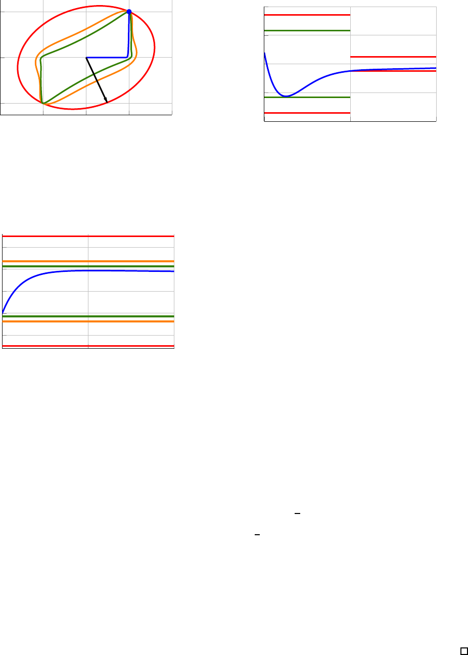
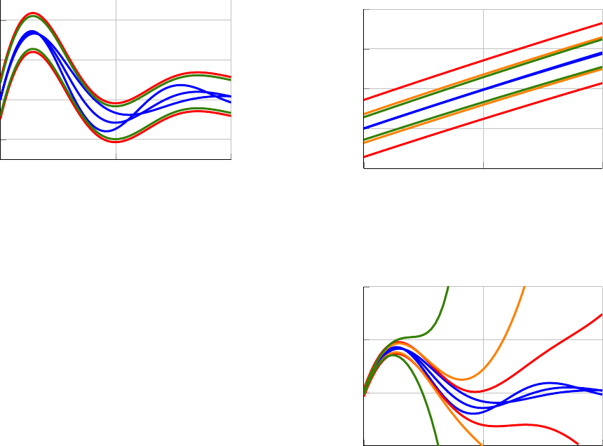
Example 3. We consider the stiff system, previously pre-

sented in Example 2, where we take n = 2 and M = 100.

The optimization pro blem (15) is solved for i = 1, 2, 5,

and the resulting qu adratic Lyapunov parameters P

are used

to generate bounds on the impulse response using (13). In

Figure 2, we show the impulse response of the stiff system

and the bounds derived using Theorem 1. Note that as the

degree of the Lyapunov functions grows, the sublevel sets

of the resulting Lyapunov function shrink and approximate

the relevant parts of the impulse response trajectory in the

state-space with greater accur a cy. 

As illustrated in Example 3, the accuracy of the bound

(13) will generally increase as i increases. This is due to the

fact that the homogeneou s polynomial Lyapunov functions

generalize quadratic Lyapunov functions [9].

Theorem 1 can also be used to reduce the simulation

complexity for systems of the fo rm (2). While it is nat-

ural to analyse such systems though simulation, it c an be

−2 −1 0 1 2

−1

(a) Phase portrait of the impulse response for the stiff system

from Example 2 where n = 2 and M = 100. The impulse

response is shown in blue, and x(0) = b is shown as a blue dot.

A vector in the direction of c

is shown with a black arrow. The

invariant sublevel sets of the 2

, 4

and 10

order homogeneous

polynomial Lyapunov functions that are derived in this study are

shown in red, orange and green, respectively.

5 ·10

−2

0.1

−2

−1

h(t)

(b) Impulse response for the system (9), plotted in the time domain.

The impulse response of (9) is shown in blue, and the magnitude

bounds derived using P

for i = 1, 2, 5 are shown in red, orange

and green, respectively. As t goes to inﬁnity, h(t) decays to 0.

Fig. 2: Example 3. Figures 2a and 2b plot the impulse

response of the stiff system from Example 2, where n = 2

and M = 100.

ambiguous as whe n a simulation should be stopped. I n the

following example, we demonstrate one potential solution to

this problem, wh ereby a system is simulated over a given

amount of time and then the remaining simulation output is

bounded using (13).

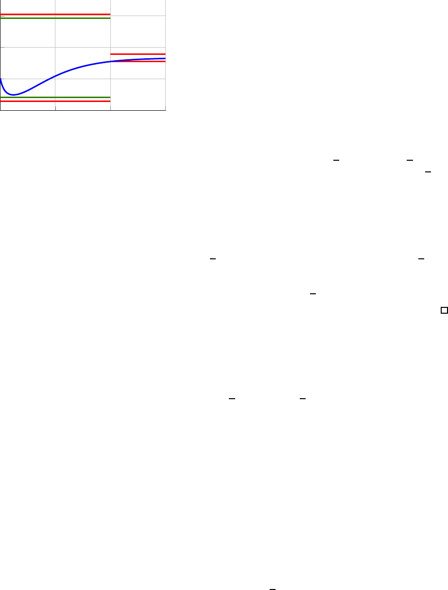
Example 4. Consider the system (2) with x ∈ R

and

A =





0.3 0.5 10

−1 −1.7 1

−2 −2 −7.7





, b =





0.2





, c





−2





The optim ization problem (15) is solved for i = 1, 4, and

the resulting Lyapunov para meters P

are used to generate

bounds on the impulse response using (13). At time t = 1, a

new bound is computed via (13) wh e re b is now taken to be

the simulated state x(1); this creates a norm bound on the

tail of the impulse response, as shown in Figur e 3. 

0 1 2

−1

−0.5

0.5

h(t)

Fig. 3: Example 4. The impulse response h(t) is shown in

blue, and the magnitu de bounds derived using P

and P

are shown in red and green, respectively. At time t = 1, a

bound on the tail of h(t) is computed via (13) with i = 1,

and this bound is shown in red.

V. STEP RESPONSE ANALYSIS VIA HOMOGENEOUS

POLYNOMIAL LYAPUNOV FUNCTIONS

We next turn our discussion to the step response of (2),

which is the output y(t) w hen x(0) = 0

and u(t) = 1 for

all t ≥ 0. Equivalently, the step response of (2) is given by

s(t) where

˙x = Ax + b

s = cx

(16)

and x(0) = 0

, and a closed form representation of the step

response is given by

s(t) = cA

−1

− I

)b. (17)

As we show next, a norm bound on s(t) can be de rived

using Lyapunov functions in manner similar to that pr esented

previously. For integer i ≥ 1, deﬁne A

∈ R

×n

= ⊗

−1

Theorem 2. If P

∈ S

satisﬁes (11) at the i

level, then

|s(t) + cA

−1

b| ≤

s for all t wh e re

s = (c

−1

)

1/(2i)

)

1/(2i)

. (18)

Proof. The system (16) has a stable equilibrium x

−A

−1

b. Taking the tran sformation ex(t) = x(t) − x

, we

ﬁnd that the step response of (2) is equal to the impulse

response of the system

ex = Aex + A

−1

y = cex − cA

−1

(19)

Thus, the bound (18) is derived using The orem 1.

Using sim ilar reason ing to that of (8), we ﬁnd that the

Lyapunov parameter P

that provides the tightest upper

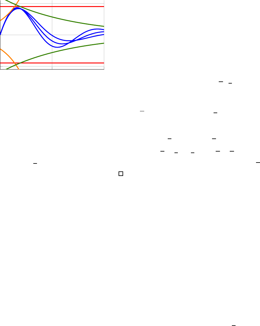
0 2 4 6

−0.5

0.5

h(t)

Fig. 4: Example 5. Th e step response s(t) is shown in blue,

and the magnitude bounds derived u sing the P

for i = 1, 3

are shown in red and green, respectively. At time t = 1, a

new bound is computed via (1 8) using i = 1 and this bou nd

is shown in red.

bound on |s(t)+cA

−1

b| attainable using Theorem 2 is given

P = arg min

Q∈S

−1

s.t. b

≤ 1

Q + QA

 0.

(20)

We demonstrate the application of Theorem 2 in Example 5.

Example 5. Consider the system (2) with x ∈ R

and

A =





−1 0 2

0 −10 1

0 −2 −1





, b =





−2





, c





−2





The optim ization problem (20) is solved for i = 1, 3, and

the resulting Lyapunov para meters P

are used to generate

bounds on the step response using (18). At time t = 4, a

new bound on th e step response is computed v ia (18), and

this creates a norm bound on the tail of s(t), as shown in

Figure 4. 

VI. IMPULSE RESPONSE ANALYSIS FOR LINEAR

TIME-VARYING SYSTEMS

The foregoing ideas can be used over a range of po ssible

applications going beyond the ana lysis of a single LTI sys-

tem. Lyapunov functions have long been known to be useful

for robustness analyses, and we explore these applications in

this section.

A. Bounds on Impulse Response for Uncertain and Nonlin-

ear Systems

The foregoing bounds on impulse re sponse can be rea dily

extended to the case of linear time-varying input-o utput

systems. Spec iﬁca lly, we consider

˙x = A(t)x + bu,

y = cx,

(21)

where for given A, ∆ ∈ R

n×n

, we have that

A(t) ∈

A + λ∆ |λ ∈ [−1, 1]

(22)

for all t. In this case, the impulse response h(t) is described

parametrica lly b y a solu tion ϕ(t) to

˙ϕ(t) = A(t)ϕ(t)

h(t) = cϕ(t)

ϕ(0) = b.

(23)

Theorem 3 shows how a norm bound on h(t) for (21) can

be similarly computed b y considering the hierarchy (10).

Theorem 3. If P

∈ S

satisﬁes (11) for A+∆ and A−∆

at the i

level, then |h(t)| ≤

h for all t where h is given

by ( 13). Moreover, the parameter P

which minimizes h can

be computed with (8), where P

is understood to satisfy (11)

for both A + ∆ and A − ∆ at the i

level.

Proof. Assume there exists a P

∈ S

that satisﬁes (11) for

both A+∆ and A−∆ at the i

level. Then, the system ˙x =

A(t)x is stable with a homogeneous polynomial Lyapunov

function V (x) = (⊗

(⊗

x) [9]. Therefore |h(t)| ≤

h, where h(t) is the impulse response of (21) and h the a

point on the level set {x ∈ R

|V (x) = b

} in the

direction c

. It follows from the reaso ning presented in the

proof of Theorem 1 that

h is given by (13). This completes

the proof.

The stability guarantees in Theorem 3 are in terms of a

global norm bound on h(t). We next generalise Theo rem

3 to provide a time-dependent bound on h(t) which is

exponentially growing/decaying in t (See Theorem 4).

Theorem 4. For α ∈ R, if P

∈ S

satisﬁes (11) for

A +∆+αI

and A−∆+αI

at the i

level, then |h(t)| ≤

−αt

h for all t where h is g iv e n by (13).

Proof. Choose α ∈ R, and assume there exists a P

∈ S

that satisﬁes (11) for both A +∆+αI

and A−∆+αI

at the

level. Then, V (x) = (⊗

(⊗

x) is a homogeneous

polynomial Lyapunov functio n f or the system

˙x = A

(t)x. (24)

where A

(t) ∈ R

n×n

evolves according to

(t) ∈

A + αI

+ λ∆



λ ∈ [−1, 1]

. (25)

Thus, applyin g the results of Theorem 3, we have that the

impulse response of

˙x = (A(t) + αI

)x + bu

y = cx

(26)

is bounded by

h fr om (13).

Fix an A(t) satisfying (22), and denote by ϕ(t) ∈ R

h(t) ∈ R the solutio n to (23). Then ϕ

(t) := e

αt

ϕ(t) is the

solution to

˙ϕ

(t) = (A(t) + αI

)ϕ

(t)

(0) = b.

(27)

0 5 10

−1

h(t)

Fig. 5: Example 6. Thre e system simulations are conducted,

and the impulse responses of each is plotted in blue. A global

norm bound on h(t) is computed using Theorem 3 for i = 6,

and this bound is shown in red. Two exponential bounds on

h(t) are constructed fro m Theorem 4 with α = −0.5, 0.15

and i = 6, and the boun ds are shown in oran ge and gree n,

respectively.

Therefore |h(t)| ≤ e

−αt

h for all t. This completes the proof.

We demonstrate application of Theorems 3 and 4 in

Example 6.

Example 6. Consider the uncertain system (21) with x ∈ R

and

A =



0 1

−0.6 −0.5





0 1



∆ =



0 0

0.1 −0.1



c =



1 0



(28)

The optimization problem (2 0) is solved for i = 6 and

the resulting Lyapun ov parameters P

are used to generate

bounds on the impulse response using (13). Next, Theorem

4 is employed, and exponential stability guarantees are

computed for α = −0.5 , 0.15 and i = 6. The expo nential

and global norm bounds compu ted in this study are shown

in Figure 5 in the tim e domain, along with several sample

system impulse responses. 

B. Robust Uncertain System Simulation

As demonstrated in the previous example s, the b ound

provided in (13)—which is introduced in Theorem 1 and

generalised in Theorem 3—will generally only serve as a

good approximation of the sy stem response initially. Thus,

the bound provided in (13) may be too weak to employ in

instances where, e.g., long-term system knowledge is neede d,

and we have attempted to address this concern by providing

e.g. norm- bounds on the tail of the impulse response (See

Examples 4 and 5), and exponential stability bounds (See

Theorem 4 and Example 6). As an alternative, we next

present a method for approximating h(t) for (21) that uses

the difference between the impulse responses within a family

of linear systems.

We consider

ex =



A(t) 0

0 A



ex +





y =



c −c



ex,

(29)

and where A(t) satisﬁes (22). Given a signal A(t), we have

that the impulse response of (29) is equal to h(t) − ce

where h(t) is the im pulse re sponse of (21) and is given by

(23). Th us, a new tim e varying bound on h(t) can be d erived

straightfor ward ly from the results presented previously (See

Theorem 5).

Deﬁne A

, A

−

∈ R

2n×2n

, and

, c

∈ R

(2n)



A + ∆ 0

0 A



, A

−



A − ∆ 0

0 A



= (⊗



1 1



)

⊗ b, c

= (⊗



1 −1



) ⊗ c.

Theorem 5. For α ∈ R, if P

∈ S

(2n)

satisﬁes (11) for

+ αI

and A

−

+ αI

at the i

level, then |h(t) −

b| ≤ e

−αt

h for all t where h is g iv e n by

h = (c

−1

)

1/(2i)

)

1/(2i)

. (30)

Moreover, the pa rameter P

which minimizes

h can be

computed with (8), where P

is understood to satisfy (11)

for both A

+ αI

and A

−

+ αI

at the i

level.

The applicatio n of Theorem 5 is demonstrated through a

case study in th e following section.

VII. NUMERICAL EXAMPLE

In this study we consider the uncertain linear system (21)

previously introduced in Example 6, and restated here: we

consider (21) with x ∈ R

and

A =



0 1

−0.6 −0.5





0 1



∆ =



0 0

0.1 −0.1



c =



1 0



(31)

We ﬁrst consider the case where α = 0. We compute P

and P

that satisﬁes the hypothesis of Theor em 5 using (8).

By applying Theorem 5, we compute an envelope centered

at ce

b which contains the impulse response of ( 21). The

bounds computed in this study are shown in Figure 6, plotted

in the time domain.

We next con sid er the case where α < 0. I n this case, the

envelope

|h(t) − ce

b| ≤ e

−αt

h, (32)

that bounds the impulse response h(t) will grow with

time. We demonstrate this assertion by computing P

∈

(2n)

that satisﬁes the hypothesis of Theorem 5 for α =

−0.25, −0.5, −1, and plotting the re sulting convergence en-

velopes (See Figure 7). Note that as α decreases the envelope

bound (32) will approx imate the in itial system behavior with

greater accuracy; however, the long-ter m accuracy is better

achieved with higher values α.

Finally, we consider the case wh e re α > 0 and, in

this case, the resulting envelope (32) will shrink with time.

Moreover, this bound will converge more quickly when α is

0 6 12

−0.5

0.5

h(t)

Fig. 6: Three system simulations are conducted, and the

impulse responses of each is plotted in blue. Two envelope

bounds on h(t) are computed using Theorem 5 with α = 0

and i = 1, 3, and these envelope bounds are shown in r ed

and green, respectively.

large and this bound will increase in accuracy as the order

of the search i inc reases. To demonstrate this assertion we

compute P

that satisﬁes the hypoth e sis of Theorem 5 for

α = 0.1 at the levels i = 1, 3. The resulting convergence

envelopes are shown in Figu re 8a; note that as i increases,

the bound (32) approximates the true maximum impulse

response of (21) with gr eater ac curacy. Additionally, we ﬁnd

that as the order of the search i increases, higher α values

are possible. For instance, when searching for a quadratic

Lyapunov parameter P

that satisﬁes the hypothesis of The-

orem 5, the optimization problem (8) is solvable only when

α ≤ 0.156. However, at the i = 2 level the optimization

problem (8) is solvable for α ≤ 0.169, and at the i = 3 level

the optimization problem ( 8) is solvable for α ≤ 0.173. The

envelope bounds derived from these maximum α parameters

are shown in Figure 8b.

VIII. CONCLUSION

This work demonstrates how the more general class of

homogeneous polynomial Lyapunov functions can be used to

approximate p oint-wise-in-time behavior for LT V systems,

and we particularly study the im pulse and step response

of these systems. Our ﬁndings rely on the recent observa-

tion that the search for homogeneous polynomial Lyapunov

functions for LTV systems can be recast a s a sear ch for

quadra tic Lyapunov functio ns for a related h ie rarchy of time-

varying Lyapunov differential equations; thus, performance

guaran tees for LTV systems are attainable without heavy

computation. Num erous examples are provided to demon-

strate the ﬁndings of this work.

REFERENCES

[1] H. K. Khalil and J. W. Grizzle, Nonlinear systems, vol. 3. Prentice

hall Upper Saddle River, NJ, 2002.

[2] W. J. Terrell, Stability and stabilization: an introduction. Princeton

University Press, 2009.

[3] S. Boyd, L. El Ghaoui, E. Feron, and V. Balakrishnan, Linear matrix

inequalities in system and control theory. SIAM, 1994.

0 0.1 0.2

−0.1

0.1

0.2

0.3

h(t)

(a) Short time scale: as α ≤ 0 decrease, the envelope bound (32)

approximates the impulse response of (21) with greater accuracy

on short time horizons.

0 6 12

−1

h(t)

(b) Long time scale: as α ≤ 0 increases, the envelope bound (32)

approximates the impulse response of (21) with greater accuracy

on long time horizons.

Fig. 7: Three system simulations are conducted an d the

impulse response of each is plotted in blue. Three conference

envelopes are formed by applying the procedu re detailed in

Theorem 5 at level i = 2. We compute P

∈ R

using (8)

for α = −0.25, −0.5, −1, and the resulting envelope bounds

(32) are shown in red, orange and green, respectively.

[4] K. Zhou and J. C. Doyle, Essentials of robust control, vol. 104.

Prentice hall Upper Saddle River, NJ, 1998.

[5] C. Hollot and B. Barmish, “Optimal quadratic stabilizability of uncer-

tain linear systems,” in Proc. 18th Allerton Conf. on Communication,

Control and Computing, pp. 697–706, University of Illinois, 1980.

[6] F. Blanchini, “Nonquadratic lyapunov functions for robust control,”

Automatica, vol. 31, no. 3, pp. 451–461, 1995.

[7] D. Liberzon, Switching in systems and control. Springer Science &

Business Media, 2003.

[8] MATLAB, version 9.8 (R2020a). Natick, Massachusetts: The Math-

Works Inc., 2020.

[9] M. Abate, S. Coogan, and E. Feron, “Lyapunov differential equation

hierarchy and polynomial lyapunov functions for switched linear

systems,” in 2020 American Control Conference, pp. 5322–5327,

IEEE, 2020. An extended version of this work appears on ArXiv:

https://arxiv.org/abs/1906.04810.

[10] P. Mason, U. Boscain, and Y. Chitour, “Common polynomial lyapunov

functions for linear switched systems,” SIAM journal on control and

optimization, vol. 45, no. 1, pp. 226–245, 2006.

[11] A. A. Ahmadi and P. A. Parrilo, “Converse results on existence of

sum of squares lyapunov functions,” in 2011 50th IEEE conference

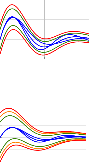
0 6 12

−0.75

0.75

1.5

h(t)

(a) Three envelope bounds are formed by applying the procedure

detailed in Theorem 5 at levels i = 1, 3 with α = 0.1. These

bounds are shown in red and green, respectively.

0 6 12

−2

−1

h(t)

(b) Three envelope bounds are formed by applying the procedure

detailed in Theorem 5. The i = 1

order envelope bound formed

by solving (8) with α = 0.156 is shown in red. The i = 2

order

envelope bound formed by solving (8) with α = 0.169 is shown

in orange. The i = 3

order envelope bound formed by solving

(8) with α = 0.173 is shown in green.

Fig. 8: Three system simulations are conducted an d the

impulse response of each is plotted in blue. Convergence

envelopes are formed by applying the procedu re detailed in

Theorem 5 at level i = 1, 2, 3 for α ≥ 0.

on decision and control and European control conference, pp. 6516–

6521, IEEE, 2011.

[12] J. Abedor, K. Nagpal, and K. Poolla, “A linear matrix inequality

approach to peak-to-peak gain minimization,” International Journal of

Robust and Nonlinear Control, vol. 6, no. 9-10, pp. 899–927, 1996.

[13] M. Grant and S. Boyd, “CVX: Matlab software for disciplined convex

programming, version 2.1.” http://cvxr.com/cvx, Mar. 2014.

[14] E. Feron, “Linear matrix inequalities for the problem of absolute

stability of control systems,” 1994.

[15] G. J. Lieberman and F. S. Hillier, Introduction to operations research.

McGraw-Hill, 8 ed., 2004.

[16] C. Klett, M. Abate, Y. Yoon, S. Coogan, and E. Feron, “Bounding

the state covariance matrix for switched linear systems with noise,” in

2020 Am erican Control Conference, pp. 2876–2881, IEEE, 2020.