
Lecture Week 7: Lyapunov Stability of Linear Time-varying Systems
This week’s lecture has two objectives. The first part of the week extends Lyapunov sta-
bility concepts to linear time-varying (LTV) systems. For such systems, one can no longer
use the eigenvalue conditions or the matrix Lyapunov equation to certify stability. Lya-
punov stability for time-varying systems has to be refined to hold “uniformly” with respect
to the initial time. The second objective of this week’s lecture is to extend stability con-
cepts to forced systems. This leads to the notion of input-output stability that we define
with respect to the L
p
norms of the signal spaces. We examine the relationship between L
p
stability and Lyapunov stability and use this relationship to set up our next topic addressing
the controllability and observability of linear dynamical systems.
Mathematical Preliminaries: Consider a C
1
function v : R → R and let there be a
function f : R → R. The function v is said to satisfy a differential inequality if such that
˙v(t) ≤ f(v(t))
for all t. We can use this relationship to bound the v(t) for all time. In particular, let
x : R → R be a function that satisfies the initial value problem,
˙x(t) = f(x(t)), x(0) = v(0)
Then a result known as the comparison principle allows us to assert that v(t) ≤ x(t) for all
t ≥ 0.
1. UNIFORM STABILITY CONCEPTS
We need to refine the earlier Lyapunov stability concept when it is applied to time-varying
systems. To help illustrate the need for this refinement, consider the LTV system
˙x(t) = (6t sin(t) − 2t)x(t)
One may view this as a linear system, ˙x(t) = a(t)x(t) whose time-varying coefficient a(t)
is subject to a damping force and a sinusoidal perturbation that both grow over time. The
solution may be obtained by first separating the variables, x and t
dx
x
= (6t sin(t) − 2t)dt
1

2
and then integrating both sides of the equation from t
0
(initial time) to t > t
0
assuming
x(t
0
) = x
0
.
x(t) = x(t
0
) exp
Z
t
t
0
(6s sin(s) −2s)ds
= x(t
0
) exp
6 sin(t) −6tcos(t) − t
2
− 6 sin(t
0
) + 6t
0
cos(t
0
) + t
2
0
For a fixed initial time, t
0
, one sees that eventually the quadratic term, t
2
, will denominate
the exponential function’s behavior, thereby implying that the exponential function in the
above equation is bounded above by a function of t
0
, say c(t
0
). It therefore follows that
|x(t)| ≤ c(t
0
)|x(t
0
)|, for all t ≥ t
0
If we then consider any ϵ > 0 and select the initial neighborhood δ(ϵ) =
ϵ
c(t
0
)
then clearly
|x(t)| remains with a ϵ-neighborhood of the equilibrium and so we can conclude the equi-
librium at 0 is stable in the sense of Lyapunov.
The issue we face here, however, is that δ is not just a function of ϵ, it is also a function of
the initial time t
0
. Our worry is that as t
0
→ ∞ that δ(ϵ, t
0
) could approach a finite limit
that is, in fact, zero. If we think of t
0
as the system’s current “age”. Then this says as the
system ages (i.e. t
0
gets larger) our ability to keep |x(t)| < ϵ is harder and harder as we
have to start in a smaller and smaller distance, δ, from the origin.
This is precisely the case with this particular system. In particular, consider a sequence of
initial times {t
0n
}
∞
n=0
where t
0n
= 2nπ for n = 0, 1, 2, . . . , ∞. Let us evaluate x(t) exactly
π time units after t
0n
to see that
x(t
0n
+ π) = x(t
0n
) exp
6(2n + 1)π − (2n + 1)
2
π
2
+ 6(2nπ) + (2n)
2
π
2
= x(t
0n
) exp
24nπ + 6π − 4nπ
2
− π
2
= x(t
0n
) exp {(4n + 1)(6 − π)π}
and for any x(t
0
) ̸= 0 we then can see that the ratio
x(t
0n
+ π)
x(t
0n
)
= e
(6−π)π(4n+1)
= 7942.2e
35.918n
→ ∞
as n → ∞. In other words, as the system ages in the sense that t
0n
goes to infinity, we see
that ratio of x at t
0n
+ π and t
0n
become unbounded. This means that the origin becomes
“less” stable as t
0
→ ∞ since |x(t)| gets larger and larger as t
0
→ ∞ assuming x(t
0
) starts
in the same δ-sized neighborhood of the origin.

3
These issues also become relevant when we consider asymptotic stability of the equilib-
rium. To be asymptotically stable, we require the origin to be stable and that x(t) → 0 as
t → ∞. Formally, this asymptotic behavior may be seen as requiring for any ϵ > 0 there
exists a time T > 0 and initial neighborhood, N
δ
(0), such that starting x
0
∈ N
δ
(0) implies
|x(t)| < ϵ for all t ≥ T . T represents the time it takes for the system state to reach the
desired ϵ-neighborhood. In general this convergence time is a function of ϵ as well. But if
the system is time-varying then we can also expect T to be a function of the initial time t
0
.
Our worry is that as t
0
→ ∞ (i.e. as the system ages) we have T (ϵ, t
0
) → ∞. In other
words, as the system ages its convergence time gets slower and slower.
We will use the following LTV system
˙x(t) = −
x(t)
1 + t
to illustrate this other convergence issue. Again we separate the variables, x and t, and
integrate from t
0
to t to obtain
x(t) = x(t
0
)
1 + t
0
1 + t
The origin is Lyapunov stable since for any t
0
we have |x(t)| ≤ |x(t
0
)| for t ≥ t
0
. So for
any ϵ > 0, we can choose δ so it is independent of t
0
. Note that the origin, however, is also
asymptotically stable. So for all ϵ, we can find T > 0 such that |x(t)| < ϵ for all t ≥ t
0
+T.
In particular, given ϵ we can bound |x(t)| as
|x(t)| ≤ |x(t
0
)|
1 + t
0
1 + t
0
+ T
< ϵ
which can be rearranged to isolate T and get
T > t
0
|x(t
0
)|
ϵ
− 1
− 1
Note that this is a lower bound on the time, T , it takes to reach the target ϵ-neighborhood.
So 1/T may be taken as the “rate” at which the state converges to the origin. But the
lower bound on T in the above equation is also a function of t
0
and we can readily see that
1
T
→ 0 as t
0
→ ∞. In other words, as the system ages (i.e. t
0
gets larger), the system’s
convergence rate, 1/T , gets slower and slower. In terms of behavior, this system would
appear to “stall out” on its approach to the origin.
The preceding concerns motivate a refinement of our earlier Lyapunov stability concept.
We say the equilibrium at the origin is uniformly stable if for all ϵ > 0 there exists δ > 0
4
that is independent of t
0
such that
|x(t
0
)| ≤ δ, ⇒ |x(t)| < ϵ for all t ≥ t
0
.
The equilibrium is uniformly asymptotically stable if it is uniformly stable and there exists
δ independent of t
0
such that for all ϵ > 0 there exists T > 0 that is also independent of t
0
such that |x(t)| < ϵ for all t ≥ t
0
+ T (ϵ) and all |x(t
0
)| ≤ δ(ϵ). Finally, we say the origin
is globally uniformly asymptotically stable (GUAS) if it is uniformly stable and δ can be
chosen so that δ(ϵ) → ∞ as ϵ → ∞ and there exist constants T and δ, both independent of
t
0
, such that for any ϵ > 0 we have |x(t)| < ϵ for all t ≥ t
0
+ T (ϵ) when |x(t
0
)| < δ(ϵ).
Example: Consider the LTV system
˙x(t) =
"
−1 t
0 −1
#
x(t)
• Use the definition of asymptotic stability to show the origin is asymptotically stable.
• Use the definition of uniform asymptotic stability to show the origin is not UAS.
We take the initial time to be t
0
and let x
10
= x
1
(t
0
) and x
20
= x
2
(t
0
). Note that x
2
(t) =
e
−(t−t
0
)
x
20
for all t ≥ t
0
. This means that the first ODE is
˙x
1
(t) = −x
1
(t) + te
−(t−t
0
)
u(t − t
0
)
where u is a unit step function The solution for this ODE is
x
1
(t) = e
−(t−t
0
)
x
10
+
Z
t
t
0
τe
−(τ−t
0
)
e
−(t−τ)
x
20
dτ
= e
−(t−t
0
)
x
10
+ x
20
e
−(t−t
0
)
Z
t
t
0
τdτ
= e
−(t−t
0
)
x
10
+
x
20
2
(t
2
− t
2
0
)
Note that for t ≥ t
0
we get
|x(t)|
2
= x
2
1
(t) + x
2
2
(t)
= e
−2(t−t
0
)
x
2
20
+ x
2
10
+ x
10
x
20
(t
2
− t
2
0
) +
x
2
20
4
(t
2
− t
2
0
)
2
≤ e
−2(t−t
0
)
|x
0
|
2
+ |x
0
|
2
(t
2
− t
2
0
) +
|x
0
|
2
4
(t
2
− t
2
0
)
2
= |x
0
|
2
e
−2(t−t
0
)
1 + (t
2
− t
2
0
) +
1
4
(t
2
− t
2
0
)
2

5
To assess stability, let ϵ > 0 and t
0
= 0, then we get
|x(t)|
2
≤ |x
0
|
2
(1 + K)
where K = max
t
e
−2t
(t
2
+ t
4
/4). We choose δ <
ϵ
√
1 + K
to show the origin is stable.
We can also see that
|x(t)|
2
≤ |x
0
|
2
(e
−2t
+ t
2
e
−2t
+ t
4
e
−2t
/4) → 0
as t → ∞ which establishes the origin is asymptotically stable.
To assess uniform asymptotic stability, we need to keep t
0
. In particular, we see this means
|x(t)|
2
≤ |x
0
|
2
e
−2(t−t
0
)
1 + (t
2
− t
2
0
) +
1
4
(t
2
− t
2
0
)
The problem is that
t
2
− t
2
0
= (t − t
0
)
2
+ 2t
0
(t
0
− t)
which means δ is also a function of t
0
, not just t − t
0
. As a result we cannot conclude the
origin is uniformly stable and hence cannot be UAS.
2. LYAPUNOV STABILITY FOR LINEAR TIME-VARYING SYSTEMS
As before, there is a Lyapunov theorem (direct method) for time-varying systems that cer-
tifies the uniform asymptotic stability of the equilibrium. This theorem is stated below
without proof since it uses techniques that are not of direct interest to this course. We will
use this theorem in establishing uniform stability results for LTV systems.
theorem 1. (Direct Method for Time-Varying Systems) Let x = 0 be an equilibrium for
˙x(t) = f(t, x), and let V : R ×R
n
→ R be C
1
in both arguments. If there exist continuous
positive definite functions W , W , and W all mapping R
n
onto R such that
W (x) ≤ V (t, x) ≤ W (x)
∂V
∂t
+
∂V
∂x
(f(t, x) ≤ −W (x)
for all t ≥ 0 and x ∈ D, then the origin is uniformly asymptotically stable.
Let us compare Theorem 1 to our earlier direct method for time invariant systems. We first
see that the Lyapunov function is now a function of time, t, and state, x, whereas the time-
invariant V was only a function of state. This means that to establish similar conditions we

6
need to “bound” the time variation in V . So the condition for V (x) > 0 now becomes one
where V (t, x) is “sandwiched” between two positive definite functions W (x) and W (x)
which are independent of t. In a similar spirit, we now require
˙
V =
∂V
∂t
+
∂V
∂x
f(t, x)
to be bounded above by a negative definite −W (x) which is also independent of t. So the
conditions in this theorem are essentially the same as those in the direct method for time-
invariant systems. Uniform asymptotic stability of the equilibrium is certified when V (t, x)
is sandwiched between two positive definite functions of state and
˙
V (t, x) is bounded above
by a negative definite function of state. As before a function V (t, x) that satisfies these
conditions is called a Lyapunov function for UAS.
Let us now apply theorem 1 to an LTV system. So consider the LTV system
˙x(t) = A(t)x(t), x(t
0
) = x
0
which has an equilibrium at the origin. We let A(t) be a continuous function of t and
suppose there is a C
1
symmetric positive definite matrix-valued function P : R → R
n×n
with positive constants c
1
and c
2
such that
0 < c
1
I ≤ P(t) ≤ c
2
I, for all t ≥ t
0
(1)
and such that P(t) satisfies the matrix differential equation
−
˙
P(t) = P(t)A(t) + A
T
(t)P(t) + Q(t)(2)
where Q(t) is a continuous symmetric positive definite matrix valued function and positive
constant c
3
such that
Q(t) ≥ c
3
I > 0, for all t ≥ t
0
(3)
We want to show that V : R × R
n
→ R taking values
V (t, x) = x
T
P(t)x
is a Lyapunov function for the LTV system.
Certifying V as a Lyapunov function simply means checking the conditions in Theorem 1.
Clearly
c
1
|x|
2
≤ V (t, x) = x
T
P(t)x ≤ c
2
|x|
2

7
based on our assumptions on P(t) in equation (1). So we can take W (x) = c
1
|x|
2
and
W (x) = c
2
|x|
2
, both of which are clearly positive definite. We now check the other condi-
tion by computing the directional derivative of V (t, x),
˙
V (t, x) = x
T
˙
P(t)x + x
T
P(t) ˙x + ˙x
T
P(t)x
= x
T
n
˙
P(t) + P(t)A(t) + A
T
(t)P(t)
o
x
= −x
T
Q(t)x ≤ −c
3
|x|
2
where the last line comes from our assumption on Q(t) in equation (3). So we can take
W (x) = c
3
|x|
2
which is also clearly positive definite. As both conditions of Theorem 1
are satisfied we can conclude that the equilibrium of the LTV system is UAS provided the
conditions in equations (1), (2), and (3) are all satisfied.
The Lyapunov conditions in equations (1-2) are only sufficient UAS of an LTV system.
Unlike the LTI case, we cannot use eigenvalues as a necessary and sufficient condition for
UAS because these eigenvalues are changing over time. The following theorem provides
an alternative “eigenvalue” condition for GUAS of the LTV system,
theorem 2. The origin of ˙x(t) = A(t)x(t) with initial condition x(t
0
) = x
0
is uniformly
asymptotically stable (UAS) if and only if there are positive constants, k and λ, such that
the system’s state transition matrix satisfies
∥Φ(t; t
0
)∥ ≤ ke
−λ(t−t
0
)
for all t ≥ t
0
> 0.
Proof: Since Φ is the system’s transition matrix, we have for t ≥ t
0
that
|x(t)| ≤ |Φ(t; t
0
)x(t
0
)|
≤ ∥Φ(t; t
0
)∥ |x(t
0
)|
≤ k|x(t
0
)|e
−λ(t−t
0
)
Since this is true for any x(t
0
), we can see that |x(t)| → 0 as t → ∞ at a rate, λ, which is
independent of t
0
. So the condition is sufficient for global UAS.

8
Conversely, assume that the origin is UAS, then there must exist a class KL function,
β : [0, ∞) × [0, ∞) → [0, ∞), such that
|x(t)| ≤ β(|x(t
0
)|, t − t
0
), for all t ≥ t
0
and all x(t
0
) ∈ R
n
A class KL function, β(r, s), is a continuous function that is continuous and increasing in
r with β(0, s) = 0 and that is also asymptotically decreasing to zero in s. It is what we
sometimes refer to as a comparison function.
Now note that the induced matrix norm of Φ has the property
∥Φ(t; t
0
)∥ = max
|x|=1
|Φ(t; t
0
)x| ≤ max
|x|=1
β(|x|, t − t
0
) = β(1, t − t
0
)
Since β(1, s) → 0 as s → ∞, there exists T > 0 such that β(1, T ) ≤
1
e
. For any
t ≥ t
0
, let N be the smallest positive integer such that t ≤ t
0
+ NT . Divide the interval
[t
0
, t
0
+ (N −1)T ] into (N −1) equal subintervals of width T . Using the transition matrix’
group property we can write
Φ(t; t
0
) = Φ(t, t
0
+ (N − 1)T ) Φ(t
0
+ (N − 1)T, t
0
+ (N − 2)T ) ··· Φ(t
0
+ T, t
0
)
and so
∥Φ(t; t
0
)∥ ≤ ∥Φ(t, t
0
+ (N − 1)T )∥
n−1
Y
k=1
∥Φ(t
0
+ kT, t
0
+ (k − 1)T )∥
≤ β(1, 0)
N−1
Y
k=1
1
e
= eβ(1, 0)e
−N
≤ eβ(1, 0)e
−(t−t
0
)/T
= ke
−λ(t−t
0
)
where k = eβ(1, 0) and λ = 1/T . ♢
Example: Consider the LTV system
˙x(T ) =
"
−1 α(t)
−α(t) −1
#
x
where α(t) is continuous for all t ≥ 0. Is the origin uniformly asymptotically stable?
We can solve this by checking a somewhat easier condition suggested by the preceding
theorem. In particular, let V (x) =
1
2
(x
2
1
+ x
2
2
) and note that
˙
V (x) = x
1
(−x
1
+ α(t)x
2
) + x
2
(−α(t)x
1
− x
2
) = −x
2
1
− x
2
2
= −2V

9
In other words, we know that V (x(t)) will satisfy the differential equation
˙
V (t) = −2V (t)
which has the solution V (t) = V (0)e
−2t
for t ≥ 0. Since V (x) =
1
2
|x|
2
we know this
implies the system is uniformly exponentially stable and so by the preceding theorem it
must also be UAS.
Example: Consider the linear homogeneous system
˙x(t) =
"
−2 t
0 −2
#
x(t)
Determine if the origin is uniformly asymptotically stable. We computed the transition
matrix for a related system in week 5. Using those methods here, we find this system’s
state transition matrix is
Φ(t; τ) =
"
e
−2(t−τ)
t
2
−τ
2
2
e
−2(t−τ)
0 e
−2(t−τ)
#
=
"
1
t
2
−τ
2
2
0 1
#
e
−2(t−τ)
The matrix norm is clearly dominated by the e
−2(t−τ)
term and so we know this system is
UAS according to the preceding theorem.
This theorem means that for linear systems, UAS is equivalent to uniform exponential
stability (i.e. asymptotic stability where |x(t)| < ke
−λt
). This condition is not as useful
as the eigenvalue condition we had for LTI systems because it needs knowledge of the
transition matrix that can only be obtained by solving the state equations. In other words,
the preceding theorem is of limited value as a “test” for UAS.
There are special cases, however, where we can use the transition matrix to assess whether
an LTV system is UAS. This occurs when the A(t) matrix commutes with itself. In these
cases there are useful methods for determining the transition matrix. In particular let as-
sume that
A(t)A(τ) = A(τ)A(t)
for all t, τ. This would imply that
A(t)
Z
t
τ
A(s)ds =
Z
t
τ
A(s)ds
A(t)

10
If we then consider the LTV system ˙x = A(t)x with x(t
0
) = x
0
, note that
x(t) =
"
I +
Z
t
t
0
A(s)ds
+
1
2!
Z
t
t
0
A(s)ds
2
+ ···
#
x
0
Now compute to show that
d
dt
Z
t
t
0
A(s)ds
= A(t)
d
dt
Z
t
t
0
A(s)ds
2
= A(t)
Z
t
t
0
A(s)ds +
Z
t
t
0
A(s)dsA(t)
= 2A(t)
Z
t
t
0
A(s)ds
and by induction one can then deduce that
d
dt
Z
t
t
0
A(s)ds
k
= kA(t)
Z
t
t
0
A(s)ds
k−1
So if we use this last fact in our expression for ˙x we get
˙x =
"
A(t) +
2
2!
A(t)
Z
t
t
0
A(s)ds
+
3
3!
A(t)
Z
t
t
0
A(s)ds
2
+ ···
#
x
0
= A(t)
"
I +
Z
t
t
0
A(s)ds
+ +
1
2!
Z
t
t
0
A(s)ds
2
+ ···
#
x
0
= A(t) exp
Z
t
τ
A(s)ds
x
0
= A(t)x(t)
This means, therefore that when A(t)A(τ) = A(τ)A(t) then
Φ(t, τ) = exp
Z
t
τ
A(s)ds
=
∞
X
k=0
1
k!
Z
t
τ
A(s)ds
k
Let us see how we can use this to evaluate whether the origin of an LTV system is UAS.
We consider the special case where A(t) = α(t)M. It is trivial to see that A(t)A(τ) =
A(τ)A(t). So we can immediately conclude that this system’s transition matrix is
Φ(t, τ) = exp
Z
t
τ
A(s)ds
= exp
Z
t
τ
α(s)dsM
we can then calculate exp
λM
using any method we want, then simply replace λ by
R
t
τ
α(s)ds.

11
Let us consider the case
A(t) =
"
t t
0 0
#
= t
"
1 1
0 0
#
Note that
Z
t
τ
sds =
1
2
(t
2
− τ
2
)
so we know that
Φ(t, τ) = exp
"
1
2
(t
2
− τ
2
)
"
1 1
0 0
##
and we have M =
"
1 1
0 0
#
.
We find e
λM
using the Laplace transform methods. So
(sI − M)
−1
=
"
s − 1 −1
0 s
#
−1
=
"
1
s−1
1
s(s−1)
0
1
s
#
Inverting this we get
e
Mλ
=
"
e
λ
e
λ
− 1
0 1
#
and so we can see that
Φ(t, τ) =
"
e
1
2
(t
2
−τ
2
)
e
1
2
(t
2
−τ62)
− 1
0 1
#
Note by our earlier theorem a necessary and sufficient condition for the origin to be UAS in
an LTV system is that the matrix norm of its transition matrix be bounded by an exponen-
tially decaying function of time. This is clearly not the case for the Φ(t, τ ) we computed
above. So we can conclude that this system is unstable.
Note that if we had tried to use the eigenvalue condition, we would have gotten the wrong
answer. In particular the characteristic polynomial of A(t) =
"
t t
0 0
#
is
p(s) = det
"
s − t −t
0 s
#
= s(s − t)
12
for fixed t, none of the eigenvalues have positive real parts, which would lead us to think
the trajectories remain bounded. But as shown when we computed the transition matrix,
we found this was not true. This simply emphasizes the point that eigenvalue analysis of
the A(t) matrix cannot be used to deduce whether or not the origin is stable, let alone
uniformly stable.
Nonetheless, we can use it as a condition that implies the existence of a Lyapunov func-
tion for the system and thereby obtain a converse theorem for LTV systems in which the
existence of a Lyapunov function is necessary and sufficient for the uniform exponential
stability of the LTV system. This result is stated and proven in the following theorem.
theorem 3. Let x = 0 be the uniformly exponentially stable equilibrium of ˙x(t) = A(t)x(t)
where A(t) is continuous and bounded. Let Q(t) be continuous bounded symmetric pos-
itive definite matrix function of time. Then there is a continuously differentiable bounded
positive definite symmetric matrix function, P(t), that satisfies the matrix differential equa-
tion
−
˙
P(t) = P(t)A(t) + A
T
(t)P(t) + Q(t)
and so V (t, x) = x
T
P(t)x is a Lyapunov function for this system.
Proof: This theorem is proven by making an intelligent guess for P(t). So let
P(t) =
Z
∞
t
Φ
T
(τ, t)Q(τ)Φ(τ, t)dτ
and let ϕ(τ; t, x) = Φ(τ, t)x denote the state trajectory with initial condition at time t being
x. With this notational convention, we can write
x
T
P(t)x =
Z
∞
t
ϕ
T
(τ; t, x)Q(τ )ϕ(τ; t, x)dτ
So by the preceding theorem we know that if the equilibrium is uniformly exponentially
stable (UAS), then there exist k > 0 and λ > 0 such that
∥Φ(τ, t)∥ ≤ ke
−λ(τ−t)

13
Since we assumed Q(t) is bounded and positive definite, there are constants c
3
and c
4
such
that c
3
I ≤ Q(t) ≤ c
4
I and we can then say
x
T
P(t)x =
Z
∞
t
ϕ
T
(τ; t, x)Q(τ )ϕ(τ; t, x)dτ
=
Z
∞
t
x
T
Φ
T
(τ, t)Q(τ)Φ(τ, t)xdτ
≤
Z
∞
t
c
4
∥Φ(τ, t)∥
2
|x|
2
dτ
≤
Z
∞
t
k
2
e
−2λ(τ−t)
dτc
4
|x|
2
=
k
2
c
4
2λ
|x|
2
So we take W (x) =
k
2
c
4
2λ
|x|
2
.
On the other hand since there exists L > 0 such that ∥A(t)∥ ≤ L for all time, we can
bound the solution from below by
|ϕ(τ; t, x)|
2
≥ |x|
2
e
−2L(τ−t)
and so
x
T
P(t)x ≥
Z
∞
t
c
3
|ϕ(τ; t, x)|
2
dτ
≥
Z
∞
t
e
−2L(τ−t)
dτc
3
|x|
2
=
c
3
2L
|x|
2
So we take W (x) =
c
3
2L
|x|
2
and what we’ve established is that
W (x) =
c
3
2L
|x|
2
≤ x
T
P(t)x ≤
k
2
c
4
2λ
|x|
2
= W (x)
which establishes the first condition we need for a Lyapunov function.
We now show that the derivative property holds. We use the fact that
∂
∂t
Φ(τ, t) = −Φ(τ, t)A(t)

14
to show that
˙
P(t) =
Z
∞
t
Φ
T
(τ, t)Q(τ)
∂
∂t
Φ(τ, t)dτ
+
Z
∞
t
∂
∂t
Φ
T
(τ, t)
Q(τ)Φ(τ, t)dτ − Q(t)
= −
Z
∞
t
Φ
T
(τ, t)Q(τ)Φ(τ, t)A(t)
−A
T
(t)
Z
∞
t
Φ
T
(τ, t)Q(τ)Φ(τ, t)dτ − Q(t)
= −P(t)A(t) − A
T
(t)P(t) − Q(t)
which establishes that V (t, x) = x
T
P(t)x is a Lyapunov function. ♢
3. L
p
STABILITY:
Lyapunov stability is a property of the equilibrium for a system that is not being forced by
an unknown exogenous input. For systems with exogenous inputs, the state equation takes
the form,
˙x(t) = f(x(t), w(t))
where f : R
n
× R
m
→ R
n
is now a function of the state x : R → R
n
and an applied input
signal w : R → R
m
. One can think of w as a disturbance. The disturbance is a signal
that we don’t know and that fluctuates about a bias or trend line. If 0 = f(0, w(t)) for
any w, then the origin is an equilibrium point for the forced system and one can examine
the Lyapunov stability of that equilibrium. In general, however, the disturbance is non-
vanishing in the sense that f(0, w) ̸= 0 and this means that the origin will not be an
equilibrium point and so the Lyapunov stability concept cannot be used.
For systems with non-vanishing perturbations, one often uses a stability concept that fo-
cuses on the input/output behavior of the system. In particular, we say a forced system
is input/output stable if all bounded inputs to the system result in a bounded response.
“Bounded”, in this case, means that signals have finite norms and so the system is viewed
as a linear transformation between two normed linear signal spaces. A stable system is
then a linear transformation, G : L
in
→ L
out
, that takes any signal, w ∈ L
in
, such that
∥w∥
L
in
< ∞ onto an output signal G[w] ∈ L
out
such that ∥G[w]∥
L
out
is also finite. It is

15
customary to consider signals that are linear transformations between two L
p
spaces
1
be-
cause these spaces are Banach spaces. Such systems are said to be L
p
stable. The purpose
of this section is to formalize the L
p
stability concept and discuss the special case when
p = 2.
L
p
-stability is defined for systems, G : L
pe
→ L
pe
, that are linear transformations between
two extended L
p
spaces. In particular, L
pe
is the space of all functions, w, such that the
truncation of w for any finite T
w
T
(t) =
(
w(t) for t ≤ T
0 otherwise
is in L
p
. We say this space is “extended” because it contains all signals in L
p
as well as
unbounded signals whose truncations are bounded. For such systems we say G is L
p
stable
if and only if there exists a class K function
2
, α : [0, ∞) → [0, ∞), and a non-negative
constant, β, such that
∥G[w]
T
∥
L
p
≤ α(∥w
T
∥
L
p
) + β
for all w ∈ L
pe
and T ≥ 0. The constant β is called a bias.
Lyapunov analysis is often just concerned with declaring whether or not the equilibrium is
stable. But for L
p
stability, one talks about how well the “disturbance”, w, is attenuated at
the system’s output and this degree of attenuation is characterized through the concept of
the system’s gain. In particular, we say that G : L
pe
→ L
pe
is finite-gain L
p
stable if there
exist γ > 0 such that
∥G[w]
T
∥
L
p
≤ γ∥w
T
∥
L
p
+ β
This constant γ is called a gain.
Note that this gain depends on the w that was chosen. Moreover, if there is any other
γ
1
> γ, then γ
1
is also a gain. We are therefore interested in defining the gain as a property
of the system and in a way that is unique. This is done by taking the infimum over all
1
The L
p
norm of a integrable function x : R → R is defined as ∥x∥
L
p
:=
Z
∞
−∞
|x(s)|
p
ds
1/p
where p
is a positive integer. We’ve already introduced examples of this norm when p = 1, 2, or ∞. The L
p
space
consists of all functions with finite L
p
norms.
2
A function α : [0, a) → [0, ∞) is class K if and only if it is a continuous and increasing with α(0) = 0.
16
inputs, w, of those scalars that can be gains. We call this the L
p
induced gain of the system
that is formally defined as
∥G∥
L
p
−ind
:= inf
n
γ : ∥(G[w])
T
∥
L
p
≤ γ∥w
T
∥
L
p
+ β, for all w ∈ L
p
and T ≥ 0
o
Note that if the bias, β, is zero then the above gain is identical to the L
2
and L
∞
defined
we discussed in earlier lectures.
The prior lectures provided an explicit formula for the L
∞
induced gain of an LTI system
with a known impulse response function. But the L
2
-induced gain we derived for LTI
systems required finding the maximum of the system’s gain-magnitude function, |G(jω)|.
Finding this maximum can be very difficult to do if the system has many sharp resonant
peaks; which is usually the case for mechanical systems with a large number of vibrational
modes. So the rest of this section presents an alternative way of determining the L
2
-induced
gain that is computationally efficient. The following theorem will play an important role in
this approach.
theorem 4. Suppose G
s
=
"
A B
C 0
#
is a system realization with A being Hurwitz, then
∥G∥
L
2
−ind
< γ if and only if the matrix
H =
"
A
1
γ
2
BB
T
−C
T
C −A
T
#
has no eigenvalues on the jω-axis.
Proof: Let Φ(s) = γ
2
I − G
∗
(s)G(s). It should be apparent that because ∥G∥
L
2
−ind
=
max
ω
|G(jω)| then ∥G∥
L
2
−ind
< γ if and only if Φ(jω) > 0 for all ω ∈ R. This means
that Φ(s) has no zeros on the imaginary axis, or rather than Φ
−1
(s) has no poles on the
imaginary axis.
One can readily verify that a state space realization for Φ
−1
(s) is
Φ
−1
(s)
s
=
H
"
1
γ
2
B
0
#
h
0
1
γ
2
B
T
i
1
γ
2
If H has no imaginary eigenvalues, then clearly Φ
−1
(s) has no imaginary poles.

17
So let jω
0
be an eigenvalue of H. This means there is x =
"
x
1
x
2
#
̸= 0 such that
0 = (jω
0
I − H)x
=
"
jω
0
I − A −
1
γ
2
BB
T
C
T
C jω
0
I + A
T
#"
x
1
x
2
#
which means
(jω
0
I − A)x
1
=
1
γ
2
BB
T
x
2
(4)
(jω
0
I + A
T
)x
2
= −C
T
Cx
1
(5)
The mode associated with this eigenvalue will be
"
x
1
x
2
#
e
jω
0
t
. For this mode not to appear
in the system’s output, we would require for all t that
0 =
h
0
1
γ
2
B
T
i
"
x
1
x
2
#
e
jω
0
t
=
1
γ
2
B
T
x
2
e
mω
0
t
This can only occur in if B
T
x
2
= 0, which when we insert this into equations (4-5) gives
(jω
0
I − A)x
1
= 0
(jω
0
I + A
T
)x
2
= −C
T
Cx
1
The first equation implies x
1
= 0 since A is Hurwitz, and inserting this into the second
equation implies x
2
= 0. So we’ve shown that if the jω
0
-mode is activated and it does not
appear at the output, then x = 0, which cannot happen. So in this case jω
0
cannot be an
eigenvalue of H. A similar case can be made if we require that the applied input not excite
those x
2
components in the jω
0
-mode. ♢
The preceding theorem is useful because it uses an eigenvalue test to certify whether
∥G∥
L
2
−ind
< γ. We refer to this test as an algorithmic oracle since for a given state
space realization it can easily declare whether or not a given γ is an upper bound on the
induced gain. In particular, we use this oracle as the basis of a binary or bisection search to
efficiently search from minimum γ. This bisection algorithm is stated below.
(1) Select an upper and lower bound, γ
u
and γ
ℓ
, respectively, such that
γ
ℓ
≤ ∥G∥
L
2
−ind
≤ γ
u
18
(2) If
γ
u
− γ
ℓ
γ
ℓ
< ϵ where ϵ is a specified error tolerance, then STOP and declare
γ
u
+ γ
ℓ
2
as the induced gain. Otherwise continue
(3) Set γ =
γ
u
+ γ
ℓ
2
(4) Form the Hamiltonian matrix H and compute its eigenvalues
• if no eigenvalues are purely imaginary, then set γ
ℓ
= γ and go to step 2.
• If any eigenvalue is imaginary then set γ
u
= γ and go to step 2.
This algorithm works in a very simple manner. It assumes we already know that the induced
gain is bounded between the two initial guesses, γ
ℓ
and γ
u
. The value of γ that we check
is chosen halfway between γ
ℓ
and γ
u
, thereby dividing the region of uncertainty in half.
Let γ
0
denote this initial guess. The eigenvalue test tells us whether the initial guess is
or is not an upper bound on the induced gain. If it is an upper bound, then we know
γ
ℓ
< ∥G∥
L
2
−ind
< γ
0
and we can reset the upper bound to γ
u
= γ
0
. If the eigenvalue test
tells us γ
0
is not an upper bound on the induced gain, then we know γ
0
< ∥G∥
L
2
−ind
< γ
u
and we can reset the lower bound to γ
ℓ
= γ
0
. With this reset, the interval of uncertainty
around the induced gain, [γ
ℓ
, γ
u
] is cut in half. We then repeat this game with the smaller
uncertainty interval. What this algorithm guarantees is that we will determine the induced
gain to an accuracy of
γ
u
− γ
ℓ
2
n
after n recursions. So for a specified tolerance level, ϵ, we
can actually determine how many recursions are needed to complete the search.
Example: Consider the LTI system
G
s
=
0 1 0
−ω
2
n
−0.1 1
1 0 0
Determine the system’s induced L
2
gain.
We know the transfer function for this system is G(s) =
1
s
2
+0.1s+ω
2
n
and so
|G(jω)|
2
=
1
(ω
2
n
− ω
2
)
2
+ 0.01ω
2
Computing the first derivative and setting it equal to zero yields,
2(ω
2
n
− ω) = 0.01 = 0

19
The solution, ω
0
, is the peak in the gain magnitude function and satisfies the quadratic
equation
ω
2
0
+ ω
2
n
−
0.01
2
which has a positive solution positive for ω
2
n
> 0.01/2. For ω
2
n
≤ 0.01/2, the function is
monotone decreasing which means the peak occurs for ω
0
= 0. We therefore see that
∥G∥
L
2
−ind
= |G(jω
0
)|
2
=
(
1
(0.01/2)
2
+(0.01)(0.01/2+ω
2
n
≈
100
ω
2
n
for ω
n
> 0.01/2
1
ω
2
n
for ω
2
n
≤ 0.01/2
Example: Consider a system with the following state space realization
G
s
=
−0.016 16.19 0 0 0 0 0 0 1.30
−16.19 −0.162 0 0 0 0 0 0 0.01
0 0 −0.01058 10.58 0 0 0 0 1.1
0 0 −10.58 −0.0106 0 0 0 0 −0.09
0 0 0 0 −0.004 3.94 0 0 −0.22
0 0 0 0 −3.94 −0.004 0 0 −0.0019
0 0 0 0 0 0 −0.00056 0.568 0.074
0 0 0 0 0 0 −0.568 −0.0006 10
−4
2 × 10
−5
−0.0025 −0.0075 −0.095 −0.00032 0.0366 0.00016 −0.127 0
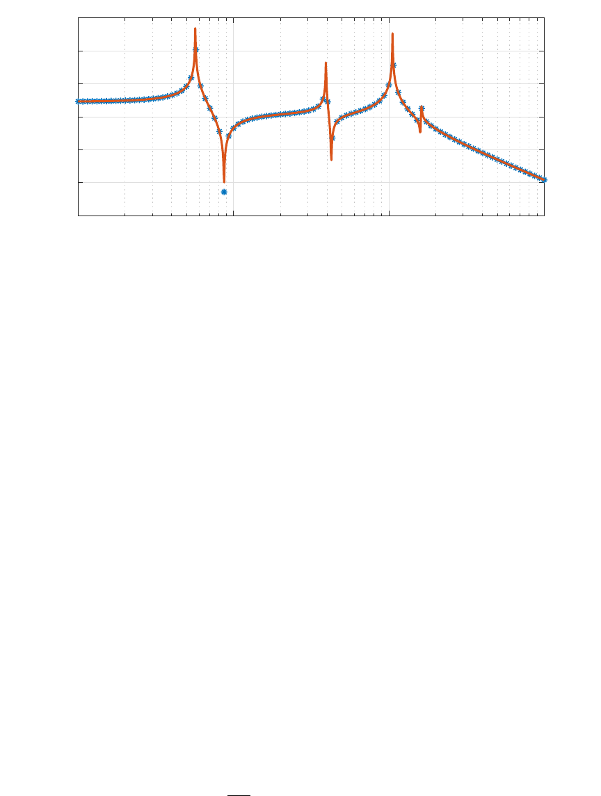
Plot the system’s frequency response function at 100 equally spaced points between 0.1
to 100 rad/sec. Use that plot to estimate the L
2
induced gain of the system. Then use the
preceding bisection algorithm to estimate the induced gain.
The frequency response plotted using MATLAB is shown in Fig. 1. This plots shows points
at 100 sample points between 0.1 and 100 rad/sec (blue asterisks) as well as a more finely
sampled plot with 10, 000 sample points (shown in solid red line). The peak found by the
coarse sampling was 1.0822 (0.3671 dB). So one would estimate the induced gain to be
1.0822. The peak found by the more finely sampled plot was 4.8912 (13.7883 dB). If we
had used the preceding bisection algorithm, we would have found the actual peak to be
8.2664 (18.3463 dB). The induced gain estimated from the gain-magnitude plot depended
greatly on how finely we sampled the plot. The problem here was that we have no way of
relating the sampling interval to the error in our estimate of the induced gain. The bisection
algorithm, on the other hand, does provide a relationship between the number of recursions
and the accuracy of the estimate. In particular, one can guarantee that with an initial guess
between 0 and 10 one would only need 10 recursions to get within 0.01 of the actual gain.
20
10
-1
10
0
10
1
10
2
-100
-80
-60
-40
-20
0
20
FIGURE 1. Sampled Gain magnitude being used to estimate L2 induced
gain
4. L
p
STABILITY AND LYAPUNOV STABILITY
Since Lyapunov stability is such an important concept, it is useful to characterize the rela-
tionship between L
p
stability and Lyapunov stability. This is done in the following theorem
theorem 5. Consider the input-output system ˙x(t) = f(x(t), w(t)) and y(t) = h(x(t), w(t))
where the origin is an exponentially stable equilibrium of ˙x(t) = f(x(t), 0). Assume there
exist positive constants L, r, r
w
, η
1
, and η
2
such that
|f(x, w) − f (x, 0)| ≤ L|w|
|h(x, w)| ≤ η
1
|x| + η
2
|w|
for all |x| < r and |w| < r
w
. If there exists a C
1
function V : R
n
→ R and non-negative
constants c
1
, c
2
, c
3
, and c
4
such that
c
1
|x|
2
≤ V (x) ≤ c
2
|x|
2
˙
V (x, 0) ≤ −c
3
|x|
2
∂V
∂x
≤ c
4
|x|
then the system is finite gain L
p
-stable.

21
Proof: Consider
˙
V along trajectories of the forced system
˙
V =
∂V
∂x
f(x, 0) +
∂V
∂x
[f(x, w) − f (x, 0)]
with the given bounds and the Lipschitz constant, L, for f we get
˙
V ≤ −c
3
|x|
2
+ c
4
L|x||w|
Take W(t) =
p
V (x(t)) and note that
˙
W =
˙
V
2
√
V
We obtain the following differential inequality
˙
W ≤ −
1
2
c
3
c
2
W +
c
4
L
2
√
c
1
|w(t)|
By the comparison principle we can therefore conclude that
W (t) ≤ e
−
c
3
2c
2
t
W (0) +
c
4
L
2
√
c
1
Z
t
0
e
−(t−s)
c
3
2c
2
|w(s)|ds
which implies that
|x(t)| ≤
c
2
c
1
|x
0
|e
−
c
3
2c
2
t
+
c
4
L
2c
1
Z
t
0
e
−(t−s)
c
3
2c
2
|w(s)|ds
and so we can conclude that if |x
0
| ≤
r
2
r
c
1
c
2
and ∥w∥
L
∞
≤
c
1
c
3
r
2c
2
c
4
L
, then |x(t)| ≤ r for all
time.
This means that the bound on h holds for all time and so
|y(t)| ≤ k
1
e
−at
+ k
2
Z
t
0
e
−a(t−s)
|w(s)|ds + k
3
|w(t)|
where k
1
=
r
c
1
c
2
|x
0
|η
1
, k
2
=
c
4
Lη
1
2c
1
, k
3
= η
2
, and a =
c
3
2c
2
. Assign to each of these terms
in the above equation a signal y
1
, y
2
, and y
3
. If w ∈ L
pe
with ∥w∥
L
∞
sufficiently small
then for any T > 0
∥y
2T
∥
L
p
≤
k
2
a
∥w
T
∥
L
p
, ∥y
3T
∥
L
p
≤ k
3
∥w
T
∥
L
p
, ∥y
1T
∥
L
p
≤ k
1
ρ
where ρ =
(
1 if p = ∞
(1/ap)
1/p
otherwise
. So that since
∥y
T
∥
L
p
≤ ∥y
1T
∥
L
p
+ ∥y
2T
∥
L
p
+ ∥y
3T
∥
L
p

22
we can use the above bounds to conclude
∥y
T
∥
L
p
≤ k
1
ρ +
k
2
a
∥w
T
∥
L
p
+ k
3
∥w
T
∥
L
p
=
k
2
a
+ k
3
∥w
T
∥
L
p
+ k
1
ρ = γ∥w
T
∥
L
p
+ β
which identify the finite gain and bias for this system. ♢
For linear time-invariant systems, since the existence of a Lyapunov function is necessary
and sufficient for asymptotic stability of the state, then it is much easier to see that the
system will be L
p
stable. The converse, however is not true. Let us consider,
˙x(t) = Ax(t) + Bw(t)
y(t) = Cx(t)
If the origin is asymptotically stable, then it is exponentially stable and so there exist K > 0
and γ > 0 such that
e
At
x
0
≤ Ke
−γt
for t ≥ 0. Since the impulse response is Ce
At
Bu(t), it is easy to see that this must be
integrable and so if the state-based system is exponentially stable, it must also be L
p
stable.
The converse may not be true as is seen in the following example. Let us consider the
state-based system,
"
˙x
1
(t)
˙x
2
(t)
#
=
"
−1 0
0 1
#"
x
1
(t)
x
2
(t)
#
+
"
1
0
#
w(t), y(t) =
h
1 0
i
"
x
1
(t)
x
2
(t)
#
This system is clearly unstable since the A matrix has one eigenvalue with a positive real
part. This system however is L
p
stable since its transfer function is
1
s+1
which only has a
single pole on the left hand side of the complex plane. The reason why this system is L
p
stable but not asymptotically stable is because the unstable mode of the state-based system
is not observed at the system’s output. Moreover, it is not influenced by the input either.
State-based models that have this property are said to be uncontrollable and unobservable.
Informally, we define these concepts as follows
• Controllability and Reachability mean that there exists a finite duration input that
can drive the system state to any state in R
n
.
23
• Observability and Constructibility mean that we can deduce the system’s initial
state, x(0), given a finite duration set of inputs and outputs.
The main thing to notice here is that controllability and observability are finite time con-
cepts whereas stability characterizes the system’s behavior over an infinite time interval.
The following week’s lectures provide a detailed discussion on the controllability and ob-
servability of linear dynamical systems.
