
This paper is included in the Proceedings of the
16th USENIX Symposium on Networked Systems
Design and Implementation (NSDI ’19).
February 26–28, 2019 • Boston, MA, USA
ISBN 978-1-931971- 49-2
Open access to the Proceedings of the
16th USENIX Symposium on Networked Systems
Design and Implementation (NSDI ’19)
is sponsored by
Shuffling, Fast and Slow: Scalable Analytics
on Serverless Infrastructure
Qifan Pu, UC Berkeley; Shivaram Venkataraman, University of Wisconsin, Madison;
Ion Stoica, UC Berkeley
https://www.usenix.org/conference/nsdi19/presentation/pu

Shuffling, Fast and Slow: Scalable Analytics on Serverless Infrastructure
Qifan Pu (UC Berkeley), Shivaram Venkataraman (UW Madison), Ion Stoica (UC Berkeley)
Abstract
Serverless computing is poised to fulfill the long-held
promise of transparent elasticity and millisecond-level pric-
ing. To achieve this goal, service providers impose a fine-
grained computational model where every function has a
maximum duration, a fixed amount of memory and no persis-
tent local storage. We observe that the fine-grained elasticity
of serverless is key to achieve high utilization for general
computations such as analytics workloads, but that resource
limits make it challenging to implement such applications as
they need to move large amounts of data between functions
that don’t overlap in time. In this paper, we present Locus,
a serverless analytics system that judiciously combines (1)
cheap but slow storage with (2) fast but expensive storage,
to achieve good performance while remaining cost-efficient.
Locus applies a performance model to guide users in select-
ing the type and the amount of storage to achieve the desired
cost-performance trade-off. We evaluate Locus on a number
of analytics applications including TPC-DS, CloudSort, Big
Data Benchmark and show that Locus can navigate the cost-
performance trade-off, leading to 4⇥-500⇥ performance im-
provements over slow storage-only baseline and reducing re-
source usage by up to 59% while achieving comparable per-
formance with running Apache Spark on a cluster of virtual
machines, and within 2⇥ slower compared to Redshift.
1 Introduction
The past decade has seen the widespread adoption of cloud
computing infrastructure where users launch virtual ma-
chines on demand to deploy services on a provisioned clus-
ter. As cloud computing continues to evolve towards more
elasticity, there is a shift to using serverless computing,
where storage and compute is separated for both resource
provisioning and billing. This trend was started by ser-
vices like Google BigQuery [9], and AWS Glue [22] that
provide cluster-free data warehouse analytics, followed by
services like Amazon Athena[5] that allow users to per-
form interactive queries against a remote object storage with-
out provisioning a compute cluster. While the aforemen-
tioned services mostly focus on providing SQL-like analyt-
ics, to meet the growing demand, all major cloud providers
now offer “general” serverless computing platforms, such as
AWS Lambda, Google Cloud Functions, Azure Functions
and IBM OpenWhisk. In these platforms short-lived user-
defined functions are scheduled and executed in the cloud.
Compared to virtual machines, this model provides more
fine-grained elasticity with sub-second start-up times, so that
workload requirements can be dynamically matched with
continuous scaling.
Fine-grained elasticity in serverless platforms is natu-
rally useful for on-demand applications like creating image
thumbnails [18] or processing streaming events [26]. How-
ever, we observe such elasticity also plays an important role
for data analytics workloads. Consider for example an ad-
hoc data analysis job exemplified by say TPC-DS query
95 [34] (See section 5 for more details). This query con-
sists of eight stages and the amount of input data at each
stage varies from 0.8MB to 66GB. With a cluster of virtual
machines users would need to size the cluster to handle the
largest stage leaving resources idle during other stages. Us-
ing a serverless platform can improve resource utilization as
resources can be immediately released after use.
However, directly using a serverless platform for data an-
alytics workloads could lead to extremely inefficient execu-
tion. For example we find that running the CloudSort bench-
mark [40] with 100TB of data on AWS Lambda, can be up
to 500⇥ slower (Section 2.3) when compared to running on
a cluster of VMs. By breaking down the overheads we find
that the main reason for the slowdown comes from slow data
shuffle between asynchronous function invocations. As the
ephemeral, stateless compute units lack any local storage,
and as direct transfers between functions is not always feasi-
ble
1
, intermediate data between stages needs to be persisted
on shared storage systems like Amazon S3. The character-
istics of the storage medium can have a significant impact
on performance and cost. For example, a shuffle from 1000
map tasks to 1000 reduce tasks leads to 1M data blocks being
created on the storage system. Therefore, throughput limits
of object stores like Amazon S3 can lead to significant slow
downs (Section 2.3).
Our key observation is that in addition to using elas-
tic compute and object storage systems we can also pro-
vision fast memory-based resources in the cloud, such as
in-memory Redis or Memcached clusters. While naively
putting all data in fast storage is cost prohibitive, we can ap-
propriately combine fast, but expensive storage with slower
but cheaper storage, similar to the memory and disk hierar-
chy on a local machine, to achieve the best of both worlds:
approach the performance of a pure in-memory execution at
a significantly lower cost. However, achieving such a sweet
spot is not trivial as it depends on a variety of configuration
parameters, including storage type and size, degree of task
parallelism, and the memory size of each serverless func-
1
Cloud providers typically provide no guarantees on concurrent execu-
tion of workers.
USENIX Association 16th USENIX Symposium on Networked Systems Design and Implementation 193

tion. This is further exacerbated by the various performance
limits imposed in a serverless environment (Section 2.4).
In this paper we propose Locus, a serverless analytics sys-
tem that combines multiple storage types to achieve better
performance and resource efficiency. In Locus, we build a
performance model to aid users in selecting the appropriate
storage mechanism, as well as the amount of fast storage
and parallelism to use for map-reduce like jobs in server-
less environments. Our model captures the performance and
cost metrics of various cloud storage systems and we show
how we can combine different storage systems to construct
hybrid shuffle methods. Using simple micro-benchmarks,
we model the performance variations of storage systems as
other variables like serverless function memory and paral-
lelism change.
We evaluate Locus on a number of analytics applications
including TPC-DS, Daytona CloudSort and the Big Data
Benchmark. We show that using fine-grained elasticity, Lo-
cus can reduce cluster time in terms of total core·seconds
by up to 59% while being close to or beating Spark’s query
completion time by up to 2⇥. We also show that with a small
amount of fast storage, for example, with fast storage just
large enough to hold 5% of total shuffle data, Locus matches
Apache Spark in running time on CloudSort benchmark and
is within 13% of the cost of the winning entry in 2016. While
we find Locus to be 2⇥ slower when compared to Ama-
zon Redshift, Locus is still a preferable choice to Redshift
since it requires no provisioning time (vs. minutes to setup a
Redshift cluster) or knowing an optimal cluster size before-
hand. Finally, we also show that our model is able to accu-
rately predict shuffle performance and cost with an average
error of 15.9% and 14.8%, respectively, which allows Locus
to choose the most appropriate shuffle implementation and
other configuration variables.
In summary, the main contributions of this paper are:
• We study the problem of executing general purpose data
analytics on serverless platforms to exploit fine-grained
elasticity and identify the need for efficient shuffles.
• We show how using a small amount of memory-based
fast storage can lead to significant benefits in perfor-
mance while remaining cost effective.
• To aid users in selecting the appropriate storage mech-
anism, We propose Locus, a performance model that
captures the performance and cost metrics of shuffle op-
erations.
• Using extensive evaluation on TPC-DS, CloudSort and
Big Data Benchmark we show that our performance
model is accurate and can lead to 4⇥-500⇥ perfor-
mance improvements over baseline and up to 59% cost
reduction compared to traditional VM deployments,
and within 2⇥ slower compared to Redshift.
2 Background
We first present a brief overview of serverless computing and
compare it with the traditional VM-based instances. Next we
discuss how analytics queries are implemented on serverless
infrastructure and present some of the challenges in execut-
ing large scale shuffles.
2.1 Serverless Computing: What fits?
Recently, cloud providers and open source projects [25, 32]
have proposed services that execute functions in the cloud
or providing Functions-as-a-Service. As of now, these func-
tions are subject to stringent resource limits. For example,
AWS Lambda currently imposes a 5 minute limit on function
duration and 3GB memory limit. Functions are also assumed
to be stateless and are only allocated 512MB of ephemeral
storage. Similar limits are applied by other providers such
as Google Cloud Functions and Azure Functions. Regard-
less of such limitations, these offerings are popular among
users for two main reasons: ease of deployment and flexi-
ble resource allocation. When deploying a cluster of virtual
machines, users need to choose the instance type, number
of instances, and make sure these instances are shutdown
when the computation finishes. In contrast, serverless of-
ferings have a much simpler deployment model where the
functions are automatically triggered based on events, e.g.,
arrival of new data.
Furthermore, due to their lightweight nature, containers
used for serverless deployment can often be launched within
seconds and thus are easier to scale up or scale down when
compared to VMs. The benefits of elasticity are especially
pronounced for workloads where the number of cores re-
quired varies across time. While this naturally happens for
event-driven workloads for example where say users upload
a photo to a service that needs to be compressed and stored,
we find that elasticity is also important for data analytics
workloads. In particular, user-facing ad-hoc queries or ex-
ploratory analytics workloads are often unpredictable yet
have more stringent responsiveness requirements, making it
more difficult to provision a traditional cluster compared to
recurring production workloads.
We present two common scenarios that highlight the im-
portance of elasticitiy. First, consider a stage of tasks being
run as a part of an analytics workload. As most frameworks
use a BSP model [15, 44] the stage completes only when
the last task completes. As the same VMs are used across
stages, the cores where tasks have finished are idle while the
slowest tasks or stragglers complete [3]. In comparison, with
a serverless model, the cores are immediately relinquished
when a task completes. This shows the importance of elastic-
ity within a stage. Second, elasticity is also important across
stages: if we consider say consider TPC-DS query 95 (details
in 5), the query consists of 8 stages with input data per stage
194 16th USENIX Symposium on Networked Systems Design and Implementation USENIX Association
0
2000
4000
6000
8000
0 500 1000 1500 2000
concurrent requests
time (seconds)
Window
Running
Figure 1: S3 rate limiting in action. We use a TCP-like
additive-increase/multiplicative-decrease (AIMD) algorithm to
probe the number of concurrent requests S3 can support for
reading 10KB objects. We see that S3 not only enforces a rate
ceiling, but also continues to fail requests after the rate is re-
duced for a period of time. The specific rate ceiling can change
over time due to S3’s automatic data-partition scaling.
varying from 0.8Mb to 66Gb. With such a large variance in
data size, being able to adjust the number of cores used at
every stage leads to better utilization compared to traditional
VM model.
2.2 Analytics on serverless: Challenges
To execute analytics queries on a serverless infrastructure we
assume the following system model. A driver process, run-
ning on user’s machine, “compiles” the query into a multi-
stage DAG, and then submits each task to the cloud service
provider. A task is executed as one function invocation by
the serverless infrastructure. Tasks in consecutive stages ex-
change data via a variety of communication primitives, such
as shuffle and broadcast [11]. Each task typically consists of
three phases: read, compute, and write [33]. We next discuss
why the communication between stages i.e., the shuffle stage
presents the biggest challenge.
Input, Output: Similar to existing frameworks, each task
running as a function on a serverless infrastructure reads the
input from a shared storage system, such as S3. However,
unlike existing frameworks, functions are not co-located
with the storage, hence there is no data locality in this model.
Fortunately, as prior work has shown, the bandwidth avail-
able between functions and the shared storage system is com-
parable to the disk bandwidths [1], and thus we typically do
not see any significant performance degradation in this step.
Compute: With serverless computing platforms, each func-
tion invocation is put on a new container with a virtualized
compute core. Regardless of the hardware heterogeneity,
recent works have shown that the almost linear scaling of
serverless compute is ideal for supporting embarrassingly
parallel workloads [16, 18].
Shuffle: The most commonly used communication pattern
to transfer data across stages is the shuffle operation. The
map stage partitions data according to the number of reduc-
ers and each reducer reads the corresponding data partitions
from the all the mappers. Given M mappers and R reduc-
ers we will have M ⇤ R intermediate data partitions. Un-
fortunately, the time and resource limitations imposed by
the serverless infrastructures make the implementation of the
shuffle operation highly challenging.
A direct approach to implementing shuffles would be to
open connections between serverless workers [18] and trans-
fer data directly between them. However, there are two lim-
itations that prevent this approach. First cloud providers do
not provide any guarantees on when functions are executed
and hence the sender and receiver workers might not be ex-
ecuting at the same time. Second, even if the sender and
receiver overlap, given the execution time limit, there might
not be enough time to transfer all the necessary data.
A natural approach to transferring data between ephemeral
workers is to store intermediate data in a persistent storage
system. We illustrate challenges for this approach with a
distributed sorting example.
2.3 Scaling Shuffle: CloudSort Example
The main challenge in executing shuffles in a serverless
environment is handling the large number of intermediate
files being generated. As discussed before, functions have
stringent resource limitations and this effectively limits the
amount of data a function can process in one task. For ex-
ample to sort 100TB, we will need to create a large number
of map partitions, as well as a large number of reduce par-
titions, such that the inputs to the tasks can be less than the
memory footprint of a function. Assuming 1GB partitions,
we have 10
5
partitions on both the map side and the reduce
side. For implementing a hash-based shuffle one intermedi-
ate file is created for each (mapper, reducer) pair. In this case
we will have a total of 10
10
, or 10 billion intermediate files!
Even with traditional cluster-based deployment, shuffling 10
billion files is quite challenging, as it requires careful opti-
mization to achieve high network utilization [31]. Unfortu-
nately, none of the storage systems offered by existing cloud
providers meets the performance requirements, while also
being cost-effective. We next survey two widely available
storage systems classes and discuss their characteristics.
2.4 Cloud Storage Systems Comparison
To support the diverse set of cloud applications, cloud
providers offer a number of storage systems each with dif-
ferent characteristics in terms of latency, throughput, stor-
age capacity and elasticity. Just as within a single machine,
where we have a storage hierarchy of cache, memory and
disk, each with different performance and cost points, we
observe that a similar hierarchy can be applied to cloud stor-
age systems. We next categorize two major storage system
classes.
Slow Storage: All the popular cloud providers offer sup-
port for scalable and elastic blob storage. Examples of such
USENIX Association 16th USENIX Symposium on Networked Systems Design and Implementation 195
systems include Amazon S3, Google Cloud Storage, Azure
Blob Store. However, these storage systems are not designed
to support high throughput on reading and writing small files.
In fact, all major public cloud providers impose a global
transaction limit on shared object stores [37, 7, 20]. This
should come as no surprise, as starting with the Google File
System [21], the majority of large scale storage systems have
been optimized for reading and writing large chunks of data,
rather than for high-throughput fine-grained operations.
We investigated the maximum throughput that one can
achieve on Amazon S3 and found that though the through-
put can be improved as the number of buckets increases,
the cloud provider throttles requests when the aggregate
throughput reaches a few thousands of requests/sec (see Fig-
ure 1). Assuming a throughput of 10K operations per second,
this means that reading and writing all the files generated
by our CloudSort example could take around 2M seconds,
or 500⇥ slower than the current record [42]. Not only is
the performance very low, but the cost is prohibitive as well.
While the cost per write request is as low as $0.005 per 1,000
requests for all three aforementioned cloud providers, shuf-
fling 10
10
files would cost $5,000 alone for write requests.
Thus, supporting large shuffles requires a more efficient and
economic solution for storing intermediate data.
Fast Storage: One approach to overcome the performance
limitations of the slow storage systems is to use much faster
storage, if available. Examples of faster storage are in-
memory storage systems backed by Memcached or Redis.
Such storage systems support much higher request rates
(more than 100,000 requests/sec per shard), and efficiently
handle objects as small as a few tens of bytes. On the flip
side, these systems are typically much more expensive than
large-scale blob storage systems. For example to store 1GB
of data for an hour, it costs 0.00319 cents in AWS S3 while it
costs 2.344 cents if we use a managed Redis service such as
AWS ElastiCache, which makes it 733⇥ more expensive!
2
Given the cost-performance trade-off between slow (e.g.,
S3) and fast (e.g., ElastiCache) storage, in the following
sections we show that by judiciously combining these two
types of storage systems, we can achieve a cost-performance
sweet spot in a serverless deployment that is comparable, and
sometimes superior to cluster-based deployments.
3 Design
In this section we outline a performance model that can be
used to guide the design of an efficient and cost-effective
shuffle operations. We start with outlining our system model,
2
We note that ElastiCache is not “serverless”, and there is no server-
less cache service yet as of writing this paper and users need to provision
cache instances. However, we envision that similar to existing storage and
compute, fast storage as a resource (possibly backed by memory) will also
become elastic in the future. There are already several proposals to provide
disaggregated memory across datacenters [19] to support this.
0
20
40
60
80
100
0.5G 1G 1.5G 2G 3G
write BW/worker (MB/sec)
1
10
300
1000
3000
(a) write
0
20
40
60
80
100
0.5G 1G 1.5G 2G 3G
read BW/worker (MB/sec)
1
10
300
1000
3000
(b) read
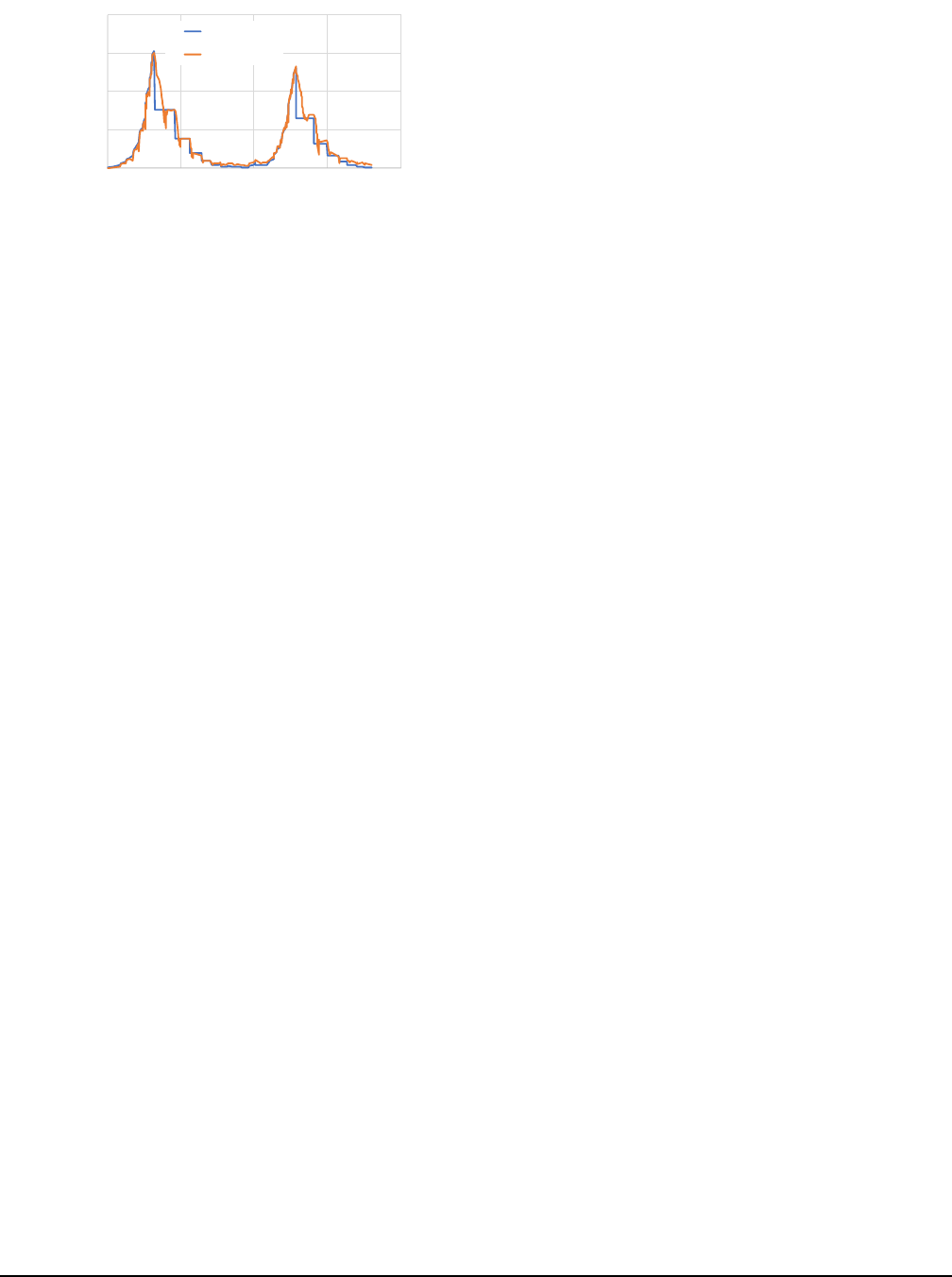
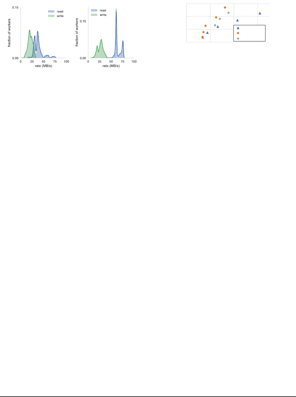
Figure 2: S3 bandwidth per worker with varying concur-
rency (1 to 3000) and Lambda worker size (0.5G to 3G).
Table 1: Measured throughput (requests/sec) limit for a single
S3 bucket and a single Redis shard.
object size 10KB 100KB 1M 10M 100M
S3 5986 4400 3210 1729 1105
Redis 116181 11923 1201 120 12
and then discuss how different variables like worker memory
size, degree of parallelism, and the type of storage system af-
fect the performance characteristics of the shuffle operation.
3.1 System Model
We first develop a high level system model that can be used
to compare different approaches to shuffle and abstract away
details specific to cloud providers. We denote the function-
as-a-service module as compute cores or workers for tasks.
Each function invocation, or a worker, is denoted to run with
a single core and w bytes of memory (or the worker memory
size). The degree of the parallelism represents the number
of function invocations or workers that execute in parallel,
which we denote by p. The total amount of data being shuf-
fled is S bytes. Thus, the number of workers required in the
map and reduce phase is at least
S
w
leading to a total of (
S
w
)
2
requests for a full shuffle.
We next denote the bandwidth available to access a storage
service by an individual worker as b bytes/sec. We assume
that the bandwidth provided by the elastic storage services
scale as we add more workers (we discuss how to handle
cases where this is not true below). Finally, we assume each
storage service limits the aggregate number of requests/sec:
we denote by q
s
and q
f
for the slow and the fast storage
systems, respectively.
To measure the cost of each approach we denote the cost
of a worker function as c
l
$/sec/byte, the cost of fast storage
as c
f
$/sec/byte. The cost of slow storage has two parts, one
for storage as c
s
$/sec/byte, and one for access, denoted as c
a
$/op. We assume that both the inputs and the outputs of the
shuffle are stored on the slow storage. In most cases in prac-
tice, c
s
is negligible during execution of a job. We find the
196 16th USENIX Symposium on Networked Systems Design and Implementation USENIX Association
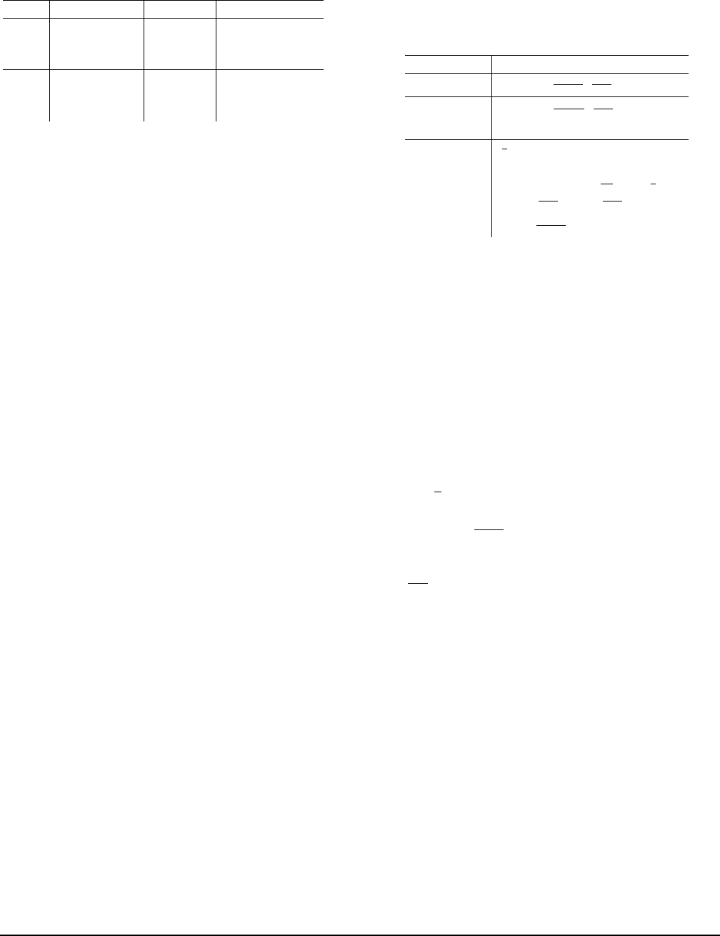
Table 2: Cloud storage cost from major providers (Feb 2019).
Service $/Mo/GB $/million writes
Slow
AWS S3 0.023 5
GCS 0.026 5
Azure Blob 0.023 6.25
Fast
ElastiCache 7.9 -
Memorystore 16.5 -
Azure Cache 11.6 -
above cost characteristics apply to all major cloud platforms
(AWS, Google Cloud and Azure), as shown in Table 2.
Among the above, we assume the shuffle size (S) is given
as an input to the model, while the worker memory size (w),
the degree of parallelism (p), and the amount of fast storage
(r) are the model knobs we vary. To determine the character-
istics of the storage systems (e.g., b, q
s
, q
f
), we use offline
benchmarking. We first discuss how these storage perfor-
mance characteristics vary as a function of our variables.
3.2 Storage Characteristics
The main storage characteristics that affect performance are
unsurprisingly the read and write throughput (in terms of
requests/sec, or often referred as IOPS) and bandwidth (in
terms of bytes/sec). However, we find that these values are
not stable as we change the degree of parallelism and worker
memory size. In Figure 2 we measure how a function’s band-
width (b) to a large-scale store (i.e., Amazon S3, the slow
storage service in our case) varies as we change the degree
of parallelism (p) and the worker memory size (w). From
the figure we can see that as we increase the parallelism both
read and write bandwidths could vary by 2-3⇥. Further we
see that as we increase the worker memory size the band-
width available increases but that the increase is sub-linear.
For example with 60 workers each having 0.5G of memory,
the write bandwidth is around 18 MB/s per worker or 1080
MB/s in aggregate. If we instead use 10 workers each hav-
ing 3GB of memory, the write bandwidth is only around 40
MB/s per worker leading to 400 MB/s in aggregate.
Using a large number of small workers is not always ideal
as it could lead to an increase in the number of small I/O re-
quests. Table 1 shows the throughput we get as we vary the
object size. As expected, we see that using smaller object
sizes means that we get a lower aggregate bandwidth (mul-
tiplying object size by transaction throughput). Thus, jointly
managing worker memory size and parallelism poses a chal-
lenging trade-off.
For fast storage systems we typically find that through-
put is not a bottleneck for object sizes > 10 KB and that we
saturate the storage bandwidth. Hence, as shown in Table 1
the operation throughput decreases linearly as the object size
increases. While we can estimate the bandwidth available
for fast storage systems using an approach similar to the
one used for slow storage systems, the current deployment
Table 3: Comparison of time taken by different shuffle meth-
ods. S refers to the shuffle data size, w to the worker memory
size, p the number of workers, q
s
the throughput to slow stor-
age, q
f
throughput to fast storage b network bandwidth from
each worker.
storage type shuffle time
slow 2 ⇥ max(
S
2
w
2
⇥q
s
,
S
b⇥p
)
fast 2 ⇥ max(
S
2
w
2
⇥q
f
,
S
b
ef f
), where
b
ef f
= min(b
f
,b ⇥ p)
hybrid
S
r
T
rnd
+ T
mrg
, where
T
rnd
= 2 ⇥ max(T
fb
,T
sb
,T
sq
)
T
mrg
= 2 ⇥ max((
Sw
r
)
2
T
sq
,
S
r
T
sb
)
T
fb
=
r
b
ef f
, T
sb
=
r
b⇥p
T
sq
=
r
2
w
2
⇥q
s
method where we are allocating servers for running Mem-
cached / Redis allows us to ensure they are not a bottleneck.
3.3 Shuffle Cost Models
We next outline performance models for three shuffle sce-
narios: using (1) slow storage only, (2) fast storage only, and
(3) a combination of fast and slow storage.
Slow storage based shuffle. The first model we develop is
using slow storage only to perform the shuffle operation. As
we discussed in the previous section there are two limits that
the slow storage systems impose: an operation throughput
limit (q
s
) and a bandwidth limit (b). Given that we need to
perform (
S
w
)
2
requests with an overall operation throughput
of q
s
, we can derive T
q
, the time it takes to complete these
requests is T
q
=
S
2
w
2
⇥q
s
, assuming q
s
is the bottleneck. Sim-
ilarly, given the per-worker bandwidth limit to storage, b,
the time to complete all requests assuming b is bottleneck is
T
b
=
S
b⇥p
. Considering both potential bottlenecks, the time it
takes to write/read all the data to/from intermediate storage is
thus max(T
q
,T
b
). Note that this time already includes read-
ing data from input storage or writing data to output storage,
since they can be pipelined with reading/writing to interme-
diate storage. Finally, the shuffle needs to first write data to
storage and then read it back. Hence the total shuffle time is
T
shu f
= 2 ⇥ max(T
q
,T
b
).
Table 4 shows our estimated running time and cost as we
vary the worker memory and data size.
Fast storage based-shuffle. Here we develop a simple
performance model for fast storage that incorporates the
throughput and bandwidth limits. In practice we need
to make one modification to factor in today’s deployment
model for fast storage systems. Since services like Elasti-
Cache are deployed by choosing a fixed number of instances,
each having some fixed amount of memory, the aggregate
bandwidth of the fast storage system could be a significant
bottleneck, if we are not careful. For example, if we had
USENIX Association 16th USENIX Symposium on Networked Systems Design and Implementation 197
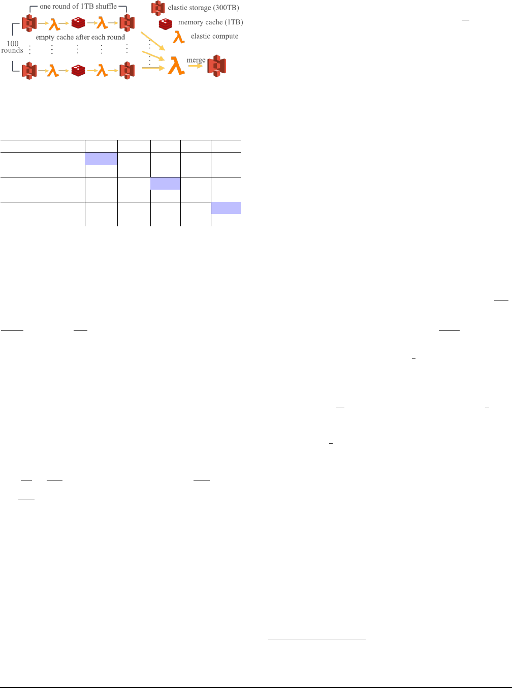
Figure 3: Illustration for hybrid shuffle.
Table 4: Projected sort time and cost with varying worker
memory size. Smaller worker memory results in higher par-
allelism, but also a larger numbers files to shuffle.
worker mem(GB) 0.25 0.5 1 1.25 1.5
20GB time(s) 36 45 50 63 72
20GB cost($) 0.02 0.03 0.03 0.04 0.05
200GB time(s) 305 92 50 63 75
200GB cost($) 0.24 0.30 0.33 0.42 0.51
1TB time(s) 6368 1859 558 382 281
1TB cost($) 1.22 1.58 1.70 2.12 2.54
just one ElastiCache instance with 10Gbps NIC and 50G
of memory, the aggregate bandwidth is trivially limited to
10Gbps. In order to model this aspect, we extend our for-
mulation to include b
f
, which is the server-side bandwidth
limit for fast storage. We calculate the effective bandwidth
as b
ef f
= min(b ⇥ p, b
f
).
Using the above effective bandwidth we can derive the
time taken due to throughput and bandwidth limits as T
q
=
S
2
w
2
⇥q
f
and T
b
=
S
b
ef f
, respectively. Similar to the previ-
ous scenario, the total shuffle time is then T
shu f
= 2 ⇥
max(T
q
,T
b
).
One interesting scenario in this case is that as long as the
fast storage bandwidth is a bottleneck (i.e. b
f
< b ⇥ p), using
more fast memory improves not only the performance, but
also reduces the cost! Assume the amount of fast storage is
r. This translates to a cost of p ⇤ c
l
⇤ T
shu f
+ r ⇤ c
f
⇤ T
shu f
,
with slow storage request cost excluded. Now, assume we
double the memory capacity to 2⇥r, which will also result in
doubling the bandwidth, i.e., 2⇥b
f
. Assuming that operation
throughput is not the bottleneck, the shuffle operations takes
now
S
2b
f
=
T
shu f
2
, while the cost becomes p ⇤ c
l
⇤
T
shu f
2
+2⇤r ⇤
c
f
⇤
T
shu f
2
. This does not include reduction in request cost for
slow storage. Thus, while the cost for fast storage (second
term) remains constant, the cost for compute cores drops by
a factor of 2. In other words, the overall running time has
improved by a factor of 2 while the cost has decreased.
However, as the amount of shuffle data grows, the cost
of storing all the intermediate data in fast storage becomes
prohibitive. We next look at the design of a hybrid shuffle
method that can scale to much larger data sizes.
3.4 Hybrid Shuffle
We propose a hybrid shuffle method that combines the inex-
pensive slow storage with the high throughput of fast storage
to reach a better cost-performance trade-off. We find that
even with a small fast storage, e.g., less than
1
20
th of total
shuffle data, our hybrid shuffle can outperform slow storage
based shuffle by orders of magnitude.
To do that, we introduce a multi-round shuffle that uses
fast storage for intermediate data within a round, and uses
slow storage to merge intermediate data across rounds. In
each round we range-partition the data into a number of
buckets in fast storage and then combine the partitioned
ranges using the slow storage. We reuse the same range par-
titioner across rounds. In this way, we can use a merge stage
at the end to combine results across all rounds, as illustrated
in Figure 3. For example, a 100 TB sort can be broken down
to 100 rounds of 1TB sort, or 10 rounds of 10TB sort.
Correspondingly the cost model for the hybrid shuffle can
be broken down into two parts: the cost per round and the
cost for the merge. The size of each round is fixed at r, the
amount of space available on fast storage. In each round we
perform two stages of computation, partition and combine.
In the partition stage, we read input data from the slow stor-
age and write to the fast storage, while in the combine stage
we read from the fast storage and write to the slow storage.
The time taken by one stage is then the maximum between
the corresponding durations of the stage when the bottleneck
is driven either by (1) the fast storage bandwidth T
fb
=
r
b
ef f
,
(2) the slow storage bandwidth T
sb
= r/(b ⇤ p), or (3) the
slow storage operation throughput T
sq
=
r
2
w
2
⇥q
s
3
. Thus, the
time per-round is T
rnd
= 2 ⇤ max(T
fb
,T
sb
,T
sq
).
The overall shuffle consists of
S
r
such rounds and a fi-
nal merge phase where we read data from the slow storage,
merge it, and write it back to the slow storage. The time of
the merge phase can be similarly broken down into through-
put limit T
mq
=(
Sw
r
)
2
⇤ T
sq
and bandwidth limit T
mb
=
S
r
⇤ T
sb
,
where T
sb
and T
sq
follows from the definitions from previ-
ous paragraph. Thus, T
mrg
= 2 ⇤ max(T
mq
,T
mb
), and the total
shuffle time is
S
r
⇤ T
rnd
+ T
mrg
.
How to pick the right fast storage size? Selecting the
appropriate fast storage/memory size is crucial to obtaining
good performance with the hybrid shuffle. Our performance
model aims to determine the optimal memory size by using
two limits to guide the search. First, provisioning fast storage
does not help when slow storage bandwidth becomes bottle-
neck, which provides an upper bound on fast storage size.
Second, since the final stage needs to read outputs from all
prior rounds to perform the merge, the operation throughput
of the slow storage provides an upper bound on the number
of rounds, thus a lower bound of the fast storage size.
Pipelining across stages An additional optimization we per-
form to speed up round execution and reduce cost is to
pipeline across partition stage and combine stage. As shown
in Figure 3, for each round, we launch partition tasks to read
3
We ignore the fast storage throughput, as we rarely find it to be bottle-
neck. We could easily include it in our model, if needed.
198 16th USENIX Symposium on Networked Systems Design and Implementation USENIX Association
(a) 500MB workers (b) 3GB workers
Figure 4: Lambda to S3 bandwidth distribution exhibits
high variance. A major source of stragglers.
input data, partition them and write out intermediate files to
the fast storage. Next, we launch combine tasks that read
files from the fast storage. After each round, the fast storage
can be cleared to be used for next round.
With pipelining, we can have partition tasks and combine
tasks running in parallel. While the partition tasks are writ-
ing to fast storage via append(), the merge tasks read out
files periodically and perform atomic delete-after-read op-
erations to free space. Most modern key-value stores, e.g.,
Redis, support operations such as append and atomic delete-
after-read. Pipelining gives two benefits: (1) it overlaps the
execution of the two phases thus speeding up the in-round
sort, and (2) it allows a larger round size without needing
to store the entire round in memory. Pipelining does have a
drawback. Since we now remove synchronization boundary
between rounds, and use append() instead of setting a new
key for each intermediate data, we cannot apply speculative
execution to mitigate stragglers, nor can we obtain task-level
fault tolerance. Therefore, pipelining is more suitable for
smaller shuffles.
3.5 Modeling Stragglers
The prior sections provided several basic models to estimate
the time taken by a shuffle operation in a serverless environ-
ment. However, these basic models assume all tasks have
uniform performance, thus failing to account for the pres-
ence of stragglers.
The main source of stragglers for the shuffle tasks we con-
sider in this paper are network stragglers, that are caused by
slow I/O to object store. Network stragglers are inherent
given the aggressive storage sharing implied by the server-
less architecture. While some containers (workers) might get
better bandwidth than running reserved instances, some con-
tainers get between 4-8⇥ lower bandwidth, as shown in Fig-
ure 4. To model the straggler mitigation scheme described
above we initialize our model with the network bandwidth
CDFs as shown in Figure 4. To determine running time of
each stage we then use an execution simulator [33] and sam-
ple network bandwidths for each container from the CDFs.
20GB
100GB
1TB
10TB
100TB
0.01
1
100
10000
1 100 10000 1000000
predicted cost ($)
predicted sh uffle time (seconds)
slow;storage
fast;storage
hybrid; (>1TB)
Figure 5: Predicted time and cost for different sort implemen-
tations and sizes.
Furthermore, our modeling is done for each worker memory
size, since bandwidth CDFs vary across worker sizes.
There are many previous works on straggler mitiga-
tion [45, 4, 36, 2]. We use a simple online method where
we always launch speculative copies after x% of tasks finish
in the last wave. Having short-lived tasks in the serverless
model is more advantageous here. The natural elasticity of
serverless infrastructure makes it possible to be aggressive in
launching speculative copies.
3.6 Performance Model Case Study
We next apply our performance model described above to the
CloudSort benchmark and study the cost-performance trade-
off for the three approaches described above. Our predic-
tions for data sizes ranging from 20GB to 100TB are shown
in Figure 5 (we use experimental results of a real prototype
to validate these predictions in Section 5). When the data
shuffle size is small (e.g., 20GB or smaller), both the slow
and fast storage only solutions take roughly the same time,
with the slow storage being slightly cheaper. As the data size
increases to around 100GB, using fast storage is around 2⇥
faster for the same cost. This speed up from fast storage is
more pronounced as data size grows. For very large shuffles
( 10 TB), hybrid shuffle can provide significant cost sav-
ings. For example, at 100TB, the hybrid shuffle is around 6x
cheaper than the fast storage only shuffle, but only 2x slower.
Note that since the hybrid shuffle performs a merge phase
in addition to writing all the data to the fast storage, it is al-
ways slower than the fast storage only shuffle. In summary,
this example shows how our performance model can be used
to understand the cost-performance trade-off from using dif-
ferent shuffle implementations. We implement this perfor-
mance modeling framework in Locus to perform automatic
shuffle optimization. We next describe the implementation
of Locus and discuss some extensions to our model.
4 Implementation
We implement Locus by extending PyWren [16], a Python-
based data analytics engine developed for serverless envi-
ronments. PyWren allows users to implement custom func-
tions that perform data shuffles with other cloud services,
but it lacks an actual shuffle operator. We augment PyWren
USENIX Association 16th USENIX Symposium on Networked Systems Design and Implementation 199

with support for shuffle operations and implement the per-
formance modeling framework described before to automat-
ically configure the shuffle variables. For our implementa-
tion we use AWS Lambda as our compute engine and use
S3 as the slow, elastic storage system. For fast storage we
provision Redis nodes on Amazon ElastiCache.
To execute SQL queries on Locus, we devise physical
query plan from Apache Spark and then use Pandas to imple-
ment structured data operations. One downside with Pandas
is that we cannot do “fine-grained pipelining” between data
operations inside a task. Whereas in Apache Spark or Red-
shift, a task can process records as they are read in or writ-
ten out. Note this fine-grained pipelining is different from
pipelining across stages, which we discuss in Section 3.4.
4.1 Model extensions
We next discuss a number of extensions to augment the per-
formance model described in the previous section
Non-uniform data access: The shuffle scenario we con-
sidered in the previous section was the most general all-to-
all shuffle scenario where every mapper contributes data to
every reducer. However, a number of big data workloads
have more skewed data access patterns. For example, ma-
chine learning workloads typically perform AllReduce or
broadcast operations that are implemented using a tree-
based communication topology. When a binary tree is used
to do AllReduce, each mapper only produces data for one re-
ducer and correspondingly each reducer only reads two parti-
tions. Similarly while executing a broadcast join, the smaller
table will be accessed by every reducer while the larger ta-
ble is hash partitioned. Thus, in these scenarios storing the
more frequently accessed partition on fast storage will im-
prove performance. To handle these scenarios we introduce
an access counter for each shuffle partition and correspond-
ingly update the performance model. We only support this
currently for cases like AllReduce and broadcast join where
the access pattern is known beforehand.
Storage benchmark updates: Finally one of the key factors
that make our performance models accurate is the storage
benchmarks that measure throughput (operations per sec)
and network bandwidth (bytes per second) of each storage
system. We envision that we will execute these benchmarks
the first time a user installs Locus and that the benchmark
values are reused across a number of queries. However, since
the benchmarks are capturing the behavior of cloud storage
systems, the performance characteristics could change over
time. Such limits change will require Locus to rerun the pro-
filing. We plan to investigate techniques where we can pro-
file query execution to infer whether our benchmarks are still
accurate over extended periods of time.
5 Evaluation
We evaluate Locus with a number of analytics workloads,
and compare Locus with Apache Spark running on a cluster
of VMs and AWS Redshift/Redshift Spectrum
4
. Our evalu-
ation shows that:
• Locus’s serverless model can reduce cluster time by up
to 59%, and at the same time being close to or beating
Spark’s query completion time by up to 2⇥. Even with
a small amount of fast storage, Locus can greatly im-
prove performance. For example, with just 5% memory,
we match Spark in running time on CloudSort bench-
mark and are within 13% of the cost of the winning
entry in 2016.
• When comparing with actual experiment results, our
model in Section 3 is able to predict shuffle perfor-
mance and cost accurately, with an average error of
15.9% for performance and 14.8% for cost. This allows
Locus to choose the best cost-effective shuffle imple-
mentation and configuration.
• When running data intensive queries on the same num-
ber of cores, Locus is within 1.61 ⇥ slower compared
to Spark, and within 2 ⇥ slower compared to Redshift,
regardless of the baselines’ more expensive unit-time
pricing. Compared to shuffling only through slow stor-
age, Locus can be up to 4⇥-500⇥ faster.
The section is organized as follows, we first show uti-
lization and end-to-end performance with Locus on TPC-
DS [34] queries ( 5.1) and Daytona CloudSort benchmark
( 5.2). We then discuss how fast storage shifts resource bal-
ance to affect the cost-performance trade-off in Section 5.3.
Using the sort benchmark, we also check whether our shuf-
fle formulation in Section 3 can accurately predict cost and
performance( 5.4). Finally we evaluate Locus’s performance
on joins with Big Data Benchmark [8]( 5.5).
Setup: We run our experiments on AWS Lambda and use
Amazon S3 for slow storage. For fast storage, we use a clus-
ter of r4.2xlarge instances (61GB memory, up to 10Gbps
network) and run Redis. For our comparisons against Spark,
we use the latest version of Apache Spark (2.3.1). For com-
parison against Redshift, we use the latest version as of 2018
September and ds2.8xlarge instances. To calculate cost
for VM-based experiments we pro-rate the hourly cost to a
second granularity.
5
For Redshift, the cost is two parts using
AWS pricing model, calculated by the uptime cost of cluster
VMs, plus $5 per TB data scanned.
4
When reading data of S3, AWS Redshift automatically uses a shared,
serverless pool of resource called the Spectrum layer for S3 I/O, ETL and
partial aggregation.
5
This is presenting a lower cost than the minute-granularity used for
billing by cloud providers like Amazon, Google.
200 16th USENIX Symposium on Networked Systems Design and Implementation USENIX Association
0
50000
100000
150000
200000
250000
Q1 Q16 Q94 Q95
cluster time (core·sec)
Locus
Spark
Redshift
+1%
-58%
-59%
-4%
(a) Cluster time
159
0
100
200
300
400
500
Q1 Q16 Q94 Q95
average query time (s)
Locus-S3
Locus-reserved
Locus
Spark
Redshift
(b) Query latency
0
0.5
1
1.5
2
2.5
3
3.5
Q1 Q16 Q94 Q95
cost ($)
Locus
Spark
Redshift
(c) Cost
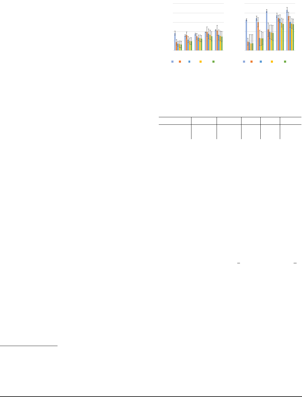
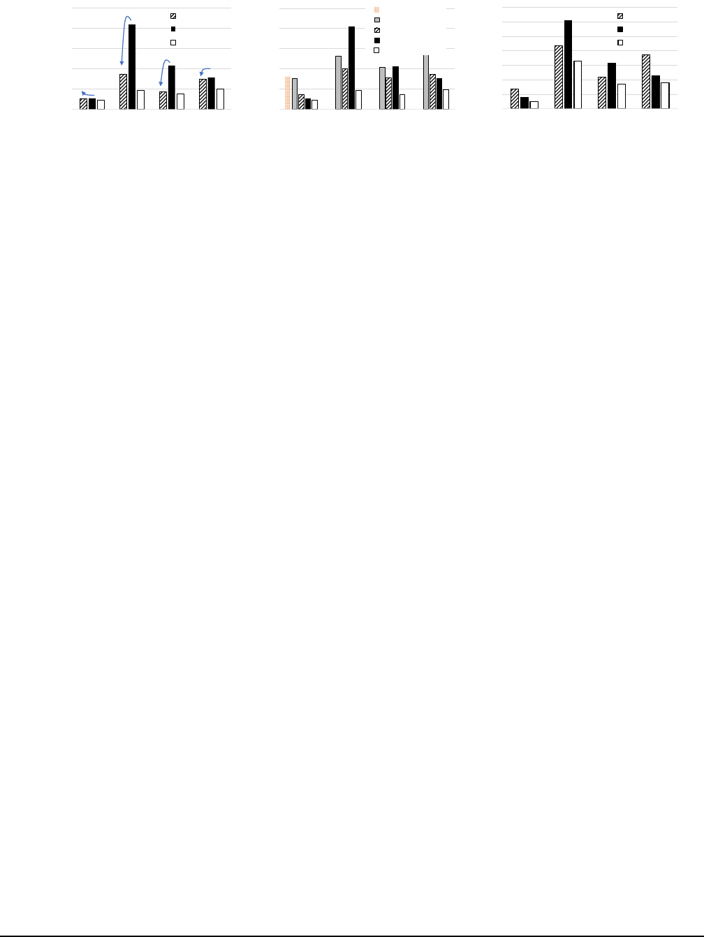
Figure 6: TPC-DS results for Locus, Apache Spark and Redshift under different configurations. Locus-S3 runs the
benchmark with only S3 and doesn’t complete for many queries; Locus-reserved runs Locus on a cluster of VMs.
5.1 TPC-DS Queries
The TPC-DS benchmark has a set of standard decision sup-
port queries based on those used by retail product suppli-
ers. The queries vary in terms of compute and network I/O
loads. We evaluate Locus on TPC-DS with scale factor of
1000, which has a total input size of 1TB data for various ta-
bles. Among all queries, we pick four of them that represent
different performance characteristics and have a varying in-
put data size from 33GB to 312GB. Our baselines are Spark
SQL deployed on a EC2 cluster with c3.8xlarge instances
and Redshift with ds2.8xlarge instances, both with 512
cores. For Locus, we obtain workers dynamically across dif-
ferent stages of a query, but make sure that we never use
more core·secs of Spark execution.
Figure 6(b) shows the query completion time for running
TPC-DS queries on Apache Spark, Redshift and Locus un-
der different configurations and Figure 6(a) shows the the
total core·secs spent on running those queries. We see that
Locus can save cluster time up to 59%, while being close
to Spark’s query completion time to also beating it by 2⇥.
Locus loses to Spark on Q1 by 20s. As a result, even for
now AWS Lambda’s unit time cost per core is 1.92⇥ more
expensive than the EC2 c3.8xlarge instances, Locus en-
joys a lower cost for Q1 and Q4 as we only allocate as many
Lambdas as needed. Compared to Redshift, Locus is 1.56⇥
to 1.99⇥ slower. There are several causes that might con-
tribute to the cost-performance gap: 1) Redshift has a more
efficient execution workflow than that of Locus, which is
implemented in Python and has no fine-grained pipelining;
2) ds2.8xlarge are special instances that have 25Gbps ag-
gregate network bandwidths; 3) When processing S3 data,
AWS Redshift pools extra resource, referred as the serverless
Spectrum layer, to process S3 I/O, ETL and partial aggrega-
tion. To validate these hypotheses, we perform two what-if
analyses. We first take Locus’s TPC-DS execution trace and
replay them to numerically simulate an pipelined execution
by overlapping I/O and compute within a task. We find that
with pipelining, query latencies can be reduced by 23% to
37%, being much closer to the Redshift numbers. Similarly,
using our cost-performance model, we also find that if Lo-
cus’s Redis nodes have 25Gbps links, the cost can be further
reduced by 19%, due to a smaller number of nodes needed.
Performance will not improve due to 25Gbps links, as net-
work bottleneck on Lambda-side remains. Understanding re-
maining performance gap would require further breakdown,
i.e., porting Locus to a lower-level programming language.
Even with the performance gap, an user may still prefer
Locus over a data warehousing service like Redshift since
the latter requires on-demand provisioning of a cluster. Cur-
rently with Amazon Redshift, provisioning a cluster takes
minutes to finish, which is longer than these TPC-DS query
latencies. Picking an optimal cluster size for a query is also
difficult without knowledge of underlying data.
We also see in Figure 6(b) that Locus provides better per-
formance than running on a cluster of 512-core VMs (Locus-
reserved). This demonstrates the power of elasticity in exe-
cuting analytics queries. Finally, using the fast storage based
shuffle in Locus also results in successful execution of 3
queries that could not be executed with slow storage based
shuffle, as the case for Locus-S3 or PyWren.
To understand where time is spent, we breakdown exe-
cution time into different stages and resources for Q94, as
shown in Figure 7. We see that performing compute and
network I/O takes up most of the query time. One way to
improve overall performance given this breakdown is to do
“fine-grained pipelining” of compute and network inside a
task. Though nothing fundamental, it is unfortunately diffi-
cult to implement with the constraints of Pandas API at the
time of writing. Compute time can also be improved if Locus
is prototyped using a lower-level language such as C++.
Finally, for shuffle intensive stages such as stage 3 of Q94,
we see that linearly scaling up fast storage does linearly im-
prove shuffle performance (Figure 8).
5.2 CloudSort Benchmark
We run the Daytona CloudSort benchmark to compare Locus
against both Spark and Redshift on reserved VMs.
The winner entry of CloudSort benchmark which ranks
the cost for sorting 100TB data on public cloud is currently
held by Apache Spark [42]. The record for sorting 100TB
USENIX Association 16th USENIX Symposium on Networked Systems Design and Implementation 201
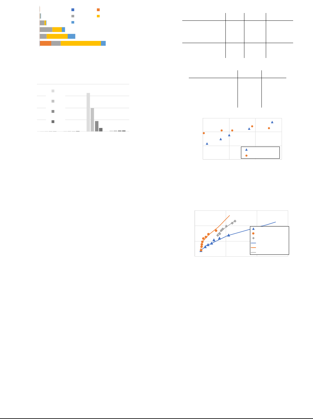
49
27
19
5
1
1
0 20 40 60
1
2
3
4
5
6
time (s)
stage index
start setup
read compute
write total
Figure 7: Time breakdown for Q94. Each stage has a different
profile and, compute and network time dominate.
0
20
40
60
80
start
setup
network
compute
average time (s)
2
4
8
10
Figure 8: Runtime for stage 3 of Q94 when varying the number
of Redis nodes (2, 4, 8, 10).
was achieved in 2983.33s using a cluster of 395 VMs, each
with 4 vCPU cores and 8GB memory. The cost of run-
ning this was reported as $144.22. To obtain Spark num-
bers for 1TB and 10TB sort sizes, we varied the number of
i2.8xlarge instances until the sort times matched those ob-
tained by Locus. This allows a fair comparison on the cost.
As discussed in Section 3, Locus automatically picks the best
shuffle implementation for each input size.
Table 5 shows the result cost and performance compar-
ing Locus against Spark. We see that regardless of the fact
Locus’s sort runs on memory-constrained compute infras-
tructure and communicates through remote storage, we are
within 13% of the cost for 100TB record, and achieve the
same performance. Locus is even cheaper for 10TB (by
15%) but is 73% more expensive for 1TB. This is due to
using fast storage based-shuffle which yields a more costly
trade-off point. We discuss more trade-offs in Section 5.3.
Table 6 shows the result of sorting 1TB of random string
input. Since Redshift does not support querying against ran-
dom binary data, we instead generate random string records
as the sort input as an approximation to the Daytona Cloud-
Sort benchmark. For fair comparison, we also run other sys-
tems with the same string dataset. We see that Locus is an or-
der of magnitude faster than Spark and Redshift and is com-
parable to Spark when input is stored on local disk.
We also run the same Locus code on EC2 VMs, in order
to see the cost vs. performance difference of only chang-
ing hardware infrastructure while using the same program-
ming language (Python in Locus). Figure 9 shows the results
for running 100GB sort. We run Locus on AWS Lambda
with various worker memory sizes. Similar to previous sec-
tion, we then run Locus on a cluster and vary the number
Table 5: CloudSort results vs. Apache Spark
Sort size 1TB 10TB 100TB
Spark nodes 21 60 395[31]
Spark time (s) 40 394 2983
Locus time (s) 39 379 2945
Spark cost ($) 1.5 34 144
Locus cost ($) 2.6 29 163
Table 6: 1TB string sort w/ various configurations
time cost($)
Redshift-S3 6m8s 20.2
Spark RDD-S3 4m27s 15.7
Spark-HDFS ($) 35s 2.1
Locus ($) 39s 2.6
27
24 22
20
17
0.5
1
1.5
2
3
0.1
0.2
0.3
0.4
75 100 125 150
cost ($)
shuffle time (seconds)
Locus-serverl ess
Locus-reserved
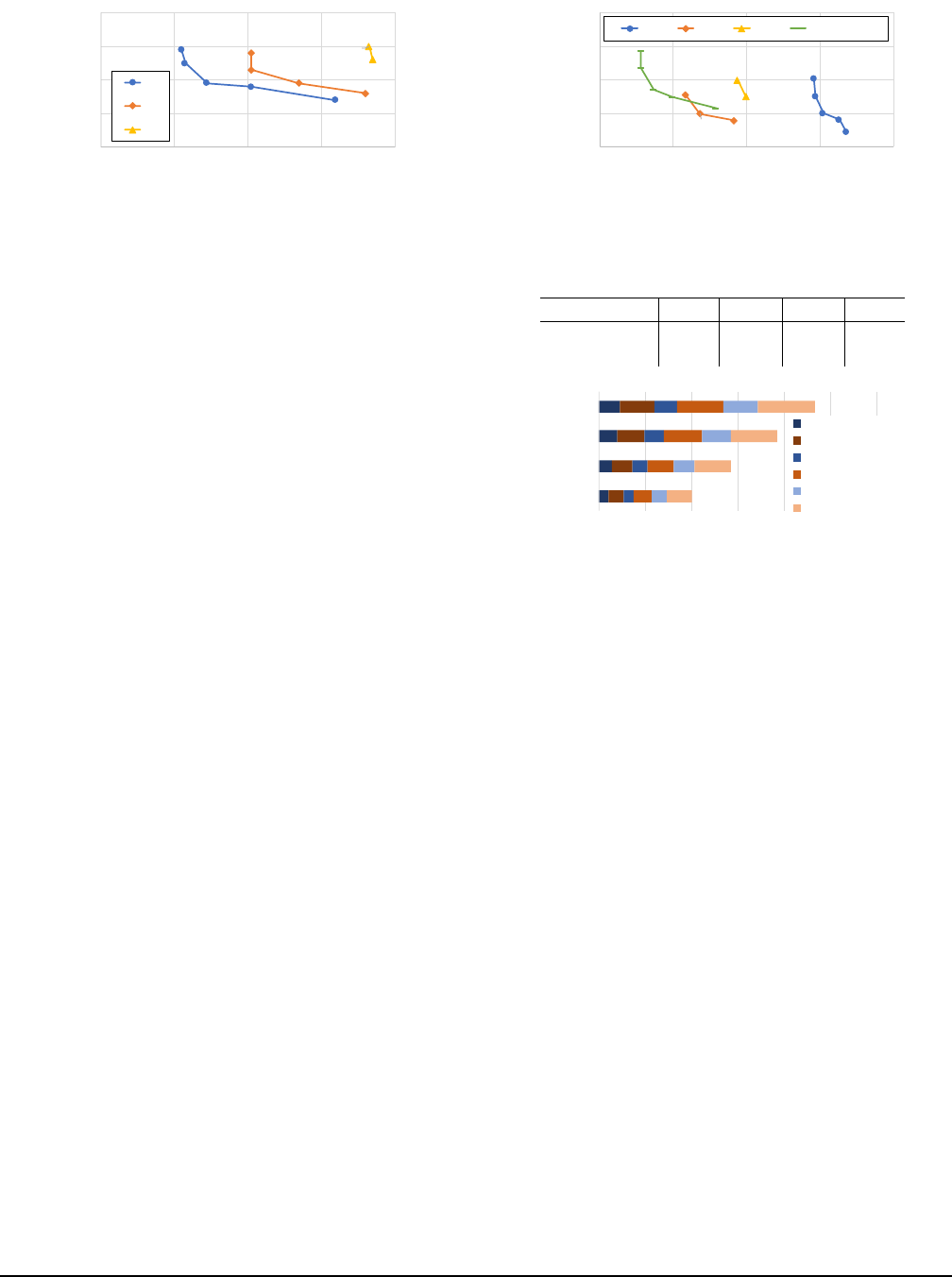
Figure 9: Running 100GB sort with Locus on a serverless in-
frastructure vs. running the same code on reserved VMs. La-
bels for serverless series represents the configured memory size
of each Lambda worker. Labels for reserved series represents
the number of c1.xlarge instances deployed.
0.01
1
100
10000
10 1000 100000 10000000
cost ($)
sort time (seconds)
S3-only
Redis-only
Hybri d
S3-only9 (predict)
Redis-only9(predict)
Hybri d9( predic t)
Figure 10: Comparing the cost and performance predicted by
Locus against actual measurements. The lines indicate pre-
dicted values and the dots indicate measurements.
of c1.xlarge instances to match the performance and com-
pare the cost. We see that both cost and performance im-
proves for Locus-serverless when we pick a smaller mem-
ory size. The performance improvement is due to increase
in parallelism that results in more aggregate network band-
width. The cost reduction comes from both shorter run-time
and lower cost for small memory sizes. For Locus-reserved,
performance improves with more instances while the cost re-
mains relatively constant, as the reduction in run-time com-
pensates for the increased allocation.
We see that even though AWS Lambda is considered to
be more expensive in terms of $ per CPU cycle, it can be
cheaper in terms of $ per Gbps compared to reserved in-
stances. Thus, serverless environments can reach a better
202 16th USENIX Symposium on Networked Systems Design and Implementation USENIX Association
0.5G
1G
1.5G
2.5G
3G
1.5G
2G
2.5G
3G
2.5G
3G
0
0.01
0.02
0.03
0.04
0 20 40 60 80
cost ($)
sort time (seconds)
40
20
10
Figure 11: 10GB slow storage-only sort, with varying paral-
lelism (lines) and worker memory size (dots).
cost performance point for network-intensive workloads.
5.3 How much fast storage is needed?
One key insight in formulating the shuffle performance in
Locus is that adding more resources does not necessarily in-
crease total cost, e.g., increasing parallelism can result in a
better configuration. Another key insight is that using fast
storage or memory, sometimes even a small amount, can sig-
nificantly shift resource balance and improve performance.
We highlight the first effect with an example of increasing
parallelism and hence over allocating worker memory com-
pared to the data size being processed. Consider the case
where we do a slow storage-only sort for 10GB. Here, we
can further increase parallelism by using smaller data parti-
tions than the worker memory size. We find that by say using
a parallelism of 40 with 2.5G worker memory size can result
in 3.21⇥ performance improvement and lower cost over us-
ing parallelism of 10 with 2.5G worker memory (Figure 11).
However, such performance increase does require that we
add resources in a balanced manner as one could also end up
incurring more cost while not improving performance. For
example, with a 100GB sort (Figure 12), increasing paral-
lelism from 200 to 400 with 2.5G worker memory size (Fig-
ure 12) makes performance 2.5⇥ worse, as now the bottle-
neck shifts to object store throughput and each worker will
run slower due to a even smaller share. Compared to the
10GB sort, this also shows that the same action that helps in
one configuration can be harmful in another configuration.
Another way of balancing resources here is to increase
parallelism while adding fast storage. We see this in Fig-
ure 12, where increasing parallelism to 400 becomes benefi-
cial with fast storage as the storage system can now absorb
the increased number of requests. These results provide an
example of the kinds of decisions automated by the perfor-
mance modeling framework in Locus.
The second insight is particularly highlighted for running
100TB hybrid sort. For 100TB sort, we vary the fast storage
used from 2% to 5%, and choose parallelism for each setting
based on the hybrid shuffle algorithm. As shown in Table 7,
we see that even with 2% of memory, the 100TB sort be-
comes attainable in 2 hours. Increasing memory from 2%
to 5%, there is an almost linear reduction in terms of end-
0.5G
1G
1.5G
2.5G
3G
0.5G
1G
1.5G
2.5G
3G
1.5G
2.5G
3G
2.5G
3G
0.100
0.200
0.300
0.400
0.500
0 50 100 150 200
cost ($)
sort time (seconds)
400
200
100
4006w/6fast
Figure 12: 100GB slow storage-only sort with varying paral-
lelism (different lines) and worker memory size (dots on same
line). We include one configuration with fast-storage sort.
Table 7: 100TB Sort with different cache size.
cache 5% 3.3% 2.5% 2%
time (s) 2945 4132 5684 6850
total cost ($) 163 171 186 179
0 2000 4000 6000 8000 10000 12000
20
30
40
50
time (seconds)
number of rounds
s3-read-input
redis-write
redis-read
s3-write-block
s3-read-block
s3-write-final
Figure 13: Runtime breakdown for 100TB sort.
to-end sort time when we use larger cache size.This matches
the projection in our design discussion. Further broken down
in Figure 13, we see that the increase of cost per time unit is
compensated by reduction in end-to-end run time.
5.4 Model Accuracy
To automatically choose a cost-effective shuffle implemen-
tation, Locus relies on a predictive performance model that
can output accurate run-time and cost for any sort size and
configuration. To validate our model, we ran an exhaustive
experiment with varying sort sizes for all three shuffle im-
plementations and compared the results with the predicted
values as shown in Figure 10.
We find that Locus’s model predicts performance and cost
trends pretty well, with an average error of 16.9% for run-
time and 14.8% for cost. Among different sort implementa-
tions, predicting Redis-only is most accurate with an accu-
racy of 9.6%, then Hybrid-sort of 18.2%, and S3-only sort of
21.5%. This might due to the relatively lesser variance we
see in network bandwidth to our dedicated Redis cluster as
opposed to S3 which is a globally shared resource. We also
notice that our prediction on average under-estimates run-
time by 11%. This can be attributed to the fact that we don’t
model a number of other overheads such as variance in CPU
time, scheduling delay etc. Overall, similar to database query
optimizers, we believe that this accuracy is good enough to
make coarse grained decisions about shuffle methods to use.
USENIX Association 16th USENIX Symposium on Networked Systems Design and Implementation 203

0
500
1000
1500
2000
2500
Query 3A Query 3B Query 3C
average query time (s)
Locus-S3
Locus
Spark
Redshift
Figure 14: Big Data Benchmark
5.5 Big Data Benchmark
The Big Data Benchmark contains a query suite derived from
production databases. We consider Query 3, which is a join
query template that reads in 123GB of input and then per-
forms joins of various sizes. We evaluate Locus to see how
it performs as join size changes. We configure Locus to use
160 workers, Spark to use 5 c3.xlarge, and Redshift to use
5ds2.8xlarge, all totalling 160 cores. Figure 14 shows that
even without the benefit of elasticity, Locus performance is
within 1.75⇥ to Apache Spark and 2.02⇥ to Redshift across
all join sizes. The gap is similar to what we observe in Sec-
tion 5.1. We also see that using a default slow-storage only
configuration can be up to 4⇥ slower.
6 Related Work
Shuffle Optimizations: As a critical component in almost
all data analytics system, shuffle has always been a venue
for performance optimization. This is exemplified by Google
providing a separate service just for shuffle [23]. While most
of its technical details are unknown, the Google Cloud Shuf-
fle service shares the same idea as Locus in that it uses elas-
tic compute resources to perform shuffle externally. Modern
analytics systems like Hadoop [39] or Spark [43] often pro-
vide multiple communication primitives and sort implemen-
tations. Unfortunately, they do not perform well in a server-
less setting, as shown previously. There are many conven-
tional wisdom on how to optimize cache performance [24],
we explore a similar problem in the cloud context. Our hy-
brid sort extends on the classic idea of mergesort (see sur-
vey [17]) and cache-sensitive external sort [30, 38] to do joint
optimization on the cache size and sort algorithm. There are
also orthogonal works that focus on the network layer. For
example, CoFlow [12] and Varys [13] proposed coordinated
flow scheduling algorithms to achieve better last flow com-
pletion time. For join operations in databases, Locus relies
on existing query compilers to generate shuffle plans. Com-
piling the optimal join algorithm for a query is an extensively
studied area in databases [14], and we plan to integrate our
shuffle characteristics with database optimizers in the future.
Serverless Frameworks: The accelerated shift to server-
less has brought innovations to SQL processing [9, 5, 22,
35], general computing platforms (OpenLambda [25], AWS
Lambda, Google Cloud Functions, Azure Functions, etc.),
as well as emerging general computation frameworks [6, 18]
in the last two years. These frameworks are architected
in different ways: AWS-Lambda [6] provides a schema to
compose MapReduce queries with existing AWS services;
ExCamera [18] implemented a state machine in serverless
tasks to achieve fine-grained control; Prior work [16] has
also looked at exploiting the usability aspects to provide a
seamless interface for scaling unmodified Python code.
Database Cost Modeling: There has been extensive study
in the database literature on building cost-models for sys-
tems with multi-tier storage hierarchy [28, 27] and on tar-
geting systems that are bottlenecked on memory access [10].
Our cost modeling shares a similar framework but examines
costs in a cloud setting. The idea of dynamically allocat-
ing virtual storage resource, especially fast cache for per-
formance improvement can also be found in database liter-
ature [41]. Finally, our work builds on existing techniques
that estimate workload statistics such as partition size, cardi-
nality, and data skew [29].
7 Conclusion
With the shift to serverless computing, there have been a
number of proposals to develop general computing frame-
works on serverless infrastructure. However, due to re-
source limits and performance variations that are inherent to
the serverless model, it is challenging to efficiently execute
complex workloads that involve communication across func-
tions. In this paper, we show that using a mixture of slow but
cheap storage with fast but expensive storage is necessary
to achieve a good cost-performance trade-off. We presents
Locus, an analytics system that uses performance modeling
for shuffle operations executed on serverless architectures.
Our evaluation shows that the model used in Locus is accu-
rate and that it can achieve comparable performance to run-
ning Apache Spark on a provisioned cluster, and within 2 ⇥
slower compared to Redshift. We believe the performance
gap can be improved in the future, and meanwhile Locus can
be preferred as it requires no provisioning of clusters.
Acknowledgement
We want to thank the anonymous reviewers and our shepherd
Jana Giceva for their insightful comments. We also thank
Alexey Tumanov, Ben Zhang, Kaifei Chen, Peter Gao, Ionel
Gog, and members of PyWren Team and RISELab for read-
ing earlier drafts of the paper. This research is supported by
NSF CISE Expeditions Award CCF-1730628, and gifts from
Alibaba, Amazon Web Services, Ant Financial, Arm, Capital
One, Ericsson, Facebook, Google, Huawei, Intel, Microsoft,
Scotiabank, Splunk and VMware.
204 16th USENIX Symposium on Networked Systems Design and Implementation USENIX Association

References
[1] ANAN T HANARAYANA N ,G.,GHODSI,A.,SHENKER,
S., AND STO IC A, I. Disk-locality in datacenter com-
puting considered irrelevant. In HotOS (2011).
[2] ANAN T HANARAYANA N ,G.,HUNG,M.C.-C.,REN,
X., STO IC A,I.,WIERMAN,A.,AND YU, M. Grass:
Trimming stragglers in approximation analytics. In
NSDI (2014).
[3] ANAN T HANARAYANA N ,G.,KANDULA,S.,GREEN-
BERG,A.,STO ICA ,I.,LU,Y.,SAHA,B.,AND HAR-
RIS, E. Reining in the Outliers in Map-Reduce Clusters
using Mantri. In Proc. OSDI (2010).
[4] ANAN T HANARAYANA N ,G.,KANDULA,S.,GREEN-
BERG,A.,STO ICA ,I.,LU,Y.,SAHA,B.,AND HAR-
RIS, E. Reining in the outliers in map-reduce clusters
using mantri. In OSDI (2010).
[5] Amazon Athena. http://aws.amazon.com/
athena/.
[6] Serverless Reference Architecture: MapRe-
duce. https://github.com/awslabs/
lambda-refarch-mapreduce.
[7] Azure Blob Storage Request Limits. https://cloud.
google.com/storage/docs/request-rate.
[8] Big Data Benchmark. https://amplab.cs.
berkeley.edu/benchmark/.
[9] Google BigQuery. https://cloud.google.com/
bigquery/.
[10] BONCZ,P.A.,MANEGOLD,S.,AND KERSTEN,
M. L. Database architecture optimized for the new bot-
tleneck: Memory access. In Proceedings of the 25th
International Conference on Very Large Data Bases
(1999).
[11] CHOWDHURY,M.,AND STOIC A, I. Coflow: A Net-
working Abstraction for Cluster Applications. In Proc.
HotNets (2012), pp. 31–36.
[12] CHOWDHURY,M.,AND STO IC A, I. Coflow: A net-
working abstraction for cluster applications. In HotNets
(2012).
[13] CHOWDHURY,M.,ZHONG,Y.,AND STOI CA, I. Ef-
ficient coflow scheduling with varys. In SIGCOMM
(2014).
[14] CHU,S.,BALAZINSKA,M.,AND SUCIU, D. From
theory to practice: Efficient join query evaluation in a
parallel database system. In SIGMOD (2015).
[15] DEAN,J.,AND GHEMAWAT, S. MapReduce: Simpli-
fied Data Processing on Large Clusters. Proc. OSDI
(2004).
[16] ERIC JONAS,QIFAN PU,SHIVARAM VENKATARA-
MAN,ION STO IC A,BENJAMIN RECHT. Occupy the
Cloud: Distributed Computing for the 99%. In SoCC
(2017).
[17] ESTIVILL-CASTRO,V.,AND WOOD, D. A survey
of adaptive sorting algorithms. ACM Comput. Surv.
(1992).
[18] FOULADI,S.,WAHBY,R.S.,SHACKLETT,B.,BAL-
ASUBRAMANIAM,K.V.,ZENG,W.,BHALERAO,R.,
SIVARAMAN,A.,PORTER,G.,AND WINSTEIN,K.
Encoding, Fast and Slow: Low-Latency Video Process-
ing Using Thousands of Tiny Threads. In NSDI (2017).
[19] GAO ,P.X.,NARAYAN,A.,KARANDIKAR,S.,CAR-
REIRA,J.,HAN,S.,AGARWAL,R.,RATNAS AM Y,S.,
AND SHENKER, S. Network requirements for resource
disaggregation. In OSDI (2016).
[20] Google Cloud Storage Request Limits. https:
//docs.microsoft.com/en-us/azure/storage/
common/storage-scalability-targets.
[21] GHEMAWAT,S.,GOBIOFF,H.,AND LEUNG, S. The
Google File System. In Proc. SOSP (2003), pp. 29–43.
[22] Amazon Glue. https://aws.amazon.com/glue/.
[23] Google Cloud Dataflow Shuffle. https://cloud.
google.com/dataflow/.
[24] GRAY,J.,AND GRAEFE, G. The five-minute rule ten
years later, and other computer storage rules of thumb.
SIGMOD Rec. (1997).
[25] HENDRICKSON,S.,STURDEVANT,S.,HARTER,T.,
VENKATARAMANI,V.,ARPACI-DUSSEAU,A.C.,
AND ARPACI-DUSSEAU, R. H. Serverless computa-
tion with OpenLambda. In HotCloud (2016).
[26] Using AWS Lambda with Kinesis. http:
//docs.aws.amazon.com/lambda/latest/dg/
with-kinesis.html.
[27] LISTGARTEN,S.,AND NEIMAT, M.-A. Modelling
costs for a mm-dbms. In RTDB (1996).
[28] MANEGOLD,S.,BONCZ,P.,AND KERSTEN,M.L.
Generic database cost models for hierarchical memory
systems. In VLDB (2002).
[29] MANNINO,M.V.,CHU,P.,AND SAGER, T. Statisti-
cal profile estimation in database systems. ACM Com-
put. Surv. (1988).
USENIX Association 16th USENIX Symposium on Networked Systems Design and Implementation 205

[30] NYBERG,C.,BARCLAY,T.,CVETANOVIC,Z.,
GRAY,J.,AND LOMET, D. Alphasort: A cache-
sensitive parallel external sort. The VLDB Journal
(1995).
[31] O’MALLEY, O. TeraByte Sort on Apache Hadoop.
http://sortbenchmark.org/YahooHadoop.pdf.
[32] OpenWhisk. https://developer.ibm.com/
openwhisk/.
[33] OUSTERHOUT,K.,RASTI,R.,RATNA SA M Y ,S.,
SHENKER,S.,AND CHUN, B.-G. Making sense of
performance in data analytics frameworks. In NSDI
(2015), pp. 293–307.
[34] POESS,M.,SMITH,B.,KOLLAR,L.,AND LARSON,
P. Tpc-ds, taking decision support benchmarking to the
next level. In SIGMOD (2002).
[35] Amazon Redshift Spectrum. https://aws.amazon.
com/redshift/spectrum/.
[36] REN,X.,ANA N T H ANAR AYANA N,G.,WIERMAN,
A., AND YU, M. Hopper: Decentralized speculation-
aware cluster scheduling at scale. SIGCOMM (2015).
[37] S3 Request Limits. https://docs.
aws.amazon.com/AmazonS3/latest/dev/
request-rate-perf-considerations.html.
[38] SALZBERG,B.,TSUKERMAN,A.,GRAY,J.,STUE-
WA RT,M.,UREN,S.,AND VAUGHAN, B. Fastsort: A
distributed single-input single-output external sort. In
SIGMOD (1990).
[39] SHVACHKO,K.,KUANG,H.,RADIA,S.,AND
CHANSLER, R. The Hadoop Distributed File Sys-
tem. In Mass storage systems and technologies (MSST)
(2010).
[40] Sort Benchmark. http://sortbenchmark.org.
[41] SOUNDARARAJAN,G.,LUPEI,D.,GHANBARI,S.,
POPESCU,A.D.,CHEN,J.,AND AMZA, C. Dynamic
resource allocation for database servers running on vir-
tual storage. In FAST (2009).
[42] WANG,Q.,GU,R.,HUANG,Y.,XIN,R.,WU,
W., SONG,J.,AND XIA, J. NADSort. http://
sortbenchmark.org/NADSort2016.pdf.
[43] ZAHARIA,M.,CHOWDHURY,M.,DAS,T.,DAV E ,
A., MA,J.,MCCAULEY,M.,FRANKLIN,M.,
SHENKER,S.,AND STO ICA , I. Resilient Distributed
Datasets: A Fault-Tolerant Abstraction for In-Memory
Cluster Computing. In Proc. NSDI (2011).
[44] ZAHARIA,M.,DAS,T.,LI,H.,SHENKER,S.,AND
STO IC A, I. Discretized streams: an efficient and fault-
tolerant model for stream processing on large clusters.
In Proceedings of the 4th USENIX conference on Hot
Topics in Cloud Ccomputing (2012), USENIX Associ-
ation.
[45] ZAHARIA,M.,KONWINSKI,A.,JOSEPH,A.D.,
KAT Z ,R.,AND STOIC A, I. Improving mapreduce
performance in heterogeneous environments. In OSDI
(2008).
206 16th USENIX Symposium on Networked Systems Design and Implementation USENIX Association
