Microsoft Word - Introduction to Pinch Technology-LinhoffMarch.doc

Introduction to Pinch

Technology

Linnhoff March

Targeting House

Gadbrook Park

Northwich, Cheshire

CW9 7UZ, England

Tel: +44 (0) 1606 815100

Fax: +44 (0) 1606 815151

[email protected]

www.linnhoffmarch.com

1 What this paper contains

This document aims to give an overview of the fundaments of Pinch Technology. The reader

will learn:

• How to obtain energy targets by the construction of composite curves.

• The three rules of the pinch principle by which energy efficient heat exchanger

network designs must abide.

• About the capital-energy trade off for new and retrofit designs.

• Of the best way to make energy saving process modifications.

• How to go about multiple utility placement.

• How best to integrate distillation columns with the background process.

• The most suitable way to integrate heat engines and heat pumps.

• The principles of data extraction.

• Some of the techniques applied in a study of a total site.

The text covers all of the aspects of the technology in PinchExpress, as well as going on to

detail theory employed in the SuperTarget suite from Linnhoff March [4]. This suite allows the

user to carry out an in depth pinch analysis, using the Process, Column and Site modules.

See the relevant pages of the Linnhoff March Web site or contact Linnhoff March for more

details.

Introduction to Pinch Technology

Table of Contents

WHAT THIS PAPER CONTAINS...................................................................................................... 1

WHAT IS PINCH TECHNOLOGY?.................................................................................................. 4

FROM FLOWSHEET TO PINCH DATA ............................................................................................5

3.1 Data Extraction Flowsheet ............................................................................................ 5

3.2 Thermal Data.................................................................................................................5

ENERGY TARGETS.....................................................................................................................6

4.1 Construction of Composite Curves ............................................................................... 6

4.2 Determining the Energy Targets ................................................................................... 7

4.3 The Pinch Principle........................................................................................................8

TARGETING FOR MULTIPLE UTILITIES .......................................................................................... 9

5.1 The Grand Composite Curve ........................................................................................ 9

5.2 Multiple Utility Targeting with the Grand Composite Curve ........................................ 11

CAPITAL - ENERGY TRADE-OFFS .............................................................................................. 12

6.1 New Designs ............................................................................................................... 12

6.2 Retrofit ......................................................................................................................... 14

PROCESS MODIFICATIONS........................................................................................................ 21

7.1 The plus-minus principle for process modifications .................................................... 21

7.2 Distillation Columns..................................................................................................... 23

PLACEMENT OF HEAT ENGINES AND HEAT PUMPS..................................................................... 26

8.1 Appropriate integration of

heat engines....................................................................... 26

8.2 Appropriate integration of heat pumps ........................................................................ 28

HEAT EXCHANGER NETWORK DESIGN ...................................................................................... 30

9.1 The Difference Between Streams and Branches........................................................ 31

9.2 The Grid Diagram for heat exchanger network representation................................... 32

9.3 The New Design Method............................................................................................. 33

9.4 Heat Exchanger Network Design for Retrofits ............................................................ 39

DATA EXTRACTION PRINCIPLES.............................................................................................. 47

10.1 Do not carry over features of the existing solution.................................................... 48

10.2 Do not mix streams at different temperatures........................................................... 49

10.3 Extract at effective temperatures............................................................................... 50

10.4 Extract streams on the safe side............................................................................... 51

10.5 Do not extract true utility streams.............................................................................. 52

10.6 Identify soft data ........................................................................................................ 52

TOTAL SITE IMPROVEMENT..................................................................................................... 53

11.1 Total site data extraction ........................................................................................... 54

11.2 Total site analysis...................................................................................................... 56

11.3 Selection of options: Total Site Road Map ................................................................ 59

REFERENCES ........................................................................................................................ 62

List of Figures

IGURE 1: "ONION DIAGRAM" OF HIERARCHY IN PROCESS DESIGN................................................... 4

IGURE 2: DATA EXTRACTION FOR PINCH ANALYSIS.......................................................................5

IGURE 3: CONSTRUCTION OF COMPOSITE CURVES....................................................................... 7

IGURE 4: USING THE HOT AND COLD COMPOSITE CURVES TO DETERMINE THE ENERGY TARGETS .....7

IGURE 5: THE PINCH PRINCIPLE .................................................................................................. 8

IGURE 6: USING COMPOSITE CURVES FOR MULTIPLE UTILITIES TARGETING .................................. 9

IGURE 7: CONSTRUCTION OF THE GRAND COMPOSITE CURVE ....................................................10

IGURE 8: USING THE GRAND COMPOSITE CURVE FOR MULTIPLE UTILITIES TARGETING ................ 11

IGURE 9: VERTICAL HEAT TRANSFER BETWEEN THE COMPOSITE CURVES LEADS TO MINIMUM

NETWORK SURFACE AREA

.................................................................................................... 13

IGURE 10: THE TRADE-OFF BETWEEN ENERGY AND CAPITAL COSTS GIVES THE OPTIMUM DTMIN FOR

MINIMUM COST IN NEW DESIGNS

........................................................................................... 14

IGURE 11: CAPITAL ENERGY TRADE OFF FOR RETROFIT APPLICATIONS......................................... 15

FIGURE 12: AREA EFFICIENCY CONCEPT...................................................................................... 16

IGURE 13: TARGETING FOR RETROFIT APPLICATIONS .................................................................. 16

Introduction to Pinch Technology

FIGURE 14: TARGETING FOR RETROFIT APPLICATIONS...................................................................17

IGURE 15: EFFECT OF SHAPE OF COMPOSITE CURVES ON OPTIMUM PROCESS DTMIN....................19

IGURE 16: MODIFYING THE PROCESS,

(A) THE +/- PRINCIPLE FOR PROCESS MODIFICATIONS (B)

TEMPERATURE CHANGES CAN AFFECT THE ENERGY TARGETS ONLY IF STREAMS ARE SHIFTED

THROUGH THE PINCH

............................................................................................................22

IGURE 17: PROCEDURE FOR OBTAINING COLUMN GRAND COMPOSITE CURVE..............................23

IGURE 18: USING COLUMN GRAND COMPOSITE CURVE TO IDENTIFY COLUMN MODIFICATIONS.......24

IGURE 19: APPROPRIATE INTEGRATION OF A DISTILLATION COLUMN WITH THE BACKGROUND

PROCESS

............................................................................................................................25

IGURE 20: APPROPRIATE PLACEMENT PRINCIPLE FOR HEAT ENGINES ..........................................27

IGURE 21: PLACEMENT OF STEAM AND GAS TURBINES AGAINST THE GRAND COMPOSITE CURVE.....28

IGURE 22: PLACEMENT OF HEAT PUMPS. ....................................................................................29

IGURE 23: A POINTED ‘NOSE’ AT THE PROCESS OR UTILITY PINCH INDICATES A GOOD HEAT PUMP

OPPORTUNITY

......................................................................................................................30

IGURE 24: KEY STEPS IN PINCH TECHNOLOGY............................................................................30

IGURE 25: THE GRID DIAGRAM FOR EASIER REPRESENTATION OF THE HEAT EXCHANGER NETWORK32

IGURE 26: GRID DIAGRAM FOR THE EXAMPLE PROBLEM ...............................................................33

IGURE 27: CRITERIA FOR TEMPERATURE FEASIBILITY AT THE PINCH..............................................34

IGURE 28: NETWORK DESIGN BELOW THE PINCH .........................................................................35

IGURE 29: COMPLETED MER NETWORK DESIGN BASED ON PINCH DESIGN METHOD ......................36

IGURE 30: CRITERIA FOR STREAM SPLITTING AT THE PINCH BASED ON NUMBER OF STREAMS AT THE

PINCH

..................................................................................................................................36

IGURE 31: INCOMING STREAM SPLIT TO COMPLY WITH CP

OUT

= CP

RULE......................................37

IGURE 32: A SUMMARY OF STREAM SPLITTING PROCEDURE DURING NETWORK DESIGN..................37

IGURE 33: A HEAT LOAD LOOP ...................................................................................................37

IGURE 34: A HEAT LOAD PATH....................................................................................................38

IGURE 35: USING A PATH TO REDUCE UTILITY USE.......................................................................38

IGURE 36: HIERARCHY OF RETROFIT DESIGN ..............................................................................40

IGURE 37: DELETE EXISTING NETWORK BEFORE APPLYING THE PINCH DESIGN METHOD................40

IGURE 38: PROCEDURE FOR CORRECTING CROSS-PINCH EXCHANGERS........................................41

IGURE 39: EXAMPLE FOR RETROFIT DESIGN USING CROSS-PINCH ANALYSIS ................................41

IGURE 40: PINCHES REPORT INDICATE THAT THE MOST SIGNIFICANT PINCH REGION IS U:377.09

(HP-STEAM (GEN))..............................................................................................................42

IGURE 41: THE LARGEST PENALTY AT U:377.09 IS EXCHANGER FDEF.........................................42

IGURE 42: THE BENEFIT REPORTED AFTER DELETING EXCHANGER FDEF AND COOLER Q_D6.......43

IGURE 43: THE SAVINGS ACHIEVED AFTER COMPLETING THE DESIGN ............................................43

IGURE 44: EXAMPLE REQUIRING PATH ANALYSIS FOR RETROFIT DESIGN ......................................45

IGURE 45: PARALLEL COMPOSITE CURVES WITH NO INTERMEDIATE UTILITIES................................45

IGURE 46: PATHS IN THE EXISTING NETWORK..............................................................................46

IGURE 47: MODIFYING TWO PATHS SAVES 14.74MMKCAL/H........................................................46

IGURE 48: DRAG AND DROP OF EXCHANGER TO A NEW POSITION IMPROVES DRIVING FORCE ON PATH

EXCHANGERS

......................................................................................................................46

IGURE 49: WITH DRIVING FORCES IMPROVED, THE TWO PATHS CAN NOW BE USED TO ACHIEVE THE

FULL SAVINGS POTENTIAL

.....................................................................................................47

IGURE 50: FINAL RETROFIT NETWORK. .......................................................................................47

IGURE 51: EXAMPLE PROCESS FLOWSHEET ...............................................................................48

IGURE 52: ORIGINAL DATA EXTRACTION AND DESIGN .................................................................49

IGURE 53: IMPROVED DATA EXTRACTION AND DESIGN ................................................................49

IGURE 54: MIXING AT DIFFERENT TEMPERATURES MAY INVOLVE IN-EFFICIENT CROSS-PINCH HEAT

TRANSFER THUS INCREASING THE ENERGY REQUIREMENT

......................................................50

IGURE 55: ISOTHERMAL MIXING AVOIDS CROSS-PINCH HEAT TRANSFER SO DO NOT MIX AT DIFFERENT

TEMPERATURES

...................................................................................................................50

IGURE 56: EVERY STREAM MUST BE EXTRACTED AT THE TEMPERATURE AT WHICH IT IS AVAILABLE TO

OTHER PROCESS STREAMS

...................................................................................................51

FIGURE 57: STREAM LINEARISATION,

A) AND B) COULD BE INFEASIBLE, C) IS SAFE SIDE LINEARISATION.52

IGURE 58: STREAM DATA EXTRACTION FOR “SOFT DATA”. ............................................................53

IGURE 59: SCHEMATIC OF A SITE, SHOWING PRODUCTION PROCESSES WHICH ARE OPERATED

SEPARATELY FROM EACH OTHER BUT ARE LINKED INDIRECTLY THROUGH THE UTILITY SYSTEM

..54

FIGURE 60: CONSTRUCTION OF TOTAL SITE PROFILES FROM PROCESS GRAND COMPOSITE CURVES55

IGURE 61: TOTAL SITE TARGETING FOR FUEL, CO-GENERATION, EMISSIONS AND COOLING .............56

Introduction to Pinch Technology

FIGURE 62: EXISTING SITE .......................................................................................................... 57

IGURE 63: PROPOSED EXPANSION OF THE SITE INVOLVING ADDITION OF A NEW PROCESS ............. 58

IGURE 64: ALTERNATIVE OPTION BASED ON TOTAL SITE PROFILES..............................................58

IGURE 65: TOTAL SITE ROAD MAP............................................................................................. 60

IGURE 66: KEY STEPS IN TOTAL SITE IMPROVEMENT.................................................................... 60

2 What is Pinch Technology?

Pinch Technology provides a systematic methodology for energy saving in processes and

total sites. The methodology is based on thermodynamic principles. Figure 1 illustrates the

role of Pinch Technology in the overall process design. The process design hierarchy can be

represented by the “onion diagram” [2, 3] as shown below. The design of a process starts

with the reactors (in the “core” of the onion). Once feeds, products, recycle concentrations

and flowrates are known, the separators (the second layer of the onion) can be designed.

The basic process heat and material balance is now in place, and the heat exchanger

network (the third layer) can be designed. The remaining heating and cooling duties are

handled by the utility system (the fourth layer). The process utility system may be a part of a

centralised site-wide utility system.

Figure 1: "Onion Diagram" of hierarchy in process design

A Pinch Analysis starts with the heat and material balance for the process. Using Pinch

Technology, it is possible to identify appropriate changes in the core process conditions that

can have an impact on energy savings (onion layers one and two). After the heat and material

balance is established, targets for energy saving can be set prior to the design of the heat

exchanger network. The Pinch Design Method ensures that these targets are achieved during

the network design. Targets can also be set for the utility loads at various levels (e.g. steam

and refrigeration levels). The utility levels supplied to the process may be a part of a

centralised site-wide utility system (e.g. site steam system). Pinch Technology extends to the

site level, wherein appropriate loads on the various steam mains can be identified in order to

minimise the site wide energy consumption. Pinch Technology therefore provides a

consistent methodology for energy saving, from the basic heat and material balance to the

total site utility system.

Introduction to Pinch Technology

3 From Flowsheet to Pinch Data

PinchExpress carries out automatic data extraction from a converged simulation. What

follows here is a brief overview of how flowsheet data are used in pinch analysis. Data

extraction is covered in more depth in "Data Extraction Principles" in section 10.

3.1 Data Extraction Flowsheet

Data extraction relates to the extraction of information required for Pinch Analysis from a

given process heat and material balance. Figure 2(a) shows an example process flow-sheet

involving a two stage reactor and a distillation column. The process already has heat

recovery, represented by the two process to process heat exchangers. The hot utility demand

of the process is 1200 units (shown by H) and the cold utility demand is 360 units (shown by

C). Pinch Analysis principles will be applied to identify the energy saving potential (or target)

for the process and subsequently to aid the design of the heat exchanger network to achieve

that targeted saving.

Figure 2: Data Extraction for Pinch Analysis

In order to start the Pinch Analysis the necessary thermal data must be extracted from the

process. This involves the identification of process heating and cooling duties. Figure 2(b)

shows the flow-sheet representation of the example process which highlights the heating and

cooling demands of the streams without any reference to the existing exchangers. This is

called the data extraction flow-sheet representation. The reboiler and condenser duties have

been excluded from the analysis for simplicity. In an actual study however, these duties

should be included. The assumption in the data extraction flow-sheet is that any process

cooling duty is available to match against any heating duty in the process. No existing heat

exchanger is assumed unless it is excluded from Pinch Analysis for specific reasons.

3.2 Thermal Data

Introduction to Pinch Technology

Table 1: Thermal Data required for Pinch Analysis

Table 1 shows the thermal data for Pinch Analysis. “Hot steams” are the streams that need

cooling (i.e. heat sources) while “cold streams” are the streams that need heating (i.e. heat

sinks). The supply temperature of the stream is denoted as Ts and target temperature as Tt.

The heat capacity flow rate (CP) is the mass flowrate times the specific heat capacity i.e.

CP = Cp x M

where Cp is the specific heat capacity of the stream (KJ/ºC, kg) and M is the mass flowrate

(kg/sec). The CP of a stream is measured as enthalpy change per unit temperature (kW/ºC or

equivalent units). For this example a minimum temperature difference of 10ºC is assumed

during the analysis which is the same as in the existing process, as highlighted in Figure 2(a).

The hot utility is steam available at 200ºC and the cold utility is cooling water available

between 25ºC to 30ºC.

4 Energy Targets

Starting from the thermal data for a process (such as shown in Table 1), Pinch Analysis

provides a target for the minimum energy consumption. The energy targets are obtained

using a tool called the “Composite Curves”.

4.1 Construction of Composite Curves

Composite Curves consist of temperature-enthalpy (T-H) profiles of heat availability in the

process (the “hot composite curve”) and heat demands in the process (the “cold composite

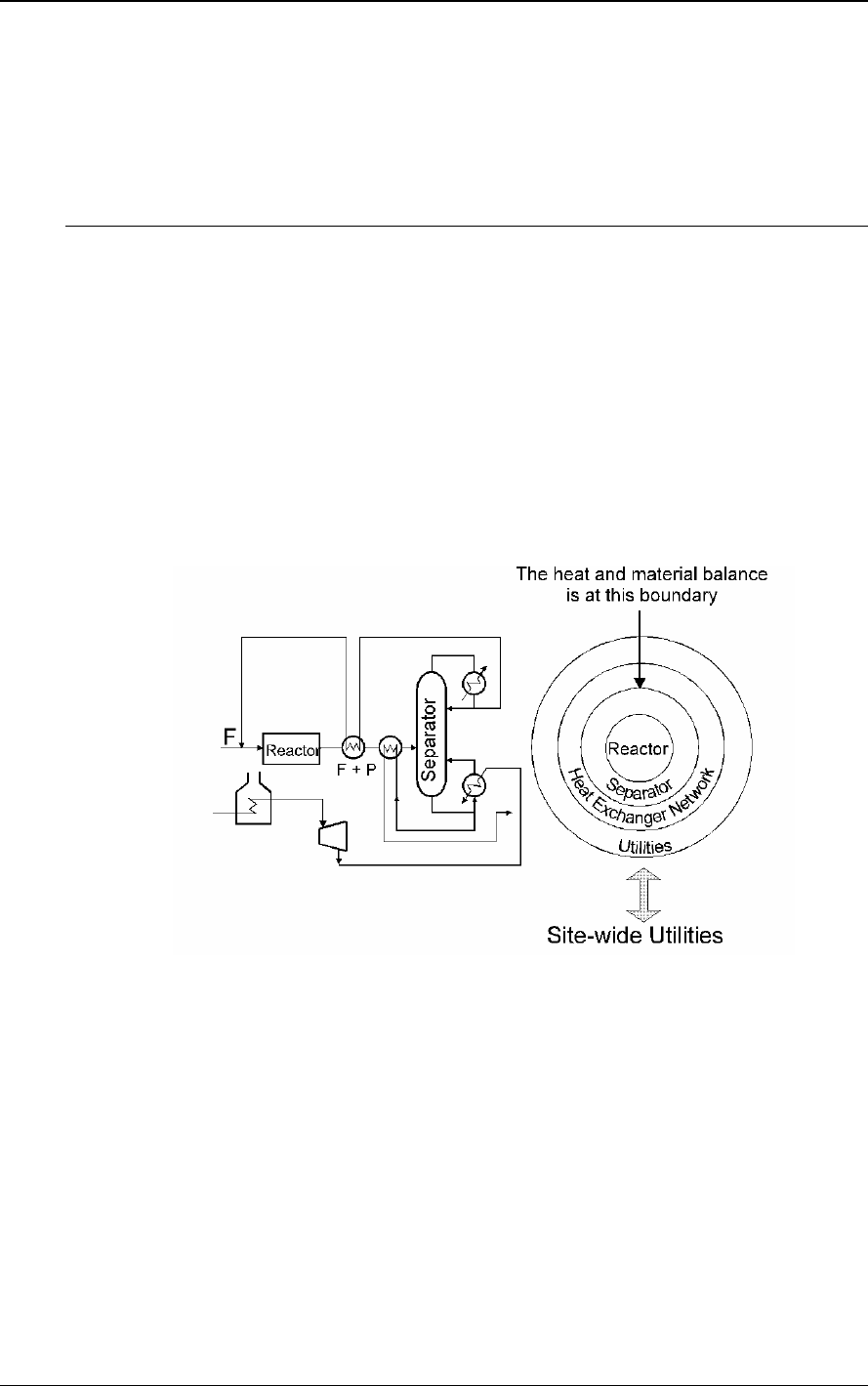
curve”) together in a graphical representation. Figure 3 illustrates the construction of the “hot

composite curve” for the example process, which has two hot streams (stream number 1 and

2, see Table 1). Their T-H representation is shown in Figure 3(a) and their composite

representation is shown in Figure 3(b). Stream 1 has a CP of 20 kW/°C, and is cooled from

180°C to 80°C, releasing 2000kW of heat. Stream 2 is cooled from 130°C to 40°C and with a

CP of 40kW/°C and loses 3600kW.

Introduction to Pinch Technology

Figure 3: Construction of Composite Curves

The construction of the hot composite curve (as shown in Figure 3(b)) simply involves the

addition of the enthalpy changes of the streams in the respective temperature intervals. In the

temperature interval 180ºC to 130ºC only stream 1 is present. Therefore the CP of the

composite curve equals the CP of stream 1 i.e. 20. In the temperature interval 130ºC to 80ºC,

both streams 1 and 2 are present, therefore the CP of the hot composite equals the sum of

the CP’s of the two streams i.e. 20+40=60. In the temperature interval 80ºC to 40ºC only

stream 2 is present, thus the CP of the composite is 40. The construction of the cold

composite curve is similar to that of the hot composite curve involving the combination of the

cold stream T-H curves for the process.

4.2 Determining the Energy Targets

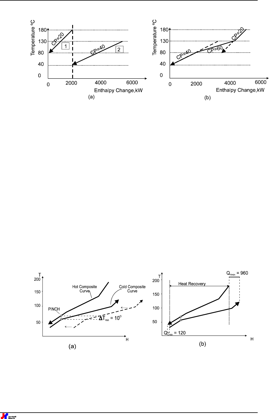
The composite curves provide a counter-current picture of heat transfer and can be used to

indicate the minimum energy target for the process. This is achieved by overlapping the hot

and cold composite curves, as shown in Figure 4(a), separating them by the minimum

temperature difference DT

min

(10ºC for the example process).

This overlap shows the

maximum process heat recovery possible (Figure 4(b)), indicating that the remaining heating

and cooling needs are the minimum hot utility requirement (Q

Hmin

) and the minimum cold

utility requirement (Q

Cmin

) of the process for the chosen

min

Figure 4: Using the hot and cold composite curves to determine the energy targets

The composite curves in Figure 4 have been constructed for the example process (Figure 2

and Table 1). The minimum hot utility (Q

Hmin

)

for the example problem is 960 units which is

less than the existing process energy consumption of 1200 units. The potential for energy

saving is therefore 1200-960 = 240 units by using the same value of DT

min

as the existing

Introduction to Pinch Technology

process. Using Pinch Analysis, targets for minimum energy consumption can be set purely on

the basis of heat and material balance information, prior to heat exchanger network design.

This allows quick identification of the scope for energy saving at an early stage.

4.3 The Pinch Principle

The point where DT

min

is observed is known as the “Pinch” and recognising its implications

allows energy targets to be realised in practice.

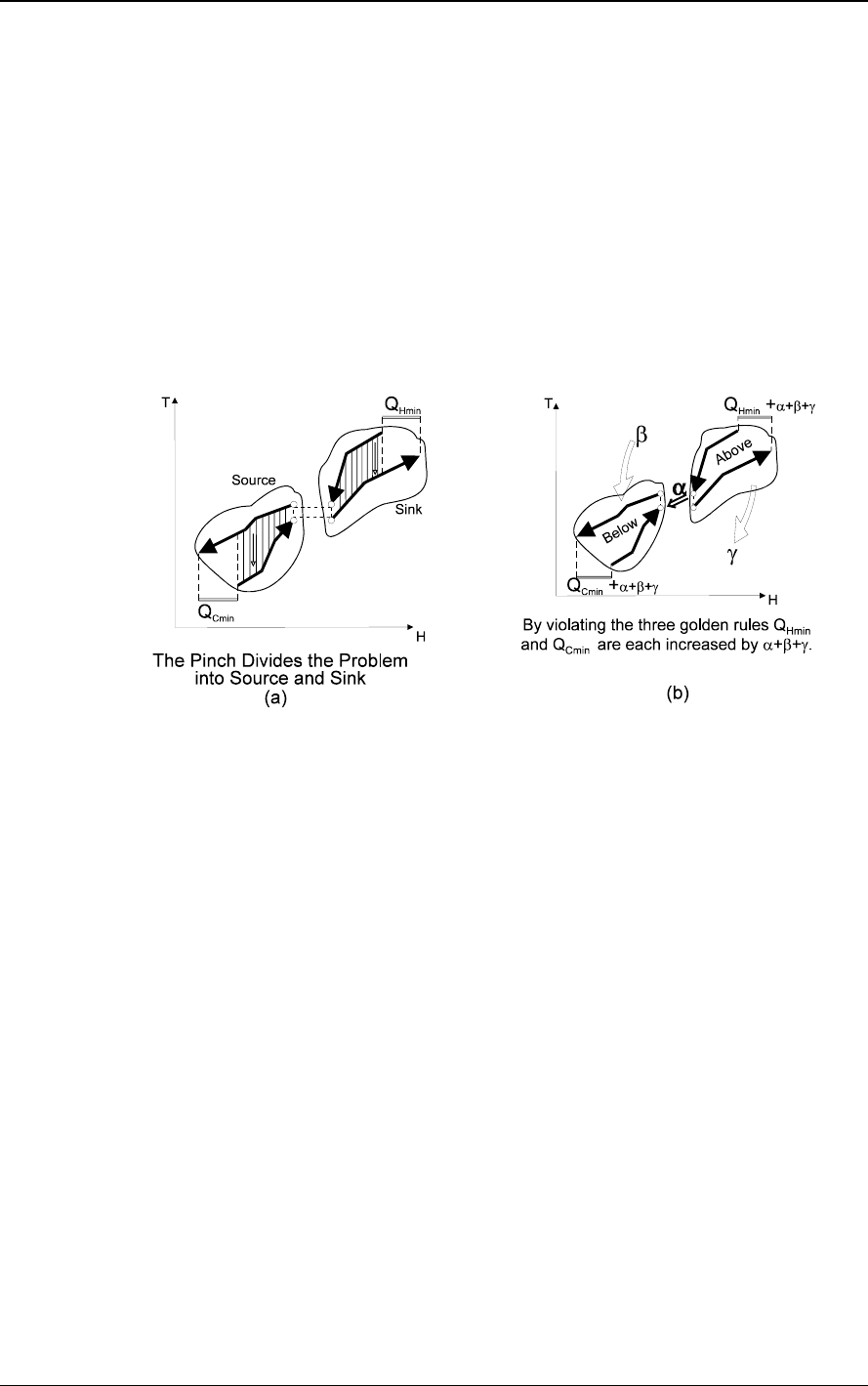
Once the pinch has been identified, it is

possible to consider the process as two separate systems: one above and one below the

pinch, as shown in Figure 5(a).

The system above the pinch requires a heat input and is

therefore a net heat sink.

Below the pinch, the system rejects heat and so is a net heat

source.

Figure 5: The Pinch Principle

In Figure 5(b), α amount of heat is transferred from above the pinch to below the pinch. The

system above the pinch, which was before in heat balance with Q

Hmin

, now loses α units of

heat to the system below the pinch. To restore the heat balance, the hot utility must be

increased by the same amount, that is, α units. Below the pinch, α units of heat are added to

the system that had an excess of heat, therefore the cold utility requirement also increases by

α units. In conclusion, the consequence of a cross-pinch heat transfer (α) is that both the hot

and cold utility will increase by the cross-pinch duty (α).

For the example process (Figure 2, Figure 4) the cross pinch heat transfer in the existing

process is equal to 1200-960 = 240 units.

Figure 5(b) also shows γ amount of external cooling above the pinch and β amount of

external heating below the pinch. The external cooling above the pinch of γ amount increases

the hot utility demand by the same amount. Therefore on an overall basis both the hot and

cold utilities are increased by γ amount. Similarly external heating below the pinch of β

amount increases the overall hot and cold utility requirement by the same amount (i.e. β).

To summarise, the understanding of the pinch gives three rules that must be obeyed in order

to achieve the minimum energy targets for a process:

• Heat must not be transferred across the pinch

• There must be no external cooling above the pinch

Introduction to Pinch Technology

• There must be no external heating below the pinch

Violating any of these rules will lead to cross-pinch heat transfer resulting in an increase in

the energy requirement beyond the target. The rules form the basis for the network design

procedure which is described in "Heat Exchanger Network Design" section 9. The design

procedure for heat exchanger networks ensures that there is no cross pinch heat transfer. For

retrofit applications the design procedure “corrects” the exchangers that are passing the heat

across the pinch.

5 Targeting for Multiple Utilities

The energy requirement for a process is supplied via several utility levels e.g. steam levels,

refrigeration levels, hot oil circuit, furnace flue gas etc. The general objective is to maximise

the use of the cheaper utility levels and minimise the use of the expensive utility levels. For

example, it is preferable to use LP steam instead of HP steam, and cooling water instead of

refrigeration. The composite curves provide overall energy targets but do not clearly indicate

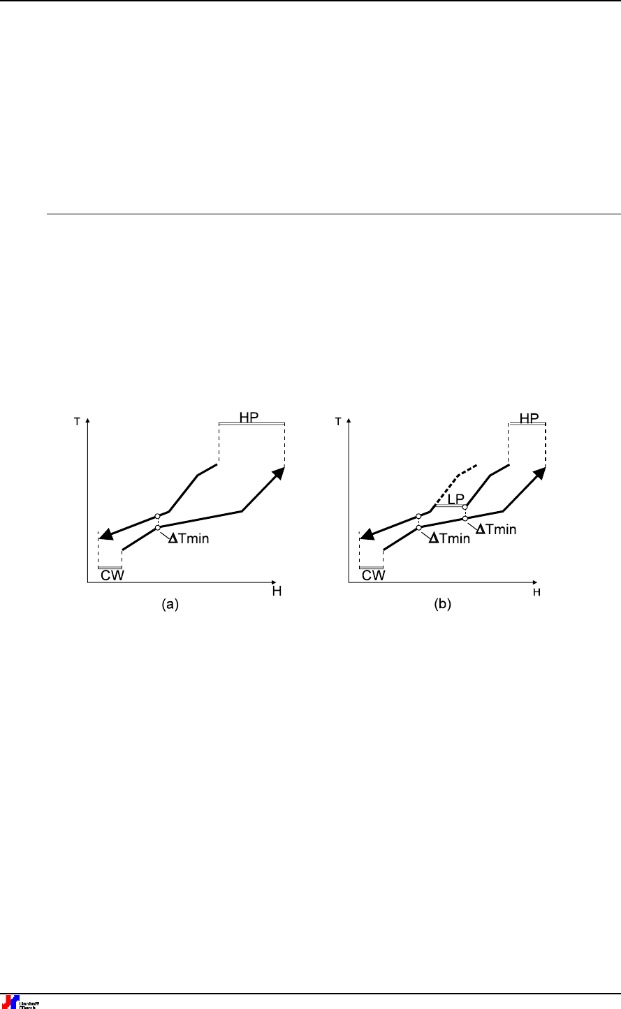
how much energy needs to be supplied by different utility levels. This is illustrated in Figure 6.

Figure 6: Using Composite Curves for Multiple Utilities Targeting

The composite curves in Figure 6(a) provide targets for the extreme utility levels HP steam

and cooling water.

Figure 6(b) shows the construction of the composite curves if LP steam

consumption replaces part of the HP steam consumption. The LP steam load is added to the

hot composite curve as shown in Figure 6(b). As the LP steam consumption increases a

min

temperature difference is reached between the composite curves. This is the maximum

LP consumption that can replace the HP steam consumption.

Every time a new utility level is

added, the same procedure would have to be repeated in order to set the load on the new

utility level. The shape of the composite curves will change with every new utility level

addition and the overall construction becomes quite complex for several utility levels. The

composite curves are therefore a difficult tool for setting loads for the multiple utility levels.

What is required is a clear visual representation of the selected utilities and the associated

enthalpy change without the disadvantages of using composite curves. For this purpose, the

Grand Composite Curve is used.

5.1 The Grand Composite Curve

Introduction to Pinch Technology

The tool that is used for setting multiple utility targets is called the Grand Composite Curve,

the construction of which is illustrated in Figure 7. This starts with the composite curves as

shown in Figure 7(a). The first step is to make adjustments in the temperatures of the

composite curves as shown in Figure 7(b). This involves increasing the cold composite

temperature by ½ DT

min

and

decreasing the hot composite temperature by ½ DT

min

This temperature shifting of the process streams and utility levels ensures that even when the

utility levels touch the grand composite curve, the minimum temperature difference of DT

min

maintained between the utility levels and the process streams. The temperature shifting

therefore makes it easier to target for multiple utilities. As a result of this temperature shift, the

composite curves touch each other at the pinch. The curves are called the “shifted composite

curves”.

The grand composite curve is then constructed from the enthalpy (horizontal)

differences between the shifted composite curves at different temperatures (shown by

distance α in Figure 7(b) and (c)). The grand composite curve provides the same overall

energy target as the composite curves, the HP and refrigeration (ref.) targets are identical in

Figure 7(a) and (c).

Figure 7: Construction of the Grand Composite Curve

The grand composite curve indicates “shifted” process temperatures. Since the hot process

streams are reduced by ½ DT

min

and cold process streams are increased by

½ DT

min

the

construction of the grand composite curve automatically ensures that there is at least DT

min

temperature difference between the hot and cold process streams.

The utility levels when

placed against the grand composite curve are also shifted by ½ DT

min

- hot utility

temperatures decreased by ½ DT

min

and cold utility temperatures increased by ½ DT

min

For

instance steam used at 200ºC will be shown at 190ºC if the DT

min

is 20ºC.

This shifting of

utilities temperatures ensures that there is a minimum temperature difference of DT

min

between the utilities and the corresponding process streams. More importantly, when utility

levels touch the grand composite curve, DT

min

temperature difference is maintained.

In PinchExpress there is a further refinement of this approach whereby the utilities are shifted

by an amount that guarantees a user-specified approach temperature between the utility and

the process streams. This approach temperature does not have to be the same as the

process DTmin and can be different for each utility. For example, this is typically set at 40ºC

for flue gas, between 10ºC and 20ºC for steam and about 3ºC for low temperature

Introduction to Pinch Technology

refrigeration. For more details see the section "Typical DTmin values for matching utility levels

against process streams" on page 20.

5.2 Multiple Utility Targeting with the Grand Composite Curve

The grand composite curve provides a convenient tool for setting the targets for the multiple

utility levels as illustrated in Figure 8.

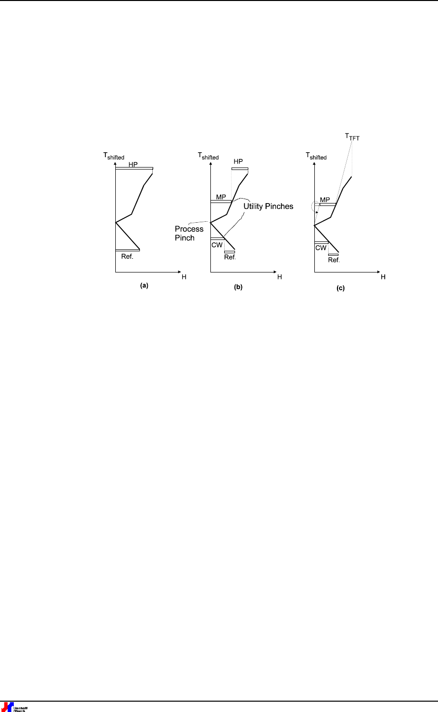
Figure 8: Using the Grand Composite Curve for Multiple Utilities Targeting

Figure 8(a) shows a situation where HP steam is used for heating and refrigeration is used for

cooling the process. In order to reduce the utilities cost, intermediate utilities MP steam and

cooling water (CW) are introduced. Figure 8(b) shows the construction on the grand

composite curve providing targets for all the utilities. The target for MP steam is set by simply

drawing a horizontal line at the MP steam temperature level starting from the vertical (shifted

temperature) axis until it touches the grand composite curve. The remaining heating duty is

then satisfied by the HP steam.

This maximises the MP consumption prior to the use of the

HP steam and therefore minimises the total utilities cost. Similar construction is performed

below the pinch to maximise the use of cooling water prior to the use of refrigeration as

shown in Figure 8(b).

The points where the MP and CW levels touch the grand composite curve are called the

“Utility Pinches” since these are caused by utility levels. A violation of a utility pinch (cross

utility pinch heat flow) results in shifting of heat load from a cheaper utility level to a more

expensive utility level. A “Process Pinch” is caused by the process streams, and as discussed

earlier (in "The Pinch Principle" section 4.3), violation of a process pinch results in an overall

heat load penalty for the utilities.

Figure 8(c) shows a different possibility of utility levels where furnace heating is used instead

of HP steam. Considering that furnace heating is more expensive than MP steam, the use of

MP steam is maximised. In the temperature range above the MP steam level, the heating

duty has to be supplied by the furnace flue gas. The flue gas flowrate is set as shown in

Figure 8(c) by drawing a sloping line starting from the MP steam temperature to theoretical

flame temperature (T

TFT

). If the process pinch temperature is above the flue gas corrosion

temperature, the heat available from the flue gas between MP steam and pinch temperature

can be used for process heating. This will reduce the MP steam consumption as shown in

Figure 8(c). The MP steam load needs to be adjusted accordingly.

Introduction to Pinch Technology

In summary the grand composite curve is one of the basic tools used in pinch analysis for

selection of appropriate utility levels and for targeting for a given set of multiple utility levels.

The targeting involves setting appropriate loads for the various utility levels by maximising

cheaper utility loads and minimising the loads on expensive utilities.

6 Capital - Energy Trade-offs

The best design for an energy efficient heat exchange network will often result in a trade off

between the equipment and operating costs. This is dependent on the choice of the DT

min

for

the process. The lower the DT

min

chosen, the lower the energy costs, but conversely the

higher the heat exchanger capital costs, as lower temperature driving forces in the network

will result in the need for greater area. A large DT

min

, on the other hand, will mean increased

energy costs as there will be less overall heat recovery, but the required capital costs will be

less. The trade-off is further complicated in a retrofit situation, where a capital investment has

already been made. This section explains a rational approach to the complex task of capital-

energy trade-offs.

6.1 New Designs

So far the use of Pinch Analysis has been considered for setting the energy targets for a

process. These targets are dependent on the choice of the DT

min

for the process. Lowering

the value of DT

min

lowers the target for minimum energy consumption for the process. In this

section the concept of heat exchanger network capital cost targets for the process are

discussed. For certain types of applications such as refinery crude preheat trains, where

there are few matching constraints between hot and cold streams, it is possible to set capital

cost targets in addition to the energy targets. This allows the consideration of the trade-offs

between capital and energy in order to obtain an optimum value of DT

min

ahead of network

design.

This functionality is provided in the SuperTarget Process module developed by Linnhoff March

[4].

6.1.1 Setting Area Targets

The composite curves make it possible to determine the energy targets for a given value of

min

. The composite curves can also be used to determine the minimum heat transfer area

required to achieve the energy targets:

Network Area, A

min

⎡

⎣

⎢

⎤

⎦

⎥

∑∑

∆

where:

i: denotes ith enthalpy interval

j: jth stream

∆T

: log mean temperature difference in interval

: enthalpy change of jth stream

Introduction to Pinch Technology

: heat transfer coefficient of jth stream

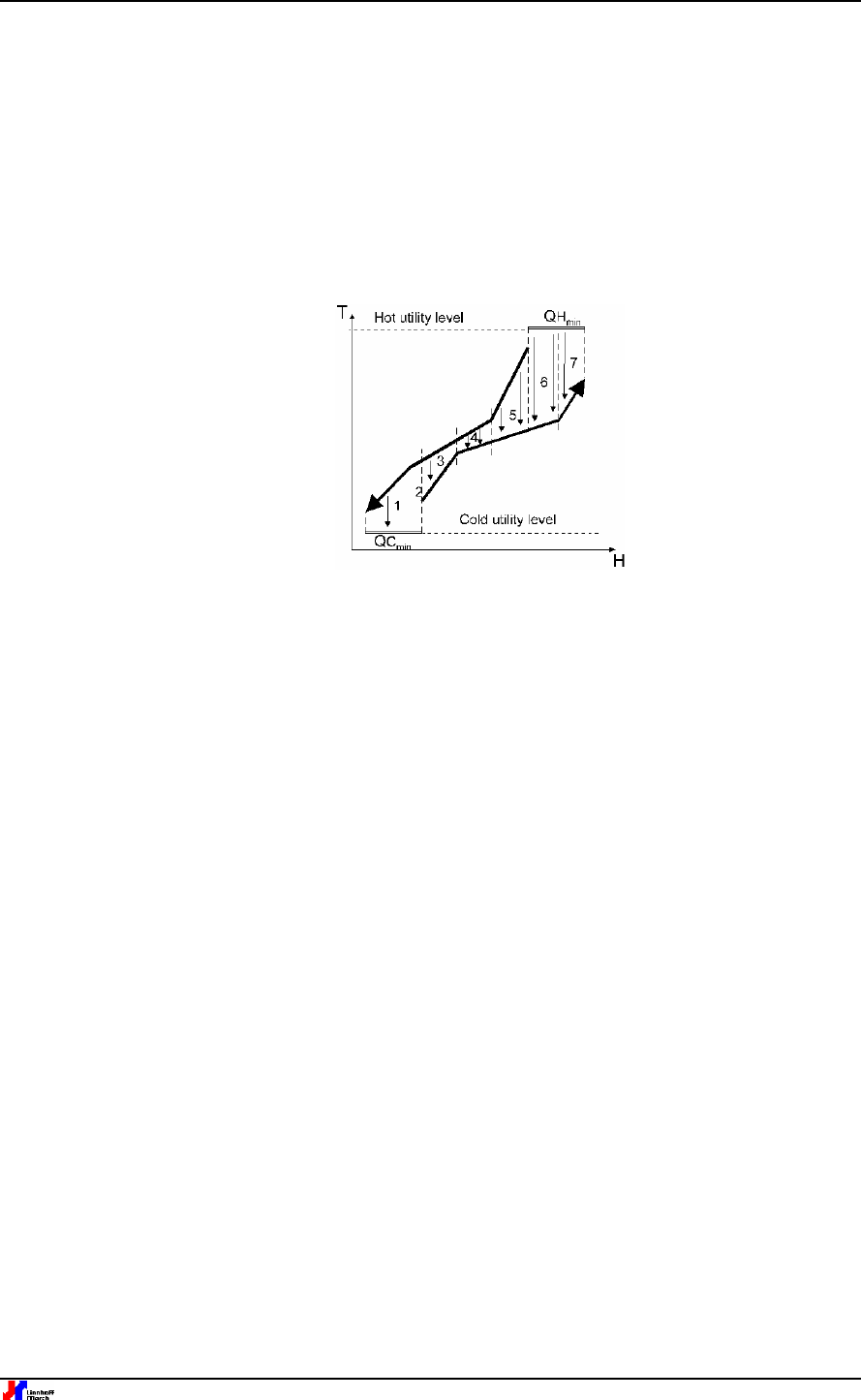
This area target is based on the assumption that “vertical” heat exchange will be adopted

between the hot and the cold composite curves across the whole enthalpy range as shown in

Figure 9. This vertical arrangement, which is equivalent to pure counter-current area within

the overall network, has been found to give a minimum total surface area. For a case where

the process streams have uniform heat transfer coefficients this is rigorous. In a new design

situation, where there are no existing exchangers, it should be possible to design a network

that is close to these targets.

Figure 9: Vertical heat transfer between the composite curves leads to minimum network

surface area

6.1.2 Setting Minimum Number of Units Target

It is also possible to set a target for the minimum number of heat exchanger units in a

process. The minimum number of heat exchange units depends fundamentally on the total

number of process and utility streams (N) involved in heat exchange. This can also be

determined prior to design by using a simplified form of Euler’s graph theorem [2, 3].

min

= N - 1

where:

min

: Minimum number of heat exchanger units

N: Total number of process and utility streams in the heat exchanger network

This equation is applied separately on each side of the pinch, as in an MER (minimum energy

requirement) network there is no heat transfer across the pinch and therefore the network is

divided into two independent problems: one above, and one below the pinch.

6.1.3 Determining the Capital Cost Target

The targets for the minimum surface area and the number of units (U

min

) can be combined

together with the heat exchanger cost law equations [8] to generate the targets for heat

exchanger network capital cost. The capital cost target can be super-imposed on the energy

cost targets to obtain the minimum total cost target for the network as shown in Figure 10.

Introduction to Pinch Technology

Figure 10: The trade-off between energy and capital costs gives the optimum DTmin for

minimum cost in new designs

This provides an optimum DT

min

for the network ahead of design [3, 8]. It is important to note

that the capital cost targeting algorithm is based on the simplifying assumption that any hot

stream can match against any cold stream. It does not consider matching constraints

between specific hot and cold streams. Therefore the capital cost targeting technique and

min

optimisation is particularly applicable for systems with fewer matching constraints such

as atmospheric and vacuum distillation preheat trains, FCC unit, etc..

The description above has assumed pure counter-current heat exchangers. However, in

SuperTarget Process there is an additional option to target based on shell and tube

exchangers with one shell pass and two tube passes. This is the most common exchanger

type found in industrial use.

6.2 Retrofit

Pinch Technology is applicable to both new design and retrofit situations. The number of

retrofit applications is much higher than the number of new design applications.

In this section techniques are discussed for setting targets for energy saving for an existing

plant based on capital-energy trade-off for retrofit projects. The SuperTarget Process module

developed by Linnhoff March [4] contains tools which employ these techniques.

6.2.1 Retrofit Targeting based on Capital-energy trade-off

Figure 11 provides an understanding of the capital - energy trade-off for a retrofit project

using an area-energy plot.

Introduction to Pinch Technology

Figure 11: Capital energy trade off for retrofit applications

The curve (enclosing the shaded area) is based on new design targets for the process. The

shaded area indicates performance better than the new design targets (which is infeasible for

an existing plant). An existing plant will typically be located above the new design curve. The

closer the existing plant is to the new design curve the better the current performance. In a

retrofit modification, for increased energy saving, the installation of additional heat exchanger

surface area is expected. The curve for the additional surface area that is closest to the new

design area-energy curve provides the most efficient route for investment (good economics).

The following section explains how such a curve for a retrofit application can be developed

ahead of design.

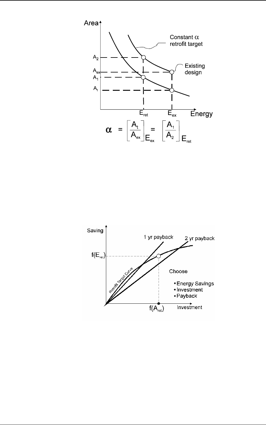
6.2.2 Maintaining Area Efficiency

Figure 12 depicts an approach for retrofit targeting based on the concept of “area efficiency”.

An area efficiency factor α can be determined for an existing network according to the

following equation:

α = [ A

/ A

]

Eex

= [A

/ A

]

Eret

where:

: Existing energy consumption

: Existing surface area of the network

: Target surface area for the new design at the existing energy consumption (E

Introduction to Pinch Technology

Figure 12: Area Efficiency concept

Area efficiency determines how close the existing network is to the new design area target. In

order to set a retrofit target, one approach is to assume that the area efficiency of the new

installed area is the same as the existing network as shown in Figure 12 [3, 9].

6.2.3 Payback

From the area-energy targeting curve the saving versus investment curve for the retrofit

targeting can be developed. This is shown in Figure 13.

Figure 13: Targeting for retrofit applications

Various pay-back lines can be established as shown in the figure. Based on the specified

pay-back or investment limit, the target energy saving can be set. This will in turn determine

the targeted DT

min

value for the network. From the target DT

min

value, the cross pinch heat

flow and the cross pinch heat exchangers that need to be corrected are calculated. This

forms the basis for the network design modification as further discussed in "Heat Exchanger

Network Design" (section 9).

This targeting procedure is based on the constant α assumption. This assumption is

particularly valid if the α for the existing network is high (say above 0.85). In situations where

Introduction to Pinch Technology

the existing α is low (say 0.6) the constant α assumption is conservative. In such cases it can

be assumed that the additional area can be installed at a higher area efficiency (say 0.9 or 1).

The retrofit targeting procedure is particularly applicable for processes with few matching

constraints such as atmospheric and vacuum distillation preheat trains. For other applications

the targeting methods described in the following sections are more applicable.

6.2.4 Retrofit targeting based on DT

min

- Energy curves

Exchanger capital cost and heat transfer information is required to set the retrofit targets

based on capital energy trade-off. In addition, the process may have heat exchanger

matching constraints which create inaccuracies in the capital cost targets as described in

"Payback" previously. Finally the project time constraints may limit the use of the capital cost

targets for retrofit targeting. In this section a simpler approach to retrofit targeting based on

the analysis of energy target variation with DT

min

is described.

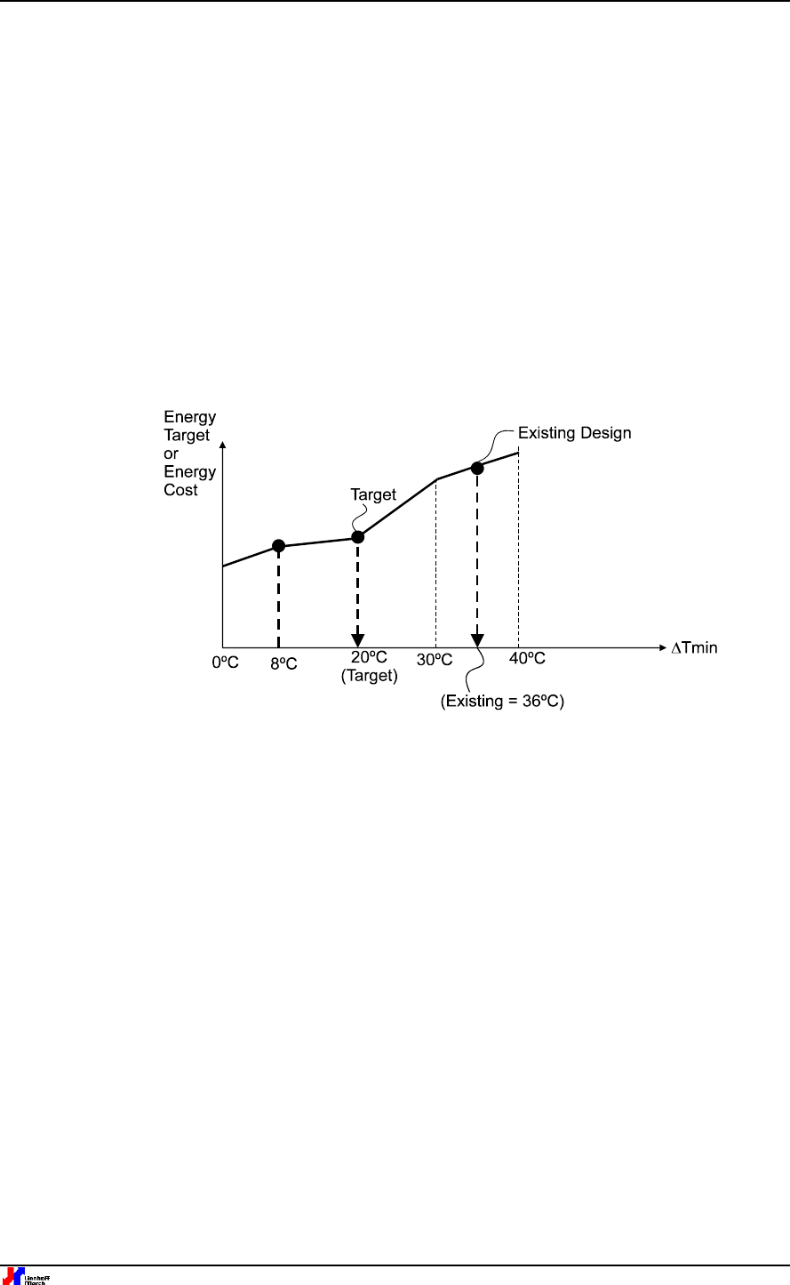
Figure 14: Targeting for retrofit applications

Figure 14 shows an example of a DT

min

- Energy plot for a process. The plot can be directly

obtained from the process composite curves. The vertical axis can represent energy target or

energy cost. Existing design corresponds to the DT

min

of 36ºC between the composite curves.

The plot shows that the variation of energy target (or energy cost) is quite sensitive to DT

min

the temperature range of 30ºC to 20ºC. However between 20ºC and 8ºC the energy target is

not sensitive to DT

min.

On the other hand the capital cost may rise substantially in this region.

It therefore implies that 20ºC is an appropriate target for the retrofit.

Although the DT

min

- Energy plot does not directly account for the capital cost dimension, it is

expected that dominant changes in the energy dimension will have an impact on the capital-

energy trade-off. The above approach, coupled with previous application experience on

similar processes (see following section: "Retrofit targeting based on experience DT

min

values") provides practical targets in many situations.

6.2.5 DTmin Calculation in PinchExpress

In PinchExpress, an option for automatically calculating a suitable DTmin for a process is

available. This calculation is done by considering an area-energy trade-off based on one of

two benchmark processes built in to PinchExpress. These processes are used as they

represent two extremes of plant economics.

Introduction to Pinch Technology

A Crude Oil Project is used as the benchmark for above ambient processes because it

displays a well behaved trade-off between area cost and capital cost. In addition, the optimum

DTmin for this process is high because the composite curves are narrow, leading to high area

requirements. This means that it represents one extreme of plant economics, where the

optimum DTmin can be greater than 30°C. Using this benchmark will ensure that a lower

DTmin is selected for an above ambient process with diverging composite curves.

An Ethylene cold-end project is used as the benchmark for below ambient processes

because it requires refrigeration utilities at temperatures as low as -100°C. This is very

expensive so the economic DTmin is sensitive to the cost of the refrigeration utilities. This

therefore represents the other extreme of plant economics, where driving forces are tight to

minimise expensive refrigeration. The optimum DTmin for an ethylene cold-end may be as

low as 2°C. Using this as a benchmark will ensure that other processes requiring less

extreme refrigeration will use a higher DTmin.

A process that is similar to one of these two will be adequately represented by the benchmark

trade-off between area cost and energy cost. This trade-off can be fine tuned by changing the

benchmark DTmin values.

For each benchmark, PinchExpress defines two different DTmin values, one for a New

Design and one for a Retrofit project. The values for retrofit are usually slightly higher than

those for New Design (i.e. saving less energy) due to the difficulty of re-arranging the existing

heat exchangers.

A process that is significantly different from either benchmark will fit into one of the following

categories:

1. It has divergent composite curves and scope for use of intermediate utilities. For these

processes the optimum DTmin is usually determined by a sharp change in the plot of

DTmin vs. Energy Cost. This means that the trade-off between Energy Cost and Capital

Cost can vary significantly without hardly changing the optimum DTmin at all. In other

words, the answer is not very sensitive to the trade-off so the benchmark values are

perfectly adequate.

2. It is a mixture of above and below ambient parts. In this case PinchExpress will

automatically use both benchmarks when determining the trade-off between energy cost

and capital cost.

From this discussion it should now be clear that PinchExpress has sufficient information to

calculate a suitable DTmin for any type of process. Most importantly, this can be done without

knowing specific information about individual heat exchanger costs or heat transfer

coefficients.

A final point worth making is that this new method can be regarded as a combination of all the

other methods described in this document, for the following reasons:

1. The use of benchmark processes is analogous to the use of experience values (see next

section).

2. For a refinery process the method will explore the trade-off between area cost and energy

cost, in a similar manner to that described in earlier sections.

Introduction to Pinch Technology

3. For a petro-chemical process the method will identify sharp changes in the plot of Energy

Cost vs. DTmin, which is the method described previously in “Retrofit targeting based on

DTmin - Energy curves”.

6.2.6 Retrofit targeting based on experience DT

min

values

It is expected that retrofit projects involving similar cost scenarios (fuel and capital costs etc.),

and similar levels of process technology may result in similar target DT

min

values.

In such

cases previous applications experience provides a useful source of information for setting the

target DT

min

for the process.

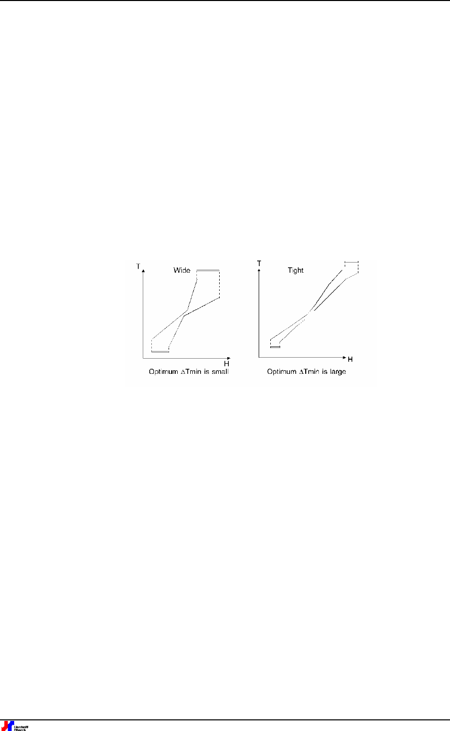
Usually similar processes have similar shapes of composite curves. For example for

atmospheric distillation units, the composite curves tend

be “parallel” to each other due to the

similarity of

the mass flows between the feed and the products of distillation. The shape of the

composite curves influences the temperature driving force distribution in the process and

therefore the heat exchanger network capital cost. Figure 15 illustrates the impact of the

shape of the composite curves on the target DT

min

value.

Figure 15: Effect of shape of composite curves on optimum process DTmin

For wide (or divergent) composite curves, even at low values of DT

min

, the overall

temperature driving force is quite high. Conversely for tight (or parallel) composite curves the

heat exchanger capital cost will be quite high at low DT

min

values. Such an understanding

coupled with previous applications experience can be quite useful in setting practical retrofit

targets.

The following tables detail Linnhoff March's experience DT

min

values. It is important to note

that although experience based DT

min

values can provide practical targets for retrofit

modifications, in certain situations it may result in non-optimal solutions and therefore loss of

potential opportunities. It is therefore recommended that the use of experience based DT

min

treated with caution and that as much as possible the choice is backed up by quantitative

information (such as DT

min

versus energy plot etc.).

Introduction to Pinch Technology

6.2.7 Typical DT

min

values for various types of processes

Table 2 shows typical

min

values for several types of processes. These are values based

on Linnhoff March’s application experience.

No Industrial Sector Experience DT

min

Values Comments

1 Oil Refining 20-40ºC Relatively low heat transfer

coefficients, parallel

composite curves in many

applications, fouling of heat

exchangers

2 Petrochemical 10-20ºC Reboiling and condensing

duties provide better heat

transfer coefficients, low

fouling

3 Chemical 10-20ºC As for Petrochemicals

4 Low Temperature Processes 3-5ºC Power requirement for

refrigeration system is very

expensive.

min

decreases

with low refrigeration

temperatures

Table 2: Typical DT

min

values for various types of processes

6.2.8 Typical DT

min

values used for matching utility levels against process

streams

Below are typical DT

min

values for matching utilities against process streams.

These

experience based DT

min

values are useful in identifying targets for appropriate utility loads at

various utility levels.

Match DT

min

Comments

Steam against Process Stream 10-20ºC Good heat transfer coefficient for steam

condensing or evaporation

Refrigeration against Process Stream 3-5ºC Refrigeration is expensive

Flue gas against Process Stream 40ºC Low heat transfer coefficient for flue gas

Flue gas against Steam Generation 25-40ºC Good heat transfer coefficient for steam

Flue gas against Air (e.g. air preheat) 50ºC Air on both sides.

Depends on acid dew

point temperature

CW against Process Stream 15-20ºC Depends on whether or not CW is

competing against refrigeration.

Summer/Winter operations should be

considered

Table 3: Typical DT

min

values for process-utility matches

Introduction to Pinch Technology

6.2.9 Typical DT

min

values used in retrofit targeting of various refinery

processes

Table 4 shows typical DT

min

values used in retrofit targeting of refinery processes, based on

Linnhoff March’s refinery studies. The comments provide qualitative explanation for the

choice of the DT

min

value.

Process DT

min

Comments

CDU 30-40ºC Parallel (tight) composites

VDU 20-30ºC Relatively wider composites (compared to

CDU) but lower heat transfer coefficients

Naphtha Reformer/Hydrotreater

Unit

30-40ºC Heat exchanger network dominated by feed-

effluent exchanger with DP limitations and

parallel temperature driving forces.

Can get

closer DT

min

with Packinox exchangers (up to

10-20º)

FCC 30-40ºC Similar to CDU and VDU

Gas Oil Hydrotreater/Hydrotreater 30-40ºC Feed-effluent exchanger dominant. Expensive

high pressure exchangers required.

Need to

target separately for high pressure section

(40ºC) and low pressure section (30ºC).

Residue Hydrotreating 40ºC As above for Gas Oil Hydrotreater/Hydrotreater

Hydrogen Production Unit 20-30ºC Reformer furnace requires high DT (30-50ºC).

Rest of the process: 10-20ºC.

Table 4: Typical DT

min

values for Refinery Processes

7 Process Modifications

The minimum energy requirements set by the composite curves are based on a given

process heat and material balance.

By changing the heat and material balance, it is possible

to further reduce the process energy requirement.

There are several parameters that could be

changed such as distillation column operating pressures and reflux ratios, feed vaporisation

pressures, pump-around flowrates, reactor conversion etc.

The number of choices is so large

that it seems impossible to confidently predict the parameters that could be changed to

reduce energy consumption. However, by applying the thermodynamic rules based on Pinch

Analysis, it is possible to identify changes in the appropriate process parameter that will have

a favourable impact on energy consumption. This is called the "plus-minus principle".

7.1 The plus-minus principle for process modifications

The heat and material balance of the process determines the composite curves of the

process. As the heat and material balance change, so do the composite curves. Figure 16(a)

summarises the impact of these changes on the process energy targets.

Introduction to Pinch Technology

In general any :

• Increase in hot stream duty above the pinch.

• Decrease in cold stream duty above the pinch.

will result in a reduced hot utility target, and any:

• Decrease in hot stream duty below the pinch.

• Increase in cold stream duty below the pinch

will result in a reduced cold utility target.

This is termed as the “+/- principle” for process modifications. This simple principle provides a

definite reference for any adjustment in process heat duties, such as vaporisation of a

recycle, pump-around condensing etc., and indicates which modifications would be beneficial

and which would be detrimental.

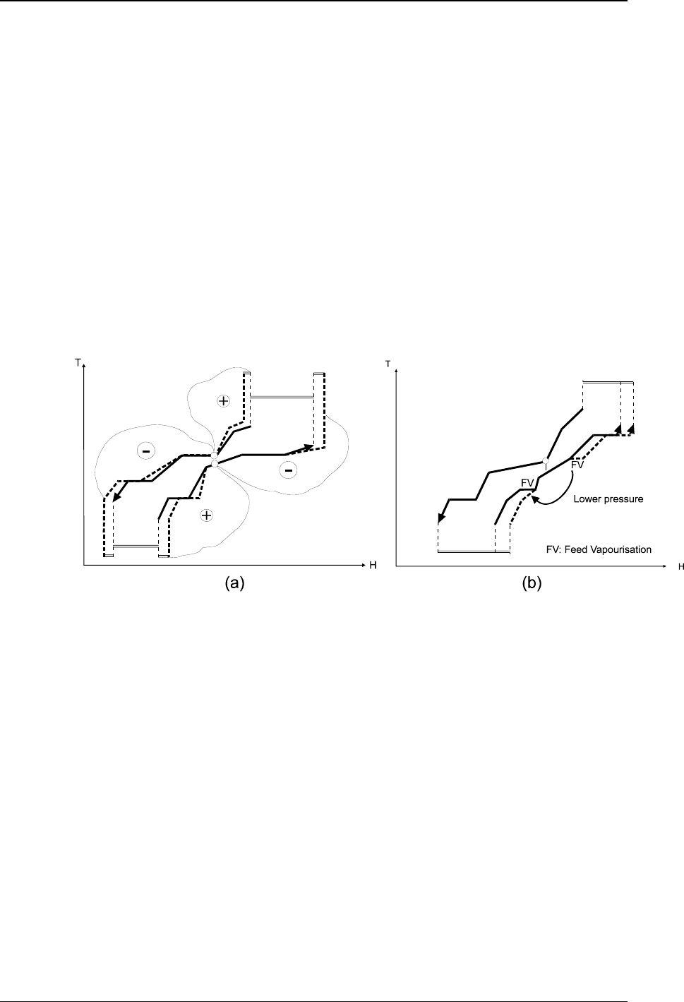
Figure 16: Modifying the process,

(a) The +/- principle for process modifications (b)

Temperature changes can affect the energy targets only if streams are shifted through the

pinch.

Often it is possible to change temperatures rather than heat duties. It is clear from Figure

16(a) that temperature changes that are confined to one side of the pinch will not have any

effect on the energy targets.

Figure 16(b) illustrates how temperature changes across the

pinch can change the energy targets. Due to the reduction in feed vaporisation (FV) pressure,

the feed vaporisation duty has moved from above to below the pinch.

As a result the process

energy target is reduced by the vaporisation duty.

This can be considered as an application of

+/- principle twice.

Thus the beneficial pattern for shifting process temperatures can be summarised as follows:

• Shift hot streams from below the pinch to above the pinch

• Shift cold streams from above the pinch to below the pinch

The +/- principle is in line with the general idea that it ought to be beneficial to increase the

temperature of hot streams (this must make it easier to extract heat from them) and that

Introduction to Pinch Technology

likewise reduce the temperature of the cold streams. Changing the temperature of streams in

this fashion will improve the driving forces in the heat exchanger network but can also

decrease the energy targets if the temperature changes extend across the pinch.

The

designer can predict which modifications would be beneficial, detrimental, or inconsequential

ahead of design.

7.2 Distillation Columns

Distillation columns are one of the major consumers of energy in chemical processes. In this

section the principles for appropriate modification of distillation columns and their integration

with the remaining process are considered. Firstly pinch analysis for stand-alone modification

of distillation columns is considered, followed by principles for appropriate integration of

distillation columns with the remaining process.

The SuperTarget Column module developed by Linnhoff March provides an advanced

software tool for the implementation of standalone column modifications. PinchExpress and

SuperTarget Process provide tools for assessing the impact of column heat integration within

a process.

7.2.1 Stand-alone column modifications

There are several options for improving energy efficiency of distillation columns. These

include reduction in reflux ratio, feed conditioning and side condensing/reboiling etc. Using

pinch analysis it is possible to identify which one of these modifications would be appropriate

for the column and what would be the extent of the modification.

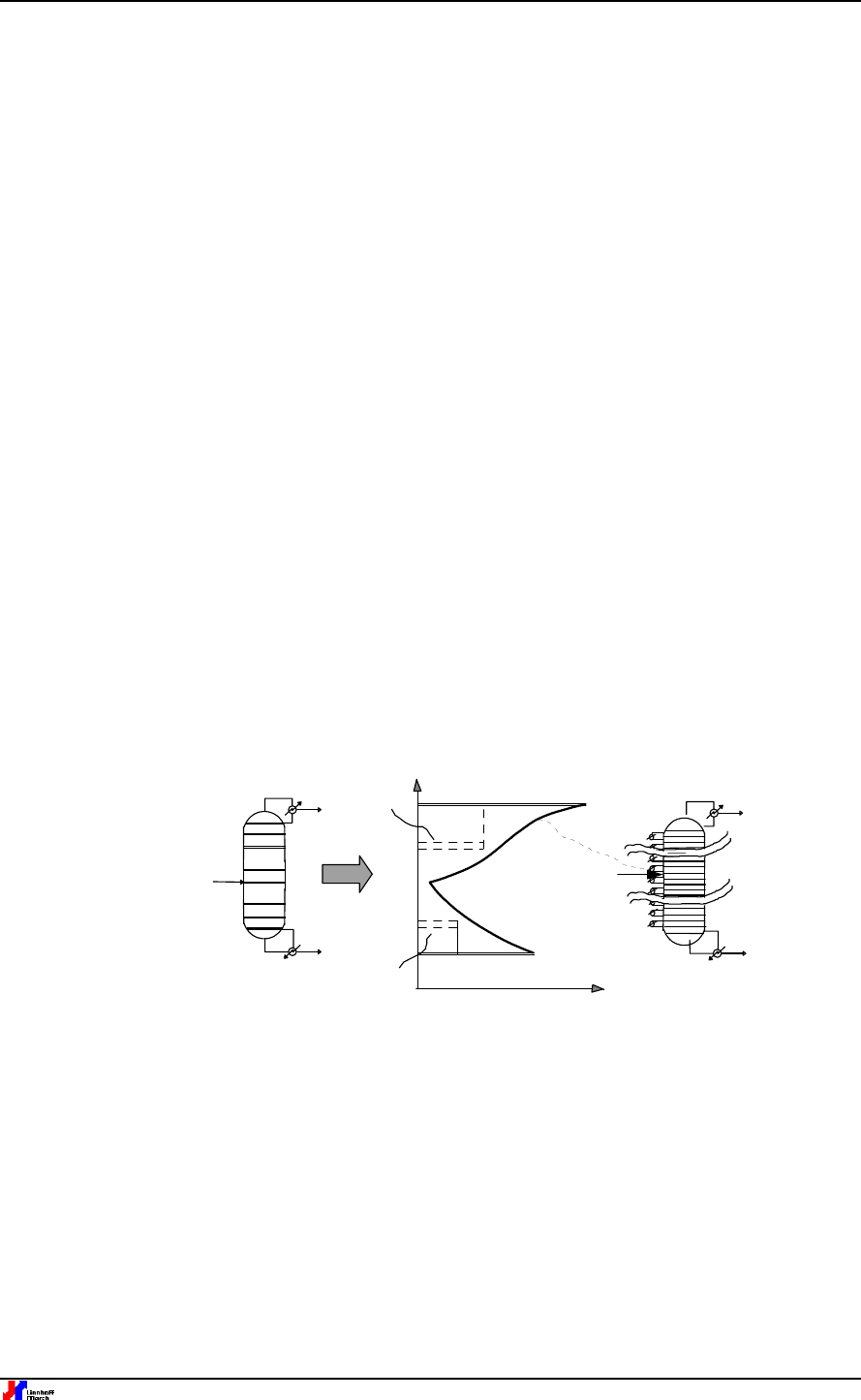
The Column grand composite curve

(a)

Converged

Simulation

Reboiler

Condenser

Column Grand

Composite Curve

(b)

Side

Reboiler

Side

Condenser

(c)

Ideal

Column

Figure 17: Procedure for obtaining Column Grand Composite Curve

The tool that is used for column thermal analysis is called the Column Grand Composite

Curve (CGCC) [15], an example of which is shown in Figure 17.

The procedure for obtaining

the CGCC starts with a converged column simulation as shown in the figure.

From the

simulation, the necessary column information is extracted on a stage-wise basis.

This

information can then processed (for example by using the SuperTarget Column module) to

generate the CGCC as shown in Figure 17(b).

Introduction to Pinch Technology

The CGCC, like the grand composite curve for a process,

provides a thermal profile for a

column and is used for identifying appropriate targets for the column modifications such as

side condensing and reboiling as shown in the figure. In a normal column energy is supplied

to the column at reboiling and condensing temperatures. The CGCC relates to minimum

thermodynamic loss in the column or “Ideal Column” operation (see Figure 17(c)).

For ideal

column operation the column requires infinite number of stages and infinite number of side

reboilers and condensers as shown in Figure 17(c). In this limiting condition, the energy can

be supplied to the column along the temperature profile of the CGCC instead of supplying it at

extreme reboiling and condensing temperatures. The CGCC is plotted in either T-H or Stage-

H dimensions. The pinch point on the CGCC is usually caused by the feed.

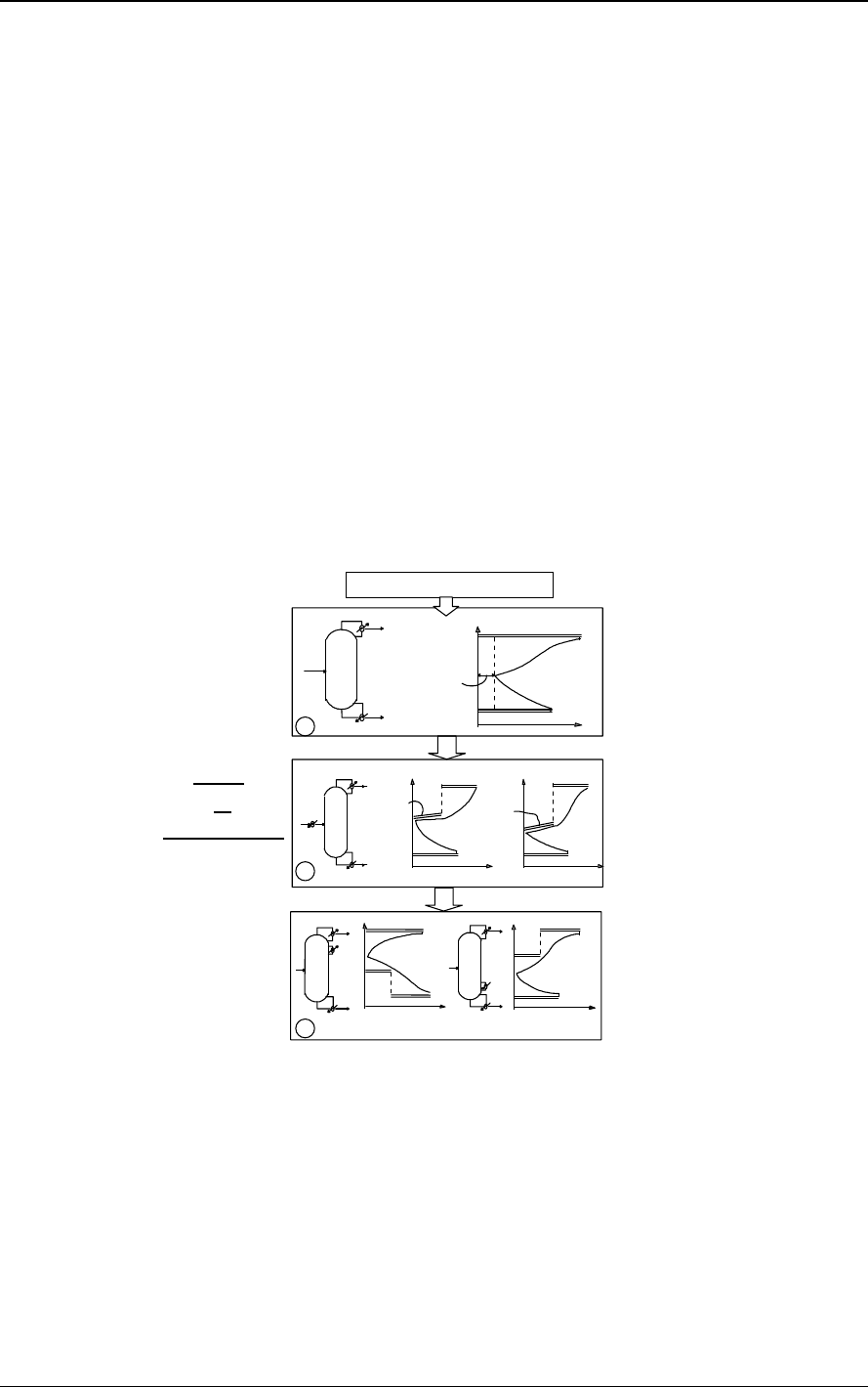
Modifications using the Column grand composite curve

Figure 18 shows the use of the CGCC in identifying appropriate stand-alone column

modifications. Firstly, the feed stage location of the column must be optimised in the

simulation prior to the start of the column thermal analysis. This can be carried out by trying

alternate feed stage locations in simulation and evaluating its impact on the reflux ratio. The

feed stage optimisation is carried out first since it may strongly interact with the other options

for column modifications. The CGCC for the column is then obtained.

Order

Modifications

Reflux

Modification

Feed

Conditioning

Side

Condensing

/Reboiling

Reboiler

Condenser

Scope for

Reflux

Feed Preheat

Temp

Reboiler

Condenser

Reboiler

Side

Temp

Reboiler

Condenser

Stage

Reboiler

Condenser

Scope for

No.

Feed Preheat

Reboiler

Condenser

Temp

Side

Cond.

Feed Stage Optimisation

Figure 18: Using Column Grand Composite Curve to identify column modifications

As shown in Figure 18(a) the horizontal gap between the vertical axis and CGCC pinch point

indicates the scope for reflux improvement in the column. As the reflux ratio is reduced, the

CGCC will move close to the vertical axis. The scope for reflux improvement must be

considered first prior to other thermal modifications since it results in direct heat load savings

both at the reboiler and the condenser level. In an existing column the reflux can be improved

by addition of stages or by improving the efficiency of the existing stages.

After reflux improvement the next priority is to evaluate the scope for feed preheating or

cooling (see Figure 18(b)). This is identified by a “sharp change” in the stage-H CGCC shape

Introduction to Pinch Technology

close to the feed as shown in the figure with a feed preheating example.

The extent of the

sharp change approximately indicates the scope for feed preheating. Successful feed

preheating allows heat load to be shifted from reboiler temperature to the feed preheating

temperature. Analogous procedure applies for feed pre-cooling.

After feed conditioning, side condensing/reboiling should be considered. Figure 18(c)

describes CGCC’s which show potential for side condensing and reboiling. An appropriate

side reboiler allows heat load to be shifted from the reboiling temperature to a side reboiling

temperature without significant reflux penalty.

In general, feed conditioning offers a more moderate temperature level than side

condensing/reboiling. Also feed conditioning is external to the column and is therefore easier

to implement than side condensing and reboiling. The sequence for the different column

modifications can be summarised as follows:

1. Feed stage location

2. Reflux improvement

3. Feed preheating/cooling

4. Side condensing/reboiling.

7.2.2 Column integration

In the previous section, ways of improving column thermal efficiency by stand alone column

modifications were considered. In many situations it is possible to further improve the overall

energy efficiency of the process by appropriate integration of the column with the background

process. By “column integration” a heat exchange link is implied between the column

heating/cooling duties and the process heating/cooling duties or with the utility levels. Figure

19 summarises the principles for appropriate column integration with the background

process.

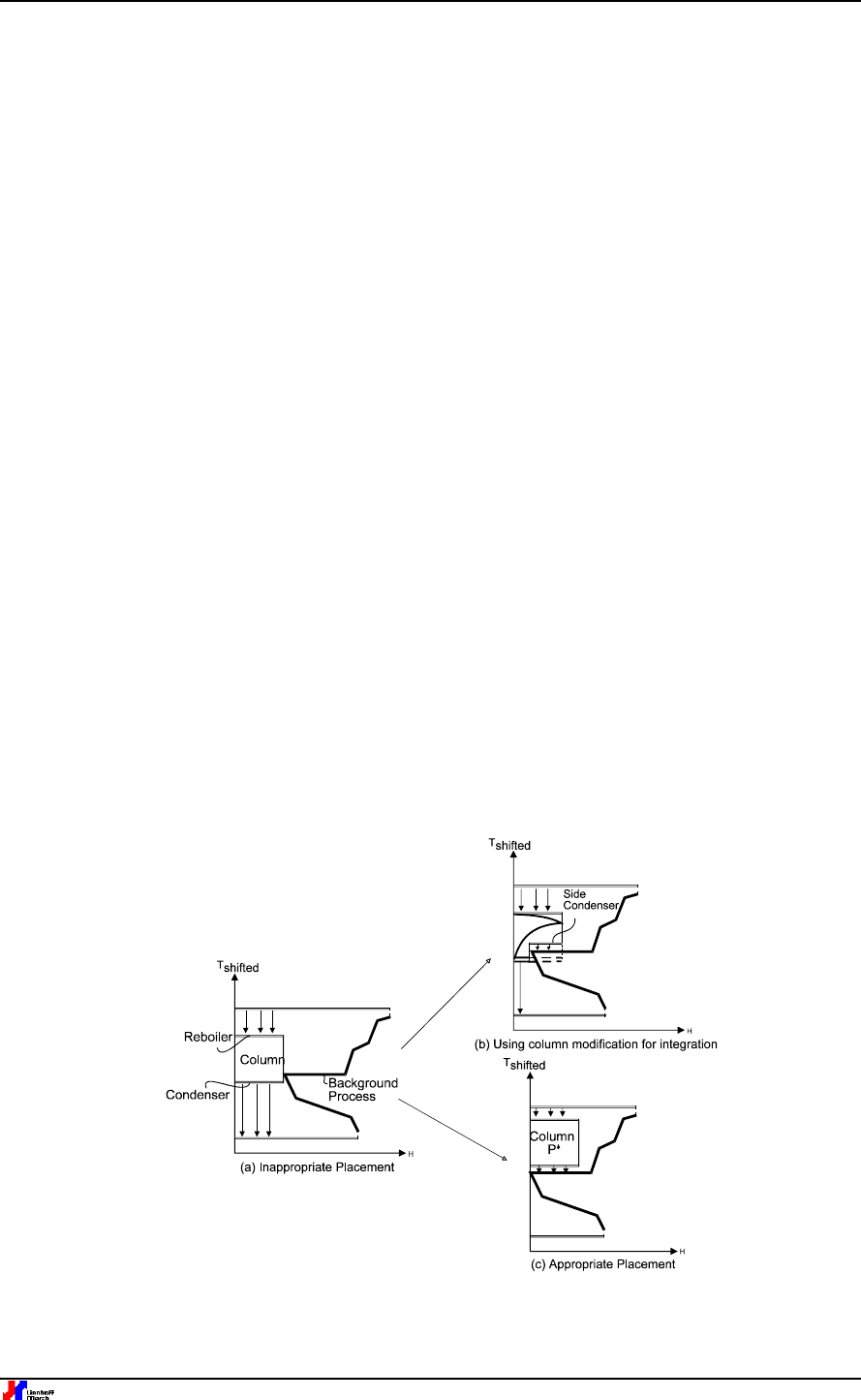
Figure 19: Appropriate Integration of a distillation column with the background process

Introduction to Pinch Technology

Figure 19(a) shows a column with a temperature range across the pinch temperature of the

background process. The background process is represented by its grand composite curve.

The overall energy consumption in this case is equal to that of the column plus the

background process. In other words, there is no benefit in integrating the column with the

background process. The column is therefore inappropriately placed as regards its integration

with the background process.

Figure 19(b) shows the CGCC of the column. The CGCC indicates a potential for side

condensing. The side condenser opens up an opportunity for integration between the column

and the background process. Compared to Figure 19(a) the overall energy consumption

(column + background process) has been reduced due to the integration of the side

condenser.

As an alternative the column pressure could be increased. This will allow a complete

integration between the column and the background process via the column condenser

(Figure 19(c)).

The column is now on one side of the pinch (not across the pinch). The overall

energy consumption (column + background process) equals the energy consumption of the

background process. Energy-wise the column is running effectively for free. The column is

therefore appropriately placed as regards its integration with the background process.

To summarise, the column is inappropriately placed if it is placed across the pinch and has no

potential for integration with the background process via side condensers or reboilers etc.

The integration opportunities are enhanced by stand-alone column modifications such as

feed conditioning and side condensing/reboiling. The column is appropriately placed if it lies

on one side of the pinch and can be accommodated by the grand composite of the

background process.

Appropriate column integration can provide substantial energy benefits. However these

benefits must be compared against associated capital investment and difficulties in operation.

In some cases it is possible to integrate the columns indirectly via the utility system which

may reduce operational difficulties.

The principle of appropriate column integration can also be applied to other thermal

separation equipment such as evaporators [7].

8 Placement of Heat Engines and Heat Pumps

Heat engines and heat pumps constitute key components of the process utility system. In this

section, principles based on pinch analysis for appropriate integration of heat engines and

heat pumps with processes, will be considered.

8.1 Appropriate integration of

heat engines

A heat engine in a process context can have two objectives; supplying for process heat

demand and generation of power. Appropriate integration of heat engines with the process

provides the most energy efficient combination of these objectives. By “integration” here a

heat exchange link is implied between the heat engine and the process. Figure 20 shows

three possibilities of integration of a heat engine with a process. The process is represented

by two regions: one above and other below the pinch. If a heat engine is integrated across the

Introduction to Pinch Technology

pinch (Figure 20(a)), it does not provide any benefit due to integration. The overall energy

consumption is as good as operating the heat engine independent of the process.

Figure 20: Appropriate Placement Principle for heat engines

If the heat engine is placed so that it rejects heat into the process above the pinch

temperature (Figure 20(b)), it transfers the heat to process heat sink, thereby reducing the hot

utility demand. Due to the heat engine the overall hot utility requirement is only increased by

W (i.e. the shaftwork). This implies a 100% efficient heat engine. The heat engine is therefore

appropriately placed.

If the heat engine is placed so that it takes in energy from the process below the pinch

temperature (Figure 20(c)), it takes that energy from an overall process heat source. Here the

engine runs on process heat free of fuel cost and reduces the overall cold utility requirement

by W. The heat engine is again appropriately placed.

To summarise, appropriate placement of heat engines is either above the pinch or below the

pinch but not across the pinch.

The above mentioned principle provides basic rules for integration of heat engines. The rules

assume that the process is able to absorb all the heat rejected by the heat engine. The

designers therefore must use the grand composite curve in setting the integration of the heat

engine with the process.

8.1.1 Identifying opportunities for heat engine placement

Figure 21 shows the placement of steam and gas turbines against the grand composite

curve.

Both the placements are on one side of the pinch and are therefore appropriate. Figure

21(a) shows the integration of a steam turbine system with a process. Starting from the

targets for steam demands (A and B) the key parameters for the steam turbine system are

set. For a given boiler steam pressure, the overall fuel demand and shaftwork (W) can be

calculated. The overall fuel demand = A+B+W+Q

LOSS

where Q

LOSS

is the heat loss from the

boiler.

Thus targets are set for the overall fuel demand and shaftwork potential for the process

starting from the grand composite curve.

Introduction to Pinch Technology

Figure 21: Placement of steam and gas turbines against the grand composite curve

Figure 21(b) shows an example of appropriate integration of gas turbine with the process.

The

exhaust heat of the gas turbine is utilised for satisfying process heating demand.

This is

represented by placement of thermal profile of the exhaust heat against the grand composite

curve as shown in the figure.

The gas turbine exhaust heat therefore saves the equivalent hot

utility demand of the process.

The heat from the gas turbine fuel demand is obtained by the

sum of process heating demand (A), shaftwork (W) and the heat loss below the pinch

temperature (Q

LOSS

8.2 Appropriate integration of heat pumps

A heat pump accepts heat at a lower temperature and, by using mechanical power, rejects

the heat at a higher temperature.

The rejected heat is then the sum of the input heat and the

mechanical power.

Heat pumps provide a way of using waste heat for useful process heating.

The pinch analysis principle for integration of heat pumps is useful in setting key design

parameters for the heat pumps.

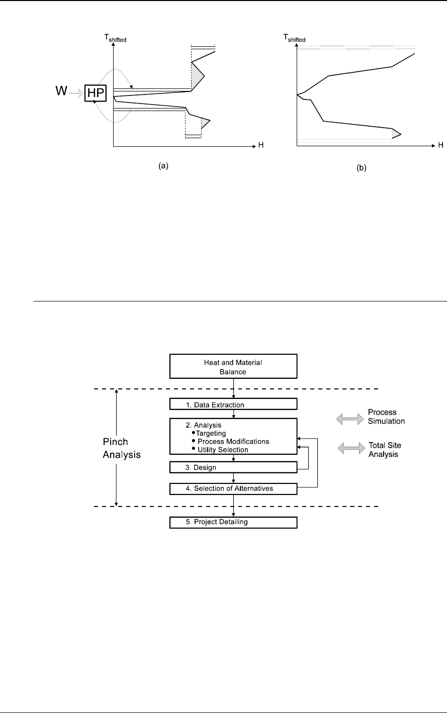
Figure 22 shows the three arrangements that a heat pump may take relative to the pinch.

First, heat can be taken from above the pinch and rejected at a higher temperature also

above the pinch (Figure 22(a)).

This saves hot utility by the amount W but only at the expense

of an equal input of power W.

Because power is much more expensive than heat (typically 4

to 5 times), this is not an efficient solution.

Introduction to Pinch Technology

Inappropriate placement

(a)

Inappropriate placement

(b)

Appropriate placement

(c)

Figure 22: Placement of heat pumps.

Second, the heat pump can take in heat from below the pinch and reject it at a higher

temperature, also below the pinch (Figure 22(b)).

This is even more inefficient because W

units of heat (from power) is rejected to a part of the process that already had an excess of

heat (remember, the process below the pinch is a heat source).

The third option is to take in

heat from below the pinch and reject it at a temperature above the pinch (Figure 22(c)).

This

provides savings in both hot and cold utilities because it is pumping heat from a source

(below the pinch) to a sink (above the pinch).

The appropriate way to integrate a heat pump is

therefore across the pinch.

It is important to note here that “pinch” denotes process as well as

utility pinch. The overall economics of the heat pump however, depend on the heat savings

due to heat pump compared with the cost of power input and capital cost of the heat pump

and associated heat exchangers.

8.2.1 Identifying opportunities for heat pump placement

As discussed previously, the economics of the heat pump placement depend on the balance

between process heat savings versus power requirement for heat pumping. In order to make

the heat pump option economical a large process heat duty and small temperature differential

across the heat pump are needed. By examining the grand composite curve of a process, it is

possible to identify quickly when opportunities for introducing a heat pump may exist.

Consider Figure 23(a). The grand composite curve shows a region of small temperature

change and large enthalpy change above and below the pinch.

This pointed “nose” at the

pinch indicates that a heat pump can be installed across the small temperature change for a

relatively large saving in heating and cooling demand.

The energy saving will therefore be

high for a relatively small expense in power (high coefficient of performance).

The diagram in

Figure 23(b), however, shows that the heat pump option may be uneconomical since the

temperature differential across the heat pump is quite large which will result in high power

requirement for the heat pump.

Introduction to Pinch Technology

Figure 23: A pointed ‘nose’ at the process or utility pinch indicates a good heat pump

opportunity.

Refrigeration systems constitute another class of heat pumping applicable to sub-ambient

temperature regions. The principles of appropriate placement as discussed in this section are

also applicable to refrigeration systems. In addition techniques have been developed which

provide a more detailed approach for the placement of refrigeration levels against the grand

composite curve [11, 12].

9 Heat Exchanger Network Design

The figure below provides an overview of key steps in pinch technology.

Figure 24: Key steps in Pinch Technology

So far the first two steps have been considered, namely, data extraction and analysis. Data

extraction involves translation of flow-sheet information into relevant thermal and cost

information required for the application of pinch technology (section 3). For more information

on the principles of converting flowsheet data to pinch analysis data see "Data Extraction

Principles" (in section 10). The second step in pinch technology is pinch analysis based on

targets. This involves targeting for energy (section 4), trade-offs in targeting mode between

capital and energy (section 6), targeting for process modifications (section 7) and targeting for

multiple utility levels (section 5) and placement of heat engines and heat pumps (section 8).

Introduction to Pinch Technology

In the analysis stage the objective is to explore various options for process improvement

quickly and easily using targeting, without getting into the detail of specific flow-sheet

changes. This allows quick screening of various options for process improvement such as

energy recovery, process modifications, utility system integration etc. The key improvement

options identified in the analysis stage need to be implemented in design. In this section the

focus is on the design aspect of pinch technology. This translates the ideas for improvement

obtained during the analysis/targeting stage into specific modifications of the heat exchanger

network.

The heat exchanger network design procedure is based upon pinch analysis principles and is

called the Pinch Design Method. The method systematically leads the engineer to good

network designs that achieve the energy targets within practical limits. The network design

procedure uses a special representation for heat exchanger networks called the “Grid

Diagram” (section 9.2). The network design procedures for new design and retrofit design are

discussed separately in sections 9.3 and 9.4 respectively. Before this however, some further

consideration is given to network representation.

9.1 The Difference Between Streams and Branches

Previous sections have described how Pinch Technology uses stream data and utility data to

represent a process design. This representation is sufficient for targeting, which only needs to

know about the heat sources and sinks at each temperature interval. It is not complete

enough, however, to represent a network of heat exchanger matches because it does not

contain any information on stream splits and mixers. An additional structure must therefore be

overlaid on top of the stream and utility data. The features of this additional representation

used in PinchExpress are as follows:

• A stream or utility is split into a number of branches. Initially, each stream has only one

branch. More are created, however, as splits and mixers are placed on the stream.

• The first branch on a stream either ends at a split or goes to the end of the stream.

• New branches are created each side of a split or mix. A branch never continues through

a split or mix.

• Branches do, however, continue straight through heat exchangers matches. A branch

never divides at a match.

• Each branch has the following data associated with it:

TS: The source temperature of the branch. For a branch at the start of a stream this

is the same as the stream TS. For others, it is the temperature out of the split or mix.

TT: The target temperature of the branch. For a branch at the end of a stream this is

the same as the stream TT. For others, it is the temperature into the split or mix.

FF: The flow fraction of the branch, relative to the original stream. This is determined

by the upstream splits and mixers.

Number: The branch number. In PinchExpress, this is created automatically and

cannot be changed.

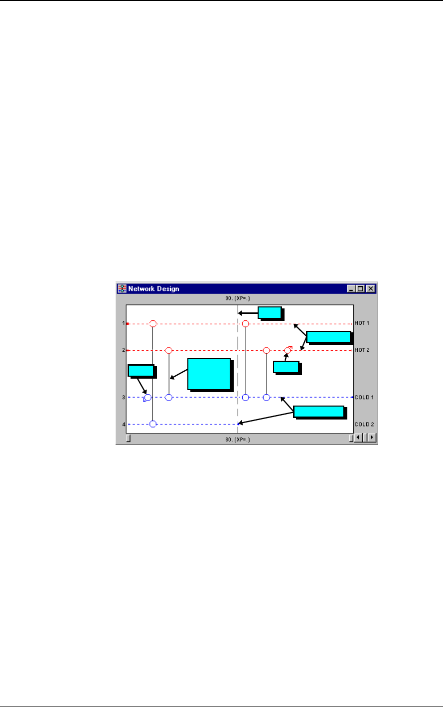
Introduction to Pinch Technology

Name: The branch name. This is generated automatically by PinchExpress but can,

in most cases, be changed. The first branch on a stream has the same name as the

stream.

• At any temperature the Mass Flow Heat Capacity of a branch is defined as follows:

Branch CP = FF * Stream CP at the same temperature

• The branch structure does not change the basic stream data. Changes in the stream

duties continue to affect the branch duties and CPs.

• All the branches into a mix must belong to the same stream. Mixers between streams are

NOT allowed.

• A branch cannot mix back in upstream of its starting point. Stream loops such as this are

NOT allowed.

9.2 The Grid Diagram for heat exchanger network representation

Figure 25 shows the Grid Diagram representation of a heat exchanger network.

Hot Streams

Cooler

Cold Streams

Heater

Pinch

Process to

Process

Exchanger

Figure 25: The Grid diagram for easier representation of the heat exchanger network

The hot streams are shown at the top of the figure, running from left to right.

Cold streams run

across the bottom, from right to left.

A heat exchanger transferring heat between the process

streams is shown by a vertical line joining circles on the two matched streams.

A heater is

shown as a single blue circle with an arrow pointing down and a cooler is shown as a single

red circle with an arrow pointing up.

The pinch principle, discussed in sub-section 4.3, explains how the process must be

separated into two regions, above and below the pinch, for network design in order to achieve

the energy targets.

The understanding of the pinch location is therefore very important for

network design.

In the grid diagram the process pinch location is shown by a dashed vertical line cutting the

process into two parts. The pinch hot and cold temperatures as determined from the

composite curves are shown on the grid diagram (shown as 90ºC and 80ºC respectively in

Figure 25).

The difference between the hot and cold pinch temperatures equals DT

min

as seen

on the composite curves. The process below the pinch (heat source) is shown on the right

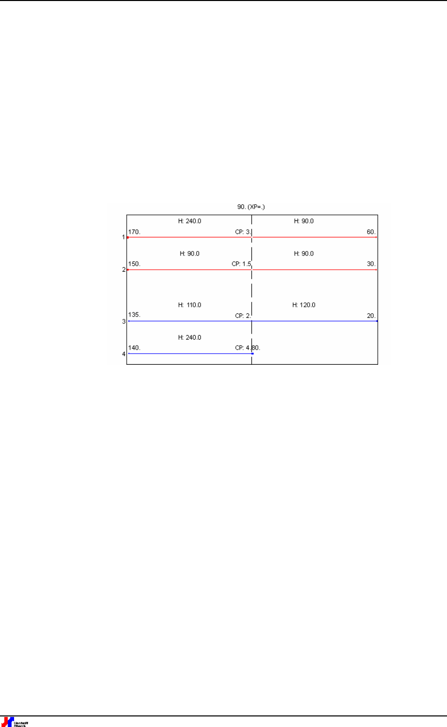
Introduction to Pinch Technology

whilst the process above the pinch (heat sink) is shown on the left. From this it can be seen

that the horizontal axis implies a temperature decrease from left to right. However, it is

important to note that this is not a gradual scale. Instead, the grid diagram just shows

significant temperature locations, such as whether a stream starts above or below a pinch.

Applying the three rules of the pinch principle therefore means that there must be no heater

on the right hand section of the grid diagram, no cooler on the left hand section and no

process heat exchangers between the hot streams on the left hand section and the cold

streams on the right hand section. This will ensure that the network will always achieve the

energy target.

9.3 The New Design Method

Figure 26: Grid diagram for the example problem

Here, the pinch design method [2, 3] is illustrated, using the example problem shown earlier

in Figure 2. The grid diagram for this process is shown in Figure 26. The three rules of the

pinch principle (section 4.3) are central to the procedure for designing the network. According to

the Pinch rules there must be no external cooling above the pinch (on the left side of the grid

diagram) so hot streams on this side must be brought to pinch temperature by heat transfer with

cold streams on the same side i.e. on the left. Similarly, cold streams on the right hand side of the

grid diagram must be brought up to the pinch temperature using hot streams on the right rather

than utility heating. The DT

min

puts another constraint on the design because it has been defined

as the minimum temperature difference for heat transfer anywhere in the system.

9.3.1 Design Above The Pinch

Some ground rules for setting up the heat exchanger matches between the hot and the cold

streams on each side of the pinch (Figure 27) are now considered. Take the example

streams shown in Figure 27(a). A proposed match can be drawn between streams 1 and 3. A

temperature-enthalpy diagram of the proposed match is shown in the inset. Note that the

stream directions previously shown on temperature-enthalpy plots have been reversed so

that they can be more easily related to the grid diagram. Because the CP of stream 3 is less

than stream 1 (CP of cold stream less than CP of hot stream), as soon as a heat load is

applied, the temperatures of the two streams converge to closer than DT

min

. This means that

the proposed heat exchanger is not feasible and another match must be found.

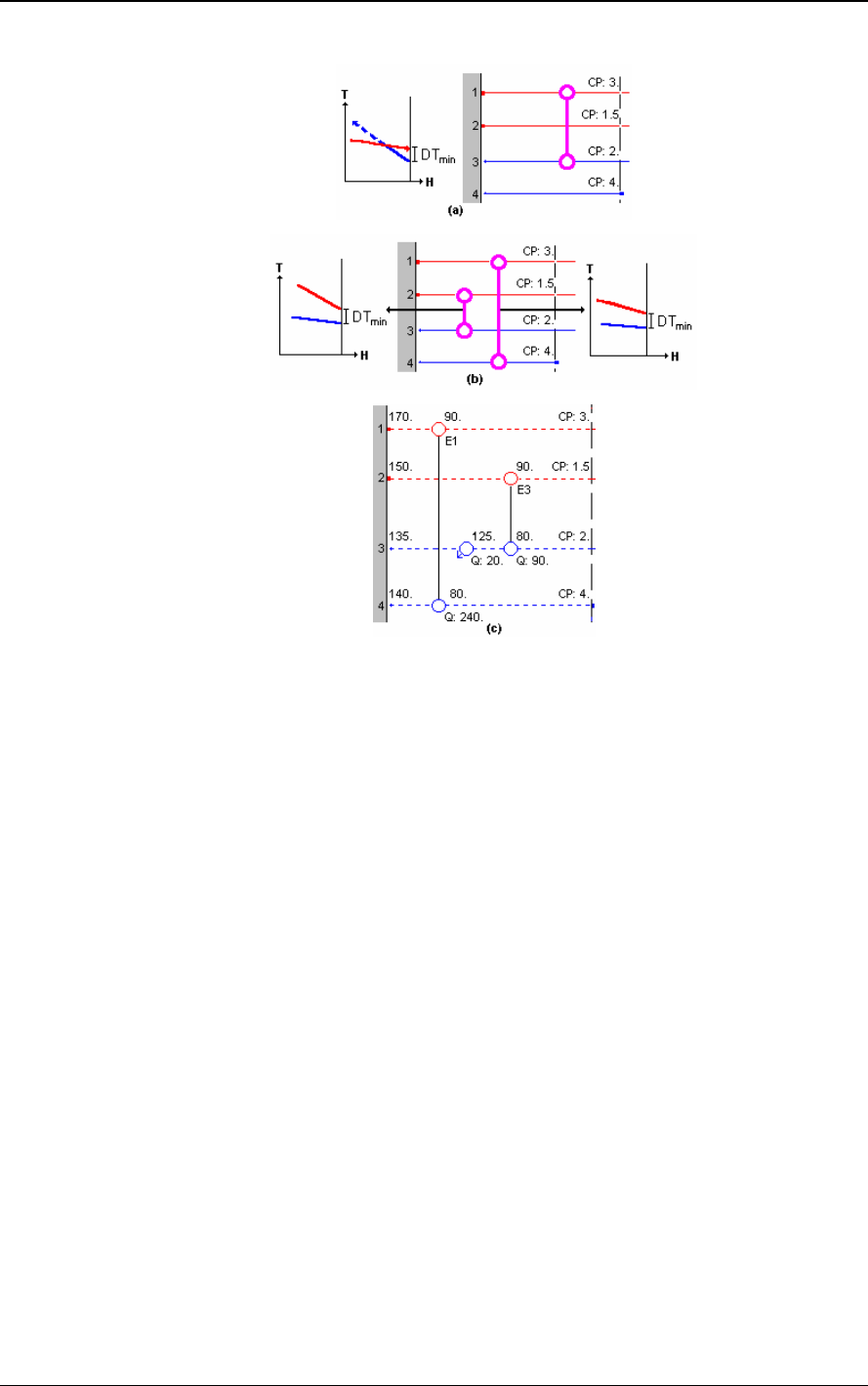
Introduction to Pinch Technology

Figure 27: Criteria for temperature feasibility at the pinch

In Figure 27(b), streams 1 and 4 are matched. In this case the CP of stream 4 is greater than

the CP of stream 1 (CP of cold stream greater than CP of hot stream). The relative gradients

on the temperature-enthalpy plot means that the streams diverge from DT

min

; the match is

feasible. For the temperature feasibility of the matches close to the pinch, the CP of the

streams going out of the pinch needs to be greater than the CP of the stream coming into the

pinch. Thus for temperature feasibility there is a "CP rule":

out

≥ CP

Stream 2 also has to be brought to the pinch temperature and this is achieved using a match

with stream 3. Since the CP of stream 3 (stream going out) is greater than the CP of stream 2

(stream going in), the temperature-enthalpy plot is again divergent (see the other inset on

27(b)) and the match is feasible. Now that both the hot streams on the left side of the pinch

are completely matched with the cold streams, the possibility of using cooling utility above the

pinch has been eliminated. The remaining heating load on the cold streams must now be

provided by the utilities.

Since stream 1 requires 240 kW of cooling and stream 4 needs 240 kW of heating on the left

side of the pinch, the 1-4 match satisfies the requirements of both the streams. But the 2-3

match can only satisfy stream 2 since stream 2 can only give up 90 kW of heat before it

reaches the pinch temperature. This will heat stream 3 to 125ºC but the target temperature is

135ºC. An extra 20 kW must be provided by utilities to satisfy the heating requirements of

stream 3. This is indeed the minimum utility requirement for the network (at DT

min

= 10ºC).

Figure 27(c) shows the completed design for the section to the left of the pinch.

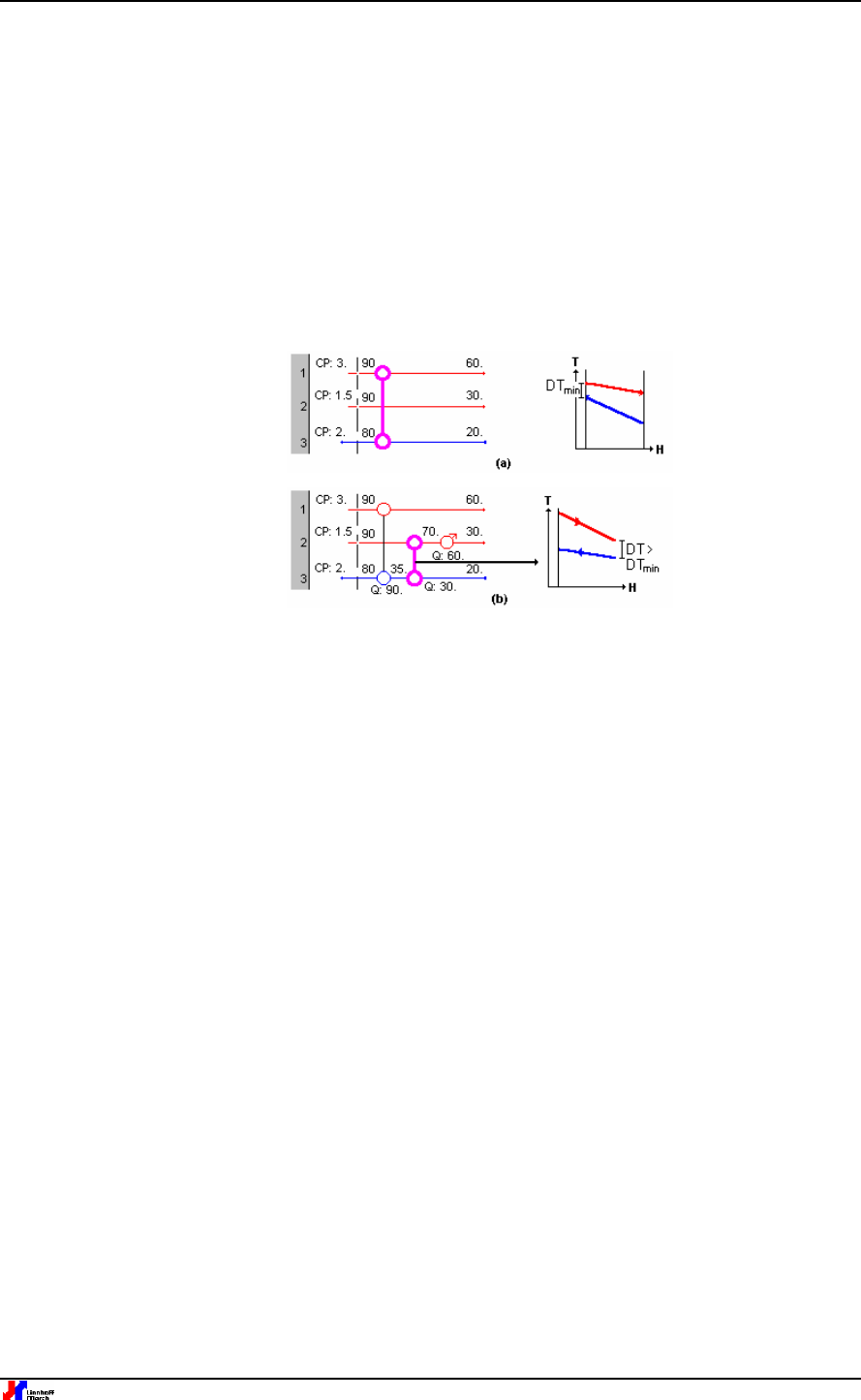
Introduction to Pinch Technology

PinchExpress gives a lot of help with this task because of a powerful feature called

"Automatic Remaining Problem Analysis". This means that every time a change is made, it

can instantly be seen if that change will lead to an energy penalty in the finished design.

9.3.2 Design Below The Pinch

Figure 28 shows the equivalent design below the pinch (on the right of the grid). The rule

below the pinch is not to use utility heating so streams 1 and 3 are matched. The inset shows

that the match is feasible since the CP of stream 1 (the stream going out of the pinch) is

greater than the CP of stream 3 (the stream going into the pinch). As expected, the

temperature-enthalpy plots diverge as they leave the pinch.

Figure 28: Network design below the pinch

It is important to realise that the "CP rule" for temperature feasibility is only rigid for units

directly adjacent to the pinch. In the example, Figure 28(b) shows that the proposed match

between streams 2 and 3 displays converging temperatures on the temperature-enthalpy

plot. However, since the match is not adjacent to the pinch, it does not have to bring the

streams to the pinch temperature difference. This means that, even though the temperatures

converge, they do not necessarily end up at a temperature difference smaller than DT

min

. In

this instance, the final DT is greater than DT

min

and the match is still feasible.

Figure 28(b) shows the completed design to the right of the pinch. Putting a heat load of 30

kW on the 2-3 match (all the cooling that stream 3 can provide before it reaches its target

temperature) means that residual cooling of 60 kW must be provided to stream 2 by utilities.

9.3.3 Completed Minimum Energy Requirement Design

The overall network resulting from the above and below pinch designs is shown in Figure 29

and is known as a minimum energy requirement (MER) design since it meets the minimum

energy target.

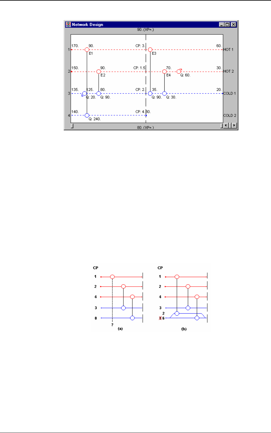
Introduction to Pinch Technology

Figure 29: Completed MER network design based on pinch design method

PinchExpress has the facility for “on-screen” network design using the pinch design method.

This includes a comprehensive set of tools for recalculating portions of the network and

analysing how well the current design compares to the target.

9.3.4 Stream splitting in network design

For the region around the pinch, there is a problem if there are more streams going into the pinch

than there are coming out. Consider for example a grid representation on the left side of the pinch

as shown in Figure 30(a). According to the rules, each stream going into the pinch needs to be

matched with an outgoing stream to bring it to the pinch temperature. Therefore it is required to

split the outgoing streams to equal the total number to that of the streams going into the pinch. In

Figure 30(a) the number of streams going into the pinch is 3 while the number of outgoing

streams is 2. A split of an outgoing stream is necessary, as shown in Figure 30(b). The splitting

should also ensure that the CP rule is not violated.

Figure 30: Criteria for stream splitting at the pinch based on number of streams at the pinch

There is also a problem if there are matches at the pinch that do not comply with the CP

out

= CP

rule. In this case, an incoming stream could be split to reduce its CP. Consider the example

shown in Figure 31(a). One of the solutions is to split the incoming stream with CP of 10 (see

Figure 31(b)). This network design requires only one split and it achieves the minimum energy

requirement as well as the temperature feasibility. One of the objectives in network design is to

minimise the number of stream splits. Stream splitting is explained in more detail in reference [2,

3].

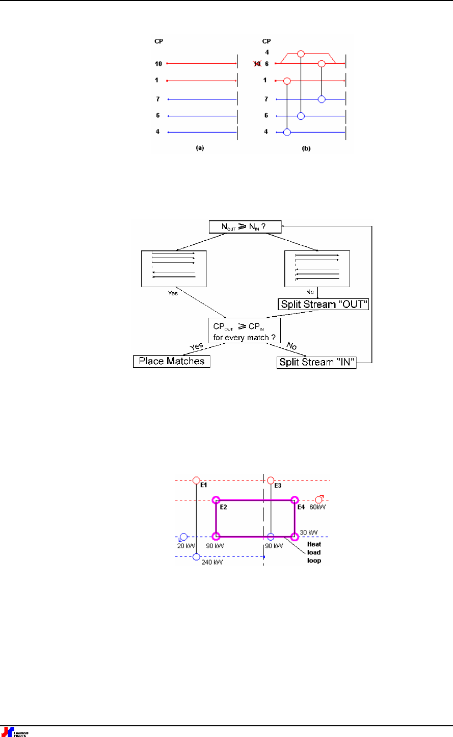
Introduction to Pinch Technology

Figure 31: Incoming stream split to comply with CP

out

= CP

rule.

Figure 32 summarises the rules for stream splitting during network design. N

and N

OUT

are

the number of streams coming in and going out of the pinch respectively.

Figure 32: A summary of stream splitting procedure during network design

9.3.5 Network evolution: Heat load loops and heat load paths

After the network has been designed according to the pinch design rules it can be subjected to

further simplification and capital-energy optimisation. The figures below illustrate the degrees of

freedom available for network evolution after the pinch design method.

Figure 33: A heat load loop

Figure 33 shows a degree of freedom called the “Heat Load Loop” [2, 3]. The loop is shown by

the solid line marking a circuit between matches 2 and 4. Heat duties can be shifted around a

loop without affecting the heat duties imposed on other units in the network which are not part of

the loop. This may result in reducing the heat load on a unit to zero (e.g. exchanger 4). However

such a change will affect the temperature driving forces in the network. The temperature driving

force will become less than DT

min

and in some cases it may result in temperature infeasibilty. The

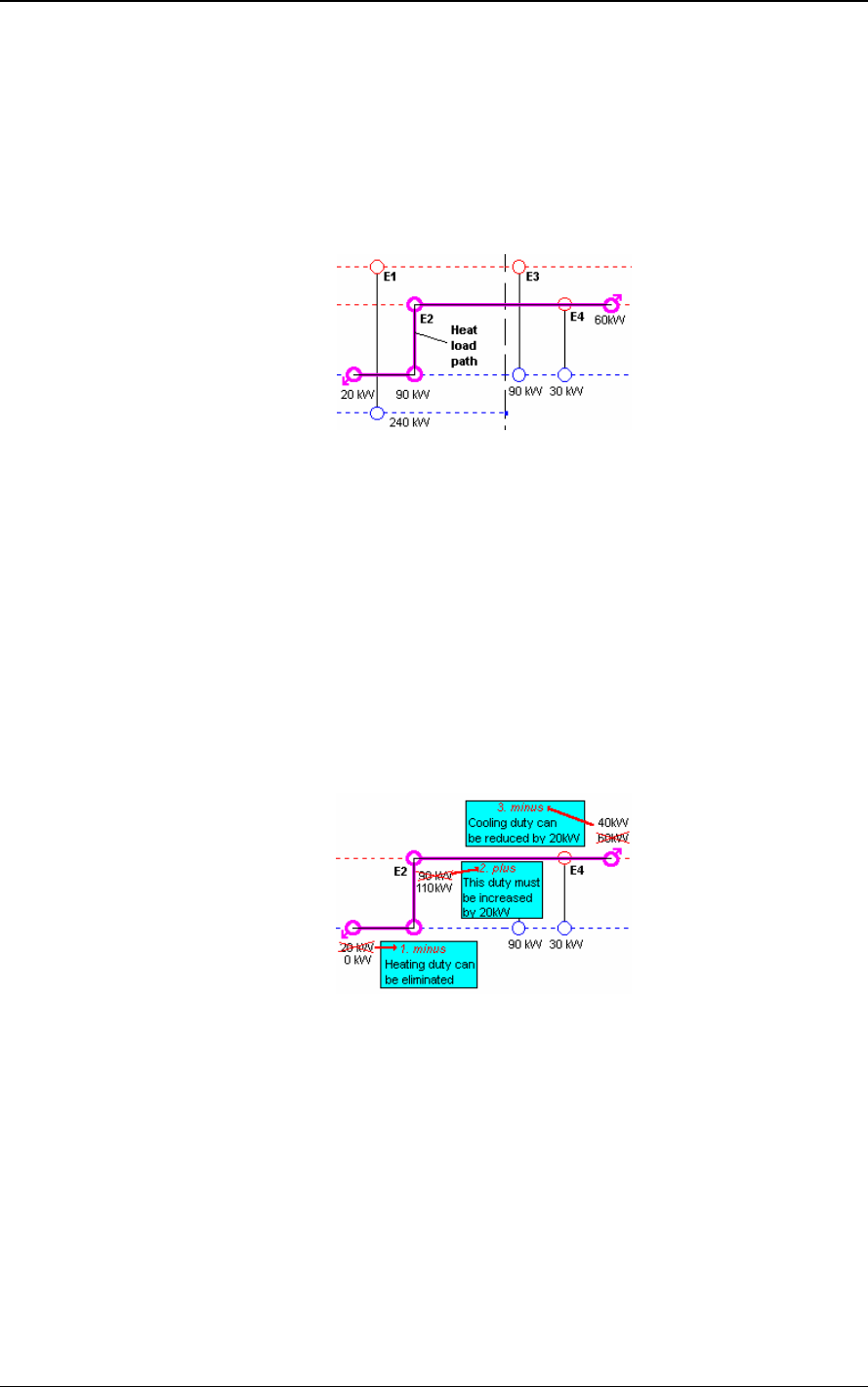
Introduction to Pinch Technology

cost saving in installation of a unit needs to be compared with increase in the surface area due to

the reduction in temperature difference.

Such an optimisation can be carried out in the SuperTarget Process Module developed by

Linnhoff March. PinchExpress can also be used to shift heat loads around loops. In many

situations using heat load loops can reduce both the number of exchanger units and the overall

network cost.

Figure 34: A heat load path

Figure 34 illustrates the second degree of freedom for network evolution called the "Heat

Load Path” [2, 3]. A path provides a continuous connection between two utilities and therefore

allows the transfer of heat loads between heat exchanger units and the utilities. In Figure 34

the path connects heater, exchangers 2, 4 and the cooler. By changing the heat loads of

exchangers 2 or 4, the heater and cooler heat loads will change by the same amount but in

an opposite manner. This is demonstrated below in Figure 35. The heating duty can be

eliminated if the duty on exchanger 2 is increased by the corresponding amount. Then the

cooling duty must also be decreased by this amount to maintain the energy balance on the

hot stream. Heat load paths exploit capital-energy trade-off in specific parts of the network.

SuperTarget Process and PinchExpress also have the facility to optimise the network

performance using heat load paths.

Figure 35: Using a path to reduce utility use

Heat load loops and paths provide additional degrees of freedom for the designer in order to

further simplify the network or reduce the overall network cost.

9.3.6 Network design for multiple utilities

The example for network design as demonstrated previously uses one hot and one cold

utility. For processes involving multiple utilities, all the utilities are incorporated in the grid

diagram as streams. The network is therefore “balanced” in enthalpy terms. The grid diagram

also incorporates all the utility as well as process pinches.

The network design for multiple utilities is more complex due to the occurrence of multiple

pinches in the problem. References [2, 3] are appropriate for further background on network

Introduction to Pinch Technology

design involving multiple utilities. PinchExpress incorporates features for the placement of

multiple utilities.

9.3.7 Summary: New heat exchanger network design

The steps to be followed in network design for a grass roots project can be summarised as

follows:

a) Develop a Minimum Energy Requirement (MER) network

• Divide problem at the Pinch

• Start at the pinch and move away

• Start with biggest stream “IN”

• Observe CP

OUT

≥ CP

, splitting streams where necessary

• Place all pinch matches first

• Maximise loads on all pinch matches to minimise number of units (the "tick-off" rule)

• Fill in the rest

• Merge above and below the pinch designs

b) Evolve the MER network for network simplicity and capital-energy trade-off

• Exploit heat load loops and heat load paths

• Optimise network performance using advanced tools in SuperTarget Process

9.4 Heat Exchanger Network Design for Retrofits

PinchExpress provides the necessary tools for retrofit design using one of the three methods.

1. Pinch Design Method with maximum re-use of existing exchangers

2. Correction of Cross-Pinch Exchangers

3. Analysis of Exchanger Paths

The retrofit design methods are illustrated using screen shots from Linnhoff March’s

PinchExpress package.

Which Retrofit Method is Suitable?

The first step in retrofit design is to decide which retrofit method is most suitable for the

project. The hierarchical diagram shown in Figure 36 indicates when each of the three

methods is suitable. Detailed explanation of the methods is provided below .

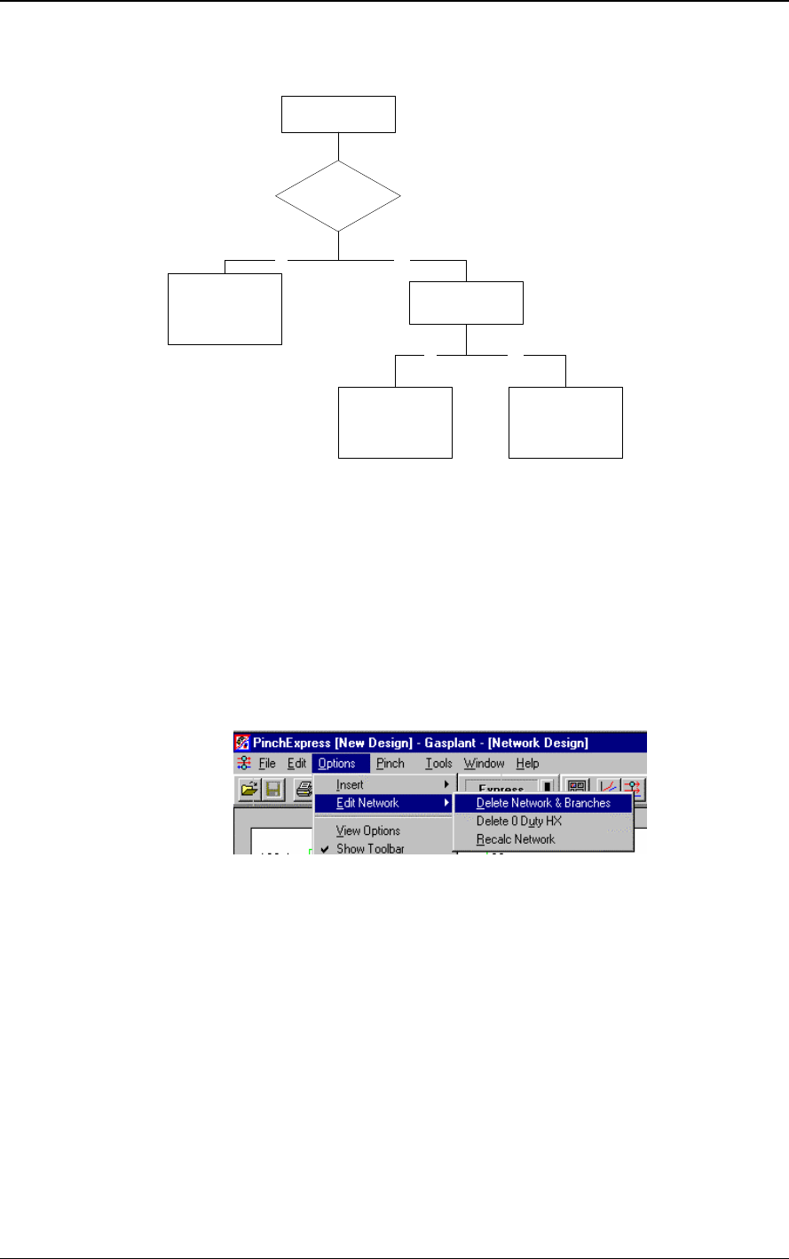
Introduction to Pinch Technology

Retrofit project with

large scope for savings

Is the current heat

integration significant?

Pinch Design Method

Re-use existing

exchangers

Cross-Pinch

Analysis

Path Analysis

No Yes

Are composite curves

parallel with little use of

intermediate utilities?

Figure 36: Hierarchy of retrofit design

9.4.1 Pinch Design Method with maximum re-use of existing exchangers

This method has been described in the previous section for design from grassroots. The

method is briefly described for retrofits as:

a) Delete the existing network as shown in Figure 37

b) Re-design the network by following the Pinch Design Method as detailed on page 33

c) Re-use existing exchangers in place of new ones between the same streams

Figure 37: Delete existing network before applying the pinch Design Method

9.4.2 Correcting Cross-Pinch Exchangers

In situations where the existing network already involves many process-process heat

exchangers, it is not appropriate to delete the entire network in order to apply the Pinch

Design Method. Instead, it is better to apply a method that makes incremental changes to the

existing network, with a corresponding quantification of the benefits.

This is particularly true of processes with diverging composite curves and significant use of

intermediate utilities. Indeed, for such a process it is usually possible to discover a series of

independent retrofit projects, each involving just a few modifications to the network. It is then

possible to rank these projects and just choose the best ones according to some practical or

economic criteria.

The method is described in the following flowchart:

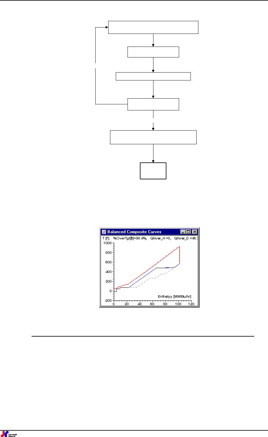
Introduction to Pinch Technology

Use cross-pinch analysis to find a promising project in

the current network

Use the Grid Diagram to

design the project

Record the savings achieved by this project

Are there any significant

savings left?

Finished

Yes

Rank the projects according to the savings

achieved, the number of modifications required etc.

Figure 38: Procedure for correcting cross-pinch exchangers

An Ammonia Synthesis example will be used to explain the steps involved in this method.

The Balanced Composite Curves for this example (Figure 39) show a scope for saving of

98.4% with a significant use of intermediate utilities.

Figure 39: Example for retrofit design using Cross-Pinch Analysis

Use cross-pinch analysis to find a promising project in the current network

1. From the ‘Pinches’ report of the potential savings window, identify the pinch region with

the largest monetary savings potential and note the corresponding pinch temperature,

Figure 40.

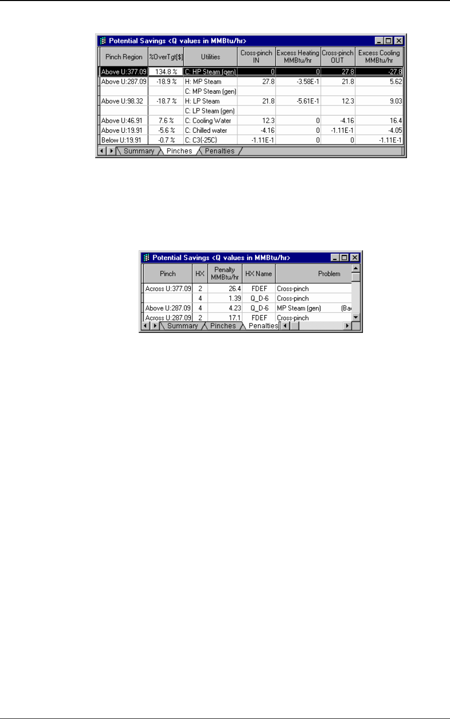
Introduction to Pinch Technology

Figure 40: Pinches report indicate that the most significant pinch region is U:377.09 (HP-

Steam (gen))

2. From the ‘Penalties’ report of the potential savings window, identify the exchanger with

the largest cross-pinch duty in this region (see Figure 41). Alternatively, use the Energy

Penalties graph for the same purpose..

Figure 41: The largest penalty at U:377.09 is exchanger FDEF

3. Determine what will be required to correct the cross-pinch. The options are as follows:

a) Reduce the duty of the exchanger, or delete it altogether. This can be tested by simply

editing the exchanger and seeing if there is a benefit (according to the Summary

report of the potential savings window). Save the data file first, so that you can undo

the change if necessary by reloading the file.

If this approach is used on a complete network then the reported savings can be

achieved by simply replacing the duty with appropriate heaters and coolers. In other

cases, there may be a need for additional heat exchange with the previously

unmatched streams.

b) Move one end of the exchanger to a different utility. This can be done by simply

dragging the end of the match with the mouse. Again, the Summary report will

immediately show any benefit

c) Look for projects involving two or more exchangers. For example, remove the cross-

pinch by changing one of the inlet temperatures rather than reducing the duty.

However, to do this you must compensate by a corresponding change to adjacent

exchangers, heaters or coolers.

As with option (a), you can test the benefit of changing several matches by deleting them

together and observing the reported savings. Again, save the data file first, so that you

can undo the change by just reloading the file.

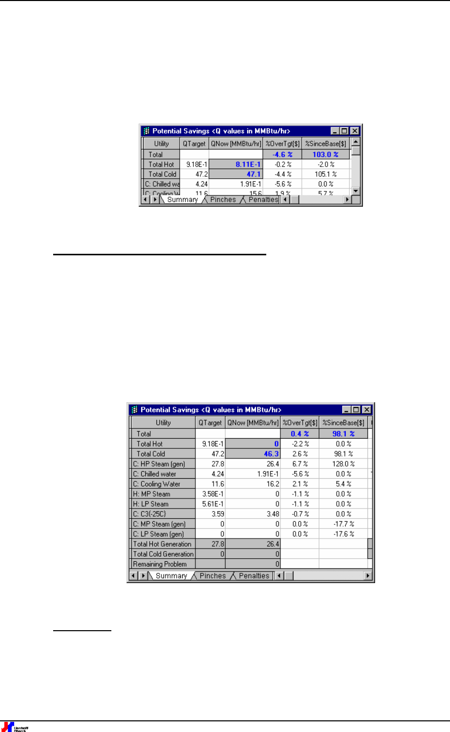
Introduction to Pinch Technology

In the example, virtually all of the savings can be achieved by removing the cross-pinch in

exchanger “FDEF”. This is done by decreasing the hot inlet temperature to FDEF and

reducing the duty of the cooler (Q_D6) by a corresponding amount. We can prove the benefit

of this by temporarily deleting FDEF and Q_D6 and observing the increase in the

“%SinceBase” column on the Summary report of the potential savings window (see Figure

42).

Figure 42: The benefit reported after deleting exchanger FDEF and cooler Q_D6

Use the Grid Diagram to design the project

Having identified a suitable project we then redesign the network to achieve it. This is done

using the Grid Diagram and the Flexible Design Tool in PinchExpress. At the end of this step

the network should be complete again. This is checked by observing that the value reported

for the Remaining Problem should be zero. This value is found at the bottom of the Summary

report of the potential savings window (Figure 43). If the Remaining Problem is not zero, this

value will also be reported in the caption for the Grid Diagram window.

For the example, the completed design involves decreasing the hot inlet temperature to

663°F, reducing the duty of Q_D6 by 26.44 MMBtu/Hr and inserting a HP steam generator

with the same duty.

Figure 43: The savings achieved after completing the design

Other steps

For our example we achieve all the savings with just one project. In more complicated

examples, several separate projects will be required to achieve all the savings. These can

then be ranked to decide which should be given highest priority. Note that at any step in the

Introduction to Pinch Technology

cycle there may be several possible projects. In this case, process specific knowledge can be

used to decide which is the most promising.

9.4.3 Analysis of Exchanger Paths

In cases where the composite curves are parallel, and there is little or no requirement for

intermediate utilities, it may be very difficult to correct cross-pinch exchangers without

redesigning the entire network. In this case analysis using heat load paths provides a useful

approach.

A path is a sequence of exchangers that connect a hot utility to a cold utility via an odd

number of process-process exchangers. The significance of this is that a path provides the

opportunity to increase process integration by increasing the heat duty of the process-

process exchangers, whilst reducing the hot and cold utility requirements.

The overall procedure for path analysis is summarised below.

1. Identify the paths in the network.

2. Decide the value to use for EMAT (Exchanger Minimum Approach Temperature), which is

the minimum allowable temperature difference for the exchangers on a path. This is

usually less than the overall DTmin used for the composite curves. A value of 10 °C is

common.

3. Increase the duty of the process-process exchangers along the path until one or more of

the exchangers becomes a bottleneck (because its temperature driving force has fallen to

EMAT).

4. If the full savings potential has not been achieved, try to remove the bottleneck by

modifying branch flow fractions in split regions.

5. Also, try to remove the bottleneck by moving exchangers to a more favourable position.

For example, re-sequence exchangers if one has excess driving force and another is the

bottleneck. Alternatively, insert a split so that the driving forces are spread more evenly.

6. Increase the duty of exchangers on the path again until the full savings potential has been

achieved.

7. Use heat load loops to re-distribute the driving forces in the network, thereby reducing

overall area requirement

Note: The Flexible Design Tool is the main tool for editing the duties on loops and paths in

PinchExpress.

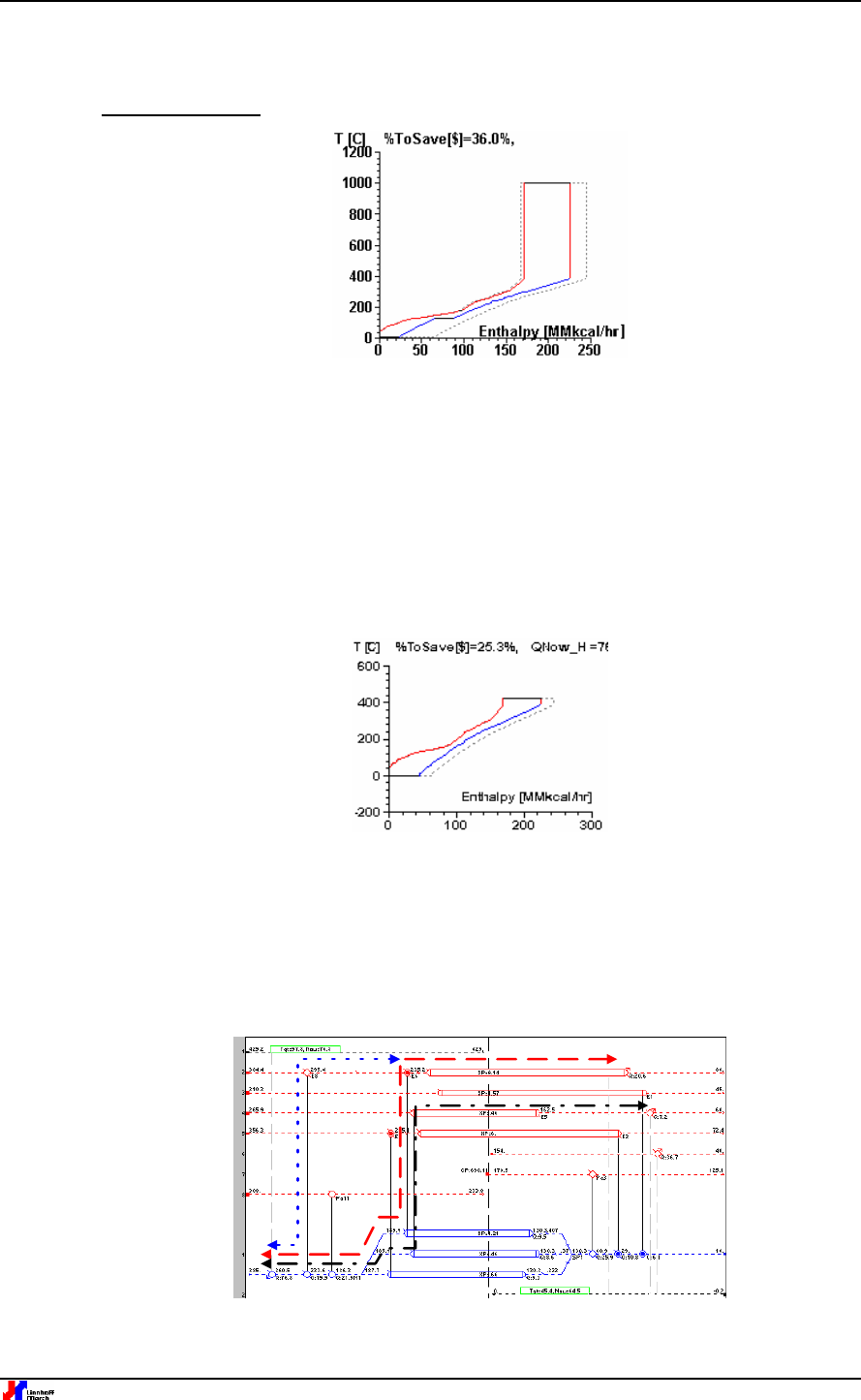
Introduction to Pinch Technology

Retrofit Example

Figure 44: Example requiring Path Analysis for retrofit design

An example with parallel composites and little requirement for intermediate utilities is shown

in Figure 44. Although the savings potential is large, the contribution from intermediate utilities

is not significant. This therefore means that to achieve the full savings, heat that is presently

rejected to cooling water must be recovered into cold process streams that presently rely on

furnace duty. This heat shift involves a wide temperature span and the modifications required

will be nearly equivalent to a complete re-design of the existing network. In order to avoid

such major changes, it is often preferred to identify opportunities where fewer modifications

can be made to achieve some of the potential savings.

Figure 45: Parallel composite curves with no intermediate utilities.

For the example shown in Figure 44, we can conduct the study with 1 hot utility and one cold

utility. The corresponding set of balanced composite curves is shown in Figure 45. This

greatly simplifies the design by removing 3 intermediate utilities whilst only reducing the

potential savings by a small amount. To achieve the energy savings, the hot and cold utility

requirements must be reduced by 19 MMkcal/h.

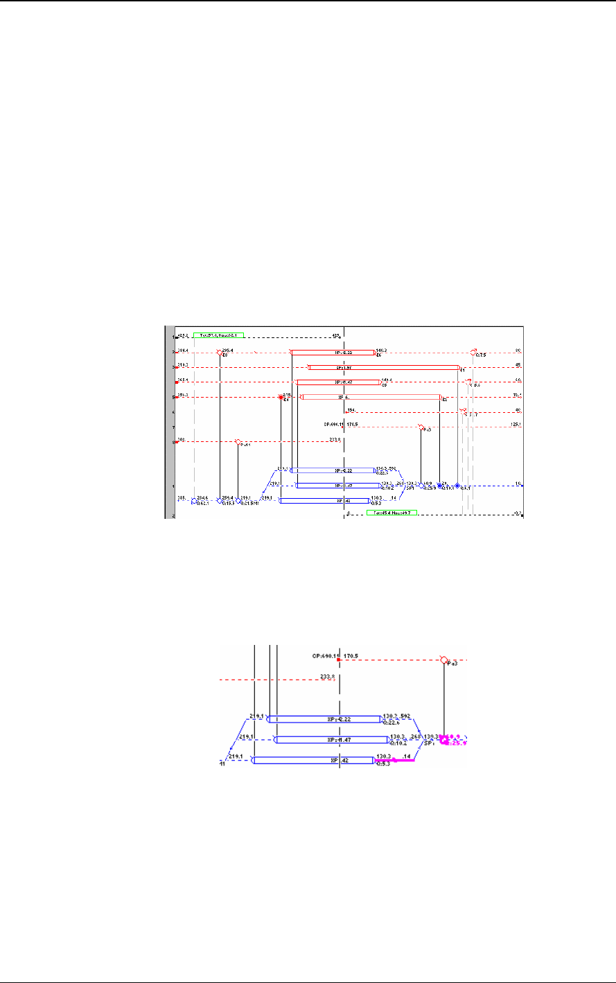
Introduction to Pinch Technology

Figure 46: Paths in the existing network

There are 3 heat load paths in the existing network and they link two of the three coolers to

the heater, Figure 46. The maximum additional heat recovery that can be achieved by

modifying the exchangers on these paths is the sum of the two cooler duties, which is, 28

MMkcal/h. If exchanger driving forces allow, the duty of the coolers can be reduced by

increasing the duty of exchangers E5, E6 and E8.

In order to know how much each of the exchangers should be increased by, it is necessary to

define a minimum approach temperature (EMAT) for the exchangers. This sets a limit on the

heat duty of the exchangers on the path. With a minimum approach of 10°C set for this

example, the duty of the three exchangers can be increased as shown below.

• E6, from 9.46 MMkcal/h to 22.58 MMkcal/h. This removes the opportunity to increase E8.

• E5 from 8.60 MMkcal/hr to 10.22 MMkcal/h

Figure 47: Modifying two paths saves 14.74MMkcal/h.

By increasing the duties of these two exchangers forming a path, a saving of 14.74 MMkcal/h

has been achieved, see Figure 47. The full potential is 19.1 MMkcal/h. To save the remaining

4.36 MMkcal/h, it is necessary to make some modifications to the network to increase the

driving force on these two exchangers.

Figure 48: Drag and drop of exchanger to a new position improves driving force on path

exchangers

A simple way to modify the network structure is by using the drag and drop tool in

PinchExpress to move an exchanger from one position to another. For instance, the minimum

approach temperature of 10°C occurs at the cold-end of exchangers E5 and E6. This can be

dealt with by moving one of the three exchangers below the split junction to above the split

junction. For instance, if exchanger pa3 can be moved to another position, the inlet

temperature to the exchangers at the split junction will be 60.9°C, instead of 130.3°. This

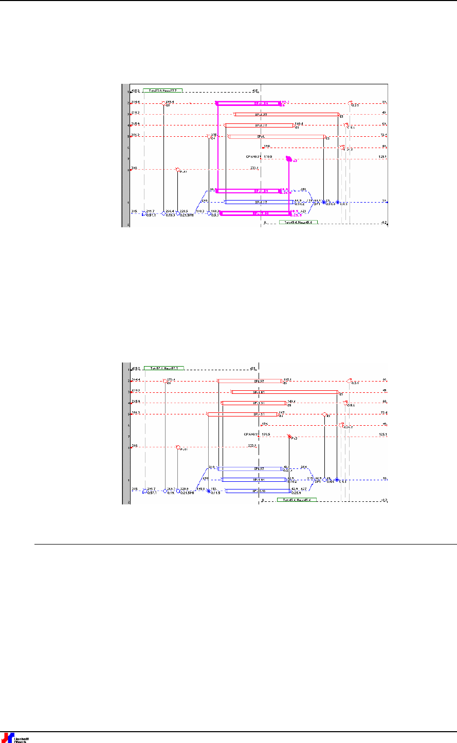
Introduction to Pinch Technology

means that the approach temperature for exchangers E5 and E6, at the cold end, becomes

79.4°C instead of 10°C. The improvement in driving force can then be used to increase the

duty of these exchangers on the paths, and further increase the energy savings.

Figure 49: With driving forces improved, the two paths can now be used to achieve the full

savings potential

In Figure 49, exchanger pa3 has been moved downstream of the splitter, just before E4. This

sufficiently opened up the driving force for E6 duty to be increased to 26.94 MMkcal/h. The

network shown in Figure 49 now meets the target hot and cold utility requirements. However,

it has an uneven distribution of temperature differences, which is likely to lead to a high

overall area requirement. This DT distribution can be improved by shifting heat around loops.

The final retrofit network, after re-distributing the driving forces is shown in Figure 50.

Figure 50: Final retrofit network.

10 Data Extraction Principles

This section covers in more depth the topic introduced in the earlier section "From Flowsheet

to Pinch Data" (section 3). PinchExpress carries out automatic Data Extraction. The

SuperTarget Process module also has this feature, plus additional facilities to allow users to

tailor the choices made in the data extraction procedure.

The required data involves process stream heating and cooling information, utility system

information, cost information and certain background information regarding the process and

the site.

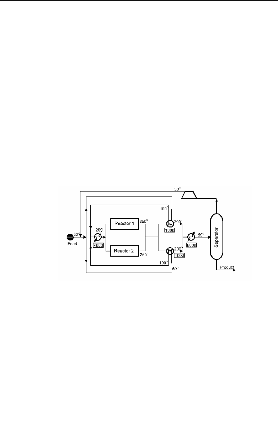
Introduction to Pinch Technology

The thermal data, which involves the stream heating and cooling information and utilities

information, is the most critical data required for pinch analysis.

There are several possibilities

for extracting the thermal data from a given heat and material balance. This must be done

carefully, as poor data extraction can easily lead to missed opportunities for improved

process design.

In extreme cases, poor data extraction can falsely present the existing

process flow-sheet as optimal in terms of energy efficiency.

If the data extraction accepts all

the features of the existing flow-sheet then there will be no scope for improvement. If it does

not accept any features of the existing flow-sheet then pinch analysis may over-estimate the

potential benefits. Appropriate data extraction accepts only the critical sections of the plant

which can not be changed. Data extraction skill develops with increased experience in the

application of pinch technology. However, over the years, simple heuristic rules have been

developed for data extraction.

In this section these rules are covered in more detail. Since the

quality of the final results in many cases depends on the quality of data extraction it is

important to understand the significance of these rules.

10.1 Do not carry over features of the existing solution

This rule is illustrated with the example below. Figure 51 shows an example process flow-

sheet.

Figure 51: Example Process Flowsheet

Figure 52 shows a literal data extraction from the flow-sheet on an exchanger by exchanger

basis resulting in the network design on the right. This network design is identical to the one

in the original flow-sheet.

The engineer performing the study would naturally conclude that the

original design is optimal and that the application of pinch technology has resulted in no

benefit.

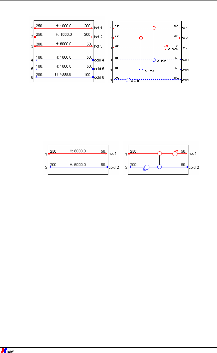
Introduction to Pinch Technology

Figure 52: Original Data Extraction and Design

Figure 53 shows an appropriate method of data extraction from the flow-sheet.

All the three

cold streams previously extracted can be equated to just one cold stream as shown, and

likewise only one hot stream needs to be extracted.

The resulting design is much simpler from

capital cost view-point and shows significant additional potential for improved energy recovery

(the network can achieve much lower DT

min

). The “proper” data extraction does not close off

any potential energy saving opportunities.

Figure 53: Improved Data Extraction and Design

The message is simply that the engineer should be careful in separating the relevant stream

data from the solution features of the previous design.

This does require a certain skill and

experience along with some knowledge of the process itself.

However the principles

explained in the following sections [3] should make it possible for an experienced process

engineer without much experience in Pinch Technology to extract the data without significant

errors.

10.2 Do not mix streams at different temperatures

One common problem in data extraction occurs when the process flow-sheet involves the

mixing of process streams at different temperatures.

When the streams are at different

temperatures, the mixing junction then acts as a direct contact heat exchanger.

An existing

exchanger is clearly part of the existing feature and should not be extracted as it is with the

stream data. Figure 54 below illustrates the problems with such a data extraction. Figure

54(a) shows a part of an existing flow-sheet where two process streams at different

temperatures are mixed together.

The mixing junction could involve cross-pinch heat transfer,

as shown in Figure 54(b), and therefore increase the overall process energy requirement.

avoid this, it is advised that if mixing must take place due to process reasons, the streams

involved in mixing should be extracted as being mixed at the same temperature as illustrated

in Figure 54(c).

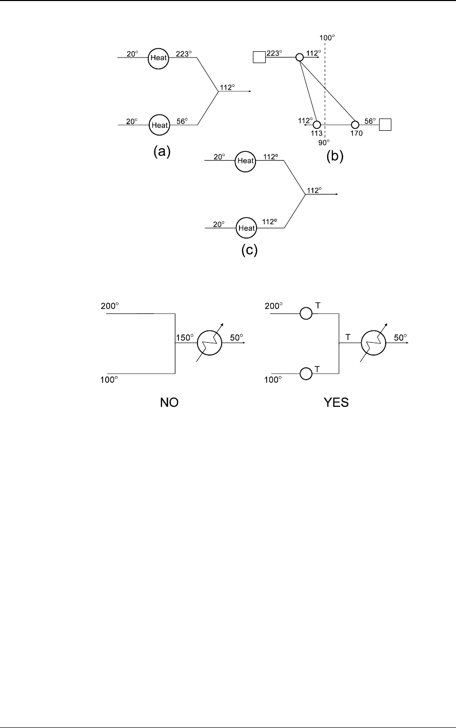
Introduction to Pinch Technology

Figure 54: Mixing at different temperatures may involve in-efficient cross-pinch heat transfer

thus increasing the energy requirement.

Figure 55: Isothermal mixing avoids cross-pinch heat transfer so do not mix at different

temperatures.

Figure 55 summarises the data extraction rule regarding non-isothermal mixing in flowsheets.

The correct data extraction must consider isothermal mixing.

The temperature for isothermal

mixing (T) can be chosen according to convenience.

This rule has significant benefit but can imply significant changes to the process flowsheet.

For example, the existing heat exchangers will no longer match the stream duty. For this

reason it is not applied automatically in PinchExpress. Instead, the rule must be applied

manually by changing the simulation or editing the data after transferral into PinchExpress. In

SuperTarget Process, however, the user is indeed given the option of applying the rule

automatically.

10.3 Extract at effective temperatures

For data extraction, the effective stream temperatures are more important than the actual

stream temperatures. For example, for a hot stream it is important to know what temperature

it is available at to exchange heat against cold streams, rather than its actual temperature.

Similarly, for cold streams it is the temperature at which heat must be supplied to them that is

important.

Consider the example in Figure 56.

A reactor product stream is released at 1000°C

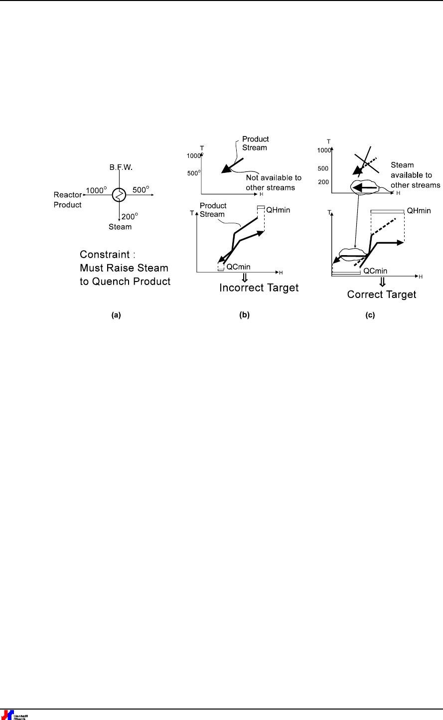
Introduction to Pinch Technology

and is to be cooled to 500°C.

The important feature of this product cooling is that it must be

quenched, during which steam is raised (e.g. ethylene process reactor product quenching).

As a result of this restriction, the temperature at which the heat in the product stream is

available to other streams is not 1000°C to 500ºC but the temperature at which steam is

raised.

It would be incorrect to extract the stream temperatures as from 1000°C to 500°C.

The

energy target would be over-optimistic.

Extracting at the effective temperature (condensing

steam temperature) gives the correct target.

Figure 56: Every stream must be extracted at the temperature at which it is available to other

process streams.

10.4 Extract streams on the safe side

The enthalpy change of some streams is significantly non-linear.

This is particularly true for

condensing/vaporising streams.

In such situations, adopting just one value of CP might lead

to inaccurate results.

It is more accurate to represent the stream in as many “segments” as is

required to closely mimic the heating and cooling curve of the stream.

However, the position

of the extracted stream with respect to the actual stream curve is also important.

In Figure

57(a), the extracted stream (straight line) is colder than the actual stream at the high

temperature end.

If there is a hot stream hot enough for the extracted stream but not hot

enough for the actual stream, an infeasible match will result. Figure 57(b) features safe side

extraction because the actual cold stream is colder than each of the three extracted

segments.

To linearise on the safe side (Figure 57(c)) therefore means that:

• The actual hot stream must be hotter than the extracted hot stream

• The actual cold stream must be colder than the extracted cold stream

Introduction to Pinch Technology

Figure 57: Stream linearisation,

a) and b) could be infeasible, c) is safe side linearisation.

This is not an issue when data is transferred to PinchExpress from a simulation because

heating curves are reduced automatically. However, this issue should be kept in mind when

entering data manually, in which case it is up to the user to ensure that heating profiles are

accurately represented.

10.5 Do not extract true utility streams

A true utility stream is a utility stream (i.e., steam, cooling water, refrigerant etc.) that can in

principle be replaced by any other stream (process or utility) for heat exchange purposes.

true utility stream should not be therefore extracted as a part of the process.

An example of a

true utility is cooling water used in an exchanger.

Since the cooling water can be replaced by

air cooling, refrigerant cooling or process stream heating, this should not be extracted.

However, when steam is required in a shift reactor to enhance the shift process, the steam is

not a true utility.

This is because the steam is not just used for heating but is necessary for the

reaction and cannot be replaced by another stream.

In such a situation, the steam must be

extracted as a cold stream, to be heated from boiler feed-water conditions to the appropriate

steam temperature and pressure for the reaction, and then vaporised.

Another example that

is not so straightforward is when direct steam is used for reboiling a column.

If this steam is

used just for heating purposes and can be replaced by a reboiler serviced by hot oil, steam or

some other hot utility, it would be treated as a true utility and should not be extracted.

However, if the reboiling must be via direct injection of steam, then the steam is not a utility

and should be extracted as part of the process.

10.6 Identify soft data

The temperature, pressure and enthalpy conditions of some streams within a process are

open to change within certain limits.

Such stream data are termed as “soft” data. An example

of “soft” data is the pump discharge pressure immediately upstream to a vaporiser.

The pump

discharge pressure can be varied within certain limits resulting in a corresponding flexibility in

the vaporisation temperature which is therefore soft data.

Another example of soft data is the

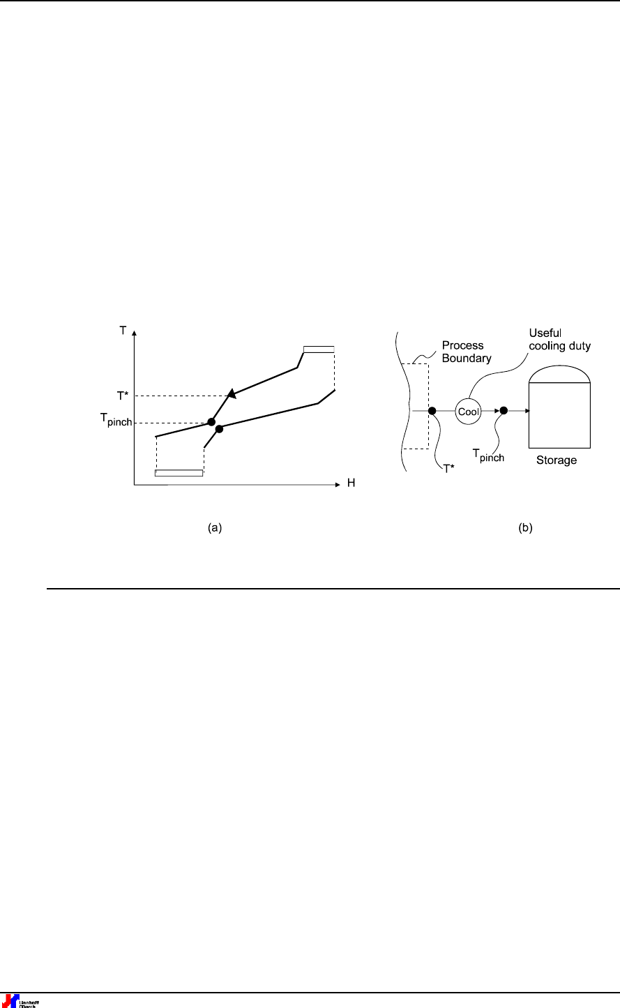
Introduction to Pinch Technology

target temperature of a product stream which is to go into storage. The temperature of the

stream going into a storage can be within a substantial temperature range.

Soft data should ideally be extracted such that the overall process energy requirement is

minimised.

For this, the (+)/(-) principle (section 7) for process modifications is applied.

With

the pump discharge pressure being a soft data, the feed vaporiser (a cold stream), should be

extracted at the coldest possible temperature.

In general, it is useful to view the preliminary set of composite curves before deciding how

best to extract the “soft data” as shown in Figure 58.

Figure 58(b) shows a product stream

leaving the process boundary at temperature T* for product storage.

Figure 58(a) shows the

composite curves for the overall process.

T* being greater than the pinch temperature (T

pinch

useful heat can still be extracted from the stream up to T

pinch

This will further reduce the hot

utility target based on the (+)/(-) principle.

The appropriate data extraction, therefore, in this

case is up to the pinch temperature.

Figure 58: Stream data extraction for “soft data”.

11 Total Site Improvement

Up to this point, heat and power targeting for a single process has been considered. Typically

refinery and petrochemical processes operate as parts of large sites or factories. These sites

have several processes serviced by a centralised utility system involved in steam and power

generation.

Introduction to Pinch Technology

Figure 59: Schematic of a site, showing production processes which are operated separately

from each other but are linked indirectly through the utility system.

Figure 59 shows a schematic of a typical process industry site involving several processes.

The production processes, some with their own utilities, are served by a common central

utility system. The utility system consumes fuel (e.g. gas and lignite), generates power and

supplies the necessary steam through several steam mains. There is both consumption and

recovery of process steam via the steam mains. Process furnaces also consume fuel. The

site imports or exports power to balance the on-site power generation. The process steam

heating and cooling demands and co-generation potential dictate the site-wide fuel demand

via the utility system.

Usually the individual production processes and the central services are controlled by

different departments. A number of different business units may occupy different subsections

of the site and operate independently. The site infrastructure therefore usually suffers from an

inadequate overview. To rectify it requires a simultaneous approach to consider individual

process issues alongside sitewide utility planning in the single context of making products

from feedstocks with minimum use of capital and energy in all forms. Total site improvement

using pinch technology provides an aid to sitewide planning for reduction in energy and

associated emissions. The SuperTarget Site module allows Engineers to undertake the type of

total site projects described in this section.

11.1 Total site data extraction

The heating and cooling requirements of the individual processes are represented by their

respective grand composite curves (section 5). The grand composite curve lays open the

process-utility interface for a single process. The grand composite curves can be used in

identifying potential heat recovery via steam mains for a small number of processes. However, for

a site involving several production processes (say 40), the grand composite curve of each

process will suggest different steam levels. The identification of correct compromise in steam

levels and loads will therefore become quite complex for a realistic site.

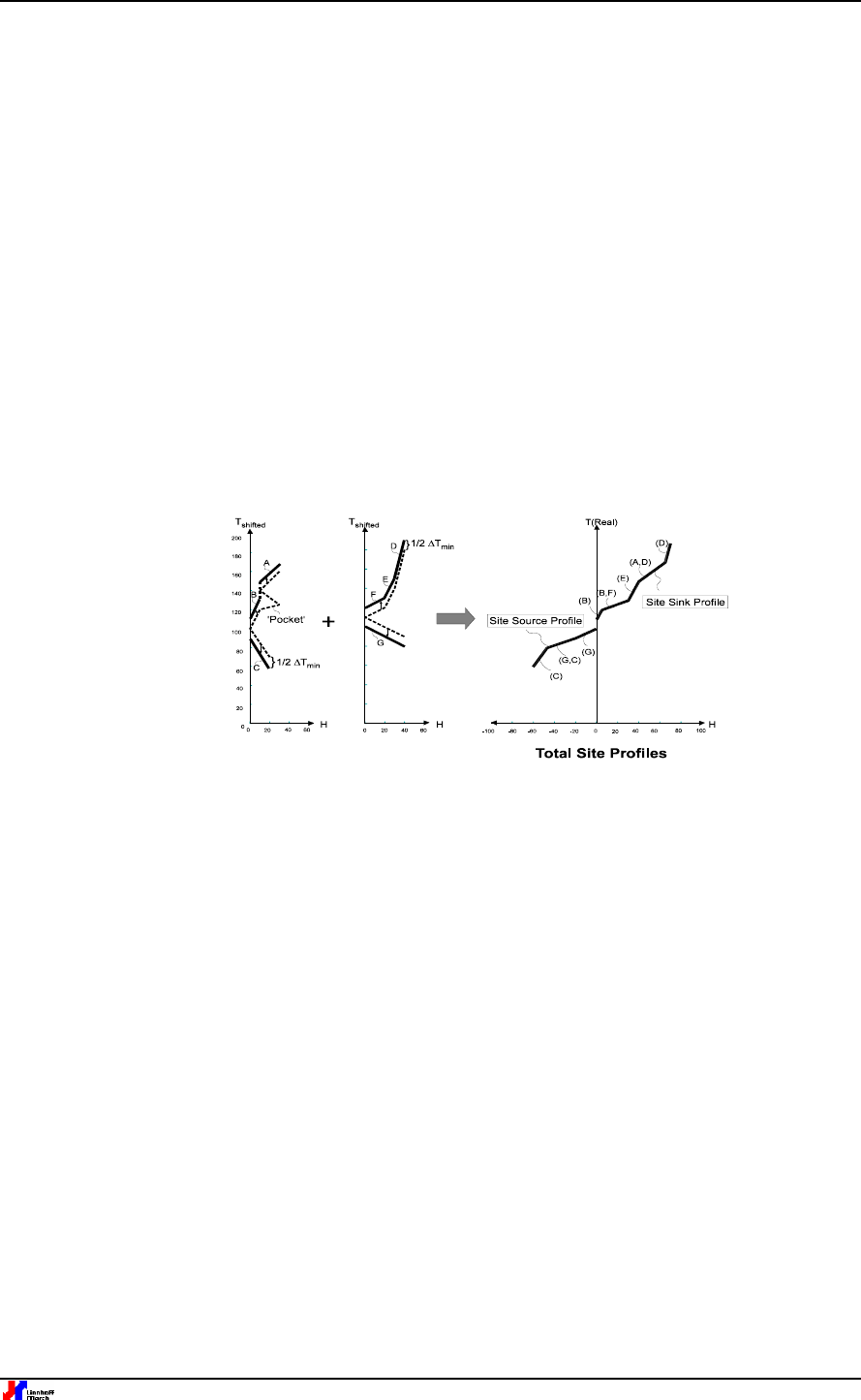
Introduction to Pinch Technology

11.1.1 Constructing Total Site Profiles

Pinch technology enables the designer to set utility targets for sites involving several processes

[10, 20]. This capability is based on thermal profiles for the entire site called the "total site

profiles". Total site profiles are constructed from the grand composite curves of the processes in

the site. Figure 60 illustrates the construction of the total site profiles using only two processes

(for demonstration purposes only). The construction starts with the grand composite curves of the

individual processes as shown in the figure. Prior to the construction of the total site profiles the

grand composite curves are then modified in two ways:

i) Parts of the grand composite curves that are satisfied by the central utility system are

isolated. The non monotonic parts, or the "pockets", in the individual grand composite curves

are sealed off through vertical lines as shown in Figure 60. Also parts of the curve directly

satisfied by a non-central utility (such as furnace heating within a process) are excluded from

the analysis. The remaining parts are the net heat source and sink elements to be satisfied by

the central utility system. The source elements as identified in the figure are C and G while

the sink elements are A, B, D, E and F as shown in Figure 60.

Figure 60: Construction of Total Site Profiles from process grand composite curves

ii) The source and sink elements of the resulting grand composite curves are shifted by 1/2

min

. Source element temperatures are reduced by 1/2 DT

min

while the sink element

temperatures are increased by 1/2 DT

min

as shown in Figure 60. This temperature shift

reverts the temperature scale back from shifted to real temperatures.

The construction of the total site profiles from the modified grand composite curves is also

shown in Figure 60. The construction simply involves the generation of "Composite Curves"

from the shifted source and sink elements. The composite of the source elements is called

the "Site Source Profile" while that of the sink elements is called the "Site Sink Profile". For

illustration purposes, the individual sink elements (A, B, D, E and F) and source elements (C

and G) have been highlighted throughout Figure 60. The temperature shift as shown in Figure

60 ensures that the total site profiles are in real temperatures.

11.1.2 Adding steam users not accounted in process stream data

Site source sink profiles primarily originate from the process grand composite curves. There

are other steam requirements which are not represented in the grand composite curve. These

are:

• Steam for ejectors, reactors, etc.

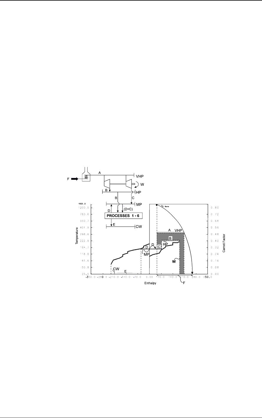
Introduction to Pinch Technology

• Tracing steam

• Unaccountable steam usage

These need to be considered in determining the correct utility system for the site. These

steam demands are considered as sink elements and are added to the site sink profile

without any temperature correction.

11.2 Total site analysis

11.2.1 Setting total site targets

The total site targets are developed via a combined use of Total Site Profiles and a Steam

System Simulator (e.g. Linnhoff March's Steam package) [10, 20]. Figure 61 illustrates site-

wide utilities targeting based on total site profiles and steam system simulation. The figure

shows the corresponding utilities schematic and total site profiles with the utilities placed

appropriately. Note that the vertical axis is now changed from temperature to Carnot factor (1-

/T). This allows direct visualisation of co-generation as shown by the shaded area in Figure

61.

Figure 61: Total site targeting for fuel, co-generation, emissions and cooling

The target for MP steam generation from all the processes is D. This partly satisfies the MP

demand. The remaining targeted MP demand (C) is provided by the turbine system. The

targeted HP steam demand for all the processes is (B). Thus the turbine system needs to

satisfy MP steam demand (C) and HP steam demand (B). Using steam system simulation

software the co-generation (W) and generating steam requirement at VHP level (A) are

calculated. The shaded area also indicates co-generation (W). From the VHP load the fuel

requirement (F) can be calculated using a standard boiler model in the steam system

simulator. This is indicated by a horizontal projection of the fuel profile on the enthalpy axis on

total site profiles. Knowing the fuel composition the fuel related emissions can be calculated.

The cooling demand for the total site as identified by the total site profiles is E. Thus starting

from individual process grand composite curves and using a steam system simulator targets

can be set for site fuel, co-generation, site emissions and cooling. The steam level placement

against total site profiles is in real temperatures the same as the total site profiles.

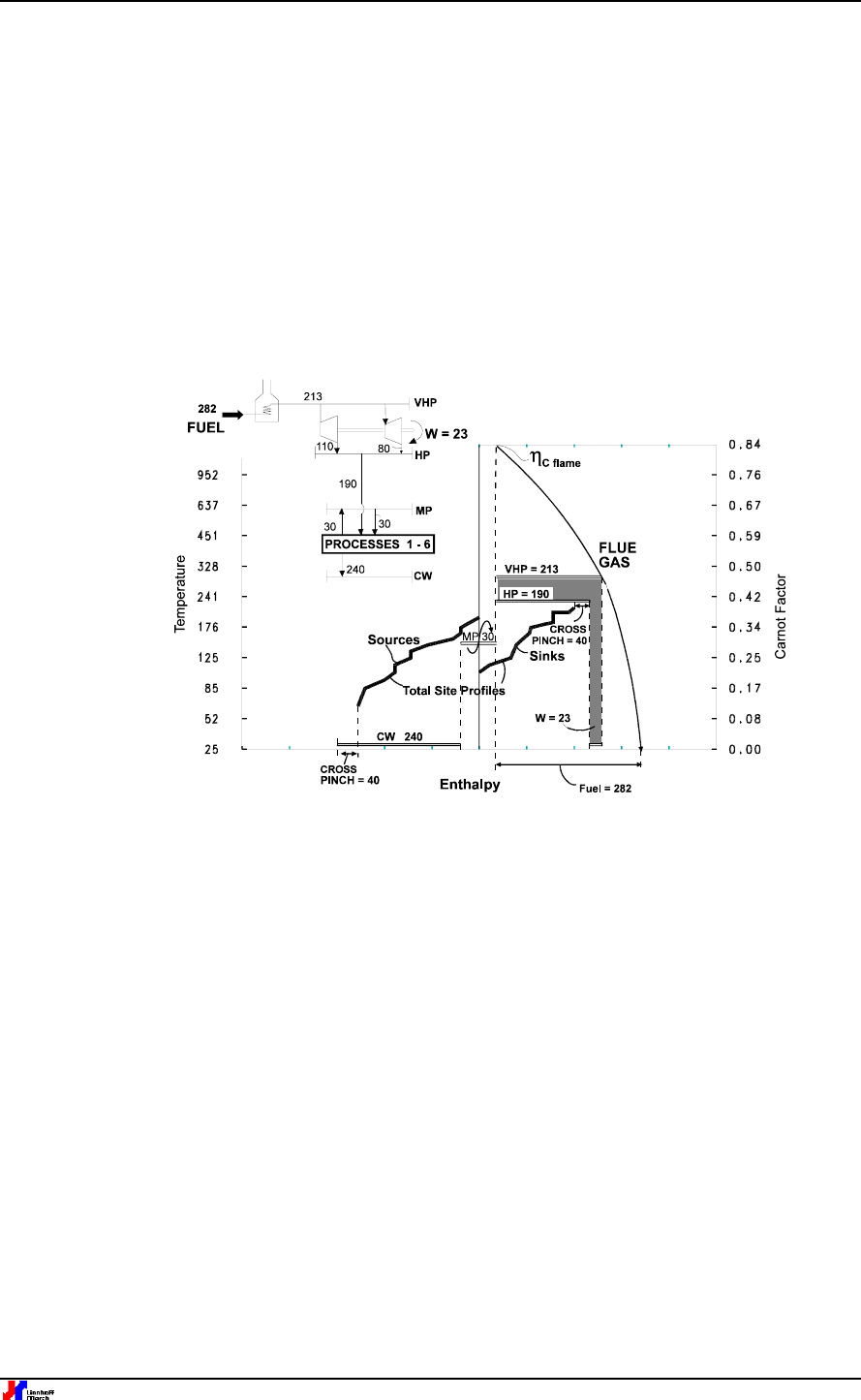
Introduction to Pinch Technology

The steam system simulation involves the simulation of the turbine system and the boiler

house. The model can be used to evaluate the co-generation and fuel consumption. In

addition the model can be used to check the constraints of the existing equipment along with

changes in steam demand, steam level, fuel type, power demand, utility costs, boiler feed

water heating etc.

11.2.2 Case study - Total site analysis

The use of total site profiles is illustrated with the following example, which relates to a site

expansion project [10, 20]. The example shows how the procedure can identify options that

result in significant capital cost savings and lower operating costs than conventional

solutions.

Figure 62: Existing site

Figure 62 above shows the example site with six processes as operating prior to the

expansion project. The existing utility system and the total site profiles are shown. The high

pressure (HP) steam mains receives steam from the central turbine system(190 MW). The

medium pressure (MP) mains is not connected to the turbine system. At the MP level, steam

generation from the processes and consumption by the processes are in balance (30 MW

each). The total site profile construction reveals an overall cross pinch heat transfer (in all

processes and the utility system) of 40 MW. The site co-generation is 23 MW and site fuel

consumption is 282 MW.

A site expansion is planned that involves the introduction of a new process into the existing

site. Figure 63 shows the proposed expansion plan with total site profiles and a utility sketch.

Both the source and the sink profiles are enlarged as a result of the expansion.

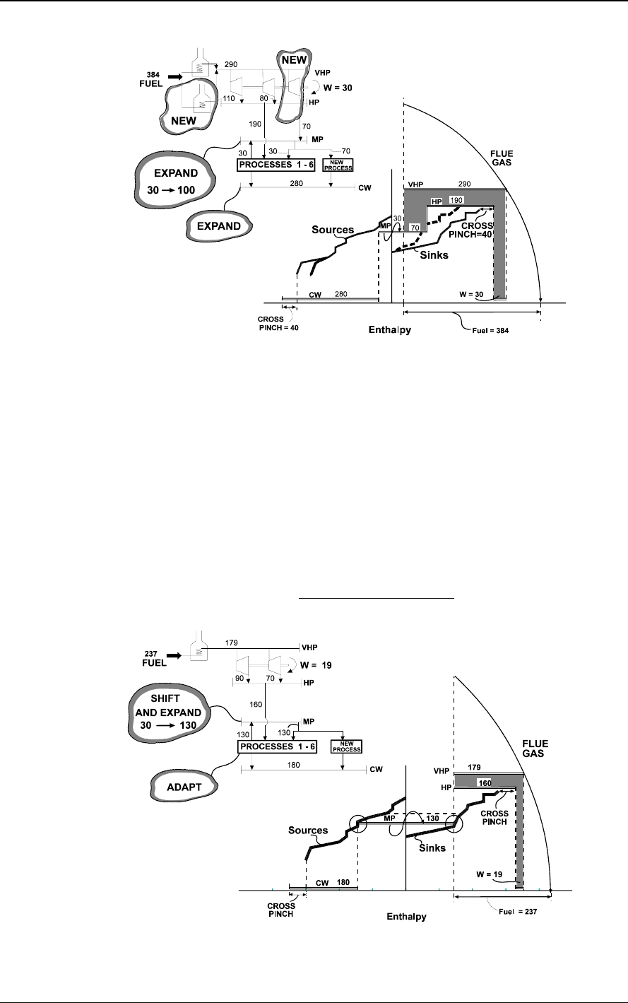
Introduction to Pinch Technology

Figure 63: Proposed expansion of the site involving addition of a new process

The initial study subjected the new process to a careful individual optimisation resulting in a

minimum energy requirement of 70 MW of MP steam. That steam is to be supplied via a new

turbine which links into the existing VHP and MP mains. In order to generate the additional

VHP steam (from 213 to 290 MW), a new boiler is planned. Also an expansion of the

cooling water system is necessary (from 240 to 280 MW).

However, the total site profiles reveal additional information. Since the profiles have changed

significantly as a result of the expansion, MP steam is no longer appropriate: it does not

exploit the driving forces available between the steam levels and the site sink profile. Pinch

analysis indicates that the MP steam pressure needs to be reduced. This is implemented in

Figure 64. The reduction in the MP steam pressure has been selected such that MP steam

generation is in balance with its use and its load is maximised

. Only a small pressure shift

was found necessary. As a consequence, the VHP steam demand is reduced significantly.

Figure 64: Alternative option based on Total Site Profiles

Introduction to Pinch Technology

Comparing the proposed expansion plan (Figure 63) with the alternative plan (Figure 64), it is

seen that there is reduction in energy and capital cost as well as a corresponding reduction in

emissions (see the table below). The alternative plan does not require investment in a new

turbine or a new boiler. It also does not require any expansion in the cooling capacity. The

alternative plan shows a reduction of 19% in the utilities operating cost and a global reduction

of 15% in emissions.

Proposed Design Alternative Design

Total utilities operating cost 100% 81%

(global) 100% 85%

Capital cost implications Expand MP steam Shift MP steam and expand

New turbine Adapt process to suit

New boiler

Expand cooling

Site power demand = 50 MW; cost data: fuel = $98/(kW.yr), power = $400/(kW.yr), cooling water =

$5/(kW.yr).

Table 5: Example case study: Comparison of operating and capital costs

Reference [10] provides further options involving process and utilities modifications for the

example case study.

By using the total site analysis, the most promising options for utilities and/or process can be

screened at the targeting stage. Since steam is simply an intermediate mechanism for heat

transfer, its cost is no longer a factor. All designs are directly evaluated in terms of fuel and

power at the site boundary.

References [1, 28, 30] provide information regarding applications of total site to real projects.

11.3 Selection of options: Total Site Road Map

Once the site has been translated to total site profiles, modelled with a steam system

simulation and different scenarios for site development have been explored, it is possible to

establish a relationship between investment and benefit of all the projects in the site. Such a

representation is called the “road map” for site development. Each route in a road-map

consists of a series of mutually compatible projects. Each project package is explored for its

technical and economic feasibility. The designer or planner can use the information from the

road-map to plan a “route” or a strategy for long term site development. Figure 65 shows an

example of a road map.

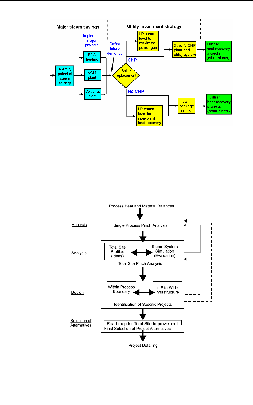
Introduction to Pinch Technology

Figure 65: Total Site Road Map

This approach provides a high level of confidence that the planning scenario offers the most

effective use of the capital. The total site road map can thus combine the information of

process wise improvements and sitewide improvements in one coherent plan.

11.3.1 Summary: Total Site Improvement

Figure 66 summarises the key steps in total site improvement based on pinch technology.

The key steps are listed as follows:

Figure 66: Key steps in total site improvement

a) Single Process Pinch Analysis: Starting from process heat and material balances of

individual processes, pinch analysis establishes key options for process modifications, energy

recovery (savings in non-central utilities) and targets for multiple utilities. The grand

Introduction to Pinch Technology

composite curves are ready for total site analysis. Initial trade-off is set between process fuel

and steam levels.

b) Total Site Pinch Analysis: Total site profiles are constructed from the individual process

grand composite curves and the site infrastructure (e.g. steam system) is simulated. These

tools are used together to set targets for infrastructure improvements and process wise

improvements. Re-visit step (a) and re-set infrastructure assumptions such as steam mains

pressures if they are changed in step (b).

c) Identification of Specific Projects: The targets obtained during individual process analysis

are translated into specific network design changes. Simultaneously, the infrastructure

improvement options are developed in more detail at an equipment level.

d) Final Selection of Project Alternatives (From Total Site Road Map): The specific projects

identified in step (c) are put together in a coherent plan for a total site involving alternative

routes of compatible projects. This is followed by final selection of process-wise and

infrastructure options for implementation. This stage is followed by project detailing.

Introduction to Pinch Technology

12 References

1. Linnhoff B, “Use Pinch Analysis to Knock Down Capital Costs and Emissions”, Chemical

Engineering Progress, August 1994.

2. Linnhoff B, D.W. Townsend, D. Boland, G.F. Hewitt, B.E.A. Thomas, A.R.Guy, and R.H.

Marsland, “User Guide on Process Integration for the Efficient Use of Energy”, IChemE,

Rugby, U.K. (1982).

3. Pinch Analysis Foundation Training Course, available from Linnhoff March Ltd, UK.

4. “SuperTarget” pinch analysis software suite, available from Linnhoff March Ltd, UK.

5. Townsend, D. W., and B. Linnhoff, “Heat and Power Networks in Process Design, Part I:

Criteria for Placement of Heat Engines and Heat Pumps in Process Networks”, AIChE J.,

29(5), pp. 742-748 (May 1983). “Part II: Design Procedure for Equipment Selection and

Process Matching”, AIChE J., 29(5), pp. 748-771 (May 1983).

6. Linnhoff, B, H Dunford, and R. Smith, “Heat Integration of Distillation Columns into

Overall Processes”, Chem. Eng. Sc., 38(8), pp. 1175-1188 (1983).

7. Smith, R., and P.S. Jones, “The Optimal Design of Integrated Evaporation Systems”,

Heat Recov. Sys. & CHP, 10 (4), pp. 341-368 (1990).

8. Linnhoff B, and S. Ahmad, “Cost Optimum Heat Exchanger Networks, Part 1: Minimum

Energy and Capital using Simple Models for Capital Cost“, Comp. & Chem. Eng. 14 (7),

pp. 729-750 (1990). Ahmad S., B. Linnhoff, and R. Smith, “Part 2: Targets and Design for

Detailed Capital Cost Models, “Comp. & Chem. Eng., 14 (7), pp. 751-767 (1990).

9. Tjoe, T. N., and B. Linnhoff, “Using Pinch Technology for Process Retrofit”, Chem. Eng.,

pp. 47-60 (Apr. 28, 1986).

10. Dhole, V. R., and B. Linnhoff, “Total Site Targets for Fuel, Co-generation, emissions, and

Cooling”, Comp. & Chem. Eng., 17 suppl. pp. s101-s109 (1993).

11. Linnhoff, B., and V.R.Dhole, “Shaftwork Targets for Low Temperature Process Design”,

Chem. Eng. Sci., 47 (8), pp. 2,081-2,091 (1992).

12. Dhole, V. R., and B. Linnhoff , “Overall Design of Subambient Plants”, Comp. and Chem.

Eng., 18, suppl. pp. s105-s111 (1994).

13. Linnhoff, B., and E. Kotjabasakis, “Process Optimisation: Downstream Paths for Operable

Process Design,” Chem. Eng. Progress, 82 (5), pp. 23-28 (May 1986).

14. Obeng, E. D. A., and G. J. Ashton, “On Pinch Technology Based Procedures for the

Design of Batch Processes”, Chem. Eng. Res. & Des., 66, pp. 225-259 (1988).

15. Dhole, V. R., and B. Linnhoff, “Distillation Column Targets”, Comp. & Chem. Eng., 17

(5/6), pp. 549-560 (1993).

16. Linnhoff B., and D. R. Vredeveld, “Pinch Technology Has Come Of Age”, Chem. Eng.

Progress, 80 (7), pp. 33-40 (July 1984).

Introduction to Pinch Technology

17. Linnhoff, B., and G. T. Polley, “Stepping Beyond the Pinch”, The Chem. Eng., pp/ 25-32

(Feb. 1988).

18. Smith, R., and B. Linnhoff, “The Design of Separators in the Context of Overall

Processes”, Chem. Eng. Res. & Des., 66, pp. 195-228 (May 1988).

19. Kotjabasakis, E., and b. Linnhoff, “Better System Design Reduces Heat Exchanger

Fouling Costs”, Oil & Gas J., pp. 49-56 (Sept. 1987).

20. Linnhoff, B., and V. R. Dhole, “Targeting for CO

Emissions for Total Sites”, Chem. Ing.

Tech., 16, pp. 256-259 (1993).

21. Rossiter, A. P., H. D. Spriggs, and H. Klee, Jr., “Apply Process Integration to Waste

Minimisation“, Chem. Eng. Progress, 89 (1), pp. 30-36 (Jan. 1993).

22. Smith, R., and E. A. Petela, “Waste Minimisation in the Process Industries”, “1: The

Problem”, The Chem. Eng., pp. 24-25 (Oct. 1991); “2: Reactors“, The Chem. Eng., pp.

17-23 (Dec. 1991); “3: Separation and Recycle Systems“, The Chem. Eng., pp. 24-28

(Feb. 1992); “4: Process Operations“, The Chem. Eng., pp. 21-23 (Apr. 1992); “5: Utility

Waste”, The Chem. Eng., pp. 32-35 (July 1992).

23. Morgan, S., “Use Process Integration to Improve Process Designs and the Design

Process“, Chem. Eng. Progress, 88 (9), pp. 62-68 (Sept. 1992).

24. Brown, K. J., “Process Integration Initiative” (review of the process integration initiatives

funded under the Energy Efficiency R&D Programme), Energy Technology Support Unit,

Harwell Laboratory, Didcot, U.K. (July 1989).

25. Natori, Y., “Managing the Implementation of Pinch Technology in a Large Company”,

presented at the IEA Workshop on Process Integration, Gothenburg, Sweden (Jan.

1992).

26. Trivedi, K. K., K. H. Pang, H. R. Klavers, D. L. O’Young, and B. Linnhoff, “Integrated

Ethylene Process Design using Pinch Technology”, presented at AIChE Meeting, Atlanta

(Apr. 1994).

27. Snoek, J., and T. N. Tjoe, “Process Integration Experience in a Large Company”,

presented at the IEA Workshop on Process Integration, Gothenburg, Sweden (Jan.

1992).

28. Rudman, A., et al., “Experience from Total site Integration”, Linnhoff March International,

Northwich, U.K. (1994).

29. Obata, K., and H. Shibuya, “The Challenge of Minimum Energy Plant Design”, presented

at Ascope 93. Bangkok (Nov. 1993).

30. Yoda, H., H. Shibuya, “An approach to Minimum Energy Plant Design Incorporating Pinch

Technology and State-of-the-Art Equipment”, presented at the 1995 NPRA Annual

Meeting, San Francisco, California (Mar. 1995).