FUNDAMENTALS OF DIFFERENTIAL EQUATIONS
SEVENTH EDITION
AND
FUNDAMENTALS OF DIFFERENTIAL EQUATIONS
AND
BOUNDARY VALUE PROBLEMS
FIFTH EDITION
R. Kent Nagle
University of South Florida
Edward B. Saff
Vanderbilt University
A. David Snider
University of South Florida
INSTRUCTOR’S
SOLUTIONS MANUAL
388445_Nagle_ttl.qxd 1/9/08 11:53 AM Page 1
Reproduced by Pearson Addison-Wesley from electronic files supplied by the author.
Copyright © 2008 Pearson Education, Inc.
Publishing as Pearson Addison-Wesley, 75 Arlington Street, Boston, MA 02116.
All rights reserved. No part of this publication may be reproduced, stored in a retrieval system, or trans-
mitted, in any form or by any means, electronic, mechanical, photocopying, recording, or otherwise, with-
out the prior written permission of the publisher.
ISBN-13: 978-0-321-38844-5
ISBN-10: 0-321-38844-5
This work is protected by United States copyright laws and is provided solely
for the use of instructors in teaching their courses and assessing student
learning. Dissemination or sale of any part of this work (including on the
World Wide Web) will destroy the integrity of the work and is not permit-
ted. The work and materials from it should never be made available to
students except by instructors using the accompanying text in their
classes
. All recipients of this work are expected to abide by these
restrictions and to honor the intended pedagogical purposes and the needs of
other instructors who rely on these materials.
388445_Nagle_ttl.qxd 1/9/08 11:53 AM Page 2
Contents
Notes to the Instructor 1
Software Supplements . . . . . . . . . . . . . . . . . . . . . . . . . . . . . . . . 1
Computer Labs . . . . . . . . . . . . . . . . . . . . . . . . . . . . . . . . . . . 1
Group Projects . . . . . . . . . . . . . . . . . . . . . . . . . . . . . . . . . . . . 2
Technical Writing Exercises . . . . . . . . . . . . . . . . . . . . . . . . . . . . . 2
Student Presentations . . . . . . . . . . . . . . . . . . . . . . . . . . . . . . . . 2
Homework Assignments . . . . . . . . . . . . . . . . . . . . . . . . . . . . . . . 3
Syllabus Suggestions . . . . . . . . . . . . . . . . . . . . . . . . . . . . . . . . . 3
Numerical, Graphical, and Qualitative Methods . . . . . . . . . . . . . . . . . . 4
Engineering/Physics Applications . . . . . . . . . . . . . . . . . . . . . . . . . 5
Biology/Ecology Applications . . . . . . . . . . . . . . . . . . . . . . . . . . . . 7
Supplemental Group Projects 9
Detailed Solutions & Answers to Even-Numbered Problems 17
CHAPTER 1 Introduction 17
Exercises 1.1 Detailed Solutions . . . . . . . . . . . . . . . . . . . . . . . . . 17
Exercises 1.2 Detailed Solutions . . . . . . . . . . . . . . . . . . . . . . . . . 18
Exercises 1.3 Detailed Solutions . . . . . . . . . . . . . . . . . . . . . . . . . 22
Exercises 1.4 Detailed Solutions . . . . . . . . . . . . . . . . . . . . . . . . . 25
Tables . . . . . . . . . . . . . . . . . . . . . . . . . . . . . . . . . . . . . . . . 28
Figures . . . . . . . . . . . . . . . . . . . . . . . . . . . . . . . . . . . . . . . 29
CHAPTER 2 First Order Differential Equations 35
Exercises 2.2 Detailed Solutions . . . . . . . . . . . . . . . . . . . . . . . . . 35
Exercises 2.3 Detailed Solutions . . . . . . . . . . . . . . . . . . . . . . . . . 41
Exercises 2.4 Detailed Solutions . . . . . . . . . . . . . . . . . . . . . . . . . 48
Exercises 2.5 Detailed Solutions . . . . . . . . . . . . . . . . . . . . . . . . . 56
Exercises 2.6 Detailed Solutions . . . . . . . . . . . . . . . . . . . . . . . . . 61
Review Problems Answers . . . . . . . . . . . . . . . . . . . . . . . . . . . . 70
Tables . . . . . . . . . . . . . . . . . . . . . . . . . . . . . . . . . . . . . . . . 71
Figures . . . . . . . . . . . . . . . . . . . . . . . . . . . . . . . . . . . . . . . 71
iii
CHAPTER 3 Mathematical Models and Numerical Methods
Involving First Order Equations 73
Exercises 3.2 Detailed Solutions . . . . . . . . . . . . . . . . . . . . . . . . . 73
Exercises 3.3 Detailed Solutions . . . . . . . . . . . . . . . . . . . . . . . . . 81
Exercises 3.4 Detailed Solutions . . . . . . . . . . . . . . . . . . . . . . . . . 87
Exercises 3.5 Answers . . . . . . . . . . . . . . . . . . . . . . . . . . . . . . . 96
Exercises 3.6 Answers . . . . . . . . . . . . . . . . . . . . . . . . . . . . . . . 97
Exercises 3.7 Answers . . . . . . . . . . . . . . . . . . . . . . . . . . . . . . . 97
Tables . . . . . . . . . . . . . . . . . . . . . . . . . . . . . . . . . . . . . . . . 98
Figures . . . . . . . . . . . . . . . . . . . . . . . . . . . . . . . . . . . . . . . 100
CHAPTER 4 Linear Second Order Equations 101
Exercises 4.1 Detailed Solutions . . . . . . . . . . . . . . . . . . . . . . . . . 101
Exercises 4.2 Detailed Solutions . . . . . . . . . . . . . . . . . . . . . . . . . 103
Exercises 4.3 Detailed Solutions . . . . . . . . . . . . . . . . . . . . . . . . . 111
Exercises 4.4 Detailed Solutions . . . . . . . . . . . . . . . . . . . . . . . . . 119
Exercises 4.5 Detailed Solutions . . . . . . . . . . . . . . . . . . . . . . . . . 125
Exercises 4.6 Detailed Solutions . . . . . . . . . . . . . . . . . . . . . . . . . 137
Exercises 4.7 Detailed Solutions . . . . . . . . . . . . . . . . . . . . . . . . . 144
Exercises 4.8 Detailed Solutions . . . . . . . . . . . . . . . . . . . . . . . . . 157
Exercises 4.9 Detailed Solutions . . . . . . . . . . . . . . . . . . . . . . . . . 160
Exercises 4.10 Detailed Solutions . . . . . . . . . . . . . . . . . . . . . . . . . 167
Review Problems Answers . . . . . . . . . . . . . . . . . . . . . . . . . . . . 172
Figures . . . . . . . . . . . . . . . . . . . . . . . . . . . . . . . . . . . . . . . 173
CHAPTER 5 Introduction to Systems and Phase Plane Analysis 177
Exercises 5.2 Answers . . . . . . . . . . . . . . . . . . . . . . . . . . . . . . . 177
Exercises 5.3 Answers . . . . . . . . . . . . . . . . . . . . . . . . . . . . . . . 179
Exercises 5.4 Answers . . . . . . . . . . . . . . . . . . . . . . . . . . . . . . . 180
Exercises 5.5 Answers . . . . . . . . . . . . . . . . . . . . . . . . . . . . . . . 182
Exercises 5.6 Answers . . . . . . . . . . . . . . . . . . . . . . . . . . . . . . . 182
Exercises 5.7 Answers . . . . . . . . . . . . . . . . . . . . . . . . . . . . . . . 183
Exercises 5.8 Answers . . . . . . . . . . . . . . . . . . . . . . . . . . . . . . . 183
Review Problems Answers . . . . . . . . . . . . . . . . . . . . . . . . . . . . 184
Tables . . . . . . . . . . . . . . . . . . . . . . . . . . . . . . . . . . . . . . . . 185
Figures . . . . . . . . . . . . . . . . . . . . . . . . . . . . . . . . . . . . . . . 187
CHAPTER 6 Theory of Higher-Order Linear Differential Equations 193
Exercises 6.1 Answers . . . . . . . . . . . . . . . . . . . . . . . . . . . . . . . 193
Exercises 6.2 Answers . . . . . . . . . . . . . . . . . . . . . . . . . . . . . . . 194
Exercises 6.3 Answers . . . . . . . . . . . . . . . . . . . . . . . . . . . . . . . 194
Exercises 6.4 Answers . . . . . . . . . . . . . . . . . . . . . . . . . . . . . . . 195
iv
Review Problems Answers . . . . . . . . . . . . . . . . . . . . . . . . . . . . 196
CHAPTER 7 Laplace Transforms 197
Exercises 7.2 Detailed Solutions . . . . . . . . . . . . . . . . . . . . . . . . . 197
Exercises 7.3 Detailed Solutions . . . . . . . . . . . . . . . . . . . . . . . . . 201
Exercises 7.4 Detailed Solutions . . . . . . . . . . . . . . . . . . . . . . . . . 206
Exercises 7.5 Detailed Solutions . . . . . . . . . . . . . . . . . . . . . . . . . 215
Exercises 7.6 Detailed Solutions . . . . . . . . . . . . . . . . . . . . . . . . . 224
Exercises 7.7 Detailed Solutions . . . . . . . . . . . . . . . . . . . . . . . . . 239
Exercises 7.8 Detailed Solutions . . . . . . . . . . . . . . . . . . . . . . . . . 247
Exercises 7.9 Detailed Solutions . . . . . . . . . . . . . . . . . . . . . . . . . 252
Review Problems Answers . . . . . . . . . . . . . . . . . . . . . . . . . . . . 262
Figures . . . . . . . . . . . . . . . . . . . . . . . . . . . . . . . . . . . . . . . 263
CHAPTER 8 Series Solutions of Differ ential E quations 267
Exercises 8.1 Answers . . . . . . . . . . . . . . . . . . . . . . . . . . . . . . . 267
Exercises 8.2 Answers . . . . . . . . . . . . . . . . . . . . . . . . . . . . . . . 268
Exercises 8.3 Answers . . . . . . . . . . . . . . . . . . . . . . . . . . . . . . . 269
Exercises 8.4 Answers . . . . . . . . . . . . . . . . . . . . . . . . . . . . . . . 270
Exercises 8.5 Answers . . . . . . . . . . . . . . . . . . . . . . . . . . . . . . . 271
Exercises 8.6 Answers . . . . . . . . . . . . . . . . . . . . . . . . . . . . . . . 271
Exercises 8.7 Answers . . . . . . . . . . . . . . . . . . . . . . . . . . . . . . . 273
Exercises 8.8 Answers . . . . . . . . . . . . . . . . . . . . . . . . . . . . . . . 274
Review Problems Answers . . . . . . . . . . . . . . . . . . . . . . . . . . . . 275
Figures . . . . . . . . . . . . . . . . . . . . . . . . . . . . . . . . . . . . . . . 276
CHAPTER 9 Matrix Methods for Linear Systems 277
Exercises 9.1 Answers . . . . . . . . . . . . . . . . . . . . . . . . . . . . . . . 277
Exercises 9.2 Answers . . . . . . . . . . . . . . . . . . . . . . . . . . . . . . . 277
Exercises 9.3 Answers . . . . . . . . . . . . . . . . . . . . . . . . . . . . . . . 278
Exercises 9.4 Answers . . . . . . . . . . . . . . . . . . . . . . . . . . . . . . . 280
Exercises 9.5 Answers . . . . . . . . . . . . . . . . . . . . . . . . . . . . . . . 282
Exercises 9.6 Answers . . . . . . . . . . . . . . . . . . . . . . . . . . . . . . . 285
Exercises 9.7 Answers . . . . . . . . . . . . . . . . . . . . . . . . . . . . . . . 286
Exercises 9.8 Answers . . . . . . . . . . . . . . . . . . . . . . . . . . . . . . . 287
Review Problems Answers . . . . . . . . . . . . . . . . . . . . . . . . . . . . 289
Figures . . . . . . . . . . . . . . . . . . . . . . . . . . . . . . . . . . . . . . . 290
CHAPTER 10 Partial Differential Equations 291
Exercises 10.2 Answers . . . . . . . . . . . . . . . . . . . . . . . . . . . . . . 291
Exercises 10.3 Answers . . . . . . . . . . . . . . . . . . . . . . . . . . . . . . 291
Exercises 10.4 Answers . . . . . . . . . . . . . . . . . . . . . . . . . . . . . . 292
v
Exercises 10.5 Answers . . . . . . . . . . . . . . . . . . . . . . . . . . . . . . 293
Exercises 10.6 Answers . . . . . . . . . . . . . . . . . . . . . . . . . . . . . . 294
Exercises 10.7 Answers . . . . . . . . . . . . . . . . . . . . . . . . . . . . . . 295
CHAPTER 11 Eigenvalue Problems and Sturm-Liouville Equations 297
Exercises 11.2 Answers . . . . . . . . . . . . . . . . . . . . . . . . . . . . . . 297
Exercises 11.3 Answers . . . . . . . . . . . . . . . . . . . . . . . . . . . . . . 298
Exercises 11.4 Answers . . . . . . . . . . . . . . . . . . . . . . . . . . . . . . 298
Exercises 11.5 Answers . . . . . . . . . . . . . . . . . . . . . . . . . . . . . . 299
Exercises 11.6 Answers . . . . . . . . . . . . . . . . . . . . . . . . . . . . . . 300
Exercises 11.7 Answers . . . . . . . . . . . . . . . . . . . . . . . . . . . . . . 302
Exercises 11.8 Answers . . . . . . . . . . . . . . . . . . . . . . . . . . . . . . 303
Review Problems Answers . . . . . . . . . . . . . . . . . . . . . . . . . . . . 303
CHAPTER 12 Stability of Autonomous Systems 305
Exercises 12.2 Answers . . . . . . . . . . . . . . . . . . . . . . . . . . . . . . 305
Exercises 12.3 Answers . . . . . . . . . . . . . . . . . . . . . . . . . . . . . . 305
Exercises 12.4 Answers . . . . . . . . . . . . . . . . . . . . . . . . . . . . . . 306
Exercises 12.5 Answers . . . . . . . . . . . . . . . . . . . . . . . . . . . . . . 306
Exercises 12.6 Answers . . . . . . . . . . . . . . . . . . . . . . . . . . . . . . 307
Exercises 12.7 Answers . . . . . . . . . . . . . . . . . . . . . . . . . . . . . . 307
Review Problems Answers . . . . . . . . . . . . . . . . . . . . . . . . . . . . 308
Figures . . . . . . . . . . . . . . . . . . . . . . . . . . . . . . . . . . . . . . . 309
CHAPTER 13 Existence and Uniqueness Theory 317
Exercises 13.1 Answers . . . . . . . . . . . . . . . . . . . . . . . . . . . . . . 317
Exercises 13.2 Answers . . . . . . . . . . . . . . . . . . . . . . . . . . . . . . 317
Exercises 13.3 Answers . . . . . . . . . . . . . . . . . . . . . . . . . . . . . . 318
Exercises 13.4 Answers . . . . . . . . . . . . . . . . . . . . . . . . . . . . . . 318
Review Problems Answers . . . . . . . . . . . . . . . . . . . . . . . . . . . . 318
vi
Notes to the Instructor
One goal in our writing has been to create flexible texts that afford the instructor a variety
of topics and make available to the student an abundance of practice problems and projects.
We recommend that the instructor read the discus sion given in the preface in order to gain
an overview of the prerequisites, topics of emphasis, and general philosophy of the text.
Software Supplements
Interactive Differential Equations CD-ROM: By Beverly West (Cornell University),
Steven Strogatz (Cornell University), Jean Marie McDill (California Polytechnic State Uni-
versity – San Luis Obispo), John Cantwell (St. Louis University), and Hubert Hohn (Mas-
sachusetts College of Arts) is a popular software directly tied to the text that focuses on helping
students visualize concepts. Applications are drawn from engineering, physics, chemistry, and
biology. Runs on Windows or Macintosh and is included free with every book.
Instructor’s MAPLE/MATHLAB/MATHEMATICA manual: By Thomas W. Po-
laski (Winthrop University), Bruno Welfert (Arizona State University), and Maurino Bautista
(Rochester Institute of Technology). A collection of worksheets and projects to aid instruc-
tors in integrating computer algebra systems into their courses. Available via Addison-Wesley
Instructor’s Resource Center.
MATLAB Manual ISBN 13: 978-0-321-53015-8; ISBN 10: 0-321-53015-2
MAPLE Manual ISBN 13: 978-0-321-38842-1; ISBN 10: 0-321-38842-9
MATHEMATICA Manual ISBN 13: 978-0-321-52178-1; ISBN 10: 0-321-52178-1
Computer Labs
A computer lab in connection with a differential equations course can add a whole new di-
mension to the teaching and learning of differential equations. As more and more colleges
and universities set up computer labs with software such as MAPLE, MATLAB, DERIVE,
MATHEMATICA, PHASEPLANE, and MACMATH, there will b e more opportunities to in-
clude a lab as part of the differential equations course. In our teaching and in our texts, we
have tried to provide a variety of exercises, problems, and projects that encourage the student
to use the computer to explore. Even one or two hours at a computer generating phase plane
diagrams can provide the students with a feeling of how they will use technology together
1
with the theory to investigate real world problems. Furthermore, our experience is that they
thoroughly enjoy these activities. Of course, the software, provided free with the texts, is
especially convenient for such labs.
Group Projects
Although the projects that appear at the end of the chapters in the text can be worked
out by the conscientious student working alone, making them group projects adds a soc ial
element that encourages discussion and interactions that simulate a professional work place
atmosphere. Group sizes of 3 or 4 seem to be optimal. Moreover, requiring that each individual
student separately write up the group’s solution as a formal technical report for grading by
the instructor also contributes to the professional flavor.
Typically, our students each work on 3 or 4 projects per semester. If class time permits, oral
presentations by the groups can be scheduled and help to improve the communication skills
of the students.
The role of the instructor is, of course, to help the students solve these elaborate problems on
their own and to recommend additional reference material when appropriate.
Some additional Group Projects are presented in this guide (see page 9).
Technical Writing Exercises
The technical writing exercises at the end of most chapters invite students to make documented
responses to questions dealing with the concepts in the chapter. This not only gives students
an opportunity to improve their writing skills, but it helps them organize their thoughts and
better understand the new concepts. Moreover, many questions deal with critical thinking
skills that will be useful in their careers as engineers, scientists, or mathematicians.
Since most students have little experience with technical writing, it may b e necessary to return
ungraded the first few technical writing assignments with comments and have the students redo
the the exercise. This has worked well in our classes and is much appreciated by the students.
Handing out a “model” technical writing response is also helpful for the students.
Student Presentations
It is not uncommon for an instructor to have students go to the board and present a solution
2
to a problem. Differential equations is so rich in theory and applications that it is an excellent
course to allow (require) a student to give a presentation on a special application (e.g., almost
any topic from Chapter 3 and 5), on a new technique not covered in class (e.g., material from
Section 2.6, Projects A, B, or C in Chapter 4), or on additional theory (e.g., material from
Chapter 6 which generalizes the results in Chapter 4). In addition to improving students’
communication skills, these “special” topics are long remembered by the students. Here, too,
working in groups of 3 or 4 and sharing the presentation responsibilities can add substantially
to the interest and quality of the presentation. Students should also be encouraged to enliven
their communication by building physical models, preparing part of their lectures on video
cassette, etc.
Homework Assignments
We would like to share with you an obvious, non-original, but effective method to encourage
students to do homework problems.
An essential feature is that it requires little extra work on the part of the instructor or grader.
We assign homework problems (about 10 of them) after each lecture. At the end of the week
(Fridays), students are asked to turn in their homework (typically, 3 sets) for that week. We
then choose at random one problem from each assignment (typically, a total of 3) that will
be graded. (The point is that the student does not know in advance which problems will be
chosen.) Full credit is given for any of the chosen problems for which there is evidence that the
student has made an honest attempt at solving. The homework problem sets are returned to
the students at the next meeting (Mondays) with grades like 0/3, 1/3, 2/3, or 3/3 indicating
the proportion of problems for which the student received credit. The homework grades are
tallied at the end of the semester and count as one test grade. Certainly, there are variations
on this theme. The point is that students are motivated to do their homework with little
additional cost (= time) to the instructor.
Syllabus Suggestions
To serve as a guide in constructing a syllabus for a one-s emester or two-semester course, the
prefaces to the texts list sample outlines that emphasize methods, applications, theory, partial
differential equations, phase plane analysis, computation, or combinations of these. As a
further guide in making a choice of subject matter, we provide below a listing of text material
dealing with some common areas of emphasis.
3
Numerical, Graphical, and Qualitative Methods
The sections and projects dealing with numerical, graphical, and qualitative techniques of
solving differential equations include:
Section 1.3: Direction Fields
Section 1.4: The Approximation Method of Euler
Project A for Chapter 1: Taylor Series
Project B for Chapter 1: Picard’s Method
Project D for Chapter 1: The Phase Line
Section 3.6: Improved Euler’s Method, which includes step-by-step outlines of the im-
proved Euler’s method subroutine and improved Euler’s method with tolerance. These
outlines are easy for the student to translate into a computer program (cf. pages 135
and 136).
Section 3.7: Higher-Order Numerical Methods : Taylor and Runge-Kutta, which includes
outlines for the Fourth Order Runge-Kutta subroutine and algorithm with tolerance (see
pages 144 and 145).
Project H for Chapter 3: Stability of Numerical Methods
Project I for Chapter 3: Period Doubling an Chaos
Section 4.8: Qualitative Considerations for Variable Coefficient and Nonlinear Equa-
tions, which discusses the energy integral lemma, as well as the Airy, Bessel, Duffing,
and van der Pol equations.
Section 5.3: Solving Systems and Higher-Order Equations Numerically, which describes
the vectorized forms of Euler’s method and the Fourth Order Runge-Kutta method, and
discusses an application to population dynamics.
Section 5.4: Introduction to the Phase Plane, which introduces the study of trajectories
of autonomous systems, critical points, and stability.
4
Section 5.8: Dynamical Systems, Poincar`e Maps, and Chaos, which discusses the use of
numerical methods to approximate the Poincar`e map and how to interpret the results.
Project A for Chapter 5: Designing a Landing System for Interplanetary Travel
Project B for Chapter 5: Things That Bob
Project D for Chapter 5: Strange Behavior of Competing Species – Part I
Project D for Chapter 9: Strange Behavior of Competing Species – Part II
Project D for Chapter 10: Numerical Method for ∆u = f on a Rectangle
Project D for Chapter 11: Shooting Method
Project E for Chapter 11: Finite-Difference Method for Boundary Value Problems
Project C for Chapter 12: Computing Phase Plane Diagrams
Project D for Chapter 12: Ecosystem of Planet GLIA-2
Appendix A: Newton’s Method
Appendix B: Simpson’s Rule
Appendix D: Method of Least Squares
Appendix E: Runge-Kutta Procedure for Equations
The instructor who wishes to emphasize numerical methods should also note that the text
contains an extensive chapter of series solutions of differential e quations (Chapter 8).
Engineering/Physics Applications
Since Laplace transforms is a subject vital to engineering, we have included a detailed chapter
on this topic – see Chapter 7. Stability is also an important subject for engineers, so we
have included an introduction to the subject in Chapter 5.4 along with an entire chapter
addressing this topic – see Chapter 12. Further material dealing with engineering/physic
applications include:
Project C for Chapter 1: Magnetic “Dipole”
5
Project B for Chapter 2: Torricelli’s Law of Fluid Flow
Section 3.1: Mathematical Modeling
Section 3.2: Compartmental Analysis, which contains a discussion of mixing problems
and of population models.
Section 3.3: Heating and Cooling Buildings, which discusses temperature variations in
the presence of air conditioning or furnace heating.
Section 3.4: Newtonian Mechanics
Section 3.5: Electrical Circuits
Project C for Chapter 3: Curve of Pursuit
Project D for Chapter 3: Aircraft Guidance in a Crosswind
Project E for Chapter 3: Feedback and the Op Amp
Project F for Chapter 3: Band-Bang Controls
Section 4.1: Introduction: Mass-Spring Oscillator
Section 4.8: Qualitative Considerations for Variable-Coefficient and Nonlinear Equations
Section 4.9: A Closer Look at Free Mechanical Vibrations
Section 4.10: A Closer Look at Forced Mechanical Vibrations
Project B for Chapter 4: Apollo Reentry
Project C for Chapter 4: Simple Pendulum
Chapter 5: Introduction to Systems and Phase Plane Analysis, which includes sections
on coupled mass-spring systems, electrical circuits, and phase plane analysis.
Project A for Chapter 5: Designing a Landing System for Interplanetary Travel
Project B for Chapter 5: Things that Bob
Project C for Chapter 5: Hamiltonian Systems
6
Project D for Chapter 5: Transverse Vibrations of a Beam
Chapter 7: Laplace Transforms, which in addition to basic material includes discussions
of transfer functions, the Dirac delta function, and frequency response mode ling.
Projects for Chapter 8, dealing with Schr¨odinger’s equation, bucking of a tower, and
again springs.
Project B for Chapter 9: Matrix Laplace Transform Method
Project C for Chapter 9: Undamped Second-Order Systems
Chapter 10: Partial Differential Equations, which includes sections on Fourier series, the
heat equation, wave equation, and Laplace’s equation.
Project A for Chapter 10: Steady-State Temperature Distribution in a Circular Cylinder
Project B for Chapter 10: A Laplace Transform Solution of the Wave Equation
Project A for Chapter 11: Hermite Polynomials and the Harmonic O scillator
Section 12.4: Energy Methods, which addresses both conservative and nonconservative
autonomous mechanical systems.
Project A for Chapter 12: Solitons and Korteweg-de Vries Equation
Project B for Chapter 12: Burger’s Equation
Students of engineering and physics would also find Chapter 8 on series solutions particularly
useful, especially Section 8.8 on special functions.
Biology/Ecology Applications
Project D f or Chapter 1: The Phase Plane, which discusses the logistic population model
and bifurcation diagrams for p opulation control.
Project A for Chapter 2: Differential Equations in Clinical Medicine
Section 3.1: Mathematical Modeling
7
Section 3.2: Compartmental Analysis, which contains a discussion of mixing problems
and population models.
Project A for Chapter 3: Dynamics for HIV Infection
Project B for Chapter 3: Aquaculture, which deals with a model of raising and harvesting
catfish.
Section 5.1: Interconnected Fluid Tanks, which introduces systems of equations.
Section 5.3: Solving Systems and Higher-Order Equations Numerically, which contains
an application to population dynamics.
Section 5.5: Applications to Biomathematics: Epidemic and Tumor Growth Models
Project D for Chapter 5: Strange Behavior of Competing Species – Part I
Project E for Chapter 5: Cleaning Up the Great Lakes
Project D for Chapter 9: Strange Behavior of Competing Species – Part II
Problem 19 in Exercises 10.5 , which involves chemical diffusion through a thin layer.
Project D for Chapter 12: Ecosystem on Planet GLIA-2
The basic content of the remainder of this instructor’s manual consists of supplemental group
projects, answers to the even-numbered problems, and detailed solutions to the even-numbered
problems in Chapters 1, 2, 4, and 7 as well as Sections 3.2, 3.3, and 3.4. The answers are,
for the most part, not available any place else since the text only provides answers to odd-
numbered problems, and the Student’s Solutions Manual contains only a handful of worked
solutions to even-numbered problems.
We would appreciate any comments you may have concerning the answers in this manual.
These comments can be sent to the authors’ email addresses below. We also would encourage
sharing with us (= the authors and users of the texts) any of your favorite group projects.
E. B. Saff A. D. Snider
Edward.B.Saff@Vanderbilt.edu [email protected]
8

Group Projects for Chapter 3
Delay Differential Equations
In our discussion of mixing problems in Section 3.2, we encountered the initial value
problem
x
0
(t) = 6 −
3
500
x (t − t
0
) , (0.1)
x(t) = 0 for x ∈ [−t
0
, 0] ,
where t
0
is a positive constant. The equation in (0.1) is an example of a delay differ-
ential equation. These equations differ from the usual differential equations by the
presence of the shift (t − t
0
) in the argument of the unknown function x(t). In general,
these equations are more difficult to work with than are regular differential equations,
but quite a bit is known about them.
1
(a) Show that the simple linear delay differential equation
x
0
= ax(t − b), (0.2)
where a, b are constants, has a solution of the form x(t) = Ce
st
for any constant
C, provided s satisfies the transcendental equation s = ae
−bs
.
(b) A solution to (0.2) for t > 0 can also be found using the method of steps. Assume
that x(t) = f(t) for −b ≤ t ≤ 0. For 0 ≤ t ≤ b, equation (0.2) becomes
x
0
(t) = ax(t −b) = af(t −b),
and so
x(t) =
t
Z
0
af(ν − b)dν + x(0).
Now that we know x(t) on [0, b], we can repeat this procedure to obtain
x(t) =
t
Z
b
ax(ν − b)dν + x(b)
for b ≤ x ≤ 2b. This process can be continued indefinitely.
1
See, for example, Differential–Difference Equations, by R. Bellman and K. L. Cooke, Academic Press, New
York, 1963, or Ordinary and Delay Differential Equations, by R. D. Driver, Springer–Verlag, New York, 1977
9

Use the method of steps to show that the solution to the initial value problem
x
0
(t) = −x(t −1), x(t) = 1 on [−1, 0],
is given by
x(t) =
n
X
k=0
(−1)
k
[t − (k − 1)]
k
k!
, for n − 1 ≤ t ≤ n ,
where n is a nonnegative integer. (This problem can also be solved using the
Laplace transform method of Chapter 7.)
(c) Use the method of steps to compute the solution to the initial value problem given
in (0.1) on the interval 0 ≤ t ≤ 15 for t
0
= 3.
Extrapolation
When precise information about the form of the error in an approximation is known, a
technique called extrapolation can be used to improve the rate of convergence.
Suppose the approximation method converges with rate O (h
p
) as h → 0 (cf. Section 3.6).
From theoretical considerations, assume we know, more precisely, that
y(x; h) = φ(x) + h
p
a
p
(x) + O
h
p+1
, (0.3)
where y(x; h) is the approximation to φ(x) using step size h and a
p
(x) is some function
that is independent of h (typically, we do not know a formula for a
p
(x), only that it
exists). Our goal is to obtain approximations that converge at the faster rate O (h
p+1
).
We start by replacing h by h/2 in (0.3) to get
y
x;
h
2
= φ(x) +
h
p
2
p
a
p
(x) + O
h
p+1
.
If we multiply both sides by 2
p
and subtract equation (0.3), we find
2
p
y
x;
h
2
− y(x; h) = (2
p
− 1) φ(x) + O
h
p+1
.
Solving for φ(x) yields
φ(x) =
2
p
y (x; h/2) − y(x; h)
2
p
− 1
+ O
h
p+1
.
Hence,
y
∗
x;
h
2
:=
2
p
y (x; h/2) − y(x; h)
2
p
− 1
has a rate of convergence of O (h
p+1
).
10

(a) Assuming
y
∗
x;
h
2
= φ(x) + h
p+1
a
p+1
(x) + O
h
p+2
,
show that
y
∗∗
x;
h
4
:=
2
p+1
y
∗
(x; h/4) − y
∗
(x; h/2)
2
p+1
− 1
has a rate of convergence of O (h
p+2
).
(b) Assuming
y
∗∗
x;
h
4
= φ(x) + h
p+2
a
p+2
(x) + O
h
p+3
,
show that
y
∗∗∗
x;
h
8
:=
2
p+2
y
∗∗
(x; h/8) − y
∗∗
(x; h/4)
2
p+2
− 1
has a rate of convergence of O (h
p+3
).
(c) The results of using Euler’s method (with h = 1, 1/2, 1/4, 1/8) to approximate the
solution to the initial value problem
y
0
= y, y(0) = 1
at x = 1 are given in Table 1.2, page 27. For Euler’s method, the extrapolation
procedure applies with p = 1. Use the results in Table 1.2 to find an approximation
to e = y(1) by computing y
∗∗∗
(1; 1/8). [Hint: Compute y
∗
(1; 1/2), y
∗
(1; 1/4), and
y
∗
(1; 1/8); then compute y
∗∗
(1; 1/4) and y
∗∗
(1; 1/8).]
(d) Table 1.2 also contains Euler’s approximation for y(1) when h = 1/16. Use this
additional information to compute the next step in the extrapolation procedure;
that is, compute y
∗∗∗∗
(1; 1/16).
Group Projects for Chapter 5
Effects of Hunting on Predator–Prey Systems
As discussed in Section 5.3 (page 277), cyclic variations in the population of predators
and their prey have been studied using the Volterra-Lotka predator–prey model
dx
dt
= Ax − Bxy , (0.4)
dy
dt
= −Cy + Dxy , (0.5)
11
where A, B, C, and D are positive constants, x(t) is the population of prey at time t, and
y(t) is the population of predators. It can be shown that such a system has a periodic
solution (see Project D). That is, there exists some constant T such that x(t) = x(t + T )
and y(t) = y(t + T ) for all t. The periodic or cyclic variation in the population has
been observed in various systems such as sharks–food fish, lynx–rabbits, and ladybird
beetles–cottony cushion scale. Because of this periodic behavior, it is useful to consider
the average population x and y defined by
x :=
1
T
t
Z
0
x(t)dt , y :=
1
T
t
Z
0
y(t)dt .
(a) Show that x = C/D and y = A/B. [Hint: Use equation (0.4) and the fact that
x(0) = x(T ) to show that
T
Z
0
[A − By(t)] dt =
T
Z
0
x
0
(t)
x(t)
d =
dt
0. ]
(b) To determine the effect of indiscriminate hunting on the population, assume hunting
reduces the rate of change in a population by a constant times the population. Then
the predator–prey system satisfies the new set of equations
dx
dt
= Ax − Bxy − εx = (A −ε)x −Bxy , (0.6)
dy
dt
= −Cy + Dxy − δy = −(C + δ)y + Dxy , (0.7)
where ε and δ are positive constants with ε < A. What effect does this have on the
average population of prey? On the average population of predators?
(c) Assume the hunting was done selectively, as in shooting only rabbits (or shooting
only lynx). Then we have ε > 0 and δ = 0 (or ε = 0 and δ > 0) in (0.6)–(0.7).
What effect does this have on the average populations of predator and prey?
(d) In a rural county, foxes prey mainly on rabbits but occasionally include a chicken
in their diet. The farmers decide to put a stop to the chicken killing by hunting
the foxes. What do you predict will happen? What will happen to the farmers’
gardens?
12

Limit Cycles
In the study of triode vacuum tubes, one encounters the van der Pol equation
2
y
00
− µ
1 − y
2
y
0
+ y = 0 ,
where the constant µ is regarded as a parameter. In Section 4.8 (page 224), we used the
mass-spring oscillator analogy to argue that the nonzero solutions to the van der Pol
equation with µ = 1 should approach a periodic limit cycle. The same argument applies
for any positive value of µ.
(a) Recast the van der Pol equation as a system in normal form and use software to
plot some typical trajectories for µ = 0.1, 1, and 10. Re-scale the plots if necess ary
until you can discern the limit cycle trajectory; find trajectories that spiral in, and
ones that spiral out, to the limit cycle.
(b) Now let µ = −0.1, −1, and −10. Try to predict the nature of the solutions using
the mass-spring analogy. Then use the software to check your predictions. Are
there limit cycles? Do the neighboring trajectories spiral into, or spiral out from,
the limit cycles?
(c) Repeat parts (a) and (b) for the Rayleigh equation
y
00
− µ
h
1 − (y
0
)
2
i
y
0
+ y = 0 .
Group Project for Chapter 13
David Stapleton, University of Central Oklahoma
Satellite Altitude Stability
In this problem, we determine the orientation at which a satellite in a circular orbit of
radius r can maintain a relatively constant facing with respect to a spherical primary
(e.g., a planet) of mass M. The torque of gravity on the asymmetric satellite maintains
the orientation.
2
Historical Footnote: Experimental research by E. V. Appleton and B. van der Pol in 1921 on the
oscillation of an electrical circuit containing a triode generator (vacuum tube) led to the nonlinear e quation
now called van der Pol’s equation. Methods of solution were developed by van der Pol in 1926–1927.
Mary L. Cartwright continued research into nonlinear oscillation theory and together with J. E. Little-
wood obtained existence results for forced oscillations in nonlinear systems in 1945.
13
Suppose (x, y, z) and (x, y, z) refer to coordinates in two systems that have a common
origin at the satellite’s center of mass. Fix the xyz-axes in the satellite as principal axes;
then let the z-axis point toward the primary and let the x-axis point in the direction of
the satellite’s velocity. The xyz-axes may be rotated to coincide with the xyz-axes by
a rotation φ ab out the x-axis (roll), followed by a rotation θ about the resulting y-axis
(pitch), and a rotation ψ about the final z-axis (yaw). Euler’s equations from physics
(with high terms omitted
3
to obtain approximate solutions valid near (φ, θ, ψ) = (0, 0, 0))
show that the equations for the rotational motion due to gravity acting on the satellite
are
I
x
φ
00
= −4ω
2
0
(I
z
− I
y
) φ − ω
0
(I
y
− I
z
− I
x
) ψ
0
I
y
θ
00
= −3ω
2
0
(I
x
− I
z
) θ
I
z
ψ
00
= −4ω
2
0
(I
y
− I
x
) ψ + ω
0
(I
y
− I
z
− I
x
) φ
0
,
where ω
0
=
p
(GM)/r
3
is the angular frequency of the orbit and the positive constants
I
x
, I
y
, I
z
are the moments of inertia of the satellite about the x, y, and z-axes.
(a) Find constants c
1
, . . . , c
5
such tha these equations can b e written as two systems
d
dt
φ
ψ
φ
0
θ
0
=
0 0 1 0
0 0 0 1
c
1
0 0 c
2
0 c
3
c
4
0
φ
ψ
φ
0
ψ
0
and
d
dt
"
θ
θ
0
#
=
"
0 1
c
5
0
#"
θ
θ
0
#
.
(b) Show that the origin is asymptotically stable for the first system in (a) if
(c
2
c
4
+ c
3
+ c
1
)
2
− 4c
1
c
3
> 0 ,
c
1
c
3
> 0 ,
c
2
c
4
+ c
3
+ c
1
> 0
and hence deduce that I
y
> I
x
> I
z
yields an asymptotically stable origin. Are
there other conditions on the moments of inertia by which the origin is stable?
3
The derivation of these equations is found in Attitude Stabilization and Control of Earth Satellites, by
O. H. Gerlach, Space Science Reviews, #4 (1965), 541–566
14
(c) Show that, for the asymptotically stable configuration in (b), the second system
in (a) becomes a harmonic oscillator problem, and find the f requency of oscillation
in terms of I
x
, I
y
, I
z
, and ω
0
. Phobos maintains I
y
> I
x
> I
z
in its orientation
with respect to Mars, and has angular frequency of orbit ω
0
= 0.82 rad/hr. If
(I
x
− I
z
) /I
y
= 0.23, show that the period of the libration for Phobos (the period
with which the side of Phobos facing Mars shakes back and forth) is about 9 hours.
15

CHAPTER 1: Introduction
EXERCISES 1.1: Background
2. This equation is an ODE because it contains no partial derivatives. Since the highest
order derivative is d
2
y/dx
2
, the equation is a second order equation. This same term
also shows us that the independent variable is x and the dependent variable is y. This
equation is linear.
4. This equation is a PDE of the second order because it contains second partial derivatives.
x and y are independent variables, and u is the dependent variable.
6. This equation is an ODE of the first order with the independent variable t and the
dependent variable x. It is nonlinear.
8. ODE of the second order with the independent variable x and the depende nt variable y,
nonlinear.
10. ODE of the fourth order with the inde pendent variable x and the dependent variable y,
linear.
12. ODE of the second order with the independent variable x and the depende nt variable y,
nonlinear.
14. The velocity at time t is the rate of change of the position function x(t), i.e., x
0
. Thus,
dx
dt
= kx
4
,
where k is the proportionality constant.
16. The equation is
dA
dt
= kA
2
,
where k is the proportionality constant.
17

Chapter 1
EXERCISES 1.2: Solutions and Initial Value Problems
2. (a) Writing the given equation in the form y
2
= 3 − x, we see that it defines two
functions of x on x ≤ 3, y = ±
√
3 − x. Differentiation yields
dy
dx
=
d
dx
±
√
3 − x
= ±
d
dx
(3 − x)
1/2
= ±
1
2
(3 − x)
−1/2
(−1) = −
1
±2
√
3 − x
= −
1
2y
.
(b) Solving for y yields
y
3
(x − x sin x) = 1 ⇒ y
3
=
1
x(1 − sin x)
⇒ y =
1
3
p
x(1 − sin x)
= [x(1 − sin x)]
−1/3
.
The domain of this function is x 6= 0 and
sin x 6= 1 ⇒ x 6=
π
2
+ 2kπ, k = 0, ±1, ±2, . . . .
For 0 < x < π/2, one has
dy
dx
=
d
dx
[x(1 − sin x)]
−1/3
= −
1
3
[x(1 − sin x)]
−1/3−1
d
dx
[x(1 − sin x)]
= −
1
3
[x(1 − sin x)]
−1
[x(1 − sin x)]
−1/3
[(1 − sin x) + x(−cos x)]
=
(x cos x + sin x − 1)y
3x(1 − sin x)
.
We also remark that the given relation is an implicit solution on any interval not
containing points x = 0, π/2 + 2kπ, k = 0, ±1, ±2, . . . .
4. Differentiating the function x = 2 cos t −3 sin t twice, we obtain
x
0
= −2 sin t − 3 cos t, x
00
= −2 cos t + 3 sin t.
Thus,
x
00
+ x = (−2 cos t + 3 sin t) + (2 cos t − 3 sin t) = 0
for any t on (−∞, ∞).
6. Substituting x = cos 2t and x
0
= −2 sin 2t into the given equation yields
(−2 sin 2t) + t cos 2t = sin 2t ⇔ t cos 2t = 3 sin 2t .
Clearly, this is not an identity and, therefore, the function x = cos 2t is not a solution.
18

Exercises 1.2
8. Using the chain rule, we have
y = 3 sin 2x + e
−x
,
y
0
= 3(cos 2x)(2x)
0
+ e
−x
(−x)
0
= 6 cos 2x − e
−x
,
y
00
= 6(−sin 2x)(2x)
0
− e
−x
(−x)
0
= −12 sin 2x + e
−x
.
Therefore,
y
00
+ 4y =
−12 sin 2x + e
−x
+ 4
3 sin 2x + e
−x
= 5e
−x
,
which is the right-hand side of the given equation. So, y = 3 sin 2x + e
−x
is a solution.
10. Taking derivatives of both sides of the given relation with respect to x yields
d
dx
(y − ln y) =
d
dx
x
2
+ 1
⇒
dy
dx
−
1
y
dy
dx
= 2x
⇒
dy
dx
1 −
1
y
= 2x ⇒
dy
dx
y − 1
y
= 2x ⇒
dy
dx
=
2xy
y − 1
.
Thus, the relation y−ln y = x
2
+1 is an implicit solution to the equation y
0
= 2xy/(y−1).
12. To find dy/dx, we use implicit differentiation.
d
dx
x
2
− sin(x + y)
=
d
dx
(1) = 0 ⇒ 2x − cos(x + y)
d
dx
(x + y) = 0
⇒ 2x − cos(x + y)
1 +
dy
dx
= 0 ⇒
dy
dx
=
2x
cos(x + y)
− 1 = 2x sec(x + y) − 1,
and so the given differential equation is satisfied.
14. Assuming that C
1
and C
2
are constants, we differentiate the function φ(x) twice to get
φ
0
(x) = C
1
cos x − C
2
sin x, φ
00
(x) = −C
1
sin x − C
2
cos x.
Therefore,
φ
00
+ φ = (−C
1
sin x − C
2
cos x) + (C
1
sin x + C
2
cos x) = 0.
Thus, φ(x) is a solution with any choice of constants C
1
and C
2
.
16. Differentiating both sides, we obtain
d
dx
x
2
+ Cy
2
=
d
dx
(1) = 0 ⇒ 2x + 2Cy
dy
dx
= 0 ⇒
dy
dx
= −
x
Cy
.
19

Chapter 1
Since, from the given relation, Cy
2
= 1 − x
2
, we have
−
x
Cy
=
xy
−Cy
2
=
xy
x
2
− 1
.
So,
dy
dx
=
xy
x
2
− 1
.
Writing Cy
2
= 1 − x
2
in the form
x
2
+
y
2
1/
√
C
2
= 1,
we see that the curves defined by the given relation are ellipses with semi-axes 1 and
1/
√
C and so the integral curves are half-ellipses loc ated in the upper/lower half plane.
18. The function φ(x) is defined and differentiable for all values of x except those satisfying
c
2
− x
2
= 0 ⇒ x = ±c.
In particular, this function is differentiable on (−c, c).
Clearly, φ(x) satisfies the initial condition:
φ(0) =
1
c
2
− 0
2
=
1
c
2
.
Next, for any x in (−c, c),
dφ
dx
=
d
dx
h
c
2
− x
2
−1
i
= (−1)
c
2
− x
2
−2
c
2
− x
2
0
= 2x
h
c
2
− x
2
−1
i
2
= 2xφ(x)
2
.
Therefore, φ(x) is a solution to the equation y
0
= 2xy
2
on (−c, c).
Several integral curves are shown in Fig. 1–A on page 29.
20. (a) Substituting φ(x) = e
mx
into the given equation yields
(e
mx
)
00
+ 6 (e
mx
)
0
+ 5 (e
mx
) = 0 ⇒ e
mx
m
2
+ 6m + 5
= 0.
Since e
mx
6= 0 for any x, φ(x) satisfies the given equation if and only if
m
2
+ 6m + 5 = 0 ⇔ m = −1, −5.
20

Exercises 1.2
(b) We have
(e
mx
)
000
+ 3 (e
mx
)
00
+ 2 (e
mx
)
0
= 0 ⇒ e
mx
m
3
+ 3m
2
+ 2m
= 0
⇒ m(m
2
+ 3m + 2) = 0 ⇔ m = 0, −1, −2.
22. We find
φ
0
(x) = c
1
e
x
− 2c
2
e
−2x
, φ
00
(x) = c
1
e
x
+ 4c
2
e
−2x
.
Substitution yields
φ
00
+ φ
0
− 2φ =
c
1
e
x
+ 4c
2
e
−2x
+
c
1
e
x
− 2c
2
e
−2x
− 2
c
1
e
x
+ c
2
e
−2x
= (c
1
+ c
1
− 2c
1
) e
x
+ (4c
2
− 2c
2
− 2c
2
) e
−2x
= 0.
Thus, with any choice of constants c
1
and c
2
, φ(x) is a solution to the given equation.
(a) Constants c
1
and c
2
must satisfy the system
(
2 = φ(0) = c
1
+ c
2
1 = φ
0
(0) = c
1
− 2c
2
.
Subtracting the second equation from the first one yields
3c
2
= 1 ⇒ c
2
= 1/3 ⇒ c
1
= 2 − c
2
= 5/3.
(b) Similarly to the part (a), we obtain the system
(
1 = φ(1) = c
1
e + c
2
e
−2
0 = φ
0
(1) = c
1
e − 2c
2
e
−2
which has the solution c
1
= (2/3)e
−1
, c
2
= (1/3)e
2
.
24. In this problem, the independent variable is t, the dependent variable is y. Writing the
equation in the form
dy
dt
= ty + sin
2
t ,
we conclude that f(t, y) = ty + sin
2
t, ∂f(t, y)/∂y = t. Both functions, f and ∂f/∂y,
are continuous on the whole ty-plane. So, Theorem 1 applies for any initial condition,
in particular, for y(π) = 5.
21
Chapter 1
26. With the independent variable t and the dependent variable x, we have
f(t, x) = sin t − cos x,
∂f(t, x)
∂x
= sin x ,
which are continuous on tx-plane. So, Theorem 1 applies for any initial condition.
28. Here, f(x, y) = 3x −
3
√
y − 1 and
∂f(x, y)
∂y
=
∂
∂y
3x − (y − 1)
1/3
)
= −
1
3
3
p
(y − 1)
2
.
The function f is continuous at any point (x, y) while ∂f/∂y is defined and continuous
at any point (x, y) with y 6= 1 i.e., on the xy-plane excluding the horizontal line y = 1.
Since the initial point (2, 1) belongs to this line, there is no rectangle containing the
initial point, on which ∂f/∂y is continuous. Thus, Theorem 1 does not apply.
30. Here, the initial point (x
0
, y
0
) is (0, −1) and G(x, y) = x + y + e
xy
. The first partial
derivatives,
G
x
(x, y) = (x + y + e
xy
)
0
x
= 1 + ye
xy
and G
y
(x, y) = (x + y + e
xy
)
0
y
= 1 + xe
xy
,
are continuous on the xy-plane. Next,
G(0, −1) = −1 + e
0
= 0, G
y
(0, −1) = 1 + (0)e
0
= 1 6= 0.
Therefore, all the hypotheses of Implicit Function Theorem are satisfied, and so the
relation x + y + e
xy
= 0 defines a differentiable function y = φ(x) on some interval
(−δ, δ) about x
0
= 0.
EXERCISES 1.3: Direction Fields
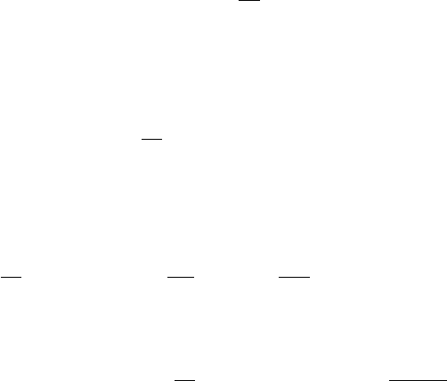
2. (a) Starting from the initial point (0, −2) and following the direction markers we get
the curve shown in Fig. 1–B on page 30.
Thus, the solution curve to the initial value problem dy/dx = 2x + y, y(0) = −2,
is the line with slope
dy
dx
(0) = (2x + y)|
x=0
= y(0) = −2
and y-intercept y(0) = −2. Using the slope-intercept form of an equation of a line,
we get y = −2x −2.
22

Exercises 1.3
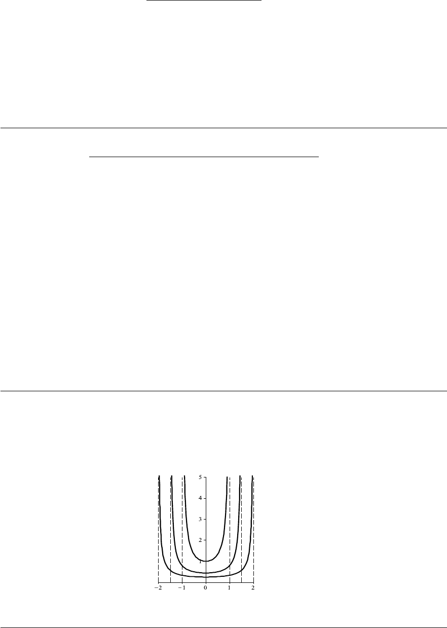
(b) This time, we start from the point (−1, 3) and obtain the curve shown in Fig. 1–C
on page 30.
(c) From Fig. 1–C, we conclude that
lim
x→∞
y(x) = ∞, lim
x→−∞
y(x) = ∞.
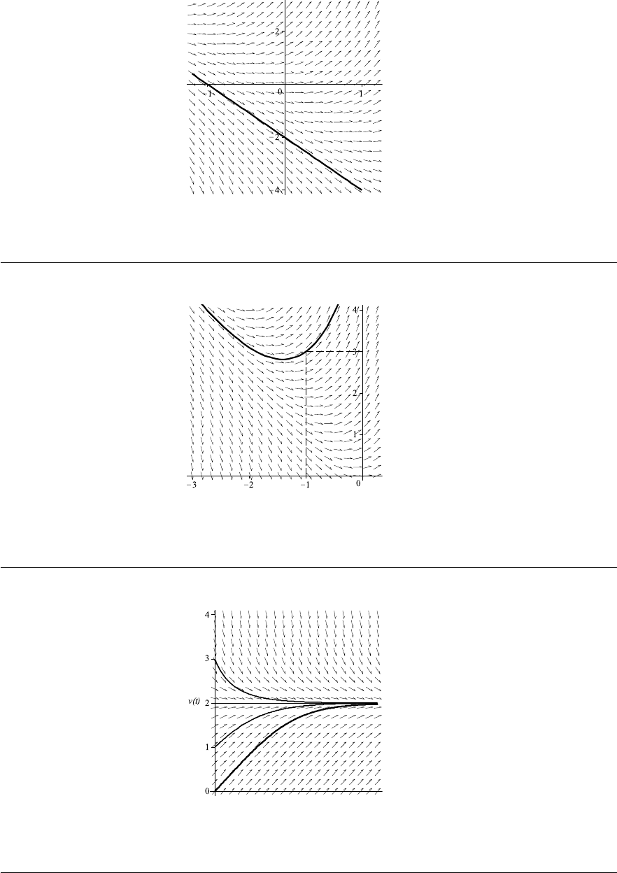
4. The direction field and the solution curve satisfying the given initial conditions are
sketched in Fig. 1–D on page 30. From this figure we find that the terminal velocity is
lim
t→∞
v(t) = 2.
6. (a) The slope of the solution curve to the differential equation y
0
= x + sin y at a point
(x, y) is given by y
0
. Therefore the slope at (1, π/2) is equal to
dy
dx
x=1
= (x + sin y)|
x=1
= 1 + sin
π
2
= 2.
(b) The solution curve is increasing if the slope of the curve is greater than zero. From
the part (a), we know that the slope is x + sin y. The function sin y has values
ranging from −1 to 1; therefore if x is greater than 1 then the slope will always
have a value greater than zero. This tells us that the solution curve is increasing.
(c) The second derivative of every solution can be determined by differentiating both
sides of the original equation, y
0
= x + sin y. Thus
d
dx
dy
dx
=
d
dx
(x + sin y) ⇒
d
2
y
dx
2
= 1 + (cos y)
dy
dx
(chain rule)
= 1 + (cos y)(x + sin y)
= 1 + x cos y + sin y cos y = 1 + x cos y +
1
2
sin 2y .
(d) Relative minima occur when the first derivative, y
0
, is equal to zero and the second
derivative, y
00
, is positive (Second Derivative Test). The value of the first derivative
at the point (0, 0) is given by
dy
dx
= 0 + sin 0 = 0.
This tells us that the solution has a critical point at the point (0, 0). Using the
second derivative found in part (c) we have
d
2
y
dx
2
= 1 + 0 · cos 0 +
1
2
sin 0 = 1.
23

Chapter 1
This tells us that the point (0, 0) is a point of relative minimum.
8. (a) For this particle, we have x(2) = 1, and so the velocity
v(2) =
dx
dt
t=2
= t
3
− x
3
t=2
= 2
3
− x(2)
3
= 7.
(b) Differentiating the given equation yields
d
2
x
dt
2
=
d
dt
dx
dt
=
d
dt
t
3
− x
3
= 3t
2
− 3x
2
dx
dt
= 3t
2
− 3x
2
t
3
− x
3
= 3t
2
− 3t
3
x
2
+ 3x
5
.
(c) The function u
3
is an increasing function. Therefore, as long as x(t) < t, x(t)
3
< t
3
and
dx
dt
= t
3
− x(t)
3
> 0
meaning that x(t) increases. At the initial point t
0
= 2.5 we have x(t
0
) = 2 < t
0
.
Therefore, x(t) cannot take values smaller than 2.5, and the answer is “no”.
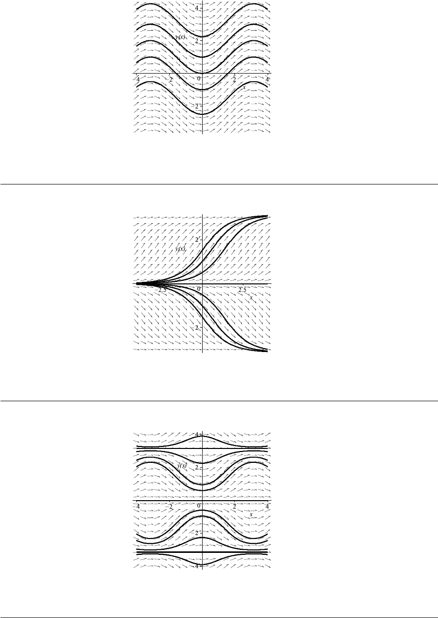
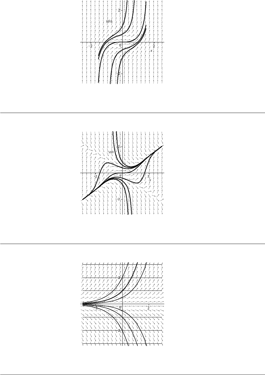
10. Direction fields and some solution curves to differential equations given in (a)–(e) are
shown in Fig. 1–E through Fig. 1–I on pages 31–32.
(a) y
0
= sin x.
(b) y
0
= sin y.
(c) y
0
= sin x sin y.
(d) y
0
= x
2
+ 2y
2
.
(e) y
0
= x
2
− 2y
2
.
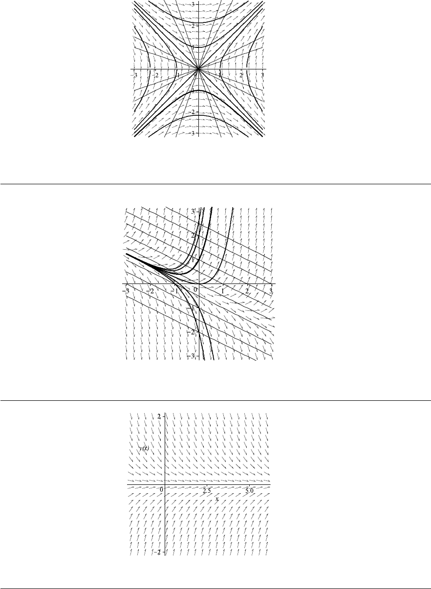
12. The isoclines satisfy the equation f(x, y) = y = c, i.e., they are horizontal lines shown in
Fig. 1–J, page 32, along with solution curves. The curve, satisfying the initial condition,
is shown in bold.
14. Here, f(x, y) = x/y, and so the isoclines are defined by
x
y
= c ⇒ y =
1
c
x.
These are lines passing through the origin and having slope 1/c. See Fig. 1–K on
page 33.
24
Exercises 1.4
16. The relation x + 2y = c yields y = (c −x)/2. Therefore, the isoclines are lines with slope
−1/2 and y-intercept c/2. See Fig. 1–L on page 33.
18. The direction field for this equation is shown in Fig. 1–M on page 33. From this picture
we conclude that any solution y(x) approaches zero, as x → +∞.
EXERCISES 1.4: The Approximation Method of Euler
2. In this problem, x
0
= 0, y
0
= 4, h = 0.1, and f(x, y) = −x/y. Thus, the recursive
formulas given in equations (2) and (3) of the text become
x
n+1
= x
n
+ h = x
n
+ 0.1 ,
y
n+1
= y
n
+ hf(x
n
, y
n
) = y
n
+ 0.1
−
x
n
y
n
, n = 0, 1, 2, . . . .
To find an approximation for the solution at the point x
1
= x
0
+ 0.1 = 0.1, we let n = 0
in the last recursive formula to find
y
1
= y
0
+ 0.1
−
x
0
y
0
= 4 + 0.1(0) = 4.
To approximate the value of the solution at the point x
2
= x
1
+ 0.1 = 0.2, we let n = 1
in the last recursive formula to obtain
y
2
= y
1
+ 0.1
−
x
1
y
1
= 4 + 0.1
−
0.1
4
= 4 −
1
400
= 3.9975 ≈ 3.998 .
Continuing in this way we find
x
3
= x
2
+ 0.1 = 0.3 , y
3
= y
2
+ 0.1
−
x
2
y
2
= 3.9975 + 0.1
−
0.2
3.9975
≈ 3.992 ,
x
4
= 0.4 , y
4
≈ 3.985 ,
x
5
= 0.5 , y
5
≈ 3.975 ,
where all of the answers have been rounded off to three decimal places.
4. Here x
0
= 0, y
0
= 1, and f(x, y) = x + y. So,
x
n+1
= x
n
+ h = x
n
+ 0.1 ,
y
n+1
= y
n
+ hf(x
n
, y
n
) = y
n
+ 0.1 (x
n
+ y
n
) , n = 0, 1, 2, . . . .
Letting n = 0, 1, 2, 3, and 4, we recursively find
x
1
= x
0
+ h = 0.1 , y
1
= y
0
+ 0.1 (x
0
+ y
0
) = 1 + 0.1(0 + 1) = 1.1 ,
25
Chapter 1
x
2
= x
1
+ h = 0.2 , y
2
= y
1
+ 0.1 (x
1
+ y
1
) = 1.1 + 0.1(0.1 + 1.1) = 1.22 ,
x
3
= x
2
+ h = 0.3 , y
3
= y
2
+ 0.1 (x
2
+ y
2
) = 1.22 + 0.1(0.2 + 1.22) = 1.362 ,
x
4
= x
3
+ h = 0.4 , y
4
= y
3
+ 0.1 (x
3
+ y
3
) = 1.362 + 0.1(0.3 + 1.362) = 1.528 ,
x
5
= x
4
+ h = 0.5 , y
5
= y
4
+ 0.1 (x
4
+ y
4
) = 1.5282 + 0.1(0.4 + 1.5282) = 1.721 ,
where all of the answers have been rounded off to three decimal places.
6. In this problem, x
0
= 1, y
0
= 0, and f(x, y) = x −y
2
. So, we let n = 0, 1, 2, 3, and 4, in
the recursive formulas and find
x
1
= x
0
+ h = 1.1 , y
1
= y
0
+ 0.1
x
0
− y
2
0
= 0 + 0.1(1 − 0
2
) = 0.1 ,
x
2
= x
1
+ h = 1.2 , y
2
= y
1
+ 0.1
x
1
− y
2
1
= 0.1 + 0.1(1.1 − 0.1
2
) = 0.209 ,
x
3
= x
2
+ h = 1.3 , y
3
= y
2
+ 0.1
x
2
− y
2
2
= 0.209 + 0.1(1.2 − 0.209
2
) = 0.325 ,
x
4
= x
3
+ h = 1.4 , y
4
= y
3
+ 0.1
x
3
− y
2
3
= 0.325 + 0.1(1.3 − 0.325
2
) = 0.444 ,
x
5
= x
4
+ h = 1.5 , y
5
= y
4
+ 0.1
x
4
− y
2
4
= 0.444 + 0.1(1.4 − 0.444
2
) = 0.564 ,
where all of the answers have been rounded off to three decimal places.
8. The initial values are x
0
= y
0
= 0, f(x, y) = 1 −sin y. If number of steps is N, then the
step h = (π − x
0
)/N = π/N.
For N = 1, h = π,
x
1
= x
0
+ h = π, y
1
= y
0
+ h(1 − sin y
0
) = π ≈ 3.1416 .
For N = 2, h = π/2,
x
1
= x
0
+ π/2 = π/2, y
1
= y
0
+ h(1 − sin y
0
) = π/2 ≈ 1.571 ,
x
2
= x
1
+ π/2 = π, y
2
= y
1
+ h(1 − sin y
1
) = π/2 ≈ 1.571 .
We continue with N = 4 and 8, and fill in Table 1 on page 28, where the approximations
to φ(π) are rounded to three decimal places.
10. We have x
0
= y(0) = 0, h = 0.1. With this step size, we need (1 − 0)/0.1 = 10 s teps to
approximate the solution on [0, 1]. The results of computation are given in Table 1 on
page 28.
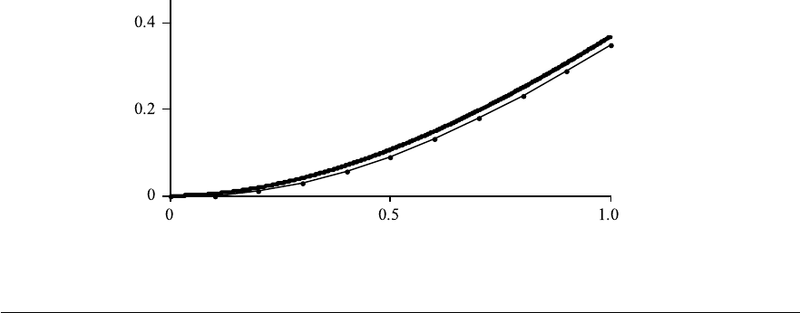
26

Exercises 1.4
Next we check that y = e
−x
+ x − 1 is the actual solution to the given initial value
problem.
y
0
=
e
−x
+ x − 1
0
= −e
−x
+ 1 = x −
e
−x
+ x − 1
= x − y,
y(0) =
e
−x
+ x − 1
x=0
= e
0
+ 0 − 1 = 0.
Thus, it is the solution.
The solution curve y = e
−x
+ x − 1 and the polygonal line approximation using data
from Table 1 are shown in Fig. 1–N, page 34.
12. Here, x
0
= 0, y
0
= 1, f(x, y) = y. With h = 1/n, the recursive formula (3) of the text
yields
y(1) = y
n
= y
n−1
+
y
n−1
n
= y
n−1
1 +
1
n
=
y
n−2
1 +
1
n
1 +
1
n
= y
n−2
1 +
1
n
2
= . . . = y
0
1 +
1
n
n
=
1 +
1
n
n
.
14. Computation results are given in Table 1 on page 29.
16. For this problem notice that the independent variable is t and the dependent variable is
T . Hence, in the recursive formulas for Euler’s method, t will take the place of x and
T will take the place of y. Also we see that h = 0.1 and f(t, T ) = K (M
4
− T
4
), where
K = 40
−4
and M = 70. Therefore, the recursive formulas given in equations (2) and (3)
of the text become
t
n+1
= t
n
+ 0.1 ,
T
n+1
= T
n
+ hf (t
n
, T
n
) = T
n
+ 0.1
40
−4
70
4
− T
4
n
, n = 0, 1, 2, . . . .
From the initial condition T (0) = 100 we see that t
0
= 0 and T
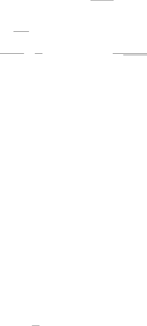
0
= 100. Therefore, for
n = 0, we have
t
1
= t
0
+ 0.1 = 0 + 0.1 = 0.1 ,
T
1
= T
0
+ 0.1(40
−4
)(70
4
− T
4
0
) = 100 + 0.1(40
−4
)(70
4
− 100
4
) ≈ 97.0316,
where we have rounded off to four decimal places.
For n = 1,
t
2
= t
1
+ 0.1 = 0.1 + 0.1 = 0.2 ,
27

Chapter 1
T
2
= T
1
+ 0.1(40
−4
)(70
4
− T
4
1
) = 97.0316 + 0.1(40
−4
)(70
4
− 97.0316
4
) ≈ 94.5068.
By continuing this way, we fill in Table 1 on page 29. From this table we see that
T (1) = T (t
10
) ≈ T
10
= 82.694 ,
T (2) = T (t
20
) ≈ T
20
= 76.446 ,
where we have rounded to three decimal places.
TABLES
N
N
N h
h
h φ
φ
φ(π
π
π)
1 π 3.142
2 π/2 1.571
4 π/4 1.207
8 π/8 1.148
Table 1–A: Euler’s approximations to y
0
= 1 − sin y, y(0) = 0, with N steps.
n
n
n x
x
x
n
n
n
y
y
y
n
n
n
n
n
n x
x
x
n
n
n
y
y
y
n
n
n
0 0 0 6 0.6 0.131
1 0.1 0 7 0.7 0.178
2 0.2 0.01 8 0.8 0.230
3 0.3 0.029 9 0.9 0.287
4 0.4 0.056 10 1.0 0.349
5 0.5 0.091
Table 1–B: Euler’s approximations to y
0
= x − y, y(0) = 0, on [0, 1] with h = 0.1.
28
Figures
h
h
h y
y
y(2)
0.5 24.8438
0.1 ≈ 6.4 · 10
176
0.05 ≈ 1.9 · 10
114571
0.01 > 10
10
30
Table 1–C: Euler’s method approximations of y(2) for y
0
= 2xy
2
, y(0) = 1.
n
n
n t
t
t
n
n
n
T
T
T
n
n
n
n
n
n t
t
t
n
n
n
T
T
T
n
n
n
1 0.1 97.0316 11 1.1 81.8049
2 0.2 94.5068 12 1.2 80.9934
3 0.3 92.3286 13 1.3 80.2504
4 0.4 90.4279 14 1.4 79.5681
5 0.5 88.7538 15 1.5 78.9403
6 0.6 87.2678 16 1.6 78.3613
7 0.7 85.9402 17 1.7 77.8263
8 0.8 84.7472 18 1.8 77.3311
9 0.9 83.6702 19 1.9 76.8721
10 1.0 82.6936 20 2.0 76.4459
Table 1–D: Euler’s approximations to the solution of T
0
= K (M
4
− T
4
), T (0) = 100,
with K = 40
−4
, M = 70, and h = 0.1.
FIGURES
Figure 1–A: Integral curves in Problem 18.
29
Chapter 1
Figure 1–B: The solution curve in Problem 2(a).
Figure 1–C: The solution curve in Problem 2(b).
Figure 1–D: The direction field and solution curves in Problem 4.
30
Figures
Figure 1–E: The direction field and solution curves in Problem 10(a).
Figure 1–F: The direction field and solution curves in Problem 10(b).
Figure 1–G: The direction field and solution curves in Problem 10(c).
31
Chapter 1
Figure 1–H: The direction field and solution curves in Problem 10(d).
Figure 1–I: The direction field and solution curves in Problem 10(e).
Figure 1–J: The isoclines and solution curves in Problem 12.
32
Figures
Figure 1–K: The isoclines and solution curves in Problem 14.
Figure 1–L: The isoclines and solution curves in Problem 16.
Figure 1–M: The direction field in Problem 18.
33
Chapter 1
Figure 1–N: Euler’s method approximations to y = e
−x
+x−1 on [0, 1] with h = 0.1.
34

CHAPTER 2: First Order Differential Equations
EXERCISES 2.2: Separable Equations
2. This equation is not separable because sin(x + y) cannot be expressed as a product
g(x)p(y).
4. This equation is separable because
ds
dt
= t ln
s
2t
+ 8t
2
= t(2t) ln |s| + 8t
2
= 2t
2
(ln |s| + 4).
6. Writing the equation in the form
dy
dx
=
2x
xy
2
+ 3y
2
=
2x
(x + 3)y
2
=
2x
x + 3
·
1
y
2
,
we see that the equation is separable.
8. Multiplying both sides of the equation by y
3
dx and integrating yields
y
3
dy =
dx
x
⇒
Z
y
3
dy =
Z
dx
x
⇒
1
4
y
4
= x ln |x| + C
1
⇒ y
4
= 4 ln |x| + C ⇒ y = ±
4
p
4 ln |x| + C ,
where C := 4C
1
is an arbitrary constant.
10. To separate variables, we divide the equation by x and multiply by dt. Integrating yields
dx
x
= 3t
2
dt ⇒ ln |x| = t
3
+ C
1
⇒ |x| = e
t
3
+C
1
= e
C
1
e
t
3
⇒ |x| = C
2
e
t
3
⇒ x = ±C
2
e
t
3
= Ce
t
3
,
where C
1
is an arbitrary constant and, therefore, C
2
:= e
C
1
is an arbitrary positive
constant, C = ±C
2
is any nonzero constant. Separating variables, we lost a solution
x ≡ 0, which can be included in the above formula by taking C = 0. Thus, x = Ce
t
3
, C
– arbitrary constant, is a general solution.
35
Chapter 2
12. We have
3vdv
1 − 4v
2
=
dx
x
⇒
Z
3vdv
1 − 4v
2
=
Z
dx
x
⇒ −
3
8
Z
du
u
=
Z
dx
x
u = 1 −4v
2
, du = −8vdv
⇒ −
3
8
ln
1 − 4v
2
= ln |x| + C
1
⇒ 1 − 4v
2
= ±exp
−
8
3
ln |x| + C
1
= Cx
−8/3
,
where C = ±e
C
1
is any nonzero constant. Separating variables, we lost constant solutions
satisfying
1 − 4v
2
= 0 ⇒ v = ±
1
2
,
which can be included in the above formula by letting C = 0. Thus,
v = ±
√
1 − Cx
−8/3
2
, C arbitrary,
is a general solution to the given equation.
14. Separating variables, we get
dy
1 + y
2
= 3x
2
dx ⇒
Z
dy
1 + y
2
=
Z
3x
2
dx
⇒ arctan y = x
3
+ C ⇒ y = tan
x
3
+ C
,
where C is any constant. Since 1 + y
2
6= 0, we did not lose any solution.
16. We rewrite the equation in the form
x(1 + y
2
)dx + e
x
2
ydy = 0,
separate variables, and integrate.
e
−x
2
xdx = −
ydy
1 + y
2
⇒
Z
e
−x
2
xdx = −
Z
ydy
1 + y
2
⇒
Z
e
−u
du = −
dv
v
u = x
2
, v = 1 + y
2
⇒ −e
−u
= −ln |v| + C ⇒ ln
1 + y
2
− e
−x
2
= C
is an implicit solution to the given equation. Solving for y yields
y = ±
p
C
1
exp [exp (−x
2
)] − 1,
where C
1
= e
C
is any positive constant,
36
Exercises 2.2
18. Separating variables yields
dy
1 + y
2
= tan xdx ⇒
Z
dy
1 + y
2
=
Z
tan xdx ⇒ arctan y = −ln |cos x| + C.
Since y(0) =
√
3, we have
arctan
√
3 = −ln cos 0 + C = C ⇒ C =
π
3
.
Therefore,
arctan y = −ln |cos x| +
π
3
⇒ y = tan
−ln |cos x| +
π
3
is the solution to the given initial value problem.
20. Separating variables and integrating, we get
Z
(2y + 1)dy =
Z
3x
2
+ 4x + 2
dx ⇒ y
2
+ y = x
3
+ 2x
2
+ 2x + C.
Since y(0) = −1, substitution yields
(−1)
2
+ (−1) = (0)
3
+ 2(0)
2
+ 2(0) + C ⇒ C = 0,
and the solution is given, implicitly, by y
2
+ y = x
3
+ 2x
2
+ 2x or, explicitly, by
y = −
1
2
−
r
1
4
+ x
3
+ 2x
2
+ 2x.
(Solving for y, we used the initial condition.)
22. Writing 2ydy = −x
2
dx and integrating, we find
y
2
= −
x
3
3
+ C.
With y(0) = 2,
(2)
2
= −
(0)
3
3
+ C ⇒ C = 4,
and so
y
2
= −
x
3
3
+ 4 ⇒ y =
r
−
x
3
3
+ 4.
We note that, taking the square root, we chose the positive sign because y(0) > 0.
37
Chapter 2
24. For a general solution, we separate variables and integrate.
Z
e
2y
dy =
Z
8x
3
dx ⇒
e
2y
2
= 2x
4
+ C
1
⇒ e
2y
= 4x
4
+ C.
We substitute now the initial condition, y(1) = 0, and obtain
1 = 4 + C ⇒ C = −3.
Hence, the answer is given by
e
2y
= 4x
4
− 3 ⇒ y =
1
2
ln
4x
4
− 3
.
26. We separate variables and obtain
Z
dy
√
y
= −
Z
dx
1 + x
⇒ 2
√
y = −ln |1 + x| + C = −ln(1 + x) + C,
because at initial point, x = 0, 1 + x > 0. Using the fact that y(0) = 1, we find C.
2 = 0 + C ⇒ C = 2,
and so y = [2 − ln(1 + x)]
2
/4 is the answer.
28. We have
dy
dt
= 2y(1 −t) ⇒
dy
y
= 2(1 − t)dt ⇒ ln |y| = −(t − 1)
2
+ C
⇒ y = ±e
C
e
−(t−1)
2
= C
1
e
−(t−1)
2
,
where C
1
6= 0 is any constant. Separating variables, we lost the solution y ≡ 0. So, a
general solution to the given equation is
y = C
2
e
−(t−1)
2
, C
2
is any.
Substituting t = 0 and y = 3, we find
3 = C
2
e
−1
⇒ C
2
= 3e ⇒ y = 3e
1−(t−1)
2
= 3e
2t−t
2
.
The graph of this function is given in Fig. 2–A on page 71.
Since y(t) > 0 for any t, from the given equation we have y
0
(t) > 0 for t < 1 and y
0
(t) < 0
for t > 1. Thus t = 1 is the point of absolute maximum with y
max
= y(1) = 3e.
38

Exercises 2.2
30. (a) Dividing by (y + 1)
2/3
, multiplying by dx, and integrating, we obtain
Z
dy
(y + 1)
2/3
=
Z
(x − 3)dx ⇒ 3(y + 1)
1/3
=
x
2
2
− 3x + C
⇒ y = −1 +
x
2
6
− x + C
1
3
.
(b) Substituting y ≡ −1 into the original equation yields
d(−1)
dx
= (x − 3)(−1 + 1)
2/3
= 0,
and so the equation is satisfied.
(c) For y ≡ −1 for the solution in part (a), we must have
x
2
6
− x + C
1
3
≡ 0 ⇔
x
2
6
− x + C
1
≡ 0,
which is impossible since a quadratic polynomial has at most two zeros.
32. (a) The direction field of the given differential equation is shown in Fig. 2–B, page 72.
Using this picture we predict that lim
x→∞
φ(x) = 1.
(b) In notation of Section 1.4, we have x
0
= 0, y
0
= 1.5, f(x, y) = y
2
− 3y + 2, and
h = 0.1. With this step size, we need (1 − 0)/0.1 = 10 steps to approximate φ(1).
The results of computation are given in Table 2 on page 71. From this table we
conclude that φ(1) ≈ 1.26660 .
(c) Separating variables and integrating, we obtain
dy
y
2
− 3y + 2
= dx ⇒
Z
dy
y
2
− 3y + 2
=
Z
dx ⇒ ln
y − 2
y − 1
= x + C ,
where we have used a partial fractions decomposition
1
y
2
− 3y + 2
=
1
y − 2
−
1
y − 1
to evaluate the integral. The initial condition, y(0) = 1.5 , implies that C = 0, and
so
ln
y − 2
y − 1
= x ⇒
y − 2
y − 1
= e
x
⇒
y − 2
y − 1
= −e
x
.
(We have chosen the negative sign because of the initial condition.) Solving for y
yields
y = φ(x) =
e
x
+ 2
e
x
+ 1
The graph of this solution is shown in Fig. 2–B on page 72.
39

Chapter 2
(d) We find
φ(1) =
e + 2
e + 1
≈ 1.26894 .
Thus, the approximate value φ(1) ≈ 1.26660 found in part (b) differs from the
actual value by less than 0.003 .
(e) We find the limit of φ(x) at infinity writing
lim
x→∞
e
x
+ 2
e
x
+ 1
= lim
x→∞
1 +
1
e
x
+ 1
= 1 ,
which confirms our guess in part (a).
34. (a) Separating variables and integrating, we get
dT
T − M
= −kdt ⇒
Z
dT
T − M
= −
Z
kdt ⇒ ln |T − M| = −kt + C
1
⇒ |T − M| = e
C
1
e
−kt
⇒ T − M = ±e
C
1
e
−kt
= Ce
−kt
,
where C is any nonzero constant. We can include the lost solution T ≡ M into this
formula by letting C = 0. Thus, a general solution to the equation is
T = M + Ce
−kt
.
(b) Given that M = 70
◦
, T (0) = 100
◦
, T (6) = 80
◦
, we form a system to determine C
and k.
(
100 = 70 + C
80 = 70 + Ce
−6k
⇒
(
C = 30
k = −(1/6) ln[(80 − 70)/30] = (1/6) ln 3.
Therefore,
T = 70 + 30e
−(t ln 3)/6
= 70 + (30)3
−t/6
,
and after 20 min the reading is
T (20) = 70 + (30)3
−20/6
≈ 70.77
◦
.
36. A general solution to the cooling equation found in Problem 34, that is, T = M + Ce
−kt
.
Since T (0) = 100
◦
, T (5) = 80
◦
, and T (10) = 65
◦
, we determine M, C, and k from the
system
M + C = 100
M + Ce
−5k
= 80
M + Ce
−10k
= 65
⇒
(
C(1 −e
−5k
) = 20
Ce
−5k
(1 − e
−5k
) = 15
⇒ e
−5k
= 3/4.
40

Exercises 2.3
To find M, we can now use the first two equations in the above s ystem.
(
M + C = 100
M + (3/4)C = 80
⇒ M = 20.
38. With m = 10, g = 9.81, and k = 5, the equation becomes
100
dv
dt
= 100(9.81) − 5v ⇒ 20
dv
dt
= 196.2 − v.
Separating variables and integrating yields
Z
dv
v − 196.2
= −
1
20
Z
dt ⇒ ln |v − 196.2| = −
t
20
+ C
1
⇒ v = 196.2 + Ce
−t/20
,
where C is an arbitrary nonzero constant. With C = 0, this formula also gives the (lost)
constant solution v = 196.2. From the initial condition, v(0) = 10, we find C.
196.2 + C = 10 ⇒ C = −186.2 ⇒ v(t) = 196.2 −186.2e
−t/20
.
The terminal velocity of the object can be found by letting t → ∞.
v
∞
= lim
t→∞
196.2 − 186.2e
−t/20
= 196.2 (m/sec).
EXERCISES 2.3: Linear Equations
2. Neither.
4. Linear.
6. Linear.
8. Writing the equation in standard form,
dy
dx
−
y
x
= 2x + 1,
we see that
P (x) = −
1
x
⇒ µ(x) = exp
Z
−
1
x
dx
= exp (−ln x) =
1
x
.
Multiplying the given equation by µ(x), we get
d
dx
y
x
= 2 +
1
x
⇒ y = x
Z
2 +
1
x
dx = x (2x + ln |x| + C) .
41

Chapter 2
10. From the standard form of the given equation,
dy
dx
+
2
x
y = x
−4
,
we find that
µ(x) = exp
Z
(2/x)dx
= exp (2 ln x) = x
2
⇒
d
dx
x
2
y
= x
−2
⇒ y = x
−2
Z
x
−2
dx = x
−2
−x
−1
+ C
=
Cx −1
x
3
.
12. Here, P (x) = 4, Q(x) = x
2
e
−4x
. So, µ(x) = e
4x
and
d
dx
e
4x
y
= x
2
⇒ y = e
−4x
Z
x
2
dx = e
−4x
x
3
3
+ C
.
14. We divide the equation by x to get to get its standard form.
dy
dx
+
3
x
y = x
2
− 2x + 4.
Thus, P (x) = 3/x, Q(x) = x
2
− 2x + 4,
µ(x) = exp
Z
3
x
dx
= x
3
⇒ x
3
y =
Z
x
3
x
2
− 2x + 4
dx =
x
6
6
−
2x
5
5
+ x
4
+ C
⇒ y =
x
3
6
−
2x
2
5
+ x + Cx
−3
.
16. We divide by x
2
+ 1 both sides of the given equation to get its standard form,
dy
dx
+
4x
x
2
+ 1
y =
x
2
+ 2x − 1
x
2
+ 1
.
Thus, P (x) = (4x)/(x
2
+ 1), Q(x) = (x
2
+ 2x − 1)/(x
2
+ 1),
µ(x) = exp
Z
4x
x
2
+ 1
dx
= exp
2 ln(x
2
+ 1)
= (x
2
+ 1)
2
⇒ (x
2
+ 1)
2
y =
Z
(x
2
+ 1)(x
2
+ 2x − 1)dx =
x
5
5
+
x
4
2
+ x
2
− x + C
⇒ y =
x
5
5
+
x
4
2
+ x
2
− x + C
x
2
+ 1
−2
.
42

Exercises 2.3
18. Since µ(x) = exp
R
4dx
= e
4x
, we have
d
dx
e
4x
y
= e
4x
e
−x
= e
3x
⇒ y = e
−4x
Z
e
3x
dx =
e
−x
3
+ Ce
−4x
.
Substituting the initial condition, y = 4/3 at x = 0, yields
4
3
=
1
3
+ C ⇒ C = 1,
and so y = e
−x
/3 + e
−4x
is the solution to the given initial value problem.
20. We have
µ(x) = exp
Z
3dx
x
= exp (3 ln x) = x
3
⇒ x
3
y =
Z
x
3
(3x − 2) dx =
3x
5
5
−
x
4
2
+ C
⇒ y =
3x
2
5
−
x
2
+ Cx
−3
.
With y(1) = 1,
1 = y(1) =
3
5
−
1
2
+ C ⇒ C =
9
10
⇒ y =
3x
2
5
−
x
2
+
9
10x
3
.
22. From the standard form of this equation,
dy
dx
+ y cot x = x,
we find
µ(x) = exp
Z
cot x dx
= exp (ln sin x) = sin x.
(Alternatively, one can notice that the left-hand side of the original equation is the
derivative of the product y sin x.) So, using integration by parts, we obtain
y sin x =
Z
x sin x dx = −x cos x + sin x + C
⇒ y = −x cot x + 1 + C csc x.
We find C using the initial condition y(π/2) = 2:
2 = −
π
2
cot
π
2
+ 1 + C csc
π
2
= 1 + C ⇒ C = 1,
and the solution is given by
y = −x cot x + 1 + csc x.
43

Chapter 2
24. (a) The equation (12) on of the text becomes
dy
dt
+ 20y = 50e−10t ⇒ µ(t) = e
20t
⇒ y = e
−20t
Z
50e
10t
dt = 5e
−10t
+ Ce
−20t
.
Since y(0) = 40, we have
40 = 5 + C ⇒ C = 35 ⇒ y = 5e
−10t
+ 35e
−20t
.
The term 5e
−10t
will eventually dominate.
(b) This time, the equation (12) has the form
dy
dt
+ 10y = 50e−10t ⇒ µ(t) = e
10t
⇒ y = e
−10t
Z
50dt = e
−10t
(50t + C).
Substituting the initial condition yields
40 = y(0) = C ⇒ y = e
−10t
(50t + 40).
26. Here
P (x) =
sin x cos x
1 + sin
2
x
⇒ µ(x) = exp
Z
sin x cos x dx
1 + sin
2
x
= exp
1
2
ln
1 + sin
2
x
=
p
1 + sin
2
x.
Thus,
y
p
1 + sin
2
x =
x
Z
0
p
1 + sin
2
tdt ⇒ y = (1 + sin
2
x)
−1/2
x
Z
0
(1 + sin
2
t)
1/2
dt
and
y(1) = (1 + sin
2
1)
−1/2
1
Z
0
(1 + sin
2
t)
1/2
dt.
We now use the Simpson’s Rule to find that y(1) ≈ 0.860.
28. (a) Substituting y = e
−x
into the equation (16) yields
d(e
−x
)
dx
+ e
−x
= −e
−x
+ e
−x
= 0.
44
Exercises 2.3
So, y = e
−x
is a solution to (16).
The function y = x
−1
is a solution to (17) because
d(x
−1
)
dx
+ (x
−1
)
2
= (−1)x
−2
+ x
−2
= 0.
(b) For any constant C,
d(Ce
−x
)
dx
+ Ce
−x
= −Ce
−x
+ Ce
−x
= 0.
Thus y = Ce
−x
is a solution to (16).
Substituting y = Cx
−1
into (17), we obtain
d(Cx
−1
)
dx
+ (Cx
−1
)
2
= (−C)x
−2
+ C
2
x
−2
= C(C − 1)x
−2
,
and so we must have C(C − 1) = 0 in order that y = Cx
−1
is a solution to (17).
Thus, either C = 0 or C = 1.
(c) For the function y = C ˆy, one has
d(C ˆy)
dx
+ P (x) (C ˆy) = C
dˆy
dx
+ C (P (x)ˆy) = C
dˆy
dx
+ P (x)ˆy
= 0
if ˆy is a solution to y
0
+ P (x)y = 0.
30. (a) Multiplying both sides of (18) by y
2
, we get
y
2
dy
dx
+ 2y
3
= x.
If v = y
3
, then v
0
= 3y
2
y
0
. Thus, y
2
y
0
= v
0
/3, and we have
1
3
dv
dx
+ 2v = x,
which is equivalent to (19).
(b) The equation (19) is linear with P (x) = 6 and Q(x) = 3x. So,
µ(x) = exp
Z
6dx
= e
6x
⇒ v(x) = e
−6x
Z
(3xe
6x
)dx =
e
−6x
2
xe
6x
−
Z
e
6x
dx
=
e
−6x
2
xe
6x
−
e
6x
6
+ C
1
=
x
2
−
1
12
+ Ce
−6x
,
where C = C
1
/2 is an arbitrary constant. The back substitution yields
y =
3
r
x
2
−
1
12
+ Ce
−6x
.
45

Chapter 2
32. In the given equation, P (x) = 2, which implies that µ(x) = e
2x
. Following guidelines,
first we solve the equation on [0, 3]. On this interval, Q(x) ≡ 2. Therefore,
y
1
(x) = e
−2x
Z
(2)e
2x
dx = 1 + C
1
e
−2x
.
Since y
1
(0) = 0, we get
1 + C
1
e
0
= 0 ⇒ C
1
= −1 ⇒ y
1
(x) = 1 −e
−2x
.
For x > 3, Q(x) = −2 and so
y
2
(x) = e
−2x
Z
(−2)e
2x
dx = −1 + C
2
e
−2x
.
We now choose C
2
so that
y
2
(3) = y
1
(3) = 1 −e
−6
⇒ −1 + C
2
e
−6
= 1 − e
−6
⇒ C
2
= 2e
6
− 1.
Therefore, y
2
(x) = −1 + (2e
6
− 1)e
−2x
, and the continuous solution to the given initial
value problem on [0, ∞) is
y(x) =
(
1 − e
−2x
, 0 ≤ x ≤ 3,
−1 + (2e
6
− 1)e
−2x
, x > 3.
The graph of this function is shown in Fig. 2–C, page 72.
34. (a) Since P (x) is continuous on (a, b), its antiderivatives given by
R
P (x)dx are con-
tinuously differentiable, and therefore continuous, functions on (a, b). Since the
function e
x
is continuous on (−∞, ∞), composite functions µ(x) = e
R
P (x)dx
are
continuous on (a, b). The range of the exponential f unction is (0, ∞). This implies
that µ(x) is positive with any choice of the integration constant. Using the chain
rule, we conclude that
dµ(x)
dx
= e
R
P (x)dx
d
dx
Z
P (x)dx
= µ(x)P (x)
for any x on (a, b).
(b) Differentiating (8), we apply the product rule and obtain
dy
dx
= −µ
−2
µ
0
Z
µQ dx + C
+ µ
−1
µQ = −µ
−1
P
Z
µQ dx + C
+ Q ,
and so
dy
dx
+ P y =
−µ
−1
P
Z
µQ dx + C
+ Q
+ P
µ
−1
Z
µQ dx + C
= Q .
46

Exercises 2.3
(c) Suggested choice of the antiderivative and the constant C yields
y(x
0
) = µ(x)
−1
x
Z
x
0
µQdx + y
0
µ(x
0
)
x=x
0
= µ(x
0
)
−1
y
0
µ(x
0
) = y
0
.
(d) We assume that y(x) is a solution to the initial value problem (15). Since µ(x) is a
continuous positive function on (a, b), the equation (5) is equivalent to (4). Since,
from the part (a), the left-hand side of (5) is the derivative of the product µ(x)y(x),
this function must be an antiderivative of the right-hand side, which is µ(x)Q(x).
Thus, we come up with (8), where the integral means one of the antiderivatives, for
example, the one suggested in the part (c) (which has zero value at x
0
). Substituting
x = x
0
into (8), we conclude that
y
0
= y(x
0
) = µ(x
0
)
−1
Z
µQdx + C
x=x
0
= Cµ(x
0
)
−1
,
and so C = y
0
µ(x
0
) is uniquely defined.
36. (a) If µ(x) = exp
R
P dx
and y
h
(x) = µ(x)
−1
, then
dy
h
dx
= (−1)µ(x)
−2
dµ(x)
dx
= −µ(x)
−2
µ(x)P (x) = −µ(x)
−1
P (x)
and so
dy
h
dx
+ P (x)y
h
= −µ(x)
−1
P (x) + P (x)µ(x)
−1
= 0,
i.e., y
h
is a solution to the equation y
0
+ P y = 0. Now, the formula (8) yields
y = µ(x)
−1
Z
µ(x)Q(x)dx + C
= y
h
(x)v(x) + Cy
h
(x) = y
p
(x) + Cy
h
(x),
where v(x) =
R
µ(x)Q(x)dx.
(b) Separating variables in (22) and integrating, we obtain
dy
y
= −
3dx
x
⇒
Z
dy
y
= −
Z
3dx
x
⇒ ln |y| = −3 ln x + C.
Since we need just one solution y
h
, we take C = 0
ln |y| = −3 ln x ⇒ y = ±x
−3
,
and we choose, say, y
h
= x
−3
.
47

Chapter 2
(c) Substituting y
p
= v(x)y
h
(x) = v(x)x
−3
into (21), we get
dv
dx
y
h
+ v
dy
h
dx
+
3
x
vy
h
=
dv
dx
y
h
+ v
dy
h
dx
+
3
x
y
h
=
dv
dx
y
h
= x
2
.
Therefore, dv/dx = x
2
/y
h
= x
5
.
(d) Integrating yields
v(x) =
Z
x
5
dx =
x
6
6
.
(We have chosen zero integration constant.)
(e) The function
y = Cy
h
+ vy
h
= Cx
−3
+
x
3
6
is a general solution to (21) because
dy
dx
+
3
x
y =
d
dx
Cx
−3
+
x
3
6
+
3
x
Cx
−3
+
x
3
6
=
−3Cx
−4
+
x
2
2
+
3Cx
−4
+
x
2
2
= x
2
.
38. Dividing both sides of (6) by µ and multiplying by dx yields
dµ
µ
= P dx ⇒
Z
dµ
µ
=
Z
P dx
⇒ ln |µ| =
Z
P dx ⇒ µ = ±exp
Z
P dx
.
Choosing the positive sign, we obtain (7).
EXERCISES 2.4: Exact Equations
2. This equation is not separable because the coefficient x
10/3
− 2y cannot be written as a
product f(x)g(y). Writing the equation in the form
x
dy
dx
− 2y = −x
10/3
,
we see that the equation is linear. Since M(x, y) = x
10/3
− 2y, N(x, y) = x,
∂M
∂y
= −2 6=
∂N
∂x
= 1,
and so the equation is not exact.
48

Exercises 2.4
4. First we note that M(x, y) =
p
−2y − y
2
depends only on y and N(x, y) = 3 + 2x − x
2
depends only on x. So, the equation is separable. It is not linear with x as independent
variable because M(x, y) is not a linear function of y. Similarly, it is not linear with y
as independent variable because N(x, y) is not a linear function of x. Computing
∂M
∂y
=
1
2
−2y − y
2
−1/2
(−2 − 2y) = −
1 + y
p
−2y − y
2
,
∂N
∂x
= 2 − 2x,
we see that the equation (5) in Theorem 2 is not satisfied. Therefore, the equation is
not exact.
6. It is separable, linear with x as independent variable, and not exact because
∂M
∂y
= x 6=
∂N
∂x
= 0.
8. Here, M(x, y) = 2x + y cos(xy), N(x, y) = x cos(xy) −2y. Since M(x, y)/N(x, y) cannot
be expressed as a product f(x)g(y), the equation is not separable. We also conclude that
it is not linear because M(x, y)/N(x, y) is not a linear function of y and N(x, y)/M(x, y)
is not a linear function of x. Taking partial derivatives
∂M
∂y
= cos(xy) −xy sin(xy) =
∂N
∂x
,
we see that the equation is exact.
10. In this problem, M(x, y) = 2x + y, N(x, y) = x − 2y. Thus, M
y
= N
x
= 1, and the
equation is exact. We find
F (x, y) =
Z
(2x + y)dx = x
2
+ xy + g(y),
∂F
∂y
= x + g
0
(y) = N (x, y) = x − 2y
⇒ g
0
(y) = −2y ⇒ g(y) =
Z
(−2y)dy = −y
2
⇒ F (x, y) = x
2
+ xy − y
2
,
and so x
2
+ xy − y
2
= C is a general solution.
12. We compute
∂M
∂y
= e
x
cos y =
∂N
∂x
.
49
Chapter 2
Thus, the equation is exact.
F (x, y) =
Z
e
x
sin y − 3x
2
dx = e
x
sin y − x
3
+ g(y),
∂F
∂y
= e
x
cos y + g
0
(y) = e
x
cos y −
1
3
y
−2/3
⇒ g
0
(y) = −
1
3
y
−2/3
⇒ g(y) =
1
3
Z
y
−2/3
dy = y
1/3
.
So, e
x
sin y − x
3
+
3
√
y = C is a general solution.
14. Since M(t, y) = e
t
(y − t), N(t, y) = 1 + e
t
, we find that
∂M
∂y
= e
t
=
∂N
∂t
.
Then
F (t, y) =
Z
(1 + e
t
)dy = (1 + e
t
)y + h(t),
∂F
∂t
= e
t
y + h
0
(t) = e
t
(y − t) ⇒ h0(t) = −te
t
⇒ h(t) = −
Z
te
t
dt = −(t −1)e
t
,
and a general solution is given by
(1 + e
t
)y − (t − 1)e
t
= C ⇒ y =
(t − 1)e
t
+ C
1 + e
t
.
16. Computing
∂M
∂y
=
∂
∂y
ye
xy
− y
−1
= e
xy
+ xye
xy
+ y
−2
,
∂N
∂x
=
∂
∂x
xe
xy
+ xy
−2
= e
xy
+ xye
xy
+ y
−2
,
we see that the equation is exact. Therefore,
F (x, y) =
Z
ye
xy
− y
−1
dx = e
xy
− xy
−1
+ g(y).
So,
∂F
∂y
= xe
xy
+ xy
−2
+ g
0
(y) = N (x, y) ⇒ g
0
(y) = 0.
Thus, g(y) = 0, and the answer is e
xy
− xy
−1
= C.
50

Exercises 2.4
18. Since
∂M
∂y
=
∂N
∂x
= 2y
2
+ sin(x + y),
the equation is exact. We find
F (x, y) =
Z
2x + y
2
− cos(x + y)
dx = x
2
+ xy
2
− sin(x + y) + g(y),
∂F
∂y
= 2xy − cos(x + y) + g
0
(y) = 2xy − cos(x + y) −e
y
⇒ g
0
(y) = −e
y
⇒ g(y) = −e
y
.
Therefore,
F (x, y) = x
2
+ xy
2
− sin(x + y) −e
y
= C
gives a general solution.
20. We find
∂M
∂y
=
∂
∂y
[y cos(xy)] = cos(xy) − xy sin(xy),
∂N
∂x
=
∂
∂x
[x cos(xy)] = cos(xy) − xy sin(xy).
Therefore, the equation is exact and
F (x, y) =
Z
x cos(xy) − y
−1/3
dy = sin(xy) −
3
2
y
2/3
+ h(x)
∂F
∂x
= y cos(xy) + h
0
(x) =
2
√
1 − x
2
+ y cos(xy)
⇒ h
0
(x) =
2
√
1 − x
2
⇒ h(x) = 2 arcsin x,
and a general solution is given by
sin(xy) −
3
2
y
2/3
+ 2 arcsin x = C.
22. In Problem 16, we found that a general solution to this equation is
e
xy
− xy
−1
= C.
Substituting the initial condition, y(1) = 1, yields e − 1 = C. So, the answer is
e
xy
− xy
−1
= e − 1.
51

Chapter 2
24. First, we check the given equation for exactness.
dM
dx
= e
t
=
∂N
∂t
.
So, it is exact. We find
F (t, x) =
Z
e
t
− 1
dx = x
e
t
− 1
+ g(t),
∂F
∂t
= xe
t
+ g
0
(t) = xe
t
+ 1 ⇒ g(t) =
Z
dt = t
⇒ x
e
t
− 1
+ t = C
is a general solution. With x(1) = 1, we get
(1) (e − 1) + 1 = C ⇒ C = e,
and the solution is given by
x =
e − t
e
t
− 1
.
26. Taking partial derivatives M
y
and N
x
, we find that the equation is exact. So,
F (x, y) =
Z
(tan y − 2) dx = x(tan y − 2) + g(y),
∂F
∂y
= x sec
2
y + g
0
(y) = x sec
2
y + y
−1
⇒ g
0
(y) = y
−1
⇒ g(y) = ln |y|,
and
x(tan y − 2) + ln |y| = C
is a general solution. Substituting y(0) = 1 yields C = 0. Therefore, the answer is
x(tan y − 2) + ln y = 0.
(We removed the absolute value sign in the logarithmic function b ecause y(0) > 0.)
28. (a) Computing
∂M
∂y
= cos(xy) −xy sin(xy),
which must be equal to ∂N/∂x, we find that
N(x, y) =
Z
[cos(xy) − xy sin(xy)] dx
=
Z
[x cos(xy)]
0
x
dx = x cos(xy) + g(y).
52
Exercises 2.4
(b) Since
∂M
∂y
= (1 + xy)e
xy
− 4x
3
=
∂N
∂x
,
we conclude that
N(x, y) =
Z
(1 + xy)e
xy
− 4x
3
dx = xe
xy
− x
4
+ g(y).
30. (a) Differentiating, we find that
∂M
∂y
= 5x
2
+ 12x
3
y + 8xy ,
∂N
∂x
= 6x
2
+ 12x
3
y + 6xy .
Since M
y
6= N
x
, the equation is not exact.
(b) Multiplying given equation by x
n
y
m
and taking partial derivatives of ne w coeffi-
cients yields
d
dy
5x
n+2
y
m+1
+ 6x
n+3
y
m+2
+ 4x
n+1
y
m+2
= 5(m + 1)x
n+2
y
m
+ 6(m + 2)x
n+3
y
m+1
+ 4(m + 2)x
n+1
y
m+1
d
dx
2x
n+3
y
m
+ 3x
n+4
y
m+1
+ 3x
n+2
y
m+1
= 2(n + 3)x
n+2
y
m
+ 3(n + 4)x
n+3
y
m+1
+ 3(n + 2)x
n+1
y
m+1
.
In order that these polynomials are equal, we must have equal coefficients at similar
monomials. Thus, n and m must satisfy the system
5(m + 1) = 2(n + 3)
6(m + 2) = 3(n + 4)
4(m + 2) = 3(n + 2).
Solving, we obtain n = 2 and m = 1. Therefore, multiplying the given equation by
x
2
y yields an exact equation.
(c) We find
F (x, y) =
Z
5x
4
y
2
+ 6x
5
y
3
+ 4x
3
y
3
dx
= x
5
y
2
+ x
6
y
3
+ x
4
y
3
+ g(y).
Therefore,
∂F
∂y
= 2x
5
y + 3x
6
y
2
+ 3x
4
y
2
+ g
0
(y)
53

Chapter 2
= 2x
5
y + 3x
6
y
2
+ 3x
4
y
2
⇒ g(y) = 0,
and a general solution to the given equation is
x
5
y
2
+ x
6
y
3
+ x
4
y
3
= C.
32. (a) The slope of the orthogonal curves, say m
⊥
, must be −1/m, where m is the slope
of the original curves. Therefore, we have
m
⊥
=
F
y
(x, y)
F
x
(x, y)
⇒
dy
dx
=
F
y
(x, y)
F
x
(x, y)
⇒ F
y
(x, y) dx − F
x
(x, y) dy = 0.
(b) Let F (x, y) = x
2
+ y
2
. Then we have F
x
(x, y) = 2x and F
y
(x, y) = 2y. Plugging
these expressions into the final result of part (a) gives
2y dx − 2x dy = 0 ⇒ y dx − x dy = 0.
To find the orthogonal trajectories, we must solve this differential equation. To this
end, note that this equation is separable and thus
Z
1
x
dx =
Z
1
y
dy ⇒ ln |x| = ln |y| + C
⇒ e
ln |x|−C
= e
ln |y|
⇒ y = kx, where k = ±e
−C
.
Therefore, the orthogonal trajectories are lines through the origin.
(c) Let F (x, y) = xy. Then we have F
x
(x, y) = y and F
y
(x, y) = x. Plugging these
expressions into the final result of part (a) gives
x dx − y dy = 0.
To find the orthogonal trajectories, we must solve this differential equation. To this
end, note that this equation is separable and thus
Z
x dx =
Z
y dy ⇒
x
2
2
=
y
2
2
+ C ⇒ x
2
− y
2
= k ,
where k := 2C. Therefore, the orthogonal trajectories are hyperbolas.
34. To use the method described in Problem 32, we rewrite the equation x
2
+ y
2
= kx in
the form x + x
−1
y
2
= k. Thus, F (x, y) = x + x
−1
y
2
,
∂F
∂x
= 1 − x
−2
y
2
,
∂F
∂y
= 2x
−1
y.
54

Exercises 2.4
Substituting these derivatives in the equation given in Problem 32(b), we get the re-
quired. Multiplying the equation by x
n
y
m
, we obtain
2x
n−1
y
m+1
dx +
x
n−2
y
m+2
− x
n
y
m
dy = 0.
Therefore,
∂M
∂y
= 2(m + 1)x
n−1
y
m
,
∂N
∂x
= (n − 2)x
n−3
y
m+2
− nx
n−1
y
m
.
Thus, to have an exact equation, n and m must satisfy
(
n − 2 = 0
2(m + 1) = −n .
Solving, we obtain n = 2, m = −2. With this choice, the equation becomes
2xy
−1
dx +
1 − x
2
y
−2
dy = 0,
and so
G(x, y) =
Z
M(x, y)dx =
Z
2xy
−1
dx = x
2
y
−1
+ g(y),
∂G
∂y
= −x
2
y
−2
+ g
0
(y) = N (x, y) = 1 − x
2
y
−2
.
Therefore, g(y) = y, and the family of orthogonal trajectories is given by x
2
y
−1
+ y = C.
Writing this equation in the form x
2
+ y
2
−Cy = 0, we see that, given C, the trajectory
is the circle centered at (0, C/2) and of radius C/2.
Several given curves and their orthogonal trajectories are shown in Fig. 2–D, page 72.
36. The first equation in (4) follows from (9) and the Fundamental T heorem of Calculus.
∂F
∂x
=
∂
∂x
x
Z
x
0
M(t, y)dt + g(y)
= M(t, y)|
t=x
= M(x, y).
For the second equation in (4),
∂F
∂y
=
∂
∂y
x
Z
x
0
M(t, y)dt + g(y)
55

Chapter 2
=
∂
∂y
x
Z
x
0
M(t, y)dt + g
0
(y)
=
∂
∂y
x
Z
x
0
M(t, y)dt +
N(x, y) −
∂
∂y
x
Z
x
0
M(t, y)dt
= N(x, y).
EXERCISES 2.5: Special Integrating Factors
2. This equation is neither separable, nor linear. Since
∂M
∂y
= x
−1
6=
∂N
∂x
= y,
it is not exact either. But
M
y
− N
x
N
=
x
−1
− y
xy − 1
=
1 − xy
x(xy − 1)
= −
1
x
is a function of just x. So, there exists an integrating factor µ(x), which makes the
equation exact.
4. This equation is also not separable and not linear. Computing
∂M
∂y
= 1 =
∂N
∂x
,
we see that it is exact.
6. It is not separable, but linear with x as independent variable. Since
∂M
∂y
= 4 6=
∂N
∂x
= 1,
this equation is not exact, but it has an integrating factor µ(x), because
M
y
− N
x
N
=
3
x
depends on x only.
8. We find that
∂M
∂y
= 2x,
∂N
∂x
= −6x ⇒
N
x
− M
y
M
=
−8x
2xy
= −
4
y
depends just on y. So, an integrating factor is
µ(y) = exp
Z
−
4
y
dy
= exp (−4 ln y) = y
−4
.
56
Exercises 2.5
So, multiplying the given equation by y
−4
, we get an exact equation
2xy
−3
dx +
y
−2
− 3x
2
y
−4
dy = 0.
Thus,
F (x, y) =
Z
2xy
−3
dx = x
2
y
−3
+ g(y),
∂F
∂y
= −3x
2
y
−4
+ g
0
(y) = y
−2
− 3x
2
y
−4
⇒ g
0
(y) = y
−2
⇒ g(y) = −y
−1
.
This yields a solution
F (x, y) = x
2
y
−3
− y
−1
= C,
which together with the lost solution y ≡ 0, gives a general solution to the given equation.
10. Since
∂M
∂y
= 1,
∂N
∂x
= −1, and
M
y
− N
x
N
=
2
−x
,
the equation has an integrating factor
µ(x) = exp
Z
−
2
x
dx
= exp (−2 ln x) = x
−2
.
Therefore, the equation
x
−2
x
4
− x + y
dx − xdy
=
x
2
− x
−1
+ x
−2
y
dx − x
−1
dy = 0
is exact. Therefore,
F (x, y) =
Z
−x
−1
dy = −x
−1
y + h(x),
∂F
∂x
= x
−2
y + h
0
(x) = x
2
− x
−1
+ x
−2
y
⇒ h
0
(x) = x
2
− x
−1
⇒ h(x) =
x
3
3
− ln |x|
⇒ −
y
x
+
x
3
3
− ln |x| = C ⇒ y =
x
4
3
− x ln |x| − Cx .
Together with the lost solution, x ≡ 0, this gives a general solution to the problem.
12. Here, M(x, y) = 2xy
3
+ 1, N(x, y) = 3x
2
y
2
− y
−1
. Since
∂M
∂y
= 6xy
2
=
∂N
∂x
,
57

Chapter 2
the equation is exact. So, we find that
F (x, y) =
Z
2xy
3
+ 1
dx = x
2
y
3
+ x + g(y),
∂F
∂y
= 3x
2
y
2
+ g
0
(y) = 3x
2
y
2
− y
−1
⇒ g
0
(y) = −y
−1
⇒ g(y) = −ln |y|,
and the given equation has a general solution
x
2
y
3
+ x − ln |y| = C.
14. Multiplying the given equation by x
n
y
m
yields
12x
n
y
m
+ 5x
n+1
y
m+1
dx +
6x
n+1
y
m−1
+ 3x
n+2
y
m
dy = 0.
Therefore,
∂M
∂y
= 12mx
n
y
m−1
+ 5(m + 1)x
n+1
y
m
,
∂N
∂x
= 6(n + 1)x
n
y
m−1
+ 3(n + 2)x
n+1
y
m
.
Matching the coefficients, we get a system
(
12m = 6(n + 1)
5(m + 1) = 3(n + 2)
to determine n and m. This system has the solution n = 3, m = 2. Thus, the given
equation multiplied by x
3
y
2
, that is,
12x
3
y
2
+ 5x
4
y
3
dx +
6x
4
y + 3x
5
y
2
dy = 0,
is exact. We compute
F (x, y) =
Z
12x
3
y
2
+ 5x
4
y
3
dx = 3x
4
y
2
+ x
5
y
3
+ g(y),
∂F
∂y
= 6x
4
y + 3x
5
y
2
+ g
0
(y) = 6x
4
y + 3x
5
y
2
⇒ g
0
(y) = 0 ⇒ g(y) = 0,
and so 3x
4
y
2
+ x
5
y
3
= C is a general solution to the given equation.
58

Exercises 2.5
16. (a) An equation Mdx + Ndy = 0 has an integrating factor µ(x + y) if and only if the
equation
µ(x + y)M(x, y)dx + µ(x + y)N(x, y)dy = 0
is exact. According to Theorem 2, Section 2.4, this means that
∂
∂y
[µ(x + y)M(x, y)] =
∂
∂x
[µ(x + y)N(x, y)] .
Applying the product and chain rules yields
µ
0
(x + y)M(x, y) + µ(x + y)
∂M(x, y)
∂y
= µ
0
(x + y)N(x, y) + µ(x + y)
∂N(x, y)
∂x
.
Collecting similar terms yields
µ
0
(x + y) [M(x, y) − N(x, y)] = µ(x + y)
∂N(x, y)
∂x
−
∂M(x, y)
∂y
⇔
∂N/∂x − ∂M/∂y
M − N
=
µ
0
(x + y)
µ(x + y)
. (2.1)
The right-hand side of (2.1) depends on x + y only so the left-hand side does.
To find an integrating factor, we let s = x + y and denote
G(s) =
∂N/∂x − ∂M/∂y
M − N
.
Then (2.1) implies that
µ
0
(s)
µ(s)
= G(s) ⇒ ln |µ(s)| =
Z
G(s) ds
⇒ |µ(s)| = exp
Z
G(s) ds
⇒ µ(s) = ±exp
Z
G(s) ds
. (2.2)
In this formula, we can choose either sign and any integration constant.
(b) We compute
∂N/∂x − ∂M/∂y
M − N
=
(1 + y) − (1 + x)
(3 + y + xy) −(3 + x + xy)
= 1 .
Applying formula (2.2), we obtain
µ(s) = exp
Z
(1)ds
= e
s
⇒ µ(x + y) = e
x+y
,
Multiplying the given equation by µ(x + y), we get an exact equation
e
x+y
(3 + y + xy)dx + e
x+y
(3 + x + xy)dy = 0
59

Chapter 2
and follow the procedure of solving exact equations, Section 2.4.
F (x, y) =
Z
e
x+y
(3 + y + xy) dx = e
y
(3 + y)
Z
e
x
dx + y
Z
xe
x
dx
= e
y
[(3 + y)e
x
+ y(x −1)e
x
] + h(y) = e
x+y
(3 + xy) + h(y) .
Taking the partial derivative of F with respect to y, we find h(y).
∂F
∂y
= e
x+y
(3 + xy + x) + h
0
(y) = e
x+y
N(x, y) = e
x+y
(3 + x + xy)
⇒ h
0
(y) = 0 ⇒ h(y) = 0 .
Thus, a general solution is
e
x+y
(3 + xy) = C .
18. The given condition, xM(x, y) + yN(x, y) ≡ 0, is equivalent to yN(x, y) ≡ −xM(x, y).
In particular, substituting x = 0, we obtain
yN(0, y) ≡ −(0)M(0, y) ≡ 0.
This implies that x ≡ 0 is a solution to the given equation.
To obtain other solutions, we multiply the equation by x
−1
y. This gives
x
−1
yM(x, y)dx + x
−1
yN(x, y)dy = x
−1
yM(x, y)dx − x
−1
xM(x, y)dy
= xM(x, y)
x
−2
ydx − x
−1
dy
= −xM(x, y)d
x
−1
y
= 0 .
Therefore, x
−1
y = C or y = Cx.
Thus, a general solution is
y = Cx and x ≡ 0.
20. For the equation
e
R
P (x)dx
[P (x)y − Q(x)] dx + e
R
P (x)dx
dy = 0,
we compute
∂M
∂y
=
∂
∂y
e
R
P (x)dx
[P (x)y − Q(x)]
= e
R
P (x)dx
P (x),
∂N
∂x
=
∂
∂x
e
R
P (x)dx
= e
R
P (x)dx
d
dx
Z
P (x)dx
= e
R
P (x)dx
P (x).
Therefore, ∂M/∂y = ∂N/∂x, and the equation is exact.
60
Exercises 2.6
EXERCISES 2.6: Substitutions and Tr ansformations
2. We can write the equation in the form
dx
dt
=
x
2
− t
2
2tx
=
1
2
x
t
−
t
x
,
which shows that it is homogeneous. At the same time, it is a Bernoulli equation because
it can be written as
dx
dt
−
1
2t
x = −
t
2
x
−1
,
4. This is a Bernoulli equation.
6. Dividing this equation by θdθ, we obtain
dy
dθ
−
1
θ
y =
1
√
θ
y
1/2
.
Therefore, it is a Bernoulli equation. It can also be written in the form
dy
dθ
=
y
θ
+
r
y
θ
,
and so it is homogeneous too.
8. We can rewrite the equation in the form
dy
dx
=
sin(x + y)
cos(x + y)
= tan(x + y).
Thus, it is of the form dy/dx = G(ax + by) with G(t) = tan t.
10. Writing the equation in the form
dy
dx
=
xy + y
2
x
2
=
y
x
+
y
x
2
and making the substitution v = y/x, we obtain
v + x
dv
dx
= v + v
2
⇒
dv
v
2
=
dx
x
⇒
Z
dv
v
2
=
Z
dx
x
⇒ −
1
v
= ln |x| + C ⇒ −
x
y
= ln |x| + C ⇒ y = −
x
ln |x| + C
.
In addition, separating variables, we lost a solution v ≡ 0, corresponding to y ≡ 0.
61

Chapter 2
12. From
dy
dx
= −
x
2
+ y
2
2xy
= −
1
2
x
y
+
y
x
,
making the substitution v = y/x, we obtain
v + x
dv
dx
= −
1
2
1
v
+ v
= −
1 + v
2
2v
⇒ x
dv
dx
= −
1 + v
2
2v
− v = −
1 + 3v
2
2v
⇒
2v dv
1 + 3v
2
= −
dx
x
⇒
Z
2v dv
1 + 3v
2
= −
Z
dx
x
⇒
1
3
ln
1 + 3v
2
= −ln |x| + C
2
⇒ 1 + 3v
2
= C
1
|x|
−3
,
where C
1
= e
3C
2
is any positive constant. Making the back substitution, we finally get
1 + 3
y
x
2
=
C
1
|x|
3
⇒ 3
y
x
2
=
C
1
|x|
3
− 1 =
C
1
− |x|
3
|x|
3
⇒ 3|x|y
2
= C
1
− |x|
3
⇒ 3|x|y
2
+ |x|
3
= C
1
⇒ 3xy
2
+ x
3
= C ,
where C = ±C
1
is any nonzero constant.
14. Substituting v = y/θ yields
v + θ
dv
dθ
= sec v + v ⇒ θ
dv
dθ
= sec v
⇒ cos v dv =
dθ
θ
⇒
Z
cos v dv =
Z
dθ
θ
⇒ sin v = ln |θ| + C ⇒ y = θ arcsin (ln |θ| + C) .
16. We rewrite the equation in the form
dy
dx
=
y
x
ln
y
x
+ 1
and substitute v = y/x to get
v + x
dv
dx
= v (ln v + 1) ⇒ x
dv
dx
= v ln v ⇒
Z
dv
v ln v
=
Z
dx
x
⇒ ln |ln v| = ln |x| + C
1
⇒ ln v = ±e
C
1
x = Cx ⇒ v = e
Cx
,
where C 6= 0 is any constant. Note that, separating variables, we lost a solution, v ≡ 1,
which can be included in the above formula by letting C = 0. Thus we have v = e
Cx
.
where C is any constant. Substituting back y = xv yields a general solution
y = xe
Cx
to the given equation.
62

Exercises 2.6
18. With z = x + y + 2 and z
0
= 1 + y
0
, we have
dz
dx
= z
2
+ 1 ⇒
dz
z
2
+ 1
= dx ⇒
Z
dz
z
2
+ 1
=
Z
dx
⇒ arctan z = x + C ⇒ x + y + 2 = z = tan(x + C)
⇒ y = tan(x + C) − x − 2.
20. Substitution z = x −y yields
1 −
dz
dx
= sin z ⇒
dz
dx
= 1 − sin z ⇒
dz
1 − sin z
= dx
⇒
Z
dz
1 − sin z
=
Z
dx = x + C.
The left-hand side integral can be found as follows.
Z
dz
1 − sin z
=
Z
(1 + sin z)dz
1 − sin
2
z
=
Z
(1 + sin z)dz
cos
2
z
=
Z
sec
2
z +
Z
tan z sec z dz = tan z + sec z.
Thus, a general solution is given implicitly by
tan(x − y) + sec(x − y) = x + C.
22. Dividing the equation by y
3
yields
y
−3
dy
dx
− y
−2
= e
2x
.
We now make a substitution v = y
−2
so that v
0
= −2y
−3
y
0
, and get
dv
dx
+ 2v = −2e
2x
.
This is a linear equation. So,
µ(x) = exp
Z
2dx
= e
2x
,
v(x) = e
−2x
Z
−2e
2x
e
2x
dx = −(1/2)e
−2x
e
4x
+ C
= −
e
2x
+ Ce
−2x
2
.
Therefore,
1
y
2
= −
e
2x
+ Ce
−2x
2
⇒ y = ±
r
−
2
e
2x
+ Ce
−2x
.
Dividing the equation by y
3
, we lost a constant solution y ≡ 0.
63

Chapter 2
24. We divide this Bernoulli equation by y
1/2
and make a substitution v = y
1/2
.
y
−1/2
dy
dx
+
1
x − 2
y
1/2
= 5(x − 2)
⇒ 2
dv
dx
+
1
x − 2
v = 5(x − 2) ⇒
dv
dx
+
1
2(x − 2)
v =
5(x − 2)
2
.
An integrating factor for this linear equation is
µ(x) = exp
Z
dx
2(x − 2)
=
p
|x − 2|.
Therefore,
v(x) =
1
p
|x − 2|
Z
5(x − 2)
p
|x − 2|
2
dx
=
1
p
|x − 2|
|x − 2|
5/2
+ C
= (x − 2)
2
+ C|x − 2|
−1/2
.
Since y = v
2
, we finally get
y =
(x − 2)
2
+ C|x − 2|
−1/2
2
.
In addition, y ≡ 0 is a (lost) solution.
26. Multiplying the equation by y
2
, we get
y
2
dy
dx
+ y
3
= e
x
.
With v = y
3
, v
0
= 3y
2
y
0
, the equation becomes
1
3
dv
dx
+ v = e
x
⇒
dv
dx
+ 3v = 3e
x
⇒
d
dx
e
3x
v
= 3e
4x
⇒ v = e
−3x
Z
3e
4x
dx =
3e
x
4
+ Ce
−3x
.
Therefore,
y =
3
√
v =
3
r
3e
x
4
+ Ce
−3x
.
28. First, we note that y ≡ 0 is a solution, which will be lost when we divide the equation
by y
3
and make a substitution v = y
−2
to get a linear equation
y
−3
dy
dx
+ y
−2
+ x = 0 ⇒
dv
dx
− 2v = 2x.
64

Exercises 2.6
An integrating factor for this equation is
µ(x) = exp
Z
(−2)dx
= e
−2x
.
Thus,
v = e
2x
Z
2xe
−2x
dx = e
2x
−xe
−2x
+
Z
e
−2x
dx
= e
2x
−xe
−2x
−
e
−2x
2
+ C
= −x −
1
2
+ Ce
2x
.
So,
y = ±v
−1/2
= ±
1
q
−x −
1
2
+ Ce
2x
.
30. We make a substitution
x = u + h, y = v + k,
where h and k satisfy the system (14) in the text, i.e.,
(
h + k − 1 = 0
k − h − 5 = 0.
Solving yields h = −2, k = 3. Thus, x = u − 2 and y = v + 3. Since dx = du, dy = dv,
this substitution leads to the equation
(u + v)du + (v − u)dv = 0 ⇒
dv
du
=
u + v
u − v
=
1 + (v/u)
1 − (v/u)
.
This is a homogeneous equation, and a substitution z = v/u (v
0
= z + uz
0
) yields
z + u
dz
du
=
1 + z
1 − z
⇒ u
dz
du
=
1 + z
1 − z
− z =
1 + z
2
1 − z
⇒
(1 − z)dz
1 + z
2
=
du
u
⇒ arctan z −
1
2
ln
1 + z
2
= ln |u| + C
1
⇒ 2 arctan
v
u
− ln
u
2
1 + z
2
= 2C
1
⇒ 2 arctan
v
u
− ln
u
2
+ v
2
= C.
The back substitution yields
2 arctan
y − 3
x + 2
− ln
(x + 2)
2
+ (y − 3)
2
= C.
65

Chapter 2
32. To obtain a homogeneous equation, we make a substitution x = u + h, y = v + k with
h and k satisfying
(
2h + k + 4 = 0
h − 2k − 2 = 0
⇒ h = −
6
5
, k = −
8
5
.
This substitution yields
(2u + v)du + (u − 2v)dv = 0 ⇒
dv
du
=
v + 2u
2v − u
=
(v/u) + 2
2(v/u) − 1
.
We now let z = v/u (so, v
0
= z + uz
0
) and conclude that
z + u
dz
du
=
z + 2
2z − 1
⇒ u
dz
du
=
z + 2
2z − 1
− z =
−2z
2
+ 2z + 2
2z − 1
⇒
Z
(2z − 1)dz
z
2
− z − 1
= −2
Z
du
u
⇒ ln
z
2
− z − 1
= −2 ln |u| + C
1
⇒ ln
u
2
z
2
− u
2
z − u
2
= C
1
⇒ ln
v
2
− uv − u
2
= C
1
⇒ ln
y +
8
5
2
−
y +
8
5
x +
6
5
−
x +
6
5
2
= C
1
⇒ (5y + 8)
2
− (5y + 8) (5x + 6) − (5x + 6)
2
= C,
where C = ±25e
C
1
6= 0 is any constant.
Separating variables, we lost two constant solutions z(u), which are the zeros of the
polynomial z
2
− z − 1. They can be included in the above formula by taking C = 0.
Therefore, a general solution is given by
(5y + 8)
2
− (5y + 8) (5x + 6) − (5x + 6)
2
= C,
where C is an arbitrary constant.
34. In Problem 2, we found that the given equation can be written as a Bernoulli equation,
dx
dt
−
1
2t
x = −
t
2
x
−1
.
Thus,
2x
dx
dt
−
1
t
x
2
= −t ⇒
v = x
2
dv
dt
−
1
t
v = −t.
The latter is a linear equation, which has an integrating factor
µ(t) = exp
−
Z
dt
t
=
1
t
.
66
Exercises 2.6
Thus,
v = t
Z
(−1)dt = t(−t + C) = −t
2
+ Ct
⇒ x
2
+ t
2
− Ct = 0,
where C is an arbitrary constant. We also note that a constant solution, t ≡ 0, was lost
in writing the given equation as a Bernoulli equation.
36. Dividing the equation by y
2
yields
y
−2
dy
dx
+
1
x
y
−1
= x
3
⇒ v = y
−1
, v
0
= −y
−2
y
0
⇒ −
dv
dx
+
1
x
v = x
3
⇒
dv
dx
−
1
x
v = −x
3
⇒ µ(x) = exp
−
Z
dx
x
=
1
x
⇒ v = −x
Z
x
2
dx = −x
x
3
3
+ C
1
= −
x
4
+ Cx
3
,
where C = 3C
1
is an arbitrary constant. Thus,
y = v
−1
= −
3
x
4
+ Cx
.
Together with the constant (lost) solution y ≡ 0, this gives a general solution to the
original equation.
38. Since this equation is a Bernoulli equation (see Problem 6), we make a substitution
v = y
1/2
so that 2v
0
= y
−1/2
y
0
and obtain a linear equation
2
dv
dθ
−
1
θ
v = θ
−1/2
⇒
dv
dθ
−
1
2θ
v =
1
2
θ
−1/2
.
An integrating factor for this equation is
µ(θ) = exp
−
Z
dθ
2θ
= θ
−1/2
.
So,
v = θ
1/2
Z
1
2
θ
−1/2
θ
−1/2
dθ =
θ
1/2
2
(ln |θ| + C).
Therefore,
y = v
2
=
θ
4
(ln |θ| + C)
2
.
Dividing the given equation by θ dθ, we lost a constant solution θ ≡ 0.
67
Chapter 2
40. Using the conclusion made in Problem 8, we make a substitution v = x + y, v
0
= 1 + y
0
,
and obtain a separable equation
dv
dx
= tan v + 1 ⇒
dv
tan v + 1
= dx.
The integral of the left-hand side can be found, for instance, as follows.
Z
dv
tan v + 1
=
Z
cos v dv
sin v + cos v
=
1
2
Z
cos v − sin v
sin v + cos v
+ 1
dv
=
1
2
Z
d(sin v + cos v)
sin v + cos v
+
Z
dv
=
1
2
(ln |sin v + cos v| + v) .
Therefore,
1
2
(ln |sin v + cos v| + v) = x + C
1
⇒ ln |sin(x + y) + cos(x + y)| + x + y = 2x + C
2
⇒ ln |sin(x + y) + cos(x + y)| = x −y + C
2
⇒ sin(x + y) + cos(x + y) = ±e
C
2
e
x−y
= Ce
x−y
,
where C 6= 0 is an arbitrary constant. Note that in procedure of separating variables we
lost solutions corresponding to
tan v + 1 = 0 ⇒ x + y = v = −
π
4
+ kπ, k = 0, ±1, ±2, . . . ,
which can be included in the above formula by letting C = 0.
42. Suggested substitution, y = vx
2
(so that y
0
= 2xv + x
2
v
0
), yields
2xv + x
2
dv
dx
= 2vx + cos v ⇒ x
2
dv
dx
= cos v.
Solving this separable equation, we obtain
dv
cos v
=
dx
x
2
⇒ ln |sec v + tan v| = −x
−1
+ C
1
⇒ sec v + tan v = ±e
C
1
e
−1/x
= Ce
−1/x
⇒ sec
y
x
2
+ tan
y
x
2
= Ce
−1/x
,
where C = ±e
C
1
is an arbitrary nonzero constant. With C = 0, this formula also
includes lost solutions
y =
h
π
2
+ (2k + 1)π
i
x
2
, k = 0, ±1, ±2, . . . .
68
Exercises 2.6
So, together with the other set of lost solutions,
y =
π
2
+ 2kπ
x
2
, k = 0, ±1, ±2, . . . ,
we get a general solution to the given equation.
44. From
dy
dx
= −
a
1
x + b
1
y + c
1
a
2
x + b
2
y + c
2
,
using that a
2
= ka
1
and b
2
= kb
1
, we obtain
dy
dx
= −
a
1
x + b
1
y + c
1
ka
1
x + kb
1
y + c
2
= −
a
1
x + b
1
y + c
1
k(a
1
x + b
1
y) + c
2
= G (a
1
x + b
1
y) ,
where
G(t) = −
t + c
1
kt + c
2
.
46. (a) Substituting y = u + 1/v into the Riccati equation (18) and using the fact that
u(x) is a solution, we obtain
d
dx
u + v
−1
= P (x)
u + v
−1
2
+ Q(x)
u + v
−1
+ R(x)
⇔
du
dx
− v
−2
dv
dx
= P (x)u
2
+ 2P (x)u(x)v
−1
+ P (x)v
−2
+Q(x)u + Q(x)v
−1
+ R(x)
⇔
du
dx
− v
−2
dv
dx
=
P (x)u
2
+ Q(x)u + R(x)
+ [2P (x)u(x) + Q(x)] v
−1
+ P (x)v
−2
⇔ −v
−2
dv
dx
= [2P (x)u(x) + Q(x)] v
−1
+ P (x)v
−2
⇔
dv
dx
+ [2P (x)u(x) + Q(x)] v = −P (x),
which is indeed a linear equation with respect to v.
(b) Writing
dy
dx
= x
3
y
2
+
−2x
4
+
1
x
y + x
5
and using notations in (18), we see that P (x) = x
3
, Q(x) = (−2x
4
+ 1/x), and
R(x) = x
5
. So, using part (a), we are looking for other solutions to the given
equation of the form y = x + 1/v, where v(x) satisfies
dv
dx
+
2
x
3
x +
−2x
4
+
1
x
v =
dv
dx
+ −
1
x
v = −x
3
.
69

Chapter 2
Since an integrating factor for this linear equation is
µ(x) = exp
Z
dx
x
= x,
we obtain
v = x
−1
Z
−x
4
dx =
−x
5
+ C
5x
⇒
1
v
=
5x
C − x
5
,
and so a general solution is given by
y = x +
5x
C − x
5
.
REVIEW PROBLEMS
2. y = −8x
2
− 4x − 1 + Ce
4x
4.
x
3
6
−
4x
2
5
+
3x
4
− Cx
−3
6. y
−2
= 2 ln |1 − x
2
| + C and y ≡ 0
8. y = (Cx
2
− 2x
3
)
−1
and y ≡ 0
10. x + y + 2y
1/2
+ arctan(x + y) = C
12. 2ye
2x
+ y
3
e
x
= C
14. x =
t
2
(t − 1)
2
+ t(t − 1) + 3(t − 1) ln |t − 1| + C(t − 1)
16. y = cos x ln |cos x| + C cos x
18. y = 1 − 2x +
√
2 tan
√
2 x + C
20. y =
Cθ
−3
−
12θ
2
5
1/3
22. (3y − 2x + 9)(y + x − 2)
4
= C
24. 2
√
xy + sin x − cos y = C
26. y = Ce
−x
2
/2
28. (y + 3)
2
+ 2(y + 3)(x + 2) − (x + 2)
2
= C
70
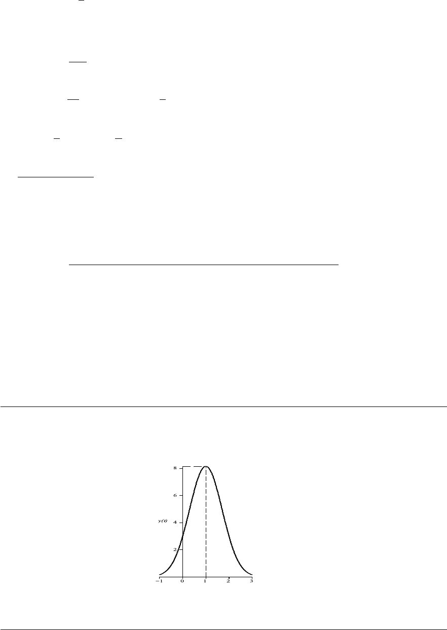
Figures
30. y = Ce
4x
− x −
1
4
32. y
2
= x
2
ln(x
2
) + 16x
2
34. y = x
2
sin x +
2x
2
π
2
36. sin(2x + y) −
x
3
3
+ e
y
= sin 2 +
2
3
38. y =
2 −
1
4
arctan
x
2
2
40. y =
8
1 − 3e
−4x
− 4x
TABLES
n
n
n x
x
x
n
n
n
y
y
y
n
n
n
n
n
n x
x
x
n
n
n
y
y
y
n
n
n
1 0.1 1.475 6 0.6 1.353368921
2 0.2 1.4500625 7 0.7 1.330518988
3 0.3 1.425311875 8 0.8 1.308391369
4 0.4 1.400869707 9 0.9 1.287062756
5 0.5 1.376852388 10 1.0 1.266596983
Table 2–A: Euler’s approximations to y
0
= x − y, y(0) = 0, on [0, 1] with h = 0.1.
FIGURES
Figure 2–A: The graph of the solution in Problem 28.
71
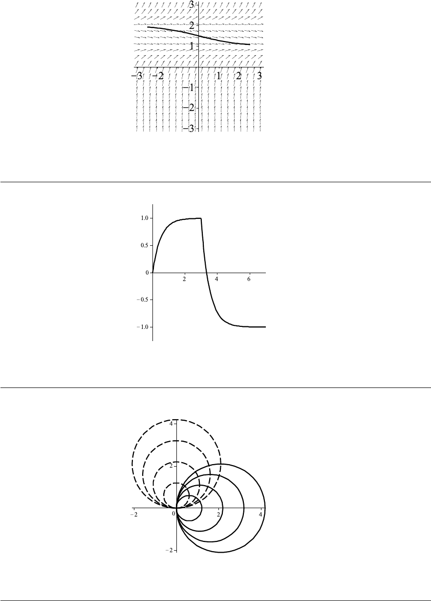
Chapter 2
Figure 2–B: The direction field and solution curve in Problem 32.
Figure 2–C: The graph of the solution in Problem 32.
Figure 2–D: Curves and their orthogonal trajectories in Problem 34.
72

CHAPTER 3: Mathematical Models and Numerical
Methods Involving First Order Equations
EXERCISES 3.2: Compartmental Analysis
2. Let x(t) denote the mass of salt in the tank at time t with t = 0 denoting the moment
when the process started. Thus we have x(0) = 0.5 kg. We use the mathematical model
described by equation (1) of the text to find x(t). Since the solution is entering the tank
with rate 6 L/min and contains 0.05 kg/L of salt,
input rate = 6 (L/min) · 0.05 (kg/L) = 0.3 (kg/min).
We can determine the concentration of salt in the tank by dividing x(t) by the volume
of the solution, which remains constant, 50 L, because the flow rate in is the same as
the flow rate out. Therefore, the concentration of salt at time t is x(t)/50 kg/L and
output rate =
x(t)
50
(kg/L) · 6 (L/min) =
3x(t)
25
(kg/min).
Then the equation (1) yields
dx
dt
= 0.3 −
3x
25
⇒
dx
dt
+
3x
25
= 0.3 , x(0) = 0.5 .
This equation is linear, has integrating factor µ(t) = exp
R
(3/25)dt
= e
3t/25
, and so
d
e
3t/25
x
dt
= 0.3e
3t/25
⇒ e
3t/25
x = 0.3
25
3
e
3t/25
+ C = 2.5e
3t/25
+ C ⇒ x = 2.5 + Ce
−3t/25
.
Using the initial condition, we find C.
0.5 = x(0) = 2.5 + C ⇒ C = −2 ,
and so the mass of salt in the tank after t minutes is
x(t) = 2.5 −2e
−3t/25
.
73

Chapter 3
If the concentration of salt in the tank is 0.03 kg/L, then the mass of salt there is
0.03 × 50 = 1.5 kg, and we solve
2.5 − 2e
−3t/25
= 1.5 ⇒ e
−3t/25
=
1
2
⇒ t =
25 ln 2
3
≈ 5.8 (min).
4. Let x(t) denote the mass of salt in the tank at time t. Since at time t = 0 the tank
contained pure water, the initial condition is x(0) = 0. We use the mathematical model
described by equation (1) of the text to find x(t). Since the solution is entering the tank
with rate 4 L/min and contains 0.2 kg/L of salt,
input rate = 4 (L/min) · 0.2 (kg/L) = 0.8 (kg/min).
We can determine the concentration of salt in the tank by dividing x(t) by the volume
v(t) of the solution at time t. Since 4 L enter the tank every minute but only 3 L flow
out, the volume of the solution after t minutes is
v(t) = v(0) + (4 −3)t = 100 + t (L).
Therefore, the concentration of salt at time t is x(t)/v(t) = x(t)/(100 + t) kg/L and
output rate =
x(t)
100 + t
(kg/L) · 3 (L/min) =
3x(t)
100 + t
(kg/min).
Then the equation (1) yields
dx
dt
= 0.8 −
3x
100 + t
⇒
dx
dt
+
3x
100 + t
= 0.8 , x(0) = 0 .
This equation is linear, has integrating factor
µ(t) = exp
Z
3dt
100 + t
= (100 + t)
3
,
and so
d ((100 + t)
3
x)
dt
= 0.8(100 + t)
3
⇒ (100 + t)
3
x = 0.2(100 + t)
4
+ C ⇒ x = 0.2(100 + t) + C(100 + t)
−3
.
Using the initial condition, we find C.
0 = x(0) = 20 + C · 10
−6
⇒ C = −2 · 10
7
,
74

Exercises 3.2
and so the mass of salt in the tank after t minutes is
x = 0.2(100 + t) −2 ·10
7
(100 + t)
−3
.
To answer the second question, we solve
x(t)
v(t
= 0.2 − 2 · 10
7
(100 + t)
−4
= 0.1 ⇒ (100 + t)
4
= 2 · 10
8
⇒ t =
4
√
2 · 10
8
− 100 = 100
4
√
2 − 1
≈ 19 (min).
6. The volume V of the room is
V = 12 × 8 × 8 = 768 ft
3
.
Let v(t) denote the amount of carbon monoxide in the room at time t. Since, at t = 0,
the room contained 3% of carbon monoxide, we have an initial condition
v(0) = 768 · 0.03 = 23.04 .
The input rate in this problem is zero, because incoming air does not contain carbon
monoxide. Next, the output rate can b e found as the concentration at time t multiplied
by the rate of outgoing flow, which is 100 ft
3
/min. Thus,
output rate =
v(t)
V
· 100 =
100v(t)
768
=
25v(t)
192
,
and the equation (1) of the text yields
dv
dt
= −
25v
192
, v(0) = 23.04 .
This is the exponential model (10), and so we can use formula (11) for the solution to
this initial value problem.
v(t) = 23.04e
−(25/192)t
.
The air in the room will be 0.01% carbon monoxide when
v(t)
V
= 10
−4
⇒
23.04e
−(25/192)t
768
= 10
−4
⇒ t =
192 ln 300
25
≈ 43.8 (min).
8. Let s(t), t ≥ 0, denote the amount of salt in the tank at time t. Thus we have s(0) = s
0
lb.
We again use the mathematical model
rate of change = input rate − output rate (3.1)
75

Chapter 3
to find s(t). Here
input rate = 4 (gal/min) · 0.5 (lb/gal) = 2 (lb/min).
Since the flow rate in is the same as the flow rate out, the volume of the solution remains
constant (200 gal), we have
c(t) =
s(t)
200
(lb/gal)
and so
output rate = 4 (gal/min) ·
s(t)
200
(lb/gal) =
s(t)
50
(lb/min).
Then (3.1) yields
ds
dt
= 2 −
s
50
⇒
ds
dt
+
s
50
= 2 .
This equation is linear, has integrating factor µ(t) = exp
R
(1/50)dt
= e
t/50
. Integrat-
ing, we get
d
e
t/50
s
dt
= 2e
t/50
⇒ s = 100 + Ce
−t/50
⇒ c(t) =
1
2
+ (C/200)e
−t/50
,
where the constant C depends on s
0
. (We do not need an explicit formula.) Taking the
limit yields
lim
t→∞
c(t) = lim
t→∞
1
2
+ (C/200)e
−t/50
=
1
2
.
10. In this problem, the dependent variable is x, the independent variable is t, and the
function f(t, x) = a − bx. Since f(t, x) = f(x), i.e., does not depend on t, the equation
is autonomous. To find equilibrium solutions, we solve
f(x) = 0 ⇒ a − bx = 0 ⇒ x =
a
b
.
Thus, x(t) ≡ a/b is an equilibrium solution. For x < a/b, x
0
= f(x) > 0 meaning that x
increases, while x
0
= f(x) < 0 when x > a/b and so x decreases. Therefore, the phase
line for the given equation is as it is shown in Fig. 3–A on page 100. From this picture,
we conclude that the equilibrium x = a/b is a sink. Thus, regardless of an initial point
x
0
, the solution to the corresponding initial value problem will approach x = a/b, as
t → ∞.
12. Equating expressions (21) evaluated at times t
a
and t
b
= 2t
a
yields
p
a
p
1
e
−Ap
1
t
a
p
1
− p
a
(1 − e
−Ap
1
t
a
)
=
p
b
p
1
e
−2Ap
1
t
a
p
1
− p
b
(1 − e
−2Ap
1
t
a
)
.
76

Exercises 3.2
With χ = e
−Ap
1
t
a
, this equation becomes
p
a
p
1
χ
p
1
− p
a
(1 − χ)
=
p
b
p
1
χ
2
p
1
− p
b
(1 − χ
2
)
⇒ p
a
p
1
(p
1
− p
b
)χ + p
a
p
b
p
1
χ
3
= p
b
p
1
(p
1
− p
a
)χ
2
+ p
a
p
b
p
1
χ
3
⇒ p
1
χ [p
a
(p
1
− p
b
) − p
b
(p
1
− p
a
)χ] = 0 ⇒ χ =
p
a
(p
1
− p
b
)
p
b
(p
1
− p
a
)
.
Hence, with t = t
a
, expression (21) yields
p
0
=
p
a
p
1
[p
a
(p
1
− p
b
)] / [p
b
(p
1
− p
a
)]
p
1
− p
a
+ p
a
[p
a
(p
1
− p
b
)] / [p
b
(p
1
− p
a
)]
⇒ p
0
=
p
2
a
p
1
(p
1
− p
b
)
p
b
(p
1
− p
a
)
2
+ p
2
a
(p
1
− p
b
)
=
p
2
a
(p
1
− p
b
)
p
b
p
1
− 2p
a
p
b
+ p
2
a
⇒ p
1
p
0
p
b
− p
2
a
= p
a
(2p
0
p
b
− p
0
p
a
− p
a
p
b
)
⇒ p
1
=
p
a
(p
a
p
b
− 2p
0
p
b
+ p
0
p
a
)
p
2
a
− p
0
p
b
,
and the formula for p
1
is proved.
For the second formula, using the expression for χ, we conclude that
χ = e
−Ap
1
t
a
=
p
a
(p
1
− p
b
)
p
b
(p
1
− p
a
)
⇒ A =
1
p
1
t
a
ln
1
χ
=
1
p
1
t
a
ln
p
b
(p
1
− p
a
)
p
a
(p
1
− p
b
)
.
Since
p
1
− p
a
= p
a
p
a
p
b
− 2p
0
p
b
+ p
0
p
a
p
2
a
− p
0
p
b
− 1
= p
a
p
a
p
b
− p
0
p
b
+ p
0
p
a
− p
2
a
p
2
a
− p
0
p
b
=
p
a
(p
b
− p
a
)(p
a
− p
0
)
p
2
a
− p
0
p
b
p
1
− p
b
=
p
a
(p
a
p
b
− 2p
0
p
b
+ p
0
p
a
)
p
2
a
− p
0
p
b
− p
b
=
p
0
p
2
a
− 2p
0
p
a
p
b
+ p
0
p
2
b
p
2
a
− p
0
p
b
=
p
0
(p
b
− p
a
)
2
p
2
a
− p
0
p
b
,
we have
p
b
(p
1
− p
a
)
p
a
(p
1
− p
b
)
=
p
b
p
a
·
p
a
(p
a
− p
0
)
p
0
(p
b
− p
a
)
=
p
b
(p
a
− p
0
)
p
0
(p
b
− p
a
)
,
and the formula for A is proved.
14. Counting time from the year 1970, we have an initial condition p(0) = 300 for the
population of alligators. Thus, the formula (11) yields
p(t) = 300e
kt
.
77

Chapter 3
In the year 1980, t = 10 and, therefore,
p(10) = 300e
k(10)
= 1500 ⇒ k =
ln 5
10
⇒ p(t) = 300e
(t ln 5)/10
.
In the year 2010, t = 2010 − 1970 = 40, and the estimated population of alligators,
according to the Malthusian law, is
p(40) = 300e
(40 ln 5)/10
= 300 · 5
4
= 187500.
16. By definition,
p
0
(t) = lim
h→0
p(t + h) − p(t)
h
.
Replacing h by −h in the above equation, we obtain
p
0
(t) = lim
h→0
p(t − h) − p(t)
−h
= lim
h→0
p(t) − p(t − h)
h
.
Adding the previous two equations together yields
2p
0
(t) = lim
h→0
p(t + h) − p(t)
h
+
p(t) − p(t − h)
h
= lim
h→0
p(t + h) − p(t − h)
h
.
Thus
p
0
(t) = lim
h→0
p(t + h) − p(t − h)
2h
.
18. Setting t = 0 for the year 2000, we obtain
t
a
= 1920 − 1900 = 20 , t
b
= 1940 − 1900 = 40 .
Thus, t
b
= 2t
a
, and so we can use formulas given in Problem 12 to find p
1
and A. With
p
0
= 76.21 , p
a
= 106.02 , p
b
= 132.16 ,
these formulas give
p
1
=
p
a
p
b
− 2p
0
p
b
+ p
0
p
a
p
2
a
− p
0
p
b
p
a
≈ 176.73 ,
A =
1
p
1
t
a
ln
p
b
(p
a
− p
0
)
p
0
(p
b
− p
a
)
≈ 0.0001929 .
We can now use the logistic equation (15).
In 1990, t = 90 and computations give p(90) ≈ 166.52.
In 2000, t = 100 and p(100) ≈ 169.35 .
The census data presented in Table 3.1 are 248.71 and 281.42, respectively.
78

Exercises 3.2
20. Assuming that only dust clouds affect the intensity of the light, we conclude that the
intensity of the light halved after passing the dust cloud.
Let s denote the distance (in light-years), and let I(s) be the intensity of the light after
passing s light-years in the dust cloud. Using the given conditions, we then obtain an
initial value problem
dI
ds
= −0.1I, I(0) = I
0
.
Using the formula (11), we find that
I(s) = I
0
e
−0.1s
.
If the thickness of the dust cloud is s
∗
, then
I(s
∗
) = I
0
e
−0.1s
∗
= (1/2)I
0
⇒ s
∗
= 10 ln 2 ≈ 6.93 .
Thus, the thickness of the dust cloud is approximately 6.93 light-years.
22. Let D(t) and S(t) denote the diameter and the surface area of the s nowball at time t,
respectively. From geometry, we know that S = πD
2
. Since we are given that D
0
(t) is
proportional to S(t), the equation describing the melting process is
dD
dt
= kS ⇒
dD
dt
= k
πD
2
⇒
dD
D
2
= kπ dt
⇒ −D
−1
= kπt + C ⇒ D = −
1
kπt + C
.
Initially, D(0) = 4, and we also know that D(30) = 3. This yields a system
4 = D(0) = −
1
C
⇒ C = −
1
4
;
3 = D(30) = −
1
30kπ + C
⇒ 30kπ + C = −
1
3
⇒ kπ = −
1
360
.
Thus,
D(t) = −
1
(−1/360)t − (1/4)
=
360
t + 90
.
The diameter D(t) of the snowball will be 2 inches when
360
t + 90
= 2 ⇒ t = 90 (min),
and, mathematically speaking, the snowball will melt infinitely long, but will never
disappear, because D(t) is a strictly decreasing approaching zero, as t → ∞.
79
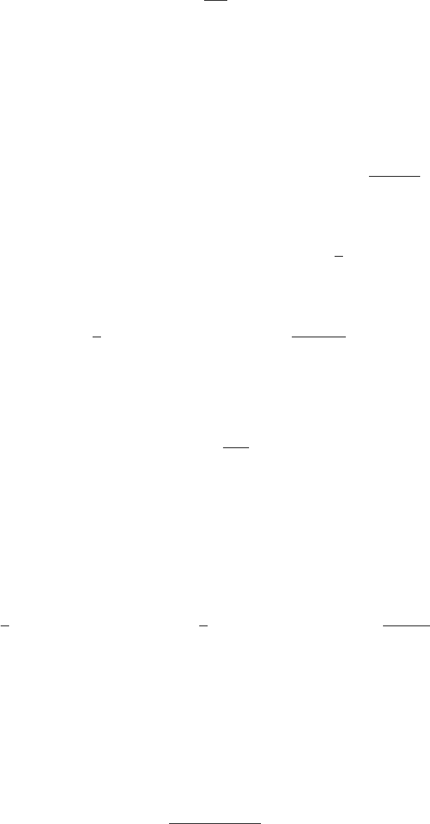
Chapter 3
24. If m(t) (with t measured in years) denotes the mass of the radioactive substance, the
law of decay says that
dm
dt
= km(t) ,
with the decay constant k depending on the substance. If the initial mass of the substance
is m(0) = m
0
, then the formula (11) of the text yields
m(t) = m
0
e
kt
.
In this problem, m
0
= 300 g, and we know that m(5) = 200 g. These data yield
200 = m(5) = 300 · e
k(5)
⇒ k =
ln(2/3)
5
,
and so the decay is governed by the equation
m(t) = 300e
[t ln(2/3)]/5
= 300
2
3
t/5
.
If only 10 g of the substance remain, them
300
2
3
t/5
= 10 ⇒ t =
5 ln(30)
ln(3/2)
≈ 41.94 (yrs).
26. (a) Let M(t) denote the mass of carbon-14 present in the burnt wood of the campfire.
Since carbon-14 decays at a rate proportional to its mass, we have
dM
dt
= −αM,
where α is the proportionality constant. This equation is linear and separable.
Using the initial condition, M(0) = M
0
, from (11) we obtain
M(t) = M
0
e
−αt
.
Given the half-life of carbon-14 to be 5550 years, we find α from
1
2
M
0
= M
0
e
−α(5550)
⇒
1
2
= e
−α(5550)
⇒ α =
ln(0.5)
−5550
≈ 0.00012489 .
Thus,
M(t) = M
0
e
−0.00012489t
.
Now we are told that after t years 2% of the original amount of carbon-14 remains
in the campfire and we are asked to determine t. Thus
0.02M
0
= M
0
e
−0.00012489t
⇒ 0.02 = e
−0.00012489t
⇒ t =
ln 0.02
−0.00012489
≈ 31323.75 (years).
80

Exercises 3.3
(b) We repeat the arguments from part (a), but use the half-life 5600 years given in
Problem 21 instead of 5550 years, to find that
1
2
M
0
= M
0
e
−α(5600)
⇒
1
2
= e
−α(5600)
⇒ α =
ln(0.5)
−5600
≈ 0.00012378 ,
and so the decay is governed by
M(t) = M
0
e
−0.00012378t
.
Therefore, 3% of the original amount of carbon-14 remains in the campfire when t
satisfies
0.03M
0
= M
0
e
−0.00012378t
⇒ 0.03 = e
−0.00012378t
⇒ t =
ln 0.03
−0.00012378
≈ 28328.95 (years).
(c) Comparing the results obtained in parts (a) and (b) with the answer to Problem 21,
that is, 31606 years, we conclude that the model is more sensitive to the percent of
the mass remaining.
EXERCISES 3.3: Heating and Cooling of Buildings
2. Let T (t) denote the temperature of the beer at time t (in minutes). According to the
Newton’s law of cooling (see (1)),
dT
dt
= K[70 − T (t)],
where we have taken H(t) ≡ U(t) ≡ 0 and M(t) ≡ 70
◦
F, with the initial condition
T (0) = 35
◦
C. Solving this initial value problem yields
dT
T − 70
= −K dt ⇒ ln |T − 70| = −Kt + C
1
⇒ T (t) = 70 − Ce
−Kt
;
35 = T (0) = 70 −Ce
−K(0)
⇒ C = 35 ⇒ T (t) = 70 − 35e
−Kt
.
To find K, we use the fact that after 3 min the temperature of the beer was 40
◦
F. Thus,
40 = T (3) = 70 −35e
−K(3)
⇒ K =
ln(7/6)
3
,
and so
T (t) = 70 − 35e
−ln(7/6)t/3
= 70 − 35
6
7
t/3
.
81

Chapter 3
Finally, after 20 min, the temperature of the beer will be
T (20) = 70 − 35
6
7
20/3
≈ 57.5 (F
◦
).
4. Let T (t) denote the temperature of the wine at time t (in minutes). According to the
Newton’s law of cooling,
dT
dt
= K[23 − T (t)],
where we have taken the outside (room’s) temperature M(t) ≡ 23
◦
C, with the initial
condition T (0) = 10
◦
C. Solving this initial value problem yields
dT
T − 23
= −K dt ⇒ ln |T − 23| = −Kt + C
1
⇒ T (t) = 23 − Ce
−Kt
;
10 = T (0) = 23 −Ce
−K(0)
⇒ C = 13 ⇒ T (t) = 23 − 13e
−Kt
.
To find K, we use the fact that after 10 min the temperature of the wine was 15
◦
C.
Thus,
15 = T (10) = 23 −13e
−K(10)
⇒ K =
ln(13/8)
10
,
and so
T (t) = 23 − 13e
−ln(13/8)t/10
= 23 − 13
8
13
t/10
.
We now solve the equation T (t) = 18.
18 = 23 −13
8
13
t/10
⇒
8
13
t/10
=
5
13
⇒ t =
10 ln(5/13)
ln(8/13)
≈ 19.7 (min).
6. The temperature function T (t) changes according to Newton’s law of cooling. Similarly
to Example 1, we conclude that, with H(t) = U(t) ≡ 0 and the outside temperature
M(t) ≡ 12
◦
C, a general solution formula (4) yields
T (t) = 12 + Ce
−Kt
.
To find C, we use the initial condition,
T (0) = T (at noon) = 21
◦
C ,
and get
21 = T (0) = 12 + Ce
−K(0)
⇒ C = 21 − 12 = 9 ⇒ T (t) = 12 + 9e
−Kt
.
82
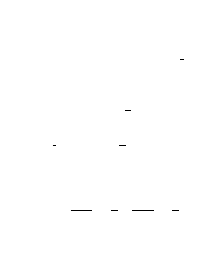
Exercises 3.3
The time constant for the building is 1/K = 3 hr; so K = 1/3 and T (t) = 12 + 9e
−t/3
.
We now solve the equation
T (t) = 12 + 9e
−t/3
= 16
to find the time when the temperature inside the building reaches 16
◦
C.
12 + 9e
−t/3
= 16 ⇒ t = 3 ln
9
4
≈ 2.43 (hr).
Thus, the temperature inside the building will be 16
◦
C at 2.43 hours after noon, that is,
approximately at 2:26 p.m.
Similarly, with the time constant 1/K = 2, we get
T (t) = 12 + 9e
−t/2
⇒ 12 + 9e
−t/2
= 16 ⇒ t = 2 ln
9
4
≈ 1.62 (hr)
or 12:37 p.m.
8. Setting t = 0 at 2:00 a.m., for the outside temperature M(t) we have
M(t) = 65 − 15 cos
πt
12
so that a general solution (4) (with K = 1/2, H(t) ≡ U(t) ≡ 0) becomes
T (t) = e
−t/2
1
2
Z
e
t/2
65 − 15 cos
πt
12
dt + C
= 65 −
540
36 + π
2
cos
πt
12
−
90π
36 + π
2
sin
πt
12
+ Ce
−t/2
.
Neglecting the exponential term, which will become insignificant with time (say, next
day), we obtain
T (t) ≈
e
T (t) = 65 −
540
36 + π
2
cos
πt
12
−
90π
36 + π
2
sin
πt
12
.
Solving
e
T
0
(t) = 0 on [0, 24) gives
540
36 + π
2
sin
πt
12
−
90π
36 + π
2
cos
πt
12
= 0 ⇒ tan
πt
12
=
π
6
⇒ t
min
=
12
π
arctan
π
6
≈ 1.84 (h) , t
max
= t
min
+ 12 ≈ 13.84 (h) .
Therefore, the lowest temperature of T (t
min
) ≈ 51.7
◦
F will be reached 1.84 (h) after
2:00 a.m., that is, at approximately 3:50 a. m.
The highest temperature of T (t
max
) ≈ 78.3
◦
F will be 12 hours later, i.e., at 3: 50 p.m.
83

Chapter 3
10. In this problem, we use the equation (9) from the text with the following values of
parameters.
K = 0.5 ,
M(t) ≡ 40 (
◦
F) ,
H(t) ≡ 0 ,
K
U
= K
1
− K = 2 − 0.5 = 1.5 ,
T
D
= 70 (
◦
F) .
Thus, we have
dT
dt
= 0.5 (40 − T ) + 1.5 (70 −T ) = 125 −2T .
Solving this linear equation yields
T (t) = e
−2t
Z
(125)e
2t
dt + C
= 62.5 + Ce
−2t
.
Setting t = 0 at 7 : 00 a.m., we find that
T (0) = 62.5 + C = 40 ⇒ C = −22.5 ⇒ T (t) = 62.5 − 22.5e
−2t
.
At 8: 00 a.m., t = 1 s o that
T (1) = 62.5 − 22.5e
−2
≈ 59.5 (
◦
F) .
Since T (t) is an increasing function with
lim
t→∞
T (t) = 62.5 ,
the temperature in the lecture hall will never reach 65
◦
F.
12. We let T
1
(t) and T
2
(t) denote the temperature of the coffee of the impatient friend and
the relaxed friend, respectively, with t = 0 meaning the time when the coffee was served.
Both functions satisfy the Newton’s law (1) of cooling with H(t) ≡ U(t) ≡ 0 and the air
temperature M(t) ≡ M
0
= const. Therefore, by (4), we have
T
k
(t) = M
0
+ C
k
e
−Kt
, k = 1, 2 . (3.2)
The constants C
k
depend on the initial temperatures of the coffee. Let’s assume that
the temperature of the coffee when served was T
0
, the amount of the coffee ordered was
84

Exercises 3.3
V
0
, the temperature of the cream was T
c
, and the teaspoon used had the capacity of
V
c
. With this assumptions, we have the initial conditions
T
2
(0) = T
0
, T
1
(0) =
T
0
V
0
+ T
c
V
c
V
0
+ V
c
(since the impatient friend immediately added a teaspoon of cream). Substituting these
initial conditions into (3.2) yields
C
1
=
T
0
V
0
+ T
c
V
c
V
0
+ V
c
− M
0
, C
2
= T
0
− M
0
.
Hence,
T
1
(t) = M
0
+
T
0
V
0
+ T
c
V
c
V
0
+ V
c
− M
0
e
−Kt
= M
0
+
(T
0
V
0
+ T
c
V
c
) − M
0
(V
0
+ V
c
)
V
0
+ V
c
e
−Kt
,
T
2
(t) = M
0
+ (T
0
− M
0
) e
−Kt
,
and so, after 5 min, the temp eratures were
T
1
(5) = M
0
+
(T
0
V
0
+ T
c
V
c
) − M
0
(V
0
+ V
c
)
V
0
+ V
c
e
−5K
,
T
2
(5) = M
0
+ (T
0
− M
0
) e
−5K
.
At this same instant of time, the second (relaxed) friend had added a teaspoon of cream
reducing his coffee’s temperature to
e
T
2
(5) =
T
2
(5)V
0
+ T
c
V
c
V
0
+ V
c
=
M
0
+ (T
0
− M
0
) e
−5K
V
0
+ T
c
V
c
V
0
+ V
c
.
We now compare T
1
(5) and
e
T
2
(5).
T
1
(5) −
e
T
2
(5) = (V
0
+ V
c
)
−1
V
c
(M
0
− T
c
)
1 − e
−5K
> 0 ,
because we assume that the cream is cooler than the air, i.e., T
c
< M
0
. Thus, the
impatient friend had the hotter coffee.
14. Since the time constant is now 72, we have K = 1/72. The temperature in the new tank
increases at the rate of 1
◦
F for every 1000 Btu. Furthermore, every hour of sunlight
provides an input of 2000 Btu to the tank. Thus,
H(t) = 1 × 2 = 2 (
◦
F/h) .
85
Chapter 3
We are given that T(0) = 110, and that the temperature M(t) outside the tank is
constantly 80
◦
F. Hence, the temperature in the tank is governed by
dT
dt
=
1
72
[80 − T (t)] + 2 = −
1
72
T (t) +
28
9
, T (0) = 110 .
Solving this separable equation gives
T (t) = 224 − Ce
−t/72
.
To find C, we use the initial condition and find that
T (0) = 110 = 224 −C ⇒ C = 114 .
This yields
T (t) = 224 − 114e
−t/72
.
So, after 12 hours of sunlight, the temperature will be
T (12) = 224 − 114e
−12/72
≈ 127.5 (
◦
F) .
16. Let A :=
p
C
2
1
+ C
2
2
. Then
C
1
cos ωt + C
2
sin ωt = A
C
1
p
C
2
1
+ C
2
2
cos ωt +
C
2
p
C
2
1
+ C
2
2
sin ωt
!
= A (α
1
cos ωt + α
2
sin ωt) . (3.3)
We note that
α
2
1
+ α
2
2
=
C
1
p
C
2
1
+ C
2
2
!
2
+
C
2
p
C
2
1
+ C
2
2
!
2
= 1 .
Therefore, α
1
and α
2
are the values of the cosine and sine functions of an angle φ, namely,
the angle satisfying
cos φ = α
1
, sin φ = α
2
⇒ tan φ =
α
2
α
1
=
C
2
C
1
. (3.4)
Hence, (3.3) becomes
C
1
cos ωt + C
2
sin ωt = A (cos φ cos ωt + sin φ sin ωt) = A cos (ωt −φ) . (3.5)
In the equation (7) of the text,
F (t) =
cos ωt + (ω/K) sin ωt
1 + (ω/K)
2
= C
1
cos ωt + C
2
sin ωt
86
Exercises 3.4
with
C
1
=
1
1 + (ω/K)
2
, C
2
=
(ω/K)
1 + (ω/K)
2
⇒ A =
s
1
1 + (ω/K)
2
2
+
(ω/K)
1 + (ω/K)
2
2
=
1 + (ω/K)
2
−1/2
.
Thus, (3.4) and (3.5) give us
F (t) =
1 + (ω/K)
2
−1/2
cos (ωt −φ) , where tan φ =
ω
K
.
EXERCISES 3.4: Newtonian Mechanics
2. This problem is a particular case of Example 1 of the text. Therefore, we can use the
general formula (6) with
m =
400
g
=
400
32
= 12.5 (slugs),
b = 10, and v
0
= v(0) = 0. But let us follow the general idea of Section 3.4, find an
equation of the motion, and solve it.
With given data, the force due to gravity is F
1
= mg = 400 lb and the air resistance
force is F
2
= −10v lb. Therefore, the velocity v(t) satisfies
12.5
dv
dt
= F
1
+ F
2
= 400 − 10v ⇒
dv
dt
= 32 − 0.8v, v(0) = 0.
Separating variables and integrating yields
dv
0.8v − 32
= −dt ⇒ ln |0.8v − 32| = −0.8t + C
1
⇒ 0.8v − 32 = ±e
C
1
e
−0.8t
= C
2
e
−0.8t
⇒ v(t) = 40 + Ce
−0.8t
.
Substituting the initial condition, v(0) = 0, we get C = −40, and so
v(t) = 40
1 − e
−0.8t
.
Integrating this equation yields
x(t) =
Z
v(t) dt = 40
Z
1 − e
−0.8t
dt = 40t + 50e
−0.8t
+ C,
and we find that C = −50 by using the initial condition, x(0) = 0. Therefore,
x(t) = 40t + 50e
−0.8t
− 50 (ft).
87

Chapter 3
When the object hits the ground, x(t) = 500 ft. Thus we solve
x(t) = 40t + 50e
−0.8t
− 50 = 500.
Since x(13) < 500 and x(14) > 500 a (positive) solution t ∈ [13, 14]. On this interval,
e
−0.8t
is very small, so we simply ignore it and solve
40t − 50 = 500 ⇒ t = 13.75 (sec).
4. Using the equation of the motion of the object found in Problem 2, we solve the equation
40t + 50e
−0.8t
− 50 = 30 ⇒ 40t + 50e
−0.8t
− 80 = 0.
This time, the solution belongs to [1, 2] and, therefore, we cannot ignore the exponential
term. Thus, we use Newton’s method (see Appendix A in the text) to approximate the
solution. We apply the recursive formula
t
n+1
= t
n
−
g(t
n
)
g
0
(t
n
)
with
g(t) = 40t + 50e
−0.8t
− 80 ⇒ g
0
(t) = 40
1 − e
−0.8t
and an initial guess t
1
= 1. Computations yield
t
1
= 1, g(t
1
) ≈ −17.53355;
t
2
= 1.79601, g(t
2
) ≈ 3.72461;
t
3
= 1.67386, g(t
3
) ≈ 0.05864;
t
4
= 1.67187, g(t
4
) ≈ 0.000017 .
Therefore, the object will hit the ground approximately after 1.67 sec.
6. We can use the model discussed in Example 1 of the text with m = 8, b = 16, g = 9.81,
and the initial velocity v
0
= −20 (the negative sign is due to the upward direction). The
formula (6) yields
x(t) =
mg
b
t +
m
b
v
0
−
mg
b
1 − e
−bt/m
=
(8)(9.81)
16
t −
8
16
20 +
(8)(9.81)
16
1 − e
−(16)t/8
= 4.905t − 12.4525
1 − e
−2t
.
88

Exercises 3.4
Because the object is released 100 m above the ground, we determine when the obj ect
strikes the ground by setting x(t) = 100 and solving for t. Since the (positive) root
belongs to [20, 24] (because x(20) < 100 and x(24) > 100), we can omit the exponential
term in x(t) and solve
4.905t − 12.4525 = 100 ⇒ t =
112.4525
4.905
≈ 22.9 (sec).
8. Since the air resistance force has different coefficients of proportionality for closed and
for opened chute, we need two differential equations describing the motion. Let x
1
(t),
x
1
(0) = 0, denote the dis tance the parachutist has fallen in t seconds with the chute
closed, and let v
1
(t) = dx
1
(t)/dt denote her velocity. With m = 100, b = b
1
= 20 N-
sec/m, and v
0
= 0 the initial value problem (4) of the text becomes
100
dv
1
dt
= 100g − 20v
1
⇒
dv
1
dt
+
1
5
v
1
= g, v
1
(0) = 0.
This is a linear equation. Solving yields
dt
e
t/5
v
1
= e
t/5
g ⇒ v
1
(t) = 5g + C
1
e
−t/5
;
0 = v
1
(0) = 5g + C
1
⇒ C
1
= −5g
⇒ v
1
(t) = 5g
1 − e
−t/5
= 49.05
1 − e
−t/5
⇒ x
1
(t) =
t
Z
0
v
1
(s)ds = 49.05
s + 5e
−s/5
s=t
s=0
= 49.05
t + 5e
−t/5
− 5
.
When the parachutist opens the chute t
1
= 30 sec after leaving the helicopter, she is
3000 − x
1
(30) ≈ 1773.14
meters above the ground and traveling at a velocity
v
1
(30) ≈ 48.93 (m/sec).
Setting the second equation, we for convenience reset the time t. Denoting by x
2
(t) the
distance passed by the parachutist during t sec from the moment when the chute opens,
and letting v
2
(t) = dx
2
(t)/dt, we have
100
dv
2
dt
= 100g − 100v
2
, v
2
(0) = v
1
(30) = 48.93, x
2
(0) = 0.
89

Chapter 3
Solving, we get
v
2
(t) = g + C
2
e
−t
;
48.93 = v
2
(0) = g + C
2
⇒ C
2
= 48.93 − g = 39.12
⇒ v
2
(t) = 9.81 + 39.12e
−t
⇒ x
2
(t) =
t
Z
0
v
2
(s)ds =
9.81s − 39.12e
−s
s=t
s=0
= 9.81t − 39.12e
−t
+ 39.12.
With the chute open, the parachutist falls 1773.14 m. Solving x
2
(t) = 1773.14 for t yields
9.81t − 39.12e
−t
+ 39.12 = 1773.14 ⇒ t
2
≈ 176.76 (sec).
Therefore, the parachutist will hit the ground t
1
+ t
2
= 30 + 176.76 = 206.76 sec after
dropping from the helicopter.
Repeating the above computations with t
1
= 60, we get
v
1
(60) ≈ 49.05 ,
x
1
(60) = 2697.75 ,
v
2
(t) = 9.81 + 39.24e
−t
,
x
2
(t) = 9.81t −39.24e
−t
+ 39.24 .
Solving x
2
(t) = 3000 − 2697.75 = 302.25 for t yields t
2
≈ 26.81 so that the parachutist
will land after t
1
+ t
2
= 86.81 (sec).
10. The motion of the object is governed by two different equations. The first equation
describes the motion in the air, the second one corresponds to the motion in the water.
For the motion in the air, we let x
1
(t) be the distance from the object to the platform
and denote by v
1
(t) = x
0
1
(t) its velocity at time t. Here we can use the model described
in Example 1 of the text with m = 2, b = b
1
= 10, v
0
= v
1
(0) = 0, and g = 9.81. Thus,
using formulas (5) and (6), we get
v(t) =
mg
b
+
v
0
−
mg
b
e
−bt/m
= 1.962
1 − e
−5t
,
x(t) =
mg
b
t −
m
b
v
0
−
mg
b
1 − e
−bt/m
= 1.962t − 0.392
1 − e
−5t
.
90

Exercises 3.4
Therefore, solving
x
1
(t) = 1.962t −0.392
1 − e
−5t
= 30,
we obtain t ≈ 15.5 sec for the time when the obje ct hit the water. The velocity of the
object at this moment was
v
1
(15.5) = 1.962
1 − e
−5(15.5)
≈ 1.962 .
We now go to the motion of the object in the water. For convenience, we reset the time.
Denoting by x
2
(t) the distance passed by the object from the water surface and by v
2
(t)
– its velocity at (reset) time t, we get we obtain initial conditions
v
2
(0) = 1.962 , x
2
(0) = 0.
For this motion, in addition to the gravity force F
g
= mg and the resistance force
F
r
= −100v, the buoyancy force F
b
= −(1/2)mg is presented. Hence, the Newton’s
second law yields
m
dv
2
dt
= mg − 100v −
1
2
mg =
1
2
mg − 100v
⇒
dv
2
dt
=
g
2
−
100
m
v
2
= 4.905 − 50v
2
.
Solving the first equation and using the initial condition yields
v
2
(t) = 0.098 + Ce
−50t
,
v
2
(0) = 0.098 + C = 1.962 ⇒ C = 1.864
⇒ v
2
(t) = 0.098 + 1.864e
−50t
⇒ x
2
(t) =
Z
t
0
v
2
(s)ds = 0.098t −0.037e
−50t
+ 0.037 .
Combining the obtained formulas for the motion of the object in the air and in the water
and taking into account the time shift made, we obtain the following formula for the
distance from the object to the platform
x(t) =
(
1.962t − 0.392 (1 − e
−5t
) , t ≤ 15.5
0.0981(t − 15.5) − 0.037e
−50(t−15.5)
+ 30.037, t > 15.5 .
1 min after the object was released, it traveled in the water for 60 − 15.5 = 44.5 sec.
Therefore, it had the velocity
v
2
(44.5) ≈ 0.098 (m/sec).
91

Chapter 3
12. We denote by x(t) the distance from the shell to the ground at time t, and let v(t) = x
0
(t)
be its velocity. Choosing positive upward direction, we get initial conditions
x(0) = 0, v(0) = 200.
There are two forces acting on the shell: the gravity force F
g
= −mg (with the negative
sign due to the upward positive direction) and the air resistance f orce F
r
= −v/20 (with
the negative sign because air resis tance acts in opposition to the motion). Thus, we
obtain an equation
m
dv
dt
= −mg −
v
20
⇒
dv
dt
= −g −
v
20m
= −g −
v
40
.
Solving this linear equation yields
v(t) = −40g + Ce
−t/40
= −392.4 + Ce
−t/40
.
Taking into account the initial condition, we find C.
200 = v(0) = −392.4 + C ⇒ C = 592.4 ⇒ v(t) = −392.4 + 592.4e
−t/40
.
At the point of maximum height, v(t) = 0. Solving
v(t) = −392.4 + 592.4e
−t/40
= 0 ⇒ t = 40 ln
592.4
392.4
≈ 16.476,
we conclude that the shell reaches its maximum height 16.476 sec after the shot. Since
x(t) =
t
Z
0
v(t) dt = −392.4t + 23696
1 − e
−t/40
,
substituting t = 16.476, we find that the maximum height of the shell is
x(16.476) ≈ 1534.81 (m).
14. We choose downward positive direction and denote by v(t) the velocity of the object
at time t. There are two forces acting on the object: the gravity force F
g
= mg and
the air resistance force F
r
= −bv
n
(with the negative sign because air resistance acts in
opposition to the motion). Thus, we obtain an equation
m
dv
dt
= mg − bv
n
⇒
dv
dt
= g −
b
m
v
n
.
Assuming that a finite limit
lim
t→∞
v(t) = V
exists and using the equation of the motion, we conclude that
92
Exercises 3.4
(i) the limit
lim
t→∞
[v(t + 1) − v(t)] = lim
t→∞
v(t + 1) − lim
t→∞
v(t) = 0;
(ii) v
0
(t) has a finite limit at infinity and, moreover,
lim
t→∞
v
0
(t) = lim
t→∞
g −
b
m
v
n
= g −
b
m
V
n
.
By Mean Value Theorem, for any N = 0, 1, 2, . . .
v(N + 1) − v(N) = v
0
(θ
N
) , θ
N
∈ (N, N + 1).
Therefore, (i) yields
lim
N→∞
v
0
(θ
N
) = 0,
and so, by (ii), v
0
(t) has zero limit at infinity and
g −
b
m
V
n
= 0 ⇒ V =
n
r
mg
b
.
16. The total torque exerted on the flywheel is the sum of the torque exerted by the motor
and the retarding torque due to friction. Thus, by Newton’s second law for rotation, we
have
I
dω
dt
= T − k
√
ω with ω(0) = ω
0
,
where I is the moment of inertia of the flywheel, ω(t) is the angular velocity, dω/dt is the
angular acceleration, T is the constant torque exerted by the motor, and k is a positive
constant of proportionality for the torque due to friction. Separating variables yields
dω
√
ω − (T/k)
= −
k
I
dt.
Since
Z
dx
√
x − a
=
x = y
2
, dx = 2y dy
= 2
Z
y dy
y − a
= 2
Z
dy + a
Z
dy
y − a
= 2 (y + a ln |y − a|) + C = 2
√
x + a ln |
√
x − a|
+ C,
integrating the above equation, we obtain
2
√
ω + (T/k) ln
√
ω − (T/k)
+ C = −
k
I
t
⇒ k
√
ω + T ln
k
√
ω − T
= −
k
2
2I
t + C
1
.
93

Chapter 3
Using the initial condition ω(0) = ω
0
, we find that
C
1
= k
√
ω
0
+ T ln |k
√
ω
0
− T |.
Hence, ω(t) is given implicitly by
k
√
ω −
√
ω
0
+ T ln
k
√
ω − T
k
√
ω
0
− T
= −
k
2
t
2I
.
18. Since we assume that there is no resistance force, there are only two forces acting on the
object: F
g
, the force due to gravity, and F
f
, the friction force. Using Fig. 3.11 in the
text, we obtain
F
g
= mg sin 30
◦
=
mg
2
,
F
f
= −µN = −µmg cos 30
◦
= −
µmg
√
3
2
,
and so the equation describing the motion is
m
dv
dt
=
mg
2
−
µmg
√
3
2
⇒
dv
dt
=
g
2
1 − µ
√
3
=
g
5 −
√
3
10
with the initial condition v(0) = 0. Therefore,
v(t) =
t
Z
0
g
5 −
√
3
10
ds =
g
5 −
√
3
10
s
s=t
s=0
=
g
5 −
√
3
10
t
⇒ x(t) =
t
Z
0
v(s)ds =
g
5 −
√
3
20
s
2
s=t
s=0
=
g
5 −
√
3
20
t
2
.
Solving
x(t) =
g
5 −
√
3
20
t
2
= 5 ⇒ t
∗
=
10
q
g
5 −
√
3
,
we conclude that the object will reach the bottom of the plane t
∗
sec after it is released
having the velocity
v (t
∗
) =
g
5 −
√
3
10
·
10
q
g
5 −
√
3
=
r
g
5 −
√
3
≈ 5.66 (m/sec).
We remark that the mass of the object is irrelevant.
94

Exercises 3.4
20. The gravitational force F
g
down the incline is
F
g
= mg sin α,
the force F
f
due to static friction satisfies
F
f
≤ µN = µmg cos α .
The object will slide if F
g
> F
f
. In the worst case, that is, in the case when the friction
force is the largest possible, the angle α must satisfy
mg sin α > µmg cos α ⇒ tan α > µ ⇒ α > arctan µ.
Thus, α
0
= arctan µ.
22. In this problem, there are two forces acting on a sailboat: a constant horizontal force
due to the wind and a force due to the water resistance that acts in opposition to the
motion of the sailboat. All of the motion occurs along a horizontal axis. On this axis,
we choose the origin to be the point, where the boat begins to “plane”, set t = 0 at this
moment, and let x(t) and v(t) = x
0
(t) denote the dis tance the sailb oat travels in time t
and its velocity, respectively. The force due to the wind is still
F
w
= 600 N.
The force due to water resistance is now
F
r
= −60v N.
Applying Newton’s second law we obtain
50
dv
dt
= 600 − 60v ⇒
dv
dt
=
6
5
(10 − v).
Since the velocity of the sailboat at t = 0 is 5 m/sec, a model for the velocity of the
moving sailboat is expressed as the initial value problem
dv
dt
=
6
5
(10 − v), v(0) = 5 .
Separating variables and integrating yields
dv
v − 10
= −
6dt
5
⇒ ln(v − 10) = −
6t
5
+ C
1
⇒ v(t) = 10 + Ce
−6t/5
.
95

Chapter 3
Setting v = 5 when t = 0, we find that 5 = 10+C so that C = −5 and v(t) = 10−5e
−6t/5
.
The limiting velocity of the sailboat under these conditions is
lim
t→∞
v(t) = lim
t→∞
10 − 5e
−6t/5
= 10 (m/sec).
To find the equation of motion, we integrate v(t) using the initial condition x(0) = 0.
x(t) =
t
Z
0
10 − 5e
−6s/5
ds =
10s +
25
6
e
−6s/5
t
0
= 10t +
25
6
e
−6t/5
− 1
.
24. Dividing the equation by m
0
− αt yields
dv
dt
= −g +
αβ
m
0
− αt
⇒ v(t) =
t
Z
0
−g +
αβ
m
0
− αs
ds + v(0)
= [−gs − β ln(m
0
− αs)]|
s=t
s=0
= −gt + β ln
m
0
m
0
− αt
,
where we used the condition 0 ≤ t < m
0
/α so that m
0
− αt > 0.
Since the height h(t) of the rocket satisfies h(0) = 0, we find
h(t) =
t
Z
0
v(s)ds =
t
Z
0
−gs + β ln
m
0
m
0
− αs
ds
=
−
gs
2
2
+ βs ln m
0
+
β
α
(m
0
− αs) ln
m
0
− αs
e
s=t
s=0
= βt −
gt
2
2
−
β
α
(m
0
− αt) ln
m
0
m
0
− αt
.
EXERCISES 3.5: Electrical Circuits
2. Capacitor voltage = −
10000
100000001
cos 100t +
100000000
100000001
sin 100t +
10000
100000001
e
−1000000t
V
Resistor voltage =
10000
100000001
cos 100t +
1
100000001
sin 100t −
10000
100000001
e
−1000000t
V
Current =
10000
100000001
cos 100t +
1
100000001
sin 100t −
10000
100000001
e
−1000000t
A
4. From (2), I =
1
L
Z
E(t)dt. From the derivative of (4), I = C
dE
dt
96

Exercises 3.7
6. Multiply (2) by I to derive
d
dt
1
2
LI
2
+ RI
2
= EI (power generated by the voltage
source equals the power inserted into the inductor plus the power dissipated by the
resistor). Multiply the equation above (4) by I, replace I by dq/dt and then replace q by
CE
C
in the capacitor term, and derive RI
2
+
d
dt
1
2
CE
2
C
= EI (power generated by
the voltage source equals the power inserted into the capacitor plus the power dissipated
by the resistor).
8. In cold weather, 96.27 hours. In (extremely) humid weather, 0.0485 seconds.
EXERCISES 3.6: Improved E uler’s Method
6. For k = 0, 1, 2, . . . , n, let x
k
= kh and z
k
= f (x
k
), where h = 1/n.
(a) h (z
0
+ z
1
+ z
2
+ ··· + z
n−1
)
(b) (h/2) (z
0
+ 2z
1
+ 2z
2
+ ··· + 2z
n−1
+ z
n
)
(c) (h/2) (z
0
+ 2z
1
+ 2z
2
+ ··· + 2z
n−1
+ z
n
)
8. See Table 3–A on page 98.
10. See Table 3–B on page 98.
12. φ(π) ≈ y (π; π2
−4
) ≈ 1.09589
14. 2.36 at x = 0.78
16. x = 1.26
20. See Table 3–C on page 99.
EXERCISES 3.7: Higher-Order Numerical Methods: Taylor and Runge-Kutta
2. y
n+1
= y
n
+ h
x
n
y
n
− y
2
n
+
h
2
/2!
y
n
+ (x
n
− 2y
n
)
x
n
y
n
− y
2
n
4. y
n+1
= y
n
+ h
x
2
n
+ y
n
+
h
2
/2!
2x
n
+ x
2
n
+ y
n
+
h
3
/3!
2 + 2x
n
+ x
2
n
+ y
n
+
h
4
/4!
2 + 2x
n
+ x
2
n
+ y
n
6. Order 2: φ(1) ≈ 0.62747
Order 4: φ(1) ≈ 0.63231
97

Chapter 3
8. 0.63211
10. 0.70139 with h = 0.25
12. −0.928 at x = 1.2
14. 1.00000 with h = π/16
16. See Table 3–D on page 100.
20. x(10) ≈ 2.23597 ×10
−4
TABLES
Table 3–A: Improved Euler’s method approximations in Problem 8.
x
n
1.2 1.4 1.6 1.8
y
n
1.48 2.24780 3.65173 6.88712
Table 3–B: Improved Euler’s method approximations in Problem 10.
x
n
x
n
x
n
y
n
y
n
y
n
0.1 1.15845
0.2 1.23777
0.3 1.26029
0.4 1.24368
0.5 1.20046
0.6 1.13920
0.7 1.06568
0.8 0.98381
0.9 0.89623
1.0 0.80476
98
Tables
Table 3–C: Improved Euler’s method approximations in Problem 20.
t
t
t r = 1.0
r = 1.0
r = 1.0 r = 1.5
r = 1.5
r = 1.5 r = 2.0
r = 2.0
r = 2.0
0 0.0 0.0 0.0
0.2 1.56960 1.41236 1.19211
0.4 2.63693 2.14989 1.53276
0.6 3.36271 2.51867 1.71926
0.8 3.85624 2.70281 1.84117
1.0 4.19185 2.79483 1.92743
1.2 4.42005 2.84084 1.99113
1.4 4.57524 2.86384 2.03940
1.6 4.68076 2.87535 2.07656
1.8 4.75252 2.88110 2.10548
2.0 4.80131 2.88398 2.12815
2.2 4.83449 2.88542 2.14599
2.4 4.85705 2.88614 2.16009
2.6 4.87240 2.88650 2.17126
2.8 4.88283 2.88668 2.18013
3.0 4.88992 2.88677 2.18717
3.2 4.89475 2.88682 2.19277
3.4 4.89803 2.88684 2.19723
3.6 4.90026 2.88685 2.20078
3.8 4.90178 2.88686 2.20360
4.0 4.90281 2.88686 2.20586
4.2 4.90351 2.88686 2.20765
4.4 4.90399 2.88686 2.20908
4.6 4.90431 2.88686 2.21022
4.8 4.90453 2.88686 2.21113
5.0 4.90468 2.88686 2.21186
99
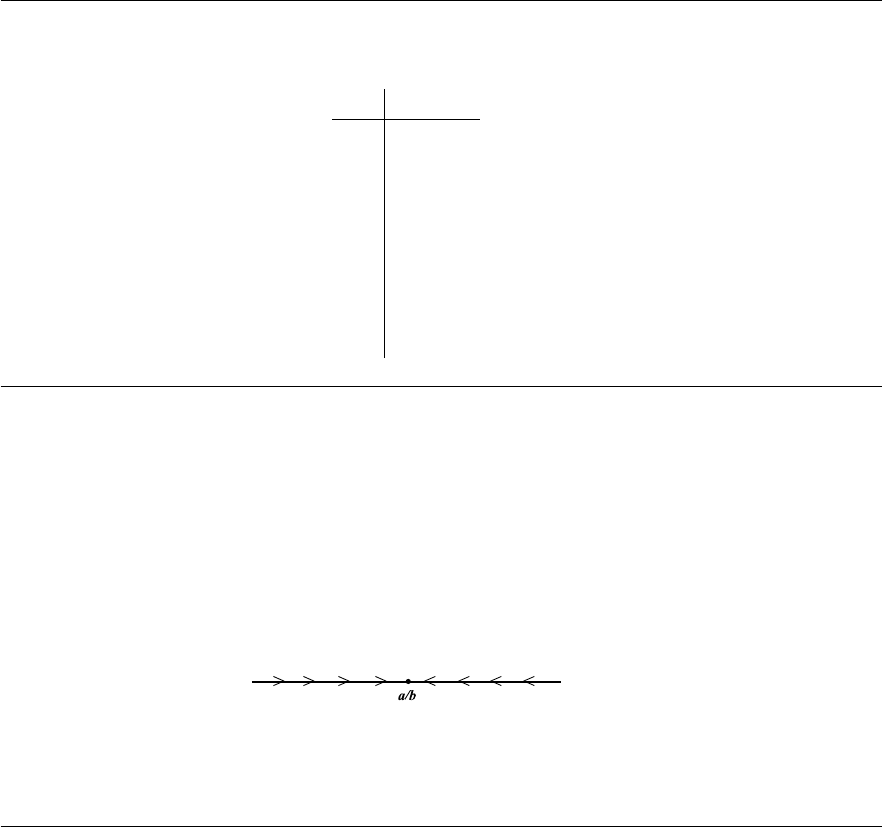
Chapter 3
Table 3–D: Fourth-order Runge-Kutta approximations in Problem 16.
x
n
x
n
x
n
y
n
y
n
y
n
0.5 1.17677
1.0 0.37628
1.5 1.35924
2.0 2.66750
2.5 2.00744
3.0 2.72286
3.5 4.11215
4.0 3.72111
FIGURES
Figure 3–A: The phase line for x
0
= a − bx in Problem 10.
100

CHAPTER 4: Linear Second Order Equations
EXERCISES 4.1: Introduction: The Mass-Spring Oscillator
2. (a) Substituting cy(t) into the equation yields
m(cy)
00
+ b(cy)
0
+ k(cy) = c (my
00
+ by
0
+ ky) = 0.
(b) Substituting y
1
(t) + y
2
(t) into the given equation, we obtain
m (y
1
+ y
2
)
00
+ b (y
1
+ y
2
)
0
+ k (y
1
+ y
2
) = (my
00
1
+ by
0
1
+ ky
1
)
+ (my
00
2
+ by
0
2
+ ky
2
) = 0.
4. With F
ext
= 0, m = 1, k = 9, and b = 6 equation (3) becomes
y
00
+ 6y
0
+ 9y = 0 .
Substitution y
1
= e
−3t
and y
2
= te
−3t
yields
e
−3t
00
+ 6
e
−3t
0
+ 9
e
−3t
= 9e
−3t
− 18e
−3t
+ 9e
−3t
= 0,
te
−3t
00
+ 6
te
−3t
0
+ 9
te
−5t
= (9t − 6)e
−3t
+ 6(1 − 3t)e
−3t
+ 9te
−3t
= 0.
Thus, y
1
= e
−3t
and y
2
= te
−3t
are solutions to the given equation.
Both solutions approach zero as t → ∞.
6. With F
ext
= 2 cos 2t, m = 1, k = 4, and b = 0, the equation (3) has the form
y
00
+ 4y
0
= 2 cos 2t .
For y(t) = (1/2)t sin 2t, one has
y
0
(t) =
1
2
sin 2t + t cos 2t, y
00
(t) = 2 cos 2t −2t sin 2t;
y
00
+ 4y
0
= (2 cos 2t − 2t sin 2t) + 4
1
2
t sin 2t
= 2 cos 2t.
101

Chapter 4
Hence, y(t) = (1/2)t sin 2t is a solution. Clearly, this function satisfies the initial condi-
tions. Indeed,
y(0) =
1
2
t sin 2t
t=0
= 0
y
0
(0) =
1
2
sin 2t + t cos 2t
t=0
= 0.
As t increases, the spring will eventually break down since the solution oscillates with
the magnitude increasing without bound.
8. For y = A cos 3t + B sin 3t,
y
0
= −3A sin 3t + 3B cos 3t, y
00
= −9A cos 3t − 9B sin 3t.
Inserting y, y
0
, and y
00
into the given equation and matching coefficients yield
y
00
+ 2y
0
+ 4y = 5 sin 3t
⇒ (−9A cos 3t − 9B sin 3t) + 2(−3A sin 3t + 3B cos 3t) + 4(A cos 3t + B sin 3t)
= (−5A + 6B) cos 3t + (−6A − 5B) sin 3t = 5 sin 3t
⇒
−5A + 6B = 0
−6A − 5B = 5
⇒
A = −30/61
B = −25/61.
Thus,
y = −(30/61) cos 3t − (25/61) sin 3t
is a synchronous solution to y
00
+ 2y
0
+ 4y = 5 sin 3t.
10. (a) We seek solutions to (7) of the form y = A cos Ωt + B sin Ωt. Since
y
0
= −AΩ sin Ωt + BΩ cos Ωt,
y
00
= −AΩ
2
cos Ωt − BΩ
2
sin Ωt,
we insert these equations into (7), collect similar terms, and match co efficients.
m(−AΩ
2
cos Ωt − BΩ
2
sin Ωt) + b(−AΩ sin Ωt + BΩ cos Ωt)
+k(A cos Ωt + B sin Ωt)
=
−mAΩ
2
+ bBΩ + kA
cos Ωt +
−mBΩ
2
− bAΩ + kB
sin Ωt = cos Ωt
⇒
(
−mAΩ
2
+ bBΩ + kA = 1
−mBΩ
2
− bAΩ + kB = 0
102

Exercises 4.2
⇒
(
A (−mΩ
2
+ k) + B (bΩ) = 1
A (−bΩ) + B (−mΩ
2
+ k) = 0
⇒ A = −
mΩ
2
− k
(mΩ
2
− k)
2
+ b
2
Ω
2
, B =
bΩ
(mΩ
2
− k)
2
+ b
2
Ω
2
⇒ y = −
mΩ
2
− k
(mΩ
2
− k)
2
+ b
2
Ω
2
cos Ωt +
bΩ
(mΩ
2
− k)
2
+ b
2
Ω
2
sin Ωt .
(b) With m = 1, b = 0.1, and k = 25, the coefficients A and B in part (a) are
A(Ω) = −
Ω
2
− 25
(Ω
2
− 25)
2
+ 0.01
, B(Ω) =
0.1Ω
2
(Ω
2
− 25)
2
+ 0.01
.
The graphs of these functions are shown in Fig. 4–A on page 173.
(c) If m = 1, b = 0, and k = 25, the coefficients A and B in part (a) become
A(Ω) = −
1
Ω
2
− 25
, B(Ω) ≡ 0 .
The graphs of these functions are shown in Fig. 4–B, page 173.
(d) If b = 0, then equation (7) reduces to my
00
+ ky = cos Ωt.
Substituting y = A cos Ωt + B sin Ωt yields
m
−AΩ
2
cos Ωt − BΩ
2
sin Ωt
+ k (A cos Ωt + B sin Ωt) = cos Ωt
⇒
−mΩ
2
+ k
(A cos Ωt + B sin Ωt) = cos Ωt .
Assuming now that Ω =
p
k/m, we get −mΩ
2
+ k = 0, and so the above equation
is impossible with any choice of A and B.
(e) Differentiating y = (2mΩ)
−1
t sin Ωt twice, we obtain
y
0
=
1
2mΩ
(sin Ωt + tΩ cos Ωt) , y
00
=
1
2m
(2 cos Ωt − tΩ sin Ωt)
my
00
+ ky =
1
2
(2 cos Ωt − tΩ sin Ωt) +
k
2mΩ
t sin Ωt
cos Ωt +
−Ω +
k
mΩ
t sin Ωt
2
= cos Ωt ,
since −Ω + k/(mΩ) = 0 if Ω =
p
k/m.
EXERCISES 4.2: Homogeneous Linear Equations: The General Solution
2. The auxiliary equation, r
2
+ 6r + 9 = (r + 3)
2
= 0, has a double root r = −3. Therefore,
e
−3t
and te
−3t
are two linearly independent solutions for this differential equation, and
103

Chapter 4
a general solution is given by
y(t) = c
1
e
−3t
+ c
2
te
−3t
,
where c
1
and c
2
are arbitrary constants.
4. The auxiliary equation for this problem is r
2
−r −2 = (r −2)(r + 1) = 0, which has the
roots r = 2 and r = −1. Thus {e
2t
, e
−t
} is a set of two linearly independent solutions to
this differential equation. Therefore, a general solution is given by
y(t) = c
1
e
2t
+ c
2
e
−t
,
where c
1
and c
2
are arbitrary constants.
6. The auxiliary equation for this problem is r
2
−5r + 6 = 0 with roots r = 2, 3. Therefore,
a general solution is
y(t) = c
1
e
2t
+ c
2
e
3t
.
8. Solving the auxiliary equation, 6r
2
+ r − 2 = 0, yields r = −2/3, 1/2. Thus a general
solution is given by
y(t) = c
1
e
t/2
+ c
2
e
−2t/3
,
where c
1
and c
2
are arbitrary constants.
10. Solving the auxiliary equation, 4r
2
− 4r + 1 = (2r − 1)
2
= 0, we conclude that r = 1/2
is its double root. Therefore, a general solution to the given differential equation is
y(t) = c
1
e
t/2
+ c
2
te
t/2
.
12. The auxiliary equation for this problem is 3r
2
+11r −7 = 0. Using the quadratic formula
yields
r =
−11 ±
√
121 + 84
6
=
−11 ±
√
205
6
.
Thus, a general solution to the given equation is
y(t) = c
1
e
(−11+
√
205)t/6
+ c
2
e
(−11−
√
205)t/6
.
14. The auxiliary equation for this problem is r
2
+ r = 0, which has roots r = −1, 0. Thus,
a general solution is given by
y(t) = c
1
e
−t
+ c
2
,
104

Exercises 4.2
where c
1
, c
2
are arbitrary constants. To satisfy the initial conditions, y(0) = 2, y
0
(0) = 1,
we find the derivative y
0
(t) = −c
1
e
−t
and solve the system
y(0) = c
1
e
−0
+ c
2
= c
1
+ c
2
= 2
y
0
(0) = −c
1
e
−0
= −c
1
= 1
⇒
c
1
= −1
c
2
= 3.
Therefore, the solution to the given initial value problem is
y(t) = −e
−t
+ 3 .
16. The auxiliary equation for this problem, r
2
− 4r + 3 = 0, has roots r = 1, 3. Therefore,
a general solution is given by
y(t) = c
1
e
t
+ c
2
e
3t
⇒ y
0
(t) = c
1
e
t
+ 3c
2
e
3t
.
Substitution of y(t) and y
0
(t) into the initial conditions yields the system
y(0) = c
1
+ c
2
= 1
y
0
(0) = c
1
+ 3c
2
= 1/3
⇒
c
1
= 4/3
c
2
= −1/3.
Thus, the solution satisfying the given initial conditions is
y(t) =
4
3
e
t
−
1
3
e
3t
.
18. The auxiliary equation for this differential equation is r
2
−6r + 9 = (r −3)
2
= 0. We see
that r = 3 is a repeated root. Thus, two linearly independent solutions are y
1
(t) = e
3t
and y
2
(t) = te
3t
. This means that a general solution is given by y(t) = c
1
e
3t
+ c
2
te
3t
.
To find the constants c
1
and c
2
, we substitute the initial conditions into the general
solution and its derivative, y
0
(t) = 3c
1
e
3t
+ c
2
(e
3t
+ 3te
3t
), and obtain
y(0) = 2 = c
1
y
0
(0) = 25/3 = 3c
1
+ c
2
.
So, c
1
= 2 and c
2
= 7/3. Therefore, the solution that satisfies the initial conditions is
given by
y(t) = 2e
3t
+
7
3
te
3t
=
7t
3
+ 2
e
3t
.
105

Chapter 4
20. The auxiliary equation for this differential equation, r
2
− 4r + 4 = (r − 2)
2
= 0, has
a double root r = 2. Thus, two linearly independent solutions are y
1
(t) = e
2t
and
y
2
(t) = te
2t
. This means that a general solution is given by y(t) = (c
1
+ c
2
t) e
2t
.
Substituting the initial conditions into the general solution and its derivative yields
y(1) = (c
1
+ c
2
t) e
2t
|
t=1
= (c
1
+ c
2
) e
2
= 1
y
0
(1) = (c
2
+ 2c
1
+ 2c
2
t) e
2t
|
t=1
= (2c
1
+ 3c
2
) e
2
= 1 .
So, c
1
= 2e
−2
and c
2
= −e
−2
. Therefore, the solution is
y(t) =
2e
−2
− e
−2
t
e
2t
= (2 − t)e
2t−2
.
22. We substitute y = e
rt
into the given equation and get
3re
rt
− 7e
rt
= (3r − 7)e
rt
= 0.
Therefore,
3r − 7 = 0 ⇒ r =
7
3
,
and a general solution to the given differential equation is y(t) = ce
7t/3
, where c is an
arbitrary constant.
24. Similarly to the previous problem, we find the characteristic equation, 3r+11 = 0, which
has the root r = −11/3. Therefore, a general solution is given by z(t) = ce
−11t/3
.
26. (a) Substituting boundary conditions into y(t) = c
1
cos t + c
2
sin t yields
2 = y(0) = c
1
0 = y (π/2) = c
2
.
Thus, c
1
and c
2
are determined uniquely, and so the given boundary value problem
has a unique solution y = 2 cos t.
(b) Similarly to part (a), we obtain a system to determine c
1
and c
2
.
2 = y(0) = c
1
0 = y (π) = −c
1
.
However, this system is inconsistent, and so there is no solution satisfying given
boundary conditions.
106
Exercises 4.2
(c) This time, we come up with a system
2 = y(0) = c
1
−2 = y (π) = −c
1
,
which has infinitely many solutions given by c
1
= 2 and c
2
– arbitrary. Thus, the
boundary value problem has infinitely many solutions of the form
y = 2 cos t + c
2
sin t .
28. Assuming that y
1
(t) = e
3t
and y
2
(t) = e
−4t
are linearly dependent on (0, 1), we conclude
that, for some constant c and all t ∈ (0, 1),
y
1
(t) = cy
2
(t) ⇒ e
3t
= ce
−4t
⇒ e
7t
= c.
Since an exponential function is strictly monotone, this is a contradiction. Hence, given
functions are linearly independent on (0, 1).
30. These functions are linearly independent, because the equality y
1
(t) ≡ cy
2
(t) would
imply that
t
2
cos(ln t) ≡ ct
2
sin(ln t) ⇒ cot(ln t) ≡ c
on (0, 1), which is false.
32. These two functions are linearly dependent since y
1
(t) ≡ 0 ·y
2
(t).
34. (a) This formula follows from the definition of 2 × 2 determinant.
(b, c) If y
1
(t) and y
2
(t) are linearly independent on I, then W [y
1
, y
2
](t) is never zero on I
since, otherwise, these functions would be linearly dependent by Lemma 1. On the
other hand, if y
1
(t) and y
2
(t) are any two differentiable functions that are linearly
dependent on I, then, say, y
1
(t) ≡ cy
2
(t) on I and so
W [y
1
, y
2
](t) = y
1
(cy
1
)
0
− y
0
1
(cy
1
) ≡ 0 on I.
36. Assume to the contrary that e
r
1
t
, e
r
2
t
, and e
r
3
t
are linearly dependent. Without loss of
generality, let
e
r
1
t
= c
1
e
r
2
t
+ c
2
e
r
3
t
⇒ e
(r
1
−r
2
)t
= c
1
+ c
2
e
(r
3
−r
2
)t
107

Chapter 4
for all t. Differentiating this identity, we obtain
(r
1
− r
2
) e
(r
1
−r
2
)t
≡ c
2
(r
3
− r
2
) e
(r
3
−r
2
)t
.
Since r
1
− r
2
6= 0, dividing both sides by (r
1
− r
2
) e
(r
1
−r
2
)t
, we obtain
c
2
(r
3
− r
2
)
(r
1
− r
2
)
e
(r
3
−r
1
)t
≡ 1 ⇒ ce
(r
3
−r
1
)t
≡ 1
on (−∞, ∞), which is a contradiction (r
3
− r
1
6= 0!).
38. The auxiliary equation for this problem is r
3
− 6r
2
− r + 6 = 0. Factoring yields
r
3
− 6r
2
− r + 6 =
r
3
− 6r
2
− (r − 6) = r
2
(r − 6) − (r − 6) = (r − 6)
r
2
− 1
.
Thus the roots of the auxiliary equation are r = ±1 and r = 6. Therefore, the functions
e
t
, e
−t
, and e
6t
are solutions to the given equation, and they are linearly independent on
(−∞, ∞) (see Problem 40), and a general solution to the equation y
000
−6y
00
−y
0
+6y = 0
is given by
y(t) = c
1
e
t
+ c
2
e
−t
+ c
3
e
6t
.
40. The auxiliary equation associated with this differential equation is r
3
−7r
2
+7r +15 = 0.
We see, by inspection, that r = −1 is a root. Dividing r
3
− 7r
2
+ 7r + 15 by r + 1, we
find that
r
3
− 7r
2
+ 7r + 15 = (r + 1)(r
2
− 8r + 15) = (r + 1)(r − 3)(r − 5).
Hence r = −1, 3, 5 are the roots to the auxiliary equation, and a general solution is
y(t) = c
1
e
−t
+ c
2
e
3t
+ c
3
e
5t
.
42. By inspection, we see that r = 1 is a root of the auxiliary equation, r
3
+ r
2
−4r + 2 = 0.
Dividing the polynomial r
3
+ r
2
− 4r + 2 by r − 1 yields
r
3
+ r
2
− 4r + 2 = (r − 1)
r
2
+ 2r − 2
.
Hence, two other roots of the auxiliary equation are r = −1±
√
3, and a general solution
is given by
y(t) = c
1
e
t
+ c
2
e
(−1+
√
3)t
+ c
3
e
(−1−
√
3)t
.
108

Exercises 4.2
44. First we find a general solution to the equation y
000
−2y
00
−y
0
+ 2y = 0. Its characteristic
equation, r
3
− 2r
2
− r + 2 = 0, has roots r = 2, 1, and −1, and so a general solution is
given by
y(t) = c
1
e
2t
+ c
2
e
t
+ c
3
e
−t
.
Differentiating y(t) twice yields
y
0
(t) = 2c
1
e
2t
+ c
2
e
t
− c
3
e
−t
, y
00
(t) = 4c
1
e
2t
+ c
2
e
t
+ c
3
e
−t
.
Now we substitute y, y
0
, and y
00
into the initial conditions and find c
1
, c
2
, and c
3
.
y(0) = c
1
+ c
2
+ c
3
= 2
y
0
(0) = 2c
1
+ c
2
− c
3
= 3
y
00
(0) = 4c
1
+ c
2
+ c
3
= 5
⇒
c
1
= 1
c
2
= 1
c
3
= 0.
Therefore, the solution to the given initial value problem is
y(t) = e
2t
+ e
t
.
46. (a) The characteristic equation associated with y
00
− y = 0 is r
2
− 1 = 0, which has
distinct real roots r = ±1. Thus, a general solution is given by
y(t) = c
1
e
t
+ c
2
e
−t
.
Differentiating y(t) yields y
0
(t) = c
1
e
t
−c
2
e
−t
. We now substitute y and y
0
into the
initial conditions for cosh t to find its explicit formula.
y(0) = c
1
+ c
2
= 1
y
0
(0) = c
1
− c
2
= 0
⇒
c
1
= 1/2
c
2
= 1/2 .
Therefore,
cosh t =
e
t
+ e
−t
2
.
Similarly, for sinh t, we have
y(0) = c
1
+ c
2
= 0
y
0
(0) = c
1
− c
2
= 1
⇒
c
1
= 1/2
c
2
= −1/2 .
Therefore,
sinh t =
e
t
− e
−t
2
.
109

Chapter 4
Applying derivative rules, we find that
d
dt
cosh t =
d
dt
e
t
+ e
−t
2
=
(e
t
+ e
−t
)
0
2
=
e
t
− e
−t
2
= sinh t ,
d
dt
sinh t =
d
dt
e
t
− e
−t
2
=
(e
t
− e
−t
)
0
2
=
e
t
+ e
−t
2
= cosh t .
(b) It easily follows from the initial conditions–cosh 0 = 1 and s inh 0 = 0– that cosh t
and sinh t are linearly independent on −∞, ∞. Indeed, since sinh t is not identically
zero, neither of them is a constant multiple of the other. By Theorem 2, a general
solution to y
00
− y = 0 is y(t) = c
1
cosh t + c
2
sinh t.
(c) Let r
1
= α + β and r
2
= α − β be to real distinct roots of the auxiliary equation
ar
2
+ br + c = 0. Then a general solution to ay
00
+ by
0
+ cy = 0 has the form
y = C
1
e
r
1
+ C
2
e
r
2
= e
α
C
1
e
βt
+ C
2
e
−βt
. (4.1)
It follows from the explicit formulas obtained in part (a) that
cosh(βt) + sinh(βt) = e
βt
, cosh(βt) −sinh(βt) = e
−βt
.
Substituting these expressions into (4.1) yields
y = e
αt
[C
1
(cosh(βt) + sinh(βt)) + C
2
(cosh(βt) −sinh(βt))]
= e
αt
[(C
1
+ C
2
) cosh(βt) + (C
1
− C
2
) sinh(βt)] = e
αt
[c
1
cosh(βt) + c
2
sinh(βt)] ,
where c
1
= C
1
+ C
2
and c
2
= C
1
− C
2
are arbitrary constants.
(d) The auxiliary equation for y
00
+ y
0
− 6y = 0, which is r
2
+ r − 6 = 0, has two real
distinct roots r = −3, 2. Solving the system
(
α + β = −3
α −β = 2 ,
we find that α = −1/2, β = −5/2. Hence, a general s olution is
y = e
−t/2
[c
1
cosh(−5t/2) + c
2
sinh(−5t/2)] = e
−t/2
[c
1
cosh(5t/2) − c
2
sinh(5t/2)]
⇒ y
0
= e
−t/2
[−(c
1
/2) cosh(5t/2) + (c
2
/2) sinh(5t/2)
+ (5c
1
/2) sinh(5t/2) − (5c
2
/2) cosh(5t/2)] .
110
Exercises 4.3
To satisfy the initial conditions, we solve the system
2 = y(0) = c
1
−17/2 = y
0
(0) = −(c
1
/2) − (5c
2
/2)
⇒
c
1
= 2
c
2
= 3 .
Therefore, the answer is
y = e
−t/2
[2 cosh(5t/2) − 3 sinh(5t/2)] .
EXERCISES 4.3: Auxiliary Equations with Complex Roots
2. The auxiliary equation in this problem is r
2
+ 1 = 0, which has roots r = ±i. We see
that α = 0 and β = 1. Thus, a general solution to the differential equation is given by
y(t) = c
1
e
(0)t
cos t + c
2
e
(0)t
sin t = c
1
cos t + c
2
sin t.
4. The auxiliary equation, r
2
− 10r + 26 = 0, has roots r = 5 ± i. So, α = 5, β = 1, and
y(t) = c
1
e
5t
cos t + c
2
e
5t
sin t
is a general solution.
6. This differential equation has the auxiliary equation r
2
− 4r + 7 = 0. The roots of
this auxiliary e quation are r =
4 ±
√
16 − 28
/2 = 2 ±
√
3 i. We see that α = 2 and
β =
√
3. Thus, a general solution to the differential equation is given by
w(t) = c
1
e
2t
cos
√
3t
+ c
2
e
2t
sin
√
3t
.
8. The auxiliary equation for this problem is given by
4r
2
+ 4r + 6 = 0 ⇒ 2r
2
+ 2r + 3 = 0 ⇒ r =
−2 ±
√
4 − 24
4
= −
1
2
±
√
5
2
i.
Therefore, α = −1/2 and β =
√
5/2, and a general solution is given by
y(t) = c
1
e
−t/2
cos
√
5t
2
!
+ c
2
e
−t/2
sin
√
5t
2
!
.
10. The associated auxiliary equation, r
2
+ 4r + 8 = 0, has two complex roots, r = −2 ±2i.
Thus the answer is
y(t) = c
1
e
−2t
cos 2t + c
2
e
−2t
sin 2t .
111

Chapter 4
12. The auxiliary equation for this problem is r
2
+ 7 = 0 with roots r = ±
√
7i. Hence,
u(t) = c
1
cos
√
7t
+ c
2
sin
√
7t
,
where c
1
and c
2
are arbitrary constants, is a general solution.
14. Solving the auxiliary equation yields complex roots
r
2
− 2r + 26 = 0 ⇒ r = 1 ±5i.
So, α = 1, β = 5, and a general solution is given by
y(t) = c
1
e
t
cos 5t + c
2
e
t
sin 5t.
16. First, we find the roots of the auxiliary equation.
r
2
− 3r − 11 = 0 ⇒ r =
3 ±
p
3
2
− 4(1)(−11)
2
=
3 ±
√
53
2
.
These are real distinct roots. Hence, a general solution to the given equation is
y(t) = c
1
e
(3+
√
53)t/2
+ c
2
e
(3−
√
53)t/2
.
18. The auxiliary equation in this problem, 2r
2
+ 13r − 7 = 0, has the roots r = 1/2, −7.
Therefore, a general solution is given by
y(t) = c
1
e
t/2
+ c
2
e
−7t
.
20. The auxiliary equation, r
3
− r
2
+ 2 = 0, is a cubic equation. Since any cubic equation
has a real root, first we examine the divisors of the free coefficient, 2, to find integer real
roots (if any). By inspection, r = −1 satisfies the equation. Dividing r
3
−r
2
+ 2 by r + 1
yields
r
3
− r
2
+ 2 = (r + 1)(r
2
− 2r + 2).
Therefore, the other two roots of the auxiliary equation are the roots of the quadratic
equation r
2
− 2r + 2 = 0, which are r = 1 ±i. A general solution to the given equation
is then given by
y(t) = c
1
e
−t
+ c
2
e
t
cos t + c
3
e
t
sin t.
112

Exercises 4.3
22. The auxiliary equation for this problem is r
2
+ 2r + 17 = 0, which has the roots
r = −1 ±4i.
So, a general solution is given by
y(t) = c
1
e
−t
cos 4t + c
2
e
−t
sin 4t ,
where c
1
and c
2
are arbitrary constants. To find the solution that satisfies the initial
conditions, y(0) = 1 and y
0
(0) = −1, we first differentiate the solution and then plug in
the given initial conditions into y(t) and y
0
(t) to find c
1
and c
2
. This yields
y
0
(t) = c
1
e
−t
(−cos 4t − 4 s in 4t) + c
2
e
−t
(−sin 4t + 4 cos 4t)
and so
y(0) = c
1
= 1
y
0
(0) = −c
1
+ 4c
2
= −1 .
Thus c
1
= 1, c
2
= 0, and the solution is given by y(t) = e
−t
cos 4t .
24. The auxiliary equation for this problem is r
2
+ 9 = 0. The roots of this equation are
r = ±3i, and a general solution is given by y(t) = c
1
cos 3t+c
2
sin 3t, where c
1
and c
2
are
arbitrary constants. To find the solution that satisfies the initial conditions, y(0) = 1
and y
0
(0) = 1, we solve a system
y(0) = (c
1
cos 3t + c
2
sin 3t) |
t=0
= c
1
= 1
y
0
(0) = (−3c
1
sin 3t + 3c
2
cos 3t) |
t=0
= 3c
2
= 1 .
Solving this system of equations yields c
1
= 1 and c
2
= 1/3. Thus
y(t) = cos 3t +
sin 3t
3
is the desired solution.
26. The auxiliary equation, r
2
− 2r + 1 = 0, has a repeated root r = 1. Thus, a general
solution is
y(t) = (c
1
+ c
2
t) e
t
,
113

Chapter 4
where c
1
and c
2
are arbitrary constants. To find the solution that satisfies the initial
conditions, y(0) = 1 and y
0
(0) = −2, we find y
0
(t) = (c
1
+ c
2
+ c
2
t) e
t
and solve the
system
1 = y(0) = c
1
−2 = y
0
(0) = c
1
+ c
2
.
This yields c
1
= 1, c
2
= −2 − c
1
= −3. So, the answer is
y(t) = (1 − 3t) e
t
.
28. Let b = 5. Then the given equation becomes y
00
+ 5y
0
+ 4y = 0. The auxiliary equation,
r
2
+ 5r + 4 = 0, has two real distinct roots r = −1, −4. Thus, a general solution is
y = c
1
e
−t
+ c
2
e
−4t
⇒ y
0
= −c
1
e
−t
− 4c
2
e
−4t
.
Substituting the initial conditions yields
1 = y(0) = c
1
+ c
2
0 = y
0
(0) = −c
1
− 4c
2
.
Thus, c
1
= 4/3, c
2
= −1/3, and
y =
4e
−t
− e
−4t
3
is the solution to the given initial value problem.
With b = 4, the auxiliary equation is r
2
+ 4r + 4 = 0, having a double root r = −2.
Hence, a general solution is given by
y = (c
1
+ c
2
t) e
−2t
⇒ y
0
= (c
2
− 2c
1
− 2c
2
t) e
−2t
.
Substituting the initial conditions, we obtain
1 = y(0) = c
1
0 = y
0
(0) = −2c
1
+ c
2
.
Thus, c
1
= 1, c
2
= 2, and
y = (1 + 2t) e
−2t
114

Exercises 4.3
is the solution to the given initial value problem for b = 4.
Finally, if b = 2, our equation has the characteristic equation r
2
+ 2r + 4 = 0, with
complex roots r = −1 ±
√
3. Thus, a general solution is given by
y = e
−t
h
c
1
cos
√
3t
+ c
2
sin
√
3t
i
⇒
y
0
= e
−t
h
−c
1
+
√
3c
2
cos
√
3t
−
√
3c
1
+ c
2
sin
√
3t
i
,
and we have a system
1 = y(0) = c
1
0 = y
0
(0) = −c
1
+
√
3c
2
.
Solving, we get c
1
= 1, c
2
= 1/
√
3, and y = e
−t
cos
√
3t
+
1/
√
3
sin
√
3t
.
The graphs of the solutions, corresponding to b = 5, 4, and 2, are shown in Fig. 4–C on
page 174.
30. Applying the product rule yields
de
(α+iβ)t
dt
=
d
dt
e
αt
(cos βt + i sin βt)
= αe
αt
(cos βt + i sin βt) + e
αt
(−β sin βt + iβ cos βt)
= e
αt
[(α + iβ) cos βt + (iα −β) sin βt]
= e
αt
[(α + iβ) cos βt + i (α + iβ) sin βt]
= (α + iβ) e
αt
(cos βt + i sin βt) = (α + iβ)e
(α+iβ)t
.
32. (a) We want to determine the equation of motion for a spring system with m = 10 kg,
b = 0, k = 250 kg/sec
2
, y(0) = 0.3 m, and y
0
(0) = −0.1 m/sec. That is, we seek
the solution to the initial value problem
10y
00
(t) + 250y(t) = 0; y(0) = 0.3 , y
0
(0) = −0.1 .
The auxiliary equation for the above differential equation is
10r
2
+ 250 = 0 ⇒ r
2
+ 25 = 0,
which has the roots r ± 5i. Hence α = 0 and β = 5, and the displacement y(t) has
the form
y(t) = c
1
cos 5t + c
2
sin 5t.
115

Chapter 4
We find c
1
and c
2
by using the initial conditions. We first differentiate y(t) to get
y
0
(t) = −5c
1
sin 5t + 5c
2
cos 5t.
Substituting y(t) and y
0
(t) into the initial conditions, we obtain the system
y(0) = 0.3 = c
1
y
0
(0) = −0.1 = 5c
2
.
Solving, we find that c
1
= 0.3 and c
2
= −0.02. Therefore the equation of motion is
given by
y(t) = 0.3 cos 5t − 0.02 sin 5t (m).
(b) In part (a) we found that β = 5. Therefore the frequency of oscillation is 5/(2π).
34. For the specified values of the inductance L, resistance R, capacitance C, electromotive
force E(t), and initial values q
0
and I
0
, the initial value problem (20) becomes
10
dI
dt
+ 20I + 6260q = 100; q(0) = 0, I(0) = 0.
In particular, substituting t = 0, we conclude that
10I
0
(0) + 20I(0) + 6260q(0) = 100 ⇒ I
0
(0) = 10.
Differentiating the above equation, using the relation I = dq/dt, and simplifying, yields
an initial value problem
I
00
+ 2I
0
+ 626I = 0; I(0) = 0, I
0
(0) = 10.
The auxiliary equation for this homogeneous second order equation, r
2
+ 2r + 626 = 0,
has roots r = −1 ±25i. Thus, a general solution has the form
I(t) = e
−t
(c
1
cos 25t + c
2
sin 25t) .
Since
I
0
(t) = e
−t
[(−c
1
+ 25c
2
) cos 25t + (−25c
1
− c
2
) sin 25t] ,
for c
1
and c
2
we have a system of equations
I(0) = c
1
= 0
116

Exercises 4.3
I
0
(0) = −c
1
+ 25c
2
= 10.
Hence, c
1
= 0, c
2
= 0.4, and the current at time t is given by
I(t) = 0.4e
−t
sin 25t .
36. (a) The auxiliary equation for Problem 21 is r
2
+ 2r + 2 = 0, which has the roots
r =
−2 ±
√
4 − 8
2
= −1 ± i.
Thus, (21) gives a general solution of the form
y(t) = d
1
e
(−1+i)t
+ d
2
e
(−1−i)t
.
The differentiation formula (7) for complex exponential function yields
y
0
(t) = (−1 + i)d
1
e
(−1+i)t
+ (−1 − i)d
2
e
(−1−i)t
.
Therefore, for d
1
and d
2
we obtain a system
y(0) = d
1
+ d
2
= 2
y
0
(0) = (−1 + i)d
1
+ (−1 − i)d
2
= 1 .
Multiplying the first equation by (1+i) and adding the result to the second equation
yields
2id
1
= 3 + 2i ⇒ d
1
= 1 −
3i
2
⇒ d
2
= 2 − d
1
= 1 +
3i
2
,
and a complex form of the solution is
y(t) =
1 −
3i
2
e
(−1+i)t
+
1 +
3i
2
e
(−1−i)t
.
A general solution, given by (9), is
y(t) = c
1
e
−t
cos t + c
2
e
−t
sin t ,
where c
1
and c
2
are arbitrary constants. To find the solution that satisfies the initial
conditions, y(0) = 2 and y
0
(0) = 1, we first differentiate the solution found above,
then plug in given initial conditions. This yields
y
0
(t) = c
1
e
−t
(−cos t − sin t) + c
2
e
−t
(cos t − sin t)
117

Chapter 4
and
y(0) = c
1
= 2
y
0
(0) = −c
1
+ c
2
= 1 .
Thus c
1
= 2, c
2
= 3, and
y(t) = 2e
−t
cos t + 3e
−t
sin t .
To verify that this form of the solution is equivalent to the complex form, obtained
using (21), we apply (6) to the latter and simplify.
1 −
3i
2
e
(−1+i)t
+
1 +
3i
2
e
(−1−i)t
= e
−t
1 −
3i
2
(cos t + i sin t) +
1 +
3i
2
(cos t − i sin t)
= e
−t
(2 cos t + 3 sin t) .
(b) If y(t) in (21) is a real-valued function, then, for any t,
y(t) = y(t) = d
1
e
(α+iβ)t
+ d
2
e
(α−iβ)t
= d
1
e
(α−iβ)t
+ d
2
e
(α+iβ)t
.
Therefore,
0 ≡ y(t) −
y(t) =
d
1
− d
2
e
(α+iβ)t
+
d
2
−
d
1
e
(α−iβ)t
⇒
d
1
− d
2
e
2iβt
≡ d
1
− d
2
.
Since β 6= 0, this is possible if and only if d
1
− d
2
= 0 or d
1
= d
2
.
38. (a) Fixed x, consider the function f(t) := sin(x + t). Differentiating f(t) twice yields
f
0
(t) =
d [sin(x + t)]
dt
= cos(x + t)
d(x + t)
dt
= cos(x + t) ,
f
00
(t) =
d [cos(x + t)]
dt
= −sin(x + t)
d(x + t)
dt
= −sin(x + t) .
Thus, f
00
(t) + f(t) = −sin(x + t) + sin(x + t) = 0 . In addition, f(0) = sin x ,
f
0
(0) = cos x . Therefore, f(t) is the solution to the initial value problem
y
00
+ y = 0 , y(0) = sin x , y
0
(0) = cos x . (4.2)
118

Exercises 4.4
(b) The auxiliary equation for the difefrential equation in (4.2) is r
2
+ 1 = 0, which has
two imaginary roots r = ±i. Therefore, a general s olution is given by
y(t) = c
1
cos t + c
2
sin t .
We now find constants c
1
and c
2
so that y(t) satisfies the initial conditions in (4.2).
sin x = y(0) = c
1
,
cos x = y
0
(0) = (−c
1
sin t + c
2
cos t)
t=0
= c
2
.
Therefore, y(t) = sin x cos t + cos x sin t .
(c) By Theorem 1, Section 4.2, the solution to the initial value problem (4.2) is unique.
Thus, y(t found in part (b) must be f(t) meaning that
sin(x + t) = sin x cos t + cos x sin t .
EXERCISES 4.4: Nonhomogeneous Equations: T he Method of Undetermined
Coefficients
2. The method of undetermined coefficients can be used to find a particular solution in the
form (15) with m = 3, α = 0, and β = 4.
4. Writing
sin x
e
4x
= e
−4x
sin x ,
we see that the right-hand side is of the form, for which (15) applies.
6. The nonhomogeneous term simplifies to
f(x) = 4x sin
2
x + 4x cos
2
x = 4x
sin
2
x + cos
2
x
= 4x .
Therefore, the method of undetermined coefficients can be used, and a particular solution
has the form (14) with m = 1 and r = 0.
8. Ye s, one can use the method of undetermined coefficients because the right-hand side of
the given equation is exactly of the form, for which (15) applies.
10. Since r = 0 is not a root of the auxiliary equation, r
2
+ 2r − 1 = 0, we choose s = 0 in
(14) and seek a particular solution of the form y
p
(t) ≡ A
0
. Substitution into the original
equation yields
(A
0
)
00
+ 2 (A
0
)
0
− A
0
= 10 ⇒ A
0
= −10.
119
Chapter 4
Thus, y
p
(t) ≡ −10 is a particular solution to the given nonhomogeneous equation.
12. The assoc iated auxiliary equation, 2r + 1 = 0, has the root r = −1/2 6= 0. So, we take
s = 0 in (14) and look for a particular solution to the nonhomogeneous equation of the
form
x
p
(t) = A
2
t
2
+ A
1
t + A
0
Substitution into the original differential equation yields
2x
0
p
(t)+x
p
(t) = 2 (2A
2
t + A
1
)+A
2
t
2
+A
1
t+A
0
= A
2
t
2
+(4A
2
+ A
1
) t+(2A
1
+ A
0
) = 3t
2
.
By equating coefficients we obtain
A
2
= 3
4A
2
+ A
1
= 0
2A
1
+ A
0
= 0
⇒
A
2
= 3
A
1
= −4A
2
= −12
A
0
= −2A
1
= 24.
Therefore, x
p
(t) = 3t
2
− 12t + 24.
14. The auxiliary equation, r
2
+1 = 0, has imaginary solutions r = ±i, and the nonhomoge-
neous term can be written as 2
x
= e
(ln 2)x
. Therefore, we take the form (14) with m = 0,
r = ln 2, and s = 0.
y
p
= A
0
2
x
⇒ y
0
p
= A
0
(ln 2)2
x
⇒ y
00
p
= A
0
(ln 2)
2
2
x
.
Substitution into the original equation yields
y
00
p
+ y
p
= A
0
(ln 2)
2
2
x
+ A
0
2
x
= A
0
(ln 2)
2
+ 1
2
x
= 2
x
.
Thus, A
0
= [(ln 2)
2
+ 1]
−1
, and so y
p
(x) = [(ln 2)
2
+ 1]
−1
2
x
.
16. The corresponding homogeneous equation has the auxiliary equation r
2
− 1 = 0, whose
roots are r = ±1. Thus, in the expression θ
p
(t) = (A
1
t + A
0
) cos t + (B
1
t + B
0
) sin t none
of the terms is a solution to the homogeneous equation. We find
θ
p
(t) = (A
1
t + A
0
) cos t + (B
1
t + B
0
) sin t
⇒ θ
0
p
(t) = A
1
cos t − (A
1
t + A
0
) sin t + B
1
sin t + (B
1
t + B
0
) cos t
= (B
1
t + A
1
+ B
0
) cos t + (−A
1
t − A
0
+ B
1
) sin t
⇒ θ
00
p
(t) = B
1
cos t − (B
1
t + B
0
+ A
1
) sin t − A
1
sin t + (−A
1
t − A
0
+ B
1
) cos t
120
Exercises 4.4
= (−A
1
t − A
0
+ B
1
) cos t + (−B
1
t − B
0
− 2A
1
) sin t.
Substituting these expressions into the original differential equation, we get
θ
00
p
− θ
p
= (−A
1
t − A
0
+ 2B
1
) cos t + (−B
1
t − B
0
− 2A
1
) sin t
−(A
1
t + A
0
) cos t − (B
1
t + B
0
) sin t
= −2A
1
t cos t + (−2A
0
+ 2B
1
) cos t − 2B
1
t sin t + (−2A
1
− 2B
0
) sin t = t sin t.
Equating the coefficients, we see that
−2A
1
= 0
−2A
0
+ 2B
1
= 0
−2B
1
= 1
−2A
1
− 2B
0
= 0
⇒
A
1
= 0
A
0
= B
1
= −1/2
B
1
= −1/2
B
0
= −A
1
= 0.
Therefore, a particular solution of the nonhomogeneous equation θ
00
−θ = t sin t is given
by θ
p
(t) = −(t sin t + cos t)/2 .
18. Solving the auxiliary equation, r
2
+4 = 0, yields r = ±2i. Therefore, we seek a particular
solution of the form (15) with m = 0, α = 0, β = 2, and take s = 1 since α + iβ = 2i is
a root of the auxiliary equation. Hence,
y
p
= A
0
t cos 2t + B
0
t sin 2t ,
y
0
p
= (2B
0
t + A
0
) cos 2t + (−2A
0
t + B
0
) sin 2t ,
y
00
p
= (−4A
0
t + 4B
0
) cos 2t + (−4B
0
t − 4A
0
) sin 2t ;
y
00
p
+ 4y
p
= 4B
0
cos 2t − 4A
0
sin 2t = 8 sin 2t .
Equating coefficients yields A
0
= −2, B
0
= 0. Hence, y
p
(t) = −2t cos 2t.
20. Similarly to Problem 18, we seek a particular solution of the form
y
p
= t (A
1
t + A
0
) cos 2t + t (B
1
t + B
0
) sin 2t
=
A
1
t
2
+ A
0
t
cos 2t +
B
1
t
2
+ B
0
t
sin 2t .
Differentiating, we get
y
0
p
=
2B
1
t
2
+ (2A
1
+ 2B
0
) t + A
0
cos 2t +
−2A
1
t
2
+ (−2A
0
+ 2B
1
) t + B
0
sin 2t ,
y
00
p
=
−4A
1
t
2
+ (−4A
0
+ 8B
1
) t + (2A
1
+ 4B
0
)
cos 2t
121
Chapter 4
+
−4B
1
t
2
+ (−8A
1
− 4B
0
) t + (−4A
0
+ 2B
1
)
sin 2t.
We now substitute y
p
and y
00
p
into the given equation and simplify.
y
00
p
+ 4y
p
= [8B
1
t + (2A
1
+ 4B
0
)] cos 2t + [−8A
1
t + (−4A
0
+ 2B
1
)] sin 2t = 16t sin 2t.
Therefore,
8B
1
= 0
2A
1
+ 4B
0
= 0
−8A
1
= 16
−4A
0
+ 2B
1
= 0
⇒
B
1
= 0
B
0
= −A
1
/2 = 1
A
1
= −2
A
0
= B
1
/2 = 0
and y
p
= −2t
2
cos 2t + t sin 2t.
22. The nonhomogeneous term of the original equation is 24t
2
e
t
. Therefore, a particular
solution has the form x
p
(t) = t
s
(A
2
t
2
+ A
1
t + A
0
) e
t
. The corresponding homogeneous
differential equation has the auxiliary equation r
2
− 2r + 1 = (r − 1)
2
= 0. Since r = 1
is its double root, s is chosen to be 2, and a particular solution to the nonhomogeneous
equation has the form
x
p
(t) = t
2
A
2
t
2
+ A
1
t + A
0
e
t
=
A
2
t
4
+ A
1
t3 + A
0
t
2
e
t
.
We compute
x
0
p
=
A
2
t
4
+ (4A
2
+ A
1
) t
3
+ (3A
1
+ A
0
) t
2
+ 2A
0
t
e
t
,
x
00
p
=
A
2
t
4
+ (8A
2
+ A
1
) t
3
+ (12A
2
+ 6A
1
+ A
0
) t
2
+ (6A
1
+ 4A
0
) t + 2A
0
e
t
.
Substituting these expressions into the original differential equation yields
x
00
p
− 2x
0
p
+ x
p
=
12A
2
t
2
+ 6A
1
t + 2A
0
e
t
= 24t
2
e
t
.
Equating coefficients yields A
1
= A
0
= 0 and A
2
= 2. Therefore, x
p
(t) = 2t
4
e
t
.
24. In (15), we take s = 1 since α + iβ = i is a root of auxiliary equation. Thus,
y
p
=
A
1
x
2
+ A
0
x
cos x +
B
1
x
2
+ B
0
x
sin x,
y
0
p
=
B
1
x
2
+ (B
0
+ 2A
1
) x + A
0
cos x +
−A
1
x
2
+ (2B
1
− A
0
) x + B
0
sin x,
y
00
p
=
−A
1
x
2
+ (4B
1
− A
0
) x + 2 (B
0
+ A
1
)
cos x
+
−B
1
x
2
+ (−4A
1
− B
0
) x + 2 (B
1
− A
0
)
sin x.
122
Exercises 4.4
Substitution yields
y
00
+ y = [4B
1
x + 2 (B
0
+ A
1
)] cos x + [−4A
1
x + 2 (B
1
− A
0
)] sin x = 4x cos x.
So,
4B
1
= 4
2 (B
0
+ A
1
) = 0
−A
1
= 0
2 (B
1
− A
0
) = 0
⇒
B1 = 1
B
0
= −A
1
= 0
A
1
= 0
A
0
= B
1
= 1
and
y
p
(x) = x cos x + x
2
sin x.
26. In the nonhomogeneous term, 4te
−t
cos t, α = −1, β = 1, and m = 1. We choose s = 1
in (15) since α + iβ = −1 + i is a root of the auxiliary equation. Thus, y
p
has the form
y
p
(t) = t [(A
1
t + A
0
) cos t + (B
1
t + B
0
) sin t] e
−t
=
A
1
t
2
+ A
0
t
cos t +
B
1
t
2
+ B
0
t
sin t
e
−t
If we compute now y
0
p
, y
00
p
, substitute into the given equation, we will find unknown
coefficients. A technical difficulty, that one faces, is time consuming differentiation. To
simplify this procedure, we employ complex numbers noting that y
p
is the real part
of z
p
= (C
1
t
2
+ C
0
t) e
(−1+i)t
, where C
1
= A
1
− B
1
i and C
0
= A
0
− B
0
i. Since the
differentiation operator is linear and our equation has real coefficients, z
p
must satisfy
Re
z
00
p
+ 2z
0
p
+ 2z
p
= 4te
−t
cos t .
Differentiating, we get
z
0
p
=
C
1
(−1 + i)t
2
+ (2C
1
+ C
0
(−1 + i)) t + C
0
e
(−1+i)t
,
z
00
p
=
C
1
(−1 + i)
2
t
2
+
4C
1
(−1 + i) + C
0
(−1 + i)
2
t + 2C
1
+ 2C
0
(−1 + i)
e
(−1+i)t
.
Substitution yields
Re
z
00
p
+ 2z
0
p
+ 2z
p
= Re
(4C
1
ti + 2C
1
+ 2C
0
i) e
(−1+i)t
= 4te
−t
cos t
⇒ Re
(4C
1
ti + 2C
1
+ 2C
0
i) e
it
= 4t cos t
⇒ (4B
1
t + 2A
1
+ 2B
0
) cos t − (4A
1
t − 2B
1
+ 2A
0
) sin t = 4t cos t.
123
Chapter 4
Thus,
4B
1
= 4
2A
1
+ 2B
0
= 0
4A
1
= 0
2A
0
− 2B
1
= 0
⇒
B
1
= 1
B
0
= −A
1
= 0
A
1
= 0
A
0
= B
1
= 1
and y
p
= (t cos t + t
2
sin t) e
−t
.
28. The right-hand side of this equation suggests that
y
p
(t) = t
s
A
4
t
4
+ A
3
t
3
+ A
2
t
2
+ A
1
t + A
0
e
t
.
Since r = 1 is not a root of the auxiliary equation, r
2
+ 3r −7 = 0, we take s = 0. Thus
y
p
(t) =
A
4
t
4
+ A
3
t
3
+ A
2
t
2
+ A
1
t + A
0
e
t
.
30. Here, α + iβ = 1 + i is not a root of the associated equation, r
2
−2r + 1 = (r −1)
2
= 0.
Therefore, a particular solution has the form
y
p
(t) = (A
0
cos t + B
0
sin t) e
t
.
32. From the form of the right-hand side, we conclude that a particular solution should be
of the form
y
p
(t) = t
s
A
6
t
6
+ A
5
t
5
+ A
4
t
4
+ A
3
t
3
+ A
2
t
2
+ A
1
t + A
0
e
−3t
.
Since r = −3 is a simple root of the auxiliary equation, we take s = 1. Therefore,
y
p
(t) =
A
6
t
7
+ A
5
t
6
+ A
4
t
5
+ A
3
t
4
+ A
2
t
3
+ A
1
t
2
+ A
0
t
e
−3t
.
34. The right-hand side of the equation suggests that y
p
(t) = A
0
t
s
e
−t
. By inspection, we see
that r = −1 is not a root of the corresponding auxiliary equation, 2r
3
+ 3r
2
+ r −4 = 0.
Thus, with s = 0,
y
p
= A
0
e
−t
⇒ y
0
p
= −A
0
e
−t
⇒ y
00
p
= A
0
e
−t
⇒ y
000
p
= −A
0
e
−t
⇒ 2y
000
p
+ 3y
00
p
+ y
0
p
− 4y
p
= −4A
0
e
−t
= e
−t
.
Therefore, A
0
= −1/4 and y
p
(t) = −e
−t
/4.
124

Exercises 4.5
36. We look for a particular solution of the form y
p
(t) = t
s
(A
0
cos t + B
0
sin t), and choose
s = 0, because i is not a root of the auxiliary equation, r
4
− 3r
2
− 8 = 0. Hence,
y
p
(t) = A
0
cos t + B
0
sin t
⇒ y
0
p
(t) = B
0
cos t − A
0
sin t
⇒ y
00
p
(t) = −A
0
cos t − B
0
sin t
⇒ y
000
p
(t) = −B
0
cos t + A
0
sin t
⇒ y
(4)
p
(t) = A
0
cos t + B
0
sin t .
Hence,
y
(4)
p
− 3y
00
p
− 8y
p
= −4A
0
cos t − 4B
0
sin t = sin t
⇒ A
0
= 0, B
0
= −
1
4
⇒ y
p
(t) = −
sin t
4
.
EXERCISES 4.5: The Superposition Principle and Undetermined Coefficients
Revisited
2. Let g
1
(t) := cos 2t and g
2
(t) := t. Then y
1
(t) = (1/4) sin 2t is a solution to
y
00
+ 2y
0
+ 4y = g
1
(t)
and y
2
(t) = t/4 −1/8 is a solution to
y
00
+ 2y
0
+ 4y = g
2
(t).
(a) The right-hand side of the given equation equals g
2
(t) + g
1
(t). Therefore, the
function y(t) = y
2
(t) + y
1
(t) = t/4 −1/8 + (1/4) sin 2t is a solution to the equation
y
00
+ 2y
0
+ 4y = t + cos 2t.
(b) We can express 2t − 3 cos 2t = 2g
2
(t) − 3g
1
(t). So, by the superposition principle,
the desired solution is y(t) = 2y
2
(t) − 3y
1
(t) = t/2 −1/4 −(3/4) sin 2t.
(c) Since 11t −12 cos 2t = 11g
2
(t) − 12g
1
(t), the function
y(t) = 11y
2
(t) − 12y
1
(t) = 11t/4 −11/8 −3 sin 2t
is a solution to the given equation.
125
Chapter 4
4. The corresponding homogeneous equation, y
00
+ y
0
= 0, has the associated auxiliary
equation r
2
+ r = r(r + 1) = 0. This gives r = 0, −1, and a general solution to the
homogeneous equation is y
h
(t) = c
1
+ c
2
e
−t
. Combining this solution with the particular
solution, y
p
(t) = t, we find that a general solution is given by
y(t) = y
p
(t) + y
h
(t) = t + c
1
+ c
2
e
−t
.
6. The corresponding auxiliary equation, r
2
+ 5r + 6 = 0, has the roots r = −3, −2.
Therefore, a general solution to the corresponding homogeneous equation has the form
y
h
(x) = c
1
e
−2x
+c
2
e
−3x
. By the superposition principle, a general solution to the original
nonhomogeneous equation is
y(x) = y
p
(x) + y
h
(x) = e
x
+ x
2
+ c
1
e
−2x
+ c
2
e
−3x
.
8. First, we rewrite the equation in standard form, that is,
y
00
− 2y = 2 tan
3
x .
The corresponding homogeneous equation, y
00
− 2y = 0, has the associated auxiliary
equation r
2
− 2 = 0. Thus r = ±
√
2, and a general solution to the homogeneous
equation is
y
h
(x) = c
1
e
√
2x
+ c
2
e
−
√
2x
.
Combining this with the particular solution, y
p
(x) = tan x, we find that a general solution
is given by
y(x) = y
p
(x) + y
h
(x) = tan x + c
1
e
√
2x
+ c
2
e
−
√
2x
.
10. We can write the nonhomogeneous term as a difference
e
t
+ t
2
= e
2t
+ 2te
t
+ t
2
= g
1
(t) + g
2
(t) + g
3
(t).
The functions g
1
(t), g
2
(t), and g
3
(t) have a form suitable for the method of undetermined
coefficients. Therefore, we can apply this method to find particular solutions y
p,1
(t),
y
p,2
(t), and y
p,3
(t) to
y
00
− y
0
+ y = g
k
(t), k = 1, 2, 3,
respectively. Then, by the superposition principle, y
p
(t) = y
p,1
(t) + y
p,2
(t) + y
p,3
(t) is a
particular solution to the given equation.
126

Exercises 4.5
12. This equation is not an equation with constant coefficients. The method of undetermined
coefficients cannot be applied because of ty term.
14. Since, by the definition of cosh t,
cosh t =
e
t
+ e
−t
2
=
1
2
e
t
+
1
2
e
−t
,
and the method of undetermined coefficients can be applied to each term in this sum,
by the superposition principle, the answer is “yes”.
16. The first two terms in the right-hand side fit the form, for which (14) applies. The last
term, 10
t
= e
(ln 10)t
, is of the form, for which (13) can be used. Thus, the answer is “yes”.
18. The auxiliary equation in this problem is r
2
− 2r − 3 = 0 with roots r = 3, −1. Hence,
y
h
(t) = c
1
e
3t
+ c
2
e
−t
is a general solution to the corresponding homogeneous equation. We now find a particu-
lar solution y
p
(t) to the original nonhomogeneous equation. The method of undetermined
coefficients yields
y
p
(t) = A
2
t
2
+ A
1
t + A
0
⇒ y
0
p
(t) = 2A
2
t + A
1
⇒ y
00
p
(t) = 2A
2
;
y
00
p
− 2y
0
p
− 3y
p
= (2A
2
) − 2 (2A
2
t + A
1
) − 3
A
2
t
2
+ A
1
t + A
0
= 3t
2
− 5
⇒ −3A
2
t
2
+ (−4A
2
− 3A
1
) t + (2A
2
− 2A
1
− 3A
0
) = 3t
2
− 5
⇒ A
2
= −1, A
1
= −4A
2
/3 = 4/3, A
0
= (5 + 2A
2
− 2A
1
) /3 = 1/9.
By the superposition principle, a general solution is given by
y(t) = y
p
(t) + y
h
(t) = −t
2
+
4t
3
+
1
9
+ c
1
e
3t
+ c
2
e
−t
.
20. Solving the auxiliary equation, r
2
+ 4 = 0, we find that r = ±2i. Therefore, a general
solution to the homogeneous equation, y
00
+ 4y = 0, is
y
h
(θ) = c
1
cos 2θ + c
2
sin 2θ .
By the method of undetermined coefficients, a particular solution y
p
(θ) to the original
equation has the form y
p
(θ) = θ
s
(A
0
cos θ + B
0
sin θ). We choose s = 0 because r = i is
not a root of the auxiliary equation. So,
y
p
(θ) = A
0
cos θ + B
0
sin θ
127

Chapter 4
⇒ y
0
p
(θ) = B
0
cos θ − A
0
sin θ
⇒ y
00
p
(θ) = −A
0
cos θ − B
0
sin θ .
Substituting these expressions into the equation, we compare the corresponding coeffi-
cients and find A
0
and B
0
.
y
00
p
+ 4y
p
= 3A
0
cos θ + 3B
0
sin θ = sin θ − cos θ
⇒ A
0
= −
1
3
, B
0
=
1
3
⇒ y
p
(θ) =
sin θ − cos θ
3
.
Therefore,
y(θ) =
sin θ − cos θ
3
+ c
1
cos 2θ + c
2
sin 2θ
is a general solution to the given nonhomogeneous equation.
22. Since the roots of the auxiliary equation, which is r
2
+ 6r + 10 = 0, are r = −3 ± i, we
have a general solution to the corresponding homogeneous equation
y
h
(x) = c
1
e
−3x
cos x + c
2
e
−3x
sin x = (c
1
cos x + c
2
sin x) e
−3x
,
and look for a particular solution of the form
y
p
(x) = A
4
x
4
+ A
3
x
3
+ A
2
x
2
+ A
1
x + A
0
.
Differentiating y
p
(x), we get
y
0
p
(x) = 4A
4
x
3
+ 3A
3
x
2
+ 2A
2
x + A
1
,
y
00
p
(x) = 12A
4
x
2
+ 6A
3
x + 2A
2
.
Therefore,
y
00
p
+ 6y
0
p
+ 10y
p
= 10A
4
x
4
+ (10A
3
+ 24A
4
) x
3
+ (10A
2
+ 18A
3
+ 12A
4
) x
2
+ (10A
1
+ 12A
2
+ 6A
3
) x + (10A
0
+ 6A
1
+ 2A
2
)
= 10x
4
+ 24x
3
+ 2x
2
− 12x + 18 .
Hence, A
4
= 1, A
3
= 0, A
2
= −1, A
1
= 0, and A
0
= 2. A general solution is given by
y(x) = y
p
(x) + y
h
(x) = x
4
− x
2
+ 2 + (c
1
cos x + c
2
sin x) e
−3x
.
128
Exercises 4.5
24. The auxiliary equation, r
2
= 0, has a double root r = 0. Therefore,
y
h
(t) = c
1
+ c
2
t ,
and a particular solution to the given equation has the form y
p
= t
2
(A
1
t + A
0
). Differ-
entiating twice, we obtain
y
00
p
= 6A
1
t + 2A
0
= 6t ⇒ A
1
= 1, A
0
= 0,
and a general solution to the given equation is
y = c
1
+ c
2
t + t
3
.
From the initial conditions, we determine constants c
1
and c
2
.
y(0) = c
1
= 3
y
0
(0) = c
2
= −1.
Hence, y = 3 −t + t
3
is the solution to the given initial value problem.
26. The auxiliary equation, r
2
+ 9 = 0, has roots r = ±3i. Therefore, a general solution to
the corresponding homogeneous equation is y
h
(t) = c
1
cos 3t + c
2
sin 3t, and a particular
solution to the original equation has the form y
p
(t) = A
0
. Substituting this function
into the given equation, we find the constant A
0
.
y
00
p
+ 9y
p
= 9A
0
= 27 ⇒ A
0
= 3,
and a general solution to the given nonhomogeneous equation is
y(t) = 3 + c
1
cos 3t + c
2
sin 3t .
Next, since y
0
(t) = −3c
1
sin 3t + 3c
2
cos 3t, from the initial conditions we get a system
for determining constants c
1
and c
2
.
4 = y(0) = 3 + c
1
6 = y
0
(0) = 3c
2
⇒
c
1
= 1
c
2
= 2
⇒ y(t) = 3 + cos 3t + 2 sin 3t .
28. The roots of the auxiliary equation, r
2
+ r − 12 = 0, are r = −4 and r = 3. This
gives a general solution to the corresponding homogeneous equation of the form y
h
(t) =
129

Chapter 4
c
1
e
−4t
+ c
2
e
3t
. We use the superposition principle to find a particular solution to the
given nonhomogeneous equation.
y
p
= A
0
e
t
+ B
0
e
2t
+ C
0
⇒ y
0
p
= A
0
e
t
+ 2B
0
e
2t
⇒ y
00
p
= A
0
e
t
+ 4B
0
e
2t
;
y
00
p
+ y
0
p
− 12y
p
= −10A
0
e
t
− 6B
0
e
2t
− 12C
0
= e
t
+ e
2t
− 1.
Therefore, A
0
= −1/10, B
0
= −1/6, C
0
= 1/12, and a general solution to the original
equation is
y(t) = −
e
t
10
−
e
2t
6
+
1
12
+ c
1
e
−4t
+ c
2
e
3t
.
Next, we find c
1
and c
2
such that the initial conditions are satisfied. Since
y
0
(t) = −
e
t
10
−
e
2t
3
− 4c
1
e
−4t
+ 3c
2
e
3t
,
we have
1 = y(0) = −1/10 −1/6 + 1/12 + c
1
+ c
2
3 = y
0
(0) = −1/10 −1/3 −4c
1
+ 3c
2
⇒
c
1
+ c
2
= 71/60
−4c
1
+ 3c
2
= 103/30.
Solving yields c
1
= 1/60, c
2
= 7/6. With these constants, the solution becomes
y(t) = −
e
t
10
−
e
2t
6
+
1
12
+
e
−4t
60
+
7e
3t
6
.
30. The auxiliary equation, r
2
+ 2r + 1 = 0 has a double root r = −1. Therefore, a general
solution to the corresponding homogeneous equation is
y
h
(t) = c
1
e
−t
+ c
2
te
−t
.
By the superposition principle, a particular solution to the original nonhomogeneous
equation has the form
y
p
= A
2
t
2
+A
1
t+A
0
+B
0
e
t
⇒ y
0
p
= 2A
2
t+A
1
+B
0
e
t
⇒ y
00
p
= 2A
2
+B
0
e
t
.
Therefore,
y
00
p
+ 2y
0
p
+ y
p
= A
2
t
2
+ (A
1
+ 4A
2
) t + (A
0
+ 2A
1
+ 2A
2
) + 4B
0
e
t
= t
2
+ 1 − e
t
.
Matching coefficients yields
A
2
= 1, A
1
= −4A
2
= −4, A
0
= 1 − 2A
1
− 2A
2
= 7, B
0
= −
1
4
,
130

Exercises 4.5
and a general solution is
y(t) = y
p
(t) + y
h
(t) = t
2
− 4t + 7 −
e
t
4
+ c
1
e
−t
+ c
2
te
−t
.
Next, we satisfy the initial conditions.
0 = y(0) = 7 −1/4 + c
1
2 = y
0
(0) = −4 −1/4 −c
1
+ c
2
⇒
c
1
= −27/4
c
2
= 25/4 + c
1
= −1/2.
Therefore, the solution to the given initial value problem is
y(t) = t
2
− 4t + 7 −
e
t
4
−
27e
−t
4
−
te
−t
2
.
32. For the nonhomogeneous term,
e
2t
+ te
2t
+ t
2
e
2t
=
1 + t + t
2
e
2t
,
a particular solution has the form
y
p
(t) = t
s
A
0
+ A
1
t + A
2
t
2
e
2t
.
Since r = 2 is not a root of the auxiliary equation, r
2
− 1 = 0, we choose s = 0.
34. Neither r = i nor r = 2i is a root of the auxiliary equation, which is r
2
+ 5r + 6 = 0.
Thus, by the superposition principle,
y
p
(t) = A cos t + B sin t + C cos 2t + D sin 2t .
36. Since the auxiliary equation, r
2
−4r + 4 = (r −2)
2
= 0 has a double root r = 2 and the
nonhomogeneous term can be written as
t
2
e
2t
− e
2t
=
t
2
− 1
e
2t
,
a particular solution to the given equation has the form
y
p
(t) = t
2
A
2
t
2
+ A
1
t + A
0
e
2t
.
38. Since, by inspection, r = i is not a root of the auxiliary equation, which is r
4
−5r
2
+4 = 0,
we look for a particular solution of the form
y
p
(t) = A cos t + B sin t.
131

Chapter 4
Differentiating y
p
(t) four times, we get
y
0
p
(t) = −A sin t + B cos t ,
y
00
p
(t) = −A cos t −B sin t ,
y
000
p
(t) = A sin t −B cos t ,
y
(4)
p
(t) = A cos t + B sin t .
Therefore,
y
(4)
p
− 5y
00
p
+ 4y
p
= 10A cos t + 10B sin t = 10 cos t − 20 sin t .
So, A = 1, B = −2, and a particular solution to the given equation is
y(t) = cos t − 2 sin t .
40. Since r = 0 is a simple root of the auxiliary equation, r
4
−3r
3
+ 3r
2
−r = r(r −1)
3
= 0,
a particular solution to the given nonhomogeneous equation has the form
y
p
(t) = t (A
1
t + A
0
) = A
1
t
2
+ A
0
t.
Substituting this function into the given equation, we find that
y
(4)
p
− 3y
000
p
+ 3y
00
p
− y
0
p
= 3 (2A
1
) − (2A
1
t + A
0
) = 6t −20.
Thus, A
1
= −3, A
0
= 6A
1
+ 20 = 2, and a particular solution to the given equation is
y(t) = −3t
2
+ 2t .
42. (a) The auxiliary equation in this problem is
mr
2
+ br + k = 0 ⇒ r
2
+ (b/m)r + (k/m) = 0,
which has roots
r = −
b
2m
±
s
b
2m
2
−
k
m
= −
b
2m
±
s
k
m
−
b
2m
2
i .
(Recall that b
2
< 4mk.) Denoting
ω :=
s
k
m
−
b
2m
2
,
132

Exercises 4.5
we obtain a general solution
y
h
(t) = (c
1
cos ωt + c
2
sin ωt) e
−bt/(2m)
to the corresponding homogeneous equation. Since b > 0, r = βi is not a root of
the auxiliary equation. Therefore, a particular solution to (15) has the form
y
p
(t) = A cos βt + B sin βt
⇒ y
0
p
(t) = Bβ cos βt −Aβ sin βt
⇒ y
00
p
(t) = −Aβ
2
cos βt −Bβ
2
sin βt .
Thus,
my
00
p
+ by
0
p
+ ky
p
=
−Aβ
2
m + Bβb + Ak
cos βt
+
−Bβ
2
m − Aβb + Bk
sin βt = sin βt .
Matching coefficients yields
A (k − β
2
m) + Bβb = 0
B (k − β
2
m) − Aβb = 1.
Solving, we obtain
A = −
βb
(k − β
2
m)
2
+ (βb)
2
, B =
k − β
2
m
(k − β
2
m)
2
+ (βb)
2
.
Therefore, a general solution to (15) is
y(t) = −
βb
(k − β
2
m)
2
+ (βb)
2
cos βt +
k − β
2
m
(k − β
2
m)
2
+ (βb)
2
sin βt
+ (c
1
cos ωt + c
2
sin ωt) e
−bt/(2m)
.
(b) The solution in part (a) consists of two terms. The sec ond term, y
h
, represents
damped oscillation, depends on the parameters of the system and initial conditions.
Because of the exponential factor, e
−bt/(2m)
, this term will die off, as t → ∞.
Thus, the first term, y
p
caused by the external force will eventually dominate and
essentially govern the motion of the system. With time, the motion will look more
and more like a sinusoidal one with angular frequency β.
133
Chapter 4
44. Substituting the mass m = 1, damping coefficient b = 2, spring constant k = 5, and
external force g(t) = 2 sin 3t + 10 cos 3t into (15) and taking into account the initial
conditions, we get an initial value problem
y
00
+ 2y
0
+ 5y = 2 sin 3t + 10 cos 3t; y(0) = −1 , y
0
(0) = 5.
The roots of the auxiliary equation, r
2
+ 2r + 5 = 0, are r = −1 ± 2i, and a general
solution to the corresponding homogeneous equation is
y
h
(t) = (c
1
cos 2t + c
2
sin 2t) e
−t
.
We look for a particular solution to the original equation of the form
y
p
(t) = A
0
cos 3t + B
0
sin 3t.
Substituting this function into the equation, we get
y
00
p
+ 2y
0
p
+ 5y
p
= (−9A
0
cos 3t − 9B
0
sin 3t) + 2 (−3A
0
sin 3t + 3B
0
cos t)
+5 (A
0
cos 3t + B
0
sin 3t)
= (−4A
0
+ 6B
0
) cos 3t + (−6A
0
− 4B
0
) sin 3t = 2 sin 3t + 10 cos 3t
⇒
−4A
0
+ 6B
0
= 10
−6A
0
− 4B
0
= 2
⇒
A
0
= −1
B
0
= 1.
Thus, a general solution to the equation des cribing the motion is
y(t) = −cos 3t + sin 3t + (c
1
cos 2t + c
2
sin 2t) e
−t
.
Differentiating, we find
y(t) = 3 sin 3t + 3 cos 3t + [(−c
1
+ 2c
2
) cos 2t + (−c
2
− 2c
1
) sin 2t] e
−t
.
Initial conditions give a system
y(0) = −1 + c
1
= −1
y
0
(0) = 3 −c
1
+ 2c
2
= 5
⇒
c
1
= 0
c
2
= 1.
Hence, the equation of motion is
y(t) = −cos 3t + sin 3t + e
−t
sin 2t .
134

Exercises 4.5
46. The auxiliary equation in this problem is r
2
+ λ
2
= 0, which has the roots r = ±λi.
Therefore, a general solution to the corresponding homogeneous equation is given by
y
h
= c
1
cos λt + c
2
sin λt.
For a particular solution to the nonhomogeneous equation, we distinguish two cases .
(i) λ 6= ±1. In this case, a particular solution has the form
y
p
= A
0
cos t + B
0
sin t ⇒ y
00
p
= −A
0
cos t − B
0
sin t ,
and so
y
00
p
+ λ
2
y
p
=
λ
2
− 1
(A
0
cos t + B
0
sin t) = sin t .
Therefore, A
0
= 0, B
0
= 1/(λ
2
−1), and a general solution to the given equation is
y(t) =
1
λ
2
− 1
sin t + c
1
cos λt + c
2
sin λt.
The first boundary condition yields
y(0) = c
1
= 0 ⇒ y =
1
λ
2
− 1
sin t + c
2
sin λt.
Now, if λ is an integer, then
y(π) =
1
λ
2
− 1
sin t + c
2
sin λt
t=π
= 0
for any constant c
2
. Hence, the second boundary condition cannot be satisfied. If
λ is not an integer, then sin λπ 6= 0,
y(π) =
1
λ
2
− 1
sin t + c
2
sin λt
t=π
= c
2
sin λπ = 1
for c
2
= 1/ sin λπ, and the boundary value problem has a unique solution
y(t) =
1
λ
2
− 1
sin t +
1
sin λπ
sin λt.
(ii) λ = ±1. Here, a particular solution has the form
y
p
= t (A
0
cos t + B
0
sin t) ⇒ y
00
p
= A
0
(−2 sin t − t cos t) + B
0
(2 cos t − t sin t) ,
Substituting y
p
into the original equation (with λ = ±1), we get
y
00
p
+ y
p
= 2B
0
cos t − 2A
0
sin t = sin t ⇒ A
0
= −
1
2
, B
0
= 0,
135

Chapter 4
and a general solution is given by
y(t) = −
t cos t
2
+ c
1
cos t + c
2
sin t.
The first boundary condition, y(0) = 0, yields c
1
= 0. But this implies that
y(π) = −
t cos t
2
+ c
2
sin t
t=π
=
π
2
6= 1,
for any constant c
2
.
48. (a) Using the superposition principle (Theorem 3), we conclude that the functions
y
1
(t) =
t
2
+ 1 + e
t
cos t + e
t
sin t
−
t
2
+ 1 + e
t
cos t
= e
t
sin t ,
y
2
(t) =
t
2
+ 1 + e
t
cos t + e
t
sin t
−
t
2
+ 1 + e
t
sin t
= e
t
cos t
are solutions to the corresponding homogeneous equation. These two functions are
linearly independent on (−∞, ∞) since neither one is a constant multiple of the
other.
(b) Substituting, say, y
1
(t) into the corresponding homogeneous equation yields
e
t
sin t
00
+ p
e
t
sin t
0
+ q
e
t
sin t
= (2 + p)e
t
cos t + (p + q)e
t
sin t = 0 .
Therefore, p = −2, q = −p = 2, and so the equation becomes
y
00
− 2y
0
+ 2y = g(t) . (4.3)
Another way to recover p and q is to use the results of Section 4.3. The functions
y
1
(t) and y
2
(t) fit the form of two linearly independent solutions in the case when
the auxiliary equation has complex roots α ± βi. Here, α = β = 1. Thus, the
auxiliary equation must be
[r − (1 + i)] · [r − (1 − i)] = (r − 1)
2
+ 1 = r
2
− 2r + 2 ,
leading to the same conclusion about p and q.
To find g(t), one can just substitute either of three given functions into (4.3). But
we can simplify computations noting that, say,
y = t
2
+ 1 + e
t
cos t − y
2
(t) = t
2
+ 1
is a solution to the given equation (by the superposition principle). Thus, we have
g(t) =
t
2
+ 1
00
− 2
t
2
+ 1
0
+ 2
t
2
+ 1
= 2t
2
− 4t + 4 .
136

Exercises 4.6
EXERCISES 4.6: Variation of Parameters
2. From Example 1 in the text, we know that functions y
1
(t) = cos t and y
2
(t) = sin t are
two linearly indepe ndent solutions to the corresp onding homogeneous equation, and so
its general solution is given by
y
h
(t) = c
1
cos t + c
2
sin t.
Now we apply the method of variation of parameters to find a particular solution to the
original equation. By the formula (3) in the text, y
p
(t) has the form
y
p
(t) = v
1
(t)y
1
(t) + v
2
(t)y
2
(t).
Since
y
0
1
(t) = (cos t)
0
= −sin t, y
0
2
(t) = (sin t)
0
= cos t,
the system (9) becomes
v
0
1
(t) cos t + v
0
2
(t) sin t = 0
−v
0
1
(t) sin t + v
0
2
(t) cos t = sec t.
Multiplying the first equation by sin t and the second equation by cos t yields
v
0
1
(t) sin t cos t + v
0
2
(t) sin
2
t = 0
−v
0
1
(t) sin t cos t + v
0
2
(t) cos
2
t = 1.
Adding these equations together, we obtain
v
0
2
(t)
cos
2
t + sin
2
t
= 1 or v
0
2
(t) = 1.
From the first equation in the system, we can now find v
0
1
(t).
v
0
1
(t) = −v
0
2
(t)
sin t
cos t
= −tan t.
So,
v
0
1
(t) = −tan t
v
0
2
(t) = 1
⇒
v
1
(t) = −
R
tan t dt = ln |cos t| + c
3
v
2
(t) =
R
dt = t + c
4
.
Since we are looking for a particular solution, we can take c
3
= c
4
= 0 and get
y
p
(t) = (cos t) ln |cos t| + t sin t.
Thus, a general solution to the given equation is
y(t) = y
p
(t) + y
h
(t) = (cos t) ln |cos t| + t sin t + c
1
cos t + c
2
sin t.
137
Chapter 4
4. This equation has associated homogeneous equation y
00
− y = 0. The roots of the
associated auxiliary equation, r
2
− 1 = 0, are r = ±1. Therefore, a general solution to
this equation is
y
h
(t) = c
1
e
t
+ c
2
e
−t
.
For the variation of parameters method, we let
y
p
(t) = v
1
(t)y
1
(t) + v
2
(t)y
2
(t) , where y
1
(t) = e
t
and y
2
(t) = e
−t
.
Thus, y
0
1
(t) = e
t
and y
0
2
(t) = −e
−t
. This means that we have to solve the system
e
t
v
0
1
+ e
−t
v
0
2
= 0
e
t
v
0
1
− e
−t
v
0
2
= 2t + 4.
Adding these two equations yields
2e
t
v
0
1
= 2t + 4 ⇒ v
0
1
= (t + 2)e
−t
.
Integration yields
v
1
(t) =
Z
(t + 2)e
−t
dt = −(t + 3)e
−t
.
Substututing v
0
1
into the first equation, we get
v
0
2
= −v
0
1
e
2t
= −(t + 2)e
t
⇒ v
2
(t) = −
Z
(t + 2)e
t
dt = −(t + 1)e
t
.
Therefore,
y
p
(t) = −(t + 3)e
−t
e
t
− (t + 1)e
t
e
−t
= −(2t + 4),
and a general solution is
y(t) = −(2t + 4) + c
1
e
t
+ c
2
e
−t
.
6. This equation has associated homogeneous equation y
00
+ 2y
0
+ y = 0. Its auxiliary
equation, r
2
+ 2r + 1 = 0, has a double root r = −1. Thus, a general solution to the
homogeneous equation is y
h
(t) = c
1
e
−t
+c
2
te
−t
. For the variation of parameters method,
we let
y
p
(t) = v
1
(t)y
1
(t) + v
2
(t)y
2
(t) , where y
1
(t) = e
−t
and y
2
(t) = te
−t
.
138
Exercises 4.6
Thus, y
0
1
(t) = −e
−t
and y
0
2
(t) = (1 −t)e
−t
. This means that we have to solve the system
(see system (9) in text)
e
−t
v
0
1
+ te
−t
v
0
2
= 0
−e
−t
v
0
1
+ (1 − t) e
−t
v
0
2
= e
−t
.
Adding these two equations yields
e
−t
v
0
2
= e
−t
⇒ v
0
2
= 1 ⇒ v
2
=
Z
(1)dt = t.
Also, from the first equation of the system we have
v
0
1
= −tv
0
2
= −t ⇒ v
1
= −
Z
t dt = −
t
2
2
.
Therefore,
y
p
(t) = −
t
2
2
e
−t
+ t · te
−t
=
t
2
2
e
−t
⇒ y(t) = y
p
(t) + y
h
(t) =
t
2
2
e
−t
+ c
1
e
−t
+ c
2
te
−t
.
8. In this problem, the corresponding homogeneous equation is r
2
+ 9 = 0 with roots
r = ±3i. Hence, y
1
(t) = cos 3t and y
2
(t) = sin 3t are two linearly independent solutions,
and a general solution to the corresponding homogeneous equation is given by
y
h
(t) = c
1
cos 3t + c
2
sin 3t,
and, in the method of variation of parameters, a particular solution has the form
y
p
(t) = v
1
(t) cos 3t + v
2
(t) sin 3t,
where v
0
1
(t), v
0
2
(t) satisfy the system
v
0
1
(t) cos 3t + v
0
2
(t) sin 3t = 0
−3v
0
1
(t) sin 3t + 3v
0
2
(t) cos 3t = sec
2
3t.
Multiplying the first equation by 3 sin 3t and the second equation by cos 3t, and adding
the resulting equations, we get
3v
0
2
sin
2
3t + cos
2
3t
= sec 3t ⇒ v
0
2
=
1
3
sec 3t
139

Chapter 4
⇒ v
2
=
1
3
Z
sec 3t dt =
1
9
ln |sec 3t + tan 3t|.
From the first equation in the system we also find that
v
0
1
(t) = −v
0
2
(t) tan 3t = −
1
3
sec 3t tan 3t
⇒ v
1
(t) = −
1
3
Z
sec 3t tan 3t dt = −
1
9
sec 3t .
Therefore,
y
p
(t) = −
1
9
sec 3t cos 3t +
1
9
sin 3t ln |sec 3t + tan 3t|
= −
1
9
+
1
9
sin 3t ln |sec 3t + tan 3t|
and
y(t) = −
1
9
+
1
9
sin 3t ln |sec 3t + tan 3t| + c
1
cos 3t + c
2
sin 3t
is a general solution to the given equation.
10. This equation has associated homogeneous equation y
00
+ 4y
0
+ 4y = 0. Its auxiliary
equation, r
2
+ 4r + 4 = 0, has a double root r = −2. Thus, a general solution to the
homogeneous equation is
y
h
(t) = c
1
e
−2t
+ c
2
te
−2t
.
We look for a particular solution to the given equation in the form
y
p
(t) = v
1
(t)y
1
(t) + v
2
(t)y
2
(t) , where y
1
(t) = e
−2t
and y
2
(t) = te
−2t
.
Since y
0
1
= −2e
−2t
and y
0
2
= (1 − 2t)e
−2t
, v
0
1
and v
0
2
satisfy the system
e
−2t
v
0
1
+ te
−2t
v
0
2
= 0
−2e
−2t
v
0
1
+ (1 − 2t) e
−2t
v
0
2
= e
−2t
ln t.
Multiplying the first equation by 2 and then adding them together yields
e
−2t
v
0
2
= e
−2t
ln t ⇒ v
0
2
= ln t ⇒ v
2
=
Z
ln t dt = t(ln t −1).
Since v
0
1
= −tv
0
2
= −t ln t, we find that
v
1
= −
Z
t ln t dt = −
1
2
t
2
ln t −
1
4
t
2
.
140

Exercises 4.6
So,
y
p
(t) = −
1
2
t
2
ln t −
1
4
t
2
e
−2t
+ t(ln t − 1) · te
−2t
=
2 ln t − 3
4
t
2
e
−2t
,
and a general solution is given by
y(t) =
2 ln t − 3
4
t
2
e
−2t
+ c
1
e
−2t
+ c
2
te
−2t
.
12. The corresponding homogeneous equation is y
00
+ y = 0. Its auxiliary equation has the
roots r = ±i. Hence, a general solution to the homogeneous corresponding problem is
given by
y
h
= c
1
cos t + c
2
sin t.
We will find a particular solution to the original equation by representing the right-hand
side as a sum
tan t + e
3t
− 1 = g
1
(t) + g
2
(t),
where g
1
(t) = tan t and g
2
(t) = e
3t
− 1.
A particular solution to
y
00
+ y = g
1
(t)
was found in Example 1, namely,
y
p,1
= −(cos t) ln |sec t + tan t|.
A particular solution to
y
00
+ y = g
2
(t)
can be found using the method of undetermined coefficients. We let
y
p,2
= A
0
e
3t
+ B
0
⇒ y
00
p,2
= 9A
0
e
3t
.
Substituting these functions yields
y
00
p,2
+ y
p,2
=
9A
0
e
3t
+
A
0
e
3t
+ B
0
= 10A
0
e
3t
+ B
0
= e
3t
− 1.
Hence, A
0
= 1/10, B
0
= −1, and y
p,2
= (1/10)e
3t
− 1.
By the superposition principle,
y = y
p,1
+ y
p,2
+ y
h
= −(cos t) ln |sec t + tan t| + (1/10)e
3t
− 1 + c
1
cos t + c
2
sin t
gives a general solution to the original equation.
141

Chapter 4
14. A fundamental solution set for the corresponding homogeneous equation is y
1
(θ) = cos θ
and y
2
(θ) = sin θ (see Example 1 in the text or Problem 12). Applying the method of
variation of parameters, we seek a particular solution to the given equation in the form
y
p
= v
1
y
1
+ v
2
y
2
, where v
1
and v
2
satisfy
v
0
1
(θ) cos θ + v
0
2
(θ) sin θ = 0
−v
0
1
(θ) sin θ + v
0
2
(θ) cos θ = sec
3
θ.
Multiplying the first equation by s in θ and the second equation by cos θ, and adding
them together yields
v
0
2
(θ) = sec
2
θ ⇒ v
0
1
(θ) = −v
0
2
(θ) tan θ = −tan θ sec
2
θ.
Integrating, we get
v
1
(θ) = −
Z
tan θ sec
2
θ dθ = −
1
2
tan
2
θ,
v
2
(θ) =
Z
sec
2
θ dθ = tan θ,
where we have taken zero integration constants. Therefore,
y
p
(θ) = −
1
2
tan
2
θ cos t + tan θ sin θ =
1
2
tan θ sin θ ,
and a general solution is given by
y(θ) = y
p
(θ) + y
h
(θ) =
tan θ sin θ
2
+ c
1
cos θ + c
2
sin θ.
16. The corresponding homogeneous equation is y
00
+ 5y
0
+ 6y = 0. Its auxiliary equation
has the roots r = −2, −3. Hence, a general solution to the homogeneous problem is
given by
y
h
= c
1
e
−2t
+ c
2
e
−3t
.
In this problem, we can apply the method of undetermined coefficients to find a particular
solution to the given nonhomogeneous equation.
y
p
= A
2
t
2
+ A
1
t + A
0
⇒ y
0
p
= 2A
2
t + A
1
⇒ y
00
p
= 2A
2
.
Substituting these functions into the original equation yields
6A
2
t
2
+ (10A
2
+ 6A
1
) t + (2A
2
+ 5A
1
+ 6A
0
) = 18t
2
.
142

Exercises 4.6
Therefore,
A
2
= 3, A
1
= −10A
2
/6 = −5, A
0
= −(2A
2
+ 5A
1
)/6 = 19/6
⇒ y
p
= 3t
2
− 5t +
19
6
,
and
y = y
p
+ y
h
= 3t
2
− 5t +
19
6
+ c
1
e
−2t
+ c
2
e
−3t
is a general solution.
18. The auxiliary equation in this problem, r
2
− 6r + 9 = (r − 3)
2
= 0, has a double root
r = 3. Therefore, a fundamental solution set for corresponding homogeneous equation
is y
1
(t) = e
3t
and y
2
(t) = te
3t
. We now set
y
p
(t) = v
1
(t)y
1
(t) + v
2
(t)y
2
(t),
where v
1
and v
2
satisfy
e
3t
v
0
1
+ te
3t
v
0
2
= 0,
3e
3t
v
0
1
+ (1 + 3t)e
3t
v
0
2
= t
−3
e
3t
.
Subtracting the first equation multiplied by 3 from the second one, we get
e
3t
v
0
2
= t
−3
e
3t
⇒ v
0
2
= t
−3
⇒ v
2
(t) = −
1
2t
2
.
Substituting v
0
2
into the first equation yields
v
0
1
= −tv
0
2
= −t
−2
⇒ v
1
(t) =
1
t
.
Thus,
y
p
(t) =
1
t
e
3t
−
1
2t
2
te
3t
=
e
3t
2t
,
y(t) = y
p
(t) + c
1
y
1
(t) + c
2
y
2
(t) =
e
3t
2t
+ c
1
e
3t
+ c
2
te
3t
.
20. Since y
h
(t) = c
1
cos t + c
2
sin t is a general solution to the corresponding homogeneous
equation, we have to verify that the integral part of y(t) is a particular solution to the
original nonhomogeneous problem. Applying the method of variation of parameters, we
form the system (9).
v
0
1
cos t + v
0
2
sin t = 0
−v
0
1
sin t + v
0
2
cos t = f(t).
143

Chapter 4
Multiplying the first equation by sin t, the second equation by cos t, and adding them
yields
v
0
2
= f(t) cos t ⇒ v
0
1
= −v
0
2
sin t/ cos t = −f(t) sin t.
Integrating, we obtain
v
1
(t) = −
t
Z
0
f(s) sin s ds , v
2
(t) =
t
Z
0
f(s) cos s ds .
Hence, a particular solution to the given e quation is
y
p
(t) = y
2
(t)v
2
(t) + y
1
(t)v
1
(t)
= sin t
t
Z
0
f(s) cos s ds − cos t
t
Z
0
f(s) sin s ds
=
t
Z
0
f(s) sin t cos s ds −
t
Z
0
f(s) cos t sin s ds
=
t
Z
0
f(s) (sin t cos s − cos t sin s) ds =
t
Z
0
f(s) sin(t − s) ds.
EXERCISES 4.7: Variable-Coefficient Equations
2. Writing the equation in standard form,
y
00
+
2
t − 3
y
0
−
1
t(t − 3)
y =
t
t − 3
,
we see that the co efficients p(t) = 2/(t −3) and q(t) = 1/[t(t − 3)], and g(t) = t/(t − 3)
are simultaneously continuous on (−∞, 0), (0, 3), and 3, ∞). Since the initial value of t
belongs to (0, 3), Theorem 5 applies, and so there exists a unique solution to the given
initial value problem on (0, 3) (with any choice of Y
0
and Y
1
).
4. The standard form for this equation is
y
00
+
1
t
2
y =
cos t
t
2
.
The function p(t) ≡ 0 is continuous everywhere, q(t) = t
−2
, and g(t) = t
−2
cos t are
simultaneously continuous on (−∞, 0) and (0, ∞). Thus, the given initial value problem
has a unique solution on (0, ∞).
144
Exercises 4.7
6. Theorem 5 does not apply to this initial value problem since the initial point, t = 0, is a
point of discontinuity of (say) p(t) = t
−1
(actually, q(t) and g(t) are also discontinuous
at this point).
8. Theorem 5 does not apply because the given problem is not an initial value problem.
10. In this a homogeneous Cauchy-Euler equation with
a = 1, b = 2, c = −6.
Thus, substituting y = t
r
, we get its characteristic equation (see (7))
ar
2
+ (b − a)r + c = r
2
+ r − 6 = 0 ⇒ r = −3, 2 .
Therefore, y
1
(t) = t
−3
and y
2
(t) = t
2
are two linearly independent solutions to the given
differential equation, and a general solution has the form
y(t) = c
1
t
−3
+ c
2
t
2
.
12. Comparing this equation with (6), we see that a = 1, b = 5, and c = 4. Therefore, the
corresponding auxiliary equation,
ar
2
+ (b − a)r + c = r
2
+ 4r + 4 = (r + 2)
2
= 0
has a double root r = −2. Therefore, y
1
(t) = t
−2
and y
2
(t) = t
−2
ln t represent two
linearly independent solutions, and so
y(t) = c
1
t
−2
+ c
2
t
−2
ln t
is a general solution to the given equation.
14. In this homogeneous Cauchy-Euler equation a = 1, b = −3, and c = 4. Therefore, the
corresponding auxiliary equation,
ar
2
+ (b − a)r + c = r
2
− 4r + 4 = (r − 2)
2
= 0
has a double root r = 2. Therefore, y
1
(t) = t
2
and y
2
(t) = t
2
ln t are two linearly
independent solutions. Hence, a general solution is
y(t) = c
1
t
2
+ c
2
t
2
ln t .
145

Chapter 4
16. In this homogeneous Cauchy-Euler equation a = 1, b = −3, and c = 6. Therefore, the
corresponding auxiliary equation,
ar
2
+ (b − a)r + c = r
2
− 4r + 6 = (r − 2)
2
+ 2 = 0
has complex roots r = 2 ±
√
2i with α = 2, β =
√
2. According to (8) in the text, the
functions
y
1
(t) = t
2
cos
√
2 ln t
, y
2
(t) = t
2
sin
√
2 ln t
are two linearly independent solutions to the given homogeneous equation. Thus, a
general solution is given by
y = c
1
y
1
+ c
2
y
2
= t
2
h
c
1
cos
√
2 ln t
+ c
2
sin
√
2 ln t
i
.
18. The substitution y = t
r
leads the characteristic equation (see (7))
r(r − 1) + 3r + 5 = 0 ⇒ r
2
+ 2r + 5 = (r + 1)
2
+ 4 = 0 .
Solving yields
r = −1 ±2i .
Thus, the roots are complex numbers α ± βi with α = −1, β = 2. According to (8) in
the text, the functions
y
1
(t) = t
−1
cos(2 ln t), y
2
(t) = t
−1
sin(2 ln t)
are two linearly independent solutions to the given homogeneous equation. Thus, a
general solution is given by
y = c
1
y
1
+ c
2
y
2
= t
−1
[c
1
cos(2 ln t) + c
2
sin(2 ln t)] .
20. First, we find a general solution to the given Cauchy-Euler equation. Substitution y = t
r
leads to the characteristic equation
r(r − 1) + 7r + 5 = r
2
+ 6r + 5 = 0 ⇒ r = −1, −5 .
Thus, y = c
1
t
−1
+ c
2
t
−5
is a general solution. We now find constants c
1
and c
2
such that
the initial conditions are satisfied.
−1 = y(1) = c
1
+ c
2
,
13 = y
0
(1) = −c
1
− 5c
2
⇒
c
1
= 2 ,
c
2
= −3
and, therefore, y = 2t
−1
− 3t
−5
is the solution to the given initial value problem.
146
Exercises 4.7
22. We will look for solutions to the given equation of the form
y(t) = (t + 1)
r
⇒ y
0
(t) = r(t + 1)
r−1
⇒ y
00
(t) = r(r − 1)(t + 1)
r−2
.
Substituting these formulas into the differential equation yields
[r(r − 1) + 10r + 14] (t + 1)
r
= 0 ⇒ r
2
+ 9r + 14 = 0 ⇒ r = −2, −7 .
Therefore, y
1
= (t + 1)
−2
and y
2
= (t + 1)
−7
are two linearly independent solutions on
(−1, ∞). Taking their linear combination, we obtain a general solution of the form
y = c
1
(t + 1)
−2
+ c
2
(t + 1)
−7
.
24. According to Problem 23, the substitution t = e
x
transforms a Cauchy-Euler equation
(6) into the constant-coefficient equation (20) in Y (x) = y(e
x
). In (a)–(d) b e low, we
write (20) for the given equation, apply methods of solving linear equations with con-
stant coefficients developed in Sections 4.2–4.6 to find Y (x), and then make the back
substitution e
x
= t or x = ln t, t > 0.
(a) Y
00
− 9Y = 0 has an auxiliary equation r
2
− 9 = 0 with two distinct real roots
r = ±3. Thus, a general solution is
Y (x) = c
1
e
−3x
+ c
2
e
3x
= c
1
(e
x
)
−3
+ c
2
(e
x
)
3
.
Therefore,
y(t) = c
1
t
−3
+ c
2
t
3
.
(b) y
00
+ 2Y
0
+ 10Y = 0. The auxiliary equation r
2
+ 2r + 10 = 0 has complex roots
r = −1 ±3i. Hence,
Y (x) = e
−x
(c
1
cos 3x + c
2
sin 3x) = (e
x
)
−1
(c
1
cos 3x + c
2
sin 3x)
⇒ y(t) = t
−1
[c
1
cos(3 ln t) + c
2
sin(3 ln t)] .
(c) Y
00
+ 2Y
0
+ Y = e
x
+ (e
x
)
−1
= e
x
+ e
−x
. This is a nonhomogeneous equation. First,
we find a general solution Y
h
to the corresponding homogeneous equation.
r
2
+ 2r + 1 = (r + 1)
2
= 0 ⇒ r = −1
147

Chapter 4
is a double root of the auxiliary equation. Therefore,
Y
h
(x) = c
1
e
−x
+ c
2
xe
−x
.
By the superposition principle, a particular solution to the nonhomogeneous equa-
tion has the form
Y
p
(x) = Ae
x
+ Bx
2
e
−x
Y
0
p
(x) = Ae
x
+ B
2x − x
2
e
−x
Y
00
p
(x) = Ae
x
+ B
x
2
− 4x + 2
e
−x
.
Substitution yields
Ae
x
+ B
x
2
− 4x + 2
e
−x
+ 2
Ae
x
+ B
2x − x
2
e
−x
+
Ae
x
+ Bx
2
e
−x
= e
x
+ e
−x
⇒ 4Ae
x
+ 2Be
−x
= e
x
+ e
−x
⇒ A =
1
4
, B =
1
2
⇒ Y
p
(x) =
1
4
e
x
+
1
2
x
2
e
−x
.
Thus,
Y (x) = Y
p
(x) + Y
h
(x) =
1
4
e
x
+
1
2
x
2
e
−x
+ c
1
e
−x
+ c
2
xe
−x
.
The back substitution yields
y(t) =
1
4
t +
1
2
t
−1
ln
2
t + c
1
t
−1
+ c
2
t
−1
ln t .
(d) Y
00
+ 9Y = −tan 3x. The auxiliary equation has roots r = ±3i. Therefore, the
functions Y
1
(x) = cos 3x and Y
2
(x) = sin 3x form a fundamental solution set, and
Y
h
(x) = c
1
cos 3x + c
2
sin 3x
is a general solution to the corresponding homogeneous equation. To find a partic-
ular solution to the nonhomogeneous equation, we use the variation of parameters
method. We look for Y
p
(x) of the form
Y
p
(x) = v
1
(x)Y
1
(x) + v
2
(x)Y
2
(x),
where v
1
and v
2
satisfy equations (12) of the text. We find
W [Y
1
, Y
2
] (x) = Y
1
Y
0
2
− Y
0
1
Y
2
= (cos 3x)(3 cos 3x) −(−3 sin 3x)(sin 3x) = 3
148

Exercises 4.7
and apply formulas (12).
v
1
(x) =
Z
tan 3x sin 3x
3
dx = −
1
9
sin 3x +
1
9
ln |sec 3x + tan 3x|,
v
2
(x) = −
Z
tan 3x cos 3x
3
dx =
1
9
cos 3x .
Hence,
Y
p
=
−
1
9
sin 3x +
1
9
ln |sec 3x + tan 3x|
cos 3x +
1
9
cos 3x
sin 3x
=
1
9
cos 3x ln |sec 3x + tan 3x|
and so
Y (x) =
1
9
cos 3x ln |sec 3x + tan 3x| + c
1
cos 3x + c
2
sin 3x
is a general solution. After back substitution we obtain a general solution
y(t) =
1
9
cos(3 ln t) ln |sec(3 ln t) + tan(3 ln t)| + c
1
cos(3 ln t) + c
2
sin(3 ln t)
to the original equation.
26. (a) On [0, ∞), y
2
(t) = t
3
= y
1
(t). Thus, they are linearly dependent.
(b) On (−∞, 0], y
2
(t) = −t
3
= −y
1
(t). So, they are linearly dependent.
(c) If c
1
y
1
+ c
2
y
2
≡ 0 on (−∞, ∞) for some constants c
1
and c
2
, then, evaluating this
linear combination at t = ±1, we obtain a system
(
c
1
+ c
2
= 0
−c
1
+ c
2
= 0
⇒ c
1
= c
2
= 0 .
Therefore, these two functions are linearly independent on (−∞, ∞).
(d) To compute the Wronskian, we need derivatives of y
1
and y
2
.
y
0
1
(t) = 3t
2
, −∞ < t < ∞;
y
0
2
(t) =
(
(t
3
)
0
= 3t
2
, t > 0
(−t
3
)
0
= −3t
2
, t < 0
= 3t|t|.
Since
lim
t→0
+
y
0
2
(t) = lim
t→0
−
y
0
2
(t) = 0 ,
we conclude that y
0
2
(0) = 0 so that y
0
2
(t) = 3t|t| for all t. Thus,
W [y
1
, y
2
] (t) =
t
3
(3t|t|) −
3t
2
t
3
≡ 0 .
149
Chapter 4
28. (a) Dependent on [0, ∞) because y
2
(t) = 2t
2
= 2y
1
(t).
(b) Dependent on (−∞, 0] because y
2
(t) = −2t
2
= −2y
1
(t).
(c) If c
1
y
1
+ c
2
y
2
≡ 0 on (−∞, ∞) for some constants c
1
and c
2
, then, evaluating this
linear combination at t = ±1, we obtain a system
(
c
1
+ 2c
2
= 0
c
1
− 2c
2
= 0
⇒ c
1
= c
2
= 0 .
Therefore, these two functions are linearly independent on (−∞, ∞).
(d) To compute the Wronskian, we need derivatives of y
1
and y
2
.
y
0
1
(t) = 2t , −∞ < t < ∞;
y
0
2
(t) =
(
(2t
2
)
0
= 4t , t > 0
(−2t
2
)
0
= −4t , t < 0
= 4|t|.
Since
lim
t→0
+
y
0
2
(t) = lim
t→0
−
y
0
2
(t) = 0 ,
we conclude that y
0
2
(0) = 0 so that y
0
2
(t) = 4|t| for all t. Thus,
W [y
1
, y
2
] (t) =
t
2
(4|t|) − (2t) 2t|t| ≡ 0 .
30. We have
(c
1
y
1
+ c
2
y
2
)
0
= c
1
y
0
1
+ c
2
y
0
2
,
(c
1
y
1
+ c
2
y
2
)
00
= c
1
y
00
1
+ c
2
y
00
2
.
Thus,
(c
1
y
1
+ c
2
y
2
)
00
+ p (c
1
y
1
+ c
2
y
2
)
0
+ q (c
1
y
1
+ c
2
y
2
)
= (c
1
y
00
1
+ pc
1
y
0
1
+ qc
1
y
1
) + (c
2
y
00
2
+ pc
2
y
0
2
+ qc
2
y
2
)
= c
1
(y
00
1
+ py
0
1
+ qy
1
) + c
2
(y
00
2
+ py
0
2
+ qy
2
) = c
1
g
1
+ c
2
g
2
.
32. (a) Differentiating (18), Section 4.2, yields
W
0
= (y
1
y
0
2
− y
0
1
y
2
)
0
= (y
0
1
y
0
2
+ y
1
y
00
2
) − (y
00
1
y
2
+ y
0
1
y
0
2
) = y
1
y
00
2
− y
00
1
y
2
.
Therefore,
W
0
+ pW = (y
1
y
00
2
− y
00
1
y
2
) + p (y
1
y
0
2
− y
0
1
y
2
)
= y
1
(y
00
2
+ py
0
2
) − y
2
(y
00
1
+ py
0
1
) = y
1
(−qy
2
) − y
2
(−qy
1
) = 0 .
150

Exercises 4.7
(b) Separating variables and integrating from t
0
to t yields
dW
W
= −p dt ⇒
t
Z
t
0
dW
W
= −
t
Z
t
0
p(τ) dτ (4.4)
⇒ ln
W (t)
W (t
0
)
= −
t
Z
t
0
p(τ) dτ
⇒ |W (t)| = |W (t
0
)|exp
−
t
Z
t
0
p(τ) dτ
.
Since the integral on the right-hand side is continuous (even differentiable) on (a, b),
the exponential function does not vanish on (a, b). Therefore, W (t) has a constant
sign on (a, b) (by the intermediate value theorem), and so we can drop the absolute
value signs and obtain
W (t) = W (t
0
) exp
−
t
Z
t
0
p(τ) dτ
. (4.5)
The constant
C := W (t
0
) = y
1
(t
0
) y
0
2
(t
0
) − y
0
1
(t
0
) y
2
(t
0
)
depends on y
1
and y
2
(and t
0
). Thus, the Abel’s formula is proved.
(c) If, at some point t
0
in (a, b), W (t
0
) = 0, then (4.5) implies that W (t) ≡ 0.
34. Using the superposition principle (see Problem 30), we conclude the following.
(a) y
1
(t) = t
2
− t and y
2
(t) = t
3
− t are solutions to the corresponding homogeneous
equation. These two functions are linearly independent on any interval because
their nontrivial linear combination
c
1
y
1
+ c
2
y
2
= c
2
t
3
+ c
1
t
2
− (c
1
+ c
2
) t
is a non-zero polynomial of degree at most three, which cannot have more than
three zeros.
(b) A general solution to the given equation is a sum of a general solution y
h
to the cor-
responding homogeneous equation and a particular solution to the nonhomogeneous
equation, say, t. Hence,
y = t + c
1
t
2
− t
+ c
2
t
3
− t
151

Chapter 4
⇒ y
0
= 1 + c
1
(2t − 1) + c
2
3t
2
− 1
.
We now use the initial conditions to find c
1
and c
2
.
(
2 = y(2) = 2 + 2c
1
+ 6c
2
5 = y
0
(2) = 1 + 3c
1
+ 11c
2
⇒
(
c
1
+ 3c
2
= 0
3c
1
+ 11c
2
= 4 .
Solving this system yields c
1
= −6, c
2
= 2. Therefore, the answer is
y = t − 6
t
2
− t
+ 2
t
3
− t
= 2t
3
− 6t
2
+ 5t .
(c) From Abel’s formula (or see (4.4) in Problem 32) we have W
0
/W = −p, where
W = W [y
1
, y
2
] (t). In this problem,
W [y
1
, y
2
] (t) =
t
2
− t
t
3
− t
0
−
t
2
− t
0
t
3
− t
= t
4
− 2t
3
+ t
2
= t
2
(t − 1)
2
.
Therefore, W
0
= 4t
3
− 6t
2
+ 2t = 2t(t −1)(2t −1) and
p(t) = −
2t(t − 1)(2t − 1)
t
2
(t − 1)
2
=
2 − 4t
t(t − 1)
.
We remark that one can now easily recover the “mysterious” equation. Indeed,
substituting y
1
(t) into the corresponding homogeneos equation yields
q(t) =
6t
2
− 6t + 2
t
2
(t − 1)
2
.
Finally, the substitution y = t into the original nonhomogeneous equation gives
g(t) =
2t
(t − 1)
2
.
36. Clearly, y
1
(t) and y
2
(t are linearly independent since one of them is an exponential
function and the other one is a polynomial. We now check if they satisfy the given
equation.
t
e
t
00
− (t + 2)
e
t
0
+ 2
e
t
= te
t
− (t + 2)e
t
+ 2e
t
= 0
t
t
2
+ 2t + 2
00
− (t + 2)
t
2
+ 2t + 2
0
+ 2
t
2
+ 2t + 2
= t(2) − (t + 2)(2t + 2) + 2
t
2
+ 2t + 2
= 0.
Therefore, a general solution has the form
y(t) = c
1
e
t
+ c
2
t
2
+ 2t + 2
152

Exercises 4.7
⇒ y
0
(t) = c
1
e
t
+ c
2
(2t + 2) .
For c
1
and c
2
we obtain the system of linear equations
(
0 = y(1) = c
1
e + 5c
2
1 = y
0
(1) = c
1
e + 4c
2
.
Solving yields c
1
= 5/e, c
2
= −1. Thus, the answer is
y = 5e
t−1
− t
2
− 2t − 2 .
38. In standard form, the equation becomes
y
00
−
4
t
y
0
+
6
t
2
y = t + t
−2
.
Thus, g(t) = t + t
−2
. We are also given two linearly independent solutions to the corre-
sponding homogeneous equation, y
1
(t) = t
2
and y
2
(t) = t
3
. Computing their Wronskian
W [y
1
, y
2
] (t) = t
2
3t
2
− (2t) t
3
= t
4
,
we can use Theorem 7 to find v
1
(t) and v
2
(t).
v
1
(t) =
Z
−(t + t
−2
)t
3
t
4
dt = −
Z
1 + t
−3
dt =
1
2
t
−2
− t ,
v
2
(t) =
Z
(t + t
−2
)t
2
t
4
dt =
Z
t
−1
+ t
−4
dt = ln t −
1
3
t
−3
.
Therefore,
y
p
= v
1
y
1
+ v
2
y
2
=
1
2
t
−2
− t
t
2
+
ln t −
1
3
t
−3
t
3
= t
3
ln t − t
3
+
1
6
is a particular solution to the given equation. By the superposition principle, a general
solution to the given equation is
y(t) = t
3
ln t − t
3
+
1
6
+ c
1
t
2
+ c
2
t
3
= t
3
ln t +
1
6
+ c
1
t
2
+ c
3
t
3
,
where c
3
= c
2
− 1.
40. Writing the equation in standard form,
y
00
+
1 − 2t
t
y
0
+
t − 1
t
y = e
t
,
153

Chapter 4
we see that g(t) = e
t
. We also have two linearly independent solutions to the correspond-
ing homogeneous equation, y
1
(t) = e
t
and y
2
(t) = e
t
ln t. Computing their Wronskian
W [y
1
, y
2
] (t) = e
t
e
t
ln t
0
−
e
t
0
e
t
ln t = t
−1
e
2t
,
we use Theorem 7 to find v
1
(t) and v
2
(t).
v
1
(t) = −
Z
e
t
e
t
ln t
t
−1
e
2t
dt = −
Z
t ln t dt = −
1
2
t
2
ln t +
1
4
t
2
,
v
2
(t) =
Z
e
t
e
t
t
−1
e
2t
dt =
Z
t dt =
1
2
t
2
.
Therefore,
y
p
=
−
1
2
t
2
ln t +
1
4
t
2
e
t
+
1
2
t
2
e
t
ln t =
1
4
t
2
e
t
is a particular solution to the given equation. By the superposition principle, a general
solution to the given equation is
y(t) =
1
4
t
2
e
t
+ c
1
e
t
+ c
2
e
t
ln t .
42. In notation of Definition 2, a = 1, b = 3, c = 1. Therefore, the auxiliary equation (7)
becomes
r
2
+ 2r + 1 = 0 ⇒ r = −1
is a double root. Hence, y
1
(t) = t
−1
and y
2
(t) = t
−1
ln t are two linearly independent so-
lutions to the corresp onding homogeneous equation. Computing their Wronskian yields
W [y
1
, y
2
] (t) =
t
−1
t
−1
ln t
−t
−2
t
−2
(1 − ln t)
= t
−3
.
The standard form of the given equation,
z
00
− t
−1
z
0
+ t
−2
z = t
−1
1 +
3
ln t
,
shows that g(t) = t
−3
. We now apply formulas (12) to find a particular solution.
v
1
(t) =
Z
−t
−3
t
−1
ln t
t
−3
dt = −
Z
ln t
t
dt = −
1
2
ln
2
t,
v
2
(t) =
Z
t
−3
t
−1
t
−3
dt =
Z
dt
t
= ln t .
Thus,
y
p
= v
1
y
1
+ v
2
y
2
=
−
1
2
ln
2
t
t
−1
+ (ln t) t
−1
ln t =
1
2
t
−1
ln
2
t ,
154

Exercises 4.7
and a general solution to the given equation is given by
y = y
p
+ y
h
=
1
2
t
−1
ln
2
t + c
1
t
−1
+ c
2
t
−1
ln t .
44. Since y
1
(t) = t
−1/2
cos t and y
2
(t) = t
−1/2
sin t are two linearly independent s olutions to
the homogeneous Bessel equation of order one-half, its general solution is given by
y
h
= t
−1/2
(c
1
cos t + c
2
sin t) .
The given equation is not in standard form. Dividing it by t
2
, we find that g(t) = t
1/2
.
To find a particular solution, we use variation of parameters. First of all,
y
0
1
(t) =
t
−1/2
cos t
0
= −
1
2
t
−3/2
cos t − t
−1/2
sin t ,
y
0
2
(t) =
t
−1/2
sin t
0
= −
1
2
t
−3/2
sin t + t
−1/2
cos t
and so
W [y
1
, y
2
] (t) = t
−1/2
cos t
−
1
2
t
−3/2
sin t + t
−1/2
cos t
−
−
1
2
t
−3/2
cos t − t
−1/2
sin t
t
−1/2
sin t = t
−1
.
We now involve Theorem 7 to find v
1
and v
2
.
v
1
=
Z
−t
1/2
t
−1/2
sin t
t
−1
dt = −
Z
t sin t dt = t cos t −sin t ,
v
2
=
Z
t
1/2
t
−1/2
cos t
t
−1
dt =
Z
t cos t dt = t sin t + cos t ,
where we have used integration by parts and chose zero integration constants. Therefore,
y
p
= (t cos t − sin t) t
−1/2
cos t + (t sin t + cos t) t
−1/2
sin t = t
1/2
and y = t
1/2
+ t
−1/2
(c
1
cos t + c
2
sin t) is a general solution to the given nonhomogeneous
Bessel’s equation.
46. In standard form, the equation becomes
y
00
+
6
t
y
0
+
6
t
2
y = 0 .
Thus, p(t) = 6/t. We also have a nontrivial solution y
1
(t) = t
−2
. To apply the reduction
of order formula (13), we compute
exp
−
Z
p(t) dt
= exp
−
Z
6dt
t
= exp (−6 ln t) = t
−6
.
155

Chapter 4
Hence, a second linearly independent solution is
y
2
(t) = t
−2
Z
t
−6
dt
(t
−2
)
2
= t
−2
Z
t
−2
dt = −t
−3
.
One can also take y
2
(t) = t
−3
, because the given equation is linear and homogeneous.
48. Putting the equation in standard form yields p(t) = t
−1
− 2. Hence,
exp
−
Z
p(t) dt
= exp
Z
2 − t
−1
dt
= e
2t−ln t
= t
−1
e
2t
.
Therefore, by Theorem 8, a second linearly independent solution is
y
2
(t) = e
t
Z
t
−1
e
2t
(e
t
)
2
dt = e
t
Z
t
−1
dt = e
t
ln t .
50. Separation variables in (16) yields
w
0
w
= −
2y
0
1
+ py
1
y
1
= −
2
y
0
1
y
1
+ p
.
Integrating, we obtain
Z
w
0
w
dt = −
Z
2
y
0
1
y
1
+ p
dt = −2
Z
y
0
1
y
1
dt −
Z
p dt
⇒ ln |w| = −2 ln |y
1
| −
Z
p dt ⇒ |w| = y
−2
1
exp
−
Z
p dt
.
Obviously, w(t) does not change its sign on I (the right-hand side does not vanish on
I). Without loss of generality, we can assume that w > 0 on I and so
v
0
= w = y
−2
1
exp
−
Z
p dt
⇒ v =
Z
exp
−
R
p dt
y
2
1
dt ⇒ y
2
= y
1
v = y
1
Z
exp
−
R
p dt
y
2
1
dt .
52. For y(t) = v(t)f(t) = tv(t), we find
y
0
= tv
0
+ v ,
y
00
= tv
00
+ 2v
0
,
y
000
= tv
000
+ 3v
00
.
Substituting y and its derivatives into the given equation, we get
t (tv
000
+ 3v
00
) + (1 − t) (tv
00
+ 2v
0
) + t (tv
0
+ v) −tv
156

Exercises 4.8
= t
2
v
000
− (t
2
− 4t)v
00
+ (t
2
− 2t + 2)v
0
= 0 .
Hence, denoting v
0
= w (so that v
00
= w
0
and v
000
= w
00
) yields
t
2
w
00
− (t
2
− 4t)w
0
+ (t
2
− 2t + 2)w = 0 ,
which is a second order linear homogeneous equation in w.
54. The quotient rule, the definition of the Wronskian (see Problem 34, Section 4.2), and
Abel’s formula (Problem 32) give us
y
f
0
=
fy
0
− f
0
y
f
2
=
W [f, y]
f
2
=
C exp
n
−
R
t
t
0
p(τ)dτ
o
f
2
.
Integrating yields
Z
y
f
0
dt = C
Z
exp
n
−
R
t
t
0
p(τ)dτ
o
f
2
dt
⇒
y
f
= C
Z
exp
n
−
R
t
t
0
p(τ)dτ
o
f
2
dt
⇒ y = Cf
Z
exp
n
−
R
t
t
0
p(τ)dτ
o
f
2
dt = C
1
f
Z
exp
−
R
p(τ)dτ
f
2
dt ,
where C
1
depends on C and the constant of integration. Since the given differential
equation is linear and homogeneous,
y
2
:=
y
C
1
= f
Z
exp
−
R
p(τ)dτ
f
2
dt
is also a solution. Clearly, f and y
2
are linearly independent because f and y are and
y
2
is a constant multiple of y.
EXERCISES 4.8: Qualitative Considerations for Variable-Coefficient and
Nonlinear Equations
2. Comparing the given equation with (13), we conclude that
“inertia” = 1 , “damping” = 0 , “stiffness” = −6y .
If y > 0, then the stiffness is negative. Negative stiffness tends to reinforce the displace-
ment with the force F
spring
= 6y that intensifies as the displacement increases. Thus,
the solutions must increase unboundedly.
157

Chapter 4
4. Assuming that a linear combination
c
1
(1 − t)
2
+
c
2
(2 − t)
2
+
c
3
(3 − t)
2
= 0 on (−1, 1) ,
we multiply this equality by (1 − t)
2
(2 − t)
2
(3 − t)
2
and conclude that
c
1
(2 − t)
2
(3 − t)
2
+ c
2
(1 − t)
2
(3 − t)
2
+ c
3
(1 − t)
2
(2 − t)
2
= 0 on (−1, 1) .
The left-hand side of the above equation is a polynomial of degree at most four, which
can have four zeros at most, unless it is the zero polynomial. Equating the first three
coefficients to zero yields the following homogeneous system of linear equations
c
1
+ c
2
+ c
3
= 0
10c
1
+ 8c
2
+ 6c
3
= 0
17c
1
+ 10c
2
+ 5c
3
= 0
for c
1
, c
2
, and c
3
, which has the unique trivial solution c
1
= c
2
= c
3
= 0. Thus, the
given three functions are linearly indepe ndent.
6. Writing the given mass-spring equation in the form (7), we conclude that f(y) = −ky
so that
F (y) =
Z
(−ky) = −
ky
2
2
.
Therefore, the energy equation (8) becomes
E(t) =
1
2
y
0
(t)
2
−
−
ky(t)
2
2
= C
1
⇒ y
0
(t)
2
+ ky(t)
2
= C .
8. In this problem, the dependent variable is θ and the independent variable is t. From the
pendulum equation (21), we find that f(θ) = −(g/`) sin θ. Thus,
F (θ) =
Z
−
g
`
sin θ
dθ =
g
`
cos θ ,
and the energy equation (8) becomes
E(t) =
1
2
θ
0
(t)
2
−
g
`
cos θ(t) = C . (4.6)
10. Substituting t = 0 into (4.6) and using the initial conditions
θ(0) = α , θ
0
(0) = 0
158

Exercises 4.8
yields
C =
1
2
θ
0
(0)
2
−
g
`
cos θ(0) = −
g
`
cos α .
Writing now (4.6) as
g
`
cos θ(t) −
1
2
θ
0
(t)
2
=
g
`
cos α ,
we see that, for all t,
cos θ(t) ≥ cos α
since θ
0
(t)
2
is nonnegative. Solving this inequality on [−π, π] yields
|θ(t)| ≤ cos
−1
(cos α) = α .
12. Writing the Legendre’s equation (2) in standard form
y
00
−
2t
1 − t
2
y
0
+
2
1 − t
2
y = 0
yields
p(t) =
2t
t
2
− 1
⇒
Z
p(t) dt = ln
1 − t
2
, −1 < t < 1 .
Therefore, with y
1
(t) = t,
Z
exp
−
R
p(t) dt
y
1
(t)
2
dt =
Z
dt
t
2
(1 − t
2
)
=
Z
(1 − t
2
+ t
2
) dt
t
2
(1 − t
2
)
=
Z
dt
t
2
+
Z
dt
1 − t
2
= −
1
t
+
1
2
ln
1 + t
1 − t
,
and the reduction of order formula (13), Section 4.7, gives
y
2
(t) = y
1
(t)
Z
exp
−
R
p(t) dt
y
1
(t)
2
dt = t
−
1
t
+
1
2
ln
1 + t
1 − t
=
t
2
ln
1 + t
1 − t
− 1 .
14. With n = 1/2, the Bessel’s equation(16) reads
y
00
+
1
t
y
0
+
1 −
1
4t
2
y = 0 . (4.7)
Since the Bessel’s equation is linear and homogeneous, we will check whether or not
y
1
(t) := t
−1/2
sin t and y
2
(t) := t
−1/2
cos t
are solutions. If they are, then J
1/2
(t) and Y
1/2
(t) are solutions as well. For y
1
(t), we
have
y
0
1
(t) = t
−1/2
cos t −
1
2
t
−3/2
sin t ,
159

Chapter 4
y
00
1
(t) = −t
−1/2
sin t − t
−3/2
cos t +
3
4
t
−5/2
sin t .
Substituting these expressions into (4.7) and collecting similar terms yields
−t
−1/2
sin t − t
−3/2
cos t +
3
4
t
−5/2
sin t
+
t
−3/2
cos t −
1
2
t
−5/2
sin t
+
t
−1/2
sin t −
1
4
t
−5/2
sin t
= 0 .
Similarly, for y
2
(t), we have
y
0
2
(t) = −t
−1/2
sin t −
1
2
t
−3/2
cos t ,
y
00
2
(t) = −t
−1/2
cos t + t
−3/2
sin t +
3
4
t
−5/2
cos t .
Substituting these expressions into (4.7) and collecting similar terms, we get
−t
−1/2
cos t + t
−3/2
sin t +
3
4
t
−5/2
cos t
+
−t
−3/2
sin t −
1
2
t
−5/2
cos t
+
t
−1/2
cos t −
1
4
t
−5/2
cos t
= 0 .
Hence, y
1
(t) and y
2
(t) are solutions to (4.7).
16. For the Duffing equation (18), f(y) = −(y + y
3
) in the energy lemma so that
F (y) = −
Z
y + y
3
dy = −
y
2
2
+
y
4
4
⇒ E(t) =
1
2
y
0
(t)
2
+
y(t)
2
2
+
y(t)
4
4
= C .
Therefore, since (1/2)y
0
(t)
2
+ (1/4)y(t)
4
≥ 0,
y(t)
2
≤ 2C ⇒ |y(t)| ≤
√
2C =: M .
EXERCISES 4.9: A Closer Look at Free Mechanical Vibrations
2. In this problem, we have undamped free vibration case governed by equation (2) in the
text. With m = 2 and k = 50, the equation becomes
2y
00
+ 50y = 0
with the initial conditions y(0) = −1/4, y
0
(0) = −1.
The angular velocity of the motion is
ω =
r
k
m
=
r
50
2
= 5 .
160
Exercises 4.9
It follows that
period =
2π
ω
=
2π
5
natural frequency =
ω
2π
=
5
2π
.
A general solution, given in (4) in the text, becomes
y(t) = C
1
cos ωt + C
2
sin ωt = C
1
cos 5t + C
2
sin 5t.
We find C
1
and C
2
from the initial conditions.
y(0) = (C
1
cos 5t + C
2
sin 5t)
t=0
= C
1
= −1/4
y
0
(0) = (−5C
1
sin 5t + 5C
2
cos 5t)
t=0
= 5C
2
= −1
⇒
C
1
= −1/4
C
2
= −1/5.
Thus, the solution to the initial value problem is
y(t) = −
1
4
cos 5t −
1
5
sin 5t.
The amplitude of the motion therefore is
A =
q
C
2
1
+ C
2
2
=
r
1
16
+
1
25
=
√
41
20
.
Setting y = 0 in the above solution, we find values of t when the mass passes through
the point of equilibrium.
−
1
4
cos 5t −
1
5
sin 5t = 0 ⇒ tan 5t = −
5
4
⇒ t =
πk − arctan(5/4)
5
, k = 1, 2, . . . .
(Time t is nonnegative.) The first moment when this happens, i.e., the smallest value
of t, corresponds to k = 1. So,
t =
π − arctan(5/4)
5
≈ 0.45 (sec) .
4. The characteristic equation in this problem, r
2
+ br + 64 = 0, has the roots
r =
−b ±
√
b
2
− 256
2
.
Substituting given particular values of b, we find the roots of the characteristic equation
and solutions to the initial value problems in each case.
161

Chapter 4
b = 0
b = 0
b = 0.
r =
±
√
−256
2
= ±8i.
A general solution has the form y = C
1
cos 8t + C
2
sin 8t. Constants C
1
and C
2
can
be found from the initial conditions.
y(0) = (C
1
cos 8t + C
2
sin 8t)
t=0
= C
1
= 1
y
0
(0) = (−8C
1
sin 8t + 8C
2
cos 8t)
t=0
= 8C
2
= 0
⇒
C
1
= 1
C
2
= 0
and so y(t) = cos 8t.
b = 10
b = 10
b = 10.
r =
−10 ±
√
100 − 256
2
= −5 ±
√
39i.
A general solution has the form y = (C
1
cos
√
39t + C
2
sin
√
39t)e
−5t
. For constants
C
1
and C
2
, we have the system
y(0) =
C
1
cos
√
39t + C
2
sin
√
39t
e
−5t
t=0
= C
1
= 1
y
0
(0) =
(
√
39C
2
− 5C
1
) cos
√
39t − (
√
39C
1
+ 5C
2
) sin
√
39t
e
−5t
t=0
=
√
39C
2
− 5C
1
= 0
⇒
C
1
= 1
C
2
= 5/
√
39 ,
and so
y(t) =
cos
√
39t +
5
√
39
sin
√
39t
e
−5t
=
8
√
39
e
−5t
sin
√
39t + φ
,
where φ = arctan(
√
39/5) ≈ 0.896 .
b = 16
b = 16
b = 16.
r =
−16 ±
√
256 − 256
2
= −8.
Thus, r = −8 is a double root of the characteristic equation. So, a general solution
has the form y = (C
1
t + C
0
)e
−8t
. For constants C
1
and C
2
, we obtain the system
y(0) = (C
1
t + C
0
) e
−4t
t=0
= C
0
= 1
y
0
(0) = (−8C
1
t − 8C
0
+ C
1
) e
−8t
t=0
= C
1
− 8C
0
= 0
⇒
C
0
= 1,
C
1
= 8,
and so y(t) = (8t + 1)e
−8t
.
162
Exercises 4.9
b = 20
b = 20
b = 20.
r =
−20 ±
√
400 − 256
2
= −10 ± 6.
Thus, r = −4, −16, and a general solution is given by y = C
1
e
−4t
+ C
2
e
−16t
. The
initial conditions give the system
y(0) = (C
1
e
−4t
+ C
2
e
−16t
)
t=0
= C
1
+ C
2
= 1
y
0
(0) = (−4C
1
e
−4t
− 16C
2
e
−16t
)
t=0
= −4C
1
− 16C
2
= 0
⇒
C
1
= 4/3
C
2
= −1/3,
and, therefore, y(t) = (4/3)e
−4t
− (1/3)e
−16t
is the solution.
The graphs of the solutions are depicted in Fig. 4–D and Fig. 4–E, page 174.
6. The auxiliary equation associated with given differential equation is r
2
+ 4r + k = 0, and
its roots are r = −2 ±
√
4 − k.
k = 2
k = 2
k = 2. In this case, r = −2 ±
√
4 − 2 = −2 ±
√
2. Thus, a general solution is given
by y = C
1
e
(−2+
√
2)t
+ C
2
e
(−2−
√
2)t
. The initial conditions imply that
y(0) =
h
C
1
e
(−2+
√
2)t
+ C
2
e
(−2−
√
2)t
i
t=0
= C
1
+ C
2
= 1
y
0
(0) =
h
(−2 +
√
2)C
1
e
(−2+
√
2)t
+ (−2 −
√
2)C
2
e
(−2−
√
2)t
i
t=0
= (−2 +
√
2)C
1
+ (−2 −
√
2)C
2
= 0
⇒ C
1
=
1 +
√
2
/2 , C
2
=
1 −
√
2
/2
and, therefore,
y(t) =
1 +
√
2
2
e
(−2+
√
2)t
+
1 −
√
2
2
e
(−2−
√
2)t
is the solution to the initial value problem.
k = 4
k = 4
k = 4. Then r = −2 ±
√
4 − 4 = −2. Thus, r = −2 is a double root of the
characteristic equation. So, a general solution has the form y = (C
1
t + C
0
)e
−2t
. For
constants C
1
and C
2
, using the initial conditions, we obtain the system
y(0) = (C
1
t + C
0
) e
−2t
t=0
= C
0
= 1
y
0
(0) = (−2C
1
t − 2C
0
+ C
1
) e
−2t
t=0
= C
1
− 2C
0
= 0
⇒ C
0
= 1 , C
1
= 2
and so y(t) = (2t + 1)e
−2t
.
k = 6
k = 6
k = 6. In this case, r = −2 ±
√
4 − 6 = −2 ±
√
2i. A general solution has the form
y = (C
1
cos
√
2t + C
2
sin
√
2t)e
−2t
163

Chapter 4
⇒ y
0
=
h
(
√
2C
2
− 2C
1
) cos
√
2t − (
√
2C
1
+ 2C
2
) sin
√
2t
i
e
−2t
.
For constants C
1
and C
2
, we have the system
y(0) = (C
1
cos 0 + C
2
sin 0) e
0
= C
1
= 1
y
0
(0) =
(
√
2C
2
− 2C
1
) cos 0 − (
√
2C
1
+ 2C
2
) sin 0
e
0
=
√
2C
2
− 2C
1
= 0
⇒ C
1
= 1 , C
2
=
√
2 ,
and so
y(t) =
h
cos
√
2t +
√
2 sin
√
2t
i
e
−2t
=
√
3e
−2t
sin
√
2t + φ
,
where φ = arctan(1/
√
2) ≈ 0.615 .
Graphs of the solutions for k = 2, 4, and 6 are shown in Fig. 4–F on page 175.
8. The motion of this mass-spring system is governed by equation (12) in the text. With
m = 20, b = 140, and k = 200 this equation becomes
20y
00
+ 140y
0
+ 200y = 0 ⇒ y
00
+ 7y
0
+ 10y = 0,
and the initial conditions are y(0) = 1/4, y
0
(0) = −1. Since
b
2
− 4mk = 49 − 4 ·10 = 9 > 0,
we have a case of overdamped motion.
The characteristic equation, r
2
+ 7r + 10 = 0 has roots r = −2, −5. Thus, a general
solution is given by
y(t) = C
1
e
−2t
+ C
2
e
−5t
.
To satisfy the initial conditions, we solve the system
y(0) = C
1
+ C
2
= 1/4
y
0
(0) = −2C
1
− 5C
2
= −1
⇒
C
1
= 1/12
C
2
= 1/6.
Therefore, the equation of motion is
y(t) =
1
12
e
−2t
+
1
6
e
−5t
,
which says that, theoretically, the mass will never return to its equilibrium.
164
Exercises 4.9
10. This motion is governed by the equation
1
4
d
2
y
dt
2
+
1
4
dy
dt
+ 8y = 0 ⇒
d
2
y
dt
2
+
dy
dt
+ 32y = 0,
with initial conditions y(0) = −1, y
0
(0) = 0. The auxiliary equation, r
2
+ r + 32 = 0,
has roots
r =
−1 ±
√
127i
2
.
Therefore, the equation of motion has the form
y(t) = e
−t/2
"
C
1
cos
√
127
2
t
!
+ C
2
sin
√
127
2
t
!#
.
To find the constants C
1
and C
2
, we use the initial conditions y(0) = −1 and y
0
(0) = 0.
Since
y
0
(t) = e
−t/2
"
√
127
2
C
2
−
1
2
C
1
!
cos
√
127
2
t
!
−
√
127
2
C
1
+
1
2
C
2
!
sin
√
127
2
t
!#
,
we obtain the system
y(0) = C
1
= −1
y
0
(0) =
√
127/2
C
2
− (1/2)C
1
= 0
⇒
C
1
= −1
C
2
= −1/
√
127 .
Therefore,
y(t) = −e
−t/2
"
cos
√
127
2
t
!
+
1
√
127
sin
√
127
2
t
!#
.
The maximum displacement to the right of the mass is found by determining the first
time t
∗
> 0 the velocity of the mass becomes zero. Since
y
0
(t) =
64
√
127
e
−t/2
sin
√
127
2
t
!
,
we have
√
127
2
t
∗
= π ⇒ t
∗
=
2π
√
127
.
Substituting this value into y(t) yields the maximal displacement
y(t
∗
) = e
−π/
√
127
≈ 0.757 (m) .
165

Chapter 4
12. The equation of the motion of this mass-spring system is
(1/4)y
00
+ 2y
0
+ 8y = 0, y(0) = −1/2, y
0
(0) = −2.
Clearly, this is an underdamped motion because
b
2
− 4mk = (2)
2
− 4(1/4)(8) = −4 < 0.
So, we use equation (16) in the text for a general solution. With
α = −
b
2m
= −
2
(
1/2) = −4 and β =
1
2m
√
4mk − b
2
= 2
√
4 = 4 ,
equation (16) becomes y(t) = (C
1
cos 4t + C
2
sin 4t) e
−4t
. From the initial condiions,
y(0) = (C
1
cos 4t + C
2
sin 4t) e
−4t
t=0
= C
1
= −1/2
y
0
(0) = [(4 (C
2
− C
1
) cos 4t − 4(C
1
+ C
2
) sin 4t] e
−4t
t=0
= 4 (C
2
− C
1
) = −2
⇒ C
1
= −1/2 , C
2
= −1,
and so
y(t) = −
1
2
cos 4t + sin 4t
e
−4t
.
The maximum displacement to the left occurs at the first point t
∗
of local minimum of
y(t). The critical points of y(t) are solutions to
y
0
(t) = −2e
−4t
(cos 4t − 3 sin 4t) = 0.
Solving for t, we conclude that the first point of local minimum is at
t
∗
=
arctan(1/3)
4
≈ 0.08 (sec).
14. For the damping factor, Ae
−(b/2m)t
,
lim
b→0
Ae
−(b/2m)t
= Ae
−(0/2m)t
= Ae
0
= A
since the exponential function is continuous on (−∞, ∞).
For the quasifrequency, we have
lim
b→0
√
4mk − b
2
4mπ
=
√
4mk
4mπ
=
p
(4mk)/(2m)
2
2π
=
p
k/m
2π
.
166
Exercises 4.10
16. Since the period P = 2π/ω = 2π
p
m/k , we have a system of two equations to determine
m (and k).
2π
r
m
k
= 3
2π
r
m + 2
k
= 4 .
Dividing the second equation by the first one, we eliminate k and get
r
m + 2
m
=
4
3
⇒
m + 2
m
=
16
9
⇒ 9m + 18 = 16m ⇒ m =
18
7
(kg).
18. As it was noticed in the discussion concerning an overdamped motion, a general solution
to the equation my
00
+ by
0
+ ky = 0 has the form
y(t) = C
1
e
r
1
t
+ C
2
e
r
2
t
(r
2
< r
1
< 0) ⇒ y
0
(t) = C
1
r
1
e
r
1
t
+ C
2
r
2
e
r
2
t
.
From the initial conditions, we have a system of linear inequalities
(
y(0) = C
1
+ C
2
> 0 ,
y
0
(0) = C
1
r
1
+ C
2
r
2
> 0 .
(4.8)
Multiplying the first inequality in (4.8) by r
1
and subtracting the result from the second
one, we obtain
C
2
(r
2
− r
1
) > 0 ⇒ C
2
< 0 ⇒ C
1
> −C
2
> 0 .
Moreover, the first inequality in (4.8) now implies that
−C
2
C
1
< 1 . (4.9)
If the mass is in the equilibrium position, then
y(t) = C
1
e
r
1
t
+ C
2
e
r
2
t
= 0 ⇔ C
1
e
(r
1
−r
2
)t
+ C
2
= 0 ⇔ e
(r
1
−r
2
)t
=
−C
2
C
1
.
Since r
1
− r
2
> 0, this equation has no solutions for t > 0 thanks to (4.9).
EXERCISES 4.10: A Closer Look at Forced Mechanical Vibrations
2. The frequency response curve (13), with m = 2, k = 3, and b = 3, becomes
M(γ) =
1
p
(k − mγ
2
)
2
+ b
2
γ
2
=
1
p
(3 − 2γ
2
)
2
+ 9γ
2
.
The graph of this function is shown in Fig. 4–G, page 175.
167

Chapter 4
4. The auxiliary equation in this problem is r
2
+ 1 = 0, which has roots r = ±i. Thus, a
general solution to the corresp onding homogeneous equation has the form
y
h
(t) = C
1
cos t + C
2
sin t .
We look for a particular solution to the original nonhomogeneous equation of the form
y
p
(t) = t
s
(A cos t + B sin t),
where we take s = 1 because r = i is a simple root of the auxiliary equation. Computing
the derivatives
y
0
(t) = A cos t + B sin t + t(−A sin t + B cos t),
y
00
(t) = 2B cos t −2A sin t + t(−A cos t − B sin t),
and substituting y(t) and y
00
(t) into the original equation, we get
2B cos t − 2A sin t + t(−A cos t −B sin t) + t(A cos t + B sin t) = 5 cos t
⇒ 2B cos t − 2A sin t = 5 cos t ⇒
A = 0,
B = 5/2 .
So, y
p
(t) = (5/2)t sin t and y(t) = C
1
cos t + C
2
sin t + (5/2)t sin t is a general solution.
To satisfy the initial conditions, we compute
y(0) = C
1
= 0 ,
y
0
(0) = C
2
= 1 .
Therefore, the solution to the given initial value problem is
y(t) = sin t +
5
2
t sin t .
The graph of y(t) is depicted in Fig. 4–H on page 175.
6. Differentiating y
p
(t) given by (20) in the text yields
y
0
p
(t) = A
1
cos ωt + A
2
sin ωt + ωt (−A
1
sin ωt + A
2
cos ωt) ,
y
00
p
(t) = −2A
1
ω sin ωt + 2A
2
ω cos ωt + ω
2
t (−A
1
cos ωt − A
2
sin ωt) .
Substituting y
p
(t) and y
00
(t) (with γ = ω =
p
k/m) into (18), we obtain
m
−2A
1
ω sin ωt + 2A
2
ω cos ωt + ω
2
t (−A
1
cos ωt − A
2
sin ωt)
168

Exercises 4.10
+kt (A
1
cos ωt + A
2
sin ωt) = F
0
cos ωt
⇒
2mωA
2
− mω
2
A
1
t + kA
1
t
cos ωt +
−2mωA
1
+ mω
2
A
2
t + kA
2
t
sin ωt
= F
0
cos ωt
⇒ 2mωA
2
cos ωt − 2mωA
1
sin ωt = F
0
cos ωt .
Equating coefficients, we find that
A
1
= 0 , A
2
=
F
0
2mω
.
Therefore,
y
p
(t) =
F
0
2mω
t sin ωt .
8. With the given values of parameters, the equation (1) becomes
2y
00
+ 8y
0
+ 6y = 18 ⇒ y
00
+ 4y
0
+ 3y = 9 . (4.10)
Solving the characteristic equation yields
r
2
+ 4r + 3 = 0 ⇒ r = −3, −1 .
Thus, y
h
(t) = c
1
e
−3t
+ c
2
e
−t
is a general solution to the corresponding homogeneous
equation. Applying the metho d of undetermined coefficients (Section 4.4), we seek a
particular solution of the form y
p
(t) = A. From (4.10) one easily gets A = 3. Thus,
y(t) = c
1
e
−3t
+ c
2
e
−t
+ 3
is a general solution. We now satisfy the initial conditions.
0 = y(0) = c
1
+ c
2
+ 3
0 = y
0
(0) = −3c
1
− c
2
⇒
−3 = c
1
+ c
2
0 = −3c
1
− c
2
⇒ c
1
=
3
2
, c
2
= −
9
2
.
Hence, y(t) = (3/2)e
−3t
−(9/2)e
−t
+ 3 is the solution to the given initial value problem.
The graph of y(t) is depicted in Fig. 4–I on page 176. Clearly,
lim
t→∞
y(t) = lim
t→∞
3
2
e
−3t
−
9
2
e
−t
+ 3
= 3 . (4.11)
From the physics point of view, the graph of y(t) and (4.11) mean that the external force
F
ext
= 18 steadily stretches the spring to the length at equilibrium, which is y(∞) = 3
beyond its natural length.
169

Chapter 4
10. If, at equilibrium, a mass of m kg stretches a spring by ` m beyond its natural length,
then the Hook’s law states that
mg = k` ⇒ k =
mg
`
.
Therefore, ω =
p
k/m =
p
g/` so that the period
T =
2π
ω
= 2π
s
`
g
.
12. First, we find the spring constant. Since, at equilibrium, the spring is stretched ` = 0.2 m
from its natural length by the mass of m = 2 kg, we have
mg = k` ⇒ k =
mg
`
⇒ k =
mg
`
= 10g (N/m) .
Thus, with b = 5 N-sec/m and F
ext
(t) = 0.3 cos t N, the equation, governing the motion,
becomes
2y
00
+ 5y
0
+ 10gy = 0.3 cos t . (4.12)
In addition, we have initial conditions y(0) = 0.05, y
0
(0) = 0.
The auxiliary equation for the corresponding homogeneous equation is 2r
2
+5r+10g = 0,
which has roots
r =
−5 ±
√
25 − 80g
4
= −1.25 ± βi , β =
√
80g − 25
4
≈ 6.89 .
Therefore, y
h
(t) = e
−1.25t
(c
1
cos βt + c
2
sin βt). The steady-state solution has the form
y
p
(t) = A cos t + B sin t .
Substituting y
p
(t) into (4.12) and collecting similar terms yields
2y
00
p
+ 5y
0
p
+ 10gy
p
= [(10g − 2)A + 5B] cos t + [−5A + (10g − 2)B] sin t = 0.3 cos t
⇒
(10g − 2)A + 5B = 0.3
−5A(10g − 2)B = 0 .
Solving for A and B, we obtain
A =
0.3(10g − 2)
(10g − 2)
2
+ 25
≈ 0.00311 ,
B =
1.5
(10g − 2)
2
+ 25
≈ 0.00016 .
170

Exercises 4.10
Thus, a general solution is given by
y(t) = e
−1.25t
(c
1
cos βt + c
2
sin βt) + A cos t + B sin t
≈ e
−1.25t
(c
1
cos βt + c
2
sin βt) + 0.00311 cos t + 0.00016 sin t .
We now find constants c
1
and c
2
such that y(t) satisfies the initial conditions.
0.05 = y(0) = c
1
+ A
0 = y
0
(0) = −1.25c
1
+ βc
2
+ B
⇒ c
1
= 0.05 − A ≈ 0.04689 , c
2
=
1.25c
1
− B
β
≈ 0.00848 .
Hence,
y(t) ≈ e
−1.25t
(0.04689 cos βt + 0.00848 sin βt) + 0.00311 cos t + 0.00016 sin t .
To find the resonance frequency, we use the formula (15) in the text.
1
2π
γ
r
=
1
2π
r
k
m
−
b
2
2m
2
=
1
2π
r
5g −
25
8
≈ 1.0786
sec
−1
.
14. In the equation, governing this motion, my
00
+ by
0
+ ky = F
ext
, we have m = 8, b = 3,
k = 40, and F
ext
(t) = 2 sin(2t + π/4). Thus, the equation becomes
8y
00
+ 3y
0
+ 40y = 2 sin(2t + π/4) =
√
2 (sin 2t + cos 2t) .
Clearly, this is an underdamped motion, and the steady-state solution has the form
y
p
(t) = A sin 2t + B cos 2t
⇒ y
0
p
(t) = 2A cos 2t −2B sin 2t
⇒ y
00
p
(t) = −4Asin2t −4B cos 2t .
Substituting these formulas into the equation and collecting similar terms yields
(8A − 6B) sin 2t + (6A + 8B) cos 2t =
√
2 (sin 2t + cos 2t)
⇒
8A − 6B =
√
2 ,
6A + 8B =
√
2 .
Solving this system, we get A = 7
√
2/50, B =
√
2/50. So, the steady-state solution is
y(t) =
7
√
2
50
sin 2t +
√
2
50
cos 2t .
171

Chapter 4
This function has the amplitude
√
A
2
+ B
2
=
v
u
u
t
7
√
2
50
!
2
+
√
2
50
!
2
=
1
5
(m)
and the frequency 2/(2π) = 1/π (sec
−1
).
REVIEW PROBLEMS
2. c
1
e
−t/7
+ c
2
te
−t/7
4. c
1
e
5t/3
+ c
2
te
5t/3
6. c
1
e
(−4+
√
30)t
+ c
2
e
(−4−
√
30)t
8. c
1
e
−2t/5
+ c
2
te
−2t/5
10. c
1
cos(
√
11 t) + c
2
sin(
√
11 t)
12. c
1
e
−5t/2
+ c
2
e
2t
+ c
3
te
2t
14. c
1
e
2t
cos(
√
3 t) + c
2
e
2t
sin(
√
3 t)
16. e
−t
c
1
+ c
2
cos(
√
2 t) + c
3
sin(
√
2 t)
18. c
1
t
3
+ c
2
t
2
+ c
3
t + c
4
+ t
5
20. c
1
e
t/
√
2
+ c
2
e
−t/
√
2
−
4
9
cos t −
1
3
t sin t
22. c
1
e
11t
+ c
2
e
−3t
+
1092
305
cos t −
4641
305
sin t
24. c
1
e
t/2
+ c
2
e
−3t/5
−
1
3
t −
1
9
−
1
11
te
t/2
26. c
1
e
−3t
cos(
√
6 t) + c
2
e
−3t
sin(
√
6 t) +
1
31
e
2t
+ 5
28. c
1
x
3
cos(2 ln x) + c
2
x
3
sin(2 ln x)
30. 3e
−θ
+ 2θe
−θ
+ sin θ
32. e
t/2
cos t − 6e
t/2
sin t
172
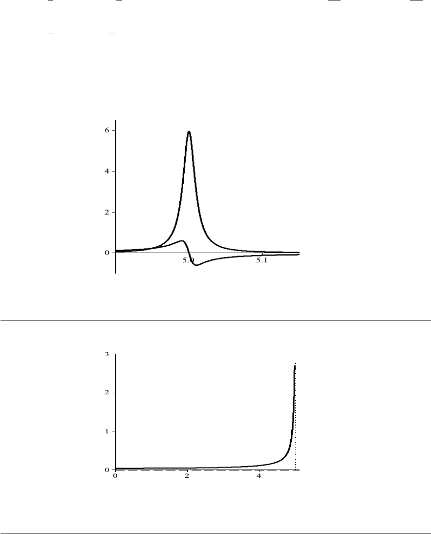
Figures
34. e
−7t
+ 4e
2t
36. −3e
−2t/3
+ te
−2t/3
38. y(t) =
−
1
4
cos 5t +
1
5
sin 5t, amplitude ≈ 0.320 m, period =
2π
5
, frequency=
5
2π
t
equilib
=
1
5
arctan
5
4
≈ 0.179 sec.
FIGURES
Figure 4–A: The graphs of A(Ω) and B(Ω) in Problem 10(b).
Figure 4–B: The graphs of A(Ω) and B(Ω) Problem 10(c).
173
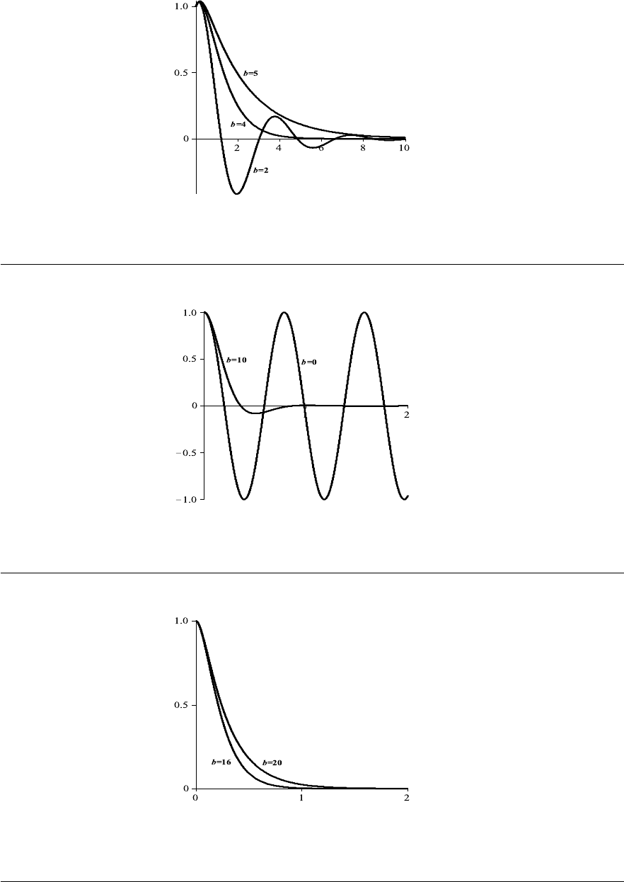
Chapter 4
Figure 4–C: The graphs of solutions in Problem 28 for b = 5, 4, and 2.
Figure 4–D: The graphs of the solutions in Problem 4 for b = 0, 10.
Figure 4–E: The graphs of the solutions in Problem 4 for b = 16, 20.
174
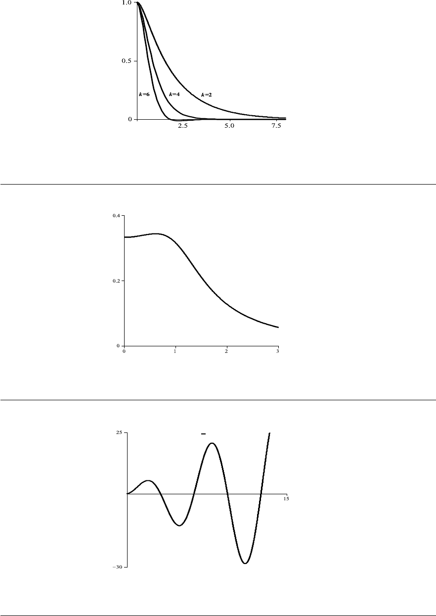
Figures
Figure 4–F: The graphs of the solutions in Problem 6 for k = 2, 4, and 6.
M(γ)
γ
Figure 4–G: The frequency response curve in Problem 2.
y = sin t +
5
2
t sin t
0 π 2π 3π 4π
Figure 4–H: The solution curve in Problem 4.
175
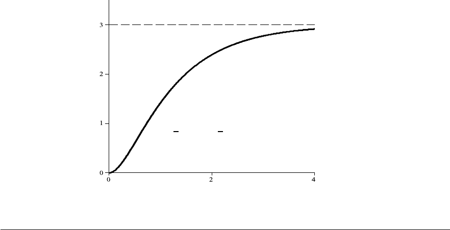
Chapter 4
y =
3
2
e
−3t
−
9
2
e
−t
+ 3
Figure 4–I: The solution curve in Problem 8.
176

CHAPTER 5: Introduction to Systems and
Phase Plane Analysis
EXERCISES 5.2: Elimination Method for Systems with Constant Coefficients
2. x =
3
2
c
1
e
2t
− c
2
e
−3t
;
y = c
1
e
2t
+ c
2
e
−3t
4. x = −
1
2
c
1
e
3t
+
1
2
c
2
e
−t
;
y = c
1
e
3t
+ c
2
e
−t
6. x =
c
1
+ c
2
2
e
t
cos 2t +
c
2
− c
1
2
e
t
sin 2t +
7
10
cos t −
1
10
sin t;
y = c
1
e
t
cos 2t + c
2
e
t
sin 2t +
11
10
cos t +
7
10
sin t
8. x = −
5c
1
4
e
11t
−
4
11
t −
26
121
;
y = c
1
e
11t
+
1
11
t +
45
121
10. x = c
1
cos t + c
2
sin t;
y =
c
2
− 3c
1
2
cos t −
c
1
+ 3c
2
2
sin t +
1
2
e
t
−
1
2
e
−t
12. u = c
1
e
2t
+ c
2
e
−2t
+ 1;
v = −2c
1
e
2t
+ 2c
2
e
−2t
+ 2t + c
3
14. x = −c
1
sin t + c
2
cos t + 2t − 1;
y = c
1
cos t + c
2
sin t + t
2
− 2
16. x = c
1
e
t
+ c
2
e
−2t
+
2
9
e
4t
;
y = −2c
1
e
t
−
1
2
c
2
e
−2t
+ c
3
−
1
36
e
4t
177

Chapter 5
18. x(t) = −t
2
− 4t − 3 + c
3
+ c
4
e
t
− c
1
te
t
−
1
2
c
2
e
−t
;
y(t) = −t
2
− 2t − c
1
e
t
+ c
2
e
−t
+ c
3
20. x(t) =
3
2
e
t
−
1
2
e
3t
;
y(t) = −
3
2
e
t
−
1
2
e
3t
+ e
2t
22. x(t) = 1 +
9
4
e
3t
−
5
4
e
−t
;
y(t) = 1 +
3
2
e
3t
−
5
2
e
−t
24. No solution
26. x =
1
2
e
t
[(c
1
− c
2
) cos t + (c
1
+ c
2
) sin t] + c
3
e
2t
;
y = e
t
(c
1
cos t + c
2
sin t);
z =
3
2
e
t
[(c
1
− c
2
) cos t + (c
1
+ c
2
) sin t] + c
3
e
2t
28. x(t) = c
1
+ c
2
e
−4t
+ 2c
3
e
3t
;
y(t) = 6c
1
− 2c
2
e
−4t
+ 3c
3
e
3t
;
z(t) = −13c
1
− c
2
e
−4t
− 2c
3
e
3t
30. λ ≤ 1
32. x =
20 − 10
√
19
√
19
!
e
(−7+
√
19)t/100
+
−20 − 10
√
19
√
19
!
e
(−7−
√
19)t/100
+ 20;
y =
−50
√
19
e
(−7+
√
19)t/100
+
50
√
19
e
(−7−
√
19)t/100
+ 20
34. (b) V
1
=
3
2
c
2
−
1
2
c
1
e
−t
cos 3t −
1
2
c
2
+
3
2
c
1
e
−t
sin 3t + 5L;
V
2
= c
1
e
−t
cos 3t + c
2
e
−t
sin 3t + 18L
(c) As t → +∞, V
1
→ 5L and V
2
→ 18L
36.
400
11
≈ 36.4
◦
F
38. A runaway arms race
178

Exercises 5.3
40. (a) 3x
2
= x
3
(b) 6x + 3x
2
− 2x
3
(c) 3x
2
+ 2x
3
;
(d) 6x + 3x
2
− 2x
3
(e) D
2
+ D − 2;
(f) 6x + 3x
2
− 2x
3
EXERCISES 5.3: Solving Systems and Higher–Order Equations Numerically
2. x
0
1
= x
2
,
x
0
2
= x
2
1
+ cos(t − x
1
);
x
1
(0) = 1, x
2
(0) = 0
4. x
0
1
= x
2
,
x
0
2
= x
3
,
x
0
3
= x
4
,
x
0
4
= x
5
,
x
0
5
= x
6
,
x
0
6
= x
2
2
− sin x
1
+ e
2t
;
x
1
(0) = . . . = x
6
(0) = 0
6. Setting x
1
= x, x
2
= x
0
, x
3
= y, x
4
= y
0
, we obtain
x
0
1
= x
2
,
x
0
2
= −
5
3
x
1
+
2
3
x
3
,
x
0
3
= x
4
,
x
0
4
=
3
2
x
1
−
1
2
x
3
8. x
1
(0) = a; x
2
(0) = p(0)b
10. See Table 5-A on page 185
12. See Table 5-B on page 185
179
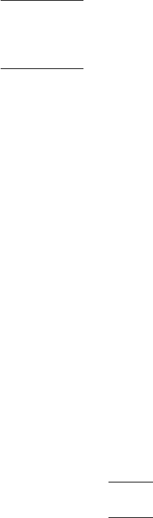
Chapter 5
14. y(8) ≈ 24.01531
16. x(1) ≈ 127.773; y(1) ≈ −423.476
18. Conventional troops
20. (a) period ≈ 2(3.14)
(b) period ≈ 2(3.20)
(c) period ≈ 2(3.34)
24. Yes; Yes
26. x(1) ≈ 0.80300; y(1) ≈ 0.59598; z(1) ≈ 0.82316
28. (a) x
0
1
= x
2
, x
1
(0) = 1
x
0
2
=
−x
1
(x
2
1
+ x
2
3
)
3/2
, x
2
(0) = 0
x
0
3
= x
4
, x
3
(0) = 0
x
0
4
=
−x
3
(x
2
1
+ x
2
3
)
3/2
, x
4
(0) = 1
(b) See Table 5-C on page 185
30. (a) See Table 5-D on page 186
(b) See Table 5-E on page 186
EXERCISES 5.4: Introduction to the Phase Plane
2. See Fig. 5–A on page 187
4. x = −6; y = 1
6. The line y = 2 and the point (1, 1)
8. x
3
− x
2
y − y
−2
= c
10. Critical points are (1, 0) and (−1, 0). Integral curves:
for y > 0, |x| > 1, y = c
√
x
2
− 1;
for y > 0, |x| < 1, y = c
√
1 − x
2
;
180

Exercises 5.4
for y < 0, |x| > 1, y = −c
√
x
2
− 1;
for y < 0, |x| < 1, y = −c
√
1 − x
2
; all with c ≥ 0
If c = 1, y = ±
√
1 − x
2
are semicircles ending at (1, 0) and (−1, 0)
12. 9x
2
+ 4y
2
= c. See Fig. 5–B on page 187
14. y = cx
2/3
See Fig. 5–C on page 187
16. (0, 0) is a stable node. See Fig. 5–D on page 188
18. (0, 0) is an unstable node;
(0, 5) is a stable no de;
(7, 0) is a stable no de;
(3, 2) is a saddle point;
See Fig. 5–E on page 188
20.
(
y
0
= v
v
0
= −y
(0, 0) is a center. See Fig. 5–F on page 189
22.
(
y
0
= v
v
0
= −y
3
(0, 0) is a center. See Fig. 5–G on page 189
24.
(
y
0
= v
v
0
= −y + y
3
(0, 0) is a center; (−1, 0) is a saddle point; (1, 0) is a saddle point. See Fig. 5–H on
page 190
26.
x
2
2
+
x
4
4
+
y
2
2
= c; all solutions are bounded. See Fig. 5–I on page 190
28. (0, 0) is a center; (1, 0) is a saddle point
30. (a) x → x
∗
, y → y
∗
, f and g are continuous implies x
0
(t) ≡ f (x(t), y(t)) → f (x
∗
, y
∗
)
and y
0
(t) ≡ g(x(t), y(t)) → g (x
,
y
∗
)
(b) x(t) =
t
Z
T
x
0
(τ)dτ + t(T ) >
f (x
∗
, y
∗
)
2
(t − T ) + x(T ) ≡ f (x
∗
, y
∗
)
t
2
+ C
181

Chapter 5
(c) If f (x
∗
, y
∗
) > 0, f(x
∗
, y
∗
)t → ∞ implying x(t) → ∞
(d) Similar
(e) Similar
32.
(y
0
)
2
2
+
y
4
4
= c by Problem 30. Thus,
y
4
4
= c −
(y
0
)
2
2
≤ c, so |y| ≤
4
√
4c
34. See Fig. 5–J on page 191
36. (a)
d
dt
x
2
+ y
2
+ z
2
= 0; the magnitude of the angular velocity is constant
(b) All points on the axes are critical points: (x, 0, 0), (0, y, 0), (0, 0, z)
(c) From (a), x
2
+ y
2
+ z
2
= K (sphere). Also
dy
dx
=
−2x
y
, so x
2
+
y
2
2
= c (cylinder)
(d) The solutions are periodic
(e) The critical point on the y-axis is unstable. The other two are stable
EXERCISES 5.5: Applications to Biomathematics: Epidemic and Tumor
Growth Models
2. 79.95mCi
EXERCISES 5.6: Coupled Mass–Spring Systems
2. x(t) =
√
10
20
!
1 −
√
10
cos r
1
t −
1 +
√
10
cos r
2
t
;
y(t) =
3
√
10
20
!
(cos r
1
t − cos r
2
t), where r
1
=
p
4 +
√
10 and r
2
=
p
4 −
√
10
4. m
1
x
00
= −k
1
x + k
2
(y − x);
m
2
y
00
= −k
2
(y − x) − by
0
6. (b) x(t) = c
1
cos t + c
2
sin t + c
3
cos 2t + c
4
sin 2t +
37
40
cos 3t
(c) y(t) = 2c
1
cos t + 2c
2
sin t − c
3
cos 2t − c
4
sin 2t −
111
20
cos 3t
(d) x(t) =
23
8
cos t −
9
5
cos 2t +
37
40
cos 3t;
y(t) =
23
4
cos t +
9
5
cos 2t −
111
20
cos 3t
182

Exercises 5.8
8. θ
1
(t) =
π
12
cos
s
9.8
5 +
√
10
t
!
+
π
12
cos
s
9.8
5 −
√
10
t
!
;
θ
2
(t) =
π
√
10
24
cos
s
9.8
5 +
√
10
t
!
−
π
√
10
24
cos
s
9.8
5 −
√
10
t
!
EXERCISES 5.7: Electrical Systems
2. q (t) =
1
2
e
−4t
cos 6t + 3 cos 2t + sin 2t coulombs
4. I (t) =
10
33
cos 5t −
10
33
cos 50t amps
8. L = 0.01 henrys, R = 0.2 ohms, C =
25
32
farads, and E (t) =
2
5
cos 8t volts
10. I
1
= −
1
4
e
−2t
−
9
4
e
−2t/3
+
5
2
;
I
2
=
1
4
e
−2t
−
3
4
e
−2t/3
+
1
2
;
I
3
= −
1
2
e
−2t
−
3
2
e
−2t/3
+ 2
12. I
1
= 1 − e
−900t
; I
2
=
5
9
−
5
9
e
−900t
; I
3
=
4
9
−
4
9
e
−900t
EXERCISES 5.8: Dynamical Systems, Poincar`e Maps, and Chaos
2. (x
0
, v
0
) = (−1.5, 0.5774)
(x
1
, v
1
) = (−1.9671, −0.5105)
(x
2
, v
2
) = (−0.6740, 0.3254)
.
.
.
(x
20
, v
20
) = (−1.7911, −0.5524)
The limit set is the ellipse (x + 1.5)
2
+ 3v
2
= 1
4. (x
0
, v
0
) = (0, 10.9987)
(x
1
, v
1
) = (−0.00574, 10.7298)
(x
2
, v
2
) = (−0.00838, 10.5332)
183

Chapter 5
.
.
.
(x
20
, v
20
) = (−0.00029, 10.0019)
The attractor is the point (0, 10)
12. For F = 0.2, the attractor is the point (−0.319, −0.335). For F = 0.28, the attractor is
the point (−0.783, 0.026)
14. The attractor consists of two points: (−1.51, 0.06) and (−0.22, −0.99). See Fig. 5–K on
page 191
REVIEW PROBLEMS
2. x = −(c
1
+ c
2
) e
−t
cos 2t + (c
1
− c
2
) e
−t
sin 2t;
y = 2c
1
e
−t
cos 2t + 2c
2
e
−t
sin 2t
4. x = c
1
t + c
2
+ e
−t
; y =
1
6
c
1
t
3
+
1
2
c
2
t
2
+ c
3
t + c
4
6. x = e
2t
+ e
−t
; y = e
2t
+ e
−t
; z = e
2t
− 2e
−t
8. With x
1
= y, x
2
= y
0
, we obtain x
0
1
= x
2
, x
0
2
=
1
2
(sin t − 8x
1
+ tx
2
)
10. With x
1
= x, x
2
= x
0
, x
3
= y, x
4
= y
0
, we get x
0
1
= x
2
, x
0
2
= x
1
− x
3
, x
0
3
= x
4
,
x
0
4
= −x
2
+ x
3
12. Solutions to the phase plane equation
dy
dx
=
2 − x
y − 2
are given implicitly by the equation
(x − 2)
2
+ (y − 2)
2
= const. Critical point is at (2, 2), which is a stable center. See
Fig. 5–L on page 192
14. Critical points are (mπ, nπ) (m, n integers) and
(2j + 1) π
2
,
(2k + 1) π
2
(j, k integers).
Equation for integral curves is
dy
dx
=
cos x sin y
sin x cos y
=
tan y
tan x
, with solutions sin y = C sin x
16. Origin is a saddle(unstable) See Fig. 5–M on page 192
18. Natural angular frequencies are
√
2, 2
√
3.
General solution is x(t) = c
1
cos
2
√
3t
+ c
2
sin
2
√
3t
+ c
3
cos
√
2t
+ c
4
sin
√
2t
;
y(t) = −
1
3
c
1
cos
2
√
3t
−
1
3
c
2
sin
2
√
3t
+ 3c
3
cos
√
2t
+ 3c
4
sin
√
2t
184
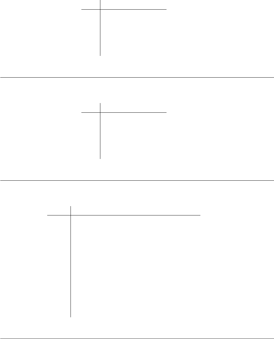
Tables
TABLES
i t
i
y(t
i
)
1 0.250 0.96924
2 0.500 0.88251
3 0.750 0.75486
4 1.000 0.60656
Table 5–A: Approximations to the solution in Problem 10.
i t
i
y(t
i
)
1 1.250 0.80761
2 1.500 0.71351
3 1.750 0.69724
4 2.000 0.74357
Table 5–B: Approximations to the solution in Problem 12.
i t
i
x
1
(t
i
) ≈ x(t
i
) x
3
(t
i
) ≈ y(t
i
)
10 0.628 0.80902 0.58778
20 1.257 0.30902 0.95106
30 1.885 −0.30902 0.95106
40 2.513 0.80902 0.58779
50 3.142 −1.00000 0.00000
60 3.770 −0.80902 −0.58778
70 4.398 −0.30903 −0.95106
80 5.027 0.30901 −0.95106
90 5.655 0.80901 −0.58780
100 6.283 1.00000 −0.00001
Table 5–C: Approximations to the solution in Problem 28.
185

Chapter 5
t
i
l
i
θ
i
1.0 5.27015 0.0
2.0 4.79193 0.0
3.0 4.50500 0.0
4.0 4.67318 0.0
5.0 5.14183 0.0
6.0 5.48008 0.0
7.0 5.37695 0.0
8.0 4.92725 0.0
9.0 4.54444 0.0
10.0 4.58046 0.0
Table 5–D: Approximations to the solution in Problem 30(a).
t
i
l
i
θ
i
1.0 5.13916 0.45454
2.0 4.10579 0.28930
3.0 2.89358 −0.10506
4.0 2.11863 −0.83585
5.0 2.13296 −1.51111
6.0 3.18065 −1.64163
7.0 5.10863 −1.49843
8.0 6.94525 −1.29488
9.0 7.76451 −1.04062
10.0 7.68681 −0.69607
Table 5–E: Approximations to the solution in Problem 30(b).
186
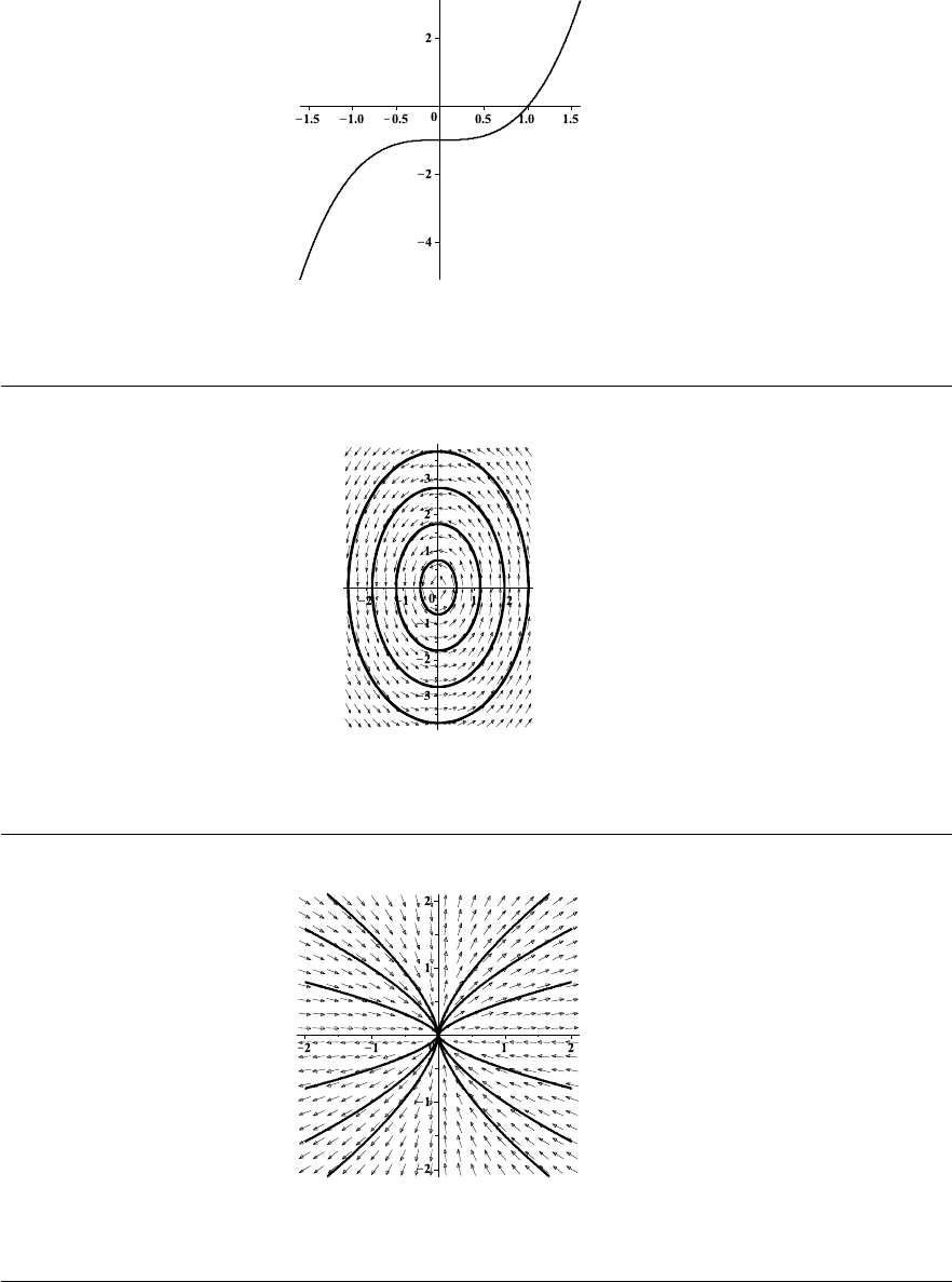
Figures
FIGURES
Figure 5–A: Problem 2, Section 5.4
Figure 5–B: Problem 12, Section 5.4
Figure 5–C: Problem 14, Section 5.4
187
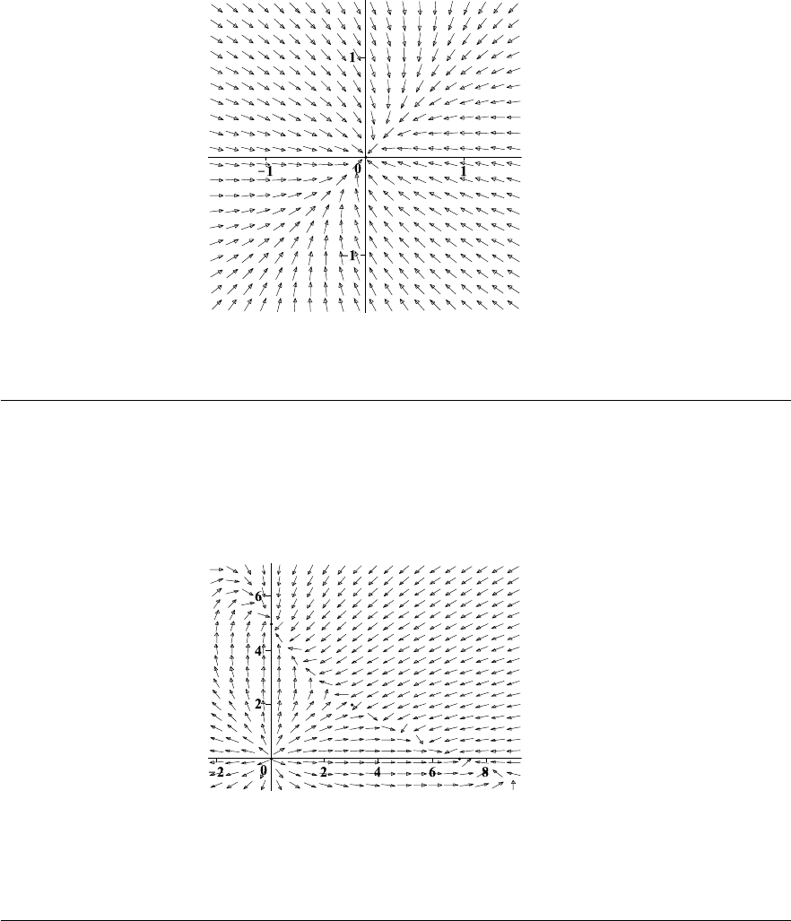
Chapter 5
Figure 5–D: Problem 16, Section 5.4
Figure 5–E: Problem 18, Section 5.4
188

Figures
Figure 5–F: Problem 20, Section 5.4
Figure 5–G: Problem 22, Section 5.4
189
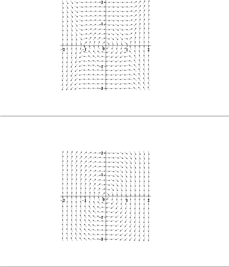
Chapter 5
Figure 5–H: Problem 24, Section 5.4
Figure 5–I: Problem 26, Section 5.4
190
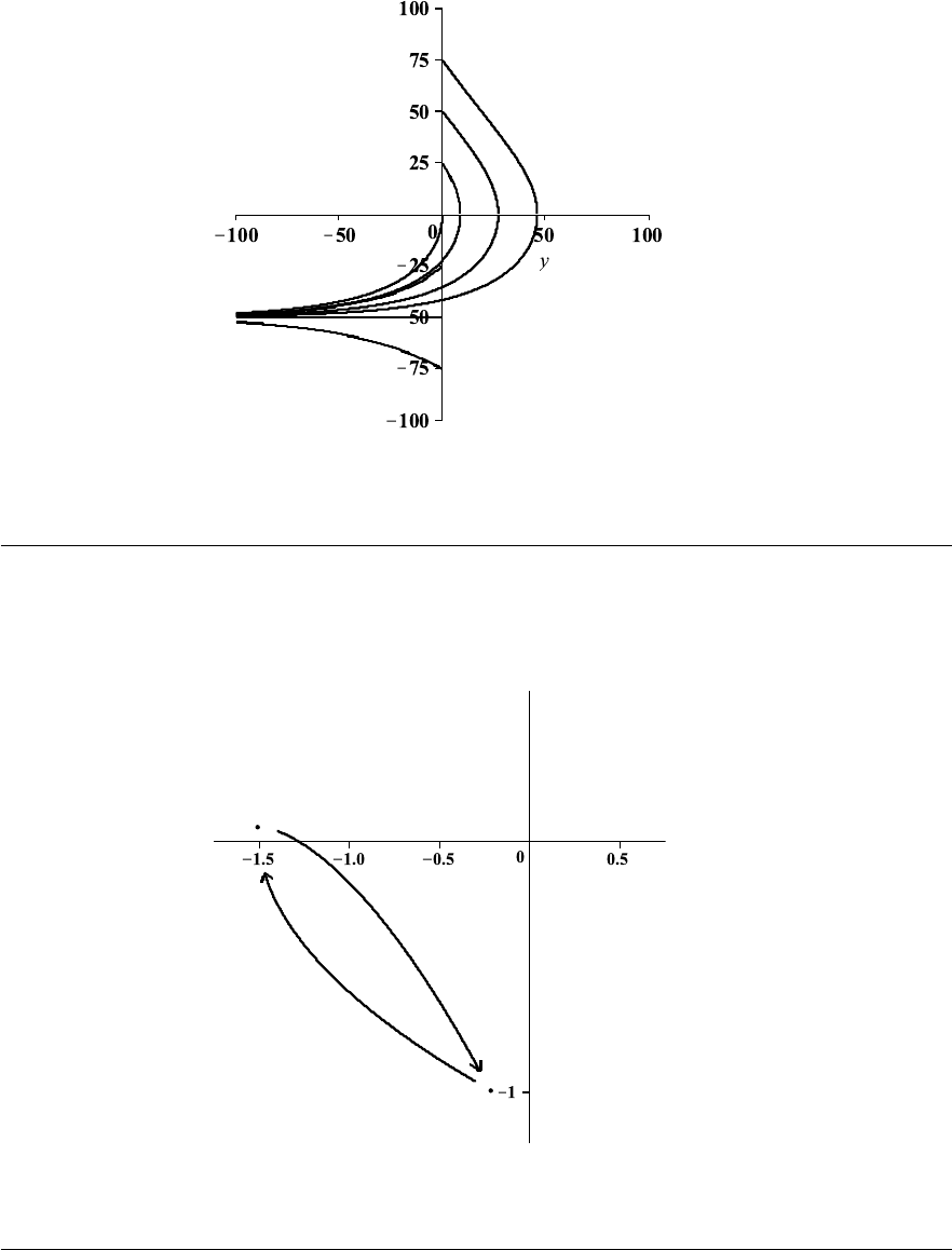
Figures
Figure 5–J: Problem 34, Section 5.4
Figure 5–K: Problem 14, Section 5.8
191
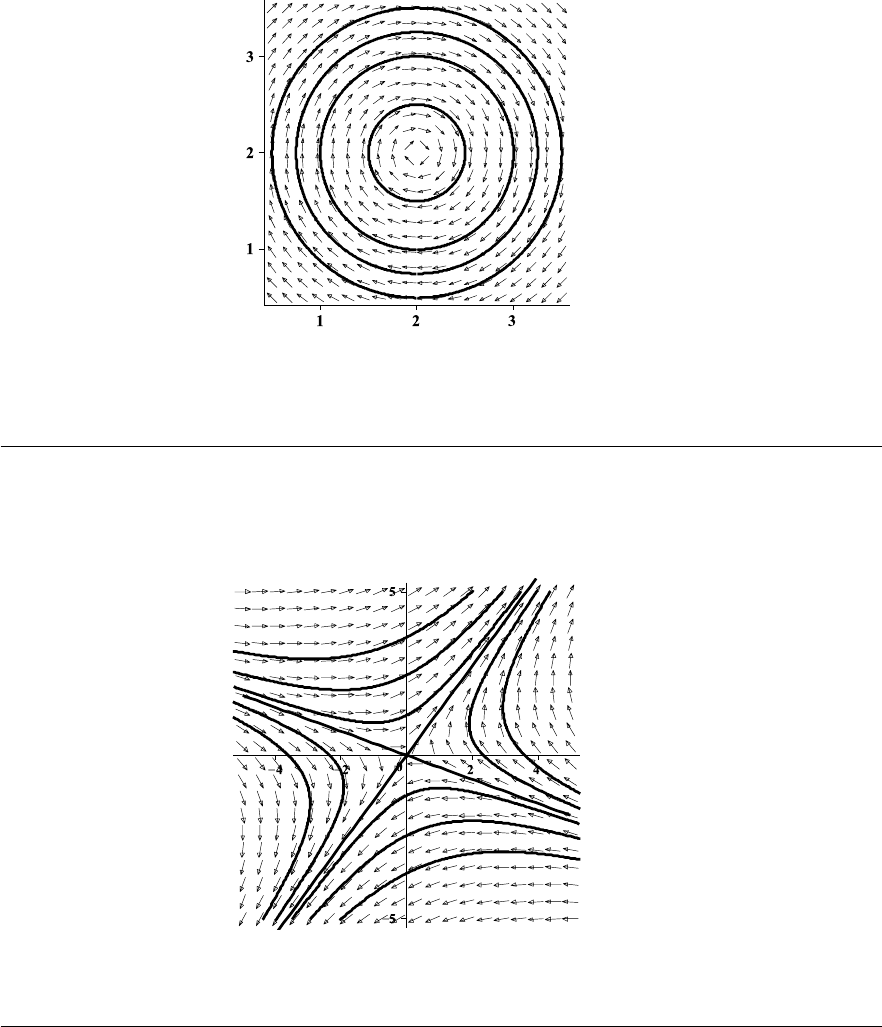
Chapter 5
Figure 5–L: Problem 12, Review Problems
Figure 5–M: Problem 16, Review Problems
192
CHAPTER 6: Theory of Higher-Order Linear
Differential Equations
EXERCISES 6.1: Basic Theory of Linear Differential Equations
2. (0, ∞)
4. (−1, 0)
6. (0, 1)
8. Linearly dependent; 0
10. Linearly independent; −2 tan
3
x − sin x cos x − sin
2
x tan x − 2 tan x
12. Linearly dependent; 0
14. Linearly independent; (x + 2)e
x
16. c
1
e
x
+ c
2
cos 2x + c
3
sin 2x
18. c
1
e
x
+ c
2
e
−x
+ c
3
cos x + c
4
sin x
20. (a) c
1
+ c
2
x + c
3
x
3
+ x
2
(b) 2 − x
3
+ x
2
22. (a) c
1
e
x
cos x + c
2
e
x
sin x + c
3
e
−x
cos x + c
4
e
−x
sin x + cos x
(b) e
x
cos x + cos x
24. (a) 7 cos 2x + 1
(b) −6 cos 2x − (11/3)
26. y(x) =
P
n+1
j=1
γ
j−1
y
j
(x)
34. The coefficient is the Wronskian W [f
1
, f
2
, f
3
] (x)
193

Chapter 6
EXERCISES 6.2: Homogeneous Linear Equations with Constant Coefficients
2. c
1
e
x
+ c
2
e
−x
+ c
3
e
3x
4. c
1
e
−x
+ c
2
e
−5x
+ c
3
e
4x
6. c
1
e
−x
+ c
2
e
x
cos x + c
3
e
x
sin x
8. c
1
e
x
+ c
2
xe
x
+ c
3
e
−7x
10. c
1
e
−x
+ c
2
e
(
−1+
√
7
)
x
+ c
3
e
(
−1−
√
7
)
x
12. c
1
e
x
+ c
2
e
−3x
+ c
3
xe
−3x
14. c
1
sin x + c
2
cos x + c
3
e
−x
+ c
4
xe
−x
16. (c
1
+ c
2
x) e
−x
+ (c
3
+ c
4
x + c
5
x
2
) e
6x
+ c
6
e
−5x
+ c
7
cos x + c
8
sin x + c
9
cos 2x + c
10
sin 2x
18. (c
1
+ c
2
x + c
3
x
2
) e
x
+ c
4
e
2x
+ c
5
e
−x/2
cos
√
3x/2
+ c
6
e
−x/2
sin
√
3x/2
+ (c
7
+ c
8
x + c
9
x
2
) e
−3x
cos x + (c
10
+ c
11
x + c
12
x
2
) e
−3x
sin x
20. e
−x
− e
−2x
+ e
−4x
22. x(t) = c
1
e
√
3t
+ c
2
e
−
√
3t
+ c
3
cos 2t + c
4
sin 2t,
y(t) = −(2c
1
/5) e
√
3t
− (2c
2
/5) e
−
√
3t
+ c
3
cos 2t + c
4
sin 2t
28. c
1
e
1.879x
+ c
2
e
−1.532x
+ c
3
e
−0.347x
34. x(t) =
5 −
√
10
10
!
cos
q
4 +
√
10 t +
5 +
√
10
10
!
cos
q
4 −
√
10 t,
y(t) =
5 − 2
√
10
10
!
cos
q
4 +
√
10 t +
5 + 2
√
10
10
!
cos
q
4 −
√
10 t
EXERCISES 6.3: Undetermined Coefficients and the Annihilator Method
2. c
1
e
−x
+ c
2
cos x + c
3
sin x
4. c
1
+ c
2
xe
x
+ c
3
x
2
e
x
6. c
1
e
x
+ c
2
xe
x
+ c
3
e
−3x
+ (1/8)e
−x
+ (3/20) cos x + (1/20) sin x
8. c
1
e
x
+ c
2
e
−x
cos x + c
3
e
−x
sin x − (1/2) − (4/25)xe
x
+ (1/10)x
2
e
x
194

Exercises 6.4
10. c
1
e
2x
+ c
2
e
−3x
cos 2x + c
3
e
−3x
sin 2x + (5/116)xe
−3x
cos 2x − (1/58)xe
−3x
sin 2x
− (1/26)x − (1/676)
12. D
3
14. D − 5
16. D
3
(D − 1)
18. [(D − 3)
2
+ 25]
2
20. D
4
(D − 1)
3
(D
2
+ 16)
2
22. c
1
e
3x
+ c
2
cos x + c
3
sin x
24. c
1
xe
x
+ c
2
x
2
e
x
26. c
1
x
2
+ c
2
x + c
3
28. c
1
e
3x
+ c
2
+ c
3
x
30. c
1
xe
x
+ c
2
32. 5 + e
x
sin 2x − e
3x
38. x(t) = {c
1
+ (1/2) + (1/4)t}e
t
−
(3/2)c
2
+
√
7/2
c
3
e
−t/2
cos
√
7 t/2
+
√
7/2
c
2
− (3/2)c
3
e
−t/2
sin
√
7 t/2
+ t + 1,
y(t) = {c
1
+ (1/4)t}e
t
+ c
2
e
−t/2
cos
√
7 t/2
+ c
3
e
−t/2
sin
√
7 t/2
+ (1/2)
40. I
1
(t) = (2187/40) sin(t/8) −(3/40) sin(t/72) − 18 sin(t/24),
I
2
(t) = (243/40) sin(t/8) −(27/40) sin(t/72),
I
3
(t) = (243/5) sin(t/8) + (3/5) sin(t/72) − 18 sin(t/24)
EXERCISES 6.4: Method of Variation of Parameters
2. (1/2)x
2
+ 2x
4. (1/6)x
3
e
x
6. sec θ − sin θ tan θ + θ sin θ + (cos θ) ln(cos θ)
195
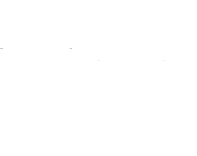
Chapter 6
8. c
1
x + c
2
x ln x + c
3
x
3
− x
2
10. 1/(10x)
R
g(x)dx + (x
4
/15)
R
x
−5
g(x)dx − (x/6)
R
x
−2
g(x)dx
REVIEW PROBLEMS
2. (a) Linearly independent.
(b) Linearly independent.
(c) Linearly dependent.
4. (a) c
1
e
−3x
+ c
2
e
−x
+ c
3
e
x
+ c
4
xe
x
(b) c
1
e
x
+ c
2
e
(
−2+
√
5
)
x
+ c
3
e
(
−2−
√
5
)
x
(c) c
1
e
x
+ c
2
cos x + c
3
sin x + c
4
x cos x + c
5
x sin x
(d) c
1
e
x
+ c
2
e
−x
+ c
3
e
2x
− (x/2)e
x
+ (x/2) + (1/4)
6. c
1
e
−x/
√
2
cos
x/
√
2
+ c
2
e
−x/
√
2
sin
x/
√
2
+ c
3
e
x/
√
2
cos
x/
√
2
+ c
4
e
x/
√
2
sin
x/
√
2
+ sin (x
2
)
8. (a) c
1
xe
−x
+ c
2
+ c
3
x + c
4
x
2
(b) c
1
xe
−x
+ c
2
x
2
e
−x
(c) c
1
+ c
2
x + c
3
x
2
+ c
4
cos 3x + c
5
sin 3x
(d) c
1
cos x + c
2
sin x + c
3
x cos x + c
4
x sin x
10. (a) c
1
x
1/2
+ c
2
x
−1/2
+ c
3
x
(b) c
1
x
−1
+ c
2
x cos
√
3 ln x
+ c
3
x sin
√
3 ln x
196

CHAPTER 7: Laplace Transforms
EXERCISES 7.2: Definition of the Laplace Transform
2. For s > 0, using Definition and integration by parts twice, we compute
L
t
2
(s) =
∞
Z
0
e
−st
t
2
dt = lim
N→∞
N
Z
0
e
−st
t
2
dt
= lim
N→∞
−
t
2
e
−st
s
N
0
+
2
s
N
Z
0
te
−st
dt
= lim
N→∞
−
t
2
s
−
2t
s
2
−
2
s
3
e
−st
N
0
= lim
N→∞
2
s
3
−
N
2
s
+
2N
s
2
+
2
s
3
e
−sN
=
2
s
3
,
because, for s > 0 and any k, N
k
e
−sN
→ 0 as N → ∞.
4. For s > 3, we have
L
te
3t
(s) =
∞
Z
0
e
−st
te
3t
dt =
∞
Z
0
te
(3−s)t
dt = lim
N→∞
N
Z
0
te
(3−s)t
dt
= lim
N→∞
t
3 − s
−
1
(3 − s)
2
e
(3−s)t
N
0
= lim
N→∞
1
(3 − s)
2
+
N
3 − s
−
1
(3 − s)
2
e
(3−s)N
=
1
(s − 3)
2
.
6. Referring to the table of integrals on the inside front cover, we see that, for s > 0,
L{cos bt}(s) =
∞
Z
0
e
−st
cos bt dt = lim
N→∞
N
Z
0
e
−st
cos bt dt
= lim
N→∞
e
−st
(−s cos bt + b sin bt)
s
2
+ b
2
N
0
= lim
N→∞
e
−sN
(−s cos bN + b sin bN)
s
2
+ b
2
−
−s
s
2
+ b
2
=
s
s
2
+ b
2
,
where we have used integration by parts to find an antiderivative of e
−st
cos 2t.
197

Chapter 7
8. For s > −1,
L
e
−t
sin 2t
(s) =
∞
Z
0
e
−st
e
−t
sin 2t dt =
∞
Z
0
e
−(s+1)t
sin 2t dt
= lim
N→∞
e
−(s+1)t
(−(s + 1) sin 2t − 2 cos 2t)
(s + 1)
2
+ 4
N
0
= lim
N→∞
e
−(s+1)N
[−(s + 1) sin 2N − 2 cos 2N] + 2)
(s + 1)
2
+ 4
=
2
(s + 1)
2
+ 4
.
10. In this problem, f(t) is also a piecewise defined function. So, we split the integral and
obtain
L{f(t)}(s) =
∞
Z
0
e
−st
f(t) dt =
1
Z
0
e
−st
(1 − t) dt +
∞
Z
1
e
−st
· 0 dt =
1
Z
0
(1 − t)e
−st
dt
=
−
1 − t
s
+
1
s
2
e
−st
1
0
=
e
−s
s
2
+
1
s
−
1
s
2
,
which is valid for all s.
12. Splitting the integral in the definition of Laplace transform, we get
L{f(t)}(s) =
∞
Z
0
e
−st
f(t) dt =
3
Z
0
e
−st
e
2t
dt +
∞
Z
3
e
−st
· 1 dt
=
e
(2−s)t
2 − s
3
0
−
e
−st
s
∞
3
=
1 − e
−3(s−2)
s − 2
+
e
−3s
s
,
which is valid for all s > 2.
14. By the linearity of the Laplace transform,
L
5 − e
2t
+ 6t
2
(s) = 5L{1}(s) −L
e
2t
(s) + 6L
t
2
(s).
From Table 7.1 in the text, we see that
L{1}(s) =
1
s
, s > 0,
L
e
2t
(s) =
1
s − 2
, s > 2,
L
t
2
(s) =
2!
s
2+1
=
2
s
3
, s > 0.
Thus, the formula
L
5 − e
2t
+ 6t
2
(s) =
5
s
−
1
s − 2
+
12
s
3
is valid for s in the intersection of the sets s > 2 and s > 0, which is s > 2.
198

Exercises 7.2
16. Using the linearity of Laplace transform and Table 7.1 in the text, we get
L
t
2
− 3t − 2e
−t
sin 3t
(s) = L
t
2
(s) − 3L{t}(s) − 2L
e
−t
sin 3t
(s)
=
2!
s
2+1
− 3
1!
s
1+1
− 2
3
(s + 1)
2
+ 3
2
=
2
s
3
−
3
s
2
−
6
(s + 1)
2
+ 9
,
valid for s > 0.
18. Using the linearity of Laplace transform and Table 7.1, we get
L
n
t
4
− t
2
− t + sin
√
2t
o
= L
t
4
− L
t
2
− L{t} + L
n
sin
√
2t
o
=
4!
s
4+1
−
2!
s
2+1
−
1!
s
1+1
+
√
2
s
2
+
√
2
2
=
24
s
5
−
2
s
3
−
1
s
2
+
√
2
s
2
+ 2
,
valid for s > 0.
20. For s > −2, we have
L
n
e
−2t
cos
√
3t − t
2
e
−2t
o
(s) = L
n
e
−2t
cos
√
3t
o
(s) − L
t
2
e
−2t
(s)
=
s + 2
(s + 2)
2
+ (
√
3)
2
−
2!
(s + 2)
2+1
=
s + 2
(s + 2)
2
+ 3
−
2
(s + 2)
3
.
22. Since the function g
1
(t) ≡ 0 is continuous on (−∞, ∞) and f(t) = g
1
(t) for t in [0, 2),
we conclude that f(t) is continuous on [0, 2) and continuous from the left at t = 1. The
function g
2
(t) ≡ t is also continuous on (−∞, ∞), and so f(t) (which is the same as
g
2
(t) on [2, 10]) is continuous on (2, 10]. Since
lim
t→2
−
f(t) = 0 6= 2 lim
t→2
+
f(t),
f(t) has a jump discontinuity at t = 2. Thus f(t) is piecew ise continuous on [0, 10]. The
graph of f(t) is depicted in Fig. 7–A on page 263.
24. Given function is a rational function and, therefore, continuous on its domain, which
is all reals except zeros of the denominator. Solving t
2
− 4 = 0, we conclude that the
199
Chapter 7
points of discontinuity of f(t) are t = ±2. The point t = −2 is not in [0, 10], and
lim
t→2
f(t) = lim
t→2
t
2
− 3t + 2
t
2
− 4
= lim
t→2
(t − 2)(t − 1)
(t − 2)(t + 2)
= lim
t→2
t − 1
t + 2
=
1
4
.
Therefore, f(t) has a removable singularity at t = 2, and it is piecewise continuous on
[0, 10]. The graph of f(t) is shown in Fig. 7–B on page 263.
26. Since
lim
t→1
+
f(t) = lim
t→1
+
t
t
2
− 1
= +∞,
f(t) has an infinite discontinuity at t = 1, and it is so neither continuous nor piecewise
continuous [0, 10]. The graph of f(t) is depicted in Fig. 7–C on page 263.
28. This function is continuous everywhere except, possibly, t = 0. Using L’Hospital’s rule,
we see that
lim
t→0
f(t) = lim
t→0
sin t
t
= lim
t→0
cos t
1
= 1 = f(1).
Therefore, f(t) is continuous at t = 0 as well, and so it is continuous on (−∞, ∞). The
graph of f(t) is given in Fig. 7–D on page 264.
30. All the Laplace transforms F (s) in Table 7.1 are proper rational functions, that is, the
degree of the numerator is less than the degree of the denominator. Therefore,
lim
s→∞
F (s) = 0.
32. This statement is a consequence of the following more general result.
If lim
t→∞
f(t) = 0 and, for some T , |g(t)| ≤ M for t ≥ T , then lim
t→∞
f(t)g(t) = 0.
Indeed, for t ≥ T , one has
0 ≤ |f(t)g(t)| ≤ M|f(t)| → 0, as t → ∞.
Therefore, by the squeeze theorem,
lim
t→∞
|f(t)g(t)| = 0 ⇔ lim
t→∞
f(t)g(t) = 0.
In the given problem, we take f (t) = e
−st
and g(t) = s sin bt + b cos bt. Then f(t) → 0,
as t → ∞, because s > 0 and g(t) is bounded (by s + |b|).
200

Exercises 7.3
EXERCISES 7.3: Properties of the Laplace Transform
2. Using the linearity of the Laplace transform, we get
L
3t
2
− e
2t
(s) = 3L
t
2
(s) − L
e
2t
(s).
From Table 7.1 in Section 7.2 we know that
L
t
2
(s) =
2!
s
3
=
2
s
3
, L
e
2t
(s) =
1
s − 2
.
Thus
L
3t
2
− e
2t
(s) = 3
2
s
3
−
1
s − 2
=
6
s
3
−
1
s − 2
.
4. By the linearity of the Laplace transform,
L
3t
4
− 2t
2
+ 1
(s) = 3L
t
4
(s) − 2L
t
2
(s) + L{1}(s).
From Table 7.1 of the text we see that
L
t
4
(s) =
4!
s
5
, L
t
2
(s) =
2!
s
3
, L{1}(s) =
1
s
, s > 0.
Therefore,
L
3t
4
− 2t
2
+ 1
(s) = 3
4!
s
5
− 2
2!
s
3
+
1
s
=
72
s
5
−
4
s
3
+
1
s
,
is valid for s > 0.
6. We use the linearity of the Laplace transform and Table 7.1 to get
L
e
−2t
sin 2t + e
3t
t
2
(s) = L
e
−2t
sin 2t
(s) + L
e
3t
t
2
(s)
=
2
(s + 2)
2
+ 4
+
2
(s − 3)
3
, s > 3.
8. Since (1 + e
−t
)
2
= 1 + 2e
−t
+ e
−2t
, we have from the linearity of the Laplace transform
that
L
(1 + e
−t
)
2
(s) = L{1}(s) + 2L
e
−t
(s) + L
e
−2t
(s).
From Table 7.1 of the text, we get
L{1}(s) =
1
s
, L
e
−t
(s) =
1
s + 1
, L
e
−2t
(s) =
1
s + 2
.
Thus
L
(1 + e
−t
)
2
(s) =
1
s
+
2
s + 1
+
1
s + 2
, s > 0.
201

Chapter 7
10. Since
L
e
2t
cos 5t
(s) =
s − 2
(s − 2)
2
+ 25
,
we use Theorem 6 to get
L
te
2t
cos 5t
(s) = L
t
e
2t
cos 5t
(s) = −
L
e
2t
cos 5t
(s)
0
= −
s − 2
(s − 2)
2
+ 25
0
= −
[(s − 2)
2
+ 25] − (s − 2) · 2(s − 2)
[(s − 2)
2
+ 25]
2
=
(s − 2)
2
− 25
[(s − 2)
2
+ 25]
2
.
12. Since sin 3t cos 3t = (1/2) sin 6t, we obtain
L{sin 3t cos 3t}(s) =
1
2
L{sin 6t}(s) =
1
2
6
s
2
+ 6
2
=
3
s
2
+ 36
.
14. In this problem, we need the trigonometric identity sin
2
t = (1 − cos 2t)/2 and the
linearity of the Laplace transform.
L
e
7t
sin
2
t
(s) = L
e
7t
1 − cos 2t
2
(s) =
1
2
L
e
7t
(s) − L
e
7t
cos 2t
(s)
=
1
2
1
s − 7
−
s − 7
(s − 7)
2
+ 4
=
2
(s − 7)[(s − 7)
2
+ 4]
.
16. Since
t sin
2
t =
t(1 − cos 2t)
2
,
we write
L
t sin
2
t
(s) =
1
2
[L{t}(s) − L{t cos 2t}(s)]
=
1
2
1
s
2
+
s
s
2
+ 4
0
=
1
2
1
s
2
+
4 − s
2
(s
2
+ 4)
2
,
which holds for s > 0.
18. Since cos A cos B = [cos(A −B) + cos(A + B)]/2, we get
L{cos nt cos mt}(s) = L
cos(n − m)t + cos(n + m)t
2
(s)
=
1
2
[L{cos(n − m)t}(s) + L{cos(n + m)t}(s)]
=
1
2
s
s
2
+ (n − m)
2
+
s
s
2
+ (n + m)
2
=
s(s
2
+ n
2
+ m
2
)
[s
2
+ (n − m)
2
][s
2
+ (n + m)
2
]
.
202

Exercises 7.3
20. Since sin A sin B = [cos(A − B) − cos(A + B)]/2, using the linearity of the Laplace
transform and Theorem 6, we get
L{t sin 2t sin 5t}(s) = −
d
ds
L
cos 3t − cos 7t
2
(s) = −
1
2
d
ds
s
s
2
+ 9
−
s
s
2
+ 49
= −20
s
(s
2
+ 9)(s
2
+ 49)
0
=
20(3s
4
+ 58s
2
− 441)
(s
2
+ 9)
2
(s
2
+ 49)
2
.
22. We represent t
n
= t
n
· 1 and apply (6) to get
L{t
n
}(s) = L{t
n
· 1}(s) = (−1)
n
d
n
ds
n
[L{1}(s)] = (−1)
n
d
n
(s
−1
)
ds
n
= (−1)
n
(−1)(−2) ···(−n)s
−1−n
=
(−1)
n
(−1)
n
1 · 2 ···n
s
n+1
=
n!
s
n+1
.
24. (a) Applying (1), the “translation in s” property of the Laplace transform, to f(t) = t
n
yields
L
e
at
t
n
(s) = L{t
n
}(s − a) =
n!
(s − a)
n+1
, s > a .
(b) We apply (6) to the Laplace transform of f(t) = e
at
, which is of exponential order
a.
L
t
n
e
at
(s) = (−1)
n
d
n
ds
n
L
e
at
(s)
= (−1)
n
d
n
[(s − a)
−1
]
ds
n
= (−1)
n
(−1)(−2) ···(−n)(s − a)
−1−n
=
n!
(s − a)
n+1
, s > a .
26. (a) By Definition 3, there exist constants M, T , and α such that
|f(t)| ≤ Me
αt
for t ≥ T.
Since f(t) is piecewise continuous on [0, T ], there exists a finite number of points
0 = t
0
< t
1
< ··· < t
n
= T
such that f(t) is continuous on each (t
j
, t
j+1
) and has finite one-sided limits at
endpoints. This implies that f(t) is bounded on any closed subinterval of (t
j−1
, t
j
),
and bounded near the endpoints. Thus,
|f(t)| ≤ M
j
on (t
j
, t
j+1
) , j = 0, 1, . . . n − 1.
Therefore,
|f(t)| ≤ N = max
0≤j<n
{M
j
, f (t
j
)} 0 ≤ t < T,
203

Chapter 7
and so
|f(t)| ≤
Ne
−αt
e
αt
≤ sup
0≤t≤T
Ne
−αt
e
αt
= Le
αt
on [0, T ).
Hence, on [0, ∞),
|f(t)| ≤ max{L, M}e
αt
= Ke
αt
.
(b) For s > α, we have
0 ≤ |L{f(t)}(s)| =
∞
Z
0
f(t)e
−st
dt
≤
∞
Z
0
|f(t)|e
−st
dt
≤
∞
Z
0
Ke
αt
e
−st
dt = K
∞
Z
0
e
(α−s)t
dt =
K
α −s
e
(α−s)t
t=∞
t=0
=
K
s − α
.
Since
lim
s→∞
K
s − α
= 0,
by the squeeze theorem
lim
s→∞
|L{f(t)}(s)| = 0,
which is equivalent to
lim
s→∞
L{f(t)}(s) = 0.
28. First observe that since both functions f(t) are continuous on [0, ∞), of exponential
order α for any α > 0, and f(t)/t → 0 as t → 0
+
. Thus, the formula in Problem 27
applies.
(a) From Table 1,
F (s) = L
t
5
(s) =
5!
s
6
= 5!s
−6
⇒
∞
Z
s
F (u)du = 5!
∞
Z
s
u
−6
du =
5!
−5
u
−5
∞
s
=
4!
s
5
= L
t
4
(s) = L
t
5
t
(s) .
(b) Here, we use (21) on the inside back cover with n = 2 to conclude that
F (s) = L
t
3/2
(s) =
3
√
π
4s
5/2
=
3
√
π
4
s
−5/2
⇒
∞
Z
s
F (u)du =
3
√
π
4
∞
Z
s
u
−5/2
du =
3
√
π
4
·
−2
3
u
−3/2
∞
s
204

Exercises 7.3
=
√
π
2s
3/2
= L
t
1/2
(s) = L
t
3/2
t
(s) .
30. From the linearity properties (2) and (3) of the text we have
L{g}(s) = L{y
00
+ 5y
0
+ 6y}(s) = L{y
00
}(s) + 5L{y
0
}(s) + 6L{y}(s).
Next, applying properties (2) and (4) yields
L{g}(s) =
s
2
L{y}(s) −sy(0) − y
0
(0)
+ 5 [sL{y}(s) −y(0)] + 6L{y}(s).
Keeping in mind the fact that b oth initial values are zero, we get
G(s) =
s
2
+ 6s + 10
Y (s), where G(s) = L{g}(s), Y (s) = L{y}(s).
Therefore, the transfer function H(s) is given by
H(s) =
Y (s)
G(s)
=
1
s
2
+ 5s + 6
.
32. The graphs of the function f(t) = 1 and its translation g(t) to the right by c = 2 are
shown in Fig. 7–E(a), page 264.
We use the result of Problem 31 to find L{g(t)}.
L{g(t)}(s) = e
−(2)s
L{1}(s) =
e
−2s
s
.
34. The graphs of the function f(t) = sin t and its translation g(t) to the right by c = π
units are shown in Fig. 7–E(b).
We use the formula in Problem 31 to find L{g(t)}.
L{g(t)}(s) = e
−πs
L{sin t}(s) =
e
−πs
s
2
+ 1
.
36. We prove the formula by induction.
(i) Since 0! = 1 and
L
t
0
(s) = L{1}(s) =
1
s
=
0!
s
0+1
,
the formula is correct for n = 0.
205

Chapter 7
(ii) We now assume that the formula is valid for n = k and show that it is valid then
for n = k + 1. Indeed, since
t
k+1
= (k + 1)
t
Z
0
τ
k
dτ ,
applying (5), we conclude that
L
t
k+1
(s) = L
(k + 1)
t
Z
0
τ
k
dτ
(s)
= (k + 1)
1
s
L
t
k
(s) = (k + 1)
1
s
k!
s
k+1
=
(k + 1)!
s
(k+1)+1
.
Therefore, the formula is valid for any n ≥ 0.
38. We have
(a) lim
s→∞
sL{1}(s) = lim
s→∞
s ·
1
s
= 1 ;
(b) lim
s→∞
sL
e
t
(s) = lim
s→∞
s
s − 1
= 1 = e
t
t=0
;
(c) lim
s→∞
sL
e
−t
(s) = lim
s→∞
s
s + 1
= 1 = e
−t
t=0
;
(d) lim
s→∞
sL{cos t}(s) = lim
s→∞
s
2
s
2
+ 1
= 1 = cos t
t=0
;
(e) lim
s→∞
sL{sin t}(s) = lim
s→∞
s
s
2
+ 1
= 0 = sin t
t=0
;
(f) lim
s→∞
sL
t
2
(s) = lim
s→∞
s2!
s
3
= 0 = t
2
t=0
;
(g) lim
s→∞
sL{t cos t}(s) = lim
s→∞
s(s
2
− 1)
(s
2
+ 1)
2
= 0 = t cos t
t=0
.
EXERCISES 7.4: Inverse Laplace Transform
2. Writing 2/ (s
2
+ 4) = 2/ (s
2
+ 2
2
), from Table 7.1 (Section 7.2) we get
L
−1
2
s
2
+ 4
(t) = L
−1
2
s
2
+ 2
2
(t) = sin 2t .
4. We use the linearity of the inverse Laplace transform and Table 7.1 to conclude that
L
−1
4
s
2
+ 9
(t) =
4
3
L
−1
3
s
2
+ 3
2
(t) =
4
3
sin 3t .
206
Exercises 7.4
6. The linearity of the inverse Laplace transform and Table 7.1 yields
L
−1
3
(2s + 5)
3
(t) =
3
8
L
−1
1
(s + 5/2)
3
(t) =
3
16
t
2
e
−5t/2
.
8. From Table 7.1, the function 4!/s
5
is the Laplace transform of t
4
. Therefore,
L
−1
1
s
5
(t) =
1
4!
L
−1
4!
s
5
(t) =
1
24
t
4
.
10. By completing the square in the denominator, we get
s − 1
2s
2
+ s + 3
=
1
2
s − 1
(s + 1/4)
2
+ (
√
47/4)
2
=
1
2
"
s + (1/4)
(s + 1/4)
2
+ (
√
47/4)
2
−
5
√
47
√
47/4
(s + 1/4)
2
+ (
√
47/4)
2
#
so that
L
−1
s − 1
2s
2
+ s + 3
(t) =
1
2
e
−t/4
cos
√
47t
4
!
−
5
2
√
47
e
−t/4
sin
√
47t
4
!
.
(See the Laplace transforms for e
αt
sin bt and e
αt
cos bt in Table 7.1).
12. In this problem, we use the partial fractions decomposition method. Since the denomi-
nator, (s + 1)(s − 2), is a product of two nonrepeated linear factors, the expansion has
the form
−s − 7
(s + 1)(s − 2)
=
A
s + 1
+
B
s − 2
=
A(s − 2) + B(s + 1)
(s + 1)(s − 2)
.
Therefore,
−s − 7 = A(s −2) + B(s + 1). (7.1)
Evaluating both sides of (7.1) at s = −1 and s = 2, we find constants A and B.
s = −1 : −6 = −3A ⇒ A = 2 ,
s = 2 : −9 = 3B ⇒ B = −3 .
Hence,
−s − 7
(s + 1)(s − 2)
=
2
s + 1
−
3
s − 2
.
14. First, we factor the denominator completely. Since s
2
−3s + 2 = (s −1)(s −2), we have
−8s
2
− 5s + 9
(s + 1)(s
2
− 3s + 2)
=
−8s
2
− 5s + 9
(s + 1)(s − 1)(s − 2)
.
207

Chapter 7
Since the denominator has only nonrepeated linear factors, we can write
−8s
2
− 5s + 9
(s + 1)(s − 1)(s − 2)
=
A
s + 1
+
B
s − 1
+
C
s − 2
.
for some A, B and C. Clearing fractions gives us
−8s
2
− 5s + 9 = A(s −1)(s −2) + B(s + 1)(s −2) + C(s + 1)(s − 1).
With s = −1, this yields 6 = A(−2)(−3) so that A = 1. Substituting s = 1, we get
−4 = B(2)(−1) so that B = 2. Finally, s = 2 yields −33 = C(3)(1) so that C = −11.
Thus,
−8s
2
− 5s + 9
(s + 1)(s
2
− 3s + 2)
=
1
s + 1
+
2
s − 1
−
11
s − 2
.
16. Since the denominator has one linear and one irreducible quadratic factors, we have
−5s − 36
(s + 2)(s
2
+ 9)
=
A
s + 2
+
Bs + C(3)
s
2
+ 3
2
=
A (s
2
+ 9) + (Bs + 3C) (s + 2)
(s + 2) [s
2
+ 9]
,
which implies that
−5s − 36 = A
s
2
+ 9
+ (Bs + 3C) (s + 2).
Taking s = −2, s = 0, and s = 1, we find A, C, and B, respectively.
s = −2 : −26 = 13A ⇒ A = −2,
s = 0 : −36 = 9A + 6C ⇒ C = −3,
s = 1 : −41 = 10A + 3 (B + 3C) ⇒ B = 2,
and so
−5s − 36
(s + 2)(s
2
+ 9)
= −2
1
s + 2
+ 2
s
s
2
+ 9
− 3
3
s
2
+ 9
.
18. We have
3s
2
+ 5s + 3
s
4
+ s
3
=
3s
2
+ 5s + 3
s
3
(s + 1)
=
A
s
3
+
B
s
2
+
C
s
+
D
s + 1
. (7.2)
Multiplying this equation by s + 1 and evaluating the result at s = −1 yields
3s
2
+ 5s + 3
s
3
s=−1
= (s + 1)
A
s
3
+
B
s
2
+
C
s
+ D
s=−1
⇒ D = −1 .
We can find A by multiplying (7.2) by s
3
and substituting s = 0.
3s
2
+ 5s + 3
s + 1
s=0
= A + Bs + Cs
2
+
Ds
3
s + 1
s=0
⇒ A = 3 .
208

Exercises 7.4
Thus,
3s
2
+ 5s + 3
s
3
(s + 1)
=
3
s
3
+
B
s
2
+
C
s
−
1
s + 1
⇒ 3s
2
+ 5s + 3 = 3(s + 1) + Bs(s + 1) + Cs
2
(s + 1) − s
3
. (7.3)
One can now compare the coefficients at s
3
and s to find B and C. Alternatively,
differentiating (7.3) and evaluating the derivatives at s = 0 yields
6s + 5|
s=0
= 5 = 3 + B(2s + 1)|
s=0
= 3 + B ⇒ B = 2 .
(The last two terms in the right-hand side of (7.3) have zero derivative at s = 0.)
Similarly, evaluating the second derivative in (7.3) at s = 0, we find that
6 = 2B + C(6s + 2)|
s=0
= 4 + 2C ⇒ C = 1 .
Therefore,
3s
2
+ 5s + 3
s
4
+ s
3
=
3
s
3
+
2
s
2
+
1
s
−
1
s + 1
.
20. Factoring the denominator completely yields
s
(s − 1) (s
2
− 1)
=
s
(s − 1)
2
(s + 1)
=
A
(s − 1)
2
+
B
s − 1
+
C
s + 1
=
A(s + 1) + B (s
2
− 1) + C(s − 1)
2
(s − 1)
2
(s + 1)
.
Thus,
s = A(s + 1) + B
s
2
− 1
+ C(s − 1)
2
. (7.4)
Evaluating this equality at s = 1 and s = −1, we find A and C, respectively.
s = 1 : 1 = 2A ⇒ A = 1/2,
s = −1 : −1 = 4C ⇒ C = −1/4.
To find B, we evaluate both sides of (7.4) at, say, s = 0.
0 = A −B + C ⇒ B = A + C = 1/4 .
Hence,
s
(s − 1) (s
2
− 1)
=
1
2
1
(s − 1)
2
+
1
4
1
s − 1
−
1
4
1
s + 1
.
209

Chapter 7
22. Since the denominator contains only nonrepeated linear factors, the partial fractions
decomposition has the form
s + 11
(s − 1)(s + 3)
=
A
s − 1
+
B
s + 3
=
A(s + 3) + B(s −1)
(s − 1)(s + 3)
⇒ s + 11 = A(s + 3) + B(s −1) .
At s = 1, this yields A = 3, and we find that B = −2 substituting s = −3. Therefore,
s + 11
(s − 1)(s + 3)
= 3
1
s − 1
− 2
1
s + 3
,
and the linear property of the inverse Laplace transform yields
L
−1
s + 11
(s − 1)(s + 3)
= 3L
−1
1
s − 1
− 2L
−1
1
s + 3
= 3e
t
− 2e
−3t
.
24. Observing that the quadratic s
2
− 4s + 13 = (s − 2)
2
+ 3
2
is irreducible, the partial
fractions decomposition for F (s) has the form
7s
2
− 41s + 84
(s − 1)(s
2
− 4s + 13)
=
A
s − 1
+
B(s −2) + C(3)
(s − 2)
2
+ 3
2
.
Clearing fractions gives us
7s
2
− 41s + 84 = A
(s − 2)
2
+ 9
+ [B(s − 2) + C(3)] (s −1).
With s = 1, this yields 50 = 10A so that A = 5; s = 2 gives 30 = A(9) + C(3), or
C = −5. Finally, the coefficient A + B at s
2
in the right-hand side must match the one
in the left-hand side, which is 7. So B = 7 −A = 2. Therefore,
7s
2
− 41s + 84
(s − 1)(s
2
− 4s + 13)
= 5
1
s − 1
+ 2
s − 2
(s − 2)
2
+ 3
2
− 5
3
(s − 2)
2
+ 3
2
,
which yields
L
−1
7s
2
− 41s + 84
(s − 1)(s
2
− 4s + 13)
= 5L
−1
1
s − 1
+ 2L
−1
s − 2
(s − 2)
2
+ 3
2
−5L
−1
3
(s − 2)
2
+ 3
2
= 5e
t
+ 2e
2t
cos 3t − 5e
2t
sin 3t .
26. The partial fractions decomposition has the form
F (s) =
A
s
3
+
B
s
2
+
C
s
+
D
s − 2
. (7.5)
210

Exercises 7.4
Multiplying (7.5) by s
3
and substituting s = 0 yields
7s
3
− 2s
2
− 3s + 6
s − 2
s=0
= −3 = A + Bs + Cs
2
+
Ds
3
s − 2
s=0
= A .
Thus, A = −3. Multiplying (7.5) by s −2 and evaluating the result at s − 2, we get
7s
3
− 2s
2
− 3s + 6
s
3
s=2
= 6 = (s − 2)
−
3
s
3
+
B
s
2
+
C
s
+ D
s=2
= D .
So, D = 6 and (7.5) becomes
7s
3
− 2s
2
− 3s + 6
s
3
(s − 2)
= −
3
s
3
+
B
s
2
+
C
s
+
6
s − 2
.
Clearing the fractions yields
7s
3
− 2s
2
− 3s + 6 = −3(s −2) + Bs(s −2) + Cs
2
(s − 2) + 6s
3
.
Matching the coefficients at s
3
, we obtain C + 6 = 7 or C = 1. Finally, the coefficients
at s
2
lead to B − 2C = −2 or B = 0. Therefore,
F (s) =
7s
3
− 2s
2
− 3s + 6
s
3
(s − 2)
= −
3
s
3
+
1
s
+
6
s − 2
and
L
−1
{F (s)}(t) = −
3
2
t
2
+ 1 + 6e
2t
.
28. First, we find F (s).
F (s)
s
2
+ s − 6
=
s
2
+ 4
s
2
+ s
⇒ F (s) =
s
2
+ 4
s(s + 1)(s
2
+ s − 6)
=
s
2
+ 4
s(s + 1)(s + 3)(s − 2)
.
The partial fractions expansion yields
s
2
+ 4
s(s + 1)(s + 3)(s − 2)
=
A
s
+
B
s + 1
+
C
s + 3
+
D
s − 2
.
Clearing fractions gives us
s
2
+ 4 = A(s + 1)(s + 3)(s −2) + Bs(s + 3)(s −2) + Cs(s + 1)(s −2) + Ds(s + 1)(s + 3).
With s = 0, s = −1, s = −3, and s = 2 this yields A = −2/3, B = 5/6, C = −13/30,
and D = 4/15. So,
L
−1
{F (s)}(t) = −
2
3
L
−1
1
s
(t) +
5
6
L
−1
1
s + 1
(t)
211

Chapter 7
−
13
30
L
−1
1
s + 3
(t) +
4
15
L
−1
1
s − 2
(t)
= −
2
3
+
5
6
e
−t
−
13
30
e
−3t
+
4
15
e
2t
.
30. Solving for F (s) yields
F (s) =
2s + 5
(s − 1)(s
2
+ 2s + 1)
=
A
(s + 1)
2
+
B
s + 1
+
C
s − 1
. (7.6)
Thus, clearing fractions, we conclude that
2s + 5 = A(s −1) + B
s
2
− 1
+ C(s + 1)
2
.
Substitution s = 1 into this equation yields C = 7/4. With s = −1, we get A = −3/2.
Finally, substitution s = 0 results 5 = −A − B + C or B = −A + C − 5 = −7/4. Now
we use the linearity of the inverse Laplace transform and obtain
L
−1
{F (s)}(t) = −
3
2
L
−1
1
(s + 1)
2
(t) −
7
4
L
−1
1
s + 1
(t) +
7
4
L
−1
1
s − 1
(t)
= −
3
2
te
−t
−
7
4
e
−t
+
7
4
e
t
.
32. Functions f
1
(t), f
2
(t), and f
3
(t) coincide for all t in [0, ∞) except for a discrete set of
points. Since the Laplace transform of a function is a definite integral, it does not depend
on values of the function at these points. Therefore, in (a), (b), and (c) we have one and
the same Laplace transform, that is
L{f
1
(t)}(s) = L{f
2
(t)}(s) = L{f
3
(t)}(s) = L
e
t
(s) =
1
s − 1
.
f
3
(t) = e
t
is continuous on [0, ∞] while f
1
(t) and f
2
(t) have (removable) discontinuities
at t = 1, 2, . . . and t = 5, 8, respectively. By Definition 4, then
L
−1
1
s − 1
(t) = f
3
(t) = e
t
.
34. We are looking for L
−1
{F (s)}(t) = f(t). According to the formula given just before
this problem (with n = 1),
f(t) =
−1
t
L
−1
dF
ds
(t)
Since
F (s) = ln
s − 4
s − 3
= ln(s − 4) − ln(s − 3),
212

Exercises 7.4
we have
dF (s)
ds
=
d
ds
[ln(s − 4) − ln(s − 3)] =
1
s − 4
−
1
s − 3
⇒ L
−1
dF
ds
(t) = L
−1
1
s − 4
−
1
s − 3
(t) = e
4t
− e
3t
⇒ L
−1
{F (s)}(t) =
−1
t
e
4t
− e
3t
=
e
3t
− e
4t
t
.
36. Taking the derivative of F (s), we get
dF (s)
ds
=
d
ds
arctan
1
s
=
1
1 + (1/s)
2
d
ds
1
s
= −
1
s
2
+ 1
.
So, from Table 7.1, Section 7.2, we have
L
−1
dF (s)
ds
(t) = −sin t.
Thus,
L
−1
{F (s)}(t) =
−1
t
L
−1
dF (s)
ds
(t) =
sin t
t
.
38. Since s = r is a simple root of Q(s), we can write Q(s) = (s − r)
e
Q(s), where
e
Q(r) 6= 0.
Therefore,
lim
s→r
(s − r)P (s)
Q(s)
= lim
s→r
(s − r)P (s)
(s − r)
e
Q(s)
=
P (r)
e
Q(r)
=: A .
Thus, the function (s − r)P (s)/Q(s) − A is a rational function satisfying
lim
s→r
(s − r)P (s)
Q(s)
− A
= 0 .
Therefore,
(s − r)P (s)
Q(s)
− A = (s −r)
e
R(s) ,
where
e
R(s) has a finite limit at s = r meaning that its denominator, which is (in the
reduced form)
e
Q(s) is not zero at s = r. Thus,
P (s)
Q(s)
=
A + (s − r)
e
R(s)
s − r
=
A
s − r
+
e
R(s) .
It is worth mentioning that
A = lim
s→r
(s − r)P (s)
Q(s)
= lim
s→r
P (s)
Q(s)/(s − r)
=
P (r)
Q
0
(r)
. (7.7)
213

Chapter 7
40. Since s − r
j
, j = 1, 2, . . . , n, are simple linear factors of Q(s), applying Problem 38
repeatedly, we conclude that the partial fractions decomposition of P (s)/Q(s) has the
form
P (s)
Q(s)
=
n
X
j=1
A
j
s − r
j
.
Multiplying this equation by s − r
i
and taking the limit, as s → r
i
, yields
lim
s→r
i
(s − r
i
) P (s)
Q(s)
= lim
s→r
i
"
(s − r
i
)
n
X
j=1
A
j
s − r
j
#
= lim
s→r
i
"
A
i
+ (s − r
i
)
X
j6=i
A
j
s − r
j
#
= A
i
.
Similarly to (7.7), we conclude that
A
i
=
P (r
i
)
Q
0
(r
i
)
so that
P (s)
Q(s)
=
n
X
i=1
P (r
i
)
Q
0
(r
i
)
1
s − r
i
.
Using now the linearity of the inverse Laplace transform, we get
L
−1
P (s)
Q(s)
(t) =
n
X
i=1
P (r
i
)
Q
0
(r
i
)
L
−1
1
s − r
i
(t) =
n
X
i=1
P (r
i
)
Q
0
(r
i
)
e
r
i
t
.
42. Similarly to Problem 38, we conclude that
lim
s→α+iβ
[(s − α)
2
+ β
2
] P (s)
Q(s)
= A + iB
so that
lim
s→α−iβ
[(s − α)
2
+ β
2
] P (s)
Q(s)
= lim
s→α+iβ
[(s − α)
2
+ β
2
] P (s)
Q(s)
= A − iB
since P (s) and Q(s) are polynomial with real coefficients. Therefore,
P (s)
Q(s)
=
A + iB
s − (α + iβ)
+
A − iB
s − (α −iβ)
+
e
R(s) ,
where
e
R(s) has finite limits as s → α ± iβ. Simplifying yields
P (s)
Q(s)
=
(A + iB) [s −(α −iβ)] + (A − iB) [s − (α + iβ)]
(s − α)
2
+ β
2
+
e
R(s)
=
2A(s − α) −2Bβ
(s − α)
2
+ β
2
+
e
R(s) .
214

Exercises 7.5
Re-denoting 2A by A and −2B by B, we get the required formula
P (s)
Q(s)
=
A(s − α) + Bβ
(s − α)
2
+ β
2
+
e
R(s) .
Multiplying this representation by (s − α)
2
+ β
2
and taking the limit yields
lim
s→α+iβ
[(s − α)
2
+ β
2
] P (s)
Q(s)
= lim
s→α+iβ
n
A(s − α) + Bβ +
(s − α)
2
+ β
2
e
R(s)
o
= Bβ + iAβ .
EXERCISES 7.5: Solving Initial Value Problems
2. Let Y = Y (s) := L{y(t)}(s).
1
Applying the Laplace transform to both sides of the
given equation and using Theorem 5 in Section 7.3 to express L{y
00
} and L{y
0
} in
terms of Y , we obtain
s
2
Y + 2s − 5
− (sY + 2) −2Y = 0
⇒ Y =
1
s
2
− s − 2
(7 − 2s) =
7 − 2s
(s − 2)(s + 1)
=
1
s − 2
−
3
s + 1
.
Taking now the inverse Laplace transform and using its linearity and Table 7.1 from
Section 7.2 yields
y(t) = L
−1
1
s − 2
−
3
s + 1
(t) = e
2t
− 3e
−t
.
4. Applying the Laplace transform to both sides of the given equation and using Theorem 5
in Section 7.3 to express L{y
00
} and L{y
0
} in terms of Y , we obtain
s
2
Y + s − 7
+ 6 (sY + 1) + 5Y =
12
s − 1
⇒ Y =
1
s
2
+ 6s + 5
1 − s +
12
s − 1
=
−s
2
+ 2s + 11
(s + 1)(s + 5)(s − 1)
=
1
s − 1
−
1
s + 5
−
1
s + 1
.
Taking now the inverse Laplace transform and using its linearity and Table 7.1 from
Section 7.2 yields
y(t) = L
−1
1
s − 1
−
1
s + 5
−
1
s + 1
(t) = e
t
− e
−5t
− e
−t
.
1
We will use this notation in all solutions in Section 7.5 .
215

Chapter 7
6. Applying the Laplace transform to both sides of the given equation and using Theorem 5
in Section 7.3 to express L{y
00
} and L{y
0
} in terms of Y , we obtain
s
2
Y − 2s − 7
− 4 (sY −2) + 5Y =
4
s − 3
⇒ Y =
1
s
2
− 4s + 5
2s − 1 +
4
s − 3
=
2s
2
− 7s + 7
(s − 3) [(s − 2)
2
+ 1
2
]
=
2
s − 3
+
1
(s − 2)
2
+ 1
2
.
Taking now the inverse Laplace transform and using its linearity and Table 7.1 from
Section 7.2 yields
y(t) = L
−1
2
s − 3
+
1
(s − 2)
2
+ 1
2
(t) = 2e
3t
+ e
2t
sin t .
8. Applying the Laplace transform to both sides of the given equation and using Theorem 5
in Section 7.3 to express L{y
00
} and L{y
0
} in terms of Y , we obtain
s
2
Y − 3
+ 4Y =
8
s
3
−
4
s
2
+
10
s
⇒ Y =
1
s
2
+ 4
3 +
8
s
3
−
4
s
2
+
10
s
=
3s
3
+ 10s
2
− 4s + 8
s
3
(s
2
+ 2
2
)
=
2
s
3
−
1
s
2
+
2
s
− 2
s
s
2
+ 2
2
+ 2
2
s
2
+ 2
2
.
Taking now the inverse Laplace transform and using its linearity and Table 7.1 from
Section 7.2 yields
y(t) = L
−1
2
s
3
−
1
s
2
+
2
s
− 2
s
s
2
+ 2
2
+ 2
2
s
2
+ 2
2
(t) = t
2
− t + 2 − 2 cos 2t + 2 sin 2t .
10. Applying the Laplace transform to both sides of the given equation and using Theorem 5
in Section 7.3 to express L{y
00
} and L{y
0
} in terms of Y , we obtain
s
2
Y − 5
− 4Y =
4
s
2
−
8
s + 2
⇒ Y =
1
s
2
− 4
5 +
4
s
2
−
8
s + 2
=
5s
3
+ 2s
2
+ 4s + 8
s
2
(s + 2)
2
(s − 2)
=
2
(s + 2)
2
−
1
s + 2
−
1
s
2
+
1
s − 2
.
Taking now the inverse Laplace transform and using its linearity and Table 7.1 from
Section 7.2 yields
y(t) = L
−1
2
(s + 2)
2
−
1
s + 2
−
1
s
2
+
1
s − 2
(t) = 2te
−2t
− e
−2t
− t + e
2t
.
216

Exercises 7.5
12. Since the Laplace transform approach requires that initial conditions are given at the
origin, we make a shift in argument. Namely, let y(t) := w(t − 1). Then
y
0
(t) = w
0
(t − 1)(t − 1)
0
= w
0
(t − 1) ,
y
00
(t) = w
00
(t − 1)(t − 1)
0
= w
00
(t − 1) .
Thus, replacing t by t − 1 in the given equation yields
y
00
− 2y
0
+ y = 6(t − 1) − 2 = 6t − 8
with the initial conditions y(0) = w(−1) = 3, y
0
(0) = w
0
(−1) = 7.
Applying the Laplace transform to both sides of this equation and using Theorem 5 in
Section 7.3 to express L{y
00
} and L{y
0
} in terms of Y , we obtain
s
2
Y − 3s − 7
− 2(sY −3) + Y =
6
s
2
−
8
s
⇒ Y =
1
s
2
− 2s + 1
3s + 1 +
6
s
2
−
8
s
=
3s
3
+ s
2
− 8s + 6
s
2
(s − 1)
2
=
6
s
2
+
4
s
−
1
s − 1
+
2
(s − 1)
2
.
Taking now the inverse Laplace transform and using its linearity and Table 7.1 from
Section 7.2 yields
y(t) = L
−1
6
s
2
+
4
s
−
1
s − 1
+
2
(s − 1)
2
(t) = 6t + 4 −e
t
+ 2te
t
.
Finally, shifting the argument back, we get
w(t) = y(t + 1) = 6t + 10 −e
t+1
+ 2(t + 1)e
t+1
= 6t + 10 + e
t+1
+ 2te
t+1
.
14. Similarly to Problem 12, we make a shift in argument first. Let w(t) := y(t + π). Then
w
0
(t) = y
0
(t + π)(t + π)
0
= y
0
(t + π) ,
w
00
(t) = y
00
(t + π)(t + π)
0
= y
00
(t + π) .
Thus, replacing t by t + π in the given equation yields
w
00
+ w = t + π
with the initial conditions w(0) = y(π) = 0, w
0
(0) = y
0
(π) = 0.
217

Chapter 7
Applying the Laplace transform to both sides of this equation and using Theorem 5 in
Section 7.3 to express L{w
00
} in terms of W := L{w}, we obtain
s
2
W + W =
1
s
2
+
π
s
⇒ W =
1
s
2
+ 1
1
s
2
+
π
s
=
1 + πs
s
2
(s
2
+ 1)
=
1
s
2
+
π
s
−
πs
s
2
+ 1
−
1
s
2
+ 1
.
Taking now the inverse Laplace transform and using its linearity and Table 7.1 from
Section 7.2 yields
w(t) = L
−1
1
s
2
+
π
s
−
πs
s
2
+ 1
−
1
s
2
+ 1
(t) = t + π − π cos t − sin t .
Shifting the argument back, we finally get
y(t) = w(t − π) = (t − π) + π − π cos(t − π) −sin(t − π) = t + π cos t + sin t .
16. Applying the Laplace transform to both sides of the given equation and using Theorem 5
in Section 7.3 to express L{y
00
} in terms of Y , we obtain
s
2
Y + 1
+ 6Y =
2
s
3
−
1
s
⇒ Y =
1
s
2
+ 6
−1 +
2
s
3
−
1
s
=
−s
3
− s
2
+ 2
s
3
(s
2
+ 6)
.
18. Applying the Laplace transform to both sides of the given equation and using Theorem 5
in Section 7.3 to express L{y
00
} and L{y
0
} in terms of Y , we obtain
s
2
Y − s − 3
− 2(sY −1) −Y =
1
s − 2
−
1
s − 1
=
1
(s − 1)(s − 2)
⇒ Y =
1
s
2
− 2s − 1
s + 1 +
1
(s − 1)(s − 2)
=
s
3
− 2s
2
− s + 3
(s − 1)(s − 2) (s
2
− 2s − 1)
.
20. Applying the Laplace transform to both sides of the given equation and using Theorem 5
in Section 7.3 to express L{y
00
} in terms of Y , we obtain
s
2
Y + 3Y =
3!
s
4
=
6
s
4
⇒ Y =
6
s
4
(s
2
+ 3)
.
22. Applying the Laplace transform to both sides of the given equation and using Theorem 5
in Section 7.3 to express L{y
00
} and L{y
0
} in terms of Y , we obtain
s
2
Y − 2s + 1
− 6(sY −2) + 5Y =
1
(s − 1)
2
.
218

Exercises 7.5
Solving for Y (s) yields
Y (s) =
1
s
2
− 6s + 5
2s − 13 +
1
(s − 1)
2
=
2s
3
− 17s
2
+ 28s − 12
(s − 1)
2
(s
2
− 6s + 5)
=
2s
3
− 17s
2
+ 28s − 12
(s − 1)
3
(s − 5)
.
24. Let us find the Laplace transform of g(t). (In Section 7.6 we will find a simple way to get
the Laplace transform of piecewise defined functions using the unit step function u(t),
but here we should follow the definition of the Laplace transform given in Section 7.2.)
L{g(t)}(s) =
∞
Z
0
e
−st
g(t) dt =
3
Z
0
e
−st
dt +
∞
Z
3
te
−st
dt
= −
e
−st
s
3
t=0
−
te
−st
s
∞
t=3
+
1
s
∞
Z
3
e
−st
dt =
1 − e
−3s
s
+
3e
−3s
s
−
e
−st
s
2
∞
t=3
=
1 + 2e
−3s
s
+
e
−3s
s
2
=
s + 2se
−3s
+ e
−3s
s
2
.
Applying the Laplace transform to both sides of the given equation and using Theorem 5
in Section 7.3 to express L{y
00
} in terms of Y , we obtain
s
2
Y − s − 2
− Y =
s + 2se
−3s
+ e
−3s
s
2
.
Solving for Y (s) yields
Y (s) =
1
s
2
− 1
s + 2 +
s + 2se
−3s
+ e
−3s
s
2
=
s
3
+ 2s
2
+ s + 2se
−3s
+ e
−3s
s
3
(s − 1)(s + 1)
.
26. Applying the Laplace transform to both sides of the given equation and using Theorem 5
in Section 7.3 to express L{y
000
}, L{y
00
} and L{y
0
} in terms of Y , we obtain
s
3
Y − s
2
− 4s + 2
+ 4
s
2
Y − s − 4
+ (sY −1) + Y = −
12
s
.
Solving for Y (s) yields
Y (s) =
1
s
3
+ 4s
2
+ s − 6
s
2
+ 8s + 15 −
12
s
=
s
3
+ 8s
2
+ 15s − 12
s (s
3
+ 4s
2
+ s − 6)
=
s
3
+ 8s
2
+ 15s − 12
s(s − 1)(s + 2)(s + 3)
=
1
s − 1
+
1
s + 3
−
3
s + 2
+
2
s
.
Taking now the inverse Laplace transform leads to the solution
y(t) = e
t
+ e
−3t
− 3e
−2t
+ 2 .
219

Chapter 7
28. Applying the Laplace transform to both sides of the given equation and using Theorem 5
in Section 7.3 to express L{y
000
}, L{y
00
} and L{y
0
} in terms of Y , we obtain
s
3
Y − 2s + 4
+
s
2
Y − 2
+ 3(sY ) − 5Y = −
16
s + 1
.
Solving for Y (s) yields
Y (s) =
1
s
3
+ s
2
+ 3s − 5
2s − 2 +
16
s + 1
=
2s
2
+ 14
(s + 1) (s
3
+ s
2
+ 3s − 5)
=
2s
2
+ 14
(s + 1)(s − 1) [(s + 1)
2
+ 2
2
]
= −
2
s + 1
+
1
s − 1
+
s + 1
(s + 1)
2
+ 2
2
.
Taking now the inverse Laplace transform we get
y(t) = −2e
−t
+ e
t
+ e
−t
cos 2t .
30. Using the initial conditions, y(0) = a and y
0
(0) = b, and the formula (4) of Section 7.3,
we conclude that
L{y
0
}(s) = sY (s) − y(0) = sY (s) − a ,
L{y
00
}(s) = s
2
Y (s) − sy(0) −y
0
(0) = s
2
Y (s) − as − b .
(7.8)
Applying the Laplace transform to the given equation yields
s
2
Y (s) − as − b
+ 6 [sY (s) − a] + 5Y (s) = L{t}(s) =
1
s
2
⇒
s
2
+ 6s + 5
Y (s) = as + b + 6a +
1
s
2
=
as
3
+ (6a + b)s
2
+ 1
s
2
⇒ Y (s) =
as
3
+ (6a + b)s
2
+ 1
s
2
(s
2
+ 6s + 5)
=
as
3
+ (6a + b)s
2
+ 1
s
2
(s + 1)(s + 5)
=
A
s
2
+
B
s
+
C
s + 1
+
D
s + 5
.
Solving for A, B, C, and D, we find that
A =
1
5
, B = −
6
25
, C =
5a + b + 1
4
, D = −
25a + 25b + 1
100
.
Hence,
Y (s) =
1
5
1
s
2
−
6
25
1
s
+
5a + b + 1
4
1
s + 1
−
25a + 25b + 1
100
1
s + 5
⇒ y(t) =
t
5
−
6
25
+
5a + b + 1
4
e
−t
−
25a + 25b + 1
100
e
−5t
.
220

Exercises 7.5
32. Applying the Laplace transform to both sides the given equation yields
s
2
Y (s) − as − b
− 5 [sY (s) − a] + 6Y (s) = L
−6te
2t
(s) = −
6
(s − 2)
2
⇒
s
2
− 5s + 6
Y (s) = as + b −5a −
6
(s − 2)
2
=
as
3
+ (b − 9a)s
2
+ (24a − 4b)s + (4b − 20a − 6)
(s − 2)
2
⇒ Y (s) =
as
3
+ (b − 9a)s
2
+ (24a − 4b)s + (4b − 20a − 6)
(s − 2)
2
(s
2
− 5s + 6)
=
as
3
+ (b − 9a)s
2
+ (24a − 4b)s + (4b − 20a − 6)
(s − 2)
3
(s − 3)
=
A
(s − 2)
3
+
B
(s − 2)
2
+
C
s − 2
+
D
s − 3
.
(For the Laplace transforms of y
0
and y
00
we have used equations (7.8).) Solving for A,
B, C, and D, we find that
A = 6 , B = 6 , C = 3a −b + 6 , D = b −2a −6 .
Hence,
Y (s) =
6
(s − 2)
3
+
6
(s − 2)
2
+
3a − b + 6
s − 2
+
b − 2a − 6
s − 3
⇒ y(t) = 3t
2
e
2t
+ 6te
2t
+ (3a − b + 6)e
2t
+ (b − 2a − 6)e
3t
.
34. By Theorem 6 in Section 7.3,
L
t
2
y
00
(t)
(s) = (−1)
2
d
2
ds
2
[L{y
00
(t)}(s)] =
d
2
ds
2
[L{y
00
(t)}(s)] . (7.9)
Theorem 5 in Section 7.3 says that
L{y
00
(t)}(s) = s
2
Y (s) − y(0)s −y
0
(0) .
Substituting this equation into (7.9) yields
L
t
2
y
0
(t)
(s) =
d
2
ds
2
s
2
Y (s) − y(0)s −y
0
(0)
=
d
2
ds
2
s
2
Y (s)
=
d
ds
s
2
Y
0
(s) + 2sY (s)
= s
2
Y
00
(s) + 4sY
0
(s) + 2Y (s) .
36. We apply the Laplace transform to the given equation and obtain
L{ty
00
}(s) − L{ty
0
}(s) + L{y}(s) = L{2}(s) =
2
s
. (7.10)
221
Chapter 7
Using Theorem 5 in Section 7.3 and the initial conditions, we express L{y
00
} and L{y
0
}
in terms of Y .
L{y
0
}(s) = sY (s) − y(0) = sY (s) − 2,
L{y
00
}(s) = s
2
Y (s) − sy(0) −y
0
(0) = s
2
Y (s) − 2s + 1 .
We now involve Theorem 6 in Section 7.3 to get
L{ty
0
}(s) = −
d
ds
[L{y
0
}(s)] = −
d
ds
[sY (s) − 2] = −sY
0
(s) − Y (s) , (7.11)
L{ty
00
}(s) = −
d
ds
[L{y
00
}(s)] = −
d
ds
s
2
Y (s) − 2s + 1
= −s
2
Y
0
(s) − 2sY (s) + 2 .
Substituting these equations into (7.10), we obtain
−s
2
Y
0
− 2sY + 2
− (−sY
0
− Y ] + Y =
2
s
⇒ s(1 − s)Y
0
+ 2(1 − s)Y =
2(1 − s)
s
⇒ Y
0
+
2
s
Y (s) =
2
s
2
.
The integrating factor of this first order linear differential equation is
µ(s) = exp
Z
2
s
ds
= e
2 ln|s|
= s
2
.
Hence,
Y (s) =
1
µ(s)
Z
µ(s)
2
s
2
ds =
1
s
2
Z
2 ds =
2
s
+
C
s
2
,
where C is an arbitrary constant. Therefore,
y(t) = L
−1
{Y }(t) = L
−1
2
s
+
C
s
2
(t) = 2 + Ct .
From the initial condition y
0
(0) = −1 we find that C = −1 so that the solution to the
given initial value problem is y(t) = 2 −t,
38. Taking the Laplace transform of both sides of y
00
+ ty
0
− y = 0, we conclude that
L{y
00
}(s) + L{ty
0
}(s) − L{y}(s) = 0 .
Since, similarly to (7.10),
L{ty
0
}(s) = −sY
0
(s) − Y (s) ,
222

Exercises 7.5
we get
s
2
Y − 3
+ (−sY
0
− Y ) − Y = 0
⇒ −sY
0
+
s
2
− 2
Y = 3 ⇒ Y
0
+
2
s
− s
Y = −
3
s
.
This is a first order linear differential equation in Y (s), which can be solved by methods
of Section 2.3. Namely, it has an integrating factor
µ(s) = exp
Z
2
s
− s
ds
= exp
2 ln |s| −
s
2
2
= s
2
e
−s
2
/2
.
Thus,
Y (s) =
1
µ(s)
Z
µ(s)
−
3
s
ds = −
3
s
2
e
−s
2
/2
Z
se
−s
2
/2
ds
=
3
s
2
e
−s
2
/2
e
−s
2
/2
+ C
=
3
s
2
1 + Ce
s
2
/2
.
The constant C must be zero in order to ensure that Y (s) → 0 as s → ∞. Therefore,
Y (s) = 3/s
2
, and from Table 7.1 we get
y(t) = L
−1
3
s
2
(t) = 3t .
40. This additional assumption makes the total fed back torque to the steering shaft equal
to −ke(t) − µe
0
(t), where k > 0 and µ > 0 are proportionality constants. Thus, the
Newton’s second law
(moment of inertia) × (angular acceleration) = total torque
yields
Iy
00
(t) = −ke(t) − µe
0
(t) . (7.12)
Since
y(t) = e(t) + g(t) = e(t) + a , y
0
(t) = e
0
(t) , and y
00
(t) = e
00
(t) ,
the equation (7.12) becomes
Ie
00
+ µe
0
+ ke = 0 (7.13)
with the initial conditions e(0) = y(0) − a = −a, e
0
(0) = y
0
(0) = 0 .
Let E = E(s) := L{e(t)}(s). Taking the Laplace transform of (7.13), we obtain
I
s
2
E + as
+ µ (sE + a) + kE = 0 ⇒ E = −
a(Is + µ)
Is
2
+ µs + k
= −
a (s + µ/I)
s
2
+ (µ/I)s + (k/I)
.
223

Chapter 7
Assuming a mild damping (that is, µ < 2
√
Ik), we have (µ/I)
2
−(4k/I) < 0 so that the
quadratic s
2
+ (µ/I)s + (k/I) is irreducible and, therefore,
E = −a
s + µ/I
[s + µ/(2I)]
2
+ [(k/I) − µ
2
/(4I
2
)]
= −a
s + µ/(2I)
[s + µ/(2I)]
2
+ [(k/I) − µ
2
/(4I
2
)]
+
µ/(2I)
p
(k/I) − µ
2
/(4I
2
)
·
p
(k/I) − µ
2
/(4I
2
)
[s + µ/(2I)]
2
+ [(k/I) − µ
2
/(4I
2
)]
)
.
Taking the inverse Laplace transform and simplifying yields
e(t) = −ae
−µt/(2I)
"
cos
p
4Ik − µ
2
2I
t
!
+
µ
p
4Ik − µ
2
sin
p
4Ik − µ
2
2I
t
!#
.
EXERCISES 7.6: Transforms of Discontinuous and Periodic Functions
2. To find the Laplace transform of g(t) = u(t −1) −u(t −4), we apply the linearity of the
Laplace transform and formula (4) of the text. This yields
L{u(t − 1) − u(t − 4)}(s) =
e
−s
s
−
e
−4s
s
=
e
−s
− e
−4s
s
.
The graph of g(t) is shown in Fig. 7–F, page 264.
4. The graph of the function y(t) = tu(t − 1) is shown in Fig. 7–G on page 265. For this
function, formula (8) is more convenient. To apply the shifting property, we observe
that g(t) = t and a = 1. Hence,
g(t + a) = g(t + 1) = t + 1 .
Now the Laplace transform of g(t + 1) is
L{t + 1}(s) =
1
s
2
+
1
s
.
Hence, by formula (8), we have
L{tu(t − 1)}(s) = e
−s
L{g(t + 1)}(s) = e
−s
1
s
2
+
1
s
=
e
−s
(s + 1)
s
2
.
6. The function g(t) equals zero until t reaches 2, at which point g(t) jumps to t + 1. We
can express this jump by (t + 1)u(t − 2). Hence,
g(t) = (t + 1)u(t − 2)
224

Exercises 7.6
and, by formula (8),
L{g(t)}(s) = e
−2s
L{u [(t + 1) + 2]}(s) = e
−2s
1
s
2
+
3
s
=
e
−2s
(3s + 1)
s
2
.
8. Observe from the graph that g(t) is given by
(
0, t < π/2,
sin t, t > π/2.
The function g(t) equals zero until t reaches the point π/2, at which g(t) jumps to the
function sin t. We can express this jump by (sin t)u(t − 1). Hence
g(t) = (sin t)u
t −
π
2
.
Taking the Laplace transform of both sides and using formula (8), we find that the
Laplace transform of the function g(t) is given by
L{g(t)}(s) = L
n
(sin t)u
t −
π
2
o
(s)
= e
−πs/2
L
n
sin
t +
π
2
o
(s) = e
−πs/2
L{cos t}(s) =
e
−πs/2
s
s
2
+ 1
.
10. Observe from the graph that g(t) is given by
g(t) =
(
0, t < 1,
(t − 1)
2
, t > 1.
= (t − 1)
2
u(t − 1) .
Thus, by formula (5), we find that
L{g(t)}(s) = L
(t − 1)
2
u(t − 1)
(s) = e
−s
L
t
2
(s) =
2e
−s
s
3
.
12. We use formula (6) of the text with a = 3 and F (s) = 1/s
2
. Since
f(t) = L
−1
{F (s)}(t) = L
−1
1
s
2
(t) = t ,
we get
L
−1
e
−3s
s
2
(t) = f(t −3)u(t − 3) = (t −3)u(t −3).
14. Here, F (s) = 1/ (s
2
+ 9) so that f(t) = L
−1
{F (s)}(t) = (sin 3t)/3. Thus, applying
Theorem 8 we get
L
−1
e
−3s
s
2
+ 9
(t) = f(t −3)u(t − 3) =
sin(3t − 9)
3
u(t − 3).
225

Chapter 7
16. We apply formula (6) (Theorem 8) with F (s) = 1/ (s
2
+ 4) and a = 1.
L
−1
e
−s
s
2
+ 4
(t) = L
−1
1
s
2
+ 4
(t − 1)u(t − 1) =
sin(2t − 2)
2
u(t − 1) ..
18. By partial fractions decomposition,
3s
2
− s + 2
(s − 1) (s
2
+ 1)
= −
2
s − 1
+
s
s
2
+ 1
so that
L
−1
e
−s
(3s
2
− s + 2)
(s − 1) (s
2
+ 1)
(t) = L
−1
2e
−s
s − 1
(t) + L
−1
e
−s
s
s
2
+ 1
(t)
=
2L
−1
1
s − 1
(t − 1) + L
−1
s
s
2
+ 1
(t − 1)
u(t − 1)
=
2e
t−1
+ cos(t − 1)
u(t − 1) .
20. In this problem, we apply methods of Section 7.5 of solving initial value problems using
the Laplace transform. Taking the Laplace transform of both sides of the given equation
and using the linear property of the Laplace transform, we get
L{I
00
+ 4I}(s) = L{I
00
}(s) + 4L{I}(s) = L{g(t)}(s). (7.14)
Let us denote I(s) := L{I}(s). By Theorem 5, Section 7.3,
L{I
00
}(s) = s
2
I(s) − sI(0) −I
0
(0) = s
2
I(s) − s − 3 .
Thus,
L{I
00
+ 4I}(s) =
s
2
I(s) − s − 3
+ 4I(s) =
s
2
+ 4
I(s) − (s + 3) . (7.15)
To find the Laplace transform of g(t), we express this function using the unit step
function u(t). Since g(t) identically equals to 3 sin t for 0 < t < 2π and jumps to 0 at
t = 2π, we can write
g(t) = (3 sin t) [1 − u(t − 2π)] = 3 [sin t − (sin t)u(t −2π)] .
Therefore,
L{g(t)}(s) = 3
1
s
2
+ 1
−
e
−2πs
s
2
+ 1
=
3 (1 − e
−2πs
)
s
2
+ 1
226

Exercises 7.6
Substituting this equation and (7.15) into (7.14) and solving for I(s) yields
I(s) =
s
s
2
+ 4
+
3
s
2
+ 4
+
3 (1 − e
−2πs
)
(s
2
+ 1) (s
2
+ 4)
.
Since
3
(s
2
+ 1) (s
2
+ 4)
=
1
s
2
+ 1
−
1
s
2
+ 4
,
we obtain
I(s) =
s
s
2
+ 4
+
3
s
2
+ 4
+
1 − e
−2πs
1
s
2
+ 1
−
1
s
2
+ 4
. (7.16)
Applying the inverse Laplace transform to both sides of (7.16) yields
I(t) = cos 2t +
3
2
sin 2t + sin t −
1
2
sin 2t −
sin(t − 2π) −
1
2
sin 2(t − 2π)
u(t − 2π)
= sin t + sin 2t + cos 2t +
1
2
sin 2t − sin t
u(t − 2π) .
22. In the windowed version (11) of f(t), f
T
(t) = e
t
and T = 1. Thus,
F
T
(s) :=
∞
Z
0
e
−st
f
T
(t) dt =
1
Z
0
e
−st
e
t
dt =
1
Z
0
e
(1−s)t
dt =
e
1−s
− 1
1 − s
.
From Theorem 9, we obtain
L{f(t)}(s) =
F
T
(s)
1 − e
−s
=
1 − e
1−s
(s − 1) (1 − e
−s
)
.
The graph of the function y = f(t) is given in Fig. 7–H, page 265.
24. We use formula (12) of the text. With the period T = 2, the windowed version f
T
(t) of
f(t) is
f
T
(t) =
(
f(t), 0 < t < 2,
0, t > 2
=
t, 0 < t < 1,
1 − t, 1 < t < 2,
0, t > 2.
Therefore,
F
T
(s) =
∞
Z
0
e
−st
f
T
(t) dt =
1
Z
0
e
−st
t dt +
2
Z
1
e
−st
(1 − t) dt .
Integration by parts yields
F
T
(s) =
1 − 2e
−s
− se
−s
+ e
−2s
+ se
−2s
s
2
.
227

Chapter 7
Therefore, by formula (12),
L{f(t)}(s) =
F
T
(s)
1 − e
−sT
=
1 − 2e
−s
− se
−s
+ e
−2s
+ se
−2s
s
2
(1 − e
−2s
)
.
The graph of f(t) is shown in Fig. 7–I on page 265.
26. Similarly to Example 6 of the text, we conclude that f(t) is a periodic f unction with
period T = a, whose windowed version has the form
f
T
(t) =
t
a
, 0 < t < a .
Thus, we have
F
T
(s) = L{f
T
(t)}(s) =
a
Z
0
e
−st
(t/a) dt =
1
a
a
Z
0
te
−st
dt =
1 − e
−as
− ase
−as
as
2
.
Applying now Theorem 9 yields
L{f(t)}(s) =
1 − e
−as
− ase
−as
as
2
(1 − e
−as
)
.
28. Observe that f (t) is periodic with period T = 2π and
f
T
(t) =
(
sin t, 0 < t < π ,
0, π < t < 2π .
By formula (12) of the text we have
L{f(t)}(s) =
L{f
T
(t)}(s)
1 − e
−2πs
=
π
Z
0
sin te
−st
dt
1 − e
−2πs
=
1 + e
−πs
(s
2
+ 1) (1 − e
−2πs
)
=
1
(s
2
+ 1) (1 − e
−πs
)
,
where we have used integration by parts to evaluate the integral. (One can also use the
table of integrals in the text.)
30. Applying the Laplace transform to both sides of the given differential equation and using
formulas (4), Section 7.3, and (4) in this section, we obtain
L{w
00
+ w}(s) = L{w
00
}(s) + L{w}(s)
228

Exercises 7.6
= L{u(t − 2) − u(t − 4)}(s) = L{u(t − 2)}(s) − L{u(t − 4)}(s)
⇒ s
2
W (s) − s + W (s) =
e
−2s
− e
−4s
s
⇒ W (s) =
s
s
2
+ 1
+
e
−2s
− e
−4s
s (s
2
+ 1)
⇒ W (s) =
s
s
2
+ 1
+
e
−2s
− e
−4s
1
s
−
s
s
2
+ 1
.
Thus,
w(t) = L
−1
{W (s)}(t) = cos t + [1 −cos(t −2)]u(t − 2) − [1 − cos(t − 4)]u(t − 4) .
The graph of the solution is shown in Fig. 7–J, page 265.
32. We apply the Laplace transform to both sides of the differential equation and get
L{y
00
}(s) + L{y}(s) = 3 [L{sin 2t}(s) − L{(sin 2t)u(t −2π)}(s)]
⇒
s
2
Y (s) − s + 2
+ Y (s) = 3
2
s
2
+ 4
− e
−2πs
L{sin 2(t + 2π)}(s)
=
6 (1 − e
−2πs
)
s
2
+ 4
⇒ Y (s) =
s − 2
s
2
+ 1
+
6 (1 − e
−2πs
)
(s
2
+ 1)(s
2
+ 4)
=
s
s
2
+ 1
−
2
s
2
+ 4
−
2
s
2
+ 1
−
2
s
2
+ 4
e
−2πs
.
Therefore,
y(t) = L
−1
{Y (s)}(t) = L
−1
s
s
2
+ 1
−
2
s
2
+ 4
−
2
s
2
+ 1
−
2
s
2
+ 4
e
−2πs
(t)
= L
−1
s
s
2
+ 1
(t) − L
−1
2
s
2
+ 4
(t) −
2L
−1
1
s
2
+ 1
(t − 2π)
−L
−1
2
s
2
+ 4
(t − 2π)
u(t − 2π)
= cos t − sin 2t − 2(sin t)u(t − 2π) + (sin 2t)u(t −2π) .
The graph of the solution is shown in Fig. 7–K on page 266.
34. By formula (4) of the text and the linearity of the Laplace transform,
L{u(t − π) − u(t − 2π)}(s) =
e
−πs
− e
−2πs
s
.
Thus, taking the Laplace transform of both sides of the given equation and using the
initial conditions, y(0) = y
0
(0) = 0 (see (4) in Section 7.3) gives us
s
2
Y (s) + 4
sY (s) + 4Y (s) =
e
−πs
− e
−2πs
s
,
where Y (s) is the Laplace transform of y(t). Solving for Y (s) yields
Y (s) =
e
−πs
− e
−2πs
s (s
2
+ 4s + 4)
=
e
−πs
− e
−2πs
s(s + 2)
2
229

Chapter 7
=
e
−πs
− e
−2πs
1
4s
−
1
4(s + 2)
−
1
2(s + 2)
2
=
1
4
e
−πs
− e
−2πs
1
s
−
1
s + 2
− 2
1
(s + 2)
2
.
Therefore, by Theorem 8,
y(t) = L
−1
{Y (s)}(t) =
1
4
1 − e
−2(t−π)
− 2(t − π)e
−2(t−π)
u(t − π)
−
1
4
1 − e
−2(t−2π)
− 2(t − 2π)e
−2(t−2π)
u(t − 2π) .
36. We take the Laplace transform of the both sides of the given equation and use the initial
conditions, y(0) = 0 and y
0
(0) = 1 to obtain
s
2
Y (s) − 1
+ 5sY (s) + 6Y (s) = L{tu(t − 2)}(s)
= L{(t − 2)u(t − 2)}(s) + 2L{u(t − 2)}(s)
=
e
−2s
s
2
+ 2
e
−2s
s
=
e
−2s
(2s + 1)
s
2
Therefore,
s
2
+ 5s + 6
Y (s) = 1 +
e
−2s
(2s + 1)
s
2
⇒ Y (s) =
1
(s + 2)(s + 3)
+
e
−2s
(2s + 1)
s
2
(s + 2)(s + 3)
.
Using partial fractions decomposition yields
Y (s) =
1
s + 2
−
1
s + 3
+ e
−2s
1
6s
2
+
7
36s
−
3
4(s + 2)
+
5
9(s + 3)
⇒ y(t) = L
−1
1
s + 2
−
1
s + 3
+ e
−2s
1
6s
2
+
7
36s
−
3
4(s + 2)
+
5
9(s + 3)
(t)
= e
−2t
− e
−3t
+
7
36
+
t − 2
6
−
3e
−2(t−2)
4
+
5e
−3(t−2)
9
u(t − 2) .
38. We can express g(t) using the unit step function as
g(t) = 10 + 10u(t − 10) − 20u(t − 20) .
Thus, formula (8) of the text yields
L{g(t)}(s) =
10
s
+
10e
−10s
s
−
20e
−20s
s
=
10
s
1 + e
−10s
− 2e
−20s
.
230
Exercises 7.6
Let Y (s) = L{y}(s). Applying the Laplace transform to the given equation and using
the initial conditions, we obtain
L{y
00
}(s) + 2L{y
0
}(s) + 10Y (s) = L{g(t)}(s)
⇒
s
2
Y (s) + s
+ 2 [sY (s) + 1] + 10Y (s) =
10
s
1 + e
−10s
− 2e
−20s
⇒ Y (s) = −
s + 2
(s + 1)
2
+ 9
+
10
s[(s + 1)
2
+ 9]
1 + e
−10s
− 2e
−20s
.
Using partial fractions decomposition, we can write
Y (s) = −
s + 2
(s + 1)
2
+ 9
+
1
s
−
s + 2
(s + 1)
2
+ 9
1 + e
−10s
− 2e
−20s
=
1
s
−
2(s + 2)
(s + 1)
2
+ 9
+
1
s
−
s + 2
(s + 1)
2
+ 9
e
−10s
− 2e
−20s
=
1
s
− 2
s + 1
(s + 1)
2
+ 9
−
2
3
3
(s + 1)
2
+ 9
+
1
s
−
s + 1
(s + 1)
2
+ 9
−
1
3
3
(s + 1)
2
+ 9
e
−10s
− 2e
−20s
.
Therefore, taking the inverse Laplace transform, we finally obtain
y(t) = 1 − 2 cos 3te
−t
−
2
3
sin 3te
−t
+
1 − e
−(t−10)
cos 3(t − 10) −
1
3
e
−(t−10)
sin 3(t − 10)
u(t − 10)
−2
1 − e
−(t−20)
cos 3(t − 20) −
1
3
e
−(t−20)
sin 3(t − 20)
u(t − 20).
40. We can express g(t) using the unit step function as
g(t) = e
−t
+
1 − e
−t
u(t − 3) .
Thus, taking the Laplace transform yields
L{g(t)}(s) =
1
s + 1
+
1
s
−
e
−3
s + 1
e
−3s
so that
L{y
00
+ 3y
0
+ 2y}(s) =
s
2
Y (s) − 2s + 1
+ 3 [sY (s) − 2] + 2Y (s)
=
1
s + 1
+
1
s
−
e
−3
s + 1
e
−3s
,
where Y (s) = L{y}(s). Solving for Y (s), we obtain
s
2
+ 3s + 2
Y (s) = 2s + 5 +
1
s + 1
+
1
s
−
e
−3
s + 1
e
−3s
231

Chapter 7
=
2s
2
+ 7s + 6
s + 1
+
1
s
−
e
−3
s + 1
e
−3s
⇒ Y (s) =
2s
2
+ 7s + 6
(s + 1)
2
(s + 2)
+
s (1 − e
−3
) + 1
s(s + 1)
2
(s + 2)
e
−3s
=
2
s + 1
+
1
(s + 1)
2
+ e
−3s
1
2s
−
e
−3
(s + 1)
2
−
1 − e
−3
s + 1
+
1 − 2e
−3
2(s + 2)
.
Therefore,
y(t) = L
−1
{Y (s)}(t) = 2e
−t
+ te
−t
+
1
2
− e
−3
(t − 3)e
−(t−3)
−
1 − e
−3
e
−(t−3)
+
1 − 2e
−3
2
e
−2(t−3)
u(t − 3)
= 2e
−t
+ te
−t
+
1
2
− e
−3
(t − 4e
3
)e
−t
+
e
6
− 2e
3
2
e
−2t
u(t − 3) .
42. (a) For nT < t < (n + 1)T ,
u(t − kT ) =
(
1, 0 ≤ k ≤ n
0, k ≥ n + 1 .
Thus, (18) reduces to
g(t) = e
−αt
+ e
−α(t−T )
+ ··· + e
−α(t−nT )
= e
−αt
1 + e
αT
+ ··· + e
αnT
= e
−αt
h
1 + e
αT
+
e
αT
2
+ ··· +
e
αT
n
i
.
We can now apply the Hint formula with x = e
aT
to get the required.
(b) Let nT < t < (n + 1)T . Subtracting (n + 1)T from this inequality, we conclude
that
nT −(n + 1)T < t −(n + 1)T =: v < (n + 1)T −(n + 1)T ⇒ −T < v < 0 .
Using the formula from part (a), we get
g(t) = e
−αt
e
(n+1)αT
− 1
e
αT
− 1
=
e
−αt
e
(n+1)αT
e
αT
− 1
−
e
−αt
e
αT
− 1
= =
e
−α[t−(n+1)T ]
e
αT
− 1
−
e
−αt
e
αT
− 1
=
e
−αv
e
αT
− 1
−
e
−αt
e
αT
− 1
.
(c) With α = 1 and T = 2, we have
g(t) =
e
−v
− e
−t
e
2
− 1
, v = t −2(n + 1), 2n < t < 2(n + 1) .
The graph of g(t) is depicted in Fig. 7–L on page 266.
232

Exercises 7.6
44. We apply the formula given in Problem 43 with β = 1 and T = π.
g(t) = sin t + sin(t − π)u(t −π) + sin(t − 2π)u(t −2π) + ···
= sin t [1 − u(t − π)] + sin t [u(t −2π) − u(t − 3π)] + ···
= sin t
∞
X
k=0
{u(t − 2kπ) − u[t − (2k + 1)π]} = sin t
∞
X
k=0
h
k
(t) ,
wherethe functions
h
k
(t) := u(t −2kπ) −u[t −(2k + 1)π] =
0, t < 2kπ
1, 2kπ < t < (2k + 1)π
0, t > (2k + 1)π ,
k = 0, 1, . . . .
Therefore,
∞
X
k=0
h
k
(t) =
(
1, 2nπ < t < (2n + 1)π
0, (2n + 1)π < t < 2(n + 1)π ,
n = 0, 1, . . . ,
which is periodic with period 2π. Thus,
g(t) = sin t
∞
X
k=0
h
k
(t) =
(
sin t, 2nπ < t < (2n + 1)π
0, (2n + 1)π < t < 2(n + 1)π ,
n = 0, 1, . . . ,
is also periodic with period 2π.
46. Note that f (t) is periodic with period T = 2a = 2. In order to apply the method of
Laplace transform to given initial value problem, let us find L{f}(s) first. Since the
period of f(t) is T = 2 and f(t) = 1 on (0, 1), the windowed version of f(t) is
f
T
(t) =
(
1, 0 < t < 1,
0, otherwise,
and so
F
T
(s) =
∞
Z
0
e
−st
f
T
(t) dt =
1
Z
0
e
−st
dt =
1 − e
−s
s
.
Hence, Theorem 9 yields the following formula for L{f}(s):
L{f}(s) =
1 − e
−s
s (1 − e
−2s
)
=
1
s (1 + e
−s
)
.
We can now apply the Laplace transform to the given differential equation and obtain
L{y
00
}(s) + 3L{y
0
}(s) + 2L{y}(s) = (s
2
+ 3s + 2)Y (s) =
1
s (1 + e
−s
)
233
Chapter 7
⇒ Y (s) =
1
1 + e
−s
1
s(s + 1)(s + 2)
=
1
1 + e
−s
1
2s
−
1
s + 1
+
1
2(s + 2)
.
Since
1
1 + e
−s
=
∞
X
k=0
(−1)
k
e
−ks
,
similarly to (18) we obtain
y(t) =
∞
X
k=0
(−1)
k
1
2
− e
−(t−k)
+
1
2
e
−2(t−k)
u(t − k) .
For n < t < n + 1, this yields
y(t) =
n
X
k=0
(−1)
k
1
2
− e
−(t−k)
+
1
2
e
−2(t−k)
=
1 − (−1)
n+1
4
+ e
−t
(−1)
n+1
e
n+1
− 1
e + 1
− e
−2t
(−1)
n+1
e
2(n+1)
− 1
2 (e
2
+ 1)
.
48. Since
sin t =
∞
X
k=0
(−1)
k
t
2k+1
(2k + 1)!
(7.17)
and
L
t
2k+1
(s) =
(2k + 1)!
s
2k+2
,
using the linearity of the Laplace transform we have
L{sin t}(s) = L
(
∞
X
k=0
(−1)
k
t
2k+1
(2k + 1)!
)
(s) =
∞
X
k=0
(−1)
k
(2k + 1)!/s
2k+2
(2k + 1)!
=
1
s
2
∞
X
k=0
−
1
s
2
k
.
We can apply now the summation formula for geometric series, that is,
1 + x + x
2
+ ··· =
1
1 − x
,
which is valid for |x| < 1. Taking x = −1/s
2
, s > 1, yields
L{sin t}(s) =
1
s
2
·
1
1 − (−1/s
2
)
=
1
s
2
+ 1
.
50. Recall that the Taylor’s series for e
x
about x = 0 is
e
x
=
∞
X
k=0
x
k
k!
(7.18)
234

Exercises 7.6
so that
e
−t
2
=
∞
X
k=0
(−1)
k
t
2k
k!
Therefore,
L
n
e
−t
2
o
(s) =
∞
X
k=0
(−1)
k
k!
L
t
2k
(s) =
∞
X
k=0
(−1)
k
k!
(2k)!
s
2k+1
=
∞
X
k=0
(−1)
k
(2k)!
k!
1
s
2k+1
.
52. The given relation is equivalent to
L
t
n−1/2
(s) =
1 · 3 ··· (2n − 1)
√
π
2
n
1
s
n+1/2
. (7.19)
From formula (17) of the text,
L
t
n−1/2
(s) =
Γ [(n − 1/2) + 1]
s
(n−1/2)+1
=
Γ(n + 1/2)
s
n+1/2
.
The recursive formula (16) then yields
Γ
n +
1
2
= Γ
2n − 1
2
+ 1
=
2n − 1
2
Γ
2n − 3
2
+ 1
= ···
=
2n − 1
2
2n − 3
2
···
1
2
Γ
1
2
=
(2n − 1)(2n − 3) ···1
2
n
√
π ,
and (7.19) follows.
54. Since
arctan x =
∞
X
n=0
(−1)
n
x
2n+1
2n + 1
= x −
x
3
3
+
x
5
5
− ··· ,
letting x = 1/s, we obtain
arctan
1
s
=
1
s
−
1
3s
3
+
1
5s
5
− ··· .
56. Substituting −1/s for x into the Taylor’s series (7.18) yields
e
−1/s
= 1 −
1
s
+
1
2!s
2
−
1
3!s
3
+ ··· +
(−1)
n
n!s
n
+ ··· .
Thus, we have
s
−3/2
e
−1/s
=
1
s
3/2
−
1
s
5/2
+
1
2!s
7/2
+ ··· +
(−1)
n
n!s
n+3/2
+ ··· =
∞
X
n=0
(−1)
n
n!s
n+3/2
.
235

Chapter 7
Replacing in Problem 52 of this section n by n + 1 yields
L
−1
1
s
n+(3/2)
(t) =
2
n+1
t
n+(1/2)
1 · 3 · 5 ···(2n + 1)
√
π
,
so that
L
−1
s
−3/2
e
−1/s
= L
−1
(
∞
X
n=0
(−1)
n
n!s
n+3/2
)
=
∞
X
n=0
(−1)
n
n!
L
−1
1
s
n+(3/2)
=
∞
X
n=0
(−1)
n
n!
2
n+1
t
n+(1/2)
1 · 3 · 5 ···(2n + 1)
√
π
.
Multiplying the numerator and denominator of the nth term by 2 ·4 ···(2n) = 2
n
n!, we
obtain
L
−1
s
−3/2
e
−1/s
(t) =
∞
X
n=0
(−1)
n
2
n+1
2
n
t
n+(1/2)
(2n + 1)!
√
π
=
∞
X
n=0
(−1)
n
2
2n+1
(2n + 1)!
√
π
t
(2n+1)/2
=
1
√
π
∞
X
n=0
(−1)
n
(2
√
t)
2n+1
(2n + 1)!
=
1
√
π
sin
2
√
t
.
(See (7.17).)
58. (a) Since
u(t − a) =
(
0, t < a
1, t > a ,
we have
(i) for t < 0,
u(t) − u(t − a) = 0 −0 = 0;
(ii) for 0 < t < a,
u(t) − u(t − a) = 1 −0 = 1;
(iii) for t > a,
u(t) − u(t − a) = 1 −1 = 0.
Thus, u(t) − u(t − a) = G
a
(t).
(b) We use now formula (4) from the text to get
L{G
a
}(s) = L{u(t) −u(t −a)}(s)
= L{u(t)}(s) − L{u(t − a)}(s) =
1
s
−
e
−as
s
=
1 − e
−as
s
.
236

Exercises 7.6
(c) Since
G
a
(t − b) = u(t −b) −u[(t −b) −a] = u(t − b) − u[t − (a + b)] ,
similarly to part (b) we have
L{G
a
(t − b)}(s) = L{u(t −b) −u[t −(a + b)]}(s)
= L{u(t − b)}(s) − L{u[t − (a + b)]}(s)
=
e
−bs
s
−
e
−(a+b)s
s
=
e
−bs
− e
−(a+b)s
s
.
60. Applying the Laplace transform to both sides of the original equation and using its
linearity, we obtain
L{y
00
}(s) − L{y}(s) = L{G
4
(t − 3)}(s). (7.20)
Initial conditions, y(0) = 1 and y
0
(0) = −1, and Theorem 5 in Section 7.3 imply that
L{y
00
}(s) = s
2
L{y}(s) −sy(0) − y
0
(0) = s
2
L{y}(s) −s + 1 .
In the right-hand side of (7.20), we can apply the result of Problem 58(c) with a = 4
and b = 3 to get
L{G
4
(t − 3)}(s) =
e
−3s
− e
−7s
s
.
Thus, (7.20) becomes
s
2
L{y}(s) −s + 1
− L{y}(s) =
e
−3s
− e
−7s
s
⇒ L{y}(s) =
1
s + 1
+
e
−3s
− e
−7s
s(s
2
− 1)
.
Substituting partial fractions decomposition
1
s(s
2
− 1)
=
(1/2)
s − 1
+
(1/2)
s + 1
−
1
s
yields
L{y}(s) =
1
s + 1
+ e
−3s
(1/2)
s − 1
+
(1/2)
s + 1
−
1
s
− e
−7s
(1/2)
s − 1
+
(1/2)
s + 1
−
1
s
.
Since
L
−1
1/2
s − 1
+
1/2
s + 1
−
1
s
(t) =
e
t
+ e
−t
− 2
2
,
237

Chapter 7
formula (6) of the text gives us
L
−1
e
−3s
(1/2)
s − 1
+
(1/2)
s + 1
−
1
s
(t) =
e
t−3
+ e
3−t
− 2
2
u(t − 3),
L
−1
e
−7s
(1/2)
s − 1
+
(1/2)
s + 1
−
1
s
(t) =
e
t−7
+ e
7−t
− 2
2
u(t − 7),
so that
y(t) = e
−t
+
e
t−3
+ e
3−t
− 2
2
u(t − 3) −
e
t−7
+ e
7−t
− 2
2
u(t − 7) .
62. In this problem, we use the method of solving “mixing problems” discussed in Section 3.2.
So, let x(t) denote the mass of salt in the tank at time t with t = 0 denoting the moment
when mixing started. Thus, using the formula
mass = volume × concentration ,
we have the initial condition
x(0) = 500 (L) × 0.2 (kg/L) = 100 (kg).
For the rate of change of x(t), that is, x
0
(t), we use then relation
x
0
(t) = input rate − output rate . (7.21)
While the output rate (through the exit valve C) can be computed as
output rate =
x(t)
500
(kg/L) × 12 (L/min) =
3x(t)
125
(kg/min)
for all t, the input rate has different formulas for different time intervals. Namely,
0 < t < 10 (valve B) : input rate = 12 (L/min) × 0.6 (kg/L) = 7.2 (kg/min)
10 < t < 20 (valve A) : input rate = 12 (L/min) × 0.4 (kg/L) = 4.8 (kg/min);
t > 20 (valve B) : input rate = 12 (L/min) ×0.6 (kg/L) = 7.2 (kg/min).
In other words, the input rate is a function of t, which can be written as
input rate = g(t) =
7.2, 0 < t < 10
4.8, 10 < t < 20
7.2, t > 20.
238

Exercises 7.7
Using the unit step function, we can express
g(t) = 7.2 − 2.4u(t − 10) + 2.4u(t − 20) (kg/min).
Therefore, (7.21) becomes
x
0
(t) = g(t) −
3x(t)
125
⇒ x
0
(t) +
3
125
x(t) = 7.2 −2.4u(t −10) + 2.4u(t −20)
with the initial condition x(0) = 100. Taking the Laplace transform of both sides yields
L{x
0
}(s) +
3
125
L{x}(s) = L{7.2 −2.4u(t −10) + 2.4u(t − 20)}(s)
⇒ [sX(s) −100] +
3
125
X(s) =
7.2
s
−
2.4e
−10s
s
+
2.4e
−20s
s
⇒ X(s) =
100s + 7.2
s[s + (3/125)]
−
2.4e
−10s
s[s + (3/125)]
+
2.4e
−20s
s[s + (3/125)]
. (7.22)
Since
100s + 7.2
s[s + (3/125)]
= 100
3
s
−
2
s + (3/125)
,
2.4
s[s + (3/125)]
= 100
1
s
−
1
s + (3/125)
,
applying the inverse Laplace transform in (7.22), we get
x(t) = 100
3 − 2e
−3t/125
−
1 − e
−3(t−10)/125
u(t − 10)+
1 − e
−3(t−20)/125
u(t − 20)
.
Finally, dividing by the volume of the solution in the tank, which constantly equals to
500 L, we conclude that the concentration C is given by
C =
0.6 − 0.4e
−3t/125
−0.2
1 − e
−3(t−10)/125
u(t −10) + 0.2
1 − e
−3(t−20)/125
u(t −20).
EXERCISES 7.7: Convolution
2. Let Y (s) := L{y}(s), G(s) := L{g}(s). Taking the Laplace transform of both sides of
the given differential equation and using the linear property of the Laplace transform,
we obtain
s
2
Y (s) − s
+ 9Y (s) = G(s) ⇒
s
2
+ 9
Y (s) = s + G(s)
⇒ Y (s) =
s
s
2
+ 3
2
+
G(s)
s
2
+ 3
2
.
239
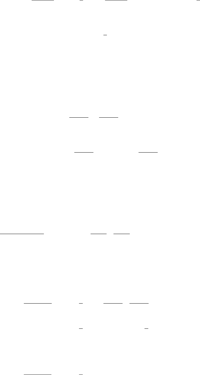
Chapter 7
Taking now the inverse Laplace transform, we obtain
y(t) = L
−1
s
s
2
+ 3
2
(t) +
1
3
L
−1
3
s
2
+ 3
2
G(s)
(t) = cos 3t +
1
3
sin(3t) ∗ g(t) .
Thus,
y(t) = cos 3t +
1
3
t
Z
0
sin [3(t − v)] g(v) dv.
4. Let Y (s) := L{y}(s), G(s) := L{g}(s). Taking the Laplace transform of both sides of
the given differential equation and using the linear property of the Laplace transform,
we obtain
s
2
Y (s) − 1
+ Y (s) = G(s) ⇒
s
2
+ 1
Y (s) = 1 + G(s)
⇒ Y (s) =
1
s
2
+ 1
+
G(s)
s
2
+ 1
.
Taking now the inverse Laplace transform, we obtain
y(t) = L
−1
1
s
2
+ 1
(t) + L
−1
1
s
2
+ 1
G(s)
(t)
= sin t + sin t ∗ g(t) = sin t +
t
Z
0
sin(t − v)g(v) dv .
6. From Table 7.1, Section 7.2, L
−1
{1/(s − a)}(t) = e
at
. Therefore, using the linearity of
the inverse Laplace transform and the convolution theorem, we have
L
−1
1
(s + 1)(s + 2)
(t) = L
−1
1
s + 1
·
1
s + 2
(t) = e
−t
∗ e
−2t
=
t
Z
0
e
−(t−v)
e
−2v
dve
−t
t
Z
0
e
−v
dv = e
−t
1 − e
−t
= e
−t
− e
−2t
.
8. Since 1/(s
2
+ 4)
2
= (1/4) [2/ (s
2
+ 2
2
)] · [2/ (s
2
+ 2
2
)], the convolution theorem tells us
L
−1
1
(s
2
+ 4)
2
(t) =
1
4
L
−1
2
s
2
+ 4
·
2
s
2
+ 4
(t)
=
1
4
sin(2t) ∗ sin(2t) =
1
4
t
Z
0
sin [2(t − v)] sin(2v) dv.
Using the identity sin α sin β = [cos(α − β) − cos(α + β)]/2, we get
L
−1
1
(s
2
+ 4)
2
(t) =
1
8
t
Z
0
[cos(2t − 4v) − cos 2t] dv
240

Exercises 7.7
=
1
8
sin(4v − 2t)
4
− v cos 2t
t
0
=
sin 2t
16
−
t cos 2t
8
.
10. We have
L
−1
1
s
3
(s
2
+ 1)
= L
−1
1
s
3
∗ L
−1
1
s
2
+ 1
=
t
2
2
∗ sin t =
1
2
t
Z
0
(t − v)
2
sin v dv
=
1
2
−(v − t)
2
cos v
t
0
+ 2
t
Z
0
(v − t) cos v dv
=
1
2
t
2
+ 2(v − t) sin v
t
0
−2
t
Z
0
sin v dv
=
t
2
2
+ cos t − 1 .
12. By the linearity of the inverse Laplace transform,
L
−1
s + 1
(s
2
+ 1)
2
(t) = L
−1
s
(s
2
+ 1)
2
(t) + L
−1
1
(s
2
+ 1)
2
(t) .
The second term can be evaluated similarly to that in Problem 8. (See also Example 2.)
L
−1
1
(s
2
+ 1)
2
(t) =
sin t − t cos t
2
. (7.23)
For the first term, we notice that s/(s
2
+ 1)
2
= [s/(s
2
+ 1)] · [1/(s
2
+ 1)] and apply the
convolution theorem.
L
−1
s
(s
2
+ 1)
2
(t) = L
−1
s
s
2
+ 1
·
1
s
2
+ 1
(t) = cos t ∗sin t =
t
Z
0
cos(t − v) sin v dv.
Using the identity sin α cos β = [sin(α + β) + sin(α −β)]/2, we get
L
−1
s
(s
2
+ 1)
2
(t) =
1
2
t
Z
0
[sin t + sin(t − 2v)] dv
=
1
2
v sin t +
cos(t − 2v)
2
v=t
v=0
=
t sin t
2
. (7.24)
Combining (7.23) and (7.24) yields
L
−1
s + 1
(s
2
+ 1)
2
(t) =
t sin t
2
+
sin t − t cos t
2
=
t sin t + sin t − t cos t
2
.
241

Chapter 7
14. Note that f(t) = e
t
∗ sin t. Hence, by formula (8) of the text,
L{f(t)}(s) = L
e
t
(s) · L{sin t}(s) =
1
s − 1
·
1
s
2
+ 1
=
1
(s − 1) (s
2
+ 1)
.
16. Note that
t
Z
0
e
t−v
y(v) dv = e
t
∗ y(t).
Let Y (s) := L{y}(s). Taking the Laplace transform of the original equation and using
Theorem 11, we obtain
Y (s) + L
e
t
∗ y(t)
(s) = Y (s) +
1
s − 1
Y (s) = L{sin t}(s) =
1
s
2
+ 1
⇒
1 +
1
s − 1
Y (s) =
1
s
2
+ 1
⇒ Y (s) =
s − 1
s (s
2
+ 1)
=
s
s
2
+ 1
+
1
s
2
+ 1
−
1
s
⇒ y(t) = L
−1
s
s
2
+ 1
+
1
s
2
+ 1
−
1
s
(t) = cos t + sin t −1 .
18. We use the convolution Theorem 11 to find the Laplace transform of the integral term.
L
t
Z
0
(t − v)y(v) dv
(s) = L{t ∗y(t)}(s) = L{t}(s)L{y(t)}(s) =
Y (s)
s
2
, (7.25)
where Y (s) denotes the Laplace transform of y(t). Thus taking the Laplace transform
of both sides of the given equation yields
Y (s) +
Y (s)
s
2
=
2
s
3
⇒ Y (s) =
2
s (s
2
+ 1)
= 2
1
s
−
s
s
2
+ 1
⇒ y(t) = L
−1
2
1
s
−
s
s
2
+ 1
(t) = 2 (1 −cos t) .
20. The Laplace transform of the integral term is found in Problem 18 (see (7.25)). Since
L{y
0
(t)}(s) = sY (s) − y(0) = sY (s) ,
taking the Laplace transform of both sides of the given equation yields
sY (s) +
Y (s)
s
2
=
s
3
+ 1
s
2
Y (s) = L{t}(s) =
1
s
2
⇒ Y (s) =
1
s
3
+ 1
=
1
(s + 1)(s
2
+ s + 1)
242

Exercises 7.7
=
1
3
1
s + 1
−
1
3
s − (1/2)
[s − (1/2)]
2
+
√
3/2
2
+
1
√
3
√
3/2
[s − (1/2)]
2
+
√
3/2
2
.
Therefore,
y(t) = L
−1
(
1
3
1
s + 1
−
1
3
s − (1/2)
[s − (1/2)]
2
+
√
3/2
2
+
1
√
3
√
3/2
[s − (1/2)]
2
+
√
3/2
2
)
(t)
=
1
3
e
−t
−
1
3
e
t/2
cos
√
3 t
2
!
+
1
√
3
e
t/2
sin
√
3 t
2
!
.
22. We rewrite the given integro-differential equation in the form
y
0
(t) − 2e
t
∗ y(t) = t
and take the Laplace transform of both sides using Theorem 11.
[sY (s) − y(0)] −
2
s − 1
Y (s) =
s −
2
s − 1
Y (s) − 2 =
1
s
2
⇒ Y (s) =
(2s
2
+ 1) (s − 1)
s
2
(s + 1)(s − 2)
=
1
2
1
s
2
−
3
4
1
s
+ (2)
1
s + 1
+
3
4
1
s − 2
,
where Y (s) = L{y}(s). Thus, taking the inverse Laplace transform yields
y(t) = L
−1
1
2
1
s
2
−
3
4
1
s
+ (2)
1
s + 1
+
3
4
1
s − 2
(t)
=
t
2
−
3
4
+ 2e
−t
+
3e
2t
4
.
24. Taking the Laplace transform of the differential equation, and assuming zero initial
conditions, we obtain
s
2
Y (s) − 9Y (s) =
s
2
− 9
Y (s) = G(s),
where Y = L{y}, G = L{g}. Thus, the transfer function
H(s) =
Y (s)
G(s)
=
1
s
2
− 9
.
The impulse response function is then
h(t) = L
−1
{H(s)}(t) = L
−1
1
s
2
− 9
(t)
= L
−1
1
6
1
s − 3
−
1
s + 3
(t) =
e
3t
− e
−3t
6
=
sinh 3t
3
.
243

Chapter 7
Next, we find the solution y
k
(t) to the corresponding homogeneous equation that satisfies
the initial conditions. Since the characteristic equation, r
2
− 9 = 0, has roots r = ±3,
we have
y
k
(t) = C
1
e
3t
+ C
2
e
−3t
⇒
y
k
(0) = C
1
+ C
2
= 2
y
0
k
(0) = 3C
1
− 3C
2
= 0
⇒ C
1
= C
2
= 1.
Therefore, y
k
(t) = e
3t
+ e
−3t
= 2 cosh 3t and
y(t) = (h ∗ g)(t) + y
k
(t) =
1
3
Z
t
0
sinh[3(t − v)]g(v) dv + 2 cosh 3t .
26. Taking the Laplace transform of both sides of the given equation and assuming zero
initial conditions, we get
L{y
00
+ 2y
0
− 15y}(s) = L{g(t)}(s) ⇒ s
2
Y (s) + 2sY (s) − 15Y (s) = G(s).
Thus,
H(s) =
Y (s)
G(s)
=
1
s
2
+ 2s − 15
=
1
(s − 3)(s + 5)
is the transfer function. The impulse response function h(t) is then given by
h(t) = L
−1
1
(s − 3)(s + 5)
(t) = e
3t
∗ e
−5t
=
t
Z
0
e
3(t−v)
e
−5v
dv = e
3t
−
e
−8v
8
t
0
!
=
e
3t
− e
−5t
8
.
To solve the given initial value problem, we use Theorem 12. To this end, we need the
solution y
k
(t) to the corresponding initial value problem for the homogeneous equation.
That is,
y
00
+ 2y
0
− 15y = 0, y(0) = 0, y
0
(0) = 8 .
Applying the Laplace transform yields
s
2
Y
k
(s) − 8
+ 2 [sY
k
(s)] − 15Y
k
(s) = 0
⇒ Y
k
(s) =
8
s
2
+ 2s − 15
=
8
(s − 3)(s + 5)
=
1
s − 3
−
1
s + 5
⇒ y
k
(t) = L
−1
1
s − 3
−
1
s + 5
(t) = e
3t
− e
−5t
.
So,
y(t) = (h ∗ g)(t) + y
k
(t) =
1
8
t
Z
0
e
3(t−v)
− e
−5(t−v)
g(v) dv + e
3t
− e
−5t
.
244

Exercises 7.7
28. Taking the Laplace transform and assuming zero initial conditions, we find the transfer
function H(s).
s
2
Y (s) − 4sY (s) + 5Y (s) = G(s) ⇒ H(s) =
Y (s)
G(s)
=
1
s
2
− 4s + 5
=
1
(s − 2)
2
+ 1
.
Therefore, the impulse response function is
h(t) = L
−1
{H(s)}(t) = L
−1
1
(s − 2)
2
+ 1
(t) = e
2t
sin t .
Next, we find the solution y
k
(t) to the corresp onding initial value problem for the ho-
mogeneous equation,
y
00
− 4y
0
+ 5y = 0, y(0) = 0, y
0
(0) = 1.
Since the associated equation, r
2
−4r + 5 = 0, has roots r = 2 ±i, a general solution to
the homogeneous equations is
y
h
(t) = e
2t
(C
1
cos t + C
2
sin t) .
We satisfy the initial conditions by solving
0 = y(0) = C
1
1 = y
0
(0) = 2C
1
+ C
2
⇒
C
1
= 0,
C
2
= 1.
Hence, y
k
(t) = e
2t
sin t and
y(t) = (h ∗ g)(t) + y
k
(t) =
t
Z
0
e
2(t−v)
[sin(t − v)] g(v) dv + e
2t
sin t
is the desired solution.
30. With given data, the initial value problem becomes
10I
00
(t) + 80I
0
(t) + 410I(t) = e(t) ⇒ I
00
(t) + 8I
0
(t) + 41I(t) =
e(t)
10
,
I(0) = 2, I
0
(0) = −8. Using formula (15) of the text, we find the transfer function
H(s) =
1
s
2
+ 8s + 41
=
1
(s + 4)
2
+ 5
2
.
Therefore,
h(t) = L
−1
1
(s + 4)
2
+ 5
2
(t) =
1
5
e
−4t
sin 5t .
245
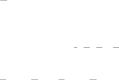
Chapter 7
Next, we consider the initial value problem
I
00
(t) + 8I
0
(t) + 41I(t) = 0, I(0) = 2, I
0
(0) = −8
for the corresponding homogeneous equation. Its characteristic equation, r
2
+8r+41 = 0,
has roots r = −4 ±5i, which give a general solution
I
h
(t) = e
−4t
(C
1
cos 5t + C
2
sin 5t) .
Next, we find constants C
1
and C
2
so that the solution satisfies the initial conditions.
Thus, we have
2 = I(0) = C
1
,
−8 = I
0
(0) = −4C
1
+ 5C
2
⇒
C
1
= 2 ,
C
2
= 0 ,
and so I
k
(t) = 2e
−4t
cos 5t. Finally,
I(t) = [h ∗ (e/10)] (t) + I
k
(t) =
1
50
t
Z
0
e
−4(t−v)
sin [5(t − v)] e(v) dv + 2e
−4t
cos 5t .
32. By the convolution theorem, we get
L
1 ∗ t ∗ t
2
(s) = L{1}(s)L{t}(s)L
t
2
(s) =
1
s
·
1
s
2
·
2
s
3
=
2
s
6
.
Therefore,
1 ∗ t ∗ t
2
= L
−1
2
s
6
(t) =
1
60
L
−1
5!
s
6
(t) =
t
5
60
.
34. Using the commutative property (4) of the convolution and Fubini’s theorem yields
(f ∗ g) ∗h = (g ∗ f) ∗h =
t
Z
0
(g ∗ f)(t − v)h(v) dv
=
t
Z
0
t−v
Z
0
g(t − v − u)f(u) du
h(v) dv =
t
Z
0
t−v
Z
0
g(t − v − u)f(u)h(v) du dv
=
t
Z
0
t−u
Z
0
g(t − u − v)h(v) dv
f(u) du =
t
Z
0
(g ∗ h)(t − u)f(u) du
= (g ∗ h) ∗ f = f ∗ (g ∗ h) .
246

Exercises 7.8
36. Let
G(t) :=
t
Z
0
v
Z
0
f(z) dz dv .
Clearly, G(0) = 0. By the fundamental theorem of calculus,
G
0
(t) =
t
Z
0
f(z) dz , G
0
(0) = 0 , G
00
(t) = f(t) .
Therefore, by Theorem 5 in Section 7.3, we get
F (s) = L{G
00
(t)}(s) = s
2
L{G(t)}(s) − sG(0) − G
0
(0) = s
2
L{G(t)}(s)
⇒ L{G(t)}(s) =
F (s)
s
2
⇒ G(t) = L
−1
F (s)
s
2
(t) .
We now apply Theorem 11 to conclude that
L
−1
1
s
2
F (s)
(t) =
L
−1
1
s
2
∗ L
−1
{F (s)}
(t) = t ∗f(t)
=
t
Z
0
(t − v)f(v) dv = t
t
Z
0
f(v) dv −
t
Z
0
vf(v) dv
EXERCISES 7.8: Impulses and the Dirac Delta Function
2. By equation (2) of the text,
∞
Z
−∞
e
3t
δ(t) dt = e
3t
t=0
= 1 .
4. By equation (3),
∞
Z
−∞
e
−2t
δ (t + 1) dt = e
−2t
t=−1
= e
2
.
6. Since δ(t) = 0 for t 6= 0,
1
Z
−1
(cos 2t)δ(t) dt =
∞
Z
−∞
(cos 2t)δ(t) dt = cos 2t|
t=0
= 1 .
8. Using the linearity of the Laplace transform and formula (6), we get
L{3δ(t − 1)}(s) = 3L{δ(t −1)}(s) = 3e
−s
.
247

Chapter 7
10. Since δ(t − 3) = 0 for t 6= 3,
L
t
3
δ(t − 3)
(s) :=
∞
Z
0
e
−st
t
3
δ(t − 3) dt =
∞
Z
−∞
e
−st
t
3
δ(t − 3) dt = e
−st
t
3
t=3
= 27e
−3s
by equation (3) of the text.
Another way to solve this problem is to use Theorem 6 in Section 7.3. This yields
L
t
3
δ(t − 3)
(s) = (−1)
3
d
3
ds
3
L{δ(t − 3)}(s) = −
d
3
(e
−3s
)
ds
3
= 27e
−3s
.
12. The translation property of the Laplace transform (Theorem 3, Section 7.3) yields
L
e
t
δ(t − 3)
(s) = L{δ(t − 3)}(s − 1) = e
−3(s−1)
= e
3(1−s)
.
14. Let Y (s) := L{y(t)}(s). Applying the Laplace transform to both sides of the given
equation, using Theorem 5 in Section 7.3 and the initial conditions, we find that
s
2
Y (s) − s − 1
+ 2 [sY (s) − 1] + 2Y (s) = L{δ(t −π)}(s) = e
−πs
.
Solving for Y (s) yields
Y (s) = e
−πs
1
s
2
+ 2s + 2
+
s + 3
s
2
+ 2s + 2
= e
−πs
1
(s + 1)
2
+ 1
+
s + 1
(s + 1)
2
+ 1
+2
1
(s + 1)
2
+ 1
Thus, by Theorem 8, Section 7.6 and Table 7.1 in Section 7.2,
y(t) =
e
−(t−π)
sin(t − π)
u(t − π) + e
−t
cos t + 2e
−t
sin t
= −e
π−t
(sin t) u(t − π) + e
−t
cos t + 2e
−t
sin t .
16. Let Y := L{y}. Taking the Laplace transform of y
00
− 2y
0
− 3y = 2δ(t − 1) − δ(t − 3)
and applying the initial conditions y(0) = 2, y
0
(0) = 2, we obtain
s
2
Y − 2s − 2
− 2 (sY −2) −3Y = L{2δ(t − 1) − δ(t −3)} = 2e
−s
− e
−3s
⇒ Y (s) =
2s − 2 + 2e
−s
− e
−3s
s
2
− 2s − 3
=
2s − 2 + e
−s
+ e
−3s
(s − 3)(s + 1)
=
1
s − 3
+
1
s + 1
+
e
−s
2
1
s − 3
−
1
s + 1
−
e
−3s
4
1
s − 3
−
1
s + 1
,
so that by Theorem 8, Section 7.6, we get
y(t) = e
3t
+ e
−t
+
1
2
e
3(t−1)
− e
−(t−1)
u(t − 1) −
1
4
e
3(t−3)
− e
−(t−3)
u(t − 3).
248

Exercises 7.8
18. Let Y := L{y}. Taking the Laplace transform of y
00
− y
0
− 2y = 3δ(t − 1) + e
t
and
applying the initial conditions y(0) = 0, y
0
(0) = 3, we obtain
s
2
Y − 3
− (sY ) − 2Y = L
3δ(t − 1) + e
t
=
1
s − 1
+ 3e
−s
⇒ Y (s) =
3s − 2
(s − 1) (s
2
− s − 2)
+ e
−s
3
s
2
− s − 2
=
3s − 2
(s − 1)(s − 2)(s + 1)
+ e
−s
3
(s − 2)(s + 1)
.
Taking the partial fractions decompositions yields
Y (s) =
4
3
1
s − 2
−
1
2
1
s − 1
−
5
6
1
s + 1
+ e
−s
1
s − 2
−
1
s + 1
so that from Table 7.1 in Section 7.2 and Theorem 8, Section 7.6, we get
y(t) =
4
3
e
2t
−
1
2
e
t
−
5
6
e
−t
+
e
2(t−1)
− e
−(t−1)
u(t − 1).
20. By the translation property of the Laplace transform,
L
e
−t
δ(t − 2)
(s) = L{δ(t − 2)}(s + 1) = e
−2(s+1)
.
Thus, the Laplace transform of the given equation yields
L{y
00
+ 5y
0
+ 6y} =
s
2
Y − 2s + 5
+ 5(sY −2) + 6Y = e
−2(s+1)
or, solving for Y := L{y(t)}(s),
Y =
2s + 5 + e
−2(s+1)
s
2
+ 5s + 6
2s + 5 + e
−2(s+1)
(s + 2)(s + 3)
=
1
s + 2
+
1
s + 3
+ e
−2
e
−2s
1
s + 2
−
1
s + 3
.
Applying now the inverse Laplace transform, we get
y(t) = e
−2t
+ e
−3t
+ e
−2
e
−2x
− e
−3x
x=t−2
u(t − 2)
= e
−2t
+ e
−3t
+ e
−2
e
−2(t−2)
− e
−3(t−2)
u(t − 2) .
22. We apply the Laplace transform to the given equation, solve the resulting equation for
Y = L{y}(s), and then use the inverse Laplace transform. This yields
L{y
00
}(s) + L{y}(s) = L
n
δ
t −
π
2
o
(s)
249

Chapter 7
⇒
s
2
Y (s) − 1
+ Y (s) = e
−πs/2
⇒ Y (s) =
1
s
2
+ 1
+ e
−πs/2
1
s
2
+ 1
⇒ y(t) = sin t +
h
sin
t −
π
2
i
u
t −
π
2
= sin t + (cos t)u
t −
π
2
.
The graph of the solution is shown in Fig. 7–M on page 266.
24. Similarly to Problem 22, we get
s
2
Y (s) − 1
+ Y (s) = e
−πs
− e
−2πs
⇒ Y (s) =
1
s
2
+ 1
+
e
−πs
− e
−2πs
1
s
2
+ 1
⇒ y(t) = sin t + [sin (t − π)] u (t −π) − [sin (t − 2π)] u (t −2π)
= (sin t) [1 − u(t − π) −u(t −2π)] .
The graph of the solution is shown in Fig. 7–N on page 266.
26. The Laplace transform of both sides of the given equation (with zero initial conditions)
yields
s
2
Y (s) − 6sY (s) + 13Y (s) = L{δ(t)}(s) = 1 .
Thus,
Y (s) =
1
s
2
− 6s + 13
=
1
(s − 3)
2
+ 2
2
=
1
2
2
(s − 3)
2
+ 2
2
.
Therefore, the impulse response function is
h(t) = L
−1
{Y (s)}(t) =
1
2
e
3t
sin 2t .
28. The Laplace transform of both sides of the given equation (with zero initial conditions)
yields
s
2
Y (s) − Y (s) = L{δ(t)}(s) = 1 .
Thus,
Y (s) =
1
s
2
− 1
=
1
(s − 1)(s + 1)
=
1
2
1
s − 1
−
1
s + 1
.
Therefore, the impulse response function is
h(t) = L
−1
{Y (s)}(t) =
1
2
e
t
− e
−t
= sinh t .
250

Exercises 7.8
30. Let Y := L{y(t)}. The Laplace transform of the left-hand side of the given equation
(with the imposed initial conditions) is (s
2
+ 1) Y (s) For the right-hand side, one has
L
(
∞
X
k=1
δ(t − 2kπ)
)
(s) =
∞
X
k=1
e
−2kπs
.
Hence,
Y (s) =
1
s
2
+ 1
∞
X
k=1
e
−2kπs
.
Taking the inverse Laplace transform in this equation yields the following sum y(t) of
the series of impulse response functions h
k
(t):
y(t) =
∞
X
k=1
h
k
(t) :=
∞
X
k=1
sin (t − 2kπ) u(t − 2kπ)
=
∞
X
k=1
(sin t) u(t − 2kπ) = (sin t)
∞
X
k=1
u(t − 2kπ) .
Evaluating y(t) at, say, t
n
= (π/2) + 2nπ for n = 1, 2, . . . we see that
y (t
n
) =
h
sin
π
2
+ 2nπ
i
∞
X
k=1
u (t − 2kπ) =
n
X
k=1
(1) = n → ∞
with t
n
→ ∞, meaning that the bridge will eventually collapse.
32. By taking the Laplace transform of
ay
00
+ by
0
+ cy = δ(t), y(0) = y
0
(0) = 0,
and solving for Y := L{y}, we find that the transfer function is given by
H(s) =
1
as
2
+ bs + c
.
We consider the following possibilities.
(i) If the roots of the polynomial as
2
+ bs + c are real and distinct, say r
1
, r
2
, then
H(s) =
1
a(s − r
1
)(s − r
2
)
=
1
a(r
1
− r
2
)
1
s − r
1
−
1
s − r
2
.
Thus,
h(t) = L
−1
{H(s)}(t) =
1
a (r
1
− r
2
)
e
r
1
t
− e
r
2
t
and, clearly, h(t) has zero limit as t → ∞ if and only if r
1
and r
2
are negative.
251
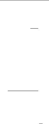
Chapter 7
(ii) If the roots of as
2
+ bs + c are complex, then they are α ± iβ, where α and β 6= 0
satisfy
H(s) =
1
a [(x − α)
2
+ β
2
]
so that
h(t) = L
−1
{H(s)}(t) =
1
aβ
e
αt
sin βt ,
and, again, it is clear that h(t) → 0 as t → ∞ if and only if the real part α of the
roots is negative.
(iii) Finally, if the characteristic equation has a double real root r
0
, then
H(s) =
1
a (r − r
0
)
2
,
implying that
h(t) = L
−1
{H(s)}(t) =
1
a
te
r
0
t
,
which, again, vanishes at infinity if and only if r
0
< 0.
34. Let a function f (t) be defined and n times continuously differentiable in a neighborhood
[−, ] of the origin. Since, for t 6= 0, δ(t) and all its derivatives equal zero, we can
(formally) consider the improper integral
R
∞
−∞
f(t)δ
(n)
(t)dt assuming that the integrand
vanishes outside of [−, ]. Then, applying integration by parts n times yields
∞
Z
−∞
f(t)δ
(n)
(t) dt =
Z
−
f(t)δ
(n)
(t) dt = f(t)δ
(n−1)
(t)
−
−
Z
−
f
0
(t)δ
(n−1)
(t) dt
= −
Z
−
f
0
(t)δ
(n−1)
(t) dt = ··· = (−1)
n
Z
−
f
(n)
(t)δ(t) dt
= (−1)
n
∞
Z
−∞
f
(n)
(t)δ(t) dt = (−1)
n
f
(n)
(0)
by equation (2) of the text.
EXERCISES 7.9: Solving Linear Systems with Laplace Transforms
2. Let X = L{x}, Y = L{y}. Applying the Laplace transform to both sides of the given
equations and using Theorem 4, Section 7.3, for evaluating Laplace transforms of the
252

Exercises 7.9
derivatives yields
sX(s) + 1 = X(s) −Y (s)
sY (s) = 2X(s) + 4Y (s)
⇒
(s − 1)X(s) + Y (s) = −1
−2X(s) + (s −4)Y (s) = 0 .
Solving this system for, say, Y (s), we obtain
Y (s) = −
2
s
2
− 5s + 6
= −
2
(s − 2)(s − 3)
=
2
s − 2
−
2
s − 3
.
Therefore,
y(t) = L
−1
2
s − 2
−
2
s − 3
(t) = 2e
2t
− 2e
3t
.
From the second equation in the given system we find that
x(t) =
1
2
(y
0
− 4y) =
1
2
4e
2t
− 6e
3t
− 4
2e
2t
− 2e
3t
= −2e
2t
+ e
3t
.
4. Let X = L{x}, Y = L{y}. Applying the Laplace transform to both sides of the given
equations and using Theorem 4, Section 7.3, for evaluating Laplace transforms of the
derivatives yields
sX(s) −3X(s) + 2Y (s) = 1/ (s
2
+ 1)
4X(s) −sY (s) − Y (s) = s/ (s
2
+ 1)
⇒
(s − 3)X(s) + 2Y (s) = 1/ (s
2
+ 1)
4X(s) −(s + 1)Y (s) = s/ (s
2
+ 1) .
Solving this system for X(s), we obtain
X(s) =
3s + 1
(s
2
+ 1) (s
2
− 2s + 5)
=
3s + 1
(s
2
+ 1) [(s − 1)
2
+ 2
2
]
.
The partial fractions decomposition for X(s) is
X(s) =
7
10
s
s
2
+ 1
−
1
10
1
s
2
+ 1
−
7
10
s − 1
(s − 1)
2
+ 2
2
+
2
5
2
(s − 1)
2
+ 2
2
.
Hence, the inverse Laplace transform gives us
x(t) =
7
10
cos t −
1
10
sin t −
7
10
e
t
cos 2t +
2
5
e
t
sin 2t .
From the first equation in the system,
y(t) =
sin t − x
0
(t) + 3x(t)
2
.
Substituting the solution x(t) and collecting similar terms yields
y(t) =
11
10
cos t +
7
10
sin t −
11
10
e
t
cos 2t −
3
5
e
t
sin 2t .
253

Chapter 7
6. Denote X = L{x}, Y = L{y}. The Laplace transform of the given equations yields
sX(s) −X(s) − Y (s) = 1/s
−X(s) + sY (s) + (5/2) − Y (s) = 0
⇒
(s − 1)X(s) −Y (s) = 1/s
−X(s) + (s −1)Y (s) = −(5/2) .
We multiply the first equation by (s − 1) and add to the second equation.
(s − 1)
2
− 1
X(s) =
s − 1
s
−
5
2
= −
3s + 2
2s
⇒ X(s) = −
3s + 2
2s [(s − 1)
2
− 1]
= −
1
2
3s + 2
s
2
(s + 2)
=
1
2s
2
+
1
s
−
1
s − 2
.
Taking the inverse Laplace transform we find
x(t) =
t
2
+ 1 − e
2t
.
From the first equation in the given system,
y(t) = x
0
(t) − x(t) − 1 = −
t
2
−
3
2
− e
2t
.
8. By taking the Laplace transform of both sides of these differential equations and using
the linearity of the Laplace transform, we obtain
L{D[x]}(s) + L{y}(s) = L{0}(s) = 0
4L{x}(s) + L{D[y]}(s) = L{3}(s) = 3/s
⇒
sX(s) −(7/4) + Y (s) = 0
4X(s) + sY (s) − 4 = 3/s
or, equivalently,
sX(s) + Y (s) = (7/4)
4X(s) + sY (s) = (4s + 3)/s ,
where X(s) and Y (s) are the Laplace transforms of x(t) and y(t), respectively. Solving
this system for X(s) yields
X(s) =
7s
2
− 16s − 12
4s (s
2
− 4)
=
3
4
1
s
+
3
2
1
s + 2
−
1
2
1
s − 2
.
The inverse Laplace transform leads now to
x(t) = L
−1
3
4
1
s
+
3
2
1
s + 2
−
1
2
1
s − 2
(t) =
3
4
+
3
2
e
−2t
−
1
2
e
2t
.
Differentiating x(t), we find y(t). (See the first equation in the given system.)
y(t) = −x
0
(t) = 3e
−2t
+ e
2t
.
254

Exercises 7.9
10. Denote X = L{x}, Y = L{y}. The Laplace transform of the given equations (for the
given initial conditions) yields
s
2
X(s) −s −1 + Y (s) = 1/s
X(s) + s
2
Y (s) − s + 1 = −1/s
⇒
s
2
X(s) + Y (s) = s + 1 + (1/s)
X(s) + s
2
Y (s) = s −1 − (1/s) .
If we multiply the first equation by s
2
and subtract the second equation from the result,
we get
s
4
− 1
X(s) = s
3
+ s
2
+ 1 +
1
s
=
s
4
+ s
3
+ s + 1
s
⇒ X(s) =
s
4
+ s
3
+ s + 1
s (s
4
− 1)
=
s
4
+ s
3
+ s + 1
s(s − 1)(s + 1) (s
2
+ 1)
,
which, using partial fractions, can be written as
X(s) =
s
s
2
+ 1
+
1
s − 1
−
1
s
.
Taking the inverse Laplace transform, we find that
x(t) = cos t + e
t
− 1 .
From the first equation in the given system,
y(t) = 1 − x
00
(t) = cos t −e
t
+ 1 .
12. Since
L{x
0
}(s) = sX(s) − x(0) = sX(s) ,
L{y
00
}(s) = s
2
Y (s) − sy(0) −y
0
(0) = s
2
Y (s) − s + 1 ,
applying the Laplace transform to the given equations yields
sX(s) + Y (s) = X(s)
2sX(s) + s
2
Y (s) − s + 1 = e
−3s
/s
⇒
(s − 1)X(s) + Y (s) = 0
2sX(s) + s
2
Y (s) = s −1 + e
−3s
/s .
Solving for X(s) yields
X(s) =
1 − s − e
−3s
s (s
2
− s − 2)
=
1 − s
s(s + 1)(s − 2)
− e
−3s
1
s
2
(s + 1)(s − 2)
= −
1
2s
+
(2/3)
s + 1
−
(1/6)
s − 2
− e
−3s
1
4s
−
1
2s
2
−
(1/3)
s + 1
+
(1/12)
s − 2
.
255

Chapter 7
Using linearity of the inverse Laplace transform and formula (6) in Section 7.6, we get
x(t) = −
1
2
+
2
3
e
−t
−
1
6
e
2t
−
1
4
−
x
2
−
1
3
e
−x
+
1
12
e
2x
x=t−3
u(t − 3)
= −
1
2
+
2e
−t
3
−
e
2t
6
−
1
4
−
t − 3
2
−
e
3−t
3
+
e
2t−6
12
u(t − 3) .
Since y = x −x
0
(see the first equation in the given system), we obtain
y(t) = −
1
2
+
4e
−t
3
+
e
2t
6
−
3
4
−
t − 3
2
−
2e
3−t
3
−
e
2t−6
12
u(t − 3) .
14. Since
L{x
00
}(s) = s
2
X(s) −sx(0) −x
0
(0) = s
2
X(s) −s ,
L{y
00
}(s) = s
2
Y (s) − sy(0) −y
0
(0) = s
2
Y (s) ,
applying the Laplace transform to the given equations yields
s
2
X(s) −s = Y (s) + e
−s
/s
s
2
Y (s) = X(s) + (1/s) − e
−s
/s
⇒
s
2
X(s) −Y (s) = s + (e
−s
/s)
−X(s) + s
2
Y (s) = (1/s) − (e
−3s
/s) .
Solving for X(s) yields
X(s) =
s
4
+ 1
s (s
4
− 1)
+
s
2
− 1
s (s
4
− 1)
e
−s
=
s
4
+ 1
s (s
4
− 1)
+
1
s (s
2
+ 1)
e
−s
= −
1
s
+
1
2
1
s + 1
+
1
2
1
s − 1
+
s
s
2
+ 1
+
1
s
−
s
s
2
+ 1
e
−s
.
Using linearity of the inverse Laplace transform and formula (6) in Section 7.6, we get
x(t) = −1 +
e
−t
2
+
e
t
2
+ cos t + [1 − cos(t − 1)] u(t − 1)
= cosh t + cos t − 1 + [1 − cos(t − 1)] u(t − 1) .
Since y = x
00
− u(t − 1) (see the first equation in the system), after some algebra we
obtain
y(t) = cosh t − cos t − [1 − cos(t − 1)] u(t − 1) .
16. First, note that the initial conditions are given at the point t = π. Thus, for the Laplace
transform method, we have to shift the argument to get zero initial point. Let us denote
w(t) := x(t + 1) and v(t) := y(t + π).
256

Exercises 7.9
The chain rule yields
w
0
(t) = x
0
(t + π)(t + π)
0
= x
0
(t + π), v
0
(t) = y
0
(t + π)(t + π)
0
= y
0
(t + π).
In the original system, we substitute t + π for t to get
w
0
(t) − 2w(t) + v
0
(t) = −[cos(t + π) + 4 sin(t + π)] = cos t + 4 sin t
2w(t) + v
0
(t) + v(t) = sin(t + π) + 3 cos(t + π) = −sin t −3 cos t
with initial conditions w(0) = x(π) = 0, v(0) = y(π) = 3. Taking the Laplace transform
and using Theorem 4, Section 7.3, we obtain the system
sW (s) − 2W (s) + sV (s) − 3 =
s + 4
s
2
+ 1
2W (s) + sV (s) −3 + V (s) =
−3s − 1
s
2
+ 1
or, after collecting similar terms,
(s − 2)W (s) + sV (s) =
3s
2
+ s + 7
s
2
+ 1
2W (s) + (s + 1)V (s) =
3s
2
− 3s + 2
s
2
+ 1
.
Solving this system for V (s) yields
V (s) =
3s
3
− 15s
2
+ 6s − 18
(s
2
+ 1) (s
2
− 3s − 2)
=
3s
3
− 15s
2
+ 6s − 18
(s
2
+ 1)
s − (3 +
√
17)/2
s − (3 −
√
17)/2
= −
s
s
2
+ 1
+
2
√
17 − 12
√
17
!
1
s − (3 +
√
17)/2
+
2
√
17 + 12
√
17
!
1
s − (3 −
√
17)/2
.
Therefore, taking the inverse Laplace transform, we obtain
v(t) = −cos t +
2
√
17 − 12
√
17
!
e
(3+
√
17)t/2
+
2
√
17 + 12
√
17
!
e
(3−
√
17)t/2
.
Shifting the argument back gives
y(t) = v(t − π) = cos t +
2
√
17 − 12
√
17
!
e
(3+
√
17)(t−π)/2
+
2
√
17 + 12
√
17
!
e
(3−
√
17)(t−π)/2
.
We can now find x(t) by substituting y(t) into the second equation of the original system.
x(t) =
sin t + 3 cos t − y
0
(t) − y(t)
2
= cos t + sin t +
√
17 + 13
2
√
17
!
e
(3+
√
17)(t−π)/2
+
√
17 − 13
2
√
17
!
e
(3−
√
17)(t−π)/2
.
257

Chapter 7
18. We first take the Laplace transform of both sides of all three of these equations and use
the initial conditions to obtain a system of equations for the Laplace transforms of the
solution functions.
sX(s) −2Y (s) = 0
sX(s) −[sZ(s) + 2] = 0
X(s) + sY (s) − Z(s) = 3/s
⇒
sX(s) −2Y (s) = 0
sX(s) −sZ(s) = 2
X(s) + sY (s) − Z(s) = 3/s .
Solving this system yields
X(s) =
2
s
3
, Y (s) =
1
s
2
, Z(s) =
2
s
3
−
2
s
.
Taking the inverse Laplace transforms, we get
x(t) = L
−1
{X(s)}(t) = t
2
, y(t) = L
−1
{Y (s)}(t) = t , z(t) = L
−1
{Z(s)}(t) = t
2
− 2 .
20. Taking the Laplace transforms of the given equations yields
s
2
X(s) −3s + sY (s) − y(0) = 2/s
4X(s) + sY (s) − y(0) = 6/s
⇒
s
2
X(s) + sY (s) − y(0) = 2/s + 3s
4X(s) + sY (s) − y(0) = 6/s .
Subtracting the second equation from the first one, we get
s
2
− 4
X(s) =
3s
2
− 4
s
⇒ X(s) =
3s
2
− 4
s (s
2
− 4)
=
1
s
+
1
s − 2
+
1
s + 2
.
We now take the inverse Laplace transform and conclude that
x(t) = L
−1
{X(s)}(t) = 1 + e
2t
+ e
−2t
= 1 + 2 cosh 2t .
From the second equation in the original system,
y
0
(t) = 6 −4x(t) = 2 − 8 cosh 2t .
Integrating y
0
(s) from s = 1 (due to the initial condition) to s = t we obtain
y(t) =
t
Z
1
(2 − 8 cosh 2s)ds + 4 = (2s −4 sinh 2s)
t
1
+4 = 2t −4 sinh 2t + 2 + 4 sinh 2 .
22. For the mass m
1
there is only one force acting on it, that is, the force due to the spring
with the spring constant k
1
; so, it equals to −k
1
(x − y). Hence, we get
m
1
x
00
= −k
1
(x − y).
258

Exercises 7.9
For the mass m
2
, there are two forces: the force due to the spring with the spring
constant k
2
, which is −k
2
y; and the force due to the spring with the spring constant k
1
,
which is k
1
(y − x). Thus, we get
m
2
y
00
= k
1
(x − y) − k
2
y.
Therefore, the system governing the motion is
m
1
x
00
= k
1
(y − x)
m
2
y
00
= −k
1
(y − x) − k
2
y .
With m
1
= 1, m
2
= 2, k
1
= 4, and k
2
= 10/3 the system becomes
x
00
+ 4x − 4y = 0
−4x + 2y
00
+ (22/3) y = 0
(7.26)
with initial conditions
x(0) = −1, x
0
(0) = 0, y(0) = 0, y
0
(0) = 0 .
The Laplace transform of this system yields
[s
2
X(s) + s] + 4X(s) − 4Y (s) = 0
−4X(s) + 2 [s
2
Y (s)] + (22/3)Y (s) = 0
⇒
(s
2
+ 4) X(s) −4Y (s) = −s
−2X(s) + (s
2
+ (11/3)) Y (s) = 0 .
Multiplying the first equation by 2, the second equation – by s
2
+ 4 and adding the
results together, we obtain
s
2
+
11
3
s
2
+ 4
− 8
Y (s) = −2s
⇒ Y (s) = −
6s
3s
4
+ 23s
2
+ 20
= −
6
17
s
s
2
+ 1
+
6
17
s
s
2
+ (20/3)
.
Therefore,
y(t) = L
−1
{Y (s)}(t) = −
6
17
cos t +
6
17
cos
r
20
3
t
!
.
From the second equation in (7.26), we have
x(t) =
y
00
(t) + (11/3)y(t)
2
= −
8
17
cos t −
9
17
cos
r
20
3
t
!
.
259

Chapter 7
24. Recall that Kirchhoff’s voltage law says that, in an electrical circuit consisting of an
inductor of L (H), a resistor of R (Ω), a capacitor of C (F), and a voltage source of
E (V),
E
L
+ E
R
+ E
C
= E, (7.27)
where E
L
, E
R
, and E
C
denote the voltage drops across the inductor, resistor, and ca-
pacitor, respectively. These voltage grops are given by
E
L
= L
dI
dt
, E
R
:= RI, E
C
:=
q
C
, (7.28)
where I denotes the current passing through the correspondent element.
Also, Kirchhoff’s current law states that the algebraic sum of currents passing through
any point in an electrical network is zero.
The electrical network shown in Figure 7.29 consists of three closed circuits: loop 1
through the battery B = 50 (V), L
1
= 0.005 (H) inductor, and R
1
= 10 (Ω) resistor;
loop 2 through the resistor R
1
, the inductor L
2
= 0.01 (H), and the resistor R
2
= 20 (Ω);
loop 3 through the battery B, the inductors L
1
and L
2
, and the resistor R
2
. We apply
Kirchhoff’s voltage law (7.27) to two of these loops, say, the lo op 1 and the loop 2 (since
the equation obtained from Kirchhoff’s voltage law for the loop 3 is a linear combination
of the other two), and Kirchhoff’s current law to one of the junction points, say, the upper
one. Thus, choosing the clockwise direction in the loops and using formulas (7.28), we
obtain
Loop 1:
E
L
1
+ E
R
1
= E ⇒ 0.005I
0
1
+ 10I
2
= 50;
Loop 2:
E
R
1
+ E
L
2
+ E
R
2
= 0 ⇒ 0.01I
0
3
+ 10 (−I
2
+ 2I
3
) = 0
with the negative sign at I
2
due to the opposite direction of the current in this loop
versus to that in Loop 1;
Upper junction point:
I
1
− I
2
− I
3
= 0 .
260

Exercises 7.9
Therefore, we have the following system for the currents I
1
, I
2
, and I
3
:
0.005I
0
1
+ 10I
2
= 50
0.01I
0
3
+ 10 (−I
2
+ 2I
3
) = 0
I
1
− I
2
− I
3
= 0
(7.29)
with initial conditions I
1
(0) = I
2
(0) = I
3
(0) = 0.
Let I
1
(s) := L{I
1
}(s), I
2
(s) := L{I
2
}(s), and I
3
(s) := L{I
3
}(s). Using the initial
conditions, we conclude that
L{I
0
1
}(s) = sI
1
(s) − I
1
(0) = sI
1
(s),
L{I
0
3
}(s) = sI
3
(s) − I
3
(0) = sI
3
(s).
Using these equations and taking the Laplace transform of the equations in (7.29), we
come up with
0.005sI
1
(s) + 10I
2
(s) =
50
s
−10I
2
(s) + (0.01s + 20) I
3
(s) = 0
I
1
(s) − I
2
(s) − I
3
(s) = 0 .
Expressing I
2
(s) = I
1
(s) − I
3
(s) from the last equation and substituting this into the
the first two equations, we get
(0.005s + 10) I
1
(s) − 10I
3
(s) =
50
s
−10I
1
(s) + (0.01s + 30) I
3
(s) = 0 .
Solving this system for, say, I
3
(s), we obtain
I
3
(s) =
10
7
s (s
2
+ 5 · 10
3
s + 4 · 10
6
)
=
5
2s
−
10
3(s + 1000)
+
5
6(s + 4000)
.
The inverse Laplace transform then yields
I
3
(t) =
5
2
−
10
3
e
−1000t
+
5
6
e
−4000t
.
From the second equation in (7.29), we find
I
2
(t) =
0.01I
0
3
(t) + 20I
3
(t)
10
= 5 −
10
3
e
−1000t
−
5
3
e
−4000t
.
Finally, the last equation in (7.29) yields
I
1
(t) = I
2
(t) + I
3
(t) =
15
2
−
20
3
e
−1000t
−
5
6
e
−4000t
.
261

Chapter 7
REVIEW PROBLEMS
2.
1 − e
−5(s+1)
s + 1
−
e
−5s
s
4.
4
(s − 3)
2
+ 16
6.
7(s − 2)
(s − 2)
2
+ 9
−
70
(s − 7)
2
+ 25
8. 2s
−3
+ 6s
−2
− (s − 2)
−1
− 6(s − 1)
−1
10.
s
s
2
+ 1
+
e
−πs/2
(1 + s
2
)(1 − e
−πs
)
12. 2e
2t
cos(
√
2 t) +
3
√
2
e
2t
sin(
√
2 t)
14. e
−t
− 3e
−3t
+ 3e
2t
16.
sin 3t − 3t cos 3t
54
18. f (t) =
∞
X
n=0
(−1)
n
t
2n
n!
; F (s) =
∞
X
n=0
(−1)
n
(2n)!
n!
1
s
2n+1
20. (t − 3)e
−3t
22.
10
13
e
2t
−
23
13
cos 3t +
15
13
sin 3t
24. 6e
t
+ 4te
t
+ t
2
e
t
+ 2te
2t
− 6e
2t
26.
1 + Ct
3
e
−t
, where C is an arbitrary constant
28.
3
2
√
7
e
−t/2
sin
√
7 t
2
!
−
1
2
e
−t/2
cos
√
7 t
2
!
−
1
2
30.
1
2
n
sin 2t +
h
sin 2
t −
π
2
i
u
t −
π
2
o
32. x = −
1
2
+
1
6
e
2t
+
4
3
e
−t
+
−
1
4
+
1
2
(t − 3) −
1
12
e
2t−6
−
2
3
e
−t+3
u(t −3)
y = −
1
2
−
1
6
e
2t
+
2
3
e
−t
+
1
4
+
1
2
(t − 3) +
1
12
e
2t−6
−
1
3
e
−t+3
u(t − 3)
262
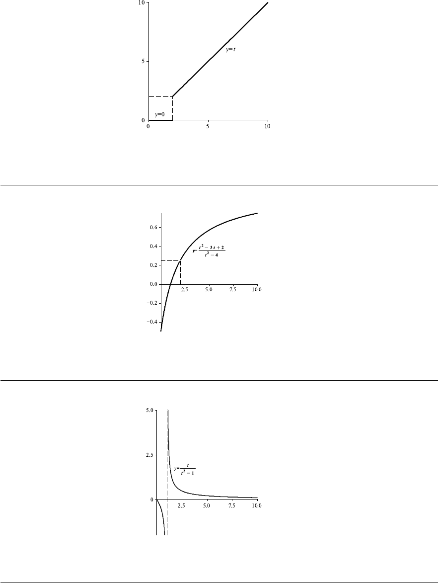
Figures
FIGURES
Figure 7–A: The graph of f(t) in Problem 22.
Figure 7–B: The graph of f(t) in Problem 24.
Figure 7–C: The graph of f(t) in Problem 26.
263
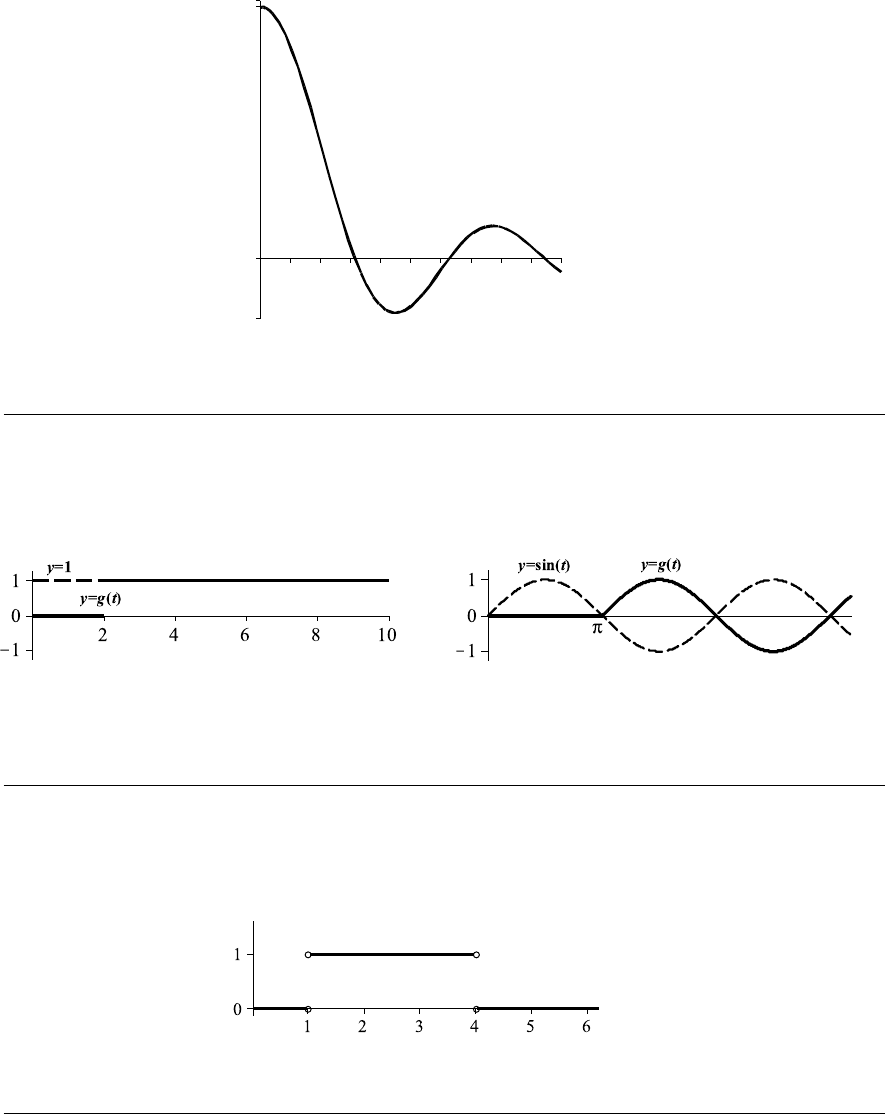
Chapter 7
105
0
1
0
y=
sin t/t, t 6= 0
1, t = 0
Figure 7–D: The graph of f(t) in Problem 28.
(a) (b)
Figure 7–E: Graphs of functions f(t) and g(t) in Problems 32 and 34.
Figure 7–F: The graph of the function in Problem 2.
264
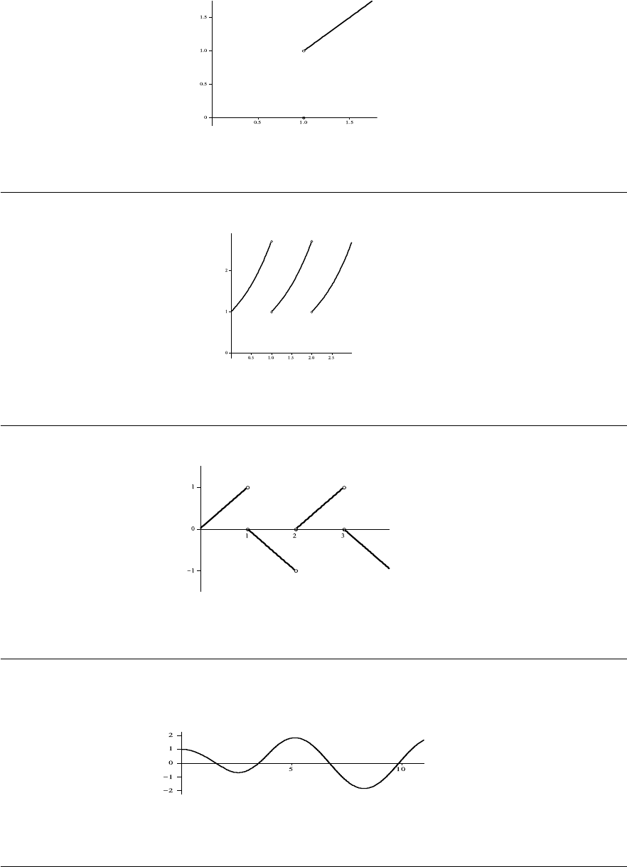
Figures
Figure 7–G: The graph of the function in Problem 4.
Figure 7–H: The graph of f(t) in Problem 22.
Figure 7–I: The graph of f(t) in Problem 24.
Figure 7–J: The graph of w(t) in Problem 30.
265
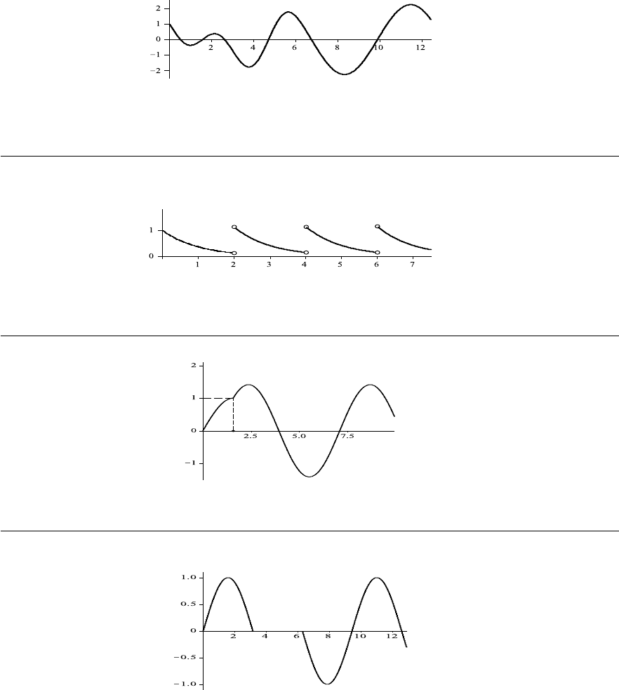
Chapter 7
Figure 7–K: The graph of y(t) in Problem 32.
Figure 7–L: The graph of g(t) in Problem 42.
Figure 7–M: The graph of y(t) in Problem 22.
Figure 7–N: The graph of y(t) in Problem 24.
266

CHAPTER 8: Series Solutions of Differential
Equations
EXERCISES 8.1: Introduction: The Taylor Polynomial Approximation
2. 2 + 4x + 8x
2
+ ···
4.
1
2
x
2
+
1
6
x
3
−
1
20
x
5
+ ···
6. x −
1
6
x
3
+
1
120
x
5
+ ···
8. 1 −
sin 1
2
x
2
+
(cos 1)(sin 1)
24
x
4
+ ···
10. (a) p
3
(x) =
1
2
+
x
4
+
x
2
8
+
x
3
16
(b) ε
3
=
1
4!
24
(2 − ξ)
5
1
2
4
≤
1
(3/2)
5
1
2
4
=
2
3
5
≈ 0.00823
(c)
2
3
− p
3
1
2
=
1
384
≈ 0.00260
(d) See Fig. 8–A on page 276
12. The differential equation implies that the functions y(x), y
0
(x), and y
00
(x) exist and
continuous. Furthermore, y
000
(x) can be obtained by differentiating the other terms:
y
000
= −py
00
− p
0
y
0
− qy
0
− q
0
y + g
0
. Since p, q, and g have derivatives of all orders,
subsequent differentiations display the fact that, in turn, y
000
, y
(4)
, y
(5)
, etc. all exist.
14. (a) t +
t
2
2
−
t
3
6
+ ···
(b) For r = 1, y(t) = 1 − (1/2)t
2
− 4t
4
+ ···;
For r = −1, y(t) = 1 + (1/2)t
2
− (49/12)t
4
+ ···
(c) For small t in part (b), the hard spring recoils but the soft spring extends.
16. 1 −
t
2
2
+
t
4
4
+ ···
267

Chapter 8
EXERCISES 8.2: Power Series and Analytic Functions
2. (−∞, ∞)
4. [2, 4]
6. (−3, −1)
8. (a)
−
1
2
,
1
2
(b)
−
1
2
,
1
2
(c) (−∞, ∞)
(d) (−∞, ∞)
(e) (−∞, ∞)
(f)
−
1
√
2
,
1
√
2
10.
∞
X
n=0
2
n+3
(n + 3)!
+
(n + 2)
2
2
n+1
(x − 1)
n
12. x −
2
3
x
3
+
2
15
x
5
+ ···
14. 1
16. 1 −
1
2
x +
1
4
x
2
−
1
24
x
3
+ ···
18.
∞
X
k=0
(−1)
k
(2k)!
x
2k
= cos x
20.
∞
X
n=2
n(n − 1)a
n
x
n−2
22.
∞
X
k=0
(−1)
k
(2k + 1)(2k + 1)!
x
2k+1
= x −
x
3
18
+
x
5
600
− ···
24.
∞
X
k=4
(k − 2)(k − 3)a
k−2
x
k
26.
∞
X
k=4
a
k−3
k
x
k
268

Exercises 8.3
30.
∞
X
n=0
(−1)
n
(x − 1)
n
32.
∞
X
n=1
(−1)
n+1
n
x
n
34. 1 +
1
2
(x − 1) −
1
8
(x − 1)
2
+
1
16
(x − 1)
3
−
5
128
(x − 1)
4
+ ···
36. (a) Always true
(b) Sometimes false
(c) Always true
(d) Always true
38.
∞
X
n=0
(−1)
n
n + 1
x
2n+2
= x
2
−
x
4
2
+
x
6
3
− ···
EXERCISES 8.3: Power Series Solutions to Linear Differential Equations
2. 0
4. −1, 0
6. −1
8. No singular points
10. x ≤ 1 and x = 2
12. y = a
0
1 + x +
x
2
2!
+
x
3
3!
+ ···
= a
0
∞
X
n=0
x
n
n!
= a
0
e
x
14. a
0
1 −
x
2
2
+ ···
+ a
1
x −
x
3
6
+ ···
16. a
0
1 −
x
2
2
−
x
3
3
+ ···
+ a
1
x + x
2
+
x
3
2
+ ···
= a
0
e
x
+ (a
1
− a
0
) xe
x
18. a
0
1 +
x
2
6
+ ···
+ a
1
x +
x
3
27
+ ···
20. a
0
∞
X
k=0
(−1)
k
x
2k
(2k)!
+ a
1
∞
X
k=0
(−1)
k
x
2k+1
(2k + 1)!
= a
0
cos x + a
1
sin x
269

Chapter 8
22. a
3k+2
= 0, k = 0, 1, . . .
a
0
1 +
∞
X
k=1
(−1)
k
1 · 4 ···(3k − 5)(3k − 2)
(3k)!
x
3k
!
+a
1
x +
∞
X
k=1
(−1)
k
2 · 5 ···(3k − 4)(3k − 1)
(3k + 1)!
x
3k+1
!
24. a
0
"
1 −
x
2
2
+
x
4
24
+
∞
X
k=3
(−1)
k
(2k − 3)
2
(2k − 5)
2
···3
2
(2k)!
x
2k
#
+ a
1
x
26. x +
x
2
2
+
x
3
2
+
x
4
3
+ ···
28. −1 −
x
2
2
−
x
3
3
−
x
4
8
+ ···
30. −1 + x +
5x
2
2
−
x
3
6
32. (a) If a
1
= 0, then y(x) is an even function;
(d) a
0
= 0, a
1
> 0
36. 3 −
9t
2
2
+ t
3
+ t
4
+ ···
EXERCISES 8.4: Equations with Analytic Coefficients
2. Infinite
4. 2
6. 1
8. a
0
1 − 2(x + 1) + 3(x + 1)
2
−
10
3
(x + 1)
3
+ ···
10. a
0
1 −
1
4
(x − 2)
2
−
1
24
(x − 2)
3
+ ···
+ a
1
(x − 2) +
1
4
(x − 2)
2
−
1
12
(x − 2)
3
+ ···
12. a
0
1 +
1
2
(x + 1)
2
+
2
3
(x + 1)
3
+ ···
+ a
1
(x + 1) + 2(x + 1)
2
+
7
3
(x + 1)
3
+ ···
14. 1 + x + x
2
+
5x
3
6
+ ···
16. −t +
t
3
3
+
t
4
12
+
t
5
24
+ ···
270

Exercises 8.6
18. 1 +
x −
π
2
+
1
2
x −
π
2
2
−
1
24
x −
π
2
4
+ ···
22. a
0
1 −
x
2
2
+ ···
+
x +
x
2
2
−
x
3
6
+ ···
24. a
0
1 −
3x
2
2
+ ···
+ a
1
x −
x
3
6
+ ···
+
2
3
− x
2
26. a
0
1 − x
2
+ a
1
x −
x
3
6
+ ···
+
x
2
2
+ ···
28. a
0
1 +
x
3
6
+ ···
+ a
1
(x + ···) +
x
2
2
+ ···
30. 1 −
t
2
2
+
t
3
2
−
t
4
4
+ ···
EXERCISES 8.5: Cauchy-Euler (Equidimensional) Equations Revisited
2. c
1
x
−5/2
+ c
2
x
−3
4. c
1
x
−
(
1+
√
13
)
/2
+ c
2
x
−
(
1−
√
13
)
/2
6. c
1
x cos
√
3 ln x
+ c
2
x sin
√
3 ln x
8. c
1
+ c
2
x
−1/2
cos
√
5
2
ln x
!
+ c
3
x
−1/2
sin
√
5
2
ln x
!
10. c
1
x
−2
+ c
2
x
−2
ln x + c
3
x
−2
(ln x)
2
12. c
1
(x + 2)
1/2
cos [ln(x + 2)] + c
2
(x + 2)
1/2
sin [ln(x + 2)]
14. c
1
x + c
2
x
−1/2
+ x ln x − 2x
−2
ln x
16. 3x
−2
+ 13x
−2
ln x
EXERCISES 8.6: Method of Frobenius
2. 0 is regular
4. 0 is regular
6. ±2 are regular
271

Chapter 8
8. 0, 1 are regular
10. 0, 1 are regular
12. r
2
+ 3r + 2 = 0; r
1
= −1, r
2
= −2
14. r
2
− r = 0; r
1
= 1, r
2
= 0
16. r
2
−
5r
4
−
3
4
= 0; r
1
=
5 +
√
73
8
, r
2
=
5 −
√
73
8
18. r
2
− r −
3
4
= 0; r
1
=
3
2
, r
2
= −
1
2
20. a
0
1 −
x
3
−
x
2
15
−
x
3
35
+ ···
22. a
0
1 + 4x + 4x
2
+
16x
3
9
+ ···
24. a
0
x
1/3
+
x
4/3
3
+
x
7/3
18
+
x
10/3
162
+ ···
26. a
0
∞
X
n=0
(−1)
n
x
n+1
n!
= a
0
xe
−x
28. a
0
"
x
1/3
+
∞
X
n=1
(−1)
n
x
n+1/3
n! · 10 · 13 ···(3n + 7)
#
30. a
0
1 +
4x
5
+
x
2
5
32. a
0
∞
X
n=0
x
n+1
n!
= a
0
xe
x
; yes, a
0
< 0
34. a
0
1 +
x
2
; yes, a
0
< 0
36. a
0
x +
x
2
20
+
x
3
1960
+
x
4
529200
+ ···
38. a
0
x
5/6
+
31x
11/6
726
+
2821x
17/6
2517768
+
629083x
23/6
23974186896
+ ···
40. a
0
(1 + 2x + 2x
2
)
272

Exercises 8.7
42. The transformed equation is
18z(4z − 1)
2
(6z − 1)
d
2
y
dz
2
+ 9(4z − 1)
96z
2
− 40z + 3
dy
dz
+ 32y = 0, so that
zp(z) =
96z
2
− 40z + 3
2(4z − 1)(6z − 1)
and z
2
q(z) =
16z
9(4z − 1)
2
(6z − 1)
are analytic at z = 0. Hence, z = 0 is a regular singular point.
y
1
(x) = a
0
1 +
32
27
x
−1
+
1600
243
x
−2
+
241664
6561
x
−3
+ ···
EXERCISES 8.7: Finding a Second Linearly Independent Solution
2. c
1
y
1
(x) + c
2
y
2
(x), where y
1
(x) = 1 −
x
3
−
x
2
15
+ ··· and y
2
(x) = x
−1/2
− x
1/2
4. c
1
y
1
(x) + c
2
y
2
(x), where
y
1
(x) = 1 + 4x + 4x
2
+ ··· and y
2
(x) = y
1
(x) ln x − 8x − 12x
2
−
176x
3
27
+ ···
6. c
1
x
1/3
+
x
4/3
3
+
x
7/3
18
+ ···
+ c
2
1 +
x
2
+
x
2
10
+ ···
8. c
1
y
1
(x) + c
2
y
2
(x), where
y
1
(x) = x −x
2
+
x
3
2
+ ··· and y
2
(x) = y
1
(x) ln x + x
2
−
3x
3
4
−
11x
4
36
+ ···
10. c
1
x
1/3
−
x
4/3
10
+
x
7/3
260
+ ···
+ c
2
1
x
2
+
1
4x
+
1
8
+ ···
12. c
1
y
1
(x) + c
2
y
2
(x), where y
1
(x) = 1 +
4x
5
+
x
2
5
and y
2
(x) = x
−4
+ 4x
−3
+ 5x
−2
14. c
1
y
1
(x) + c
2
y
2
(x), where
y
1
(x) = x + x
2
+
x
3
2
+ ··· and y
2
(x) = y
1
(x) ln x − x
2
−
3x
3
4
−
11x
4
36
+ ···
16. c
1
1 +
x
2
+c
2
−
1
x
− x ln x − 2 ln x −
1
2
+
9x
4
+ ···
; has a bounded solution near the
origin, but not all solutions are bounded near the origin
18. c
1
y
1
(x) + c
2
y
2
(x) + c
3
y
3
(x), where
y
1
(x) = x +
x
2
20
+
x
3
1960
+ ···, y
2
(x) = x
2/3
+
3x
5/3
26
+
9x
8/3
4940
+ ··· and
y
3
(x) = x
−1/2
+ 2x
1/2
+
2x
3/2
5
+ ···
273

Chapter 8
20. c
1
y
1
(x) + c
2
y
2
(x) + c
3
y
3
(x), where
y
1
(x) = x
5/6
+
31x
11/6
726
+
2821x
17/6
2517768
+ ···, y
2
(x) = 1 + x +
x
2
28
+ ··· and
y
3
(x) = y
2
ln x − 9x −
3x
2
98
+
437x
3
383292
+ ···
22. c
1
y
1
(x) + c
2
y
2
(x), where
y
1
(x) = x −
α
2
x
2
2
+
α
4
x
3
12
−
α
6
x
4
144
+ ··· and
y
2
(x) = −α
2
y
1
(x) ln x + 1 + α
2
x −
5α
4
x
2
4
+
5α
6
x
3
18
+ ···
26. (d) a
1
= −
2 + i
5
, a
2
=
2 + i
20
EXERCISES 8.8: Special Functions
2. c
1
F
3, 5 ;
1
3
; x
+ c
2
x
2/3
F
11
3
,
17
3
;
5
3
; x
4. c
1
F
1, 3 ;
3
2
; x
+ c
2
x
−1/2
F
1
2
,
5
2
;
1
2
; x
6. F (α, β; β ; x) =
∞
X
n=0
(α)
n
x
n
n!
= (1 − x)
−α
8. F
1
2
, 1 ;
3
2
; −x
2
=
∞
X
n=0
(−1)
n
x
2n
2n + 1
= x
−1
arctan x
10. y
1
(x) = F
1
2
,
1
2
; 2 ; x
= 1 +
x
8
+
3x
2
64
+
25x
3
1024
+ ··· and
y
2
(x) = y
1
(x) ln x +
4
x
+
5x
16
+
x
2
8
+ ···
14. c
1
J
4/3
(x) + c
2
J
−4/3
(x)
16. c
1
J
0
(x) + c
2
Y
0
(x)
18. c
1
J
4
(x) + c
2
Y
4
(x)
20. J
2
(x) ln x −
2
x
2
−
1
2
−
3x
2
16
+
17x
4
1152
+ ···
26. J
−3/2
(x) = −x
−1
J
−1/2
(x) − J
1/2
(x) = −
r
2
π
x
−3/2
cos x −
r
2
π
x
−1/2
sin x
J
5/2
(x) =
3 − x
2
x
2
J
1/2
(x)−
3
x
J
−1/2
(x) = 3
r
2
π
x
−5/2
sin x−3
r
2
π
x
−3/2
cos x−
r
2
π
x
−1/2
sin x
274

Review Problems
36. y
1
(x) = x and y
2
(x) = 1 −
∞
X
k=1
x
2k
2k − 1
38. 2x
2
− 1, 4x
3
− 3x, 8x
4
− 8x
2
+ 1
40. c
1
J
1/(n+2)
2
√
c
n + 2
x
(n/2)+1
+ c
2
Y
1/(n+2)
2
√
c
n + 2
x
(n/2)+1
REVIEW PROBLEMS
2. (a) ±2 are irregular singular points
(b) nπ, where n is an integer, are regular singular points
4. (a) a
0
1 +
∞
X
k=1
(−3)(−1)(1) ···(2k − 5)
2
k
k!
x
2k
!
+ a
1
x −
2x
3
3
(b) a
0
1 +
∞
X
k=1
3 · 5 · 15 ···(4k
2
− 10k + 9)
2
k
(2k)!
x
2k
!
+a
1
x +
∞
X
k=1
3 · 9 · 23 ···(4k
2
− 6k + 5)
2
k
(2k + 1)!
x
2k+1
!
6. (a) c
1
x
(
−3+
√
105
)
/4
+ c
2
x
(
−3−
√
105
)
/4
(b) c
1
x
−1
+ c
2
x
−1
ln x + c
3
x
2
8. (a) y
1
(x) =
∞
X
n=0
a
n
x
n+2
and y
2
(x) = y
1
(x) ln x +
∞
X
n=0
b
n
x
n−2
(b) y
1
(x) =
∞
X
n=0
a
n
x
n
and y
2
(x) =
∞
X
n=0
b
n
x
n−(3/2)
(c) y
1
(x) =
∞
X
n=0
a
n
x
n
and y
2
(x) = y
1
(x) ln x +
∞
X
n=1
b
n
x
n
10. (a) c
1
F
3, 2 ;
1
2
; x
+ c
2
x
1/2
F
7
2
,
5
2
;
3
2
; x
(b) c
1
J
1/3
(θ) + c
2
J
−1/3
(θ)
275
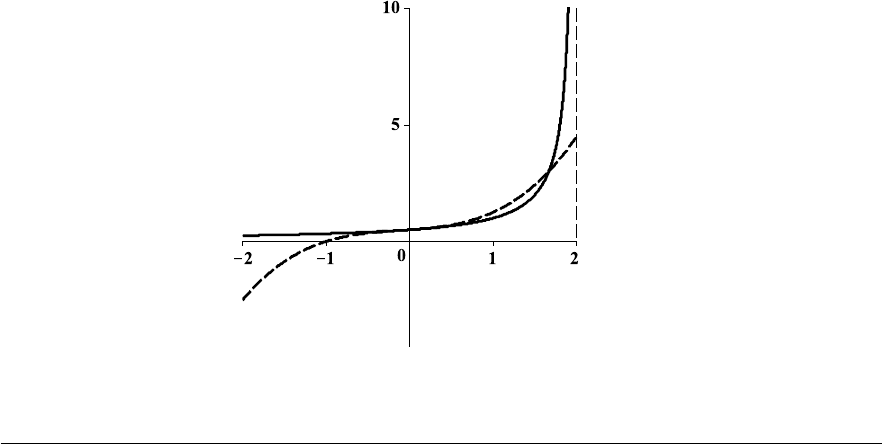
Chapter 8
FIGURES
Figure 8–A: The graphs of f(x) = 1/(2 − x) and its Taylor polynomial p
3
(x)
276

CHAPTER 9: Matrix Methods for Linear Systems
EXERCISES 9.1: Introduction
2.
"
x
y
#
0
=
"
0 1
−1 0
#"
x
y
#
4.
x
1
x
2
x
3
x
4
0
=
1 −1 1 −1
1 0 0 1
√
π 0 −1 0
0 0 0 0
x
1
x
2
x
3
x
4
6.
x
1
x
2
x
3
0
=
cos 2t 0 0
0 sin 2t 0
1 −1 0
x
1
x
2
x
3
8.
"
x
1
x
2
#
0
=
"
0 1
−2/(1 − t
2
) 2t/(1 − t
2
)
#"
x
1
x
2
#
10.
"
x
1
x
2
#
0
=
"
0 1
−1 + n
2
/t
2
−1/t
#"
x
1
x
2
#
12.
x
1
x
2
x
3
x
4
0
=
0 1 0 0
0 −3 −2 1
0 0 0 1
0 −1 −1 −3
x
1
x
2
x
3
x
4
EXERCISES 9.2: Review 1: Linear Algebraic Equations
2. x
1
= 0, x
2
=
1
3
, x
3
=
2
3
, x
4
= 0
4. x
1
=
1
3
, x
2
=
2
3
, x
3
= 0 , x
4
= 0
6. x
1
= −
s
4
, x
2
=
s
4
, x
3
= s (−∞ < s < ∞)
277

Chapter 9
8. x
1
= −s + t, x
2
= s, x
3
= t (−∞ < s, t < ∞)
10. x
1
=
−2 + i
5
, x
2
= 0, x
3
=
2 + 4i
5
12. (a) The equation produce the format
x
1
−
1
2
x
2
= 0,
0 = 1
(b) The equation produce the format
x
1
+
1
2
x
3
= 0,
x
2
+
11
3x
3
= 0,
0 = 1
14. For r = −1, the unique solution is x
1
= x
2
= x
3
= 0.
For r = 2, the solutions are x
1
= −
s
2
, x
2
=
s
4
, x
3
= s (−∞ < s < ∞).
EXERCISES 9.3: Review 2: Matrices and Vectors
2. (a) A + B =
"
3 −1 7
2 4 −1
#
(b) 7A − 4B =
"
10 4 27
14 −5 15
#
4. (a) AB =
2 5 −1
0 12 4
−1 8 4
(b) BA =
"
3 2
−1 15
#
6. (a) AB =
"
2 7
1 5
#
(b) (AB) C =
"
9 −1
6 1
#
(c) (A + B) C =
"
6 1
5 −5
#
278
Exercises 9.3
10.
9
31
−
1
31
−
5
31
4
31
12.
1 0 −1
1 −1 2
1 −1 1
14.
1
1
2
−
1
2
1
3
−
1
2
1
6
−
1
3
0
1
3
16. (c) x =
2
1
0
+ c
−1
−1
1
, with c arbitrary
18.
sin 2t
1
2
cos 2t
cos 2t −
1
2
sin 2t
20.
0 0
1
9
e
−3t
1 −t
1
3
t −
1
9
0 1 −
1
3
22. 0
24. 11
26. 54
28. 1, 6
279
Chapter 9
30. (b) 0
(c) x = c
1
1
−1
(d) c
1
= c
2
= c
3
= −1
32.
"
3e
−t
cos 3t − e
−t
sin 3t
−3e
−t
cos 3t + e
−t
sin 3t
#
34.
2 cos 2t −2 sin 2t −2e
−2t
−2 cos 2t −4 sin 2t −6e
−2t
6 cos 2t −2 sin 2t −2e
−2t
40. (a)
t −
1
2
e
−2t
3t −
1
2
e
−2t
+
"
c
11
c
12
c
21
c
22
#
(b)
"
−e
−1
+ 1 −e
−1
+ 1
e
−1
− 1 −3e
−1
+ 3
#
(c)
"
−e
−t
+ 3e
−3t
−3e
−t
− 9e
−3t
−3e
−t
+ 3e
−3t
−3e
−t
− 9e
−3t
#
42. In general, (AB)
T
= B
T
A
T
. Thus, (A
T
A)
T
= A
T
(A
T
)
T
= A
T
A, so A
T
A is symmetric.
Similarly, one shows that AA
T
is symmetric
EXERCISES 9.4: Linear Systems in Normal Form
2.
"
r
0
(t)
θ
0
(t)
#
=
"
2 0
1 −1
#"
r(t)
θ(t)
#
+
"
sin t
1
#
4.
dx
dt
dy
dt
dz
dt
=
1 1 1
2 −1 3
1 0 5
x
y
z
280
Exercises 9.4
6.
"
x
0
1
(t)
x
0
2
(t)
#
=
"
0 1
−1 0
#"
x
1
(t)
x
2
(t)
#
+
"
0
t
2
#
8.
x
0
1
(t)
x
0
2
(t)
x
0
3
(t)
=
0 1 0
0 0 1
−1 1 0
x
1
(t)
x
2
(t)
x
3
(t)
+
0
0
cos t
10. x
0
1
(t) = 2x
1
(t) + x
2
(t) + te
t
;
x
0
2
(t) = −x
1
(t) + 3x
2
(t) + e
t
12. x
0
1
(t) = x
2
(t) + t + 3;
x
0
2
(t) = x
3
(t) − t + 1;
x
0
3
(t) = −x
1
(t) + x
2
(t) + 2x
3
(t) + 2t
14. Linearly independent
16. Linearly dependent
18. Linearly independent
20. Yes.
"
3e
−t
e
4t
2e
−t
−e
4t
#
; c
1
"
3e
−t
2e
−t
#
+ c
2
"
e
4t
−e
4t
#
22. Linearly independent; fundamental matrix is
e
t
sin t −cos t
e
t
cos t sin t
e
t
−sin t cos t
The general solution is
c
1
e
t
e
t
e
t
+ c
2
sin t
cos t
−sin t
+ c
3
−cos t
sin t
cos t
24. c
1
e
3t
0
e
3t
+ c
2
−e
3t
e
3t
0
+ c
3
−e
−3t
−e
−3t
e
−3t
+
5t + 1
2t
4t + 2
281

Chapter 9
28. X
−1
(t) =
1
2
e
t
−
1
2
e
t
1
2
e
−5t
1
2
e
−5t
;
x(t) =
"
2e
−t
+ e
5t
−2e
−t
+ e
5t
#
32. Choosing x
0
= col(1, 0, 0, . . . , 0), then x
0
= col(0, 1, 0, . . . , 0), and so on, the correspond-
ing solutions x
1
, x
2
, . . . , x
n
will have a nonvanishing Wronskian at the initial point t
0
.
Hence, {x
1
, x
2
, . . . , x
n
} is a fundamental solution set
EXERCISES 9.5: Homogeneous Linear Systems with Constant Coefficients
2. Eigenvalues are r
1
= 3 and r
2
= 4 with associated eigenvectors
u
1
= s
"
1
1
#
and u
2
= s
"
3
2
#
4. Eigenvalues are r
1
= −4 and r
2
= 2 with associated eigenvectors
u
1
= s
"
1
−1
#
and u
2
= s
"
5
1
#
6. Eigenvalues are r
1
= r
2
= −1 and r
3
= 2 with associated eigenvectors
u
1
= s
−1
1
0
, u
2
= ν
−1
0
1
, and u
3
= s
1
1
1
8. Eigenvalues are r
1
= −1 and r
2
= −2 with associated eigenvectors
u
1
= s
1
2
4
and u
2
= s
1
1
1
10. Eigenvalues are r
1
= 1, r
2
= 1 + i, and r
3
= 1 − i with associated eigenvectors
u
1
= s
1
0
0
, u
2
= s
−1 − 2i
1
i
, and u
3
= s
−1 + 2i
1
−i
,
where s is any complex constant
282
Exercises 9.5
12. c
1
e
7t
"
1
2
#
+ c
2
e
−5t
"
1
−2
#
14. c
1
e
−t
−1
0
1
+ c
2
e
−2t
1
−1
3
+ c
3
e
3t
1
4
3
16. c
1
e
−10t
2
0
−1
+ c
2
e
5t
0
1
0
+ c
3
e
5t
1
0
2
18. (a) Eigenvalues are r
1
= −1 and r
2
= −3 with associated eigenvectors
u
1
= s
"
1
1
#
and u
2
= s
"
1
−1
#
(b)
(
x
1
= e
−t
x
2
= e
−t
(c)
(
x
1
= −e
−3t
x
2
= e
−3t
(d)
(
x
1
= e
−t
− e
−3t
x
2
= e
−t
+ e
−3t
See Figures 9–A, 9–B, and 9–C on page 290.
20.
"
e
t
4e
4t
−e
t
−e
4t
#
22.
e
2t
−e
2t
e
t
0 e
2t
e
t
e
2t
0 3e
t
24.
1 e
4t
0 0
4 0 0 0
0 0 3e
t
e
−t
0 0 e
t
e
−t
26. x(t) = c
1
e
−5t
+ 2c
2
e
t
;
y(t) = 2c
1
e
−5t
+ c
2
e
t
28.
−0.2931e
0.4679t
0.4491e
3.8794t
−0.6527e
1.6527t
−0.5509e
0.4679t
−0.1560e
3.8794t
e
1.6527t
e
0.4679t
e
3.8794t
−0.7733e
1.6527t
283
Chapter 9
30.
e
0.6180t
−0.6180e
−1.6180t
0 0
−0.6180e
0.6180t
e
−1.6180t
0 0
0 0 e
0.5858t
0.2929e
3.4142t
0 0 0.5858e
0.5858t
e
3.4142t
32.
"
2e
3t
− 12e
4t
2e
3t
− 8e
4t
#
34.
e
2t
− 2e
−t
e
2t
+ 3e
−t
e
2t
− e
−t
36. c
1
e
2t
"
1
1
#
+ c
2
(
te
2t
"
1
1
#
+ e
2t
"
4/3
1
#)
38. c
1
e
t
1
1
0
+ c
2
te
t
1
1
0
+ e
t
0
0
1
+ c
3
t
2
e
t
2
1
1
0
+ te
t
0
0
1
+ e
t
−1/4
0
1/2
40. c
1
e
t
1
0
0
+ c
2
e
t
0
2
3
+ c
3
te
t
1
2
3
+ e
t
0
1
1
44. c
1
"
1
2
#
+ c
2
t
−5
"
−2
1
#
46. x
1
(t) =
e
−3t
10
kg, x
2
(t) =
3 − α
10α
(e
αt
− 1)e
−3t
kg
The mass of salt in tank A is independent of α. The maximum mass of salt in tank B
is 0.1
3 − α
3
3/α
kg
50. (b) x(t) = 1 +
3
2
e
−t
+
1
2
e
−3t
;
y(t) = 1 − e
−3t
;
z(t) = 1 −
3
2
e
−t
+
1
2
e
−3t
284
Exercises 9.6
EXERCISES 9.6: Complex Eigenvalues
2. c
1
"
−5 cos t
2 cos t − sin t
#
+ c
2
"
−5 sin t
2 sin t + cos t
#
4. c
1
5e
2t
cos t
−2e
2t
cos t + e
2t
sin t
5e
2t
cos t
+ c
2
5e
2t
sin t
−2e
2t
sin t − e
2t
cos t
5e
2t
sin t
+ c
3
0
e
2t
−e
2t
6.
"
cos 2t sin 2t
sin 2t − cos 2t −sin 2t − cos 2t
#
8.
e
t
e
−t
0 0
e
t
e
−t
0 0
0 0 e
2t
cos 3t e
2t
sin 3t
0 0 e
2t
(2 cos 3t − 3 sin 3t) e
2t
(2 sin 3t + 3 cos 3t)
10.
−0.0209e
2t
cos 3t + 0.0041e
2t
sin 3t −0.0209e
2t
sin 3t − 0.0041e
2t
cos 3t −e
−t
e
t
−0.0296e
2t
cos 3t + 0.0710e
2t
sin 3t −0.0296e
2t
sin 3t − 0.0710e
2t
cos 3t e
−t
e
t
0.1538e
2t
cos 3t + 0.2308e
2t
sin 3t 0.1538e
2t
sin 3t − 0.2308e
2t
cos 3t −e
−t
e
t
e
2t
cos 3t e
2t
sin 3t −e
−t
e
t
12.
0 0 0 0 e
t
0 0 e
−t
e
t
0
0 0 −e
−t
e
t
0
−0.07e
−2t
cos 5t + 0.17e
−2t
sin 5t −0.067e
−2t
sin 5t − 0.17e
−2t
cos 5t 0 0 0
e
−2t
cos 5t e
−2t
sin 5t 0 0 0
14. (a)
e
t
sin t − 2e
t
cos t
2e
2t
−e
t
cos t − 2e
t
sin t
(b)
e
t+π
sin t
e
2(t+π)
−e
t+π
cos t
18. c
1
t
−1
"
cos(3 ln t)
3 sin(3 ln t)
#
+ c
2
t
−1
"
sin(3 ln t)
−3 cos(3 ln t)
#
285
Chapter 9
20. x
1
(t) = cos t −cos
√
3 t;
x
2
(t) = cos t + cos
√
3 t
22. I
1
(t) =
16
5
e
−2t
−
1
5
e
−8t
+ 2;
I
2
(t) = 4e
−2t
− e
−8t
+ 2;
I
3
(t) = −
4
5
e
−2t
+
4
5
e
−8t
EXERCISES 9.7: Nonhomogeneous Linear Systems
2. c
1
"
e
3t
2e
3t
#
+ c
2
"
e
−t
−2e
−t
#
+
"
t
2
#
4. c
1
"
1
−1
#
+ c
2
"
e
4t
e
4t
#
+
"
−2 sin t
2 sin t + cos t
#
6. x
p
= ta + b + e
3t
c
8. x
p
= t
2
a + tb + c
10. x
p
= e
−t
a + te
−t
b
12. c
1
e
4t
"
2
3
#
+ c
2
e
−t
"
1
−1
#
+
"
1
−1
#
14. c
1
"
cos t
sin t
#
+ c
2
"
−sin t
cos t
#
+
"
2t − 1
t
2
− 2
#
16. c
1
"
cos t
−sin t
#
+ c
2
"
sin t
cos t
#
+
"
4t sin t
4t cos t − 4 s in t
#
18. c
1
e
t
1
0
0
+ c
2
e
t
0
1
1
+ c
3
e
t
t
t
t + 1
+
−te
t
− e
t
0
−e
t
20.
−c
1
sin 2t + c
2
cos 2t − c
3
e
−2t
+ 8c
4
e
t
+ (8/15) te
t
+ (17/225) e
t
− (1/8)
−2c
1
cos 2t − 2c
2
sin 2t + 2c
3
e
−2t
+ 8c
4
e
t
+ (8/15) te
t
− (88/225) e
t
4c
1
sin 2t − 4c
2
cos 2t − 4c
3
e
−2t
+ 8c
4
e
t
+ (8/15) te
t
+ (32/225) e
t
8c
1
cos 2t + 8c
2
sin 2t + 8c
3
e
−2t
+ 8c
4
e
t
+ (8/15) te
t
+ (152/225) e
t
− 1
286
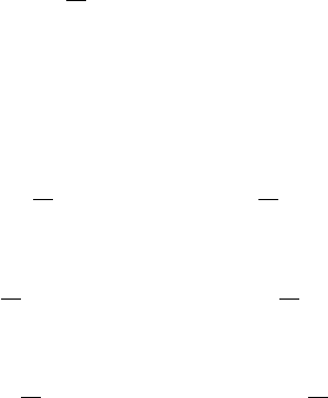
Exercises 9.8
22. (a)
"
3e
−4t
+ e
2t
−6e
−4t
+ e
2t
− 2t
#
(b)
"
−(4/3) e
−4(t−2)
+ (7/3) e
2(t−2)
(8/3) e
−4(t−2)
+ (7/3) e
2(t−2)
− 2t
#
24. x(t) = 3e
−4t
+ e
2t
;
y(t) = −6e
−4t
+ e
2t
− 2t;
26. (a)
"
e
t
−2e
t
#
(b)
"
te
t
te
t
#
28.
"
−t + 1
−t − 1
#
30. c
1
t
−2
"
1
2
#
+ c
2
"
3
4
#
+ t
"
1/3
2/3
#
34. (a) Neither wins.
(b) The x
1
force wins.
(c) The x
2
force wins.
EXERCISES 9.8: The Matrix Exponential Function
2. (a) r = 2; k = 2 (b) e
2t
"
1 − t −t
t 1 + t
#
4. (a) r = 2; k = 3
(b) e
2t
1 t 3t −
t
2
2
0 1 −t
0 0 1
6. (a) r = −1; k = 3
(b) e
−t
1 + t +
t
2
2
t + t
2
t
2
2
−
t
2
2
1 + t − t
2
t −
t
2
2
−t +
t
2
2
−3t + t
2
1 − 2t +
t
2
2
287

Chapter 9
8.
"
(1/2) e
3t
+ (1/2) e
−t
(1/4) e
3t
− (1/4) e
−t
e
3t
− e
−t
(1/2) e
3t
+ (1/2) e
−t
#
10.
1
3
e
4t
+ 2e
−2t
e
4t
− e
−2t
e
4t
− e
−2t
e
4t
− e
−2t
e
4t
+ 2e
−2t
e
4t
− e
−2t
e
4t
− e
−2t
e
4t
− e
−2t
e
4t
+ 2e
−2t
12.
1
9
3e
−t
+ 6e
2t
−3e
−t
+ 3e
2t
−3e
−t
+ 3e
2t
−4e
−t
+ 4e
2t
+ 6te
2t
4e
−t
+ 5e
2t
+ 3te
2t
4e
−t
− 4e
2t
+ 3te
2t
−2e
−t
+ 2e
2t
− 6te
2t
2e
−t
− 2e
2t
− 3te
2t
2e
−t
+ 7e
2t
− 3te
2t
14.
e
t
0 0 0 0
0 e
t
+ te
−t
te
−t
0 0
0 −te
−t
e
−t
− te
−t
0 0
0 0 0 cos t sin t
0 0 0 −sin t cos t
16.
e
−t
0 0 0 0
0 e
−t
+ te
−t
te
−t
0 0
0 −te
−t
e
−t
− te
−t
0 0
0 0 0 e
−2t
+ 2te
−2t
te
−t
0 0 0 −4te
−2t
e
−2t
− 2te
−2t
18. c
1
1
0
0
+ c
2
e
t
0
1
0
+ c
3
e
t
1
2t
1
20. c
1
e
t
−4
1
0
+ c
2
e
t
3 − 4t
t
2
+ c
3
e
t
1 − 2t + 4t
2
−t − t
2
−4t
22.
−(4/3) e
−t
+ (1/3) e
2t
(16/9) e
−t
− (16/9) e
2t
+ (1/3) te
2t
(8/9) e
−t
+ (19/9) e
2t
− (1/3) te
2t
24.
e
t
+ cos t − sin t − 1 − t
e
t
− sin t − cos t − 1
e
t
− cos t + sin t
288

Review problems
REVIEW PROBLEMS
2. c
1
e
2t
"
−2 cos 3t
cos 3t + 3 sin 3t
#
+ c
2
e
2t
"
−2 sin 3t
sin 3t − 3 cos 3t
#
4. c
1
e
2t
0
0
1
+ c
2
e
t
1
0
0
+ c
3
t
1
0
6.
0 e
5t
0
3e
−5t
0 e
5t
−e
−5t
0 3e
5t
8. c
1
"
1
2
#
+ c
2
"
2e
−5t
−e
−5t
#
+ e
4t
"
11/36
13/18
#
10. c
1
e
2t
1
0
0
+ c
2
e
5t/2
cos
√
7 t
2
!
11
−2
4
− e
5t/2
sin
√
7 t
2
!
−3
√
7
−2
√
7
0
+c
3
e
5t/2
sin
√
7 t
2
!
11
−2
4
+ e
5t/2
cos
√
7 t
2
!
−3
√
7
−2
√
7
0
+
−(1/3) e
−t
+ 11/16
−1/4
−5/8
12.
"
e
2t
sin 2t + (3/2) e
2t
cos 2t + (1/2) e
2t
2e
2t
cos 2t − 3e
2t
sin 2t − te
2t
#
14. c
1
t
−1
1
2
+ c
2
t
3
1
1
0
+ c
3
t
−2
1
−1
1
16.
1 t 4t + t
2
0 1 2t
0 0 1
289
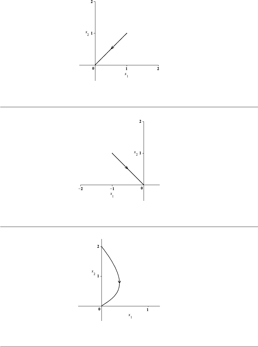
Chapter 9
FIGURES
Figure 9–A: Problem 18(b), Section 9.5
Figure 9–B: Problem 18(c), Section 9.5
Figure 9–C: Problem 18(d), Section 9.5
290

CHAPTER 10: Partial Differential Equations
EXERCISES 10.2: Method of Separation of Variables
2. y =
(e
10
− 1) e
x
+ (1 − e
2
) e
5x
e
10
− e
2
4. y = 2 sin 3x
6. No solution
8. y = e
x−1
+ xe
x−1
10. λ
n
=
(2n − 1)
2
4
and y
n
= c
n
cos
2n − 1
2
x
, where n = 1, 2, 3, . . . and c
n
’s are arbitrary
12. λ
n
= 4n
2
and y
n
= c
n
cos(2nx), where n = 0, 1, 2, . . . and c
n
’s are arbitrary
14. λ
n
= n
2
+ 1 and y
n
= c
n
e
x
sin(nx), where n = 1, 2, 3, . . . and c
n
’s are arbitrary
16. u(x, t) = e
−27t
sin 3x + 5e
−147t
sin 7x − 2e
−507t
sin 13x
18. u(x, t) = e
−48t
sin 4x + 3e
−108t
sin 6x − e
−300t
sin 10x
20. u(x, t) = −
2
9
sin 9t sin 3x +
3
7
sin 21t sin 7x −
1
30
sin 30t sin 10x
22. u(x, t) = cos 3t sin x−cos 6t sin 2x+cos 9t sin 3x+
2
3
sin 9t sin 3x−
7
15
sin 15t sin 5x
24. u(x, t) =
∞
X
n=1
1
n
2
cos 4nt +
(−1)
n+1
4n
2
sin 4nt
sin nx
EXERCISES 10.3: Fourier Series
2. Even
4. Neither
6. Odd
291

Chapter 10
10. f (x) ∼
π
2
−
4
π
∞
X
k=0
1
(2k + 1)
2
cos(2k + 1)x
12. f (x) ∼
π
2
6
+
∞
X
n=1
2(−1)
n
n
2
cos nx +
(−1)
n
(2 − n
2
π
2
) − 2
πn
3
sin nx
14. f (x) ∼
π
2
+
∞
X
n=1
1
n
sin 2nx
16. f (x) ∼
∞
X
n=1
2 [1 − cos (πn/2)]
πn
sin nx
18. The 2π-periodic function g(x), where g(x) = |x| on −π ≤ x ≤ π
20. The 2π-periodic function g(x), where g(x) =
0, −π < x ≤ 0
x
2
, 0 < x < π
π
2
/2, x = ±π
22. The 2π-periodic function g(x), where g(x) =
x + π, −π < x < 0
x, 0 < x < π
π/2, x = 0, ±π
24. The 2π-periodic function g(x), where g(x) =
0, −π ≤ x < −π/2
−1/2, x = −π/2
−1, −π/2 < x < 0
0, x = 0
1, 0 < x < π/2
1/2, x = π/2
0, π/2 < x ≤ π
30. a
0
=
1
2
, a
1
= 0, a
2
=
5
8
EXERCISES 10.4: Fourier Cosine and Sine Series
2. (a) The π-periodic function
e
f(x) = sin 2x for x 6= kπ, where k is an integer
(b) The 2π-periodic function f
o
(x) = sin 2x for x 6= kπ, where k is an integer
(c) The 2π-periodic function f
e
(x), where f
e
(x) =
(
−sin 2x, −π < x < 0
sin 2x, 0 < x < π
292
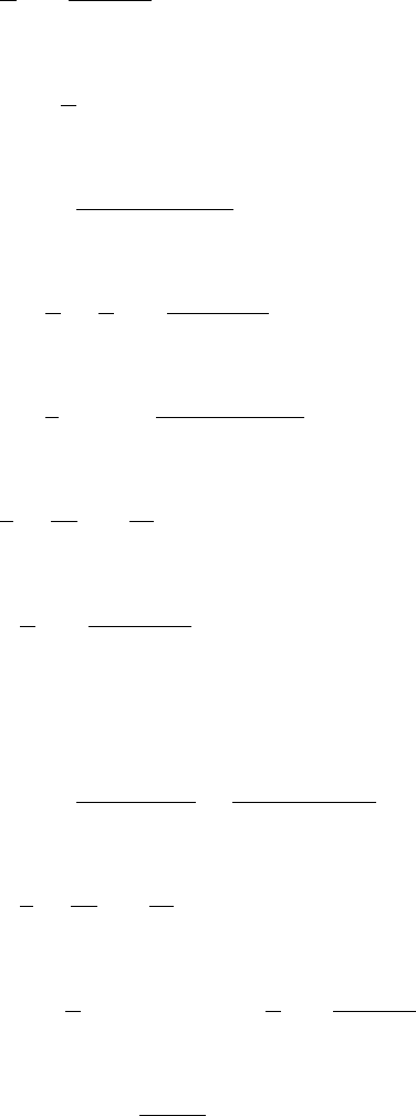
Exercises 10.5
4. (a) The π-periodic function
e
f(x), where
e
f(x) = π − x, 0 < x < π
(b) The 2π-periodic function f
o
(x), where f
o
(x) =
(
−π − x, −π < x < 0
π − x, 0 < x < π
(c) The 2π-periodic function f
e
(x), where f
e
(x) =
(
π + x, −π < x < 0
π − x, 0 < x < π
6. f (x) ∼
8
π
∞
X
k=1
k
4k
2
− 1
sin(2kx)
8. f (x) ∼ 2
∞
X
n=1
1
n
sin(nx)
10. f (x) ∼ 2π
∞
X
n=1
n [1 − e(−1)
n
]
1 + π
2
n
2
sin(πnx)
12. f (x) ∼ 1 +
π
2
−
4
π
∞
X
k=0
1
(2k + 1)
2
cos [(2k + 1)x]
14. f (x) ∼ 1 −
1
e
+ 2
∞
X
n=1
1 − (−1)
n
e
−1
1 + π
2
n
2
cos (πnx)
16. f (x) ∼
1
6
−
1
π
2
∞
X
k=1
1
k
2
cos (2πkx)
18. u(x, t) =
8
π
∞
X
k=0
1
(2k + 1)
3
e
−5(2k+1)
2
t
sin [(2k + 1)x]
EXERCISES 10.5: The Heat Equation
2. u(x, t) =
∞
X
n=1
2π(−1)
n+1
n
+
4 [(−1)
n
− 1]
πn
3
e
−n
2
t
sin (nx)
4. u(x, t) =
1
6
−
1
π
2
∞
X
k=1
1
k
2
e
−8π
2
k
2
t
cos (2πkx)
6. u(x, t) = 1 −
2
π
+ 2e
−7t
cos x +
4
π
∞
X
k=1
1
4k
2
− 1
e
−28k
2
t
cos (2kx)
8. u(x, t) = 3x + 6
∞
X
n=1
(−1)
n
n
e
−n
2
t
sin (nx)
293
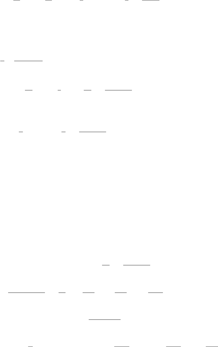
Chapter 10
10. u(x, t) =
π
2
18
x −
1
18
x
3
+
1
3
e
−3t
sin x +
2
3
∞
X
n=2
(−1)
n
n
3
e
−3n
2
t
sin (nx)
12. u(x, t) =
∞
X
n=1
a
n
e
−µ
2
n
t
sin (µ
n
x), where {µ
n
}
∞
n=1
is the increasing sequence of p ositive real
numbers that are solutions to tan (µ
n
π) = −µ
n
, and
a
n
=
π
2
−
sin(2πµ
n
)
4
−1
π
Z
0
f(x) sin (µ
n
x) dx
14. u(x, t) = 1 +
5π
6
x −
5
6
x
2
−
20
3π
∞
X
k=0
1
(2k + 1)
3
e
−3(2k+1)
2
t
sin [(2k + 1)x]
16. u(x, y, t) = e
−2t
cos x sin y + 4e
−5t
cos 2x sin y − 3e
−25t
cos 3x sin 4y
18. u(x, y, t) =
π
2
e
−t
sin y −
4
π
∞
X
k=0
1
(2k + 1)
2
e
−
[
(2k+1)
2
+1
]
t
cos [(2k + 1)x] sin y
EXERCISES 10.6: The Wave Equation
2. u(x, t) =
∞
X
n=1
(a
n
cos 4nt + b
n
sin 4nt) sin nx, where
a
n
=
(
0, n even
(2/π) [n/ (n
2
− 4) − 1/n] , n odd
and
b
n
=
(
−1/ [4π (n
2
− 1)] , n even
1/(πn
2
), n odd
4. u(x, t) = sin 4x cos 12t + 7 sin 5x cos 15t +
4
3π
∞
X
k=0
(−1)
k
(2k + 1)
3
sin [(2k + 1)x] sin [3(2k + 1)t]
6. u(x, t) =
2ν
0
L
3
π
3
αa(L −a)
∞
X
n=1
1
n
3
sin
nπa
L
sin
nπx
L
sin
nπαt
L
8. u(x, t) = sin x (sin t −t cos t) + 2
∞
X
n=2
(−1)
n
n
2
(n
2
− 1)
(sin nt − n sin t) sin nx
10. u(x, t) = U
1
+
x
L
(U
2
− U
1
) +
∞
X
n=1
a
n
cos
παnt
L
+ b
n
sin
παnt
L
sin
πnx
L
,
where a
n
’s and b
n
’s are chosen that
294

Exercises 10.7
f(x) =
∞
X
n=1
a
n
sin
πnx
L
+ U
1
+
x
L
(U
2
− U
1
)
g(x) =
∞
X
n=1
b
n
παn
L
sin
πnx
L
14. u(x, t) = x
2
+ α
2
t
2
16. u(x, t) = sin 3x cos 3αt + t
18. u(x, t) = cos 2x cos 2αt + t −xt
EXERCISES 10.7: Laplace’s Equation
2. u(x, y) =
cos x sinh(y − π)
sinh(−π)
−
2 cos 4x sinh(4y − 4π)
sinh(−4π)
4. u(x, y) =
sin x sinh(y − π)
sinh(−π)
+
sin 4x sinh(4y − 4π)
sinh(−4π)
8. u(r, θ) =
1
2
+
r
2
8
cos 2θ
12. u(r, θ) =
3
3
3
6
− 1
r
3
− r
−3
cos 3θ +
3
5
3
10
− 1
r
5
− r
−5
cos 5θ
14. u(r, θ) = C +
∞
X
n=1
r
−n
(a
n
cos nθ + b
n
sin nθ),
where C is arbitrary and, for n = 1, 2, . . . ,
a
n
= −
1
πn
π
Z
−π
f(θ) cos nθ dθ ,
b
n
= −
1
πn
π
Z
−π
f(θ) sin nθ dθ
16. u(r, θ) =
∞
X
n=1
a
n
sinh
π(θ − π)n
ln 2
sin
π(ln r − ln π)n
ln 2
, where
a
n
= −
2
(ln 2) sinh (nπ
2
/ ln 2)
2π
Z
π
(sin r) sin
π(ln r − ln π)n
ln 2
dr
r
295

Chapter 10
24. u(x, y) =
∞
X
n=1
A
n
e
−ny
sin nx,
where A
n
=
2
π
π
Z
0
f(x) sin nx dx
296

CHAPTER 11: Eigenvalue Problems and
Sturm-Liouville Equations
EXERCISES 11.2: Eigenvalues and Eigenfunctions
2. sin x − cos x + x + 1
4. ce
−2x
(sin 2x + cos 2x)
6. 2e
x
+ e
−x
− x
8. c
1
sin 2x + c
2
cos 2x + 1
10. No solution
12. No solution
14. λ
n
=
π
2
n
2
9
; y
n
(x) = b
n
sin
πnx
3
+ c
n
cos
πnx
3
, n = 0, 1, 2, . . .
16. λ
n
= 2 +
(2n + 1)
2
4
; y
n
(x) = c
n
sin
(2n + 1) x
2
, n = 0, 1, 2, . . .
18. λ
0
= −µ
2
0
, where tanh (µ
0
π) = 2µ
0
; y
0
(x) = c
0
sinh (µ
0
x);
λ
n
= µ
2
n
, where tan (µ
n
π) = 2µ
n
; y
n
(x) = c
n
sin (µ
n
x), n = 1, 2, 3, . . .
20. λ
n
= π
2
n
2
, y
n
(x) = c
n
cos (πn ln x), n = 0, 1, 2, . . .
22. λ
1
= 4.116, λ
2
= 24.139, λ
3
= 63.659
24. No nontrivial solutions
26. λ
n
= µ
2
n
, where cot (µ
n
π) = µ
n
for µ
n
> 0; y
n
(x) = c
n
sin (µ
n
x), n = 1, 2, 3, . . .
28. λ
n
= −µ
4
n
, µ
n
> 0 and cos (µ
n
L) cosh (µ
n
L) = −1;
y
n
= c
n
sin (µ
n
x) − sinh (µ
n
x) −
sin (µ
n
L) + sinh (µ
n
L)
cos (µ
n
L) + cosh (µ
n
L)
(cos (µ
n
x) − cosh (µ
n
x))
,
n = 1, 2, 3, . . .
297

Chapter 11
34. (b) λ
0
= −1, X
0
(x) = c and λ
n
= −1 + n
2
π
2
, X
n
(x) = c cos (πnx)
EXERCISES 11.3: Regular Sturm-Liouville Boundary Value Problems
2. y
00
+ λx
−1
y = 0
4. (xy
0
)
0
+ xy − λx
−1
y = 0
6. [(1 − x
2
) y
0
]
0
+ λy = 0
8. Ye s
10. No
18. (a)
1
√
6
,
1
√
3
sin
nπx
3
,
1
√
3
cos
nπx
3
, n = 1, 2, 3, . . .
(b)
∞
X
n=1
(−1)
n+1
6
πn
sin
nπx
3
20. (a)
r
2
π
sin
n +
1
2
x
, n = 0, 1, 2, . . .
(b)
∞
X
n=0
(−1)
n
8
π (2n + 1)
2
sin
n +
1
2
x
22. (a) 2
r
µ
0
sinh (2µ
0
π) − 2µ
0
π
sinh (µ
0
x), where tanh (µ
0
π) = 2µ
0
;
2
r
µ
n
2µ
n
π − sin (2µ
n
π)
sin (µ
n
x), where tan (µ
n
π) = 2µ
n
, n = 1, 2, 3, . . .
(b)
4 (π − 2) cosh (µ
0
π)
sinh (2µ
0
π) − 2µ
0
π
sinh (µ
0
π) +
∞
X
n=1
4(2 − π) cos (µ
n
π)
2µ
n
π − sin (2µ
n
π)
sin (µ
n
x)
24. (a) y
0
(x) =
1
√
e − 1
; y
n
(x) =
√
2 cos (πn ln x), n = 1, 2, 3, . . .
(b) 1 +
∞
X
n=1
2 [(−1)
n
e − 1]
1 + π
2
n
2
cos (πn ln x)
EXERCISES 11.4: Nonhomogeneous Boundary Value Problems and the
Fredholm Alternative
2. L
+
[y] = x
2
y
00
+ (4x − sin x) y
0
+ (2x + 2 − cos x) y
298
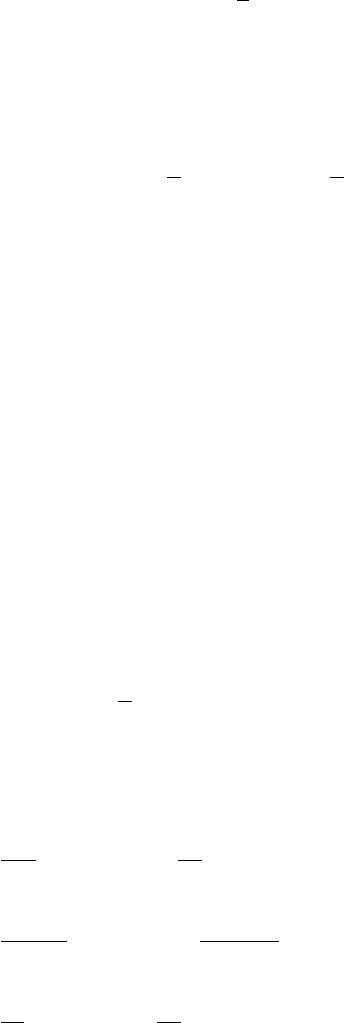
Exercises 11.5
4. L
+
[y] = x
2
y
00
+ 6xy
0
+ 7y
6. L
+
[y] = (sin x) y
00
+ (2 cos x + e
x
) y
0
+ (−sin x + e
x
+ 1)y
8. L
+
[y] = y
00
+ 4y
0
+ 5y;
D (L
+
) = {y ∈ C
2
[0, 2π] : y(0) = y(2π) = 0}
10. L
+
[y] = x
2
y
00
+ 2xy
0
+
5
4
y;
D (L
+
) = {y ∈ C
2
[1, e
π
] : y(1) = y(e
π
) = 0}
12. y
00
− y
0
+ y = 0; y(0) = y(π), y
0
(0) = y
0
(π)
14. y
00
= 0; y(0) = y
π
2
, y
0
(0) = y
0
π
2
16. x
2
y
00
+ 2xy
0
= 0; y(1) = 4y(2), y
0
(1) = 4y
0
(2)
18.
2π
Z
0
h(x)e
−2x
sin x dx = 0
20.
e
π
Z
1
h(x)x
−1/2
sin(ln x) dx = 0
22. Unique solution for each h
24.
π/2
Z
0
h(x) dx = 0
26.
2
Z
1
h(x)
1 −
3
x
dx = 0
EXERCISES 11.5: Solution by Eigenfunction Expansion
2.
1
122
sin 11x −
1
17
sin 4x
4.
1
π − 49
cos 7x +
5
π − 100
cos 10x
6.
1
19
cos 5x −
1
10
cos 4x
299

Chapter 11
8.
∞
X
n=0
−8
π(2n + 1)
3
(4n
2
+ 4n − 1)
sin[(2n + 1)x]
10.
∞
X
n=0
γ
n
7 −
n +
1
2
2
sin
n +
1
2
x
, where γ
n
=
2
π
π
Z
0
f(x) sin
n +
1
2
x
dx
12. Let γ
n
=
2
π
e
π
Z
1
f(x) sin(n ln x) dx.
If γ
1
6= 0, there is no solution.
If γ
1
= 0, then
c sin(ln x) +
∞
X
n=2
γ
n
1 − n
2
sin(n ln x) is a solution
14.
∞
X
n=0
γ
n
−1 − π
2
n
2
cos(πn ln x), where γ
n
=
e
R
1
f(x) cos(πn ln x) dx
e
R
1
x
−1
cos
2
(πn ln x) dx
EXERCISES 11.6: Green’s Functions
2. G(x, s) =
−
sinh s sinh(x − 1)
sinh 1
, 0 ≤ s ≤ x
−
sinh x sinh(s − 1)
sinh 1
, x ≤ s ≤ 1
4. G(x, s) =
(
−cos s sin x , 0 ≤ s ≤ x
−cos x sin s , x ≤ s ≤ π
6. G(x, s) =
(
(sin s − cos s) sin x , 0 ≤ s ≤ x
(sin x − cos x) sin s , x ≤ s ≤ π
8. G(x, s) =
−
(s
2
+ s
−2
) (x
2
− 16x
−2
)
68
, 0 ≤ s ≤ x
−
(x
2
+ x
−2
) (s
2
− 16s
−2
)
68
, x ≤ s ≤ 2
300

Exercises 11.6
10. G(x, s) =
(e
5s
− e
−s
) (5e
6−x
+ e
5x
)
30e
6
+ 6
, 0 ≤ s ≤ x
(e
5x
− e
−x
) (5e
6−s
+ e
5s
)
30e
6
+ 6
, x ≤ s ≤ 1
12. G(x, s) =
−
s(x − π)
π
, 0 ≤ s ≤ x
−
x(s − π)
π
, x ≤ s ≤ π
y =
x
4
− π
3
x
12
14. G(x, s) =
(
s , 0 ≤ s ≤ x
x , x ≤ s ≤ π
y =
4π
3
x − x
4
12
16. G(x, s) =
−
sin s sin(x − 2)
sin 2
, 0 ≤ s ≤ x
−
sin x sin(s − 2)
sin 2
, x ≤ s ≤ 2
y =
12
sin 2
[sin x − sin(x − 2) − sin 2]
18. G(x, s) =
cosh s cosh(x − 1)
sinh 1
, 0 ≤ s ≤ x
cosh x cosh(s − 1)
sinh 1
, x ≤ s ≤ 1
y = −24
20. G(x, s) =
−
1 −
1
s
1 −
2
x
, 1 ≤ s ≤ x
−
1 −
1
x
1 −
2
s
, x ≤ s ≤ 2
y =
2 ln 2
x
+ ln
x
4
24. (a) K(x, s) =
(
e
x−s
s(1 − x) , 0 ≤ s ≤ x
e
x−s
x(1 − s) , x ≤ s ≤ 1
(b) y = (x −1)e
x
− xe
x−1
+ 1
301

Chapter 11
26. (a) K(x, s) =
(s
2
− s
−2
) (3x + 16x
−3
)
76
, 1 ≤ s ≤ x
(x − x
−3
) (3s
2
+ 16s
−2
)
76
, x ≤ s ≤ 2
(b) y =
1
4
x ln x +
4(1 + ln 2)
19
(x
−3
− x)
28. H(x, s) =
x(π − s)(s
2
− 2πs + x
2
6π
, 0 ≤ s ≤ x
s(π − x)(x
2
− 2πx + s
2
)
6π
, x ≤ s ≤ π
30. H(x, s) =
x
2
[(x − 3π)(s
3
− 3πs
2
) + 2π
3
(x − 3s)]
12π
3
, 0 ≤ s ≤ x
s
2
[(s − 3π)(x
3
− 3πx
2
) + 2π
3
(s − 3x)]
12π
3
, x ≤ s ≤ π
EXERCISES 11.7: Singular Sturm-Liouville Boundary Value Problems
2.
∞
X
n=1
b
n
J
3
(α
3n
x), where {α
3n
} is the increasing sequence of real zeros of J
3
and
b
n
=
1
R
0
f(x)J
3
(α
3n
x) dx
(µ − α
2
3n
)
1
R
0
J
2
3
(α
3n
x)x dx
4.
∞
X
n=0
b
n
P
n
(x), where
b
n
=
1
R
−1
f(x)P
n
(x) dx
[µ − n(n + 1)]
1
R
−1
P
2
n
(x) dx
6.
∞
X
n=0
b
n
P
2n
(x), where
b
n
=
1
R
0
f(x)P
2n
(x) dx
[µ − 2n(2n + 1)]
1
R
0
P
2
2n
(x) dx
302

Review Problems
16. (c)
∞
X
n=0
b
n
L
n
(x), where
b
n
=
∞
R
0
f(x)L
n
(x) dx
(µ − n)
∞
R
0
L
2
n
(x)e
−x
dx
EXERCISES 11.8: Oscillation and Comparison Theory
2. No; sin x has a finite number of zeros on any closed bounded interval.
4. No; it has an infinite number of zeros on the interval
−
1
2
,
1
2
8.
π
3
10. Between π
r
e
−25
λ + 1
and π
r
26
λ + 26 sin 5
REVIEW PROBLEMS
2. (a) (e
7x
y
0
)
0
+ λe
7x
y = 0
(b)
e
−3x
2
/2
y
0
0
+ λe
−3x
2
/2
y = 0
(c) (xe
−x
y
0
)
0
+ λe
−x
y = 0
4. (a) y
00
− xy
0
= 0; y
0
(0) = 0, y
0
(1) = 0
(b) x
2
y
00
+ 2xy
0
− 3y = 0; y(1) = 0, y
0
(e) = 0
6.
π
6
+ 4 cos 2x +
2
π
∞
X
k=0
1
(2k
2
+ 2k − 1) (2k + 1)
2
cos[(2k + 1)x]
8. (a)
∞
X
n=1
b
n
J
7
(α
7n
x), where {α
7n
} is the increasing sequence of real zeros of J
7
and
b
n
=
1
R
0
f(x)J
7
(α
7n
x) dx
(µ − α
2
7n
)
1
R
0
J
2
7
(α
7n
x)x dx
(b)
∞
X
n=0
b
n
P
n
(x), where
303
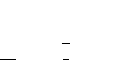
Chapter 11
b
n
=
1
R
−1
f(x)P
n
(x) dx
[µ − n(n + 1)]
1
R
−1
P
2
n
(x) dx
10. Between
π
√
6
and π
r
3
5
304
CHAPTER 12: Stability of Autonomous Systems
EXERCISES 12.2: Linear Systems in the Plane
2. Unstable proper node
4. Unstable improper node
6. Stable center
8. (−1, −1) is an asymptotically stable spiral point
10. (2, −2) is an unstable spiral point
12. (5, 1) is an asymptotically stable improper node
14. Unstable proper node. See Fig. 12–A on page 309.
16. Asymptotically stable spiral point. See Fig. 12–B on page 309.
18. Unstable improper node. See Fig. 12–C on page 309.
20. Stable center. See Fig. 12–D on page 310.
EXERCISES 12.3: Almost Linear Systems
2. Asymptotically stable improper node
4. Asymptotically stable spiral point
6. Unstable saddle point
8. Asymptotically stable improper node
10. (0, 0) is indeterminant; (−1, 1) is an unstable saddle point
12. (2, 2) is an asymptotically stable spiral point; (−2, −2) is an unstable saddle point
305
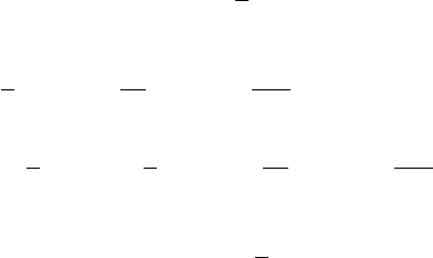
Chapter 12
14. (3, 3) is an unstable saddle point; (−2, −2) is an asymptotically stable spiral point. See
Fig. 12–E on page 310.
16. (0, 0) is an unstable saddle point; (−4, −2) is an asymptotically stable spiral point. See
Fig. 12–F on page 310.
EXERCISES 12.4: Energy Methods
2. G(x) = sin x + C; E(x, v) =
1
2
v
2
+ sin x
4. G(x) =
1
2
x
2
−
1
24
x
4
+
1
720
x
6
+ C;
E(x, v) =
1
2
v
2
+
1
2
x
2
−
1
24
x
4
+
1
720
x
6
6. G(x) = e
x
− x + C; E(x, v) =
1
2
v
2
+ e
x
− x − 1
8. See Fig. 12–G on page 311.
10. See Fig. 12–H on page 311.
12. See Fig. 12–I on page 312.
14. vh(x, v) = v
2
, so energy decreasing along a trajectory. See Fig. 12–A on page 312.
16. vh(x, v) = v
2
, so energy decreasing along a trajectory. See Fig. 12–B on page 313.
18. See Fig. 12–C on page 313.
EXERCISES 12.5: Lyapunov’s Direct Method
2. Asymptotically stable
4. Stable
6. Unstable
8. Asymptotically stable
10. Stable
306
Exercises 12.7
12. Stable
14. Stable
EXERCISES 12.6: Limit Cycles and Periodic Solutions
4. (b) Clockwise
6. r = 0 is an uns table spiral point; r = 2 is a stable limit cycle; r = 5 is an unstable limit
cycle. See Fig. 12–M on page 314.
8. r = 0 is an unstable spiral point. See Fig. 12–N on page 314.
10. r = 0 is an unstable spiral point; r = 2 is a stable limit cycle; r = 3 is a unstable limit
cycle. See Fig. 12–O on page 314.
12. r = 0 is an unstable spiral point; r = nπ is limit cycle that is stable for n odd and
unstable for n even. See Fig. 12–P on page 315.
EXERCISES 12.7: Stability of Higher-Dimensional Systems
2. Asymptotically stable
4. Unstable
6. Asymptotically stable
8. (a) x(t) =
"
c
1
c
2
#
(b) x(t) = c
1
"
1
0
#
+ c
2
"
t
1
#
10. Stable
12. Asymptotically stable
14. Asymptotically stable
16. The equilibrium solution corresponding to the critical point (−3, 0, 1) is unstable
18. The equilibrium solutions corresponding to the critical points (0, 0, 0) and (0, 0, 1) are
unstable
307
Chapter 12
REVIEW PROBLEMS
2. (0, 0) is an unstable saddle point. See Fig. 12–Q on page 315.
4. (0, 0) is a stable center. See Fig. 12–R on page 315.
6. (0, 0) is an unstable improper node. See Fig. 12–S on page 316.
8. See Fig. 12–T on page 316.
10. Unstable
12. Asymptotically stable
14. r = 0 is an asymptotically stable spiral point; r = 2 is an unstable limit cycle; r = 3 is
a stable limit cycle; r = 4 is an unstable limit cycle. See Fig. 12–U on page 316.
16. No
18. Asymptotically stable
308

Figures
FIGURES
Figure 12–A: Phase plane diagram in Problem 14, Section 12.2
Figure 12–B: Phase plane diagram in Problem 16, Section 12.2
Figure 12–C: Phase plane diagram in Problem 18, Section 12.2
309
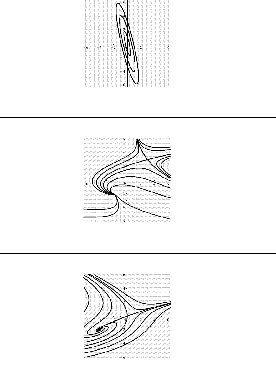
Chapter 12
Figure 12–D: Phase plane diagram in Problem 20, Section 12.2
Figure 12–E: Phase plane diagram in Problem 14, Section 12.3
Figure 12–F: Phase plane diagram in Problem 16, Section 12.3
310
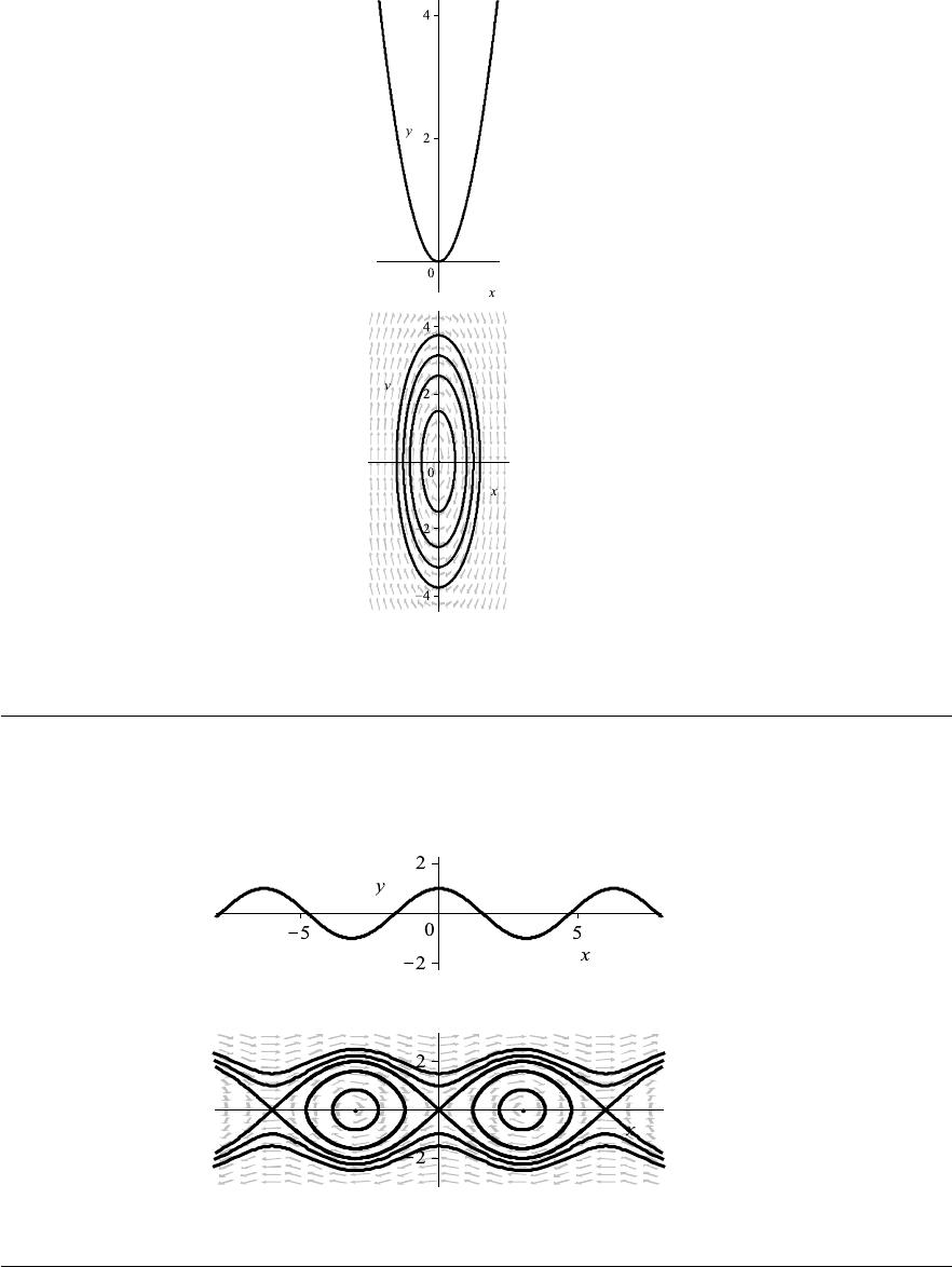
Figures
Figure 12–G: Potential and Phase plane diagrams in Problem 8, Section 12.4
Figure 12–H: Potential and Phase plane diagrams in Problem 10, Section 12.4
311
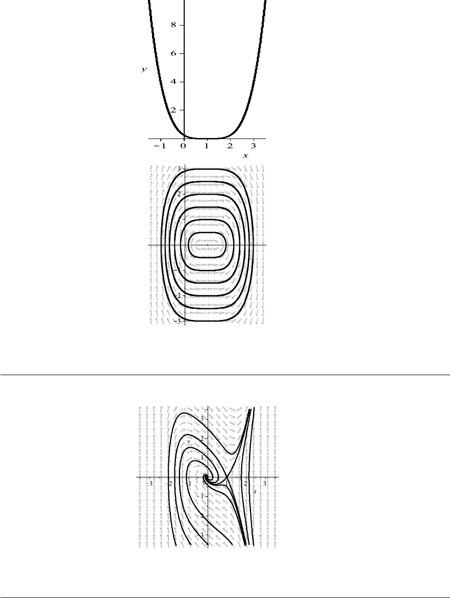
Chapter 12
Figure 12–I: Potential and Phase plane diagrams in Problem 12, Section 12.4
Figure 12–J: Phase plane diagram in Problem 14, Section 12.4
312
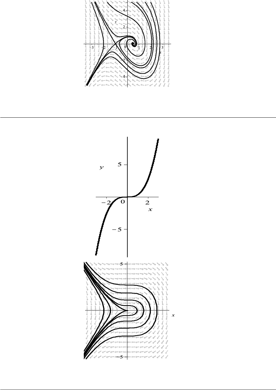
Figures
Figure 12–K: Phase plane diagram in Problem 16, Section 12.4
Figure 12–L: Potential and Phase plane diagrams in Problem 18, Section 12.4
313
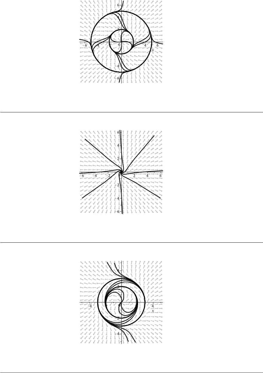
Chapter 12
Figure 12–M: Phase plane diagram in Problem 6, Se ction 12.6
Figure 12–N: Phase plane diagram in Problem 8, Section 12.6
Figure 12–O: Phase plane diagram in Problem 10, Section 12.6
314
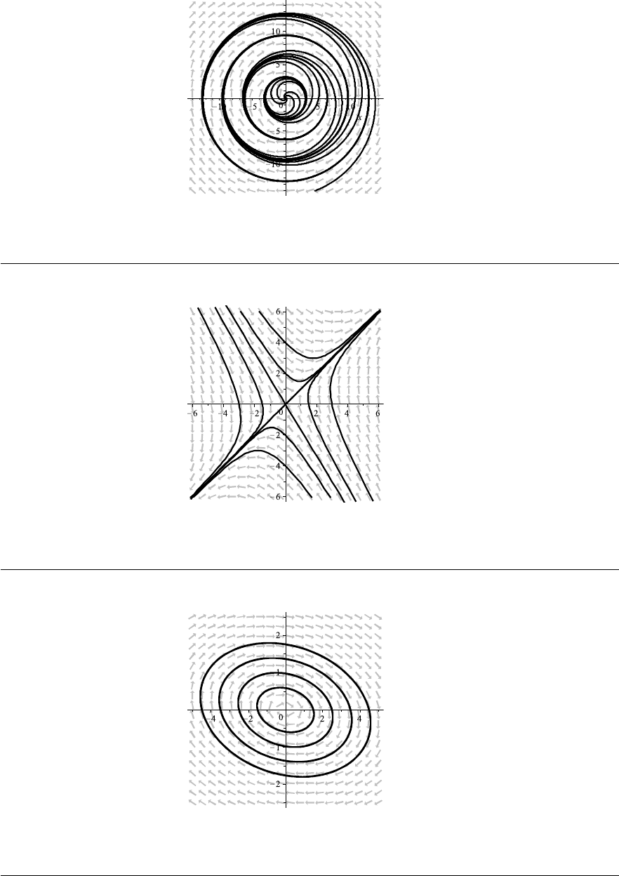
Figures
Figure 12–P: Phase plane diagram in Problem 12, Section 12.6
Figure 12–Q: Phase plane diagram in Problem 2, Review Section
Figure 12–R: Phase plane diagram in Problem 4, Review Section
315
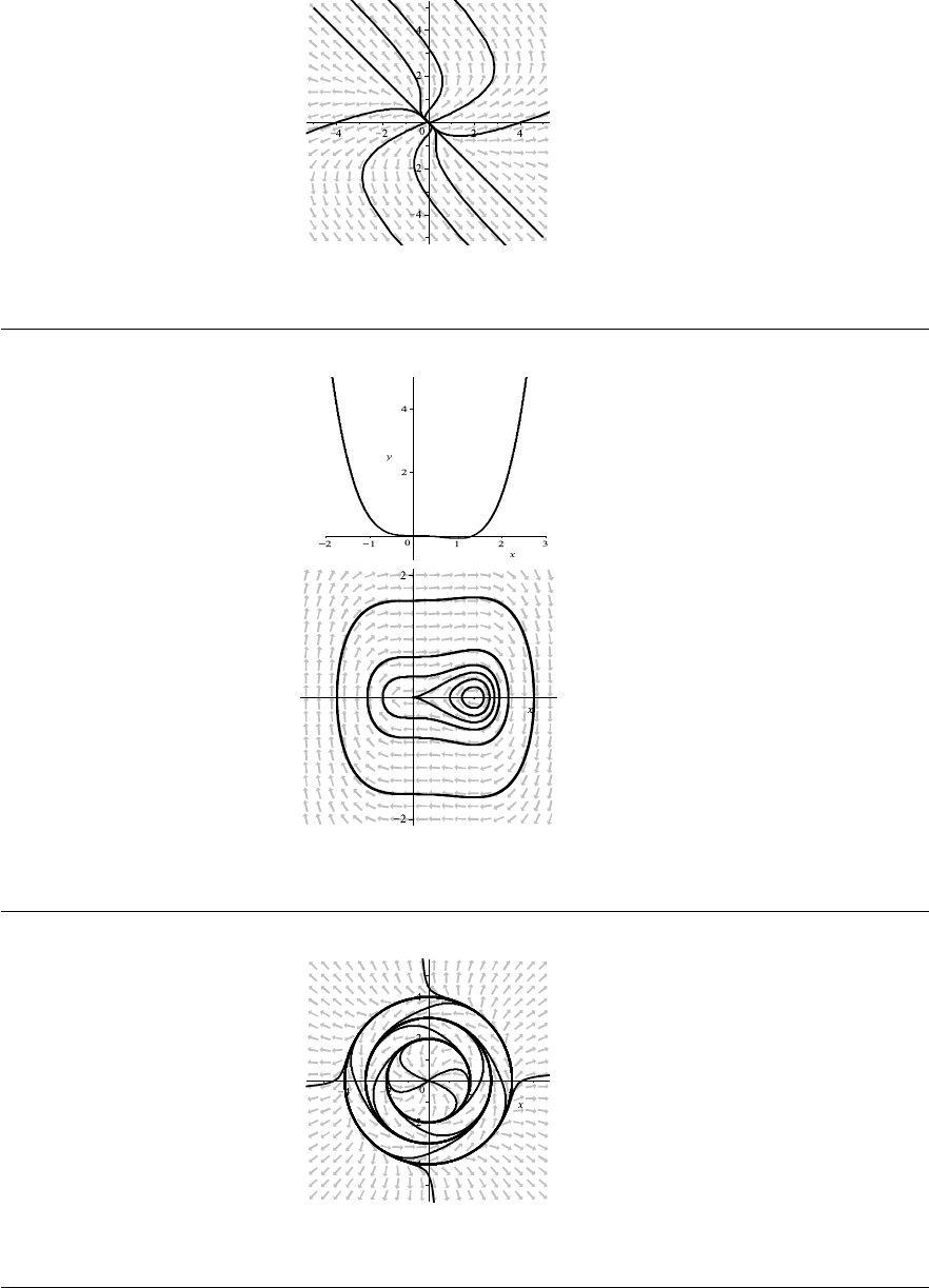
Chapter 12
Figure 12–S: Phase plane diagram in Problem 6, Review Section
Figure 12–T: Potential and Phase plane diagrams in Problem 8, Review Section
Figure 12–U: Phase plane diagram in Problem 14, Review Section
316
CHAPTER 13: Existence and Uniqueness Theory
EXERCISES 13.1: Introduction: Successive Approximations
2. y(x) =
x
R
π
sin[t + y(t)] dt
4. y(x) = 1 +
x
R
0
e
y(t)
dt
6. 0.3775396
8. 2.2360680
10. 1.9345632
12. y
1
(x) = 1 + x; y
2
(x) = 1 + x + x
2
+
1
3
x
3
14. y
1
(x) = y
2
(x) = sin x
16. y
1
(x) =
3
2
− x +
1
2
x
2
;
y
2
(x) =
5
3
−
3
2
x + x
2
−
1
6
x
3
EXERCISES 13.2: Picard’s Existence and Uniqueness Theorem
2. No
4. Ye s
6. Ye s
14. No. Let y
n
(x) =
n
2
x , 0 ≤ x ≤ (1/n)
2n − n
2
x , (1/n) ≤ x ≤ (2/n)
0 , 2/n ≤ x ≤ 1 .
Then
lim
n→∞
y
n
(x) = 0 ,
317

Chapter 13
but
lim
n→∞
1
Z
0
y
n
(x) dx = 1 6= 0 .
EXERCISES 13.3: Existence of Solutions of Linear Equations
2. [−2, 1)
4. (0, 3]
6. (−∞, ∞)
EXERCISES 13.4: Continuous Dependence of Solutions
2. 10
−2
e
4. 10
−2
e
√
2 e
−1/2
6. 10
−2
e
8.
1
24
e
sin 1
10.
e
6
REVIEW PROBLEMS
2. 0.7390851
4. 9 +
x
Z
0
[t
2
y
3
(t) − y
2
(t)] dt
6. y
1
(x) = −1 + 2x; y
2
(x) = −1 + 2x −2x
2
8. No
10.
−
π
2
,
π
2
12.
e
6
318
