Copyright © 2012 Pearson Education, Inc.
O O
O O
O O
O O
O O
(1.1.5)(1.1.5)
(1.1.4)(1.1.4)
(1.1.3)(1.1.3)
O O
(1.1.1)(1.1.1)
(1.1.6)(1.1.6)
(1.1.2)(1.1.2)
O O
3. Demonstrations of Using Maple in Calculus and Differential
Equations
In this second introductory section we will give demonstrations of how Maple can be used in calculus and
differential equations. Later, as you work through some of the lab sections, it may be helpful to return to
this section to see how some of the code in Maple is actually used.
We will begin with some calculus operations that include algebraic manipulations.
3.1 Calculus Examples
The techniques introduced above will now be applied to the fundamental concepts: limit, derivative, and
integral, and their applications.
Limits
restart
The Maple command to compute lim
x / a
f x is limit f x , x = a . A limit template can be entered
in 2D input by typing limit then [esc]/[enter]. Press the [tab] key to move from one position to to
the next.
lim
x / 0
sin x
x
1
lim
x / 0
1 C x
1
x
e
The infinity symbol is entered by typing infinity [esc].
lim
n / N
1 C
x
n
n
e
x
Right- and left-hand limits are returned when a "plus" or a "minus" is entered in the exponent of the
limiting point.
lim
x / 0
ln x
x
undefined
lim
x / 0
C
ln x
x
K
N
lim
x / 0
K
x
x
K
1
Using 1D input, the last limit is calculated like this.
Maple Manual for Fundamentals of Differential Equations, 8e, and Fundamentals of Differential Equations and Boundary Value Problems, 6e.
53
Copyright © 2012 Pearson Education, Inc.
O O
O O
(1.2.2)(1.2.2)
(1.2.4)(1.2.4)
O O
O O
O O
(1.2.5)(1.2.5)
(1.1.8)(1.1.8)
O O
(1.2.3)(1.2.3)
O O
O O
O O
O O
(1.1.9)(1.1.9)
(1.1.7)(1.1.7)
(1.2.1)(1.2.1)
O O
limit( abs(x)/x, x=0, left);
K
1
Limits at infinity can also be handled.
lim
x/C N
arctan x
1
2
!
Here is the 1D input for the arctan limit.
limit( arctan(x), x=+infinity);
1
2
!
Difference Quotients and Derivatives
restart
Given a function f , the slope of the secant line through x, f x and x C h, f x C h is called
the difference quotient. As h approaches 0, these quantities converge to the slope of the tangent line
at x, f x . The slope of the secant line can be obtained with the Maple command
m secant d
f x C h
K
f x
h
m
secant
:=
f x C h
K
f x
h
The difference quotient formula is now stored in table named m.
In practise, it is often necessary to use the simplify command to force Maple to simplify the
difference quotient. For example,
f x d x
3
K
3 x
2
K
4
f := x/x
3
K
3 x
2
K
4
Notice that in the previous command, Maple complains about parts of the expression being
ambiguous, in this case, f x . If you intended this to define a function, select the function definition
from the drop-down box that shows up. You should NOT really use f x to define a function!
m secant
x C h
3
K
3 x C h
2
K
x
3
C 3 x
2
h
simplify m secant
3 x
2
C 3 x h C h
2
K
6 x
K
3 h
m tangent d lim
h / 0
m secant
m
tangent
:= 3 x
2
K
6 x
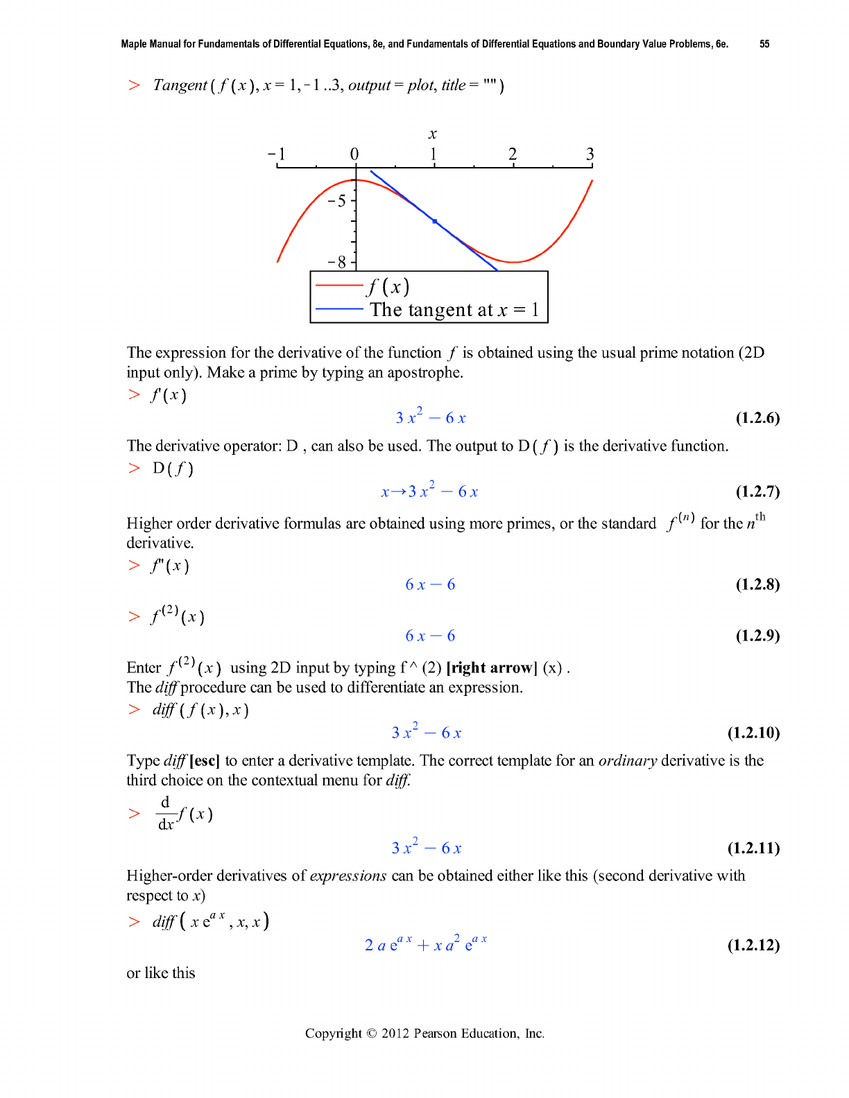
The Tangent command from the Student Calculus1 package provides a simple means to display a
function and the tangent line at a point.
with Student Calculus1 :
The optional equation title = "" is to suppress the (rather long) default title to the plot.
Maple Manual for Fundamentals of Differential Equations, 8e, and Fundamentals of Differential Equations and Boundary Value Problems, 6e.
54
Copyright © 2012 Pearson Education, Inc.
(1.2.21)(1.2.21)
O O
(1.2.13)(1.2.13)
(1.2.14)(1.2.14)
(1.2.18)(1.2.18)
(1.2.19)(1.2.19)
O O
O O
O O
O O
(1.2.20)(1.2.20)
O O
(1.2.17)(1.2.17)
(1.2.15)(1.2.15)
(1.2.16)(1.2.16)
O O
O O
O O
d
2
dx
2
x e
a x
2 a e
a x
C x a
2
e
a x
Using 1D input the second derivative calculation is accomplished with the following entry.
diff( x*exp(a*x), x, x);
2 a e
a x
C x a
2
e
a x
Obtain the fifth-order derivative like this
diff x e
a x
, x$5
5 a
4
e
a x
C x a
5
e
a x
or, using diff [esc], like this
d
5
dx
5
x e
a x
5 a
4
e
a x
C x a
5
e
a x
Implicit differentiation is carried out in the same manner, provided that all functional dependencies
are explicitly given in the equation. Here is an example for the function y x defined implicitly by
the following equation.
eqn d x
K
1
4
= x
2
K
y
2
eqn := x
K
1
4
= x
2
K
y
2
Make the substitution y = y x to indicate that the equation is determining y as a function of x .
ImpEqn d subs y = y x , eqn
ImpEqn := x
K
1
4
= x
2
K
y x
2
Differentiate the implicit equation with respect to x.
d
dx
ImpEqn
4 x
K
1
3
= 2 x
K
2 y x
d
dx
y x
Use the isolate command to isolate the derivative.
isolate %,
d
dx
y x
d
dx
y x =
1
2
K
4 x
K
1
3
C 2 x
y x
The second derivative can be found like this.
y'' =
d
dx
rhs %
d
2
dx
2
y x =
1
2
K
12 x
K
1
2
C 2
y x
K
1
2
K
4 x
K
1
3
C 2 x
d
dx
y x
y x
2
Maple Manual for Fundamentals of Differential Equations, 8e, and Fundamentals of Differential Equations and Boundary Value Problems, 6e.
56
Copyright © 2012 Pearson Education, Inc.
(1.3.1.1)(1.3.1.1)
(1.2.23)(1.2.23)
(1.2.24)(1.2.24)
O O
O O
O O
O O
O O
O O
(1.2.25)(1.2.25)
O O
O O
(1.2.26)(1.2.26)
(1.2.22)(1.2.22)
Prime notation in Maple (2D input)
One prime on a free variable is interpreted by Maple as the derivative
with respect to x. Two primes is the second derivative.
y' , y''
d
dx
y x ,
d
2
dx
2
y x
Differentiation with respect to the t variable is indicated with a dot
over the variable (Newton's notation). The dot is entered as a period.
y
.
, y
..
d
dt
y t ,
d
2
dt
2
y t
Overdot templates will be found on the Accents palette or, using the
keyboard, by typing y [Control]-["] (this is [Control]-[shift]-['])
and then pressing the period key. Right-arrow your way back to the
baseline. As usual, use the Command key on a Macintosh.
Of course, with Maple at our disposal, it is just as easy to obtain explicit derivative formulas. We
can solve the original equation for y.
soln d solve eqn, y
soln :=
K
1
K
x
4
C 4 x
3
K
5 x
2
C 4 x ,
K
K
1
K
x
4
C 4 x
3
K
5 x
2
C 4 x
Apply the diff procedure to the first solution.
d
dx
soln 1
1
2
K
4 x
3
C 12 x
2
K
10 x C 4
K
1
K
x
4
C 4 x
3
K
5 x
2
C 4 x
And here is the explicit second derivative of the second function defined by eqn. The simplify
procedure is applied to the output to get it into one term.
d
2
dx
2
soln 2 : simplify %
K
2 x
6
K
12 x
5
C 27 x
4
K
36 x
3
C 30 x
2
C 1
K
12 x
K
1
K
x
4
C 4 x
3
K
5 x
2
C 4 x
3 / 2
Applications of Derivatives
Linearization of a Function
restart
The linearization of a function f x at x=a is the function L x = f a C f' a $ x
K
a . To
create this function in Maple we enter
L x d f a C f' a $ x
K
a
L := x/f a C D f a x
K
a
Maple Manual for Fundamentals of Differential Equations, 8e, and Fundamentals of Differential Equations and Boundary Value Problems, 6e.
57
Copyright © 2012 Pearson Education, Inc.
(1.3.1.2)(1.3.1.2)
(1.3.1.3)(1.3.1.3)
O O
O O
(1.3.1.4)(1.3.1.4)
O O
O O
O O
O O
Now, if we want the linearization formula for
f x d 1 C x
f := x/ 1 C x
at
a d 0
a := 0
we need only evaluate L.
L x
1 C
1
2
x
If the function and/or the point are changed
f x d x sin x : a d
5
2
:
then L still provides the correct linearization.
L x ;
plot f x , L x , x = 1 ..4, color = black, linestyle = 1, 3
5
2
sin
5
2
C sin
5
2
C
5
2
cos
5
2
x
K
5
2
x
2 3 4
K
3
K
1
1
3
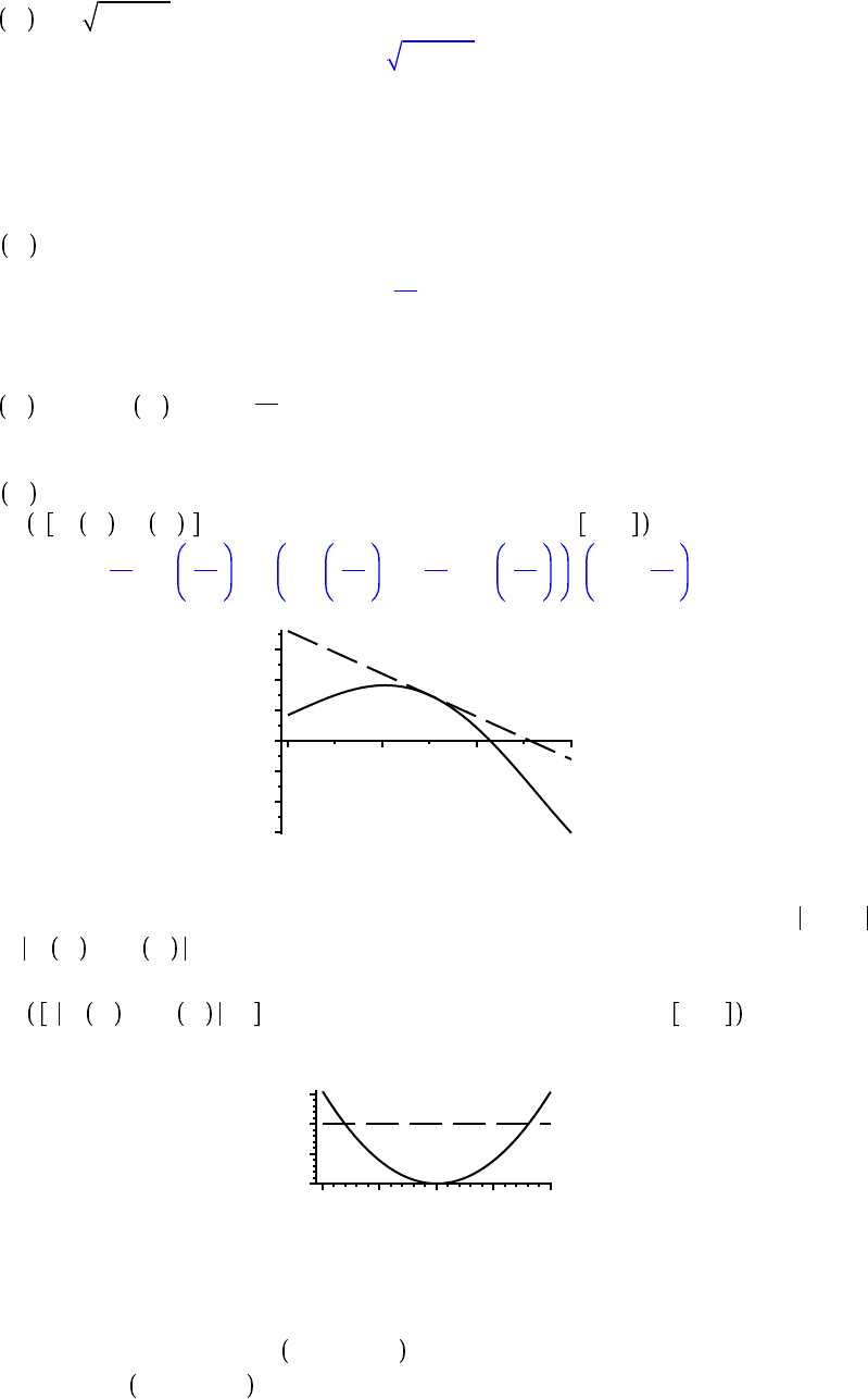
To determine the largest interval on which the linearization displayed above differs from the
function by no more than a specified amount, i.e., to estimate the largest " such that x
K
a ! "
implies f x
K
L x ! e , we first look at the graph.
e d 0.01;
plot f x
K
L x , e , x = 2.4 ..2.6, color = black, linestyle = 1, 3
e := 0.01
x
2.45 2.50 2.55 2.60
0
0.010
Click the left mouse button as close as possible to the leftmost of the two intersections of the
curves in the plot. The box at the left end of the Context Bar shows the approximate coordinates
of this point; this gives the point 2.42, 0.01 . Repeating this process for the rightmost
intersection gives 2.58, 0.01 . This gives the estimate " = 0.08.
More accurate estimates of the intersection points will give more accurate estimates of ". In this
Maple Manual for Fundamentals of Differential Equations, 8e, and Fundamentals of Differential Equations and Boundary Value Problems, 6e.
58
Copyright © 2012 Pearson Education, Inc.
(1.3.2.3)(1.3.2.3)
(1.3.2.2)(1.3.2.2)
O O
O O
O O
O O
(1.3.2.4)(1.3.2.4)
(1.3.2.1)(1.3.2.1)
O O
O O
O O
(1.3.1.5)(1.3.1.5)
O O
O O
(1.3.1.6)(1.3.1.6)
O O
case, Maple can find better approximations.
leftpoint d fsolve f x
K
L x = e, x = 2 ..2.5 ;
rightpoint d fsolve f x
K
L x = e, x = 2.5 ..3
leftpoint := 2.419697538
rightpoint := 2.580447088
This yields
" d min 2.5
K
leftpoint, rightpoint
K
2.5
" := 0.080302462
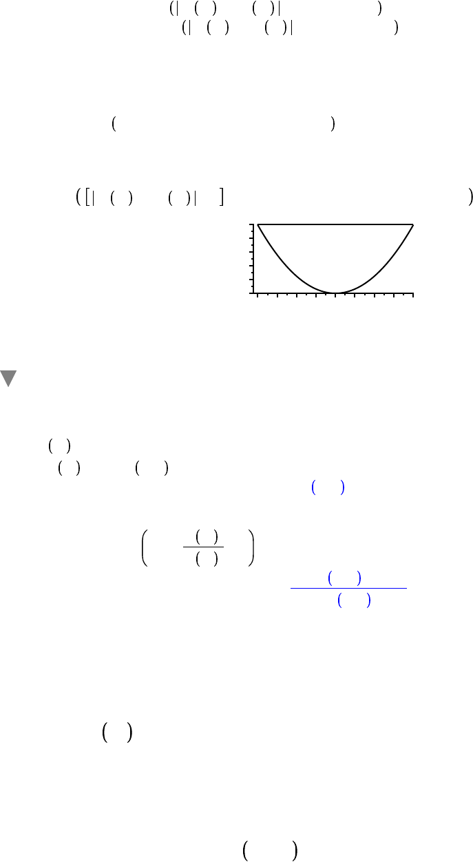
To conclude, check that the error never exceeds e over this interval.
plot f x
K
L x , e , x = 2.5
K
" ..2.5 C ", color = black
x
2.46 2.50 2.54 2.58
0
0.006
0.010
Newton's Method
restart
Newton's Method can be implemented in Maple to find an approximation to the smallest solution
to f x = 0 with
f x d cos 5 x
K
x
f := x/cos 5 x
K
x
to five decimal places by defining the auxiliary function
g d unapply x
K
f x
f' x
, x
g := x/x
K
cos 5 x
K
x
K
5 sin 5 x
K
1
and an initial guess (use a graph, if necessary, to obtain a starting value)
x
0
d
K
1.0
x
0
:=
K
1.0
The next approximation is
x
1
d g x
0
x
1
:=
K
0.7784735010
Note that we are using a table named x to store the approximate solutions.
Continuing in the same manner we can use a simple for..do loop to calculate three more
approximations.
for n from 2 to 4 do x
n
d g x
n
K
1
end do
x
2
:=
K
0.7677474241
Maple Manual for Fundamentals of Differential Equations, 8e, and Fundamentals of Differential Equations and Boundary Value Problems, 6e.
59
Copyright © 2012 Pearson Education, Inc.
(1.3.3.1)(1.3.3.1)
(1.3.2.5)(1.3.2.5)
O O
(1.3.3.3)(1.3.3.3)
(1.3.2.6)(1.3.2.6)
(1.3.3.4)(1.3.3.4)
O O
O O
(1.3.3.5)(1.3.3.5)
O O
O O
(1.3.3.6)(1.3.3.6)
O O
O O
O O
O O
O O
(1.3.3.2)(1.3.3.2)
x
3
:=
K
0.7674935683
x
4
:=
K
0.7674934212
Thus, x = 0.767493 appears to be a 6-digit approximation for the smallest root. If this process
had continued too much longer, it would be efficient to use the following modification of the
loop.
for n from 2 while x
n
K
1
K
x
n
K
2
R 10
K
6
do x
n
d g x
n
K
1
; end do
x
2
:=
K
0.7677474241
x
3
:=
K
0.7674935683
x
4
:=
K
0.7674934212
Maxima-Minima
Consider the following sequence of operations relating to the function
x t = e
K
#t
cos $ t C % . What information is obtained in each step?
restart;
x d exp
K
alpha$t $cos omega$t C theta ;
# Note that x is not declared to be a function but is an expression. We will refer to it
as x below instead of x(t).
x := e
K
# t
cos $ t C %
dx d diff x, t ;
dx :=
K
# e
K
# t
cos $ t C %
K
e
K
# t
sin $ t C % $
dx2 d diff x, t$2 ;
dx2 := #
2
e
K
# t
cos $ t C % C 2 # e
K
# t
sin $ t C % $
K
e
K
# t
cos $ t C % $
2
factor dx ;
K
e
K
# t
# cos $ t C % C sin $ t C % $
CriticalPoint d solve dx = 0, t ;
CriticalPoint :=
K
% C arctan
#
$
$
subs( t=CriticalPoint, dx2 );
#
2
e
# % C arctan
#
$
$
cos
K
arctan
#
$
C 2 # e
# % C arctan
#
$
$
sin
K
arctan
#
$
$
K
e
# % C arctan
#
$
$
cos
K
arctan
#
$
$
2
dx2:=simplify( (1.3.3.6),trig);#We have used the equation labels on the right.
Maple Manual for Fundamentals of Differential Equations, 8e, and Fundamentals of Differential Equations and Boundary Value Problems, 6e.
60
Copyright © 2012 Pearson Education, Inc.
O O
(1.3.3.9)(1.3.3.9)
O O
O O
(1.3.3.8)(1.3.3.8)
O O
(1.3.3.10)(1.3.3.10)
O O
(1.3.3.7)(1.3.3.7)
(1.4.1)(1.4.1)
O O
O O
(1.3.3.11)(1.3.3.11)
dx2 :=
K
#
2
e
# % C arctan
#
$
$
#
2
$
2
C 1
K
e
# % C arctan
#
$
$
$
2
#
2
$
2
C 1
Since the second derivative at the critical point will be negative (for real values of omega, alpha,
and theta), this critical point must be a (local) maximum. The value of the function at this
maximum is
X max d simplify subs t = CriticalPoint, x , trig ;
X
max
:=
e
# % C arctan
#
$
$
#
2
$
2
C 1
Note the effect of [max] on the symbol X. It becomes a subscript. It is important to realize that
the symbol X (upper-case) is not the same as the symbol x (lower case). The disastrous effect
can be observed by changing the symbol above into lower case letters and re-executing the
command and the next two commands below. Indefinite and definite integration is obtained in a
natural way:
Int x, t ;
e
K
# t
cos $ t C % dt
simplify value (1.3.3.9) ;
K
e
K
# t
# cos $ t C %
K
sin $ t C % $
#
2
C $
2
Note that the constant of integration is not included in the result. One can use the symbol palette
to input the commands:
simplify x dt ;
K
e
K
# t
# cos $ t C %
K
sin $ t C % $
#
2
C $
2
Definite, Indefinite, and Improper Integrals
restart
The int procedure is used to compute integrals in Maple. The syntax of an indefinite integral is
int f x , x .
int ln x , x
Maple Manual for Fundamentals of Differential Equations, 8e, and Fundamentals of Differential Equations and Boundary Value Problems, 6e.
61
Copyright © 2012 Pearson Education, Inc.
(1.4.4)(1.4.4)
O O
O O
(1.4.5)(1.4.5)
(1.4.3)(1.4.3)
(1.4.7)(1.4.7)
O O
(1.4.8)(1.4.8)
O O
O O
(1.4.6)(1.4.6)
(1.4.1)(1.4.1)
O O
O O
O O
O O
O O
(1.4.2)(1.4.2)
(1.4.9)(1.4.9)
x ln x
K
x
Note that Maple does not add an arbitrary constant.
A definite integral over the interval a, b is evaluated with the entry int f x , x = a ..b .
int ln x , x = 1 ..4
K
3 C 8 ln 2
Both these integrals can also be entered from the Expression palette. Alternatively, type int [esc] to
obtain a contextual menu with even more integral templates.
x sin x dx
sin x
K
x cos x
0
6
x sin x dx
sin 6
K
6 cos 6
If approximate (decimal) limits are used, Maple evaluates the integral numerically.
0
6.0
x sin x dx
K
6.040437218
We will use Maple to find the function that satisfies the initial value problem y' = 5 e
K
3 x
,
y 0 =
K
10. This problem can actually be solved in two ways.
Method 1. First find an antiderivative, including an arbitrary constant.
eq1 d y = 5 e
K
3 x
dx C C
eq1 := y =
K
5
3
e
K
3 x
C C
Apply the initial condition to determine the appropriate value of C.
eq2 d subs x = 0, y =
K
10, eq1
eq2 :=
K
10 =
K
5
3
e
0
C C
Solve for C.
isolate eq2, C
C =
K
25
3
Substitute this value into eq1.
subs (1.4.8), eq1
y =
K
5
3
e
K
3 x
K
25
3
Method 2. Use a definite integral with lower limit 0 and upper limit x as the antiderivative. Add the
initial value of y as the constant of integration.
Note the use of the dummy integration variable & instead of x. (& is Greek for x . Enter it by typing
Maple Manual for Fundamentals of Differential Equations, 8e, and Fundamentals of Differential Equations and Boundary Value Problems, 6e.
62
Copyright © 2012 Pearson Education, Inc.
(1.4.15)(1.4.15)
O O
(1.4.19)(1.4.19)
O O
(1.4.14)(1.4.14)
(1.4.20)(1.4.20)
O O
(1.4.13)(1.4.13)
(1.4.17)(1.4.17)
O O
O O
(1.4.16)(1.4.16)
O O
O O
(1.4.18)(1.4.18)
O O
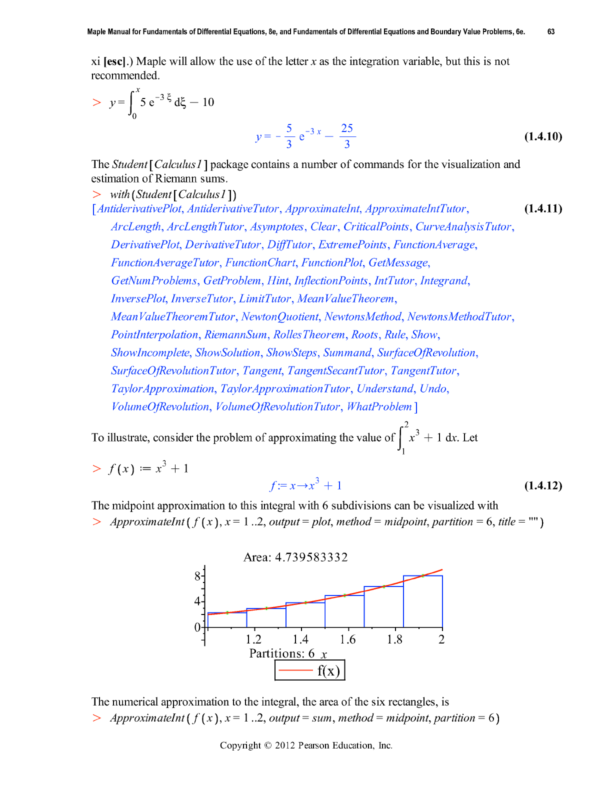
1
6
>
i = 0
5
13
12
C
1
6
i
3
C 1
evalf %
4.739583334
For right-hand sums use method = right and for left-hand sums, method = left. For the Trapezoidal
and Simpson's Rules, use trapzoid and simpson respectively. For example,
evalf ApproximateInt f x , x = 1 ..2, output = sum, method = trapezoid, partition = 6
4.770833333
The exact value of the definite integral is
1
2
f x dx; evalf %
19
4
4.750000000
While Maple is designed to be able to automatically evaluate many integrals, it can also be used to
assist with techniques such as substitution and integration by parts. To prevent Maple from
evaluating an integral, definite or indefinite, use Int, the inert form of int. The value command is
used to force the symbolic evaluation of an inert command. A substitution is carried out with the
dchange command in the PDETools package. The next entry defines an inert integral and names it
R.
R d
0
3
x 3 x C 1 dx
R :=
0
3
x 3 x C 1 dx
Load the PDETools package (suppress output).
with PDETools :
Define a change-of-variable equation and use isolate to generate the inverse change-of-variable
equation.
cv d u = 3 x C 1;
icv d isolate cv, x
cv := u = 3 x C 1
icv := x =
1
3
u
K
1
3
Apply dchange to the sequence icv, R .
dchange icv, R
1
10
1
3
1
3
u
K
1
3
u du
simplify %
Maple Manual for Fundamentals of Differential Equations, 8e, and Fundamentals of Differential Equations and Boundary Value Problems, 6e.
64
Copyright © 2012 Pearson Education, Inc.
(1.4.23)(1.4.23)
(1.4.21)(1.4.21)
O O
(1.4.20)(1.4.20)
O O
(1.4.22)(1.4.22)
O O
(1.4.24)(1.4.24)
O O
O O
1
9
1
10
u
K
1 u du
value %
100
27
10 C
4
135
To check the answer, compare it to the Maple-generated value of the original integral.
value R
100
27
10 C
4
135
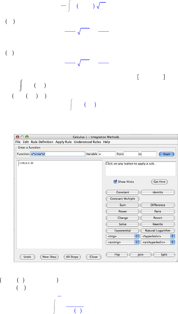
Integration-by-parts can be applied using the IntTutor in the Student Calculus1 package. To apply
it to the integral x sin a x dx, evaluate the entry
IntTutor x sin a x , x
x sin a x dx
Doing so produces the following dialogue allowing for the application of any one of a number of
integration techniques.
Here's an example taken from the CRC Tables of Integrals.
Int u / sin u , u = 0 ..Pi/ 2 :
% = value % ;
0
1
2
!
u
sin u
du = 2 Catalan
Maple Manual for Fundamentals of Differential Equations, 8e, and Fundamentals of Differential Equations and Boundary Value Problems, 6e.
65
Copyright © 2012 Pearson Education, Inc.
(1.5.1.5)(1.5.1.5)
O O
O O
(1.5.1.1)(1.5.1.1)
O O
O O
(1.5.1.7)(1.5.1.7)
(1.5.1.6)(1.5.1.6)
O O
O O
(1.5.1.2)(1.5.1.2)
O O
O O
O O
(1.5.1.3)(1.5.1.3)
O O
(1.4.25)(1.4.25)
(1.5.1.4)(1.5.1.4)
O O
evalf rhs % ;
1.831931188
Applications of Integrals
Arclength of a Smooth Curve
restart
The definite integral for the arclength of a smooth curve is usually easy to setup but difficult to
evaluate.
f d
4
2
3
$x
3
2
K
1
f :=
4
3
2 x
3 / 2
K
1
0
1
1 C
d
dx
f
2
dx
13
6
Or, if the curve is entered in Maple as a function
f x d
4
2
3
$x
3
2
K
1
f := x/
4
3
2 x
3 / 2
K
1
0
1
1 C f' x
2
dx
13
6
Maple is able to evaluate many more integrals than most humans, but there are many arclength
integrals that cannot be evaluated explicitly. If this occurs, or if Maple's answer involves
functions that are not familiar to you, use evalf to force a numerical approximation of the integral.
f x d sin x
f := x/sin x
0
1
1 C f' x
2
dx
2 EllipticE 1
K
cos 1
2
,
1
2
2
evalf %
1.311442498
Maple Manual for Fundamentals of Differential Equations, 8e, and Fundamentals of Differential Equations and Boundary Value Problems, 6e.
66
Copyright © 2012 Pearson Education, Inc.
(1.5.2.4)(1.5.2.4)
(1.5.2.3)(1.5.2.3)
(1.5.2.5)(1.5.2.5)
(1.5.2.6)(1.5.2.6)
O O
O O
O O
O O
O O
O O
(1.5.2.1)(1.5.2.1)
O O
O O
(1.5.2.2)(1.5.2.2)
O O
(1.5.2.7)(1.5.2.7)
O O
O O
O O
Improper Integrals
restart
Improper integrals are no problem for Maple. Here are three examples.
1
N
x e
K
x
dx
2 e
K
1
0
2
1
4
K
x
2
dx
1
2
!
1
N
1
x
dx
N
int exp
K
u
2
, u = 0 ..infinity ;
1
2
!
int exp
K
a$u
2
, u = 0 ..infinity ;
lim
u/N
1
2
! erf a u
a
Note that Maple is unable to evaluate this limit until something is known about the parameter a.
about a ;
a:
nothing known about this object
assume a O 0 ;
about a ;
Originally a, renamed a~:
is assumed to be: RealRange(Open(0),infinity)
int exp
K
a$u
2
, u = 0 ..infinity ;
1
2
!
a~
We can remove the assumption on a by assigning the symbol to itself.
a d'a';
a := a
about a ;
a:
nothing known about this object
Maple Manual for Fundamentals of Differential Equations, 8e, and Fundamentals of Differential Equations and Boundary Value Problems, 6e.
67
Copyright © 2012 Pearson Education, Inc.
O O
O O
O O
(1.5.3.5)(1.5.3.5)
(1.5.3.3)(1.5.3.3)
(1.5.3.2)(1.5.3.2)
O O
O O
(1.5.3.4)(1.5.3.4)
(1.5.3.6)(1.5.3.6)
O O
O O
(1.5.3.1)(1.5.3.1)
Integration of a Rational Function
Consider the proper rational function:
f d
x
2
K
26$ x
K
47
x
5
C 5$ x
3
C 3$ x
4
C 11$ x
2
K
20
;
f :=
x
2
K
26 x
K
47
x
5
C 5 x
3
C 3 x
4
C 11 x
2
K
20
The antiderivative of f can be obtained by a variety of different means. Let's examine a few and
compare the information obtained in each case.
F d Int f, x ;
F :=
x
2
K
26 x
K
47
x
5
C 5 x
3
C 3 x
4
C 11 x
2
K
20
dx
The simplest, but least instructive, approach is to simply let Maple do all the work. Note that
the constant of integration is not included in indefinite integrals.
F = value F ;
x
2
K
26 x
K
47
x
5
C 5 x
3
C 3 x
4
C 11 x
2
K
20
dx =
23
27
ln x C 2
K
4
3
ln x
K
1
C
13
54
ln x
2
C 5 C
91
135
5 arctan
1
5
x 5 C
1
3 x C 2
or alternatively,
int f, x ;
23
27
ln x C 2
K
4
3
ln x
K
1 C
13
54
ln x
2
C 5 C
91
135
5 arctan
1
5
x 5
C
1
3 x C 2
To emphasize integration techniques while still avoiding algebraic complications, we can utilize
Maple to determine the partial fraction expansion of the integrand.
fpf d convert f, parfrac, x ;
fpf :=
1
27
13 x C 91
x
2
C 5
K
1
3 x C 2
2
K
4
3 x
K
1
C
23
27 x C 2
From this partial fraction decomposition it is now a relatively simple matter to compute the
integral BY HAND. The result can be compared with the previous answer. But let Maple do it.
int fpf, x ;
23
27
ln x C 2
K
4
3
ln x
K
1 C
13
54
ln x
2
C 5 C
91
135
5 arctan
1
5
x 5
Maple Manual for Fundamentals of Differential Equations, 8e, and Fundamentals of Differential Equations and Boundary Value Problems, 6e.
68
Copyright © 2012 Pearson Education, Inc.
(1.5.3.11)(1.5.3.11)
(1.5.3.12)(1.5.3.12)
O O
(1.5.3.13)(1.5.3.13)
O O
O O
O O
(1.5.3.8)(1.5.3.8)
O O
(1.5.3.7)(1.5.3.7)
O O
O O
(1.5.3.9)(1.5.3.9)
(1.5.3.10)(1.5.3.10)
C
1
3 x C 2
The third and final approach to this problem will be the most detailed. The purpose here is to
emphasize the process of finding a partial fraction expansion without fear of unmanageable
algebra. The key here is to enter the correct form for the partial fraction decomposition. This
form depends upon the irreducible factors in the denominator of f.
factor denom f ;
x
K
1 x
2
C 5 x C 2
2
The appropriate general form for the decomposition will be
FORM d
a
x
K
1
C
b
x C 2
C
c
x C 2
2
C
d C e$x
x
2
C 5
;
FORM :=
a
x
K
1
C
b
x C 2
C
c
x C 2
2
C
d C e x
x
2
C 5
The second step is to determine the (linear) equations that define the constants a, b, c, d, and e.
eqn d f = FORM;
eqn :=
x
2
K
26 x
K
47
x
5
C 5 x
3
C 3 x
4
C 11 x
2
K
20
=
a
x
K
1
C
b
x C 2
C
c
x C 2
2
C
d C e x
x
2
C 5
simplify eqn$denom f ;
x
2
K
26 x
K
47 = a x
4
C 4 a x
3
C 9 a x
2
C 20 a x C 20 a C b x
4
C b x
3
C 3 b x
2
C 5 b x
K
10 b C c x
3
K
c x
2
C 5 c x
K
5 c C d x
3
C 3 d x
2
K
4 d C e x
4
C 3 e x
3
K
4 e x
This equation is true for all x. We can collect common powers of x to identify the coefficients.
collect (1.5.3.10), x ;
x
2
K
26 x
K
47 = a C e C b x
4
C 4 a C 3 e C c C d C b x
3
C 9 a C 3 b
K
c
C 3 d x
2
C
K
4 e C 5 b C 5 c C 20 a x
K
5 c
K
10 b
K
4 d C 20 a
eqns d coeffs rhs (1.5.3.11) , x ;
eqns :=
K
5 c
K
10 b
K
4 d C 20 a,
K
4 e C 5 b C 5 c C 20 a, 9 a C 3 b
K
c
C 3 d, 4 a C 3 e C c C d C b, a C e C b
Notice that the coefficients are not necessarily ordered in increasing powers of x. We obtain the
following system of 5 linear equations in 5 unknowns.
systemofequations d eqns 1 =
K
47, eqns 2 =
K
26, eqns 3 = 1, eqns 4 = 0,
eqns 5 = 0 ;
systemofequations := a C e C b = 0, 9 a C 3 b
K
c C 3 d = 1,
K
5 c
K
10 b
K
4 d
Maple Manual for Fundamentals of Differential Equations, 8e, and Fundamentals of Differential Equations and Boundary Value Problems, 6e.
69
Copyright © 2012 Pearson Education, Inc.
(1.5.4.2)(1.5.4.2)
• •
(1.5.3.15)(1.5.3.15)
O O
O O
(1.5.3.16)(1.5.3.16)
O O
O O
• •
O O
O O
(1.5.4.1)(1.5.4.1)
O O
(1.5.3.14)(1.5.3.14)
C 20 a =
K
47,
K
4 e C 5 b C 5 c C 20 a =
K
26, 4 a C 3 e C c C d C b = 0
The solution to these equations is
COEFFS d solve systemofequations, a, b, c, d, e ;
COEFFS := a =
K
4
3
, b =
23
27
, c =
K
1
3
, d =
91
27
, e =
13
27
Substituting this result, which is a set, into the original form for the partial fraction
decomposition yields
subs COEFFS, FORM ;
K
4
3 x
K
1
C
23
27 x C 2
K
1
3 x C 2
2
C
13
27
x C
91
27
x
2
C 5
This agrees with (1.5.3.5). The integral is now much simpler to evaluate by hand, but here it is
one last time according to Maple.
int (1.5.3.15), x ;
23
27
ln x C 2
K
4
3
ln x
K
1 C
13
54
ln x
2
C 5 C
91
135
5 arctan
1
5
x 5
C
1
3 x C 2
Note that this same outline can be used on ANY partial fraction problem. The key steps are
knowing the correct form for the partial fraction decomposition and
understanding how to identify the conditions that the coefficients must satisfy.
These are (relatively) high level concepts; the user is relieved of the rather complicated
mechanical manipulations.
Multiple Integrals
restart
The int and Int commands can be used to construct iterated integrals corresponding to double
and triple integrals.
Int Int exp x
K
y , x = y ..1 , y = 0 ..1 ;
value %
0
1
y
1
e
x
K
y
dx dy
e
K
2
Using single integral templates, one inside the other, this integral calculation looks like this (2D
input only).
0
1
y
1
e
x
K
y
dx dy
Maple Manual for Fundamentals of Differential Equations, 8e, and Fundamentals of Differential Equations and Boundary Value Problems, 6e.
70
Copyright © 2012 Pearson Education, Inc.
O O
(1.5.4.2)(1.5.4.2)
• •
O O
• •
• •
• •
O O
(2.1)(2.1)
(2.2)(2.2)
• •
• •
• •
(1.5.4.3)(1.5.4.3)
O O
O O
e
K
2
The area inside of the ellipse
x
2
a
2
C
y
2
b
2
= 1 can be found by parametrizing the ellipse in polar
coordinates: x = a r cos % , y = b r sin % with 0 % r % 1 and 0 % % % 2 !. The Jacobian
of this change-of-variables is a$b$r, so the area of the ellipse is
0
2 !
0
1
a$b$r dr d%
a b !
Note that this result reduces to the familiar area of a circle when a = b.
3.2 Differential Equations Demonstrations
In this section we will demonstrate the use of Maple in working with differential equations. The
following topics are covered in the following subsections.
Direction Fields and Graphical Solutions (Sections 1.3 and 5.4 of Nagle/Saff/Snider)
Symbolic Solutions to Second Order Ordinary Differential Equations and Initial-Value Problems
(Chapter 4 of Nagle/Saff/Snider)
Expressions and Functions (Chapter 4 of Nagle/Saff/Snider)
Systems of Ordinary Differential Equations (Sections 5.2, 5.4 and 5.5 of Nagle/Saff/Snider)
Numeric Solutions (Sections 3.6 and 5.3 of Nagle/Saff/Snider)
Series Solutions (Chapter 8 of Nagle/Saff/Snider)
Laplace Transforms (Chapter 7 of Nagle/Saff/Snider)
It is a good habit to remember to use restart when starting a new problem.
restart;
Another good habit is to load the plots and DEtools packages at the top of all worksheets, just in case
they will be needed at some point in the analysis.
with plots ;
animate, animate3d, animatecurve, arrow, changecoords, complexplot, complexplot3d,
conformal, conformal3d, contourplot, contourplot3d, coordplot, coordplot3d, densityplot,
display, dualaxisplot, fieldplot, fieldplot3d, gradplot, gradplot3d, implicitplot,
implicitplot3d, inequal, interactive, interactiveparams, intersectplot, listcontplot,
listcontplot3d, listdensityplot, listplot, listplot3d, loglogplot, logplot, matrixplot, multiple,
odeplot, pareto, plotcompare, pointplot, pointplot3d, polarplot, polygonplot,
polygonplot3d, polyhedra_supported, polyhedraplot, rootlocus, semilogplot, setcolors,
setoptions, setoptions3d, spacecurve, sparsematrixplot, surfdata, textplot, textplot3d,
tubeplot
with DEtools ;
Maple Manual for Fundamentals of Differential Equations, 8e, and Fundamentals of Differential Equations and Boundary Value Problems, 6e.
71
Copyright © 2012 Pearson Education, Inc.
(2.1.1)(2.1.1)
O O
(2.2)(2.2)AreSimilar, DEnormal, DEplot, DEplot3d, DEplot_polygon, DFactor, DFactorLCLM,
DFactorsols, Dchangevar, FunctionDecomposition, GCRD, Gosper, Heunsols,
Homomorphisms, IVPsol, IsHyperexponential, LCLM, MeijerGsols,
MultiplicativeDecomposition, ODEInvariants, PDEchangecoords,
PolynomialNormalForm, RationalCanonicalForm, ReduceHyperexp, RiemannPsols,
Xchange, Xcommutator, Xgauge, Zeilberger, abelsol, adjoint, autonomous, bernoullisol,
buildsol, buildsym, canoni, caseplot, casesplit, checkrank, chinisol, clairautsol,
constcoeffsols, convertAlg, convertsys, dalembertsol, dcoeffs, de2diffop, dfieldplot,
diff_table, diffop2de, dperiodic_sols, dpolyform, dsubs, eigenring,
endomorphism_charpoly, equinv, eta_k, eulersols, exactsol, expsols, exterior_power,
firint, firtest, formal_sol, gen_exp, generate_ic, genhomosol, gensys, hamilton_eqs,
hypergeomsols, hyperode, indicialeq, infgen, initialdata, integrate_sols, intfactor,
invariants, kovacicsols, leftdivision, liesol, line_int, linearsol, matrixDE, matrix_riccati,
maxdimsystems, moser_reduce, muchange, mult, mutest, newton_polygon, normalG2,
ode_int_y, ode_y1, odeadvisor, odepde, parametricsol, particularsol, phaseportrait,
poincare, polysols, power_equivalent, rational_equivalent, ratsols, redode, reduceOrder,
reduce_order, regular_parts, regularsp, remove_RootOf, riccati_system, riccatisol,
rifread, rifsimp, rightdivision, rtaylor, separablesol, singularities, solve_group,
super_reduce, symgen, symmetric_power, symmetric_product, symtest, transinv,
translate, untranslate, varparam, zoom
Direction Fields and Graphical Solutions (Sections 1.3 and 5.4 of
Nagle/Saff/Snider)
Many introductory courses begin by trying to develop the student's understanding of what a
differential equation is, what it means for a function to solve an ODE, and how to perform some
analysis directly from the differential equation. Graphical methods are commonly employed in these
discussions. The Maple command DEplot, from the DEtools package, provides a comprehensive
interface for most graphical needs.
To begin, consider the first order (linear) differential equation
ODE d diff y x , x = x
2
K
y x ;
ODE :=
d
dx
y x = x
2
K
y x
Note that this is the first example used in Section 1.3 of Nagle/Saff/Snider. The next few commands
reproduce a few of the figures displayed on p.16-18.
The first three arguments to DEplot must provide, in order, a single n-th order ODE or a system of
n first-order ODEs, a dependent variable or a list or set of dependent variables, and a range for the
independent variable. The specific content of the plot is determined by all subsequent arguments to
DEplot.
Maple Manual for Fundamentals of Differential Equations, 8e, and Fundamentals of Differential Equations and Boundary Value Problems, 6e.
72
Copyright © 2012 Pearson Education, Inc.
O O
O O
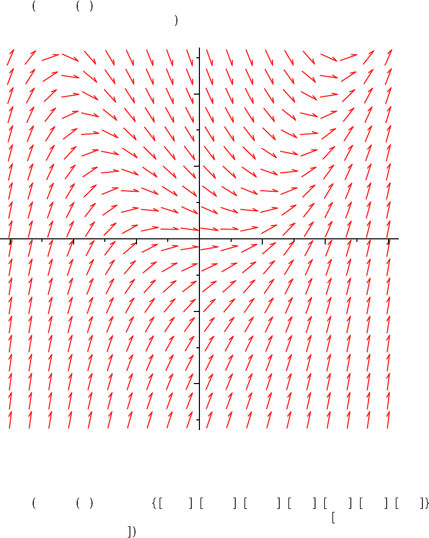
The most basic use of DEplot is to display a direction field for a differential equation. A request for
a direction field is made by specifying both a range for the independent variable and the arrows =
option.
DEplot ODE, y x , x =
K
3 ..3, y =
K
5 ..5, arrows = thin, title
= Direction Field for y'=x^2Ky ;
x
K
3
K
2
K
1
0
1 2 3
y(x)
K
4
K
2
2
4
Direction Field for y'=x^2-y
The solution curves through specified points are produced when the fourth argument is a set of
initial conditions. If the arrows= none is included instead of arrows = thin, only the solution
curves are displayed. The linecolor = gives the colors of the solution curves.
DEplot ODE, y x , x =
K
1 ..5, 0,
K
3 , 0,
K
2 , 0,
K
1 , 0, 0 , 0, 1 , 0, 2 , 0, 3 ,
arrows = thin, title = `Solution Curves for y'=x^2-y`, linecolor = black, blue, black,
blue, black, blue, black ;
Maple Manual for Fundamentals of Differential Equations, 8e, and Fundamentals of Differential Equations and Boundary Value Problems, 6e.
73

Copyright © 2012 Pearson Education, Inc.
(2.1.2)(2.1.2)
O O
O O
x
K
1
0
1 2 3 4 5
y(x)
K
5
5
10
15
Solution Curves for y'=x^2-y
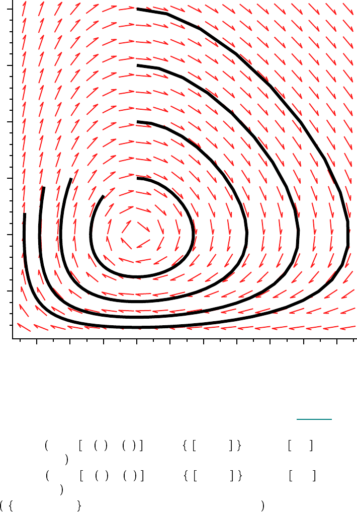
Only slight alterations are needed for higher-order equations, or for systems. To illustrate, consider
the predator-prey system
SYS d diff P t , t = p t $P t
K
P t , diff p t , t = 2$ p t
K
2$ P t
$p t ;
SYS :=
d
dt
P t = p t P t
K
P t ,
d
dt
p t = 2 p t
K
2 p t P t
where P denotes the size of the predator population, p is the size of the prey population and t is time.
A sampling of solution curves in phase-space can be created by specifying a set of initial conditions
using the sequence operator $ and the desired scene. (The subcommand 0, 1, k / 2 $ k = 2 ..6
below is a shortcut to generate the initial conditions
0, 1, 1 , 0, 1, 3 / 2 , 0, 1, 4 / 2 , 0, 1, 5 / 2 , 0, 1, 6 / 2 , 0, 1, 3 / 2 .) The stepsize=0.1 is
included because the default stepsize produces a rather rough graph.
DEplot SYS, P t , p t , 0 ..4, 0, 1, k / 2 $ k = 2 ..6 , scene = P, p , stepsize
= 0.1, title = `Predator-Prey: Phase Portrait`, linecolor = BLACK ;
Maple Manual for Fundamentals of Differential Equations, 8e, and Fundamentals of Differential Equations and Boundary Value Problems, 6e.
74
Copyright © 2012 Pearson Education, Inc.
O O
O O
O O
P
0.4 0.6 0.8 1.0 1.2 1.4 1.6 1.8 2.0 2.2
p
0.5
1
1.5
2
2.5
3
Predator-Prey: Phase Portrait
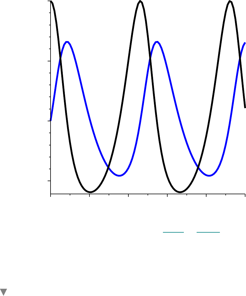
Plots of the individual solutions can be obtained by changing the scene. Here, individual plots of the
predator and prey are created, and then displayed in a single plot using the display command from
the plots package.
plotp d DEplot SYS, P t , p t , 0 ..10, 0, 1, 2 , scene = t, p , stepsize = 0.1,
linecolor = black :
plotP d DEplot SYS, P t , p t , 0 ..10, 0, 1, 2 , scene = t, P , stepsize = 0.1,
linecolor = blue :
display plotp, plotP , title = `Predator and Prey vs. Time` ;
Maple Manual for Fundamentals of Differential Equations, 8e, and Fundamentals of Differential Equations and Boundary Value Problems, 6e.
75
Copyright © 2012 Pearson Education, Inc.
O O
O O
O O
t
0 2 4 6 8 10
P
0.5
1
1.5
2
Predator and Prey vs. Time
This is only the beginning of what can be done with the DEplot and DEtools package. Please
consult the on-line help for additional information and a complete description of the available
options and examples.
?DEtools
?DEtools[DEplot]
Symbolic Solutions to Second Order ODEs and IVPs (Chapter 4 of
Nagle/Saff/Snider)
While Maple is quite happy to accept the inputs to its commands in almost any form, it is practically,
esthetically, and pedagogically preferable to use descriptive names for the individual parts of a
problem (e.g., the differential equation and boundary condition). To illustrate, let's find the general
solution to the non-homogeneous second order linear ODE x''C 4 x'C 4 x = 2 t$e
K
2 t
.
The differential equation can be entered as
Maple Manual for Fundamentals of Differential Equations, 8e, and Fundamentals of Differential Equations and Boundary Value Problems, 6e.
76
Copyright © 2012 Pearson Education, Inc.
O O
(2.2.5)(2.2.5)
(2.2.4)(2.2.4)
O O
(2.2.3)(2.2.3)
O O
O O
O O
(2.2.1)(2.2.1)
O O
(2.2.2)(2.2.2)
ODE d diff x t , t$2 C 4$diff x t , t C 4$x t = 2$t$exp
K
2$t ;
ODE :=
d
2
dt
2
x t C 4
d
dt
x t C 4 x t = 2 t e
K
2 t
and the general solution is found using dsolve.
GSOLN d dsolve ODE, x t ;
GSOLN := x t = e
K
2 t
_C2 C t e
K
2 t
_C1 C
1
3
t
3
e
K
2 t
Note that Maple introduces the symbols _C1 and _C2 as arbitrary constants. Any symbol
beginning with an underscore is effectively reserved for use only by Maple library code. It is not
available to users. Failure to observe this rule can lead to unexpected results.
The backslash key: \ , is the escape key to enter certain symbols in
2D input. For example, because the underscore is used to enter a
subscript, the entry _C1 is be made by typing \_C1.
The solution to an initial value problem can be obtained by including initial conditions in a set
containing the differential equation. For example, the initial conditions x 1 = 0, x' 1 = 1 can be
implemented as
IC d x 1 = 0, D x 1 = 1;
IC := x 1 = 0, D x 1 = 1
Note the use of D in the specification of the derivative condition (higher order derivative conditions
can be specified using @@, Maple's composition operator, e.g., (D@@2 x 0 = 3). Then, the
initial value problem is
IVP d ODE, IC ;
IVP :=
d
2
dt
2
x t C 4
d
dt
x t C 4 x t = 2 t e
K
2 t
, x 1 = 0, D x 1 = 1
and its solution is found using dsolve.
SOLN d dsolve IVP, x t ;
SOLN := x t =
1
3
e
K
2 t
K
3 C 2 e
K
2
e
K
2
K
t e
K
2 t
e
K
2
K
1
e
K
2
C
1
3
t
3
e
K
2 t
Expressions and Functions (Chapter 4 of Nagle/Saff/Snider)
Notice how the output from dsolve is a Maple equation (the reason for this choice will be apparent
when considering the solution to a system of differential equations). While there are specific cases
where these equations are useful, most circumstances call for either an expression or a function. The
key is to understand the structure of the output from dsolve.
Maple Manual for Fundamentals of Differential Equations, 8e, and Fundamentals of Differential Equations and Boundary Value Problems, 6e.
77
Copyright © 2012 Pearson Education, Inc.
(2.3.5)(2.3.5)
(2.3.4)(2.3.4)
O O
(2.3.3)(2.3.3)
O O
O O
O O
O O
(2.3.2)(2.3.2)
O O
(2.3.1)(2.3.1)
(2.3.6)(2.3.6)
Let's illustrate with the same example as above, with initial conditions specified, so that the
constants refer to the values of the solution and its first derivative at t = 1.
IC d x 1 = c
1
, D x 1 = c
2
;
IC := x 1 = c
1
, D x 1 = c
2
Note that these initial conditions are specified as a set, not an expression sequence. Thus, different
manipulations are required to express the final IVP as a set.
IVP d ODE union IC;
IVP :=
d
2
dt
2
x t C 4
d
dt
x t C 4 x t = 2 t e
K
2 t
, x 1 = c
1
, D x 1 = c
2
It is easiest to obtain the solution as an expression; it's just the right-hand side of the object that
Maple returns from dsolve.
X d rhs dsolve IVP, x t ;
X :=
1
3
e
K
2 t
K
3 c
2
K
3 c
1
C 2 e
K
2
e
K
2
K
t e
K
2 t
K
c
2
K
2 c
1
C e
K
2
e
K
2
C
1
3
t
3
e
K
2 t
When a Maple function is desired, it is most expedient to use unapply.
XX d unapply rhs dsolve IVP, x t , t ;
XX := t/
1
3
e
K
2 t
K
3 c
2
K
3 c
1
C 2 e
K
2
e
K
2
K
t e
K
2 t
K
c
2
K
2 c
1
C e
K
2
e
K
2
C
1
3
t
3
e
K
2 t
To illustrate a potential advantage of the use of unapply, consider a situation in which you wish to
include the constants as arguments to the solution function, e.g., x t; c
1
, c
2
, where c
1
and c
2
are
respectively, the values of the function and its first derivative at t = 1. Then you would use
XXX d unapply rhs dsolve IVP, x t , t, c
1
, c
2
;
XXX := t, c_1, c_2 /
1
3
e
K
2 t
K
3 c_2
K
3 c_1 C 2 e
K
2
e
K
2
K
t e
K
2 t
K
c_2
K
2 c_1 C e
K
2
e
K
2
C
1
3
t
3
e
K
2 t
and the resulting function, XXX, can be used to find the solution passing through the point 1, 0
with unit slope as follows
XXX t, 0, 1 ;
1
3
e
K
2 t
K
3 C 2 e
K
2
e
K
2
K
t e
K
2 t
e
K
2
K
1
e
K
2
C
1
3
t
3
e
K
2 t
The same computation using X and XX would appear as
Maple Manual for Fundamentals of Differential Equations, 8e, and Fundamentals of Differential Equations and Boundary Value Problems, 6e.
78
Copyright © 2012 Pearson Education, Inc.
O O
O O
O O
O O
(2.3.14)(2.3.14)
O O
O O
(2.3.10)(2.3.10)
O O
(2.3.13)(2.3.13)
(2.3.11)(2.3.11)
(2.3.12)(2.3.12)
O O
(2.3.8)(2.3.8)
(2.3.9)(2.3.9)
(2.3.7)(2.3.7)
subs c
1
= 0, c
2
= 1, X ;
1
3
e
K
2 t
K
3 C 2 e
K
2
e
K
2
K
t e
K
2 t
e
K
2
K
1
e
K
2
C
1
3
t
3
e
K
2 t
subs c
1
= 0, c
2
= 1, XX t ;
1
3
e
K
2 t
K
3 C 2 e
K
2
e
K
2
K
t e
K
2 t
e
K
2
K
1
e
K
2
C
1
3
t
3
e
K
2 t
Next, consider the problem of verifying that the solution is correct.
simplify subs x t = X, ODE ;
2 t e
K
2 t
= 2 t e
K
2 t
simplify subs x t = XX t , ODE ;
2 t e
K
2 t
= 2 t e
K
2 t
simplify subs x t = XXX t, c
1
, c
2
, ODE ;
2 t e
K
2 t
= 2 t e
K
2 t
To conclude this discussion, let's plot the solutions that have critical points (i.e., c
2
= 0) at (1,-1),
(1,1), and (1,3) using each of X, XX and XXX.
S1 d seq subs c
1
= C, c
2
= 0, X , C =
K
1, 1, 3 ;
S1 :=
1
3
e
K
2 t
K
9 C 2 e
K
2
e
K
2
K
t e
K
2 t
K
6 C e
K
2
e
K
2
C
1
3
t
3
e
K
2 t
,
1
3
e
K
2 t
K
3 C 2 e
K
2
e
K
2
K
t e
K
2 t
K
2 C e
K
2
e
K
2
C
1
3
t
3
e
K
2 t
,
1
3
e
K
2 t
3 C 2 e
K
2
e
K
2
K
t e
K
2 t
2 C e
K
2
e
K
2
C
1
3
t
3
e
K
2 t
S2 d seq subs c
1
= C, c
2
= 0, XX 't' , C =
K
1, 1, 3 ;
#The use of 't' is explained below.
S2 :=
1
3
e
K
2 t
K
9 C 2 e
K
2
e
K
2
K
t e
K
2 t
K
6 C e
K
2
e
K
2
C
1
3
t
3
e
K
2 t
,
1
3
e
K
2 t
K
3 C 2 e
K
2
e
K
2
K
t e
K
2 t
K
2 C e
K
2
e
K
2
C
1
3
t
3
e
K
2 t
,
1
3
e
K
2 t
3 C 2 e
K
2
e
K
2
K
t e
K
2 t
2 C e
K
2
e
K
2
C
1
3
t
3
e
K
2 t
S3 d seq XXX 't', C, 0 , C =
K
1, 1, 3 ;
S3 :=
1
3
e
K
2 t
K
9 C 2 e
K
2
e
K
2
K
t e
K
2 t
K
6 C e
K
2
e
K
2
C
1
3
t
3
e
K
2 t
,
Maple Manual for Fundamentals of Differential Equations, 8e, and Fundamentals of Differential Equations and Boundary Value Problems, 6e.
79

Copyright © 2012 Pearson Education, Inc.
O O
(2.3.15)(2.3.15)
O O
1
3
e
K
2 t
K
3 C 2 e
K
2
e
K
2
K
t e
K
2 t
K
2 C e
K
2
e
K
2
C
1
3
t
3
e
K
2 t
,
1
3
e
K
2 t
3 C 2 e
K
2
e
K
2
K
t e
K
2 t
2 C e
K
2
e
K
2
C
1
3
t
3
e
K
2 t
Note that the use of single quotes ( ' ) is needed so that the evaluation of t is delayed until after the
subs command is completed.
plot S3, t = 0 ..3, title = `Function: XXX(t,c1,c2)` ;
t
1 2 3
K
20
K
15
K
10
K
5
0
5
Function: XXX(t,c1,c2)
The structure of this solution (linear combination of a basis of solutions to the homogeneous
equation plus a particular solution) is evident in the solutions we have found. The individual
components can be easily extracted and manipulated. Here we demonstrate how a general solution is
used to determine the solution of a specific initial-value problem. Once the general solution is found,
GSOLN d rhs dsolve ODE, x t ;
GSOLN := e
K
2 t
_C2 C t e
K
2 t
_C1 C
1
3
t
3
e
K
2 t
Maple Manual for Fundamentals of Differential Equations, 8e, and Fundamentals of Differential Equations and Boundary Value Problems, 6e.
80
Copyright © 2012 Pearson Education, Inc.
O O
(2.3.23)(2.3.23)
(2.3.22)(2.3.22)
(2.3.25)(2.3.25)
O O
O O
O O
O O
O O
O O
O O
(2.3.20)(2.3.20)
(2.3.24)(2.3.24)
(2.3.19)(2.3.19)
O O
(2.3.21)(2.3.21)
O O
(2.3.18)(2.3.18)
O O
(2.3.16)(2.3.16)
(2.3.17)(2.3.17)
the two equations that must be satisfied by _C1 and _C2 can be constructed:
eq1 d subs t = 1, GSOLN = 3 ; eq2 d subs t = 1, diff GSOLN, t = 0 ;
eq1 := e
K
2
_C2 C e
K
2
_C1 C
1
3
e
K
2
= 3
eq2 :=
K
2 e
K
2
_C2
K
e
K
2
_C1 C
1
3
e
K
2
= 0
and solved
solC d solve eq1, eq2 , _C1, _C2 ;
solC := _C1 =
K
K
6 C e
K
2
e
K
2
, _C2 =
1
3
K
9 C 2 e
K
2
e
K
2
These solutions obviously simplify (but require an application of expand to force all simplifications)
.
solC d simplify expand solC ;
solC := _C1 = 6 e
2
K
1, _C2 =
K
3 e
2
C
2
3
Floating point approximations to these constants are obtained using evalf:
evalf solC ;
_C1 = 43.33433659, _C2 =
K
21.50050163
These values can be substituted back to GSOLN but the exact values are preferred. The solution to
the IVP is found to be
IVPsoln d factor subs solC, GSOLN ;
IVPsoln :=
1
3
e
K
2 t
K
9 e
2
C 2 C 18 t e
2
K
3 t C t
3
simplify IVPsoln
K
subs c
1
= 3, c
2
= 0, X ;
0
simplify IVPsoln
K
subs c
1
= 3, c
2
= 0, XX t ;
0
simplify IVPsoln
K
XXX t, 3, 0 ;
0
To conclude, let's see three different ways in which the terms contributing to the homogeneous and
particular solutions can be obtained. Working directly from the general solution we find
Xp d subs _C1 = 0, _C2 = 0, GSOLN ;
Xp :=
1
3
t
3
e
K
2 t
Xh d GSOLN
K
Xp;
Xh := e
K
2 t
_C2 C t e
K
2 t
_C1
X1 d subs _C1 = 1, _C2 = 0, Xh ;
Maple Manual for Fundamentals of Differential Equations, 8e, and Fundamentals of Differential Equations and Boundary Value Problems, 6e.
81
Copyright © 2012 Pearson Education, Inc.
O O
O O
O O
O O
(2.3.29)(2.3.29)
O O
O O
O O
(2.3.27)(2.3.27)
(2.3.31)(2.3.31)
(2.3.28)(2.3.28)
(2.3.26)(2.3.26)
(2.3.32)(2.3.32)
(2.3.30)(2.3.30)
O O
X1 := t e
K
2 t
X2 d subs _C1 = 0, _C2 = 1, Xh ;
X2 := e
K
2 t
Alternatively, the same information can be obtained directly from dsolve.
ODEh d lhs ODE = 0;
ODEh :=
d
2
dt
2
x t C 4
d
dt
x t C 4 x t = 0
IC1 d x 0 = 0, D x 0 = 1; X1 d rhs dsolve ODEh, IC1 , x t ;
IC1 := x 0 = 0, D x 0 = 1
X1 := t e
K
2 t
IC2 d x 0 = 1, D x 0 = 0; X2 d rhs dsolve ODEh, IC2 , x t ;
IC2 := x 0 = 1, D x 0 = 0
X2 := e
K
2 t
C 2 t e
K
2 t
ICp d x 0 = 0, D x 0 = 0; Xp d rhs dsolve ODE, ICp , x t ;
ICp := x 0 = 0, D x 0 = 0
Xp :=
1
3
t
3
e
K
2 t
Although, to be honest, in this case it is probably simplest to explicitly identify the appropriate terms
in the general solution and explicitly define the components of the solution.
x
1
d exp
K
2$t ; x
2
d t * exp
K
2$ t ; x
p
d
t
3
3
$exp
K
2$t ;
x
1
:= e
K
2 t
x
2
:= t e
K
2 t
x
p
:=
1
3
t
3
e
K
2 t
This example hopefully illustrates that while almost all manipulations can be done in Maple, some
steps should still be done by hand.
Additional information about dsolve is available from the on-line help (?dsolve). Note, in particular,
that dsolve may return an implicit solution or a solution in parametric form. Explicit solutions can,
sometimes, be coerced by using the optional argument explicit. Other optional arguments are
discussed later in this supplement.
?dsolve;
Maple Manual for Fundamentals of Differential Equations, 8e, and Fundamentals of Differential Equations and Boundary Value Problems, 6e.
82

Copyright © 2012 Pearson Education, Inc.
O O
O O
(2.4.1)(2.4.1)
O O
(2.4.4)(2.4.4)
O O
(2.4.5)(2.4.5)
(2.4.2)(2.4.2)
(2.4.3)(2.4.3)
(2.4.6)(2.4.6)
O O
O O
O O
O O
Systems of ODEs (Sections 5.2, 5.4 and 5.5 of Nagle/Saff/Snider)
Systems of ODEs are analyzed in a completely parallel manner. The system of equations is
specified as a set (with or without initial conditions); the dependent variables are also specified as a
set. To illustrate, consider the (linearized) model of a pendulum similar to Project D on page 238:
d
2
% t
dt
2
C 3$% t = 0 . This second-order equation is equivalent to the following system of first-
order equations:
restart;
SYS d diff theta t , t = v t , diff v t , t =
K
3$ theta t ;
SYS :=
d
dt
% t = v t ,
d
dt
v t =
K
3 % t
The dependent variables are:
FNS d theta t , v t ;
FNS := % t , v t
The general solution is found to be
SOL d dsolve SYS, FNS ;
SOL := % t = _C1 sin 3 t C _C2 cos 3 t , v t =
K
3
K
cos 3 t _C1
C _C2 sin 3 t
We are now in a position to understand why it is important that dsolve returns (a set of) equations.
Because a set is unordered, there is no reason to expect the elements of the solution set to appear in
the same order each time Maple is executed. That is, there is no "first'' term in the solution vector.
There is, nonetheless, a very simple means to ensure that the appropriate term from the solution is
extracted. It is still possible to obtain the individual component as either an expression
SOLV d subs SOL, v t ;
SOLV :=
K
3
K
cos 3 t _C1 C _C2 sin 3 t
or as a function
SOLT d unapply subs SOL, theta t , t ;
SOLT := t/_C1 sin 3 t C _C2 cos 3 t
Most systems of ODEs do not have explicit solutions. Maple has no difficulty producing series
solutions for systems, even nonlinear ones. We illustrate using the corresponding nonlinear
pendulum equation.
SYSnl d diff theta t , t = v t , diff v t , t =
K
3$ sin theta t ;
SYSnl :=
d
dt
% t = v t ,
d
dt
v t =
K
3 sin % t
Only a small number of terms will be needed to compare with the linearized solution.
Order d 3 :
Maple Manual for Fundamentals of Differential Equations, 8e, and Fundamentals of Differential Equations and Boundary Value Problems, 6e.
83
Copyright © 2012 Pearson Education, Inc.
O O
(2.4.7)(2.4.7)
(2.4.9)(2.4.9)
(2.5.2)(2.5.2)
O O
O O
(2.5.1)(2.5.1)
O O
O O
(2.4.8)(2.4.8)
O O
O O
SOLnl d dsolve SYSnl, FNS, type = series ;
SOLnl := % t = % 0 C v 0 t
K
3
2
sin % 0 t
2
C O t
3
, v t = v 0
K
3 sin % 0 t
K
3
2
cos % 0 v 0 t
2
C O t
3
SOLnlV d subs SOLnl, v t ;
SOLnlV := v 0
K
3 sin % 0 t
K
3
2
cos % 0 v 0 t
2
C O t
3
Comparisons with the solution to the linearized equation can be performed using the series
command, as follows
series SOLV, t = 0 ;
_C1 3
K
3 _C2 t
K
3
2
_C1 3 t
2
C O t
3
The real power of Maple for systems of ODEs is seen in its handling of numerical solutions. This
procedure will be demonstrated in the next section.
Numeric Solutions (Sections 3.6 and 5.3 of Nagle/Saff/Snider)
Numeric solutions to initial value problems can be used in a variety of ways in an introductory
course, including direction fields, qualitative behavior of solutions, existence theory, and regularity
theory. The dsolve command can be used for each of these topics. The default method used is rkf45,
a Maple implementation of the Fehlberg fourth-fifth order Runge-Kutta method.
Maple has built-in procedures for solving differential equations numerically. The dsolve command
with the options numeric and method=classical[choice] finds a numerical solution by using one of
the classical numerical methods. The choice foreuler implements the classical forward Euler method,
the choice heunform implements the improved Euler's method and the choice impoly implements the
modified Euler method. These methods will be demonstrated in a later section.
To begin our discussion, consider the initial-value problem
restart;
ODE d diff x t , t = x t
2
C t : IC d x 0 = 0 : IVP d ODE, IC ;
IVP :=
d
dt
x t = x t
2
C t, x 0 = 0
While this problem does have an explicit solution, it cannot be found using methods typically
learned in an introductory course. But, it is reasonable to ask if a solution does exist for all t O 0.
Numerical solutions can be used, with caution, to discuss questions of this type. The inclusion of
the optional argument type=numeric is the basic interface to the numerical version of dsolve.
numSOLN d dsolve IVP, x t , type = numeric ;
numSOLN := proc x_rkf45 ... end proc
Maple Manual for Fundamentals of Differential Equations, 8e, and Fundamentals of Differential Equations and Boundary Value Problems, 6e.
84
Copyright © 2012 Pearson Education, Inc.
(2.5.3)(2.5.3)
(2.5.4)(2.5.4)
O O
O O
O O
O O
The output from dsolve is now quite different. What this is saying is that numSOLN is a Maple
procedure that can be used to compute the solution at a given (numeric) value of t. For example:
numSOLN 0 ;
t = 0., x t = 0.
numSOLN 1 / 10 ;
t = 0.100000000000000, x t = 0.00500052836904142
Notice that the output from the procedure created by dsolve is a list of equations with one equation
for the independent variable and one equation for each dependent variable. The structure of this
solution is ideal for use with the subs command to extract specific components of a solution or even
to use the results in subsequent calculations.
The plot of a numerical solution can be created in a number of different ways. One of the simplest
ways is to use the odeplot command from the plots package, which must be loaded prior to use. The
basic syntax for odeplot expects the first argument to be the output from numeric dsolve. The
second argument should be a list of two or three expressions involving the dependent and
independent variables. For example:
with plots :
numSOLN d dsolve IVP, x t , type = numeric : odeplot numSOLN, t, x t , 0 ..1,
title = `Approx. solution to x' = x^2C1, x(0)=0` ;
Maple Manual for Fundamentals of Differential Equations, 8e, and Fundamentals of Differential Equations and Boundary Value Problems, 6e.
85
Copyright © 2012 Pearson Education, Inc.
O O
O O
O O
(2.5.5)(2.5.5)
t
0 0.2 0.4 0.6 0.8 1
x
0
0.1
0.2
0.3
0.4
0.5
Approx. solution to x' = x^2C1, x(0)=0
Both numeric dsolve and odeplot work equally well with higher-order equations and with systems.
The basic operations for a higher-order problem will be illustrated using the damped nonlinear
pendulum.
ODE d diff theta t , t$2 C 0.2 * diff theta t , t C sin theta t = 0 : IC
d theta 0 = Pi/ 4, D theta 0 = 0 : IVP d ODE, IC ;
IVP :=
d
2
dt
2
% t C 0.2
d
dt
% t C sin % t = 0, % 0 =
1
4
!, D % 0 = 0
PEND d dsolve IVP, theta t , type = numeric :
Multiple graphs are included in one plot when the second argument to odeplot is a list of lists. (Note
how the derivative of the solution is selected using diff .)
odeplot PEND, t, theta t , t, diff theta t , t , 0 ..10, title
= `Damped Nonlinear Pendulum` ;
Maple Manual for Fundamentals of Differential Equations, 8e, and Fundamentals of Differential Equations and Boundary Value Problems, 6e.
86
Copyright © 2012 Pearson Education, Inc.
O O
t
2 4 6 8 10
K
0.6
K
0.4
K
0.2
0
0.2
0.4
0.6
Damped Nonlinear Pendulum
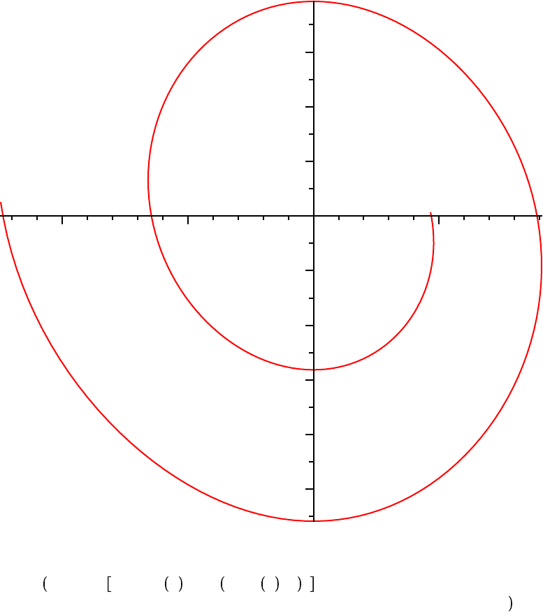
The phase portrait is also easy to create.
odeplot PEND, diff theta t , t , theta t ,
K
5 ..5, title
= `Damped Nonlinear Pendulum: phase plane` ;
Maple Manual for Fundamentals of Differential Equations, 8e, and Fundamentals of Differential Equations and Boundary Value Problems, 6e.
87
Copyright © 2012 Pearson Education, Inc.
O O
theta'
K
1
K
0.5
0
0.5
%
K
1
K
0.8
K
0.6
K
0.4
K
0.2
0.2
0.4
0.6
Damped Nonlinear Pendulum: phase plane
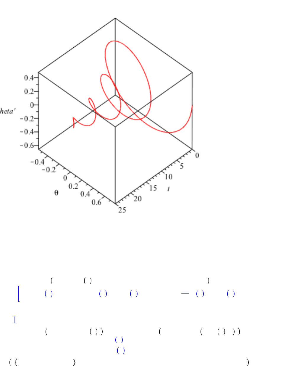
A three-dimensional view can sometimes be quite illustrative.
odeplot PEND, t, theta t , diff theta t , t , 0 ..25, title
= `Damped Nonlinear Pendulum: 3d view`, axes = BOXED, color = red ;
Maple Manual for Fundamentals of Differential Equations, 8e, and Fundamentals of Differential Equations and Boundary Value Problems, 6e.
88
Copyright © 2012 Pearson Education, Inc.
O O
O O
(2.5.7)(2.5.7)
O O
(2.5.6)(2.5.6)
Damped Nonlinear Pendulum: 3d view
You can now click on the image and rotate it by dragging the mouse.
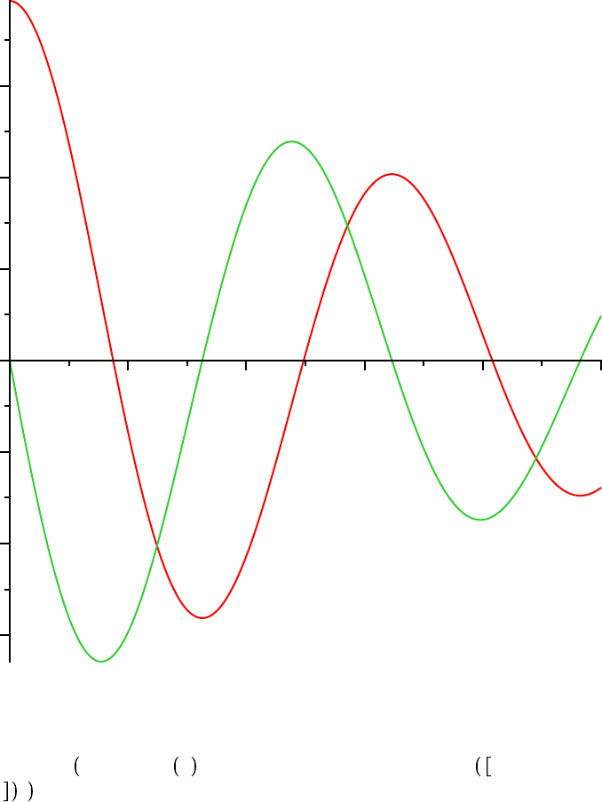
There are times when the standard output from numeric dsolve is not suitable for further processing.
The output = optional argument provides some flexibility. Specifying output = listprocedure will
cause dsolve to return a Maple list of procedures.
PEND2 d dsolve IVP, theta t , type = numeric , output = listprocedure ;
PEND2 := t = proc t ... end proc, % t = proc t ... end proc,
d
dt
% t = proc t
...
end proc
THETA d subs PEND2, theta t ; dTHETA d subs PEND2, diff theta t , t ;
THETA := proc t ... end proc
dTHETA := proc t ... end proc
plot THETA, dTHETA , 0 ..10, title = `Damped Nonlinear Pendulum: another view` ;
Maple Manual for Fundamentals of Differential Equations, 8e, and Fundamentals of Differential Equations and Boundary Value Problems, 6e.
89
Copyright © 2012 Pearson Education, Inc.
O O
(2.5.8)(2.5.8)
2 4 6 8 10
K
0.6
K
0.4
K
0.2
0
0.2
0.4
0.6
Damped Nonlinear Pendulum: another view
The output = argument is used when the value of the solution is needed only for specified values
of the independent variable. This method can be particularly useful when creating a table of data.
PEND3 d dsolve IVP, theta t , type = numeric, output = array i / 100. $ i = 320
..330 ;
Maple Manual for Fundamentals of Differential Equations, 8e, and Fundamentals of Differential Equations and Boundary Value Problems, 6e.
90
Copyright © 2012 Pearson Education, Inc.
O O
(2.5.11)(2.5.11)
O O
(2.5.12)(2.5.12)
(2.5.13)(2.5.13)
O O
(2.5.9)(2.5.9)
(2.5.10)(2.5.10)
O O
O O
(2.5.8)(2.5.8)PEND3 :=
t % t
d
dt
% t
3.20000000000000
K
0.562040594090033
K
0.0299450123596072
3.21000000000000
K
0.562313114439529
K
0.0245601766895983
3.22000000000000
K
0.562531829642660
K
0.0191840246328481
3.23000000000000
K
0.562696828567860
K
0.0138169935166268
3.24000000000000
K
0.562808204453003
K
0.00845951880330290
3.25000000000000
K
0.562866054905401
K
0.00311203409034493
3.26000000000000
K
0.562870481901806 0.00222502888967990
3.27000000000000
K
0.562821591788409 0.00755124026910515
3.28000000000000
K
0.562719495280840 0.0128661720451644
3.29000000000000
K
0.562564307464168 0.0181693980799930
3.30000000000000
K
0.562356147436138 0.0234604938145919
Extracting information from this table can be frustrating. Note that the structure of PEND3 is a two-
dimensional (column) array. The first element of PEND3 is the three-dimensional (row) vector
which describes the contents of the matrix contained in the second element of PEND3.
VARS d evalm PEND3 1, 1 ;
VARS :=
t % t
d
dt
% t
VARS 2 ;
% t
It is also possible to nest the indices to directly access entries in this data structure. For example, the
pendulum is at rest sometime between t = 3.25 and t = 3.26. At this time, the angle describing the
pendulum's position is approximately
rest d PEND3 2, 1 6, 2 C PEND3 2, 1 7, 2 / 2;
rest :=
K
0.562868268403604
which, converted to degrees, is
evalf rest $180 / Pi ;
K
32.2499761928740
To illustrate the use of numeric dsolve for a system, consider the second-order system
ODE d diff x t , t = 3$ x t
2
$y t
K
6$ y t
2
, diff y t , t =
K
x t
3
C 2
$ x t
2
C 2$ x t $y t
K
4$ y t : IC d x 0 = 1, y 0 = 0 : IVP d ODE,
IC ;
IVP :=
d
dt
x t = 3 x t
2
y t
K
6 y t
2
,
d
dt
y t =
K
x t
3
C 2 x t
2
Maple Manual for Fundamentals of Differential Equations, 8e, and Fundamentals of Differential Equations and Boundary Value Problems, 6e.
91
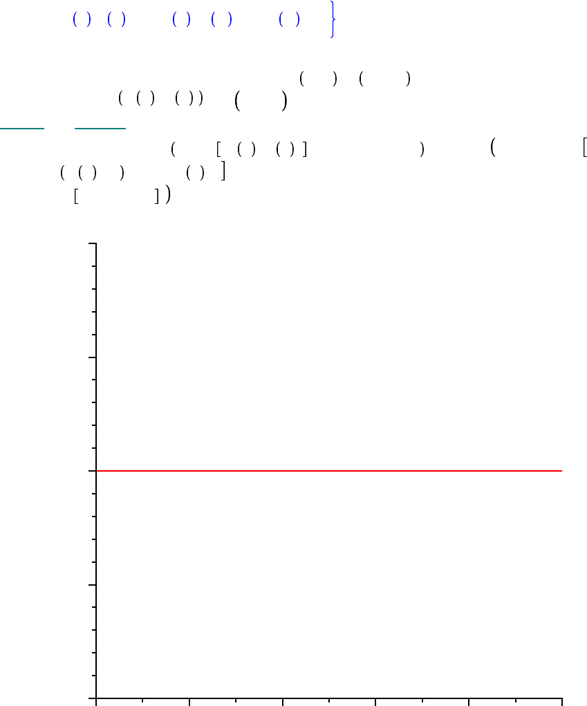
Copyright © 2012 Pearson Education, Inc.
O O
O O
O O
O O
O O
O O
C 2 x t y t
K
4 y t , x 0 = 1, y 0 = 0
The level curves of the (Liapunov) function L x, y = x
K
2
2
C 3 y
2
are trajectories for this
system. That is, L x t , y t = L x
0
, y
0
for all t O 0. This can be illustrated using numeric
dsolve and odeplot as follows.
numSOLN d dsolve IVP, x t , y t , type = numeric : odeplot numSOLN, t,
x t
K
2
2
C 3$ y t
2
, 0 ..10, title = `Values of L(x,y) = (x-2)^2 C 3y^2`, view
= 0 ..10, 0 ..2 ;
t
0 2 4 6 8 10
0
0.5
1
1.5
2
Values of L(x,y) = (x-2)^2 C 3y^2
?dsolve
?dsolve[numeric]
?dsolve[dverk78]
?plots[odeplot]
Maple Manual for Fundamentals of Differential Equations, 8e, and Fundamentals of Differential Equations and Boundary Value Problems, 6e.
92
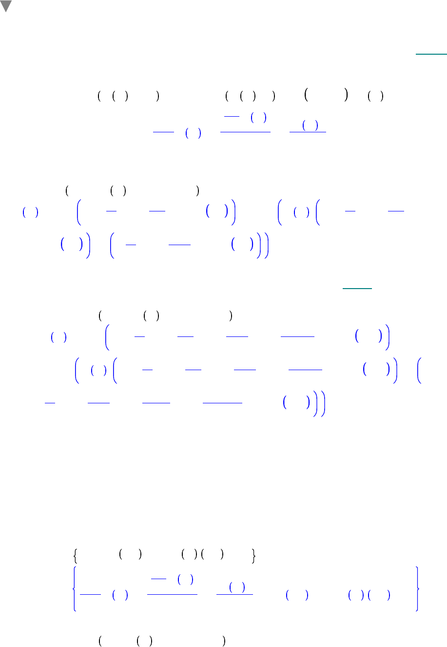
Copyright © 2012 Pearson Education, Inc.
O O
(2.6.4)(2.6.4)
O O
O O
O O
O O
(2.6.2)(2.6.2)
O O
O O
(2.6.5)(2.6.5)
(2.6.3)(2.6.3)
(2.6.1)(2.6.1)
Series Solutions (Chapter 8 of Nagle/Saff/Snider)
Some differential equations, and systems, are most approachable using power series techniques.
Maple provides access to this method by way of the type = series optional argument to dsolve.
Consider the differential equation, in normal form,
ODE d diff y x , x$2 C 1 / x $ diff y x , x
K
1 / x
2
C 1 $ y x = 0;
ODE :=
d
2
dx
2
y x C
d
dx
y x
x
K
y x
x
2
C 1
= 0
The first few terms of the power series, centered at x = 0, can be obtained with the command
dsolve ODE, y x , type = series ;
y x = _C1 1 C
1
4
x
2
K
3
64
x
4
C O x
6
C _C2 ln x 1 C
1
4
x
2
K
3
64
x
4
C O x
6
C
K
1
4
x
2
C
1
128
x
4
C O x
6
To obtain additional terms in the sequence, modify the system constant Order.
Order d 10 :
Y9 d dsolve ODE, y x , type = series ;
Y9 := y x = _C1 1 C
1
4
x
2
K
3
64
x
4
C
5
256
x
6
K
175
16384
x
8
C O x
10
C _C2 ln x 1 C
1
4
x
2
K
3
64
x
4
C
5
256
x
6
K
175
16384
x
8
C O x
10
C
K
1
4
x
2
C
1
128
x
4
C
1
1536
x
6
K
265
196608
x
8
C O x
10
Note that x = 0 is a regular singular point for this equation. Note also the structure of this solution.
The presence of the logarithmic factor is enlightening; that same term also complicates the
conversion of this solution from an equation whose RHS is of type series into an expression that
can be plotted, etc.
Series solutions centered at other points can be requested by specifying a full set of initial conditions
at the desired value of the independent variable. Here, the series expansion of the solution centered
at x =
K
1 will be produced.
IVP d ODE, y
K
1 = c
1
, D y
K
1 = c
2
;
IVP :=
d
2
dx
2
y x C
d
dx
y x
x
K
y x
x
2
C 1
= 0, y
K
1 = c
1
, D y
K
1 = c
2
Order d 6 :
Y5 d dsolve IVP, y x , type = series ;
Maple Manual for Fundamentals of Differential Equations, 8e, and Fundamentals of Differential Equations and Boundary Value Problems, 6e.
93
Copyright © 2012 Pearson Education, Inc.
(2.6.7)(2.6.7)
O O
O O
O O
(2.6.6)(2.6.6)
(2.6.5)(2.6.5)
O O
(2.6.8)(2.6.8)
Y5 := y x = c
1
C c
2
1 C x C
1
2
c
2
C
1
4
c
1
1 C x
2
C
5
12
c
2
C
1
6
c
1
1
C x
3
C
1
3
c
2
C
11
96
c
1
1 C x
4
C
127
480
c
2
C
1
12
c
1
1 C x
5
C O 1 C x
6
Here are two ways of obtaining the series solutions for two linearly independent solutions to this
ODE. First, it is possible to simply specify two different sets of values for the constants c
1
and c
2
.
Y5a d subs c
1
= 1, c
2
= 0, rhs Y5 ; Y5b d subs c
1
= 0, c
2
= 1, rhs Y5 ;
Y5a := 1 C
1
4
1 C x
2
C
1
6
1 C x
3
C
11
96
1 C x
4
C
1
12
1 C x
5
C O 1
C x
6
Y5b := 1 C x C
1
2
1 C x
2
C
5
12
1 C x
3
C
1
3
1 C x
4
C
127
480
1 C x
5
C O 1 C x
6
Alternatively, Maple can separately collect the terms involving c
1
and c
2
. But, before this collect can
be used, the solution must be converted to a polynomial. (As long as the O term is present, the
solution is an equation whose RHS is of type series.)
Y5 d convert rhs Y5 , polynom ;
Y5 := c
1
C c
2
1 C x C
1
2
c
2
C
1
4
c
1
1 C x
2
C
5
12
c
2
C
1
6
c
1
1 C x
3
C
1
3
c
2
C
11
96
c
1
1 C x
4
C
127
480
c
2
C
1
12
c
1
1 C x
5
Y5 d collect Y5, c
1
, c
2
;
Y5 :=
1
4
1 C x
2
C
1
6
1 C x
3
C
11
96
1 C x
4
C 1 C
1
12
1 C x
5
c
1
C
5
12
1 C x
3
C 1 C x C
1
2
1 C x
2
C
127
480
1 C x
5
C
1
3
1 C x
4
c
2
Note that the ordering of the terms in this last expression is less than optimal. (Controlling the order
of terms in a polynomial is not a simple task in Maple.)
plot map convert, Y5a, Y5b , polynom , x =
K
2 ..1, title
= `Linearly Independent Solution` ;
Maple Manual for Fundamentals of Differential Equations, 8e, and Fundamentals of Differential Equations and Boundary Value Problems, 6e.
94
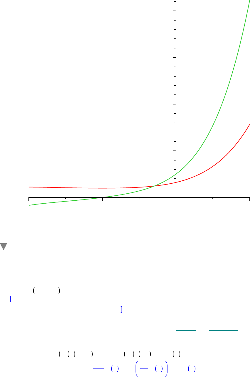
Copyright © 2012 Pearson Education, Inc.
(2.7.1)(2.7.1)
O O
(2.7.2)(2.7.2)
O O
O O
x
K
2
K
1
0
1
5
10
15
20
Linearly Independent Solution
Laplace Transforms (Chapter 7 of Nagle/Saff/Snider)
All uses of Laplace transforms should begin by reading the integral transform library into the Maple
session.
with inttrans ;
addtable, fourier, fouriercos, fouriersin, hankel, hilbert, invfourier, invhilbert, invlaplace,
invmellin, laplace, mellin, savetable
The two commands that form the Laplace transform pair are laplace and invlaplace. These
commands can be used explicitly or implicitly to solve a differential equation. To illustrate both
approaches, consider the problem of determining the general solution to
ODE d diff y t , t$2 C 3$ diff y t , t
K
4 $y t = 0;
ODE :=
d
2
dt
2
y t C 3
d
dt
y t
K
4 y t = 0
Maple Manual for Fundamentals of Differential Equations, 8e, and Fundamentals of Differential Equations and Boundary Value Problems, 6e.
95
Copyright © 2012 Pearson Education, Inc.
(2.7.3)(2.7.3)
(2.7.7)(2.7.7)
O O
O O
(2.7.4)(2.7.4)
O O
O O
(2.7.5)(2.7.5)
O O
O O
O O
O O
(2.7.6)(2.7.6)
One approach is to begin by applying the Laplace transform to this equation and solving for the
Laplace transform, Y s , of the solution y t .
lapODE d laplace ODE, t, s ;
lapODE := s
2
laplace y t , t, s
K
D y 0
K
s y 0 C 3 s laplace y t , t, s
K
3 y 0
K
4 laplace y t , t, s = 0
SOLY d solve lapODE, laplace y t , t, s ;
SOLY :=
3 y 0
C D y 0 C s y 0
s
2
C 3 s
K
4
Next, the inverse Laplace transform is applied to find the solution y t .
SOLy d invlaplace SOLY, s, t ;
SOLy :=
1
5
e
K
3
2
t
5 y 0 cosh
5
2
t C sinh
5
2
t 2 D y 0 C 3 y 0
or, as follows, in a form that is sometimes more useful.
collect SOLy, y 0 , D y 0 ;
1
5
e
K
3
2
t
5 cosh
5
2
t C 3 sinh
5
2
t y 0 C
2
5
e
K
3
2
t
sinh
5
2
t D y 0
Alternatively, a one-step solution is possible with the use of the method = laplace optional
argument to dsolve.
dsolve ODE, y t , method = laplace ;
y t =
1
5
e
K
3
2
t
5 y 0 cosh
5
2
t C sinh
5
2
t 2 D y 0 C 3 y 0
For additional assistance, consult the on-line help for dsolve
as well as the help pages for the individual commands
?inttrans[laplace];
?inttrans[invlaplace];
Maple Manual for Fundamentals of Differential Equations, 8e, and Fundamentals of Differential Equations and Boundary Value Problems, 6e.
96
