Copyright © 2012 Pearson Education, Inc.
1. Introduction
The study of mathematics can be greatly enhanced with the use of technology.
Differential equations, in particular, is a subject in which concepts can be more
thoroughly explored with the use of technology. The reason for the importance of
technology is that differential equations in many instances involve parameters that can be
varied. In addition, they usually involve symbolic and numerical calculations, many of
which may be intractable without the computer. Moreover they have solutions that should
be visualized graphically to understand behaviors.
Among the benefits of using technology in the teaching of differential equations are the
following. The student
• can see in easy fashion the behavior of solutions by means of graphs in the form of
direction fields and phase planes;
• will come to understand the role that parameters play in differential equations;
• will be able to examine “what-if” situations to discover properties of differential
equations;
• will be able to handle computationally intractable problems and generate numeric
solutions; and
• will be able to solve various applications of differential equations that involve
extensive computations.
This manual is written for the use of the computer algebra system Maple in differential
equations. The version of Maple used is Maple 14. Maple contains built-in libraries that
have many routines and commands useful in studying differential equations. Information
on the use and syntax of these commands and routines is available in a rather extensive
help directory.
When working with Maple, one is presented with a worksheet on which there can be
combined text, input, and output. (All of the labs in this manual were written on Maple
worksheets.) With ease, commands and text can be edited and corrected. It is easy to
copy and paste just as in a word processor. This makes it easy for students on the
worksheet to do the mathematics in Maple, display the results and the graphs, and then to
make comments and summaries of what they have learned.
There are two introductory chapters that detail how to use Maple. One is a general
introductory chapter “Introduction to Maple” and the other is a more specific introduction
“Demonstrations on Using Maple in Calculus and Differential Equations”. Both of these
can be used for reference when the labs are used from the manual. However, a
preliminary reading of them together with trial executions of the commands given is very
beneficial for what follows in the manual.
Following the introductory chapters are the laboratories, which comprise the heart of the
manual. These cover most of the essential topics in an introductory course in differential
equations. Some labs are longer than others; some require more work than others. Each
Maple Manual for Fundamentals of Differential Equations, 8e, and Fundamentals of Differential Equations and Boundary Value Problems, 6e.
1
Copyright © 2012 Pearson Education, Inc.
lab introduces the concepts and demonstrates how Maple is used in the context, but then
requires the students to become involved in exploratory exercises and questions. It may
be appropriate to only use part of a given lab rather than to do all the exercises. The
instructor should use discretion on how to best use the labs and modify them as needed
for a given situation.
The last part of the manual provides additional project ideas. The projects given represent
diverse kinds of applications including chemical engineering, mathematical epidemiolo-
gy, special functions, electrical circuits, and athletics. A brief overview of each project is
given at the beginning. Students are also encouraged in this chapter to devise their own
projects and a process for doing this is given.
In summary, the objective of this manual is to help students use technology in the form of
Maple to aid them in understanding and enjoying the study of differential equations.
Although some effort must be exerted to learn the basics of Maple and work is needed to
accomplish the labs, the rewards are well worth the effort. Technology can greatly aid in
the comprehension of mathematics.
Maple Manual for Fundamentals of Differential Equations, 8e, and Fundamentals of Differential Equations and Boundary Value Problems, 6e.
2
Copyright © 2012 Pearson Education, Inc.
1. 1.
O O
2. Introduction to Maple, Part 1
Worksheet Mode
What is Maple? Maple is a computer algebra system (CAS). What is a CAS? As the name suggests, it is
a computer software program that manipulates sophisticated algebraic symbols and expressions -- saving
you the time, the tedium, and the frustration of doing these by hand. But as we shall see, it is much more. It
can do some very advanced, difficult calculations, generate impressive graphs, and generate numerical and
symbolic solutions to problems that may be intractable by hand. If used properly, a CAS allows you the
user to concentrate more on the concepts of mathematics rather than spending time doing endless, time-
consuming computations. A CAS is a software package that works directly with an expression as a basic
data structure (compare this to most software packages that require numeric data and perform numeric
operations on the data). Maple is one of several CASs; other major examples are Mathematica, Derive,
and MathCad. In this introductory section, the rudiments of using Maple are given.
Prior to attempting any CAS Exercises, spend a few minutes reading through this introduction to become
familiar with some of the basic features, commands, and structure of Maple.
2.1 Worksheet Mode vs Document Mode
The default mode for working in Maple is called Worksheet Mode. Using this mode text is typed in
what are called Text Groups and executable commands and expressions to be simplified are typed in
what are referred to as Execution Groups. The commands in an Execution Group are typed at an input
prompt as shown below. They are executed by pressing the [enter] key.
This document was created using Maple 11 in its default Worksheet Mode.
Maple 11 can also be used in what is called Document Mode. In this mode there are no input prompts.
The user toggles between text and executable mathematics by pressing the [F5] key or by pressing
[control-T] for text and [control-R] for mathematics. See the Introduction to Maple, Part 2 for more
information about Document mode.
For Macintosh users,the [command] key (the key with the apple symbol)
is used instead of [control].
When a Maple worksheet is executed by repeatedly pressing the enter key, the cursor will jump to the
next prompt > within the next execution group. The empty execution group above is to prevent Maple
from jumping too far on the worksheet and passing by the narrative. There are basically three types of
text on a worksheet: (1) inert text, (2) active Maple input, and (3) Maple output.
inert text or inert in-line Maple input: The text you are reading now is an example of inert
commentary text which can be input within an execution group by selecting Text in the
Maple Manual for Fundamentals of Differential Equations, 8e, and Fundamentals of Differential Equations and Boundary Value Problems, 6e.
3

Copyright © 2012 Pearson Education, Inc.
O O
1. 1.
O O
2. 2.
O O
(2.3)(2.3)
(2.2)(2.2)
2. 2.
(2.1)(2.1)
3. 3.
O O
Insert Menu, by clicking the Text button in the Context Bar above or typing [control-T]. To
input non-executable mathematical notation within your text such as ! = 2 arcsin 1 or an
expression like x
2
dx, you must remove the command prompt > by placing the cursor just to the
right of it and then select 2-D Math in the Insert Menu, clicking the Math button in the Context
Bar, or typing [control-R]. Inert Maple input in standard mathematical notation can then be
inserted in-line by clicking the Math button in the Context Bar or by selecting Maple Input in the
Insert Menu. Both commands create a box where you can enter Maple code, such as
Pi = 2$arcsin 1 or int x^ 2, x , which corresponds to the mathematical notation you seek to
input. You can also remove the execution group altogether to insert inert text by clicking the
execution group with the mouse and then hitting the keyboard [delete] key.
active text or active in-line Maple input: Active input is a mathematical statement you want
Maple to evaluate and may be input within an execution group by selecting 2-D Math in the
Insert Menu. The input text is italics and Maple evaluates the command when you hit enter.
Maple output: Output, by default, is blue in color and in typeset notation. You can change the
display of output by selecting Options/Output Display.
2.2 1D Input vs 2D Input
In a Maple 11 worksheet, executable commands and mathematical expressions can be entered in one of
two ways:
Using 1D Input, also referred to as Maple Notation.
Using 2D Input, an input style that was introduced in Maple 10.
Math inputs in the traditional Maple Notation look like this.
3 + 1/3;
10
3
sin(Pi*x);
sin ! x
Note that 1D input prefers a terminating symbol, either a semicolon, or a colon (to suppress output).
1234567/89101112
Warning, inserted missing semicolon at end of statement
1234567
89101112
The same three commands have the following appearance when 2D input is the chosen style for math
entries. Note that no terminating punctuation is required. It is assumed that a semicolon is wanted, a
colon can be used to suppress output.
Maple Manual for Fundamentals of Differential Equations, 8e, and Fundamentals of Differential Equations and Boundary Value Problems, 6e.
4
Copyright © 2012 Pearson Education, Inc.
O O
O O
(3.1.1)(3.1.1)
(2.5)(2.5)
O O
O O
O O
(2.4)(2.4)
O O
(3.1.3)(3.1.3)
(2.6)(2.6)
O O
(3.1.2)(3.1.2)
3 C
1
3
10
3
sin ! x
sin ! x
1234567
89101112
1234567
89101112
The keyboard strokes for the first and third 2D inputs are the same as the the ones that were used for
the 1D inputs. In the second input, sin ! x , the ! symbol was entered by typing Pi, pressing the
escape key, [esc], to bring up a contextual menu, and then pressing [enter] to enter the first item on the
menu. Henceforth we refer shall refer to this sequence of steps as "press [esc]/[enter]".
Note also that a space was added between the ! and the x in the sin entry. This is to ensure that they are
multiplied.
2D input style is the default for a math entry in a Maple 11 Worksheet.
Consequently, this is the style that is used in this introduction. Occasional
examples are given to illustrate the traditional 1D style. Additional information
about 2D input will be given when a math entry contains more complicated
mathematical expressions.
2.3 Maple Arithmetic
At the simplest level, you can think of Maple as a powerful calculator that can do symbolic (exact)
manipulations as well as floating point (approximate) arithmetic.
Addition, Subtraction, Multiplication, and Division
The symbols + , - , * , and / are used for addition, subtraction, multiplication, and division
respectively. A space between two expressions is also used for multiplication in 2D input.
57575475849849885 C 74894985498544749598984
74895043074020599448869
87575750
K
48974759887309235722
K
48974759887221659972
99686861273254872299450000000000000
50000
1993737225465097445989000000000
Maple Manual for Fundamentals of Differential Equations, 8e, and Fundamentals of Differential Equations and Boundary Value Problems, 6e.
5

Copyright © 2012 Pearson Education, Inc.
(3.2.1)(3.2.1)
O O
O O
(3.2.2)(3.2.2)
O O
(3.2.4)(3.2.4)
O O
O O
O O
(3.2.5)(3.2.5)
(3.2.3)(3.2.3)
Note that pressing the division symbol, / , automatically puts in a fraction. Use the arrow keys to
move about and edit the terms in the fraction.
Powers
Use the caret symbol, ^ , to raise a number to a power. Two multiplication symbols can also be
used, **. In 2D math entry, an asterisk, * , prints as a centered dot.
444
4
38862602496
444$$4
38862602496
Exponentials, base e, can be handled with the exp function.
exp 2
e
2
As an alternative type e and press [esc]/[enter]. This enters the mathematical constant e. Then
exponentiate using ^ .
e
2
e
2
By typing exp then [esc]/[enter] there is no need to use the caret ^ to exponentiate.
e
3 C
2
3
e
11
3
Care must be taken in this regard. The math entries e
2
and e
2
evaluate entirely differently in Maple.
The former is simply the symbol e (the letter is in italics) raised to the power 2 while e
2
evaluates to
the square of the number e = 2.78182/ .
Palettes
Maple has several palettes that contain shortcuts to entering symbols and commands via the
keyboard. The palettes are docked in panels on the left and right sides of the worksheet window. If
the docks are not visible in your worksheet window click on the right-pointing triangle in the
bottom left corner of the window and/or on the left-pointing triangle in the bottom right corner.
Click on the other triangles to hide them from view.
The Expression palette can be used to enter powers, roots, elementary transcendental functions,
limits, derivatives, and other basic calculus-based expressions. For example, to enter the square root
390625 position the cursor at an input prompt and click on the symbol a in the palette. Type
390625 and then press the [enter] key to execute the entry. Your input and output should appear as
Maple Manual for Fundamentals of Differential Equations, 8e, and Fundamentals of Differential Equations and Boundary Value Problems, 6e.
6

Copyright © 2012 Pearson Education, Inc.
(3.4.2)(3.4.2)
O O
(3.4.3)(3.4.3)
(3.3.1)(3.3.1)
(3.4.4)(3.4.4)
(3.3.2)(3.3.2)
O O
O O
O O
O O
(3.4.1)(3.4.1)
O O
O O
390625
625
The square root template can also be entered directly from the keyboard by typing sqrt then pressing
[esc]-[enter].
When a palette generates a template that involves more than one argument, the [tab] key can be used
to move from one argument to the next. For example, to enter log
3
81 click on the log
b
a icon,
enter 3, press [tab], enter 81, then press [enter] to obtain
log
3
81
4
This can also be done directly from the keyboard by typing log_3, pressing the right arrow key,
then typing (81). Pressing the underscore key: _ , will move the input cursor to the subscript
position. Press the right arrow key to move it back to the baseline. Give it a try.
Maple palettes can be managed by choosing Palettes on the View menu.
Exact vs. Approximate Calculations
Maple is designed to provide exact answers to mathematical computations.
27
3 3
While the exact simplification in the previous example is useful, there are times when an exact
answer is not helpful. For example, the following rational number is returned unchanged because it
is already in reduced form.
5899
7
5899
7
There are several ways to instruct Maple to produce an approximate value for this number. Maple
will display a simplification as a floating point number if at least one number in the calculation is a
floating point number (i.e., contains a decimal point).
5899.
7
842.7142857
This does not always work as desired.
! C 3.
3
1
3
! C 1.000000000
Maple Manual for Fundamentals of Differential Equations, 8e, and Fundamentals of Differential Equations and Boundary Value Problems, 6e.
7

Copyright © 2012 Pearson Education, Inc.
(3.5.3)(3.5.3)
(3.4.7)(3.4.7)
(3.4.6)(3.4.6)
O O
O O
O O
O O
(3.5.2)(3.5.2)
O O
O O
O O
O O
(3.5.1)(3.5.1)
(3.4.5)(3.4.5)
(3.5.4)(3.5.4)
In a case like this the evalf command can be used to force Maple to evaluate using floating point
arithmetic.
evalf
! C 3
3
2.047197551
By default, Maple performs all floating point computations using 10 significant digits. Including a
second argument to the evalf command instructs Maple to use floating point numbers with the
specified number of significant digits.
evalf
! C 3
3
, 20
2.0471975511965977462
The entry evalf 20 / has the same effect. (See also the online help for Digits.)
evalf 20
! C 3
3
2.0471975511965977462
Using Previous Results, Labels
The percent symbol % represents the output of the last command executed by Maple.
625
125
5
At this point, the most recent result computed is 5. This can be squared with the entry
%
2
25
It is permissible to include more than one command in a single input region. Press [shift]-[enter] to
move the input cursor to the second line.
23.1 ;
2
K
9
4.806245936
K
7
Note that a semi-colon is used to separate the two commands. If a colon is used then the output to
the first command will be suppressed.
12
2
C 5
2
:
%
13
Maple Manual for Fundamentals of Differential Equations, 8e, and Fundamentals of Differential Equations and Boundary Value Problems, 6e.
8

Copyright © 2012 Pearson Education, Inc.
(3.5.5)(3.5.5)
O O
(3.5.6)(3.5.6)
O O
O O
(3.5.7)(3.5.7)
(4.2)(4.2)
O O
(4.1)(4.1)
O O
(4.3)(4.3)
O O
O O
O O
In this case the most recent result is 13. The next most recent result, which is the simplification of
12
2
C 5
2
, can be recalled with %%.
%% C 1
170
Every math output receives a label which can be entered in a subsequent input to refer to that output.
Labels are entered by choosing Label on the Insert menu or by pressing the keyboard equivalent,
Control-L (Command-L on a Macintosh).
(3.5.2)
5
It is not necessary to put multiple inputs on separate lines. They must, however, be separated by
either a semi-colon or a colon.
36; % ; % C %%
36
6
42
Note that when there are multiple outputs in an Execution Group, only the last output gets assigned
a label.
2.4 Assigning Names
The Maple command for assigning a value to a name is the two-character sequence " := ''. The single
character " = '' is used to form equations or to test for equality of two objects. Names generally consist
of a letter followed by one or more letters and numbers. Maple is case-sensitive -- the names x and X
are different, pi and Pi are not the same.
The commands to assign x the value 2 and y the value 3 are
x d 2; y d 3
x := 2
y := 3
The name prod will be assigned to the product of x and y
prod d x$y
prod := 6
From now on, the name prod will be replaced with this value. Thus,
prod
6
and, if the value of x is changed, the value of prod is not affected.
x d 9;
Maple Manual for Fundamentals of Differential Equations, 8e, and Fundamentals of Differential Equations and Boundary Value Problems, 6e.
9
Copyright © 2012 Pearson Education, Inc.
O O
O O
O O
(4.6)(4.6)
(4.5)(4.5)
(4.1.1)(4.1.1)
O O
(4.4)(4.4)
(4.8)(4.8)
O O
O O
O O
(4.7)(4.7)
O O
O O
prod
x := 9
6
The unassign command removes assignments that have been made. (To erase all assignments, it is
easier to use the restart command.)
unassign 'x', 'y', 'prod'
x, y, prod
x, y, prod
If prod is defined before assigning values to x and y,
prod d x$y
prod := x y
then when values are assigned to x and y, these values are used to compute the current value of prod.
x d 10;
y d 9;
prod
x := 10
y := 9
90
And, if one or both of x and y are changed, the value of prod changes as well.
x d 3;
prod
x := 3
27
The difference in these two examples is whether the names used in the definition of prod have values at
the time of definition.
A Reminder: Suppressing Output
If you wish to suppress the display of results of a command, use a colon to terminate the command.
x d 90 : y d 30 :
prod
2700
2.5 Maple Commands
restart
Maple Manual for Fundamentals of Differential Equations, 8e, and Fundamentals of Differential Equations and Boundary Value Problems, 6e.
10
Copyright © 2012 Pearson Education, Inc.
O O
O O
O O
O O
(5.1.3)(5.1.3)
(5.1.2)(5.1.2)
(5.1.5)(5.1.5)
(5.1.7)(5.1.7)
(5.1.1)(5.1.1)
O O
O O
O O
(5.1.6)(5.1.6)
(5.1.4)(5.1.4)
The above command clears Maple current memory.
Built-In Commands and Constants
Maple commands consist of a string of letters (and numbers) followed by one or more arguments
enclosed in round brackets (parentheses). The evalf and unassign commands have already been
encountered in this worksheet. Here are a few more examples.
If m and n are integers, m % n, the math entry $ m ..n returns the sequence of all integers from m
to n inclusive.
nums d$ 1 ..10
nums := 1, 2, 3, 4, 5, 6, 7, 8, 9, 10
The dollar sign is called the repetition operator. Here are two more examples.
morenums d k
2
K
8 k C 1 $ k =
K
6 ..6
morenums := 85, 66, 49, 34, 21, 10, 1,
K
6,
K
11,
K
14,
K
15,
K
14,
K
11
blue$6
blue, blue, blue, blue, blue, blue
If numseq represents a sequence of numbers, then min numseq will return the smallest number in
numseq.
min nums ;
min morenums
1
K
15
Warning: Errant Spaces in 2D Input
When entering a Maple command or function using 2D input be careful to
ensure that there are no spaces between the name of the command/function
and the left parenthesis that encloses its argument or arguments. A space in
2D math entry is interpreted as implied multiplication and an error will
result. See the next entry.
min nums
min 1, 2, 3, 4, 5, 6, 7, 8, 9, 10
Extra spaces in 1D input are generally ignored by the parser.
min (nums);
1
To find the smallest number in a set or a list, the surrounding brackets must be eliminated to obtain a
sequence of numbers.
L d 3, 5, 3, 7
L := 3, 5, 3, 7
Maple Manual for Fundamentals of Differential Equations, 8e, and Fundamentals of Differential Equations and Boundary Value Problems, 6e.
11
Copyright © 2012 Pearson Education, Inc.
O O
(5.1.8)(5.1.8)
(5.1.9)(5.1.9)
O O
O O
O O
O O
O O
(5.1.11)(5.1.11)
(5.1.10)(5.1.10)
(5.1.12)(5.1.12)
min L
3
The op procedure can be applied to L to access its "operands". Then min will do its job.
op L ;
min op L
3, 5, 3, 7
3
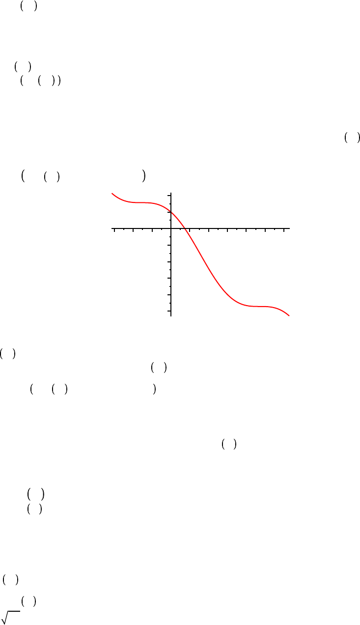
The next entry shows how to use the plot command to plot the expression cos x
K
x for values of
x from
K
! to 2 !.
plot cos x
K
x, x =
K
! ..2 !
x
K
3
K
2 1 2 3 4 5 6
K
5
K
4
K
3
K
2
K
1
1
2
We want to find the x value where the graph crosses the horizontal axis. In Maple the equation
cos x
K
x = 0 is represented exactly as it would be written by hand. The following fsolve
command locates the solution to cos x = x = 0 between x = 0 and x = 2.
fsolve cos x
K
x = 0, x = 0 ..2
0.7390851332
As mentioned previously, some Maple names are predefined to standard constants. For example, Pi
is ! and the natural base e can be obtained with exp 1 . These can also be entered in 2D input using
the expression palette or from the keyboard using Pi [esc]/[enter] and e [esc]/[enter] respectively.
This is what we did below.
evalf ! ;
evalf e
3.141592654
2.718281828
The square foot function is entered as sqrt, so the square root of a number can be obtained by typing
sqrt x . In 2D entry type sqrt [esc]/[enter] to obtain the square root template.
sqrt 4 ;
4
2
2
Maple Manual for Fundamentals of Differential Equations, 8e, and Fundamentals of Differential Equations and Boundary Value Problems, 6e.
12

Copyright © 2012 Pearson Education, Inc.
O O
O O
(5.1.15)(5.1.15)
O O
(5.1.16)(5.1.16)
(5.1.13)(5.1.13)
(5.1.14)(5.1.14)
O O
O O
O O
O O
Maple has no trouble handling the square root of a negative number. In output the imaginary unit is
denoted I.
K
1
I
This can also be used in an input.
1
K
I
1 C I
K
I
Alternatively, one can enter the imaginary unit by typing i [esc]/[enter] to obtain the symbol i. (2D
input only.)
1
K
i
1 C i
K
I
One more example.
K
4
2 I
Command Options
Many Maple commands, particularly the plotting commands, accept optional arguments for
customizing the output. For example, the option linestyle = 3 plots the expression using a dashed
line. The equation linestyle = dash can also be used.
plot sin x C cos 2 x , x = 0 ..2 !, linestyle = 3
x
1 2 3 4 5 6
K
2
K
1
0
1
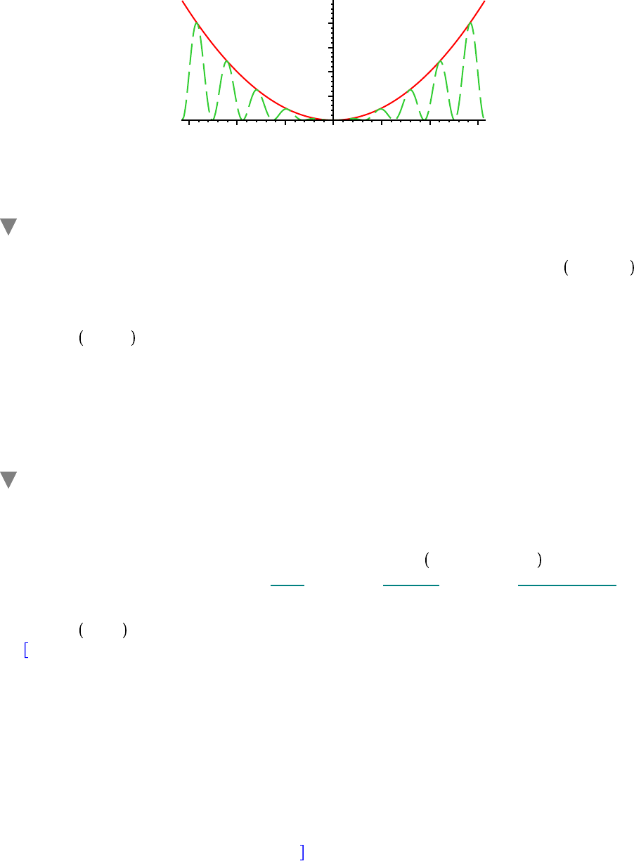
In the next plot command, the two expressions x
2
and x
2
sin x
2
are plotted simultaneously with
the first curve appearing as a dashed line and the second as a solid line. (Although it is not apparent
in the printout of this worksheet, Maple displays the first plot in red and the second in green. An
optional equation of the form, say, color = black, blue , could be used to control the colors used in
the plot.
Note that the sequence of expressions to be plotted are placed inside of square brackets to form
what is referred to as a list.
plot x
2
, x
2
sin x
2
, x =
K
5 ! ..5 !, linestyle = 1, 3
Maple Manual for Fundamentals of Differential Equations, 8e, and Fundamentals of Differential Equations and Boundary Value Problems, 6e.
13
Copyright © 2012 Pearson Education, Inc.
O O
O O
O O
O O
(5.4.1)(5.4.1)
O O
x
K
15
K
10
K
5 0 5 10 15
50
100
150
200
Online Help
The Maple command for accessing information in the online help database is help keyword , or the
abbreviated form ?keyword. The help information appears in a separate browser window within
Maple. To return to an active worksheet, either close the help window or click on the worksheet.
help fsolve
?plot, color
The Help menu can also be used to access the online resources available to help a new, or veteran,
Maple user. This is particularly useful when a particular command name is not known.
Packages
In addition to the standard Maple functions available at the beginning of every Maple session, there
are an ever-growing number of additional functions and commands contained in packages that must
be loaded into the Maple session prior to their use. The with package_name command is used to
load a package. Libraries include the plots library, the DEtools library, the LinearAlgebra library, to
name a few. Here is the plots package.
with plots
animate, animate3d, animatecurve, arrow, changecoords, complexplot, complexplot3d,
conformal, conformal3d, contourplot, contourplot3d, coordplot, coordplot3d,
densityplot, display, dualaxisplot, fieldplot, fieldplot3d, gradplot, gradplot3d,
implicitplot, implicitplot3d, inequal, interactive, interactiveparams, intersectplot,
listcontplot, listcontplot3d, listdensityplot, listplot, listplot3d, loglogplot, logplot,
matrixplot, multiple, odeplot, pareto, plotcompare, pointplot, pointplot3d, polarplot,
polygonplot, polygonplot3d, polyhedra_supported, polyhedraplot, rootlocus,
semilogplot, setcolors, setoptions, setoptions3d, spacecurve, sparsematrixplot,
surfdata, textplot, textplot3d, tubeplot
The output of a successful with command is the list of commands that have been added to Maple's
memory. If this list is unwanted, use a colon to terminate the command.
One of the commands that is now defined is named implicitplot.
Maple Manual for Fundamentals of Differential Equations, 8e, and Fundamentals of Differential Equations and Boundary Value Problems, 6e.
14
Copyright © 2012 Pearson Education, Inc.
• •
• •
• •
O O
(5.5.2)(5.5.2)
O O
O O
• •
O O
(5.5.3)(5.5.3)
O O
• •
(5.5.1)(5.5.1)
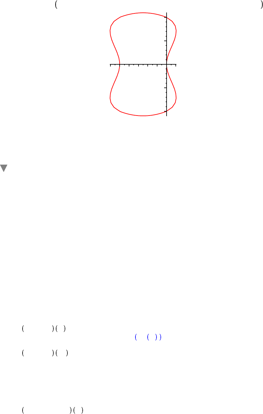
implicitplot x
2
C y
4
= y
2
K
x, x =
K
1.3 ..0.3, y =
K
1.2 ..1.2, scaling = constrained
x
K
1.0
K
0.4
0
0.2
y
K
1
K
0.5
0.5
1
The scaling = constrained option instructs Maple to use the same scaling for each axis in the plot.
Creating Functions
Built into Maple are the basic functions, relational operators, and logical operators. They are denoted
as follows.
trigonometric: sin, arcsin, cos, arccos, tan, arctan, csc, arccsc, sec, arcsec, cot, arccot
relational: <, <=, >, >=, = , <> (not equal)
logical: and, or, not
transcendental: ln, log[b], exp
hyperbolic: sinh, cosh, tanh, sech, coth, csch
There are many other functions as well.
Functions can be composed using the composition operator @. For examples
cos@sin x ;
cos sin x
cos@sin Pi ;
1
Repeated compositions can be performed by @@2, @@@3, ... or multiple use of the @ operator as
shown,
cos@sin@cos x ;
Maple Manual for Fundamentals of Differential Equations, 8e, and Fundamentals of Differential Equations and Boundary Value Problems, 6e.
15
Copyright © 2012 Pearson Education, Inc.
(5.5.10)(5.5.10)
(5.5.5)(5.5.5)
O O
(5.5.7)(5.5.7)
(5.5.4)(5.5.4)
O O
O O
(5.5.11)(5.5.11)
O O
O O
O O
O O
O O
(5.5.6)(5.5.6)
(5.5.3)(5.5.3)
(5.5.12)(5.5.12)
O O
(5.5.9)(5.5.9)
(5.5.8)(5.5.8)
cos sin cos x
exp tan @sin x ;
e
tan sin x
cos@@2 x ;
cos
2
x
cos@cos x ;
cos
2
x
You can create your own Maple commands, including implementations of mathematical functions.
For example, the function f x = x
2
sin x
2
can be defined using the assignment operator, d , as
shown in the next math entry.
f x d x
2
sin x
2
f := x/x
2
sin x
2
A dialogue will appear asking for confirmation that a function definition is the desired action as
opposed to simply assigning the name f x to the expression x
2
sin x
2
. The output confirms that
f is the name of a transformation that takes an input x and returns x
2
sin x
2
.
It is also possible to define the same function f using the arrow notation in the input. Press the
minus sign and the right arrow bracket: - > , to make the right arrow in the input.
f d x/x
2
sin x
2
f := x/x
2
sin x
2
If 1D math entry is used, then the function f is defined like this.
f := x -> x^2*sin(x)^2;
f := x/x
2
sin x
2
The variable x in the definition of f is a dummy variable; it is replaced by whatever object appears
as the first argument in f .
f y
y
2
sin y
2
f fred
fred
2
sin fred
2
f
!
2
1
4
!
2
Notice how Maple automatically simplifies the value of the function when possible.
Maple Manual for Fundamentals of Differential Equations, 8e, and Fundamentals of Differential Equations and Boundary Value Problems, 6e.
16
Copyright © 2012 Pearson Education, Inc.
(5.5.16)(5.5.16)
(5.5.14)(5.5.14)
O O
O O
O O
(5.5.15)(5.5.15)
O O
O O
(5.5.18)(5.5.18)
O O
O O
O O
(5.5.17)(5.5.17)
(5.5.13)(5.5.13)
To plot the graph of the function you can use either of the following commands.
plot f x , x =
K
5 ! ..5 !
x
K
15
K
10
K
5 0 5 10 15
50
100
150
200
plot f,
K
5 ! ..5 !
K
15
K
10
K
5 0 5 10 15
50
100
150
200
The plots are identical, except for the label on the horizontal axis.
Also, with functions, we can easily consider more variables as shown here,
g d x, y / x$sqrt y ;
g := x, y /x y
h d x, y, z / abs ln x $cos y $exp z ;
h := x, y, z / ln x cos y e
z
We then invoke a function by name and respective input variables,
g 5, 17 ;
5 17
g 5.0, 17 ;
5.0 17
g 5, 17.0 ;
20.61552813
evalf g 5, 17 ;
20.61552813
Maple Manual for Fundamentals of Differential Equations, 8e, and Fundamentals of Differential Equations and Boundary Value Problems, 6e.
17
Copyright © 2012 Pearson Education, Inc.
O O
(5.5.21)(5.5.21)
O O
(5.5.23)(5.5.23)
(5.5.19)(5.5.19)
(5.5.20)(5.5.20)
O O
O O
O O
(5.5.22)(5.5.22)
O O
where the data type of the input determines the form of the computed result. For example, the
function g 5, 17 has two integer inputs, 5 and 17, and because of this, performed exact
computations. Evaluation of g 5.0, 17 and g 5, 17.0 demonstrates that floating-point data types
5.0 and 17.0 sometimes activate Maple to perform exact computations and sometimes activate
Maple to perform approximate calculations while evalf (evaluate as floating-point) always results in
approximate calculations.
The unapply command provides a second way to define a function in Maple. It converts an
assignment into a function. For example if h is assigned to the expression x
3
C 2, then we can
convert it into a function of x as follows.
h d x
3
C 2;
h := x
3
C 2
h d unapply h, x ; #This makes h into a function of x.
h := x/x
3
C 2
h 4 ;
66
The absolute value symbol in the following definition is entered by typing the vertical line symbol: |
.
g d unapply x
2
K
4 , x
g := x/ x
2
K
4
The absolute value function can also be entered in Maple as abs x .
h d unapply x abs sin x , x
h := x/x sin x
plot h,
K
3 ! ..3 !
K
8
K
6
K
4 2 4 6 8
K
6
K
4
K
2
2
4
6
The unapply definition is often used when it is necessary make a function out of some expression
that appears as part of a previous output, or requires some simplification. Here is an example. The
solve command is used to solve an equation and one of the solution expressions is made into a
function named F using unapply.
Maple Manual for Fundamentals of Differential Equations, 8e, and Fundamentals of Differential Equations and Boundary Value Problems, 6e.
18
Copyright © 2012 Pearson Education, Inc.
O O
(5.5.25)(5.5.25)
O O
(6.1.3)(6.1.3)
O O
O O
O O
O O
O O
(5.5.24)(5.5.24)
(6.1.1)(6.1.1)
(6.1.2)(6.1.2)
soln d solve x
2
C x
K
4 y = 0, x
soln :=
K
1
2
C
1
2
1 C 16 y ,
K
1
2
K
1
2
1 C 16 y
F d unapply soln 1 , y
F := y/
K
1
2
C
1
2
1 C 16 y
Important Observation. When a sequence has a name, like soln above, then the j
th
expression in the
sequence can be accessed using the entry soln j . More about this below.
2.6 Lists and Sets
Definitions
In addition to expression sequences, two of the most important data structures in Maple are the list
and the set. A list is an expression sequence contained in square brackets, exprseq , and a set is
an unordered sequence contained in braces exprseq . (An expression sequence is a comma-
separated collection of numbers, names, equations, or other Maple objects.)
The next math entry defines a set named S and a list named L.
S d 1, 3, 111 ;
L d $ 6 ..10
S := 1, 3, 111
L := 6, 7, 8, 9, 10
Notice that the elements of a list or a set can be any valid Maple object, including another list or set.
SS d S, L
SS := 6, 7, 8, 9, 10 , 1, 3, 111
LL d S, L
LL := 1, 3, 111 , 6, 7, 8, 9, 10
Look carefully at the previous results. Even though the only difference in the definition of LL and
SS is the type of brackets, the order of the elements in SS might appear in the opposite of the order
in which they appeared in the definition. Recalling that the elements of a set are not ordered, this is
not surprising. (It should also not be surprising to know that the order in which Maple displays the
elements of a set can change from one session to another.)
Creating Lists and Sets
Except for the surrounding brackets, lists and sets are created in exactly the same ways. We have
already seen how to create lists and sets from explicit collections of numbers and with the repetition
operator, $ . The seq and map command provide two additional methods for creating lists and sets.
The seq command generates an expression sequence consisting of terms formed from the first
Maple Manual for Fundamentals of Differential Equations, 8e, and Fundamentals of Differential Equations and Boundary Value Problems, 6e.
19

Copyright © 2012 Pearson Education, Inc.
(6.3.6)(6.3.6)
(6.3.1)(6.3.1)
O O
O O
O O
O O
O O
(6.3.2)(6.3.2)
(6.3.7)(6.3.7)
O O
(6.3.5)(6.3.5)
(6.3.4)(6.3.4)
O O
(6.3.3)(6.3.3)
O O
O O
O O
The same plot could also have been created directly with either of the following variations of the
plot command. The output of these commands is suppressed by terminating the commands with a
colon. The first shows how to plot a polar function by specifying only the radius function and the
range for the polar angle.
plot r t , t = 0 ..2 !, coords = polar :
The second shows how the function can be displayed as a parametric curve.
plot r t $cos t , r t $sin t , t = 0 ..2 ! :
Extracting Elements of a List or Set
Much more than plotting can be done with a list or set. For example, the third element of the list
named pts can be accessed as
pts 3
9
Notice that it does not make sense to talk about the third element of a set. While Maple will not
object to this, you should not expect to receive the same result every time the command is executed.
The select and remove commands are designed to extract elements of a set that meet certain criteria.
For example, the subset of S (defined above) that contains all elements that are in the open interval
K
10, 10 can be found as follows.
S
1, 3, 111
select x/ x ! 10, S
1, 3
The number of elements in a list or set can be determined with the nops command.
nops rose4
101
Recall that each element of rose4 is an ordered pair—actually, a two-element list.
rose4 10
sin
9
25
! cos
9
50
! , sin
9
25
! sin
9
50
!
A floating-point approximation to this point is
evalf %
0.7639707480, 0.4848305795
The y-coordinate of the tenth element of the list is
rose4 10, 2
Maple Manual for Fundamentals of Differential Equations, 8e, and Fundamentals of Differential Equations and Boundary Value Problems, 6e.
21
Copyright © 2012 Pearson Education, Inc.
O O
O O
(6.3.13)(6.3.13)
O O
(6.3.10)(6.3.10)
(6.3.14)(6.3.14)
O O
(6.3.12)(6.3.12)
(6.3.8)(6.3.8)
O O
O O
O O
(6.3.7)(6.3.7)
O O
O O
(6.3.9)(6.3.9)
(6.3.15)(6.3.15)
(6.3.11)(6.3.11)
sin
9
25
! sin
9
50
!
Negative indices can be used to reference elements relative to the end of the list. For example, the
last point in rose4 is
rose4
K
1
0, 0
This can also be obtained using
rose4 nops rose4
0, 0
The first ten elements of rose4 can be specified using rose4 1 ..10 . The floating point
approximations to the x-coordinates of each of these points can be obtained with
evalf seq rose4 i, 1 , i = 1 ..10
0., 0.1250859171, 0.2467288932, 0.3616040548, 0.4666184965, 0.5590169945,
0.6364758026, 0.6971812263, 0.7398902011, 0.7639707480
The dollar sign operator fails here.
evalf rose4 i, 1 $ i = 1 ..10
Error, invalid subscript selector
This is because $ attempts to evaluate rose4 i, 1 before i = 1 has been substituted into the
expression. This is referred to as "premature evaluation". Premature evaluation can be avoided by
enclosing rose4 i, 1 in single quotes thereby delaying evaluation until the substitution has been
made. See the next input.
evalf 'rose4 i, 1 ' $ i = 1 ..10
0., 0.1250859171, 0.2467288932, 0.3616040548, 0.4666184965, 0.5590169945,
0.6364758026, 0.6971812263, 0.7398902011, 0.7639707480
Sets can also be manipulated using the standard set operators: union, intersect, and minus. Each
of these commands can be used both as an infix operator, following standard mathematical notation,
or as a prefix operator, which looks more program-like.
S union SS
1, 3, 111, 6, 7, 8, 9, 10 , 1, 3, 111
union S, SS
1, 3, 111, 6, 7, 8, 9, 10 , 1, 3, 111
S minus 1, 3
111
S intersect $ 2 ..10
3
With 1D input, the prefix use of an operator must be entered as follows, with backward quotes on
Maple Manual for Fundamentals of Differential Equations, 8e, and Fundamentals of Differential Equations and Boundary Value Problems, 6e.
22
Copyright © 2012 Pearson Education, Inc.
O O
O O
(6.4.2)(6.4.2)
(6.3.18)(6.3.18)
(6.3.20)(6.3.20)
(6.4.1)(6.4.1)
O O
(6.3.17)(6.3.17)
O O
(6.4.3)(6.4.3)
O O
O O
O O
O O
(6.3.19)(6.3.19)
O O
O O
(6.3.16)(6.3.16)
the command.
`union`(S,SS);
1, 3, 111, 6, 7, 8, 9, 10 , 1, 3, 111
Observe that the prefix forms of union and intersect can accept any number of sets.
SetSequence d seq $0 ..k , k = 2 ..4 ;
union SetSequence ;
intersect SetSequence
SetSequence := 0, 1, 2 , 0, 1, 2, 3 , 0, 1, 2, 3, 4
0, 1, 2, 3, 4
0, 1, 2
The map operator can be used to apply a command to every element of a list. The following
demonstrates this feature,
map sqrt, L ;
6 , 7 , 2 2 , 3, 10
evalf % ;
2.449489743, 2.645751311, 2.828427124, 3., 3.162277660
f d x/x
2
:
map f, (6.3.18) ;
6, 7, 8, 9, 10
Extracting Solutions to an Equation
When Maple finds the solution to an equation or system of equations, the default output is to
display the solutions as an expression sequence. This can be changed to a list or a set by inserting
the appropriate brackets around the solve (or fsolve) command.
In any event, if the solutions are named sol, then the j
th
term in the output can be obtained using the
entry sol j .
sol d fsolve x
2
= 3, x
sol :=
K
1.732050808, 1.732050808
sol 1
K
1.732050808
If the unknown or unknowns in the input are enclosed in set brackets, then the solutions will be
expressed in equation form, also enclosed in set brackets.
soln d fsolve x
2
C y = 3, x
K
y = 2 , x, y
soln := x = 1.791287847, y =
K
0.2087121525
Maple Manual for Fundamentals of Differential Equations, 8e, and Fundamentals of Differential Equations and Boundary Value Problems, 6e.
23
Copyright © 2012 Pearson Education, Inc.
(6.4.8)(6.4.8)
O O
(6.4.9)(6.4.9)
O O
O O
(6.4.4)(6.4.4)
O O
(6.4.5)(6.4.5)
O O
(6.4.10)(6.4.10)
(6.4.7)(6.4.7)
(6.4.6)(6.4.6)
O O
O O
The fsolve procedure usually returns just one approximate solution. The solve procedure always
attempts to return all of the exact solution values. The next entry applies solve to a system of two
equations in two unknowns. In this case the equations and the unknowns should be entered as sets.
ExactSoln d solve x
2
C y = 3, x
K
y = 2 , x, y
ExactSoln := x = RootOf _Z
2
C 5 _Z C 1 C 2, y = RootOf _Z
2
C 5 _Z C 1
For the sake of compactness, the exact solutions are presented in terms of the roots of the
polynomial z
2
C 5 z C 1. An application of the allvalues procedure asks Maple to display all of the
solutions that can be generated from the roots.
allvalues ExactSoln
x =
K
1
2
C
1
2
21 , y =
K
5
2
C
1
2
21 , x =
K
1
2
K
1
2
21 , y =
K
5
2
K
1
2
21
To extract the x value of the second solution one can use the substitute procedure, subs, as follows.
Note that the label of the last output has been used in lieu of the percent sign %.
subs (6.4.5) 2 , x
K
1
2
K
1
2
21
When fsolve is applied to a polynomial to find its roots, it will output approximations to all of the
real roots.
fsolve x
3
K
2 x C 2, x
K
1.769292354
Add the keyword complex and approximations to all of the roots will be displayed. The next entry
does this and, because the input is in set brackets, so is the output.
solns d fsolve x
3
K
2 x C 2, x, complex
solns :=
K
1.76929235423863, 0.884646177119316
K
0.589742805022205 I,
0.884646177119316 C 0.589742805022205 I
The solutions can be checked by using the map function to map the function x/x
3
K
2 x C 2 into
the set of solutions.
map x/x
3
K
2 x C 2, solns
0., 2.22044604925031 10
-16
C 0. I
We interpret both numbers in the last output set as 10 digit approximations to 0.
The next entry generates approximations to the four roots of the quartic polynomial x
4
K
3 x
2
C x.
The output is sequence named polysol.
polysol d fsolve x
4
K
3 x
2
C x, x
polysol :=
K
1.879385242, 0., 0.3472963553, 1.532088886
The largest element of this set can be found using
Maple Manual for Fundamentals of Differential Equations, 8e, and Fundamentals of Differential Equations and Boundary Value Problems, 6e.
24
Copyright © 2012 Pearson Education, Inc.
(6.4.14)(6.4.14)
(6.4.11)(6.4.11)
(6.4.15)(6.4.15)
O O
(6.4.16)(6.4.16)
O O
O O
O O
O O
(6.4.17)(6.4.17)
(6.4.12)(6.4.12)
O O
(6.4.13)(6.4.13)
O O
max polysol
1.532088886
The absolute value of each solution can be found by mapping the absolute value function into a set
containing the solution values.
map abs, polysol
0., 0.3472963553, 1.532088886, 1.879385242
The solutions can be sorted in increasing order by applying the sort procedure to a list containing
the solution values.
sort polysol
K
1.879385242, 0., 0.3472963553, 1.532088886
To sort polysol by the magnitude of the solutions, use the following variation of sort in which a
user-defined ordering is inserted as a second argument.
sort polysol , a, b / a ! b
0., 0.3472963553, 1.532088886,
K
1.879385242
To conclude this discussion, consider the system of equations that describes the set of all points on
the unit circle and on the line x C 2 y = 1. Observe that both equations can be defined at once using
what is referred to as a "multiple assignment".
eq1, eq2 d x
2
C y
2
= 1, x C 2 y = 1
eq1, eq2 := x
2
C y
2
= 1, x C 2 y = 1
The system is solved to yield the set of solution equations.
syssol d solve eq1, eq2 , x, y
syssol := x = 1, y = 0 , x =
K
3
5
, y =
4
5
A sequence of points (lists) suitable for plotting can be obtained as follows. The single quotes in the
input are to prevent premature evaluation.
syspts d'subs syssol j , x, y ' $ j = 1 ..2
syspts := 1, 0 ,
K
3
5
,
4
5
Note. The following input can also be used to generate the two points.
seq subs pt, x, y
, pt = syssolO
1, 0
,
K
3
5
,
4
5
(6.4.18)
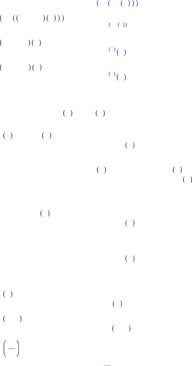
The two curves involved in this problem can be plotted with the implicitplot command from the
plots package. The two solution points can be plotted using plot with style = point. The display
command (also from the plots package) will display the information in both plots in a single plot.
Maple Manual for Fundamentals of Differential Equations, 8e, and Fundamentals of Differential Equations and Boundary Value Problems, 6e.
25
Copyright © 2012 Pearson Education, Inc.
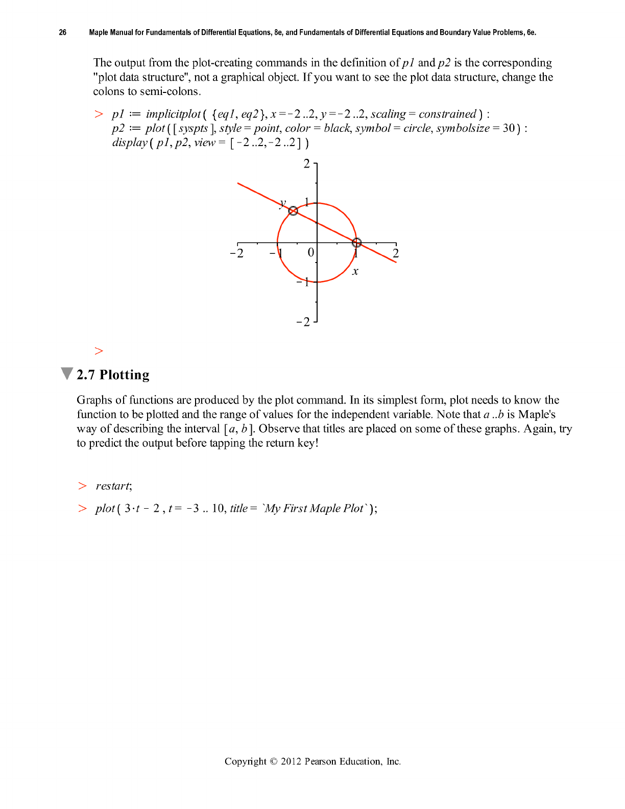
(7.1)(7.1)
O O
O O
(7.2)(7.2)
O O
O O
t
K
2
0
2 4 6 8 10
K
10
10
20
My First Maple Plot
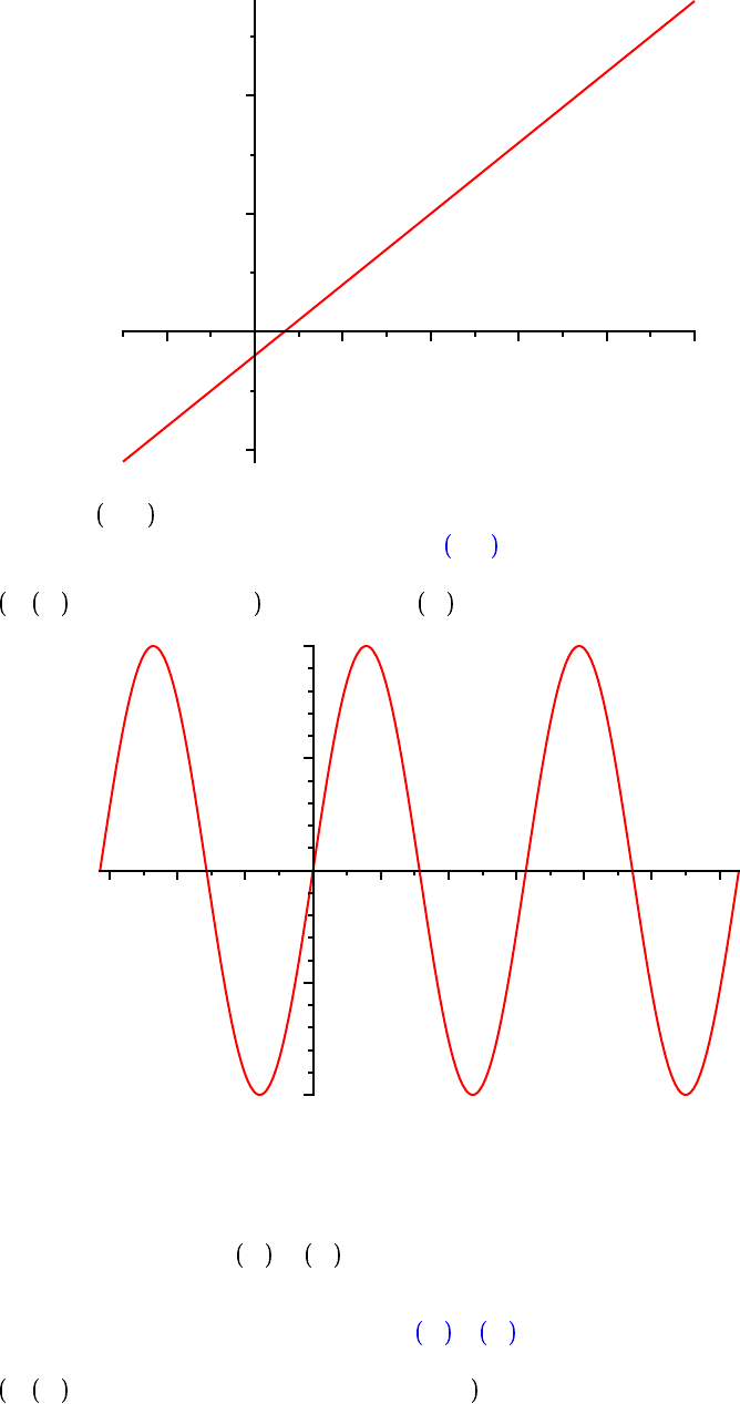
f d x / sin 2$x ;
f := x/sin 2 x
plot f x , x =
K
Pi .. 2$Pi ; #Note that f x is an expression.
x
K
3
K
2
K
1
0
1 2 3 4 5 6
K
1
K
0.5
0.5
1
The preceding command has a remark attached. Everything after the # sign is non-execuable.
g d x/4$x
2
; p d x/f x $g x ;
g := x/4 x
2
p := x/f x g x
plot p x , x =
K
6 .. 8 , title = The product f$g ;
Maple Manual for Fundamentals of Differential Equations, 8e, and Fundamentals of Differential Equations and Boundary Value Problems, 6e.
27
Copyright © 2012 Pearson Education, Inc.
O O
O O
x
K
6
K
4
K
2
0
2 4 6 8
K
100
100
200
The product f*g
These plots are nice, but what information do they convey? Let's concentrate on the plot of f$g, that is,
of p. Position the cursor on a point on the graph and click the left button. The numbers that appear on
the upper-left corner are the coordinates of the current location of the cursor. Use this technique to
identify the global maximum and minimum values of f$g on the interval
K
6, 8 , and the x-values at
which these are found. Where do other (local) minima and maxima occur? Can you guess the exact
values?
plot 2$u
3
C 4$u
K
5 , u =
K
10 .. 7 , title = `cubic function` ;
u
K
10
K
8
K
6
K
4
K
2
0
2 4 6
K
2000
K
1500
K
1000
K
500
500
cubic function
Where does the cubic function cross the u-axis? Maybe it would be helpful to cut down the plotting
interval from
K
10, 7 to
K
1, 3 , or even narrower, say to 0, 1.5 . Try it. Can you find the u-
intercept to 2-decimal point accuracy by this process? It is a powerful method, which we call
Maple Manual for Fundamentals of Differential Equations, 8e, and Fundamentals of Differential Equations and Boundary Value Problems, 6e.
28
Copyright © 2012 Pearson Education, Inc.
O O
O O
O O
(7.3)(7.3)
O O
ZOOMING IN.
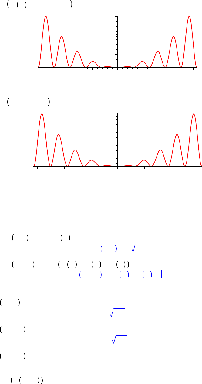
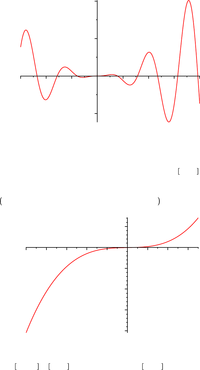
h d x/0.25$cos 8$x ; u1 d x / f x $h x ; u2 d x / f x C h x ;
h := x/0.25 cos 8 x
u1 := x/f x h x
u2 := x/f x C h x
plot u1 x , x =
K
1.2 .. 1.2 ;
x
K
1
K
0.5
0
0.5 1
K
0.2
K
0.1
0.1
0.2
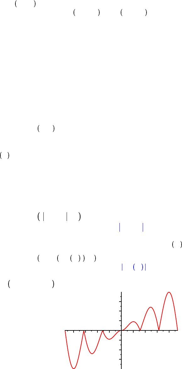
plot u2 x , x = 0 .. 3$Pi ;
x
1 2 3 4 5 6 7 8 9
K
1
K
0.5
0
0.5
1
Maple Manual for Fundamentals of Differential Equations, 8e, and Fundamentals of Differential Equations and Boundary Value Problems, 6e.
29
Copyright © 2012 Pearson Education, Inc.
O O
O O
O O
Can you explain why the graphs of u1 and u2 look the way they do?
You probably now have a big pile of plots cluttering up your screen. Plots can be reduced in size by
putting the cursor on the plot, depressing the mouse key, putting the cursor on one of the dots on the
edge around the graph, and dragging the cursor on the arrow that appears. To permanently get rid of
plots that you no longer need, position the cursor inside the plot window, select with the cursor, and
depress the delete button. Output can also be deleted by highlighting it and selecting the Remove
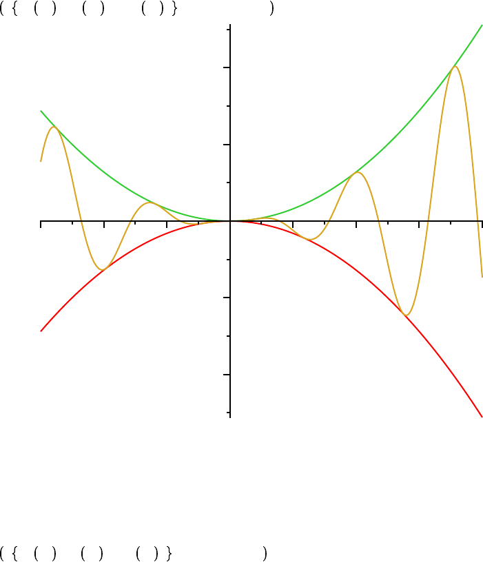
Output under the Edit menu bar.
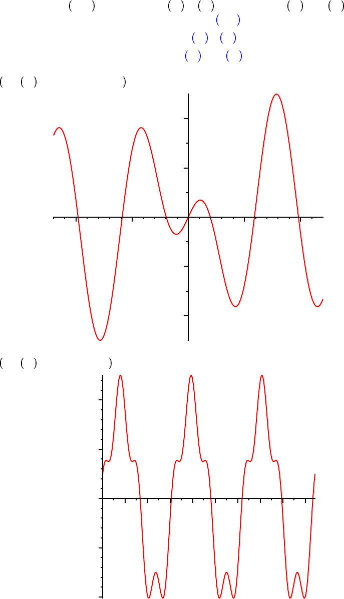
We can also plot many curves simultaneously.
plot p x , g x ,
K
g x , x =
K
6 .. 8 ;
x
K
6
K
4
K
2
0
2 4 6 8
K
200
K
100
100
200
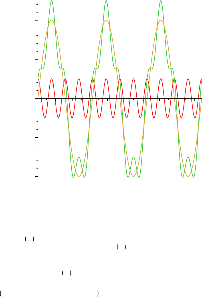
Can you identify the three different plots? What about the next one? Can you explain the little bumps
that appear inside the large dips in the graph of s?
plot f x , h x , u2 x , x = 0 .. 3$Pi ;
Maple Manual for Fundamentals of Differential Equations, 8e, and Fundamentals of Differential Equations and Boundary Value Problems, 6e.
30
Copyright © 2012 Pearson Education, Inc.
O O
O O
(7.4)(7.4)
x
1 2 3 4 5 6 7 8 9
K
1
K
0.5
0
0.5
1
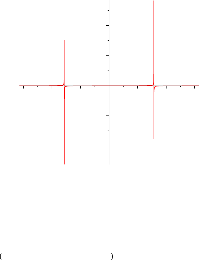
The tangent function is well-known to all of us.
Note: This definition completely replaces the previous definition of f .
f d x/ tan x ;
f := x/tan x
Recall that the graph of y = tan x has vertical asymptotes at all odd multiples of ! / 2. Let's see how
Maple handles this.
plot f ,
K
Pi .. Pi, title = `First Attempt` ;
Maple Manual for Fundamentals of Differential Equations, 8e, and Fundamentals of Differential Equations and Boundary Value Problems, 6e.
31
Copyright © 2012 Pearson Education, Inc.
O O
K
3
K
2
K
1
0
1 2 3
K
2000
K
1000
1000
2000
First Attempt
Is this what you expected to see? Why does the graph look like this? What can be done to improve the
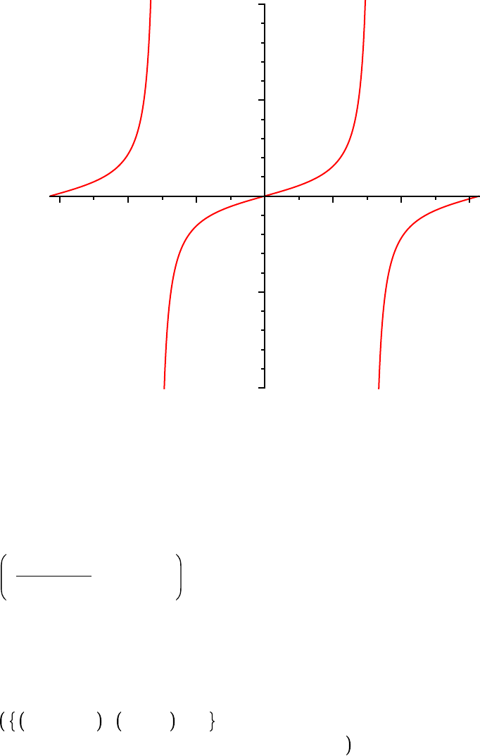
appearance of the plot?
There are two problems. First, we have to tell Maple that this function is discontinuous. But, there is
more. Look at the labels on the vertical axis. The units are VERY LARGE on the y-axis; we want to
see the details on a much finer scale. Let's limit the vertical scale in the range from -10 to 10. Each of
these pieces of information is an optional argument to plot.
plot f,
K
Pi .. Pi ,
K
10 .. 10 , discont = true ;
Maple Manual for Fundamentals of Differential Equations, 8e, and Fundamentals of Differential Equations and Boundary Value Problems, 6e.
32
Copyright © 2012 Pearson Education, Inc.
O O
O O
K
3
K
2
K
1
0
1 2 3
K
10
K
5
5
10
This technique is very useful for any function that has vertical asymptotes.
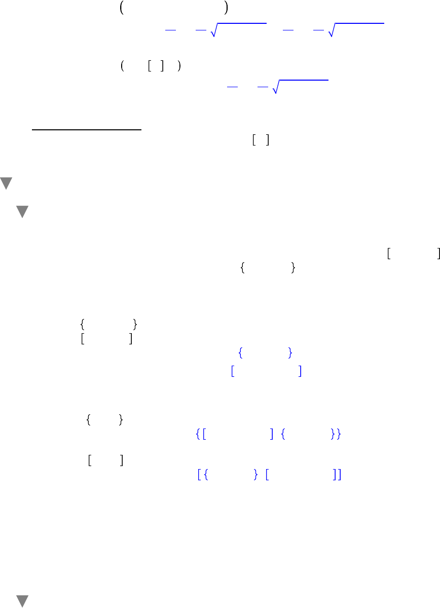
OK. Now it's your turn. Add appropriate optional arguments to the following command to produce a
graph from which you can identify the local minimum and local maximum. (Don't forget the title.)
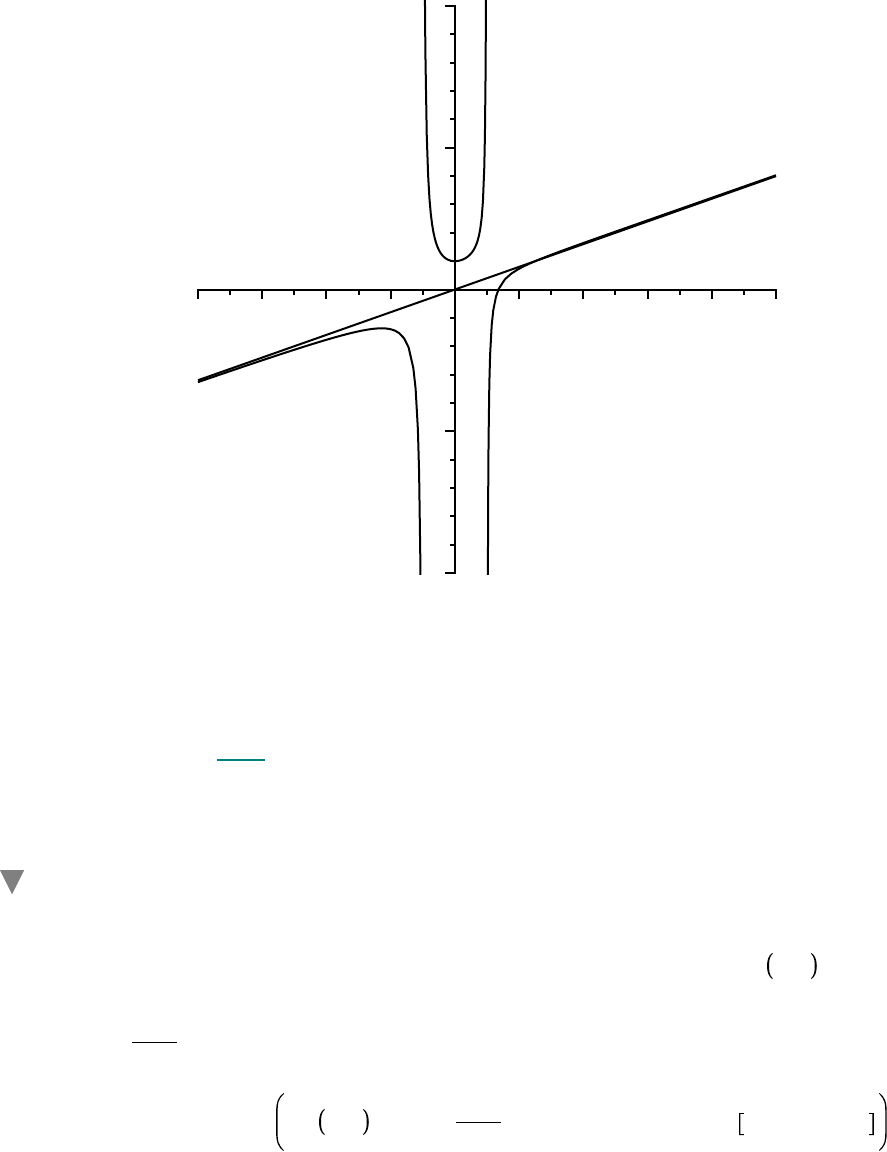
plot
10
K
4$t
3
1
K
t
2
, t =
K
3 .. 5 ;
Now, one last challenge. Use your graph to estimate the (oblique) asymptote for this function. Check
your estimate by graphing the function and the asymptote in the same plot. (Here's an example of what
we are seeking, and to show how plots look when inserted into a worksheet.)
plot 10
K
4$t
3
/ 1
K
t
2
, 4$t , t =
K
8 ..10,
K
100 ..100, discont = true, color = black, title
= `Discontinous Function with Oblique Asymptote` ;
Maple Manual for Fundamentals of Differential Equations, 8e, and Fundamentals of Differential Equations and Boundary Value Problems, 6e.
33
Copyright © 2012 Pearson Education, Inc.
O O
O O
O O
K
8
K
6
K
4
K
2
0
2 4 6 8 10
K
100
K
50
50
100
Discontinous Function with Oblique Asymptote
These examples only scratch the surface of Maple's abilities when it comes to plotting. Maple can also
produce 3-D plots, plots of parametric curves and surfaces, and animated sequences. We will examine
some of these in the next section about Maple packages. The best general source of information is the
on-line help for the plots package.
?plots;
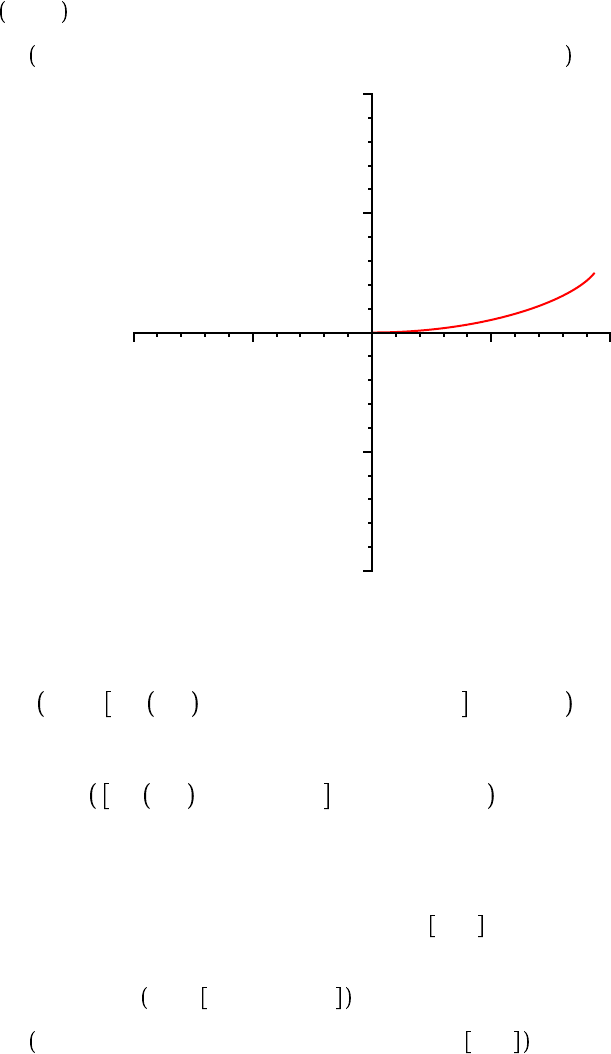
2.8 Creating Animations
One way to make a Maple animation is to form a sequence of Maple plots and use display to show
them in sequence. For example, to animate the drawing of the function r = sin 5 " for 0 ! " ! ! in
polar coordinates first create a sequence of plots of the function over shorter time intervals, say
0 ! " !
n$!
12
, for n = 1 ..12 .
polarframes d'plot sin 5 " , " = 0 ..
n$!
12
, coords = polar, view =
K
1 ..1,
K
1 ..1 '
$ n = 1 ..12 :
The display command from the plots package will display the plots in sequence if the optional equation
insequence = true is used. The animation is, of course, playable only in an active Maple worksheet (or
a worksheet that has been exported to HTML). To play the animation, click the first frame of the
output. Then use the control buttons that appear on the Context Bar to advance through the frames
Maple Manual for Fundamentals of Differential Equations, 8e, and Fundamentals of Differential Equations and Boundary Value Problems, 6e.
34
Copyright © 2012 Pearson Education, Inc.
O O
O O
O O
O O
O O
O O
individually, once from beginning to end, or continuously.
with plots :
display polarframes, insequence = true, scaling = constrained
K
1
K
0.5
0
0.5 1
K
1
K
0.5
0.5
1
The plots package has a two procedures: animate and animatecurve, that will automatically create this
sort of animation. The code for animate is shown below.
animate plot, sin 5 " , " = 0 ..T, coords = polar , T = 0 ..! :
The code using animatecurve is shown next. See the Help pages for animate and animatecurve.
animatecurve sin 5 " , ", " = 0 .. ! , coords = polar :
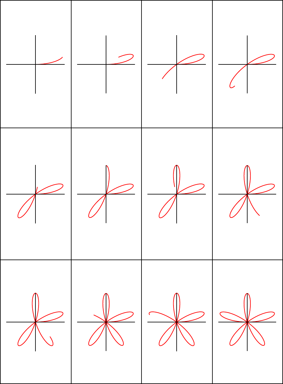
For a hardcopy such as this, it makes more sense to create the first animation and then display all 12
frames as an array (Matrix in Maple) with three rows, each containing four plots. The Matrix command
is used to create the 3 # 4 array of the plots named polarframes, then the display command is used to
display the result. The optional argument tickmarks = 0, 0 suppresses the tickmarks on both axes
(they become too cluttered to be of any use).
Frames d Matrix 3, 4, polarframes :
display Frames, scaling = constrained, tickmarks = 0, 0
Maple Manual for Fundamentals of Differential Equations, 8e, and Fundamentals of Differential Equations and Boundary Value Problems, 6e.
35
Copyright © 2012 Pearson Education, Inc.
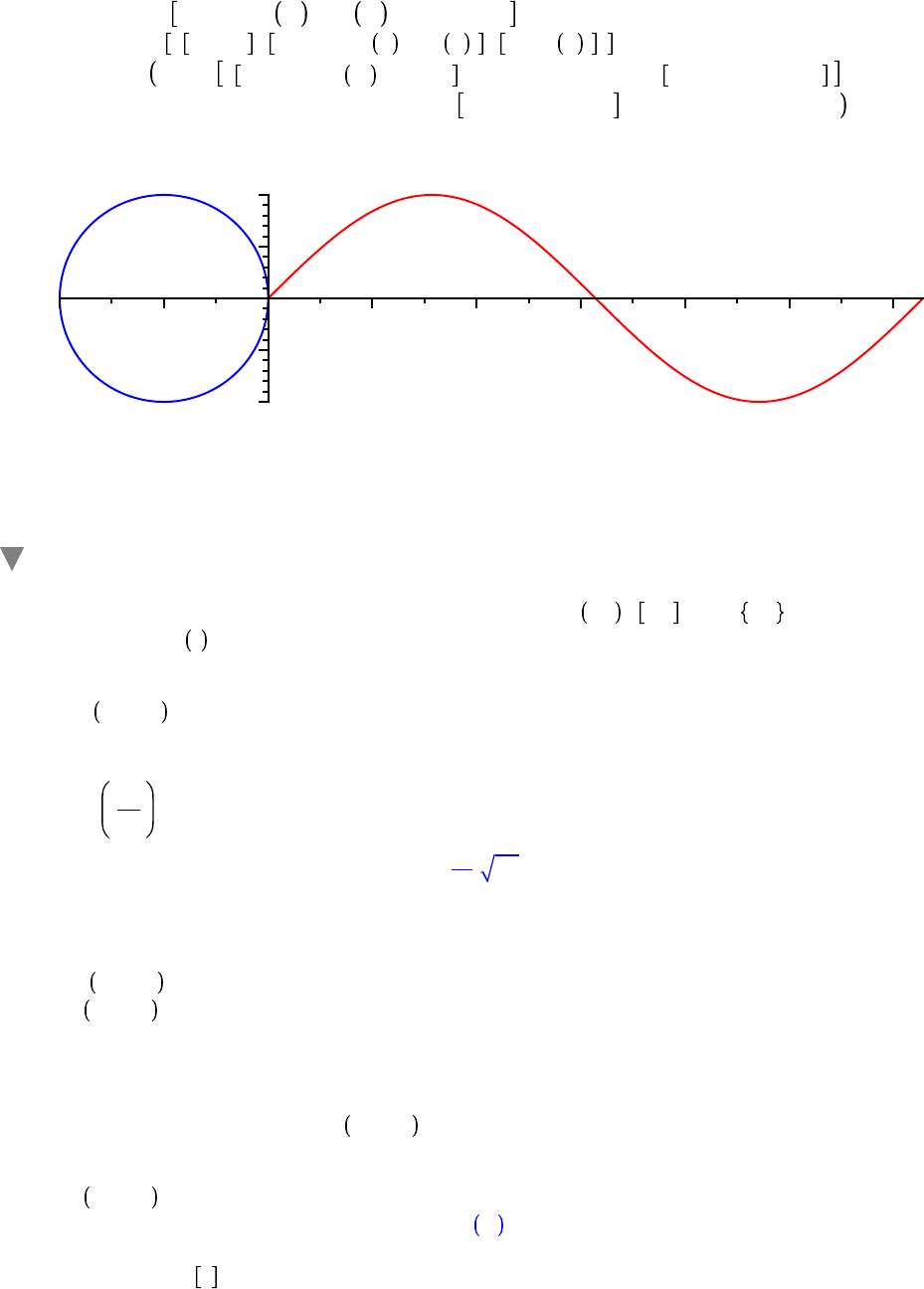
The concluding example in this section illustrates the relationship between the unit circle and the sine
curve. The idea is to animate a point moving around a unit circle with lines tracing out a sine curve. The
command is a bit involved but once you see the animation and look at the pieces used to compose the
Maple Manual for Fundamentals of Differential Equations, 8e, and Fundamentals of Differential Equations and Boundary Value Problems, 6e.
36
Copyright © 2012 Pearson Education, Inc.
O O
(9.4)(9.4)
(9.2)(9.2)
O O
O O
O O
(9.3)(9.3)
O O
(9.1)(9.1)
O O
individual frames, the input will become much less mysterious. The animate procedure is used.
Circle d
K
1 C cos " , sin " , " = 0 ..2 ! :
Lines d
K
1, 0 ,
K
1 C cos t , sin t , t, sin t :
animate plot, Circle, sin x , Lines , x = 0 ..2 !, color = blue, red, black ,
t = 0 ..2 !, view =
K
2 ..2 !,
K
1 ..1 , scaling = constrained
x
K
2
K
1 1 2 3 4 5 6
K
1
K
0.5
0.5
1
t = 0.
2.9 Three Types of Brackets in Maple
Three types of brackets have been used in this worksheet: ... , ... , and ... . Parentheses, or
round brackets, , are used for the mathematical grouping of terms, including the specification of
function arguments.
7$ 3 C 1
28
sin
!
4
1
2
2
The multiplication symbol in the first example can also be indicated with a space, or not.
7 3 C 1 ;
7 3 C 1
28
28
However, an entry of the form x 3 C 1 will be interpreted as the function named x applied to the
argument 3 C 1.
x 3 C 1
x 4
Square brackets, , are used for creating lists and accessing elements in lists, arrays, matrices, and
Maple Manual for Fundamentals of Differential Equations, 8e, and Fundamentals of Differential Equations and Boundary Value Problems, 6e.
37
Copyright © 2012 Pearson Education, Inc.
O O
O O
(9.5)(9.5)
(9.8)(9.8)
O O
(9.12)(9.12)
(9.6)(9.6)
O O
(9.11)(9.11)
O O
O O
O O
(9.7)(9.7)
(9.9)(9.9)
(9.10)(9.10)
O O
O O
tables.
List d 2, 3, 3, 2 ;
List 3 ..4
List := 2, 3, 3, 2
3, 2
Square brackets can also be used to create a table to store data. If b is a free variable, then the entry
b 3 d 7
b
3
:= 7
causes Maple to create a place in its memory for a table named "b" and to store in this table the number
7, indexed by the number 3. The next entry
b cow d cos
b
cow
:= cos
stores the cosine function in the table b, indexed by the variable cow. The index for a tabular entry can
be anything that makes sense to Maple (cow is just another variable, as far as Maple is concerned).
We can even store in b the variable cow, indexed by the cosine function
b cos d cow
b
cos
:= cow
and then ask Maple to evaluate a silly entry like this
b cow b cos $b 3
cos 7 cow
or another silly entry like this
b cos b cow 3
cow cos 3
Enter print b to see what is stored in the table.
print b
table 3 = 7, cow = cos, cos = cow
A restart clears all of this from memory. Tables can be very useful; enter ?table to see the Help page
for table.
restart
Curly brackets, , are used for creating sets.
n
2
$ n =
K
2 ..2
0, 1, 4
Do not attempt to interchange these symbols! Nothing good will happen.
Maple Manual for Fundamentals of Differential Equations, 8e, and Fundamentals of Differential Equations and Boundary Value Problems, 6e.
38
Copyright © 2012 Pearson Education, Inc.
O O
(10.1.2)(10.1.2)
O O
O O
O O
O O
O O
O O
O O
O O
O O
(10.1.3)(10.1.3)
(9.14)(9.14)
(10.1.1)(10.1.1)
(10.2.1)(10.2.1)
O O
(9.13)(9.13)
sin
!
4
sin
1
4
!
sin !
sin !
2.10 Common Problems and How to Fix Them
Using a Command Before It Is Loaded Into the Maple Kernel
Some commands are defined as part of a package that is not automatically loaded into the Maple
kernel. If one of these commands is used prior to loading the package, the output will simply echo
the input after the arguments have been simplified (if possible). For example,
restart
CompleteSquare x
2
C 2 x C 2
CompleteSquare x
2
C 2 x C 2
with Student Precalculus
CenterOfMass, CompleteSquare, CompositionPlot, CompositionTutor, ConicsTutor,
Distance, FunctionSlopePlot, FunctionSlopeTutor, LimitPlot, LimitTutor, Line,
LineTutor, LinearInequalitiesTutor, Midpoint, PolynomialTutor,
RationalFunctionPlot, RationalFunctionTutor, Slope, StandardFunctionsTutor
CompleteSquare x
2
C 2 x C 2
x C 1
2
C 1
Using Reserved Words and Protected Names
Maple places relatively few restrictions on the names that can be used for objects. When such a
name is used, Maple generates an appropriate error message.
D d 7
Error, attempting to assign to `D` which is protected
Maple reserves D for the differentiation operator.
D x/x sin x
x/sin x C x cos x
! d 3.14
Error, attempting to assign to `Pi` which is protected
Maple Manual for Fundamentals of Differential Equations, 8e, and Fundamentals of Differential Equations and Boundary Value Problems, 6e.
39
Copyright © 2012 Pearson Education, Inc.
O O
O O
O O
O O
uniond 1, 2, 3
Error, invalid union
uniond 1, 2, 3
Be forewarned, however, that if a value is assigned to a name that is also a Maple command, then
the new assignment overwrites the command definition. This feature can be used to extend or
customize the functionality of some of Maple's built-in commands.
2.11 Programming with Maple
There are basically three aspects of programming in Maple that we will be using in this manual. They
are the use of repetitive loops (for loops), the use of conditionals (if - then), and procedures.
Let's begin with repetitive loops since they may be used in procedures
The general syntax for the simplest form of a repetitive loop is as follows:
for <name> from <initial_value> by <value> to <end_value>
do
<statement_sequence>
od;
or,
for <name> from <initial_value> by <value> while <relation>
do
<statement_sequence>
od;
where the loop must be terminated by od; or equivalently od: and the expression "by <value>" is
optional where Maple increments by +1 if this is omitted. Consider as an example of a repetitive loop
which outputs 1, 2 and 3 all raised to the 4th power.
The repetitive loop would begin as,
for n from 1 to 3
Error, unterminated for loop
for n from 1 to 3
Since the first line of this program does not merit a semi(colon), Maple responds with a warning and a
new line of input. The warning statement(s) disappear when the program is valid, complete and closed
by a semi(colon). Our repetitive loop and output could be in either of the following forms.
Maple Manual for Fundamentals of Differential Equations, 8e, and Fundamentals of Differential Equations and Boundary Value Problems, 6e.
40

Copyright © 2012 Pearson Education, Inc.
O O
O O
(11.1)(11.1)
O O
O O
(11.2)(11.2)
O O
for n from 1 to 3 do n
4
od;
1
16
81
for n from 1 by 1 while n ! 4 do n
4
od;
1
16
81
Additional lines can be inserted within an execution group by placing the cursor just left of the new line
operator > and hitting enter. Or, the execution group can be split at the present cursor location by
selecting Split or Join from the Edit pull-down menu. Separated execution groups can be joined two
at a time by highlighting neighbor execution groups and selecting Split or Join from the Edit menu
and then selecting Join Execution Groups.
The general syntax for a selection statement is as follows:
if <relation>
then <statement_sequence>
elif <relation>
then <statement_sequence>
.....
elif <relation>
then <statement_sequence>
else <statement_sequence>
fi;
where the if-statement must be terminated by either fi; or fi:, elif ("else if") and else are optional, and
there can be as many "else if" statements as desired.
As an example of the use of a selection statement, lets pick 1000 random numbers between 0 and 2. We
will say the number is good if it is less than one. We will multiply all those between 0 and 1 together
and keep a record of how many between 0 and 1 are selected. We will use the random number
generator of Maple to select the random number.
restart;
ran_num d rand 0 ..1000 / 500.0 :
Maple Manual for Fundamentals of Differential Equations, 8e, and Fundamentals of Differential Equations and Boundary Value Problems, 6e.
41
Copyright © 2012 Pearson Education, Inc.
(11.3)(11.3)
(11.4)(11.4)
O O
O O
O O
O O
O O
O O
O O
Let's see some of the random number generated by this procedure.
for n from 1 to 5 do lprint ran_num od;
1.720000000
1.516000000
1.500000000
1.778000000
.6000000000
good d 0 : bad d 0 : prod d 1 :
for n from 1 to 100 do x d ran_num : if x ! 1 then good d good C 1 : prod
d prod$x : else bad d bad C 1 : fi: od:
lprint `less_than_one=`, good, `product=`, prod ; `less_than_one=`, 50, `product=`,
.1003899574e-23
`less_than_one=`, 57, `product=`, 0.1519492198e-25
less_than_one=, 50, product=, 1.003899574 10
-24
Note that the product is very small as it should be. You can try 1000 numbers and see what product
becomes and see if 1/2 of the numbers chosen are between 0 and 1.
restart;
Finally let's examine procedures. We can combine several activities together and call it a procedure.
Then whenever we wish to use it we just have to call for it. The general syntax of a Maple procedure is
as follows,
procedure_name:=proc(input_variables)
<statement_sequence>
<statement_sequence>
.....
<statement_sequence>
end;
where all procedures must be terminated by end; or end:. A function is an example of a procedure. We
can program the function f x = x
2
as a procedure as follows,
f dproc x x
2
end;
f := proc x x^ 2 end proc
If the procedure is valid and closed by a semicolon, then pressing enter activates Maple to display the
program in a blue color while ending the procedure with a colon hides a re-display of the program
Maple Manual for Fundamentals of Differential Equations, 8e, and Fundamentals of Differential Equations and Boundary Value Problems, 6e.
42
Copyright © 2012 Pearson Education, Inc.
O O
O O
O O
O O
O O
O O
(11.6)(11.6)
(11.7)(11.7)
(11.5)(11.5)
O O
O O
code. A procedure can then be invoked by name, in this case f, as demonstrated below.
f 2 , f 4 , f a , f b , f a C b ;
4, 16, a
2
, b
2
, a C b
2
In constructing more complicated procedures, it is often useful to declare the scope of the variables
used. A local variable is active only within the execution group where it is declared while a variable
declared global retains its value for the entire worksheet. Consider this distinction within the following
procedure which computes the sum of square integers from 1 to 3.
sum_of_square d proc global total;local n; total d 0 : for n from 1 to 3 do total
d total C n^ 2 od: lprint `Procedure Complete` ; end:
We invoke this procedure by name,
sum_of_square ;
`Procedure Complete`
The incremental variable n was declared local by the programmer. In comparison, the variable total
was declared global. Because of this distinction, total retains its value outside of this procedure, while
variable n does not.
print total, n ;
14, n
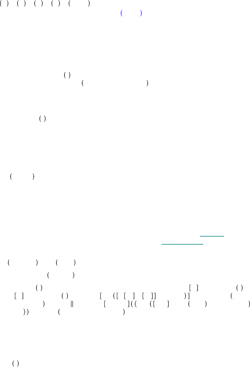
Another application of procedures are animations. Imagine throwing darts at random onto a unit
square. Inside the square is one fourth of the unit circle with the radius on two sides of the square. We
can animate this process by plotting the random data values within the unit square in the first quadrant
some of which will land within the unit circle (where arc() is located within the plottools library) and
storing plots in sequence as single frames of an animation via the dot (.) operator. The frames are
implicitly declared global; all other variables used within this procedure can be declared local.
with plottools : with plots :
ran_num d rand 0 ..1000 / 1000.0 :
Darts dproc local x, y, n, m, table, data; for n from 1 to 75 do x n d ran_num :
y n d ran_num : table d seq x m , y m , m = 1 ..n : data d plot table,
style = point : frames n d plots display arc 0, 0 , 1, 0 .. Pi/ 2 , color = black ,
data ; od; print `Procedure Complete` ; end:
This procedure is run by name, and the frames of the animation are compiled by the display command,
where insequence=false places all frames of an animation on top of one another, while insequence=
true retains frame sequencing.
Darts ;
Procedure Complete
Maple Manual for Fundamentals of Differential Equations, 8e, and Fundamentals of Differential Equations and Boundary Value Problems, 6e.
43

Copyright © 2012 Pearson Education, Inc.
4. 4.
1. 1.
2. 2.
2. Introduction to Maple, Part 2
Document Mode
Interaction with Maple takes place one of two modes: the default Worksheet Mode or Document Mode.
Part 1 of this Introduction to Maple discusses Worksheet Mode. This part describes Document Mode. It is
assumed that the reader is familiar with the topics discussed in Part 1 and has experience working in
Worksheet Mode.
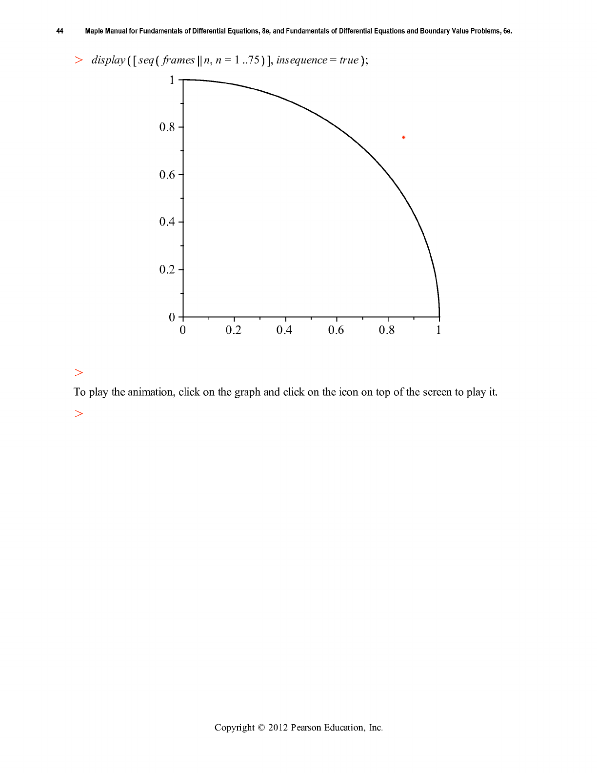
2.12 Document Mode vs Worksheet Mode
Worksheet Mode is characterized by a strict separation between text and executable mathematics.
Mathematics input for execution is typed at an input prompt (in what is called an Execution Group) and
text is typed in a Text Group.
In Document Mode the user begins with a blank page. There are no input prompts. One toggles
between text and mathematics by pressing the [F5] key or [control-T] for text and [control-R] for
mathematics. The latter is our choice because it is a bit faster.
For Macintosh users,the [command] key (the key with the apple symbol)
is used instead of [control].
Mathematics entries are made in the 2D input style as described in Part 1. Math entries can be made
simply to be read, or they can be sent to Maple for processing (i.e. "evaluated") in one of three ways:
Click on a math entry and press [control-equals] for an in-line evaluation. The input is processed
and the output appears in the same line.
Click on a math entry and press the [enter] key. In this case, the entry is processed and the output
appears centered on the next line (with a label).
Right-Click on a math entry, usually an expression of some sort. This calls a contextual menu
with a list of procedures and commands that are suitable for that particular expression. Choose the
one that is desired and it will be applied. The output appears in-line. (Macintosh users with a one-
button mouse will do a [control-click].)
2.13 Examples
In-Line Evaluation
This is Maple, in Document Mode, and this is an in-line evaluation,
d
dx
2
x
= 2
x
ln 2 . So is the
next line.
0
4
x
x
4
C 2
dx =
1
4
arctan 8 2 2 .
The integral is centered for the sake of appearance.
Maple Manual for Fundamentals of Differential Equations, 8e, and Fundamentals of Differential Equations and Boundary Value Problems, 6e.
45
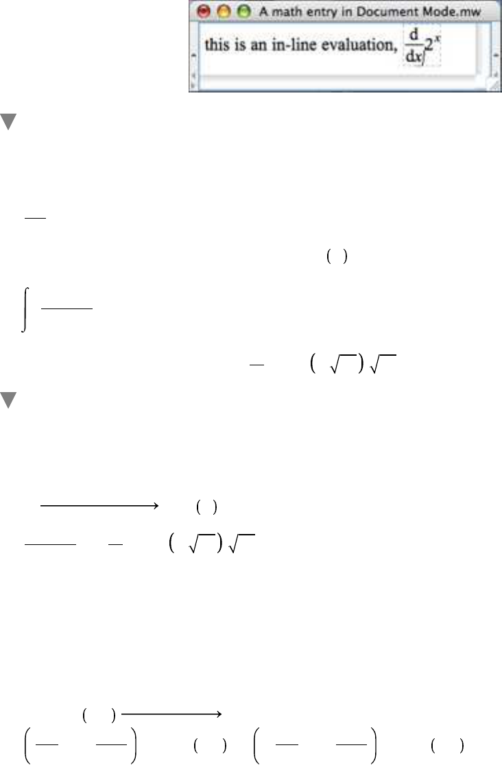
Copyright © 2012 Pearson Education, Inc.
(2.2.1)(2.2.1)
(2.2.2)(2.2.2)
Each expression was entered in math mode ([control-R]) and [control-equals] was pressed for
evaluation ([command-equals] on a Mac). After evaluation, [control-T] puts Maple back into text
mode. When Maple is in text mode the word Text is highlighted in the Context Bar. When in math
mode the word Math is highlighted and the input cursor is slanted to the right. Moreover, the entire
math entry is enclosed in a rectangular box that expands as terms are entered. A screen shot is
shown below.
Traditional Evaluation
The following calculations were made in the traditional way, by pressing the [enter] key. The
output is on the next line, centered, and with a label, as it would be in Worksheet Mode.
d
dx
2
x
2
x
ln 2
0
4
x
x
4
C 2
dx
1
4
arctan 8 2 2
Contextual Menu Evaluation
The following evaluations were made using contextual menus. Note that only the expression has
been entered. The operation or procedure that is applied to the expression is chosen from a
contextual menu which varies according to the type of expression that is selected.
2
x
differentiate w.r.t. x
2
x
ln 2
x
x
4
C 2
/
1
4
arctan 8 2 2
The derivative calculation was made by choosing "Differentiate" then "x" on a pop-out menu. For
the the definite integral calculation "Apply a Command" was chosen. Then "int" and "x=0..4" were
entered in the two fields in the ensuing dialogue.
Here are four more examples.
Choose "Integrate" to obtain the antiderivative of an expression.
x e
2 x
cos 3 x
integrate w.r.t. x
2
13
x C
5
169
e
2 x
cos 3 x
K
K
3
13
x C
12
169
e
2 x
sin 3 x
The general solution to a second order differential equation is obtained by choosing "Solve DE".
Maple Manual for Fundamentals of Differential Equations, 8e, and Fundamentals of Differential Equations and Boundary Value Problems, 6e.
46
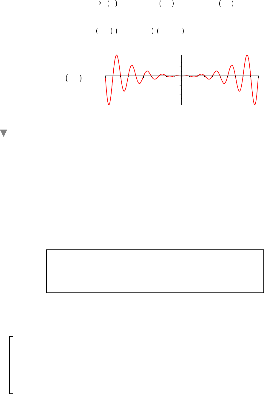
Copyright © 2012 Pearson Education, Inc.
y''C 2 y'C 5 y = 0
solve DE
y x = _C1 e
K
x
sin 2 x C _C2 e
K
x
cos 2 x
Choose "Integer Factors" to factor an integer.
12345678910111213 =
factor
113 869211457 125693
Choose "Plot" to obtain the graph of an expression.
0.1 x e
K
0.2 x
sin ! x /
K
10
K
5 5 10
K
6
K
4
K
2
2
4
The default horizontal range for a contextual menu plot is from
K
10 to 10.
2.14 Why Document Mode?
Document Mode can be used to produce professional-looking technical documents that mix text,
mathematics to be read, and processed mathematics (plots, evaluations, approximations, ... ). Printed
documents are of excellent quality. Flexibility with the layout of a document is facilitated by the use of
tables that are inserted from the Insert Menu and managed from the Table Menu. See the next
section.
New Maple users, freed from the apparatus of Execution Groups, input prompts, and output regions,
may take advantage of contextual menus to apply a command or a procedure without prior knowledge
of either its name or its syntax. Those who want to learn the names and the syntax of the procedures
can right-click on an expression that has been entered at an input prompt.
"An input prompt?" you ask; well, "Yes."
Switch to Worksheet Mode
Worksheets that begin in Document Mode can be converted to Worksheet
Mode by inserting an Execution Group from the Insert Menu (or by
pressing [control-J]R[command-J] on a Mac).
The following Worksheet-style entries were made by pressing [command-J]. Note the left brackets
that enclose each type of entry...Text Group and Execution Group. This is the sign that Maple is in
Worksheet Mode.
While in Worksheet Mode, a right-click on an executable math expression (i.e. one that is at an input
prompt) will call a contextual menu. But then, as soon as an appropriate procedure is chosen, Maple
enters another Execution Group whose input is the procedure that accomplishes the specified
operation. The procedure is then processed automatically.
For example, the contextual menu derivative evaluation made earlier looks like this in Worksheet
Mode,
Maple Manual for Fundamentals of Differential Equations, 8e, and Fundamentals of Differential Equations and Boundary Value Problems, 6e.
47
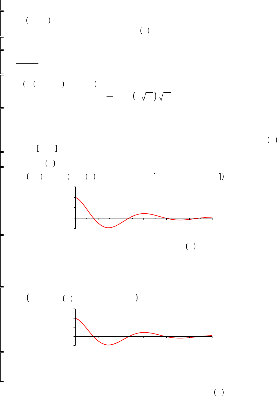
Copyright © 2012 Pearson Education, Inc.
O O
O O
O O
O O
(3.2)(3.2)
O O
(3.1)(3.1)
O O
O O
2
x
diff 2^ x, x
2
x
ln 2
and the definite integral calculation looks like this.
x
x
4
C 2
int x / x^ 4 C 2 , x = 0 .. 4
1
4
arctan 8 2 2
Observe that the procedures that Maple inserted are written in the 1D input style. So, not only are the
calculations made, but the associated procedures are displayed in explicit "typewriter" syntax.
In the next example, a contextual menu evaluation is used to graph the expression e
K
0.25 x
cos x over
the interval 0, 12 .
e
K
0.25 x
cos x
plot exp
K
.25 * x * cos x , x = 0 .. 12, view = DEFAULT,
K
.5 .. 1.5
2 4 6 8 10 12
K
0.5
0
0.5
1
1.5
This particular plot was obtained by right-clicking on e
K
0.25 x
cos x and choosing "Plots/Plot
Builder" on the contextual menu. The ensuing dialogue gives full control over the appearance of the
plot. The horizontal and vertical plot ranges were set only after experimenting with some trial plots
which were provided by the Plot Builder dialogue.
As shown below, the view option in the plot input can be simplified somewhat.
plot e
K
0.25 x
cos x , x = 0 ..12,
K
0.5 ..1.5
2 4 6 8 10 12
K
0.5
0
0.5
1
1.5
Upon the insertion of one Execution Group, all subsequent entries in the worksheet are in Worksheet
Mode, i.e. with input prompts for the executable math entries. To return to Document Mode, choose
Create Document Block on the Format Menu.
Once back into Document Mode, a right-click on the expression e
K
0.25 x
cos x produces a plot output
that looks like this (Plot Builder called again).
Maple Manual for Fundamentals of Differential Equations, 8e, and Fundamentals of Differential Equations and Boundary Value Problems, 6e.
48
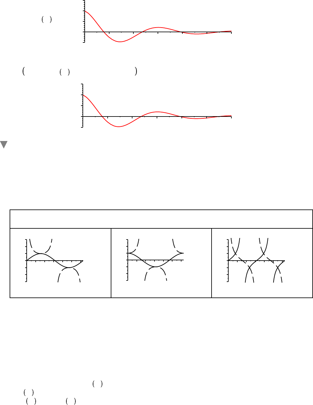
Copyright © 2012 Pearson Education, Inc.
e
K
0.25 x
cos x /
2 4 6 8 10 12
K
0.5
0
0.5
1
1.5
Direct application of the plot procedure looks like this.
plot e
K
0.25 x
cos x , x = 0 ..12,
K
0.5 ..1.5
2 4 6 8 10 12
K
0.5
0
0.5
1
1.5
2.15 Tables
Ease of entry and manipulation make tables a useful formatting tool for the creation of publishable
documents. This section provides three examples.
The display below was initially a two row three column "table" obtained by choosing Table... on the
Insert Menu.
The Six Trigonometric Functions, Two at a Time
1 2 3 4 5 6
K
3
K
2
K
1
0
1
2
3
sine and cosecant
1 2 3 4 5 6
K
3
K
2
K
1
0
1
2
3
cosine and secant
1 2 3 4 5 6
K
3
K
2
K
1
0
1
2
3
tangent and cotangent
The three columns in the first row were merged using a selection on the Tables Menu. After each cell
was filled (text and plots) the Properties... dialogue (Tables Menu) was used to hide the plot inputs in
the three cells containing the plots.
The same Properties... dialogue can be used to hide the lines separating tabular cells. This is how the
following display was created, starting with a table with one row and three columns.
The plots on the right show the
essential differences between the
trigonometric functions sin x
and
cos x
and the hyperbolic functions
sinh x
and cosh x when x is small.
Examine their Taylor series
Maple Manual for Fundamentals of Differential Equations, 8e, and Fundamentals of Differential Equations and Boundary Value Problems, 6e.
49
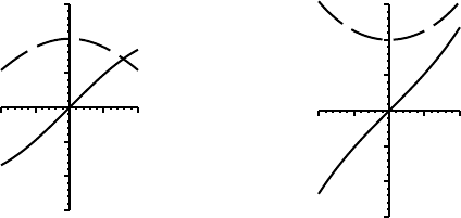
Copyright © 2012 Pearson Education, Inc.
expansions to see why, for even
smaller x, the differences would be
negligible.
K
1 0.5 1
K
1.5
K
1
K
0.5
0.5
1
1.5
sine and cosine
K
1 0.5 1
K
1.5
K
1
K
0.5
0.5
1
1.5
sinh and cosh
The last example is a short table of Laplace transform properties. They are included to illustrate the
quality of math entries that are made strictly to be read.
Maple Manual for Fundamentals of Differential Equations, 8e, and Fundamentals of Differential Equations and Boundary Value Problems, 6e.
50
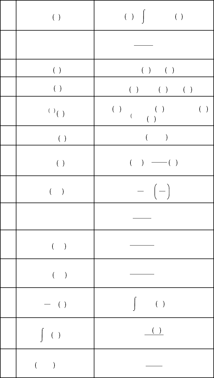
Copyright © 2012 Pearson Education, Inc.
The Laplace Transform
f t
F s =
0
CN
e
s$t
$f t dt
0.
t
n
, n = 0, 1, 2, ...
n!
s
n C 1
, s O 0
1.
f ' t
s$F s
K
f 0
2.
f '' t
s
2
$F s
K
s$f 0
K
f ' 0
3.
f
n
t
s
n
$F s
K
s
n
K
1
$f 0
K
s
n
K
2
$f ' 0
K
...
K
f
n
K
1
0
4.
e
a$t
f t
F s
K
a
5.
t
n
$f t
K
1
n
$
d
n
F
ds
n
s
6.
f a$t
1
a
$F
s
a
7.
e
a$t
1
s
K
a
, s O a
8.
sin b$t
b
s
2
C b
2
, s O 0
9.
cos b$t
s
s
2
C b
2
, s O 0
10.
1
t
$f t
s
CN
F u du
11.
0
t
f v dv
F s
s
12.
u t
K
a , a R 0
e
K
a$s
s
Maple Manual for Fundamentals of Differential Equations, 8e, and Fundamentals of Differential Equations and Boundary Value Problems, 6e.
51
Copyright © 2012 Pearson Education, Inc.
13.
" t
K
a , a R 0
e
K
a$s
14.
f t
K
a $u t
K
a , a
R 0
e
K
a$s
$F s
15. f)g t F s $G s
Maple Manual for Fundamentals of Differential Equations, 8e, and Fundamentals of Differential Equations and Boundary Value Problems, 6e.
52
