Journal of Machine Learning Research 13 (2012) 2617-2654 Submitted 8/11; Revised 5/12; Published 9/12
Static Prediction Games for Adversarial Learning Problems
Michael Br
¨
uckner MIBRUECK@CS.UNI-POTSDAM.DE
Department of Computer Science
University of Potsdam
August-Bebel-Str. 89
14482 Potsdam, Germany
Christian Kanzow KANZOW@MATHEMATIK.UNI-WUERZBURG.DE
Institute of Mathematics
University of W
¨
urzburg
Emil-Fischer-Str. 30
97074 W
¨
urzburg, Germany
Tobias Scheffer SCHEFFER@CS.UNI-POTSDAM.DE
Department of Computer Science
University of Potsdam
August-Bebel-Str. 89
14482 Potsdam, Germany
Editor: Nicol
`
o Cesa-Bianchi
Abstract
The standard ass umption of identically distributed training and test data is violated when the test
data are generated in response to the presence of a predictive model. This becomes apparent, for
example, in the context of email spam filtering. Here, email service providers employ spam fil-
ters, and spam senders engineer campaign templates to achieve a high rate of successful deliveries
despite the filters. We model the interaction between the learner and the data generator as a static
game in which the cost functions of the learner and the data generator are not necessarily antag-
onistic. We identify conditions under which this prediction game has a unique Nash equilibrium
and derive algorithms that find the equilibrial prediction model. We derive two instances, the Nash
logistic regression and the Nash support vector machine, and empirically explore their properties
in a case study on email spam filtering.
Keywords: static prediction games, adversarial classification, Nash equilibrium
1. Introduction
A common assumption on which most learning algorithms are based is that training and test data
are governed by identical distributions. However, in a variety of applications, the distribution that
governs data at application time may be influenced by an adversary whose interests are in conflict
with those of the learner. Consider, for instance, the following three scenarios. In computer and
network security, scripts that control attacks are engineered with botnet and intrusion detection
systems in mind. Credit card defrauders adapt their unauthorized use of credit cards—in particular,
amounts charged per transactions and per day and the type of businesses that amounts are charged
from—to avoid triggering alerting mechanisms employed by credit card companies. Email spam
senders design message templates that are instantiated by nodes of botnets. These templates are
c
2012 Michael Br
¨
uckner, Christian Kanzow and Tobias Scheffer.
BR
¨
UCKNER, KANZOW, AND SCHEFFER
specifically designed to produce a low spam score with popular spam filters. The domain of email
spam filtering will serve as a running example throughout the paper. In all of these applications, the
party that creates the predictive model and the adversarial party that generates future data are aware
of each other, and factor the possible actions of their opponent into their decisions.
The interaction between learner and data generators can be modeled as a game in which one
player controls the predictive model whereas another exercises some control over the process of
data generation. The adversary’s influence on the generation of the data can be formally modeled as
a transformation that is imposed on the distribution that governs the data at training time. The trans-
formed distribution then governs the data at application time. The optimization criterion of either
player takes as arguments both the predictive model chosen by the learner and the transformation
carried out by the adversary.
Typically, this problem is modeled under the worst-case assumption that the adversary desires
to impose the highest possible costs on the learner. This amounts to a zero-sum game in which
the loss of one player is the gain of the other. In this setting, both players can maximize their
expected outcome by following a minimax strategy. Lanckriet et al. (2002) study the minimax
probability machine (MPM). This clas sifier minimizes the maximal probability of misclassifying
new instances for a given mean and covariance matrix of each class. Geometrically, these class
means and covar iances define two hyper-ellipsoids which are equally scaled such that they inters ect;
their common tangent is the minimax probabilistic decision hyperplane. Ghaoui et al. (2003) derive
a minimax model for input data that are known to lie within s ome hyper-rectangles around the
training instances. Their solution minimizes the worst-case loss over all possible choices of the data
in these intervals. Similarly, worst-case solutions to classification games in which the adversary
deletes input features (Globerson and Roweis, 2006; Globerson et al., 2009) or performs an arbitrary
feature transformation (Teo et al., 2007; Dekel and Shamir, 2008; Dekel et al., 2010) have been
studied.
Several applications motivate problem settings in which the goals of the learner and the data
generator, while still conflicting, are not necessarily entirely antagonistic. For instance, a defrauder’s
goal of maximizing the profit made from exploiting phished account information is not the inverse
of an email service provider’s goal of achieving a high spam recognition rate at close-to-zero false
positives. When playing a minimax strategy, one often makes overly pessimistic assumptions about
the adversary’s behavior and may not necessarily obtain an optimal outcome.
Games in which a leader—typically, the learner—commits to an action first whereas the adver-
sary can react after the leader’s action has been disclosed are naturally modeled as a Stackelberg
competition. This model is appropriate when the follower—the data generator—has full informa-
tion about the predictive model. This assumption is usually a pessimistic approximation of reality
because, for instance, neither email service providers nor credit card companies disclose a com-
prehensive documentation of their current security measures. Stackelberg equilibria of adversarial
classification problems can be identified by solving a bilevel optimization problem (Br
¨
uckner and
Scheffer, 2011).
This paper studies static prediction games in which both players act simultaneously; that is,
without prior information on their opponent’s move. When the optimization criterion of both play-
ers depends not only on their own action but also on their opponent’s move, then the concept of
a player’s optimal action is no longer well-defined. Therefore, we resort to the concept of a Nash
equilibrium of static prediction games. A Nash equilibrium is a pair of actions chosen such that
no player benefits from unilaterally selecting a different action. If a game has a unique Nash equi-
2618
STATIC PREDICTION GAMES FOR ADVERSARIAL LEARNING PROBLEMS
librium and is played by rational players that aim at maximizing their optimization criteria, it is
reasonable for each player to assume that the opponent will play according to the Nash equilib-
rium strategy. If one player plays according to the equilibrium strategy, the optimal move for the
other player is to play this equilibrium strategy as well. If, however, multiple equilibria exist and
the players choose their strategy according to distinct ones, then the resulting combination may be
arbitrarily disadvantageous for either player. It is therefore interesting to study whether adversarial
prediction games have a unique Nash equilibrium.
Our work builds on an approach that Br
¨
uckner and Scheffer (2009) developed for finding a
Nash equilibrium of a static prediction game. We will discuss a flaw in Theorem 1 of Br
¨
uckner
and Scheffer (2009) and develop a revised version of the theorem that identifies conditions under
which a unique Nash equilibrium of a prediction game exists. In addition to the inexact linesearch
approach to finding the equilibrium that Br
¨
uckner and Scheffer (2009) develop, we will follow a
modified extragradient approach and develop Nash logistic regression and the Nash support vector
machine. This paper also develops a kernelized version of these methods. An extended empirical
evaluation explores the applicability of the Nash instances in the context of email spam filtering.
We empirically verify the assumptions made in the modeling process and compare the performance
of Nash instances with baseline methods on several email corpora including a corpus from an email
service provider.
The rest of this paper is organized as follows. Section 2 introduces the problem setting. We
formalize the Nash prediction game and study conditions under which a unique Nash equilibrium
exists in Section 3. Section 4 develops strategies for identifying equilibrial prediction models, and
in Section 5, we detail on two instances of the Nash prediction game. In Section 6, we report on
experiments on email spam filtering; Section 7 concludes.
2. Problem Setting
We study static prediction games between two players: The learner (v = −1) and an adversary, the
data generator (v = +1). In our running example of email spam filtering, we study the competition
between recipient and senders, not competition among senders. Therefore, v = −1 refers to the
recipient whereas v = +1 models the entirety of all legitimate and abusive email senders as a single,
amalgamated player.
At training time, the data generator v = +1 produces a sample D = {(x
i
,y
i
)}
n
i=1
of n training
instances x
i
∈ X with corresponding class labels y
i
∈ Y = {−1,+1}. These object-class pairs are
drawn according to a training distribution with density function p(x,y). By contrast, at application
time the data generator produces object-class pairs according to some test distribution with density
˙p(x,y) which may differ from p(x,y).
The task of the learner v = −1 is to select the parameters w ∈ W ⊂ R
m
of a predictive model
h(x) = sign f
w
(x) implemented in terms of a generalized linear decision function f
w
: X → R with
f
w
(x) = w
T
φ(x) and feature mapping φ : X → R
m
. The learner’s theoretical costs at application
time are given by
θ
−1
(w, ˙p) =
∑
Y
Z
X
c
−1
(x,y)ℓ
−1
( f
w
(x),y) ˙p(x, y)dx ,
where weighting function c
−1
: X × Y → R and loss function ℓ
−1
: R ×Y → R compose the
weighted loss c
−1
(x,y)ℓ
−1
( f
w
(x),y) that the learner incurs when the predictive model classifies
2619
BR
¨
UCKNER, KANZOW, AND SCHEFFER
instance x as h(x) = sign f
w
(x) while the true label is y. The positive class- and instance-specific
weighting factors c
−1
(x,y) with E
X,Y
[c
−1
(x,y)] = 1 specify the importance of minimizing the loss
ℓ
−1
( f
w
(x),y) for the corresponding object-class pair (x,y). For instance, in spam filtering, the cor-
rect classification of non-spam messages can be business-critical for email service providers while
failing to detect spam messages runs up processing and storage costs, depending on the size of the
message.
The data generator v = +1 can modify the data generation process at application time. In prac-
tice, spam senders update their campaign templates which are disseminated to the nodes of botnets.
Formally, the data generator transforms the training distribution with density p to the test distribu-
tion with density ˙p. The data generator incurs transformation costs by modifying the data generation
process which is quantified by Ω
+1
(p, ˙p). This term acts as a regularizer on the transformation and
may implicitly constrain the possible difference between the distributions at training and application
time, depending on the nature of the application that is to be modeled. For instance, the email sender
may not be allowed to alter the training distribution for non-spam messages, or to modify the nature
of the messages by changing the label from spam to non-spam or vice versa. Additionally, changing
the training distribution for spam messages may incur costs depending on the extent of distortion
inflicted on the informational payload. The theoretical costs of the data generator at application
time are the sum of the expected prediction costs and the transformation costs,
θ
+1
(w, ˙p) =
∑
Y
Z
X
c
+1
(x,y)ℓ
+1
( f
w
(x),y) ˙p(x, y)dx + Ω
+1
(p, ˙p),
where, in analogy to the learner’s costs, c
+1
(x,y)ℓ
+1
( f
w
(x),y) quantifies the weighted loss that
the data generator incurs when instance x is labeled as h(x) = sign f
w
(x) while the true label is
y. The weighting factors c
+1
(x,y) with E
X,Y
[c
+1
(x,y)] = 1 express the significance of (x,y) from
the perspective of the data generator. In our example scenario, this reflects that costs of correctly or
incorrectly classified instances may vary greatly across different physical senders that are aggregated
into the amalgamated player.
Since the theoretical costs of both players depend on the test distribution, they can, for all practi-
cal purposes, not be calculated. Hence, we focus on a regularized, empirical counterpart of the the-
oretical costs based on the training sample D. The empirical counterpart
ˆ
Ω
+1
(D,
˙
D) of the data gen-
erator’s regularizer Ω
+1
(p, ˙p) penalizes the divergence between training sample D = {(x
i
,y
i
)}
n
i=1
and a perturbated training sample
˙
D = {(˙x
i
,y
i
)}
n
i=1
that would be the outcome of applying the trans-
formation that translates p into ˙p to sample D. The learner’s cost function, instead of integrating
over ˙p, sums over the elements of the perturbated training sample
˙
D. The players’ empirical cost
functions can still only be evaluated after the learner has committed to parameters w and the data
generator to a transformation. However this transformation needs only be represented in terms of
the effects that it will have on the training sample D. The transformed training sample
˙
D must not
be mistaken for test data; test data are generated under ˙p at application time after the players have
committed to their actions.
2620

STATIC PREDICTION GAMES FOR ADVERSARIAL LEARNING PROBLEMS
The empirical costs incurred by the predictive model h(x) = sign f
w
(x) with parameters w and
the shift from p to ˙p amount to
ˆ
θ
−1
(w,
˙
D) =
n
∑
i=1
c
−1,i
ℓ
−1
( f
w
(˙x
i
),y
i
) + ρ
−1
ˆ
Ω
−1
(w), (1)
ˆ
θ
+1
(w,
˙
D) =
n
∑
i=1
c
+1,i
ℓ
+1
( f
w
(˙x
i
),y
i
) + ρ
+1
ˆ
Ω
+1
(D,
˙
D), (2)
where we have replaced the weighting terms
1
n
c
v
(˙x
i
,y
i
) by constant cost factors c
v,i
> 0 with
∑
i
c
v,i
=
1. The learner’s regularizer
ˆ
Ω
−1
(w) in (1) accounts for the fact that
˙
D does not constitute the test
data itself, but is merely a training sample transformed to reflect the test distribution and then used
to learn the model parameters w. The trade-off between the empirical loss and the regularizer is
controlled by each player’s regularization parameter ρ
v
> 0 for v ∈{−1,+1}.
Note that either player’s empirical costs
ˆ
θ
v
depend on both players’ actions: w ∈ W and
˙
D ⊆
X ×Y . Because of the potentially conflicting players’ interests, the decision process for w and
˙
D
becomes a non-cooperative two-player game, which we call a prediction game. In the following
section, we will refer to the Nash prediction game (NPG) which identifies the concept of an optimal
move of the learner and the data generator under the assumption of simultaneously acting players.
3. The Nash Prediction Game
The outcome of a prediction game is one particular combination of actions (w
∗
,
˙
D
∗
) that incurs costs
ˆ
θ
v
(w
∗
,
˙
D
∗
) for the players. Each player is aware that this outcome is affected by both players’ action
and that, consequently, their potential to choose an action can have an impact on the other player’s
decision. I n general, there is no action that minimizes one player’s cost function independent of the
other player’s action. In a non-cooperative game, the players are not allowed to communicate while
making their decisions and therefore they have no information about the other player’s strategy. In
this setting, any concept of an optimal move requires additional assumptions on how the adversary
will act.
We model the decision process for w
∗
and
˙
D
∗
as a static two-player game with complete in-
formation. In a static game, both players commit to an action simultaneously, without information
about their opponent’s action. In a game with complete information, both players know their oppo-
nent’s cost function and action space.
When
ˆ
θ
−1
and
ˆ
θ
+1
are known and antagonistic, the assumption that the adversary will seek
the greatest advantage by inflicting the greatest damage on
ˆ
θ
−1
justifies the minimax strategy:
argmin
w
max
˙
D
ˆ
θ
−1
(w,
˙
D). However, when the players’ cost functions are not antagonistic, assuming
that the adversary will inflict the greatest possible damage is overly pessimistic. Instead assuming
that the adversary acts rationally in the sense of seeking the greatest possible personal advantage
leads to the concept of a Nash equilibrium. An equilibrium strategy is a steady state of the game in
which neither player has an incentive to unilaterally change their plan of actions .
In static games, equilibrium strategies are called Nash equilibria, which is why we refer to the
resulting predictive model as Nash prediction game (NPG). In a two-player game, a Nash equi-
librium is defined as a pair of actions such that no player can benefit from changing their action
2621
BR
¨
UCKNER, KANZOW, AND SCHEFFER
unilaterally; that is,
ˆ
θ
−1
(w
∗
,
˙
D
∗
) = min
w∈W
ˆ
θ
−1
(w,
˙
D
∗
),
ˆ
θ
+1
(w
∗
,
˙
D
∗
) = min
˙
D⊆X ×Y
ˆ
θ
+1
(w
∗
,
˙
D),
where W and X ×Y denote the players’ action spaces.
However, a static prediction game may not have a Nash equilibrium, or it may possess multi-
ple equilibria. If (w
∗
,
˙
D
∗
) and (w
′
,
˙
D
′
) are distinct Nash equilibria and each player decides to act
according to a different one of them, then combinations (w
∗
,
˙
D
′
) and (w
′
,
˙
D
∗
) may incur arbitrarily
high costs for both players. Hence, one can argue that it is rational for an adversary to play a Nash
equilibrium only when the following assumption is satisfied.
Assumption 1 The following statements hold:
1. both players act simultaneously;
2. both players have full knowledge about both (empirical) cost functions
ˆ
θ
v
(w,
˙
D) defined in (1)
and (2), and both action spaces W and X ×Y ;
3. both players act rational with respect to their cost function in the sense of securing their
lowest possible costs;
4. a unique Nash equilibrium exists.
Whether Assumptions 1.1-1.3 are adequate—especially the assumption of simultaneous actions—
strongly depends on the application. For example, in some applications, the data generator may uni-
laterally be able to acquire information about the model f
w
before committing to
˙
D. Such situations
are better modeled as a Stackelberg competition (Br
¨
uckner and Scheffer, 2011). On the other hand,
when the learner is able to treat any executed action as part of the training data D and update the
model w, the setting is better modeled as repeated executions of a static game with simultaneous
actions. The adequateness of Assumption 1.4, which we discuss in the following sections, depends
on the chosen loss functions, the cost factors, and the regularizers.
3.1 Existence of a Nash Equilibrium
Theorem 1 of Br
¨
uckner and Scheffer (2009) identifies conditions under which a unique Nash equi-
librium exists. Kanzow located a flaw in the proof of this theorem: The proof argues that the
pseudo-Jacobian can be decomposed into two (strictly) positive stable matrices by showing that the
real part of every eigenvalue of those two matrices is positive. However, this does not generally
imply that the sum of these matrices is positive stable as well since this would require a common
Lyapunov solution (cf. Problem 2.2.6 of Horn and Johnson, 1991). But even if such a solution
exists, the positive definiteness cannot be concluded from the positiveness of all eigenvalues as the
pseudo-Jacobian is generally non-symmetric.
Having “unproven” prior claims, we will now derive sufficient conditions for the existence of a
Nash equilibrium. To this end, we first define
x :=
h
φ(x
1
)
T
,φ(x
2
)
T
,...,φ(x
n
)
T
i
T
∈ φ(X )
n
⊂ R
m·n
,
˙
x :=
h
φ(˙x
1
)
T
,φ(˙x
2
)
T
,...,φ(˙x
n
)
T
i
T
∈ φ(X )
n
⊂ R
m·n
,
2622

STATIC PREDICTION GAMES FOR ADVERSARIAL LEARNING PROBLEMS
as long, concatenated, column vectors induced by feature mapping φ, training sample D = {(x
i
,y
i
)}
n
i=1
,
and transformed training sample
˙
D = {( ˙x
i
,y
i
)}
n
i=1
, respectively. For terminological harmony, we re-
fer to vector
˙
x as the data generator’s action with corresponding action space φ(X )
n
.
We make the following assumptions on the action spaces and the cost functions which enables
us to state the main result on the existence of at least one Nash equilibrium in Lemma 1.
Assumption 2 The players’ cost functions defined in Equations 1 and 2, and their action sets W
and φ(X )
n
satisfy the properties:
1. loss functions ℓ
v
(z,y) with v ∈ {−1,+1} are convex and twice continuously differentiable
with respect to z ∈R for all fixed y ∈ Y ;
2. regularizers
ˆ
Ω
v
are uniformly strongly convex and twice continuously differentiable with re-
spect to w ∈ W and
˙
x ∈ φ(X )
n
, respectively;
3. action spaces W and φ(X )
n
are non-empty, compact, and convex subsets of finite-dimensional
Euclidean spaces R
m
and R
m·n
, respectively.
Lemma 1 Under Assumption 2, at least one equilibrium point (w
∗
,
˙
x
∗
) ∈ W ×φ(X )
n
of the Nash
prediction game defined by
min
w
ˆ
θ
−1
(w,
˙
x
∗
)
min
˙
x
ˆ
θ
+1
(w
∗
,
˙
x)
s.t. w ∈ W
s.t.
˙
x ∈ φ(X )
n
(3)
exists.
Proof. Each player v’s cost function is a sum over n loss terms resulting from loss function ℓ
v
and
regularizer
ˆ
Ω
v
. By Assumption 2, these loss functions are convex and continuous, and the regu-
larizers are uniformly strongly convex and continuous. Hence, both cost functions
ˆ
θ
−1
(w,
˙
x) and
ˆ
θ
+1
(w,
˙
x) are continuous in all arguments and uniformly strongly convex in w ∈ W and
˙
x ∈ φ(X )
n
,
respectively. As both action spaces W and φ(X )
n
are non-empty, compact, and convex subsets
of finite-dimensional Euclidean spaces, a Nash equilibrium exists—see Theorem 4.3 of Basar and
Olsder (1999).
3.2 Uniqueness of the Nash Equilibrium
We will now derive conditions for the uniqueness of an equilibrium of the Nash prediction game
defined in (3). We first reformulate the two-player game into an (n + 1)-player game. In Lemma 2,
we then present a sufficient condition for the uniqueness of the Nash equilibrium in this game, and
by applying Proposition 4 and L emma 5-7 we verify whether this condition is met. Finally, we state
the main result in Theorem 8: The Nash equilibrium is unique under certain properties of the loss
functions, the regularizers, and the cost factors which all can be verified easily.
Taking into account the Cartesian product structure of the data generator’s action space φ(X )
n
,
it is not difficult to see that (w
∗
,
˙
x
∗
) with
˙
x
∗
=
˙
x
∗T
1
,...,
˙
x
∗T
n
T
and
˙
x
∗
i
:= φ(˙x
∗
i
) is a solution of the
2623

BR
¨
UCKNER, KANZOW, AND SCHEFFER
two-player game if, and only if, (w
∗
,
˙
x
∗
1
,...,
˙
x
∗
n
) is a Nash equilibrium of the (n + 1)-player game
defined by
min
w
ˆ
θ
−1
(w,
˙
x)
min
˙
x
1
ˆ
θ
+1
(w,
˙
x)
··· min
˙
x
n
ˆ
θ
+1
(w,
˙
x)
s.t. w ∈ W
s.t.
˙
x
1
∈ φ(X ) ··· s.t.
˙
x
n
∈ φ(X )
, (4)
which results from (3) by repeating n times the cost function
ˆ
θ
+1
and minimizing this function with
respect to
˙
x
i
∈ φ(X ) for i = 1,..., n. Then the pseudo-gradient (in the sense of Rosen, 1965) of the
game in (4) is defined by
g
r
(w,
˙
x) :=
r
0
∇
w
ˆ
θ
−1
(w,
˙
x)
r
1
∇
˙
x
1
ˆ
θ
+1
(w,
˙
x)
r
2
∇
˙
x
2
ˆ
θ
+1
(w,
˙
x)
.
.
.
r
n
∇
˙
x
n
ˆ
θ
+1
(w,
˙
x)
∈ R
m+m·n
, (5)
with any fixed vector r = [r
0
,r
1
,...,r
n
]
T
where r
i
> 0 for i = 0,..., n. The derivative of g
r
—that is,
the pseudo-Jacobian of (4)—is given by
J
r
(w,
˙
x) = Λ
r
∇
2
w,w
ˆ
θ
−1
(w,
˙
x) ∇
2
w,
˙
x
ˆ
θ
−1
(w,
˙
x)
∇
2
˙
x,w
ˆ
θ
+1
(w,
˙
x) ∇
2
˙
x,
˙
x
ˆ
θ
+1
(w,
˙
x)
, (6)
where
Λ
r
:=
r
0
I
m
0 ··· 0
0 r
1
I
m
··· 0
.
.
.
.
.
.
.
.
.
.
.
.
0 0 ··· r
n
I
m
∈ R
(m+m·n)×(m+m·n)
. (7)
Note that the pseudo-gradient g
r
and the pseudo-Jacobian J
r
exist when Assumption 2 is satis-
fied. The above definition of the pseudo-Jacobian enables us to state the following result about the
uniqueness of a Nash equilibrium.
Lemma 2 Let Assumption 2 hold and suppose there exists a fixed vector r = [r
0
,r
1
,...,r
n
]
T
with
r
i
> 0 for all i = 0,1,...,n such that the corresponding pseudo-Jacobian J
r
(w,
˙
x) is positive definite
for all (w,
˙
x) ∈ W ×φ(X )
n
. Then the Nash prediction game in (3) has a unique equilibrium.
Proof. The existence of a Nash equilibrium follows from Lemma 1. Recall from our previous
discussion that the original Nash game in (3) has a unique solution if, and only if, the game from (4)
with one learner and n data generators admits a unique solution. In view of Theorem 2 of Rosen
(1965), the latter attains a unique solution if the pseudo-gradient g
r
is strictly monotone; that is, if
for all actions w,w
′
∈ W and
˙
x,
˙
x
′
∈ φ(X )
n
, the inequality
g
r
(w,
˙
x) −g
r
(w
′
,
˙
x
′
)
T
w
˙
x
−
w
′
˙
x
′
> 0
holds. A sufficient condition for this pseudo-gradient being strictly monotone is the positive defi-
niteness of the pseudo-Jacobian J
r
(see, e.g., Theorem 7.11 and Theorem 6, respectively, in Geiger
2624

STATIC PREDICTION GAMES FOR ADVERSARIAL LEARNING PROBLEMS
and Kanzow, 1999; Rosen, 1965).
To verify whether the positive definiteness condition of Lemma 2 is satisfied, we first derive the
pseudo-Jacobian J
r
(w,
˙
x). We subsequently decompose it into a sum of three matrices and analyze
the definiteness of these matrices for the particular choice of vector r with r
0
:= 1, r
i
:=
c
−1,i
c
+1,i
> 0 for
all i = 1,..., n, with corresponding matrix
Λ
r
:=
I
m
0 ··· 0
0
c
−1,1
c
+1,1
I
m
··· 0
.
.
.
.
.
.
.
.
.
.
.
.
0 0 ···
c
−1,n
c
+1,n
I
m
. (8)
This finally provides us with sufficient conditions which ensure the uniqueness of the Nash equilib-
rium.
3.2.1 DERIVATION OF THE PSEUDO-JACOBIAN
Throughout this section, we denote by ℓ
′
v
(z,y) and ℓ
′′
v
(z,y) the first and second derivative of the
mapping ℓ
v
(z,y) with respect to z ∈ R and use the abbreviations
ℓ
′
v,i
:= ℓ
′
v
(
˙
x
T
i
w,y
i
),
ℓ
′′
v,i
:= ℓ
′′
v
(
˙
x
T
i
w,y
i
),
for both players v ∈ {−1,+1} and i = 1, . . .,n.
To state the pseudo-Jacobian for the empirical costs given in (1) and (2), we first derive their
first-order partial derivatives,
∇
w
ˆ
θ
−1
(w,
˙
x) =
n
∑
i=1
c
−1,i
ℓ
′
−1,i
˙
x
i
+ ρ
−1
∇
w
ˆ
Ω
−1
(w), (9)
∇
˙
x
i
ˆ
θ
+1
(w,
˙
x) = c
+1,i
ℓ
′
+1,i
w + ρ
+1
∇
˙
x
i
ˆ
Ω
+1
(x,
˙
x). (10)
This allows us to calculate the entries of the pseudo-Jacobian given in (6),
∇
2
w,w
ˆ
θ
−1
(w,
˙
x) =
n
∑
i=1
c
−1,i
ℓ
′′
−1,i
˙
x
i
˙
x
T
i
+ ρ
−1
∇
2
w,w
ˆ
Ω
−1
(w),
∇
2
w,
˙
x
i
ˆ
θ
−1
(w,
˙
x) = c
−1,i
ℓ
′′
−1,i
˙
x
i
w
T
+ c
−1,i
ℓ
′
−1,i
I
m
,
∇
2
˙
x
i
,w
ˆ
θ
+1
(w,
˙
x) = c
+1,i
ℓ
′′
+1,i
w
˙
x
T
i
+ c
+1,i
ℓ
′
+1,i
I
m
,
∇
2
˙
x
i
,
˙
x
j
ˆ
θ
+1
(w,
˙
x) = δ
i j
c
+1,i
ℓ
′′
+1,i
ww
T
+ ρ
+1
∇
2
˙
x
i
,
˙
x
j
ˆ
Ω
+1
(x,
˙
x),
where δ
i j
denotes Kronecker’s delta which is 1 if i equals j and 0 otherwise.
We can express these equations more compact as matrix equations. Therefore, we use the
diagonal matrix Λ
r
as defined in (7) and set Γ
v
:= diag(c
v,1
ℓ
′′
v,1
,...,c
v,n
ℓ
′′
v,n
). Additionally, we define
˙
X ∈ R
n×m
as the matrix with rows
˙
x
T
1
,...,
˙
x
T
n
, and n matrices W
i
∈ R
n×m
with all entries set to zero
2625
BR
¨
UCKNER, KANZOW, AND SCHEFFER
except for the i-th row which is set to w
T
. Then,
∇
2
w,w
ˆ
θ
−1
(w,
˙
x) =
˙
X
T
Γ
−1
˙
X + ρ
−1
∇
2
w,w
ˆ
Ω
−1
(w),
∇
2
w,
˙
x
i
ˆ
θ
−1
(w,
˙
x) =
˙
X
T
Γ
−1
W
i
+ c
−1,i
ℓ
′
−1,i
I
m
,
∇
2
˙
x
i
,w
ˆ
θ
+1
(w,
˙
x) = W
T
i
Γ
+1
˙
X + c
+1,i
ℓ
′
+1,i
I
m
,
∇
2
˙
x
i
,
˙
x
j
ˆ
θ
+1
(w,
˙
x) = W
T
i
Γ
+1
W
j
+ ρ
+1
∇
2
˙
x
i
,
˙
x
j
ˆ
Ω
+1
(x,
˙
x).
Hence, the pseudo-Jacobian in (6) can be stated as follows,
J
r
(w,
˙
x) = Λ
r
˙
X 0 ··· 0
0 W
1
··· W
n
T
Γ
−1
Γ
−1
Γ
+1
Γ
+1
˙
X 0 ··· 0
0 W
1
··· W
n
+
Λ
r
ρ
−1
∇
2
w,w
ˆ
Ω
−1
(w) c
−1,1
ℓ
′
−1,1
I
m
··· c
−1,n
ℓ
′
−1,n
I
m
c
+1,1
ℓ
′
+1,1
I
m
ρ
+1
∇
2
˙
x
1
,
˙
x
1
ˆ
Ω
+1
(x,
˙
x) ··· ρ
+1
∇
2
˙
x
1
,
˙
x
n
ˆ
Ω
+1
(x,
˙
x)
.
.
.
.
.
.
.
.
.
.
.
.
c
+1,n
ℓ
′
+1,n
I
m
ρ
+1
∇
2
˙
x
n
,
˙
x
1
ˆ
Ω
+1
(x,
˙
x) ··· ρ
+1
∇
2
˙
x
n
,
˙
x
n
ˆ
Ω
+1
(x,
˙
x)
.
We now aim at decomposing the right-hand expression in order to verify the definiteness of the
pseudo-Jacobian.
3.2.2 DECOMPOSITION OF THE PSEUDO-JACOBIAN
To verify the positive definiteness of the pseudo-Jacobian, we further decompose the second sum-
mand of the above expression into a positive semi-definite and a strictly positive definite matrix.
Therefore, let us denote the smallest eigenvalues of the Hessians of the regularizers on the corre-
sponding action spaces W and φ(X )
n
by
λ
−1
:= inf
w∈W
λ
min
∇
2
w,w
ˆ
Ω
−1
(w)
, (11)
λ
+1
:= inf
˙
x∈φ(X )
n
λ
min
∇
2
˙
x,
˙
x
ˆ
Ω
+1
(x,
˙
x)
, (12)
where λ
min
(A) denotes the smallest eigenvalue of the symmetric matrix A.
Remark 3 Note that the minimum in (11) and (12) is attained and is strictly positive: The mapping
λ
min
: M
k×k
→ R is concave on the set of symmetric matrices M
k×k
of dimension k ×k (cf. Exam-
ple 3.10 in Boyd and Vandenberghe, 2004), and in particular, it therefore follows that this mapping
is continuous. Furthermore, the mappings u
−1
: W → M
m×m
with u
−1
(w) := ∇
2
w,w
ˆ
Ω
−1
(w) and
u
+1
: φ(X )
n
→M
m·n×m·n
with u
+1
(
˙
x) := ∇
2
˙
x,
˙
x
ˆ
Ω
+1
(x,
˙
x) are continuous (for any fixed x) by Assump-
tion 2. Hence, the mappings w 7→ λ
min
(u
−1
(w)) and
˙
x 7→ λ
min
(u
+1
(
˙
x)) are also continuous since
each is precisely the composition λ
min
◦u
v
of the continuous functions λ
min
and u
v
for v ∈{−1, +1}.
Taking into account that a continuous mapping on a non-empty compact set attains its minimum, it
follows that there exist elements w ∈ W and
˙
x ∈ φ(X )
n
such that
λ
−1
= λ
min
∇
2
w,w
ˆ
Ω
−1
(w)
,
λ
+1
= λ
min
∇
2
˙
x,
˙
x
ˆ
Ω
+1
(x,
˙
x)
.
Moreover, since the Hessians of the regularizers are positive definite by Assumption 2, we see that
λ
v
> 0 holds for v ∈{−1,+1}. 3
2626
STATIC PREDICTION GAMES FOR ADVERSARIAL LEARNING PROBLEMS
By the above definitions, we can decompose the regularizers’ Hessians as follows,
∇
2
w,w
Ω
−1
(w) = λ
−1
I
m
+ (∇
2
w,w
Ω
−1
(w) −λ
−1
I
m
),
∇
2
˙
x,
˙
x
Ω
+1
(x,
˙
x) = λ
+1
I
m·n
+ (∇
2
˙
x,
˙
x
Ω
+1
(x,
˙
x) −λ
+1
I
m·n
).
As the regularizers are strictly convex, λ
v
are positive so that for each of the above equations the
first summand is positive definite and the second summand is positive semi-definite.
Proposition 4 The pseudo-Jacobian has the representation
J
r
(w,
˙
x) = J
(1)
r
(w,
˙
x) + J
(2)
r
(w,
˙
x) + J
(3)
r
(w,
˙
x) (13)
where
J
(1)
r
(w,
˙
x) = Λ
r
X 0 ··· 0
0 W
1
··· W
n
T
Γ
−1
Γ
−1
Γ
+1
Γ
+1
X 0 ··· 0
0 W
1
··· W
n
,
J
(2)
r
(w,
˙
x) = Λ
r
ρ
−1
λ
−1
I
m
c
−1,1
ℓ
′
−1,1
I
m
··· c
−1,n
ℓ
′
−1,n
I
m
c
+1,1
ℓ
′
+1,1
I
m
ρ
+1
λ
+1
I
m
··· 0
.
.
.
.
.
.
.
.
.
.
.
.
c
+1,n
ℓ
′
+1,n
I
m
0 ··· ρ
+1
λ
+1
I
m
,
J
(3)
r
(w,
˙
x) = Λ
r
ρ
−1
∇
2
w,w
ˆ
Ω
−1
(w) −ρ
−1
λ
−1
I
m
0
0 ρ
+1
∇
2
˙
x,
˙
x
ˆ
Ω
+1
(x,
˙
x) −ρ
+1
λ
+1
I
m·n
.
The above proposition restates the pseudo-Jacobian as a sum of the three matrices J
(1)
r
(w,
˙
x),
J
(2)
r
(w,
˙
x), and J
(3)
r
(w,
˙
x). Matrix J
(1)
r
(w,
˙
x) contains all ℓ
′′
v,i
terms, J
(2)
r
(w,
˙
x) is a composition of
scaled identity matr ices, and J
(3)
r
(w,
˙
x) contains the Hessians of the r egularizers where the diagonal
entries are reduced by ρ
−1
λ
−1
and ρ
+1
λ
+1
, respectively. We further analyze these matrices in the
following section.
3.2.3 DEFINITENESS OF THE SUMMANDS OF THE PSEUDO-JACOBIAN
Recall, that we want to investigate whether the pseudo-Jacobian J
r
(w,
˙
x) is positive definite for
each pair of actions (w,
˙
x) ∈ W ×φ(X )
n
. A sufficient condition is that J
(1)
r
(w,
˙
x), J
(2)
r
(w,
˙
x), and
J
(3)
r
(w,
˙
x) are positive semi-definite and at least one of these matrices is positive definite. From
the definition of λ
v
, it becomes apparent that J
(3)
r
is positive semi-definite. In addition, J
(2)
r
(w,
˙
x)
obviously becomes positive definite for sufficiently large ρ
v
as, in this case, the main diagonal
dominates the non-diagonal entries. Finally, J
(1)
r
(w,
˙
x) becomes positive semi-definite under some
mild conditions on the loss functions.
In the following we derive these conditions, state lower bounds on the regularization parameters
ρ
v
, and provide formal proofs of the above claims. Therefore, we make the following assumptions
on the loss functions ℓ
v
and the regularizers
ˆ
Ω
v
for v ∈ {−1, +1}. Instances of these functions
satisfying Assumptions 2 and 3 will be given in Section 5. A discussion on the practical implications
of these assumptions is given in the subsequent section.
Assumption 3 For all w ∈ W and
˙
x ∈ φ(X )
n
with
˙
x =
˙
x
T
1
,...,
˙
x
T
n
T
the following conditions are
satisfied:
2627

BR
¨
UCKNER, KANZOW, AND SCHEFFER
1. the second derivatives of the loss functions are equal for all y ∈ Y and i = 1,...,n,
ℓ
′′
−1
( f
w
(
˙
x
i
),y) = ℓ
′′
+1
( f
w
(
˙
x
i
),y),
2. the players’ regularization parameters satisfy
ρ
−1
ρ
+1
> τ
2
1
λ
−1
λ
+1
c
T
−1
c
+1
,
where λ
−1
, λ
+1
are the smallest eigenvalues of the Hessians of the regularizers specified
in (11) and (12), c
v
= [c
v,1
,c
v,2
,...,c
v,n
]
T
, and
τ = sup
(x,y)∈φ(X )×Y
1
2
ℓ
′
−1
( f
w
(x),y) + ℓ
′
+1
( f
w
(x),y)
, (14)
3. for all i = 1,...,n either both players have equal instance-specific cost factors, c
−1,i
= c
+1,i
,
or the partial derivative ∇
˙
x
i
Ω
+1
(x,
˙
x) of the data generator’s regularizer is independent of
˙
x
j
for all j 6= i.
Notice, that τ in Equation 14 can be chosen to be finite as the set φ(X ) ×Y is assumed to be
compact, and consequently, the values of both continuous mappings ℓ
′
−1
( f
w
(x),y) and ℓ
′
+1
( f
w
(x),y)
are finite for all (x,y) ∈ φ(X ) ×Y .
Lemma 5 Let (w,
˙
x) ∈ W ×φ(X )
n
be arbitrarily given. Under Assumptions 2 and 3, the matrix
J
(1)
r
(w,
˙
x) is symmetric positive semi-definite (but not positive definite) for Λ
r
defined as in Equa-
tion 8.
Proof. The special structure of Λ
r
,
˙
X, and W
i
gives
J
(1)
r
(w,
˙
x) =
˙
X 0 ··· 0
0 W
1
··· W
n
T
r
0
Γ
−1
r
0
Γ
−1
ϒΓ
+1
ϒΓ
+1
˙
X 0 ··· 0
0 W
1
··· W
n
,
with ϒ := diag(r
1
,...,r
n
). From the as sumption ℓ
′′
−1,i
= ℓ
′′
+1,i
and the definition r
0
= 1, r
i
=
c
−1,i
c
+1,i
> 0
for all i = 1,..., n it follows that Γ
−1
= ϒΓ
+1
, such that
J
(1)
r
(w,
˙
x) =
˙
X 0 ··· 0
0 W
1
··· W
n
T
Γ
−1
Γ
−1
Γ
−1
Γ
−1
˙
X 0 ··· 0
0 W
1
··· W
n
,
which is obviously a symmetric matrix. Furthermore, we show that z
T
J
(1)
r
(w,
˙
x)z ≥ 0 holds for
all vectors z ∈ R
m+m·n
. To this end, let z be arbitrarily given, and partition this vector in z =
z
T
0
,z
T
1
,...,z
T
n
T
with z
i
∈ R
m
for all i = 0,1,..., n. Then a simple calculation shows that
z
T
J
(1)
r
(w,
˙
x)z =
n
∑
i=1
z
T
0
x
i
+ z
T
i
w
2
c
−1,i
ℓ
′′
−1,i
≥ 0
since ℓ
′′
−1,i
≥ 0 f or all i = 1,..., n in view of the assumed convexity of mapping ℓ
−1
(z,y). Hence,
J
(1)
r
(w,
˙
x) is positive semi-definite. This matrix cannot be positive definite since we have
z
T
J
(1)
r
(w,
˙
x)z = 0 for the particular vector z defined by z
0
:= −w and z
i
:= x
i
for all i = 1,. . . , n.
2628

STATIC PREDICTION GAMES FOR ADVERSARIAL LEARNING PROBLEMS
Lemma 6 Let (w,
˙
x) ∈ W ×φ(X )
n
be arbitrarily given. Under Assumptions 2 and 3, the matrix
J
(2)
r
(w,
˙
x) is positive definite for Λ
r
defined as in Equation 8.
Proof. A sufficient and necessary condition for the (possibly asymmetric) matrix J
(2)
r
(w,
˙
x) to be
positive definite is that the Hermitian matrix
H(w,
˙
x) := J
(2)
r
(w,
˙
x) + J
(2)
r
(w,
˙
x)
T
is positive definite, that is, all eigenvalues of H(w,
˙
x) are positive. Let Λ
1
2
r
denote the square root
of Λ
r
which is defined in such a way that the diagonal elements of Λ
1
2
r
are the square roots of the
corresponding diagonal elements of Λ
r
. Furthermore, we denote by Λ
−
1
2
r
the inverse of Λ
1
2
r
. Then,
by Sylvester’s law of inertia, the matrix
¯
H(w,
˙
x) := Λ
−
1
2
r
H(w,
˙
x)Λ
−
1
2
r
has the same number of positive, zero, and negative eigenvalues as matrix H(w,
˙
x) itself.
Hence, J
(2)
r
(w,
˙
x) is positive definite if, and only if, all eigenvalues of
¯
H(w,
˙
x) = Λ
−
1
2
r
J
(2)
r
(w,
˙
x) + J
(2)
r
(w,
˙
x)
T
Λ
−
1
2
r
= Λ
−
1
2
r
Λ
r
ρ
−1
λ
−1
I
m
c
−1,1
ℓ
′
−1,1
I
m
··· c
−1,n
ℓ
′
−1,n
I
m
c
+1,1
ℓ
′
+1,1
I
m
ρ
+1
λ
+1
I
m
··· 0
.
.
.
.
.
.
.
.
.
.
.
.
c
+1,n
ℓ
′
+1,n
I
m
0 ··· ρ
+1
λ
+1
I
m
Λ
−
1
2
r
+
Λ
−
1
2
r
ρ
−1
λ
−1
I
m
c
+1,1
ℓ
′
+1,1
I
m
··· c
+1,n
ℓ
′
+1,n
I
m
c
−1,1
ℓ
′
−1,1
I
m
ρ
+1
λ
+1
I
m
··· 0
.
.
.
.
.
.
.
.
.
.
.
.
c
−1,n
ℓ
′
−1,n
I
m
0 ··· ρ
+1
λ
+1
I
m
Λ
r
Λ
−
1
2
r
=
2ρ
−1
λ
−1
I
m
˜c
1
I
m
··· ˜c
n
I
m
˜c
1
I
m
2ρ
+1
λ
+1
I
m
··· 0
.
.
.
.
.
.
.
.
.
.
.
.
˜c
n
I
m
0 ··· 2ρ
+1
λ
+1
I
m
are positive, where ˜c
i
:=
√
c
−1,i
c
+1,i
(ℓ
′
−1,i
+ ℓ
′
+1,i
). Each eigenvalue λ of this matrix satisfies
¯
H(w,
˙
x) −λI
m+m·n
v = 0
for the corresponding eigenvector v
T
=
v
T
0
,v
T
1
,...,v
T
n
with v
i
∈R
m
for i = 0, 1, . . .,n. This eigen-
value equation can be rewritten block-wise as
(2ρ
−1
λ
−1
−λ)v
0
+
n
∑
i=1
˜c
i
v
i
= 0, (15)
(2ρ
+1
λ
+1
−λ)v
i
+ ˜c
i
v
0
= 0 ∀i = 1,...,n. (16)
2629

BR
¨
UCKNER, KANZOW, AND SCHEFFER
To compute all possible eigenvalues, we consider two cases. First, assume that v
0
= 0. Then (15)
and (16) reduce to
n
∑
i=1
˜c
i
v
i
= 0 and (2ρ
+1
λ
+1
−λ)v
i
= 0 ∀i = 1,...,n.
Since v
0
= 0 and eigenvector v 6= 0, at least one v
i
is non-zero. This implies that λ = 2ρ
+1
λ
+1
is
an eigenvalue. Using the fact that the null space of the linear mapping v 7→
∑
n
i=1
˜c
i
v
i
has dimension
(n −1)·m (we have n ·m degrees of freedom counting all components of v
1
,...,v
n
and m equations
in
∑
n
i=1
˜c
i
v
i
= 0), it follows that λ = 2ρ
+1
λ
+1
is an eigenvalue of multiplicity (n −1) ·m.
Now we consider the second case where v
0
6= 0. We may further assume that λ 6= 2ρ
+1
λ
+1
(since otherwise we get the same eigenvalue as before, just with a different multiplicity). We then
get from (16) that
v
i
= −
˜c
i
2ρ
+1
λ
+1
−λ
v
0
∀i = 1,..., n, (17)
and when substituting this expression into (15), we obtain
(2ρ
−1
λ
−1
−λ) −
n
∑
i=1
˜c
2
i
2ρ
+1
λ
+1
−λ
!
v
0
= 0.
Taking into account that v
0
6= 0, this implies
0 = 2ρ
−1
λ
−1
−λ −
1
2ρ
+1
λ
+1
−λ
n
∑
i=1
˜c
2
i
and, therefore,
0 = λ
2
−2(ρ
−1
λ
−1
+ ρ
+1
λ
+1
)λ + 4ρ
−1
ρ
+1
λ
−1
λ
+1
−
n
∑
i=1
˜c
2
i
.
The roots of this quadratic equation are
λ = ρ
−1
λ
−1
+ ρ
+1
λ
+1
±
s
(ρ
−1
λ
−1
−ρ
+1
λ
+1
)
2
+
n
∑
i=1
˜c
2
i
, (18)
and these are the remaining eigenvalues of
¯
H(w,
˙
x), each of multiplicity m since there are precisely
m linearly independent vectors v
0
6= 0 whereas the other vectors v
i
(i = 1,...,n) are uniquely defined
by (17) in this case. In particular, this implies that the dimensions of all three eigenspaces together
is (n −1)m + m + m = (n + 1)m, hence other eigenvalues cannot exis t. Since the eigenvalue λ =
2ρ
+1
λ
+1
is positive by Remark 3, it remains to show that the roots in (18) are positive as well. By
Assumption 3, we have
n
∑
i=1
˜c
2
i
=
n
∑
i=1
c
−1,i
c
+1,i
(ℓ
′
−1,i
+ ℓ
′
+1,i
)
2
≤ 4τ
2
c
T
−1
c
+1
< 4ρ
−1
ρ
+1
λ
−1
λ
+1
,
where c
v
= [c
v,1
,c
v,2
,··· ,c
v,n
]
T
. This inequality and Equation 18 give
λ = ρ
−1
λ
−1
+ ρ
+1
λ
+1
±
s
(ρ
−1
λ
−1
−ρ
+1
λ
+1
)
2
+
n
∑
i=1
˜c
2
i
> ρ
−1
λ
−1
+ ρ
+1
λ
+1
−
q
(ρ
−1
λ
−1
−ρ
+1
λ
+1
)
2
+ 4ρ
−1
ρ
+1
λ
−1
λ
+1
= 0.
2630

STATIC PREDICTION GAMES FOR ADVERSARIAL LEARNING PROBLEMS
As all eigenvalues of
¯
H(w,
˙
x) are positive, matrix H(w,
˙
x) and, consequently, also the matrix
J
(2)
r
(w,
˙
x) are positive definite.
Lemma 7 Let (w,
˙
x) ∈ W ×φ(X )
n
be arbitrarily given. Under Assumptions 2 and 3, the matrix
J
(3)
r
(w,
˙
x) is positive semi-definite for Λ
r
defined as in Equation 8.
Proof. By Assumption 3, either both players have equal instance-specific costs, or the partial gradi-
ent ∇
˙
x
i
ˆ
Ω
+1
(x,
˙
x) of the sender’s regularizer is independent of
˙
x
j
for all j 6= i and i = 1,..., n. Let
us consider the first case where c
−1,i
= c
+1,i
, and consequently r
i
= 1, for all i = 1,...,n, such that
J
(3)
r
(w,
˙
x) =
ρ
−1
∇
2
w,w
ˆ
Ω
−1
(w) −ρ
−1
λ
−1
I
m
0
0 ρ
+1
∇
2
˙
x,
˙
x
ˆ
Ω
+1
(x,
˙
x) −ρ
+1
λ
+1
I
m·n
.
The eigenvalues of this block diagonal matrix are the eigenvalues of the matrix
ρ
−1
(∇
2
w,w
ˆ
Ω
−1
(w) −λ
−1
I
m
) together with those of ρ
+1
(∇
2
˙
x,
˙
x
ˆ
Ω
+1
(x,
˙
x) −λ
+1
I
m·n
). From the defi-
nition of λ
v
in (11) and (12) follows that these matrices are positive semi-definite for v ∈ {−1, +1}.
Hence, J
(3)
r
(w,
˙
x) is positive semi-definite as well.
Now, let us consider the second case where we assume that ∇
˙
x
i
ˆ
Ω
+1
(x,
˙
x) is independent of
˙
x
j
for all j 6= i. Hence, ∇
2
˙
x
i
,
˙
x
j
ˆ
Ω
+1
(x,
˙
x) = 0 for all j 6= i such that
J
(3)
r
(w,
˙
x) =
ρ
−1
˜
Ω
−1
0 ··· 0
0 ρ
+1
c
−1,1
c
+1,1
˜
Ω
+1,1
··· 0
.
.
.
.
.
.
.
.
.
.
.
.
0 0 ··· ρ
+1
c
−1,n
c
+1,n
˜
Ω
+1,n
,
where
˜
Ω
−1
:= ∇
2
w,w
ˆ
Ω
−1
(w) −λ
−1
I
m
and
˜
Ω
+1,i
= ∇
2
˙
x
i
,
˙
x
i
ˆ
Ω
+1
(x,
˙
x) −λ
+1
I
m
. The eigenvalues of this
block diagonal matrix are again the union of the eigenvalues of the single blocks ρ
−1
˜
Ω
−1
and
ρ
+1
c
−1,i
c
+1,i
˜
Ω
+1,i
for i = 1,...,n. As in the first part of the proof,
˜
Ω
−1
is positive semi-definite. The
eigenvalues of ∇
2
˙
x,
˙
x
ˆ
Ω
+1
(x,
˙
x) are the union of all eigenvalues of ∇
2
˙
x
i
,
˙
x
i
ˆ
Ω
+1
(x,
˙
x). Hence, each of
these eigenvalues is larger or equal to λ
+1
and thus, each block
˜
Ω
+1,i
is positive semi-definite. The
factors ρ
−1
> 0 and ρ
+1
c
−1,i
c
+1,i
> 0 are multipliers that do not affect the definiteness of the blocks, and
consequently, J
(3)
r
(w,
˙
x) is positive semi-definite as well.
The previous results guarantee the existence and uniqueness of a Nash equilibrium under the
stated assumptions.
Theorem 8 Let Assumptions 2 and 3 hold. Then the Nash prediction game in (3) has a unique
equilibrium.
Proof. The existence of an equilibrium of the Nash prediction game in (3) follows from Lemma 1.
Proposition 4 and Lemma 5 to 7 imply that there is a positive diagonal matrix Λ
r
such that J
r
(w,
˙
x)
is positive definite for all (w,
˙
x) ∈ W ×φ(X )
n
. Hence, the uniqueness follows from Lemma 2.
2631
BR
¨
UCKNER, KANZOW, AND SCHEFFER
3.2.4 PRACTICAL IMPLICATIONS OF ASSUMPTIONS 2 AND 3
Theorem 8 guarantees the uniqueness of the equilibrium only if the cost functions of learner and
data generator relate in a certain way that is defined by Assumption 3. In addition, each of the
cost functions has to satisfy Assumption 2. This section discusses the practical implication of these
assumptions.
The conditions of Assumption 2 impose rather technical limitations on the cost functions . The
requirement of convexity is quite ordinary in the machine learning context. In addition, the loss
function has to be twice continuously differentiable, which restricts the family of eligible loss func-
tions. However, this condition can still be met easily; for ins tance, by smoothed versions of the
hinge loss. The second requirement of uniformly strongly convex and twice continuously differ-
entiable regularizers is, again, only a week restriction in practice. These requirements are met by
standard regularizers; they occur, for instance, in the optimization criteria of SVMs and logistic
regression. The requirement of non-empty, compact, and convex action spaces may be a restriction
when dealing with binary or multinomial attributes. However, relaxing the action spaces of the data
generator would typically result in a strategy that is more defensive than would be optimal but still
less defensive than a worst-case strategy.
The first condition of Assumptions 3 requires the cost functions of learner and data generator
to have the same curvatures. This is a crucial restriction; if the cost functions differ arbitrarily the
Nash equilibrium may not be unique. T he requirement of identical curvatures is met, for instance,
if one player chooses a loss function ℓ( f
w
(
˙
x
i
),y) which only depends on the term y f
w
(
˙
x
i
), such as
for SVM’s hinge loss or the logistic loss. In this case, the condition is met when the other player
chooses the ℓ(−f
w
(
˙
x
i
),y). This loss is in some sense the opposite of ℓ( f
w
(
˙
x
i
),y) as it approaches
zero when the other goes to infinity and vice versa. In this case, the cost functions may still be
non-antagonistic because the player’s cost functions may contain instance-specific cost factors c
v,i
that can be modeled independently for the players.
The second part of Assumptions 3 couples the degree of regularization of the players. If the data
generator produces instances at application time that differ greatly from the instances at training
time, then the learner is required to regularize strongly for a unique equilibrium to exist. If the
distributions at training and application time are more similar, the equilibrium is unique for smaller
values of the learner’s regularization parameters. This requirement is in line with the intuition that
when the training instances are a poor approximation of the distribution at application time, then
imposing only weak regularization on the loss function will result in a poor model.
The final requirement of As sumptions 3 is, again, rather a technical limitation. It states that the
interdependencies between the players’ instance-specific costs must be either captured by the regu-
larizers, leading to a full Hessian, or by cost factors. These cost factors of learner and data generator
may differ arbitrarily if the gradient of the data generator’s costs of transforming an instance x
i
into
˙
x
i
are independent of all other instances
˙
x
j
with j 6= i. This is met, for instance, by cost models that
only depend on some measure of the distance between x
i
and
˙
x
i
.
4. Finding the Unique Nash Equilibrium
According to Theorem 8, a unique equilibrium of the Nash prediction game in (3) exists for suitable
loss functions and regularizers. To find this equilibrium, we derive and study two distinct methods:
The first is based on the Nikaido-Isoda function that is constructed such that a minimax solution of
this function is an equilibrium of the Nash prediction game and vice versa. This problem is then
2632

STATIC PREDICTION GAMES FOR ADVERSARIAL LEARNING PROBLEMS
solved by inexact linesearch. In the second approach, we reformulate the Nash prediction game into
a variational inequality problem which is solved by a modified extragradient method.
The data generator’s action of transforming the input distribution manifests in a concatenation of
transformed training instances
˙
x ∈ φ(X )
n
mapped into the feature space
˙
x
i
:= φ( ˙x
i
) for i = 1,...,n,
and the learner’s action is to choose weight vector w ∈W of classifier h(x) = sign f
w
(x) with linear
decision function f
w
(x) = w
T
φ(x).
4.1 An Inexact Linesearch Approach
To solve for a Nash equilibrium, we again consider the game from (4) with one learner and n data
generators. A solution of this game can be identified with the help of the weighted Nikaido-Isoda
function (Equation 19). For any two combinations of actions (w,
˙
x) ∈ W ×φ(X )
n
and (w
′
,
˙
x
′
) ∈
W ×φ(X )
n
with
˙
x =
˙
x
T
1
,...,
˙
x
T
n
T
and
˙
x
′
=
˙
x
′T
1
,...,
˙
x
′T
n
T
, this function is the weighted s um of
relative cost savings that the n +1 players can enjoy by changing from strategy w to w
′
and
˙
x
i
to
˙
x
′
i
,
respectively, while the other players continue to play according to (w,
˙
x); that is,
ϑ
r
(w,
˙
x,w
′
,
˙
x
′
) := r
0
ˆ
θ
−1
(w,
˙
x) −
ˆ
θ
−1
(w
′
,
˙
x)
+
n
∑
i=1
r
i
ˆ
θ
+1
(w,
˙
x) −
ˆ
θ
+1
(w,
˙
x
(i)
)
, (19)
where
˙
x
(i)
:=
˙
x
T
1
,...,
˙
x
′T
i
,...,
˙
x
T
n
T
. Let us denote the weighted sum of greatest possible cost sav-
ings with respect to any given combination of actions (w,
˙
x) ∈ W ×φ(X )
n
by
¯
ϑ
r
(w,
˙
x) := max
(w
′
,
˙
x
′
)∈W × φ(X )
n
ϑ
r
(w,
˙
x,w
′
,
˙
x
′
), (20)
where
¯
w(w,
˙
x),
¯
x(w,
˙
x) denotes the corresponding pair of maximizers. Note that the maximum
in (20) is attained for any (w,
˙
x), since W ×φ(X )
n
is assumed to be compact and ϑ
r
(w,
˙
x,w
′
,
˙
x
′
) is
continuous in (w
′
,
˙
x
′
).
By these definitions, a combination (w
∗
,
˙
x
∗
) is an equilibrium of the Nash prediction game if,
and only if,
¯
ϑ
r
(w
∗
,
˙
x
∗
) is a global minimum of mapping
¯
ϑ
r
with
¯
ϑ
r
(w
∗
,
˙
x
∗
) = 0 for any fixed weights
r
i
> 0 and i = 0, . . .,n, see Proposition 2.1(b) of von Heusinger and Kanzow (2009). Equivalently,
a Nash equilibrium simultaneously satisfies both equations
¯
w(w
∗
,
˙
x
∗
) = w
∗
and
¯
x(w
∗
,
˙
x
∗
) =
˙
x
∗
.
The significance of this observation is that the equilibrium problem in (3) can be reformulated
into a minimization problem of the continuous mapping
¯
ϑ
r
(w,
˙
x). To solve this minimization prob-
lem, we make use of Corollary 3.4 (von Heusinger and Kanzow, 2009). We set the weights r
0
:= 1
and r
i
:=
c
−1,i
c
+1,i
for all i = 1,. . . , n as in (8), which ensures the main condition of Corollary 3.4; that
is, the positive definiteness of the Jacobian J
r
(w,
˙
x) in (13) (cf. proof of Theorem 8). According to
this corollary, vectors
d
−1
(w,
˙
x) :=
¯
w(w,
˙
x) −w and d
+1
(w,
˙
x) :=
¯
x(w,
˙
x) −
˙
x
form a descent direction d(w,
˙
x) := [d
−1
(w,
˙
x)
T
,d
+1
(w,
˙
x)
T
]
T
of
¯
ϑ
r
(w,
˙
x) at any position (w,
˙
x) ∈
W ×φ(X )
n
(except for the Nash equilibrium where d(w
∗
,
˙
x
∗
) = 0), and consequently, there exists
t ∈ [0, 1] such that
¯
ϑ
r
(w +td
−1
(w,
˙
x),
˙
x +td
+1
(w,
˙
x)) <
¯
ϑ
r
(w,
˙
x).
Since, (w,
˙
x) and (
¯
w(w,
˙
x),
¯
w(w,
˙
x)) are feasible combinations of actions, the convexity of the action
spaces ensures that (w + td
−1
(w,
˙
x),
˙
x + td
+1
(w,
˙
x)) is a feasible combination for any t ∈ [0,1] as
well. The following algorithm exploits these properties.
2633

BR
¨
UCKNER, KANZOW, AND SCHEFFER
Algorithm 1 ILS: Inexact Linesearch Solver for Nash Prediction Games
Require: Cost functions
ˆ
θ
v
as defined in (1) and (2), and action spaces W and φ(X )
n
.
1: Select initial w
(0)
∈ W , set
˙
x
(0)
:= x, set k := 0, and select σ ∈(0,1) and β ∈ (0,1).
2: Set r
0
:= 1 and r
i
:=
c
−1,i
c
+1,i
for all i = 1,..., n.
3: repeat
4: Set d
(k)
−1
:=
¯
w
(k)
−w
(k)
where
¯
w
(k)
:= argmax
w
′
∈W
ϑ
r
w
(k)
,
˙
x
(k)
,w
′
,
˙
x
(k)
.
5: Set d
(k)
+1
:=
¯
x
(k)
−
˙
x
(k)
where
¯
x
(k)
:= argmax
˙
x
′
∈φ(X )
n
ϑ
r
w
(k)
,
˙
x
(k)
,w
(k)
,
˙
x
′
.
6: Find maximal step size t
(k)
∈
β
l
| l ∈ N
with
¯
ϑ
r
w
(k)
,
˙
x
(k)
−
¯
ϑ
r
w
(k)
+t
(k)
d
(k)
−1
,
˙
x
(k)
+t
(k)
d
(k)
+1
≥ σt
(k)
d
(k)
−1
2
2
+
d
(k)
+1
2
2
.
7: Set w
(k+1)
:= w
(k)
+t
(k)
d
(k)
−1
.
8: Set
˙
x
(k+1)
:=
˙
x
(k)
+t
(k)
d
(k)
+1
.
9: Set k := k + 1.
10: until
w
(k)
−w
(k−1)
2
2
+
˙
x
(k)
−
˙
x
(k−1)
2
2
≤ ε.
The convergence properties of Algorithm 1 are discussed by von Heusinger and Kanzow (2009),
so we skip the details here.
4.2 A Modified Extragradient Approach
In Algorithm 1, line 4 and 5, as well as the linesearch in line 6, require to solve a concave maximiza-
tion problem within each iteration. As this may become computationally demanding, we derive a
second approach based on extragradient descent. Therefore, instead of reformulating the equilib-
rium problem into a minimax problem, we directly address the first-order optimality conditions of
each players’ minimization problem in (4): Under Assumption 2, a combination of actions (w
∗
,
˙
x
∗
)
with
˙
x
∗
=
˙
x
∗T
1
,...,
˙
x
∗T
n
T
satisfies each player’s first-order optimality conditions if, and only if, for
all (w,
˙
x) ∈ W ×φ(X )
n
the following inequalities hold,
∇
w
ˆ
θ
−1
(w
∗
,
˙
x
∗
)
T
(w −w
∗
) ≥ 0,
∇
˙
x
i
ˆ
θ
+1
(w
∗
,
˙
x
∗
)
T
(
˙
x
i
−
˙
x
∗
i
) ≥ 0 ∀i = 1, . . . , n.
As the joint action space of all players W ×φ(X )
n
is precisely the full Cartesian product of the
learner’s action set W and the n data generators’ action sets φ(X ), the (weighted) sum of those
individual optimality conditions is also a sufficient and necessary optimality condition for the equi-
librium problem. Hence, a Nash equilibrium (w
∗
,
˙
x
∗
) ∈ W ×φ(X )
n
is a solution of the variational
inequality problem,
g
r
(w
∗
,
˙
x
∗
)
T
w
˙
x
−
w
∗
˙
x
∗
≥ 0 ∀(w,
˙
x) ∈ W ×φ(X )
n
(21)
and vice versa (cf. Proposition 7.1 of Harker and Pang, 1990). The pseudo-gradient g
r
in (21) is
defined as in (5) with fixed vector r = [r
0
,r
1
,...,r
n
]
T
where r
0
:= 1 and r
i
:=
c
−1,i
c
+1,i
for all i = 1,...,n
2634

STATIC PREDICTION GAMES FOR ADVERSARIAL LEARNING PROBLEMS
(cf. Equation 8). Under Assumption 3, this choice of r ensures that the mapping g
r
(w,
˙
x) is continu-
ous and strictly monotone (cf. proof of Lemma 2 and Theorem 8). Hence, the variational inequality
problem in (21) can be solved by modified extragradient descent (see, for instance, Chapter 7.2.3
of Geiger and Kanzow, 1999). Before presenting Algorithm 2, which is an extragradient-based
algorithm for the Nash prediction game, let us denote the
L
2
-projection of a into the non-empty,
compact, and convex set A by
Π
A
(a) := arg min
a
′
∈A
ka −a
′
k
2
2
.
Notice, that if A := {a ∈ R
m
| kak
2
≤ κ} is the closed
l
2
-ball of radius κ > 0 and a /∈ A, this
projection simply reduces to a rescaling of vector a to length κ.
Based on this definition of Π
A
, we can now state an iterative method (Algorithm 2), which—
apart from back projection steps—does not require solving an optimization problem in each itera-
tion. The proposed algorithm converges to a solution of the variational inequality problem in 21;
that is, the unique equilibrium of the Nash prediction game, if Assumptions 2 and 3 hold (cf. Theo-
rem 7.40 of Geiger and Kanzow, 1999).
Algorithm 2 EDS: Extragradient Descent Solver for Nash Prediction Games
Require: Cost functions
ˆ
θ
v
as defined in (1) and (2), and action spaces W and φ(X )
n
.
1: Select initial w
(0)
∈ W , set
˙
x
(0)
:= x, set k := 0, and select σ ∈(0,1) and β ∈ (0,1).
2: Set r
0
:= 1 and r
i
:=
c
−1,i
c
+1,i
for all i = 1,..., n.
3: repeat
4: Set
"
d
(k)
−1
d
(k)
+1
#
:= Π
W ×φ(X )
n
w
(k)
˙
x
(k)
−g
r
w
(k)
,
˙
x
(k)
−
w
(k)
˙
x
(k)
.
5: Find maximal step size t
(k)
∈
β
l
| l ∈ N
with
−g
r
w
(k)
+t
(k)
d
(k)
−1
,
˙
x
(k)
+t
(k)
d
(k)
+1
T
"
d
(k)
−1
d
(k)
+1
#
≥ σ
d
(k)
−1
2
2
+
d
(k)
+1
2
2
.
6: Set
¯
w
(k)
¯
x
(k)
:=
w
(k)
˙
x
(k)
+t
(k)
"
d
(k)
−1
d
(k)
+1
#
.
7: Set step size of extragradient
γ
(k)
:= −
t
(k)
g
r
¯
w
(k)
,
¯
x
(k)
2
2
g
r
¯
w
(k)
,
¯
x
(k)
T
"
d
(k)
−1
d
(k)
+1
#
.
8: Set
w
(k+1)
˙
x
(k+1)
:= Π
W ×φ(X )
n
w
(k)
˙
x
(k)
−γ
(k)
g
r
¯
w
(k)
,
¯
x
(k)
.
9: Set k := k + 1.
10: until
w
(k)
−w
(k−1)
2
2
+
˙
x
(k)
−
˙
x
(k−1)
2
2
≤ ε.
2635

BR
¨
UCKNER, KANZOW, AND SCHEFFER
5. Instances of the Nash Prediction Game
In this section, we present two instances of the Nash prediction game and investigate under which
conditions those games possess unique Nash equilibria. We start by specifying both players’ loss
function and regularizer. An obvious choice for the loss function of the learner ℓ
−1
(z,y) is the
zero-one loss defined by
ℓ
0/1
(z,y) :=
1 , if yz < 0
0 , if yz ≥ 0
.
A possible choice for the data generator’s loss is ℓ
0/1
(z,−1) which penalizes positive decision val-
ues z, independently of the class label. The rationale behind this choice is that the data generator
experiences costs when the learner blocks an event, that is, assigns an instance to the positive class.
For instance, a legitimate email sender experiences costs when a legitimate email is erroneously
blocked just like an abusive sender, also amalgamated into the data generator, experiences costs
when spam messages are blocked. However, the zero-one loss violates Assumption 2 as it is neither
convex nor twice continuously differentiable. In the following sections, we therefore approximate
the zero-one loss by the logistic loss and a newly derived trigonometric loss, which both satisfy
Assumption 2.
Recall that
ˆ
Ω
+1
(D,
˙
D) is an estimate of the transformation costs that the data generator incurs
when transforming the distribution that generates the instances x
i
at training time into the distribu-
tion that generates the instances
˙
x
i
at application time. In our analysis, we approximate these costs
by the average squared
l
2
-distance between x
i
and ˙x
i
in the feature space induced by mapping φ, that
is,
ˆ
Ω
+1
(D,
˙
D) :=
1
n
n
∑
i=1
1
2
k
φ(˙x
i
) −φ(x
i
)
k
2
2
. (22)
The learner’s regularizer
ˆ
Ω
−1
(w) penalizes the complexity of the predictive model h(x) = sign f
w
(x).
We consider Tikhonov regularization, which, for linear decision functions f
w
, reduces to the squared
l
2
-norm of w,
ˆ
Ω
−1
(w) :=
1
2
kwk
2
2
. (23)
Before presenting the Nash logistic regression (NLR) and the Nash support vector machine (NSVM),
we turn to a discussion on the applicability of general kernel functions.
5.1 Applying Kernels
So far, we assumed the knowledge of feature mapping φ : X → φ(X ) such that we can compute
an explicit feature representation φ(x
i
) of the training instances x
i
for all i = 1,...,n. However,
in some applications, such a feature mapping is unwieldy or hard to identify. Instead, one is often
equipped with a kernel function k : X ×X →R which measures the similarity between two instances.
Generally, kernel function k is assumed to be a positive-semidefinite kernel such that it can be stated
in terms of a scalar product in the corresponding reproducing kernel Hilbert space, that is, ∃φ with
k(x, x
′
) = φ(x)
T
φ(x
′
).
To apply the representer theorem (see, e.g., Sch
¨
olkopf et al., 2001) we assume that the trans-
formed instances lie in the span of the mapped training instances, that is, we restrict the data gener-
ator’s action space such that the transformed instances ˙x
i
are mapped into the same subspace of the
reproducing kernel Hilbert space as the unmodified training instances x
i
. By this assumption, the
2636

STATIC PREDICTION GAMES FOR ADVERSARIAL LEARNING PROBLEMS
weight vector w ∈W and the transformed instances φ(˙x
i
) ∈ φ(X ) for i = 1,...,n can be expressed
as linear combinations of the mapped training instances, that is, ∃α
i
,Ξ
i j
such that
w =
n
∑
i=1
α
i
φ(x
i
) and φ(˙x
j
) =
n
∑
i=1
Ξ
i j
φ(x
i
) ∀ j = 1,. . . , n.
Further, let us assume that the action spaces W and φ(X )
n
can be adequately translated into dual
action spaces A ⊂ R
n
and Z ⊂ R
n×n
, which is possible, for instance, if W and φ(X )
n
are closed
l
2
-balls. Then, a kernelized variant of the Nash prediction game is obtained by inserting the above
equations into the players’ cost functions in (1) and (2) with regularizers in (22) and (23),
ˆ
θ
−1
(α,Ξ) =
n
∑
i=1
c
−1,i
ℓ
−1
(α
T
KΞe
i
,y
i
) + ρ
−1
1
2
α
T
Kα, (24)
ˆ
θ
+1
(α,Ξ) =
n
∑
i=1
c
+1,i
ℓ
+1
(α
T
KΞe
i
,y
i
) + ρ
+1
1
2n
tr
(Ξ −I
n
)
T
K(Ξ −I
n
)
, (25)
where e
i
∈ {0,1}
n
is the i-th unit vector, α ∈ A is the dual weight vector, Ξ ∈ Z is the dual trans -
formed data matrix, and K ∈ R
n×n
is the kernel matrix with K
i j
:= k(x
i
,x
j
). In the dual Nash
prediction game with cost functions ( 24) and (25), the learner chooses the dual weight vector
α = [α
1
,...,α
n
]
T
and classifies a new instance x by h(x) = sign f
α
(x) with f
α
(x) =
∑
n
i=1
α
i
k(x
i
,x).
In contrast, the data generator chooses the dual transformed data matrix Ξ, which implicitly reflects
the change of the training distribution.
Their transformation costs are in proportion to the deviation of Ξ from the identity matrix I
n
,
where if Ξ equals I
n
, the learner’s task reduces to standard kernelized empirical risk minimization.
The proposed Algorithms 1 and 2 can be readily applied when replacing w by α and
˙
x
i
by Ξe
i
for
all i = 1,..., n.
An alternative approach to a kernelization of the Nash prediction game is to first construct an
explicit feature representation with respect to the given kernel function k and the training instances
and then to train the Nash model by applying this feature mapping. Here, we again assume that the
transformed instances φ(˙x
i
) as well as the weight vector w lie in the span of the explicitly mapped
training instances φ(x). Let us consider the kernel PCA map (see, e.g., Sch
¨
olkopf and Smola, 2002)
defined by
φ
PCA
: x 7→Λ
1
2
+
V
T
[k(x
1
,x),...,k(x
n
,x)]
T
, (26)
where V is the column matrix of eigenvectors of kernel matrix K, Λ is the diagonal matrix with the
corresponding eigenvalues such that K = VΛV
T
, and Λ
1
2
+
denotes the pseudo-inverse of the square
root of Λ with Λ = Λ
1
2
Λ
1
2
.
Remark 9 Notice that for any positive-semidefinite kernel function k : X ×X → R and fixed train-
ing instances x
1
,...,x
n
∈ X , the PCA map is a uniquely defined real function with φ
PCA
: X → R
n
such that k(x
i
,x
j
) = φ
PCA
(x
i
)
T
φ
PCA
(x
j
) for any i, j ∈ {1,...,n}: We first show that φ
PCA
is a real
mapping from the input space X to the Euclidean space R
n
. As x 7→[k(x
1
,x),...,k(x
n
,x)]
T
is a real
vector-valued function and V is a real n ×n matrix, it remains to show that the pseudo-inverse of
Λ
1
2
is real as well. Since the kernel function is positive-semidefinite, all eigenvalues λ
i
of K are
non-negative, and hence, Λ
1
2
is a diagonal matrix with real diagonal entries
√
λ
i
for i = 1, . . .,n. The
2637

BR
¨
UCKNER, KANZOW, AND SCHEFFER
pseudo-inverse of this matrix is the uniquely defined diagonal matrix Λ
1
2
+
with real non-negative
diagonal entries
1
√
λ
i
if λ
i
> 0 and zero otherwise. This proves the first claim. The PCA map also
satisfies k(x
i
,x
j
) = φ
PCA
(x
i
)
T
φ
PCA
(x
j
) for any pair of training instances x
i
and x
j
as
φ
PCA
(x
i
) = Λ
1
2
+
V
T
[k(x
1
,x
i
),...,k(x
n
,x
i
)]
T
= Λ
1
2
+
V
T
Ke
i
= Λ
1
2
+
V
T
VΛV
T
e
i
= Λ
1
2
+
ΛV
T
e
i
for all i = 1,..., n and consequently
φ
PCA
(x
i
)
T
φ
PCA
(x
j
) = e
T
i
VΛΛ
1
2
+
Λ
1
2
+
ΛV
T
e
j
= e
T
i
VΛΛ
+
ΛV
T
e
j
= e
T
i
VΛV
T
e
j
= e
T
i
Ke
j
= K
i j
= k(x
i
,x
j
)
which proves the second claim. 3
An equilibrium strategy pair w
∗
∈ W and [φ
PCA
(˙x
∗
1
)
T
,...,φ
PCA
(˙x
∗
n
)
T
]
T
∈ φ(X )
n
can be iden-
tified by applying the PCA map together with Algorithms 1 or 2. To classify a new instance
x ∈ X we may first map x into the PCA map-induced feature space and apply the linear classifier
h(x) = sign f
w
∗
(x) with f
w
∗
(x) = w
∗
T
φ
PCA
(x). Alternatively, we can derive a dual representation
of w
∗
such that w
∗
=
∑
n
i=1
α
∗
i
φ
PCA
(x
i
), and consequently f
w
∗
(x) = f
α
∗
(x) =
∑
n
i=1
α
∗
i
k(x
i
,x), where
α
∗
= [α
∗
1
,...,α
∗
n
]
T
is a not necessarily uniquely defined dual weight vector of w
∗
. Therefore, we
have to identify a solution α
∗
of the linear system
w
∗
= Λ
1
2
+
V
T
Kα
∗
. (27)
A direct calculation shows that
α
∗
:= VΛ
1
2
+
w
∗
(28)
is a solution of (27) provided that either all elements λ
i
of the diagonal matrix Λ are positive or that
λ
i
= 0 implies that the same component of the vector w
∗
is also equal to zero (in which case the
solution is non-unique). In fact, inserting (28) in (27) then gives
Λ
1
2
+
V
T
Kα
∗
= Λ
1
2
+
V
T
VΛV
T
VΛ
1
2
+
w
∗
= Λ
1
2
+
Λ
1
2
Λ
1
2
Λ
1
2
+
w
∗
= w
∗
whereas in the other cases the linear system (27) is obviously inconsistent. The advantage of the
latter approach is that classifying a new instances x ∈ X requires the computation of the scalar
product
∑
n
i=1
α
∗
i
k(x
i
,x) rather than a matrix multiplication when mapping x into the PCA map-
induced feature space (cf. Equation 26).
When implementing a kernelized solution, the data generator has to generate instances in the
input space with dual r epresentation KΞ
∗
e
1
,...,KΞ
∗
e
n
and φ
PCA
(˙x
∗
1
),..., φ
PCA
(˙x
∗
n
), respectively.
To this end, the data generator must solve a pre-image problem which typically has a non-unique
solution. However, as every solution of this problem incurs the same costs to both players the data
generator is free to select any of them. To find such a s olution, the data generator may solve a
non-convex optimization problem as proposed by Mika et al. (1999), or may apply a non-iterative
method (Kwok and Tsang, 2003) based on multidimensional scaling.
2638

STATIC PREDICTION GAMES FOR ADVERSARIAL LEARNING PROBLEMS
5.2 Nash Logistic Regression
In this section we study the particular ins tance of the Nash prediction game where each players’ loss
function rests on the negative logarithm of the logistic function σ(a) :=
1
1+e
−a
, that is, the logistic
loss
ℓ
l
(z,y) := −log σ(yz) = log
1 + e
−yz
. (29)
We consider the regularizers in (22) and (23), respectively, which give rise to the following definition
of the Nash logistic regression (NLR).
In the following definition, column vectors x := [x
T
1
,...,x
T
n
]
T
and
˙
x := [
˙
x
T
1
,...,
˙
x
T
n
]
T
again de-
note the concatenation of the original and the transformed training instances, respectively, which
are mapped into the feature space by x
i
:= φ(x
i
) and
˙
x
i
:= φ(˙x
i
).
Definition 10 The Nash logistic regression (NLR) is an instance of the Nash prediction game with
non-empty, compact, and convex action spaces W ⊂ R
m
and φ(X )
n
⊂ R
m·n
and cost functions
ˆ
θ
l
−1
(w,
˙
x) :=
n
∑
i=1
c
−1,i
ℓ
l
(w
T
˙
x
i
,y
i
) + ρ
−1
1
2
kwk
2
2
ˆ
θ
l
+1
(w,
˙
x) :=
n
∑
i=1
c
+1,i
ℓ
l
(w
T
˙
x
i
,−1) + ρ
+1
1
n
n
∑
i=1
1
2
k
˙
x
i
−x
i
k
2
2
where ℓ
l
is specified in (29).
As in our introductory discussion, the data generator’s loss function ℓ
+1
(z,y) := ℓ
l
(z,−1) pe-
nalizes positive decision values independently of the class label y. In contrast, instances that pass
the classifier, that is, instances with negative decision values, incur little or almost no costs. By the
above definition, the Nash logistic regression obviously satisfies Assumption 2, and according to
the following corollary, also satisfies Assumption 3 for suitable regularization parameters.
Corollary 11 Let the Nash logistic regression be specified as in Definition 10 with positive regular-
ization parameters ρ
−1
and ρ
+1
which satisfy
ρ
−1
ρ
+1
≥ nc
T
−1
c
+1
, (30)
then Assumption 2 and 3 hold, and consequently, the Nash logistic regression possess a unique Nash
equilibrium.
Proof. By Definition 10, both players employ the logistic loss with ℓ
−1
(z,y) := ℓ
l
(z,y) and ℓ
+1
(z,y) :=
ℓ
l
(z,−1) and the regularizers in (22) and (23), respectively. Let
ℓ
′
−1
(z,y) = −y
1
1+e
yz
ℓ
′
+1
(z,y) =
1
1+e
−z
ℓ
′′
−1
(z,y) =
1
1+e
z
1
1+e
−z
ℓ
′′
+1
(z,y) =
1
1+e
z
1
1+e
−z
(31)
denote the first and second derivatives of the players’ loss functions with respect to z ∈ R. Further,
let
∇
w
ˆ
Ω
−1
(w) = w
∇
˙
x
ˆ
Ω
+1
(x,
˙
x) =
1
n
(
˙
x −x)
∇
2
w,w
ˆ
Ω
−1
(w) = I
m
∇
2
˙
x,
˙
x
ˆ
Ω
+1
(x,
˙
x) =
1
n
I
m·n
denote the gradients and Hessians of the players’ regularizers. Assumption 2 holds as:
2639

BR
¨
UCKNER, KANZOW, AND SCHEFFER
1. The the second derivatives of ℓ
−1
(z,y) and ℓ
+1
(z,y) are positive and continuous for all z ∈ R
and y ∈Y . Consequently, ℓ
v
(z,y) is convex and twice continuously differentiable with respect
to z for v ∈ {−1,+1} and fixed y.
2. The Hessians of the players’ regularizers are fixed, positive definite matrices and consequently
both regularizers are twice continuously differentiable and uniformly strongly convex in w ∈
W and
˙
x ∈ φ(X )
n
(for any fixed x ∈ φ(X )
n
), respectively.
3. By Definition 10, the players’ action sets are non-empty, compact, and convex subsets of
finite-dimensional Euclidean spaces.
Assumption 3 holds as for all z ∈ R and y ∈ Y :
1. The second derivatives of ℓ
−1
(z,y) and ℓ
+1
(z,y) in (31) are equal.
2. The sum of the first derivatives of the los s functions is bounded,
ℓ
′
−1
(z,y) + ℓ
′
+1
(z,y) = −y
1
1 + e
yz
+
1
1 + e
−z
=
(
1−e
−z
1+e
−z
, if y = +1
2
1+e
−z
, if y = −1
∈ (−1, 2),
which together with Equation 14 gives
τ = sup
(x,y)∈φ(X )×Y
1
2
ℓ
′
−1
( f
w
(x),y) + ℓ
′
+1
( f
w
(x),y)
< 1.
The supremum τ is strictly less than 1 since f
w
(x) is finite for compact action sets W and
φ(X )
n
. The smallest eigenvalues of the players’ regularizers are λ
−1
= 1 and λ
+1
=
1
n
, such
that inequalities
ρ
−1
ρ
+1
≥ nc
T
−1
c
+1
> τ
2
1
λ
−1
λ
+1
c
T
−1
c
+1
hold.
3. The partial gradient ∇
˙
x
i
ˆ
Ω
+1
(x,
˙
x) =
1
n
(
˙
x
i
−x
i
) of the data generator’s regularizer is indepen-
dent of
˙
x
j
for all j 6= i and i = 1,...,n.
As Assumptions 2 and 3 are satisfied, the existence of a unique Nas h equilibrium follows immedi-
ately from Theorem 8.
Recall, that the weighting factors c
v,i
are strictly positive with
∑
n
i=1
c
v,i
= 1 for both players
v ∈ {−1,+1}. In particular, it therefore follows that in the unweighted case where c
v,i
=
1
n
for
all i = 1, . . .,n and v ∈ {−1, +1}, a sufficient condition to ensure the existence of a unique Nash
equilibrium is to set the learner’s regularization parameter to ρ
−1
≥
1
ρ
+1
.
5.3 Nash Support Vector Machine
The Nash logistic regression tends to non-sparse solutions. This becomes particularly apparent if
the Nash equilibrium (w
∗
,
˙
x
∗
) is an interior point of the joint action set W ×φ(X )
n
in which case
the (partial) gradients in (9) and (10) are zero at (w
∗
,
˙
x
∗
). For regularizer (23), this implies that w
∗
is
2640

STATIC PREDICTION GAMES FOR ADVERSARIAL LEARNING PROBLEMS
a linear combination of the transformed instances
˙
x
i
where all weighting factors are non-zero since
the first derivative of the logistic loss as well as the cost factors c
−1,i
are non-zero for all i = 1,...,n.
The support vector machine (SVM), which employs the hinge loss,
ℓ
h
(z,y) := max(0,1 −yz) =
1 −yz , if yz < 1
0 , if yz ≥ 1
,
does not suffer from non-sparsity, however, the hinge loss obviously violates Assumption 2 as it
is not twice continuously differentiable. Therefore, we propose a twice continuously differentiable
loss function that we call trigonometric loss, which satisfies Assumptions 2 and 3.
Definition 12 For any fixed smoothness factor s > 0, the trigonometric loss is defined by
ℓ
t
(z,y) :=
−yz , if yz < −s
s−yz
2
−
s
π
cos
π
2s
yz
, if |yz| ≤ s
0 , if yz > s
. (32)
The trigonometric loss is similar to the hinge loss in that it, except around the decision bound-
ary, penalizes misclassifications in proportion to the decision value z ∈ R and attains zero for cor-
rectly classified instances. Analogous to the once continuously differ entiable Huber loss where a
polynomial is embedded into the hinge loss , the trigonometric loss combines the perceptron loss
ℓ
p
(z,y) := max(0,−yz) with a trigonometric function. This trigonometrical embedding yields a
convex, twice continuously differentiable function.
Lemma 13 The trigonometric loss ℓ
t
(z,y) is convex and twice continuously differentiable with re-
spect to z ∈ R for any fixed y ∈ Y .
Proof. Let
ℓ
t
′
(z,y) =
−y , if yz < −s
−
1
2
y +
1
2
ysin
π
2s
yz
, if |yz| ≤ s
0 , if yz > s
ℓ
t
′′
(z,y) =
0 , if yz < −s
π
4s
cos
π
2s
yz
, if |yz| ≤ s
0 , if yz > s
denote the first and second derivatives of ℓ
t
(z,y), respectively, with respect to z ∈ R. The trigono-
metric loss ℓ
t
(z,y) is convex in z ∈R (for any fixed y ∈Y ) as the second derivative ℓ
t
′′
(z,y) is strictly
positive if |z|= |yz| < s and zero otherwise. Moreover, since the second derivative is continuous,
lim
|z|→s−
ℓ
t
′′
(z,y) =
π
4s
cos
±
π
2
= 0 = lim
|z|→s+
ℓ
t
′′
(z,y),
the trigonometric loss is also twice continuously differentiable.
Because of the similarities of the loss functions, we call the Nash prediction game that is based
upon the trigonometric loss Nash support vector machine (NSVM) where we again consider the
regularizers in (22) and (23).
2641

BR
¨
UCKNER, KANZOW, AND SCHEFFER
Definition 14 The Nash support vector machine (NSVM) is an instance of the Nash prediction game
with non-empty, compact, and convex action spaces W ⊂R
m
and φ(X )
n
⊂ R
m·n
and cost functions
ˆ
θ
t
−1
(w,
˙
x) :=
n
∑
i=1
c
−1,i
ℓ
t
(w
T
˙
x
i
,y
i
) + ρ
−1
1
2
kwk
2
2
(33)
ˆ
θ
t
+1
(w,
˙
x) :=
n
∑
i=1
c
+1,i
ℓ
t
(w
T
˙
x
i
,−1) + ρ
+1
1
n
n
∑
i=1
1
2
k
˙
x
i
−x
i
k
2
2
where ℓ
t
is specified in (32).
The following corollary states sufficient conditions under which the Nash support vector ma-
chine satisfies Assumptions 2 and 3, and consequently has a unique Nash equilibrium.
Corollary 15 Let the Nash support vector machine be specified as in Definition 14 with pos itive
regularization parameters ρ
−1
and ρ
+1
which satisfy
ρ
−1
ρ
+1
> nc
T
−1
c
+1
, (34)
then Assumptions 2 and 3 hold, and consequently, the Nash support vector machine has a unique
Nash equilibrium.
Proof. By Definition 14, both players employ the trigonometric loss with ℓ
−1
(z,y) := ℓ
t
(z,y) and
ℓ
+1
(z,y) := ℓ
t
(z,−1) and the regularizers in (22) and (23), respectively. Assumption 2 holds:
1. According to Lemma 13, ℓ
t
(z,y), and consequently ℓ
−1
(z,y) and ℓ
+1
(z,y), are convex and
twice continuously differentiable with respect to z ∈ R (for any fixed y ∈ {−1,+1}).
2. The regularizers of the Nash support vector machine are equal to that of the Nas h logistic
regression and possess the same properties as in Theorem 11.
3. By Definition 14, the players’ action sets are non-empty, compact, and convex subsets of
finite-dimensional Euclidean spaces.
Assumption 3 holds:
1. The second derivatives of ℓ
−1
(z,y) and ℓ
+1
(z,y) are equal for all z ∈ R since
ℓ
t
′′
(z,y) =
π
4s
cos
π
2s
z
, if |z| ≤ s
0 , if |z| > s
does not dependent on y ∈ Y .
2. The sum of the first derivatives of the los s functions is bounded as for y = −1:
ℓ
′
−1
(z,−1) + ℓ
′
+1
(z,−1) = 2ℓ
t
′
(z,−1) =
0 , if z < −s
1 −sin
−
π
2s
z
, if |z| ≤ s
2 , if z > s
∈ [0, 2],
2642

STATIC PREDICTION GAMES FOR ADVERSARIAL LEARNING PROBLEMS
and for y = +1:
ℓ
′
−1
(z,+1) + ℓ
′
+1
(z,+1) =
−1 , if z < −s
sin
π
2s
z
, if |z| ≤ s
1 , if z > s
∈ [−1, 1].
Together with Equation 14, it follows that
τ = sup
(x,y)∈φ(X )×Y
1
2
ℓ
′
−1
( f
w
(x),y) + ℓ
′
+1
( f
w
(x),y)
≤ 1.
The smallest eigenvalues of the players’ regularizers are λ
−1
= 1 and λ
+1
=
1
n
, such that
inequalities
ρ
−1
ρ
+1
> nc
T
−1
c
+1
≥ τ
2
1
λ
−1
λ
+1
c
T
−1
c
+1
hold.
3. As for Nash logistic regression, the partial gradient ∇
˙
x
i
ˆ
Ω
+1
(x,
˙
x) =
1
n
(
˙
x
i
−x
i
) of the data
generator’s regularizer is independent of
˙
x
j
for all j 6= i and i = 1,...,n.
Because Assumptions 2 and 3 are satisfied, the existence of a unique Nash equilibrium follows im-
mediately from Theorem 8.
6. Experimental Evaluation
The goal of this section is to explore the relative strengths and weaknesses of the discussed in-
stances of the Nash prediction game and existing reference methods in the context of email spam
filtering. We compare a regular support vector machine (SVM), logistic regression (LR), the SVM
with trigonometric loss (SVMT, a variant of the SVM which minimizes (33) for the given training
data), the worst-case solution SVM for invariances with feature removal (Invar-SVM , Globerson
and Roweis, 2006; Teo et al., 2007), and the Nash equilibrium strategies Nash logistic regression
(NLR) and Nash support vector machine (NSVM).
data set instances features delivery period
ESP 169,612 541,713 01/06/2007 - 27/04/2010
Mailinglist 128,117 266,378 01/04/1999 - 31/05/2006
Private
108,178 582,100 01/08/2005 - 31/03/2010
TREC 2007 75,496 214,839 04/08/2007 - 07/06/2007
Table 1: Data sets used in the experiments.
We use four corpora of chronologically sorted emails detailed in Table 1: The first data set
contains emails of an email service provider (ESP) collected between 2007 and 2010. The second
(Mailinglist) is a collection of emails from publicly available mailing lists augmented by spam
emails f rom Bruce Guenter’s spam trap of the same time period. The third corpus (Private) contains
2643

BR
¨
UCKNER, KANZOW, AND SCHEFFER
newsletters and spam and non-spam emails of the authors. The last corpus is the NIST TREC 2007
spam corpus.
Feature mapping φ(x) is defined such that email x ∈X is tokenized with the X-tokenizer (Siefkes
et al., 2004) and converted into the m-dimensional binary bag-of-word vector x := [0, 1]
m
. The value
of m is determined by the number of distinct terms in the data set where we have removed all terms
which occur only once. For each experiment and each repetition, we then construct the PCA map-
ping (26) with respect to the corresponding n training emails using the linear kernel k(x,x
′
) := x
T
x
′
resulting in n-dimensional training instances φ
PCA
(x
i
) ∈ R
n
for i = 1, . . . , n. To ensure the convexity
as well as the compactness requirement in Assumption 2, we notionally restrict the players’ action
sets by defining φ(X ) := {φ
PCA
(x) ∈ R
n
| kφ
PCA
(x)k
2
2
≤ κ} and W := {w ∈ R
n
| kwk
2
2
≤ κ} for
some fixed constant κ. Note that by choosing an arbitrarily large κ, the players’ action sets become
effectively unbounded.
For both algorithms, ILS and EDS, we set σ := 0.001, β := 0.2, and ε := 10
−14
. The algo-
rithms are stopped if l exceeds 30 in line 6 of ILS and line 5 in EDS, respectively; in this case, no
convergence is achieved. In all experiments, we use the F-measure—that is, the harmonic mean of
precision and recall—as evaluation measure and tune all parameters with respect to likelihood. The
particular protocol and results of each experiment are detailed in the following sections.
6.1 Convergence
Corollaries 11 (for Nash logistic regression) and 15 (for the Nash support vector machine) specify
conditions on the regularization parameters ρ
−1
and ρ
+1
under which a unique Nash equilibrium
necessarily exists. When this is the case, both the ILS and EDS algorithms will converge on that
Nash equilibrium. In the first set of experiments, we study whether repeated restarts of the algorithm
converge on the same equilibrium when the bounds in Equations 30 and 34 are satisfied, and when
they are violated to increasingly large degrees.
We set c
v,i
:=
1
n
for v ∈ {−1,+1} and i = 1,. . . , n, such that for ρ
−1
>
1
ρ
+1
both bounds (Equa-
tions 30 and 34) are satisfied. For each value of ρ
−1
and ρ
+1
and each of 10 repetitions, we randomly
draw 400 emails from the data set and run E DS with randomly chosen initial solutions (w
(0)
,
˙
x
(0)
)
until convergence. We run ILS on the same training set; in each repetition, we randomly choose a
distinct initial solution, and after each iteration k we compute the Euclidean distance between the
EDS solution and the current ILS iterate w
(k)
. Figure 1 reports on these average Euclidean dis-
tances between distinctly initialized runs. The blue curves (ρ
−1
= 2
1
ρ
+1
) satisfy Equations 30 and
34, the yellow curves (ρ
−1
=
1
ρ
+1
) lie exactly on the boundary; all other curves violate the bounds.
Dotted lines show the Euclidean distance between the Nash equilibrium and the solution of logistic
regression.
Our findings are as follows. Logistic regression and regular SVM never coincide with the Nash
equilibrium—the Euclidean distances lie in the range between 10
−2
and 2. ILS and EDS always
converge to identical equilibria when (30) and (34) are satisfied (blue and yellow curves). The
Euclidean distances lie at the threshold of numerical computing accuracy. When Equations 30 and
34 are violated by a factor up to 4 (turquoise and red curves), all repetitions still converge on the
same equilibrium, indicating that the equilibrium is either still unique or a secondary equilibrium
is unlikely to be found. When the bounds are violated by a factor of 8 or 16 (green and purple
curves), then some repetitions of the learning algorithms do not converge or start to converge to
2644
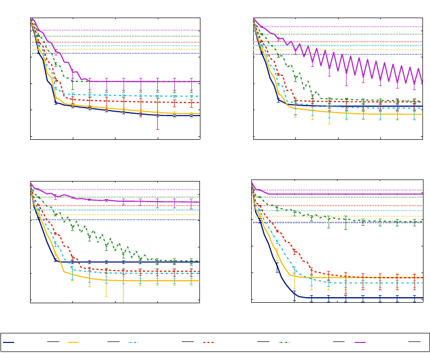
STATIC PREDICTION GAMES FOR ADVERSARIAL LEARNING PROBLEMS
0 10 20 30 40
10
-8
10
-6
10
-4
10
-2
10
0
ρ
+1
= 2
6
iterations
distance to NE
0 10 20 30 40
10
-8
10
-6
10
-4
10
-2
10
0
ρ
+1
= 2
4
iterations
distance to NE
0 10 20 30 40
10
-8
10
-6
10
-4
10
-2
10
0
ρ
+1
= 2
2
iterations
distance to NE
0 10 20 30 40
10
-8
10
-6
10
-4
10
-2
10
0
ρ
+1
= 1
iterations
distance to NE
ρ
−1
= 2
1
ρ
+1
ρ
−1
=
1
ρ
+1
ρ
−1
= 2
−1
1
ρ
+1
ρ
−1
= 2
−2
1
ρ
+1
ρ
−1
= 2
−4
1
ρ
+1
ρ
−1
= 2
−6
1
ρ
+1
Figure 1: Average Euclidean distance between the EDS solution and the ILS solution at iteration
k = 0,...,40 for Nash logistic regression on the ESP corpus. The dotted lines show the
distance between the EDS solution and the solution of logistic regression. Error bars
indicate standard deviation.
distinct equilibria. In the latter case, learner and data generator may attain distinct equilibria and
may experience an arbitrarily poor outcome when playing a Nash equilibrium.
6.2 Regularization Parameters
The regularization parameters ρ
v
of the players v ∈ {−1, +1} play a major role in the prediction
game. The learner’s regularizer determines the generalization ability of the predictive model and
the data generator’s regularizer controls the amount of change in the data generation process. In
order to tune these parameter, one would need to have access to labeled data that are governed by
the transformed input distribution. In our second experiment, we will explore to which extent those
parameters can be estimated using a portion of the newest training data. Intuitively, the most recent
training data may be more similar to the test data than older training data.
2645
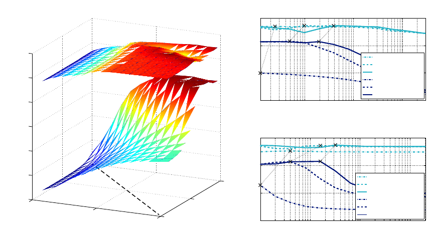
BR
¨
UCKNER, KANZOW, AND SCHEFFER
10
-4
10
-2
10
0
10
0
10
2
10
4
0.70
0.75
0.80
0.85
0.90
0.95
1.00
ρ
+1
Performance
ρ
−1
F-measure
hold-out data
test data
hold-out data
test data
10
-3
10
-2
10
-1
0.7
0.8
0.9
1.0
Fixed ρ
+1
ρ
−1
F-measure
ho (ρ
+1
= 1024)
ho (ρ
+1
= 8)
ho (ρ
+1
= 4)
te (ρ
+1
= 1024)
te (ρ
+1
= 8)
te (ρ
+1
= 4)
10
0
10
1
10
2
10
3
0.7
0.8
0.9
1.0
Fixed ρ
−1
ρ
+1
F-measure
ho (ρ
−1
= 0.125)
ho (ρ
−1
= 0.002)
ho (ρ
−1
= 0.0001)
te (ρ
−1
= 0.125)
te (ρ
−1
= 0.002)
te (ρ
−1
= 0.0001)
Figure 2: Left: Performance of NLR on the hold-out and the test data with respect to regularization
parameters. Right: Performance of NLR on the hold-out data (ho) and the test data (te)
for fixed values of ρ
v
.
We split the data set into three parts: The 2,000 oldest emails constitute the training portion, we
use the next 2,000 emails as hold-out portion on which the parameters are tuned, and the remaining
emails are used as test set. We randomly draw 200 spam and 200 non-spam messages from the train-
ing portion and draw another subset of 400 emails from the hold-out portion. Both NPG instances
are trained on the 400 training emails and evaluated against all emails of the test portion. To tune
the parameters, we conduct a grid search maximizing the likelihood on the 400 hold-out emails.
We repeat this experiment 10 times for all four data sets and report on the resulting parameters as
well as the “optimal” reference parameters according to the maximal value of F-measure on the test
set. Those optimal regularization parameters are not used in later experiments. The intuition of the
experiment is that the data generation process has already been changed between the oldest and the
latest emails. This change may cause a distribution shift which is reflected in the hold-out portion.
We expect that one can tune each players’ regularization parameter by tuning with respect to this
hold-out set.
In Figure 2 (left) we plot the performance of the Nash logistic regression (NLR) on the hold-out
and the test data against the regularization parameters ρ
−1
and ρ
+1
. The dashed line visualizes the
bound in (30) on the regularization parameters for which NLR is guaranteed to possess a unique
Nash equilibrium. Figure 2 (right) shows sectional views of the left plot along the ρ
−1
-axis (upper
diagram) and the ρ
+1
-axis (lower diagram) for several values of ρ
+1
and ρ
−1
, respectively. As
expected, the effect of the regularization parameters on the test data is much stronger than on the
hold-out data.
2646

STATIC PREDICTION GAMES FOR ADVERSARIAL LEARNING PROBLEMS
It turns out that the data generator’s ρ
+1
has almost no impact on the value of F-measure on
the hold-out data set (see lower right diagram of Figure 2). Hence, we conclude that estimating
ρ
+1
without access to labeled data from the test distribution or additional knowledge about the
data generator is difficult for this application; the most recent training data are still too different
from the test data. In all remaining experiments and for all data sets we set ρ
+1
= 8 for NLR and
ρ
+1
= 2 for NSVM. For those choices the Nash models performed generally best on the hold-out
set for a large variety of values of ρ
−1
. For Invar-SVM the regularization of the data generator’s
transformation is controlled explicitly by the number K of modifiable attributes per positive instance.
We conducted the same experiment for Invar-SVM resulting in an optimal value of K = 25; that is,
the data generator is allowed to remove up to 25 tokens of each spam email of the training data set.
From the upper right diagram of Figure 2 we see that estimating ρ
−1
for any fixed ρ
+1
seems
possible. Even if we slightly overestimate the learner’s optimal regularization parameter—to com-
pensate for the distributional difference between the transformed training sample and the marginal
shifted hold-out set—the determined value of ρ
−1
is close to the optimum for all four data sets.
6.3 Evaluation for Adversary Following an Equilibrium Strategy
We evaluate both a regular classifier trained under the i.i.d. assumption and a model that follows a
Nash equilibrium strategy against both an adversary who does not transform the input distribution
and an adversary who executes the Nash-equilibrial transformation on the input distribution. Since
we cannot be certain that actual s pam senders play a Nash equilibrium, we use the following semi-
artificial setting.
The learner observes a sample of 200 spam and 200 non-spam emails drawn from the training
portion of the data and estimates the Nash-optimal prediction model with parameters
˙
w; the trivial
baseline solution of regularized empirical risk minimization (ERM) is denoted by w. T he data
generator observes a distinct sample D of 200 spam and 200 non-spam messages, also drawn from
the training portion, and computes their Nash-optimal response
˙
D.
We again set c
v,i
:=
1
n
for v ∈ {−1,+1} and i = 1, . . .,n and study the following four scenarios:
• (w, D) : Both players ignore the presence of an opponent; that is, the learner employs a regular
classifier and the sender does not change the data generation process.
• (w,
˙
D) : The learner ignores the presence of an active data generator who changes the data
generation process such that D evolves to
˙
D by playing a Nash strategy.
• (
˙
w,D) : The learner expects a rational data generator and chooses a Nash-equilibrial predic-
tion model. However, the data generator does not change the input distribution.
• (
˙
w,
˙
D) : Both players are aware of the opponent and play a Nash-equilibrial action to secure
lowest costs.
We repeat this experiment 100 times for all four data sets. Table 2 reports on the average values
of F-measure over all repetitions and both NPG instances and corresponding baselines; numbers in
boldface indicate significant differences (α = 0.05) between the F-measures of f
w
and f
˙
w
for fixed
sample D and
˙
D, respectively.
As expected, when the data generator does not alter the input distribution, the regularized em-
pirical risk minimization baselines, logistic regression and the SVM, are generally best. However,
2647

BR
¨
UCKNER, KANZOW, AND SCHEFFER
NLR
vs.
LR
ESP
w
˙
w
D 0.957 0.924
˙
D
0.912 0.925
Mailinglist
w
˙
w
D 0.987 0.984
˙
D
0.958 0.976
Private
w
˙
w
D 0.961 0.944
˙
D
0.903 0.912
TREC 2007
w
˙
w
D 0.980 0.979
˙
D
0.955 0.961
NSVM
vs.
SVM
ESP
w
˙
w
D 0.955 0.939
˙
D
0.928 0.939
Mailinglist
w
˙
w
D 0.987 0.985
˙
D
0.961 0.976
Private
w
˙
w
D 0.961 0.957
˙
D
0.932 0.936
TREC 2007
w
˙
w
D 0.979 0.981
˙
D
0.960 0.968
Table 2: Nash predictor and regular classifier against passive and Nash-equilibrial data generator.
the performance of those baselines drops substantially when the data generator plays the Nash-
equilibrial action
˙
D. The Nash-optimal prediction models are more robust against this transforma-
tion of the input distribution and significantly outperform the reference methods for all four data
sets.
6.4 Case Study on Email Spam Filtering
To study the performance of the Nash prediction models and the baselines for email spam filtering,
we evaluate all methods into the future by processing the test set in chronological order. The test
portion of each data set is split into 20 chronologically sorted disjoint subsets. We average the value
of F-measure on each of those subsets over the 20 models (trained on different samples drawn from
the training portion) for each method and perform a paired t-test. In the absence of information
about player and instance-specific costs, we again set c
v,i
:=
1
n
for v ∈ {−1,+1}, i = 1,...,n. Note,
that the chosen loss functions and regularizers would allow us to select any positive cost factors
without violating Assumption 1.
Figure 3 shows that, for all data sets, the NPG instances outperform logistic regression (LR),
SVM, and SVMT that do not explicitly factor the adversary into the optimization criterion. Espe-
cially for the ESP corpus, the Nash logistic regression (NLR) and the Nash support vector machine
(NSVM) are superior. On the TREC 2007 data set, the methods behave comparably with a slight
advantage for the Nash support vector machine. The period over which the TREC 2007 data have
been collected is very short; we believe that the training and test instances are governed by nearly
identical distributions. Consequently, for this data set, the game theoretic models do not gain a
significant advantage over logistic regression and the SVM that assume i.i.d. samples. With respect
to the non-game theoretic baselines, the regular SVM outperforms LR and SVMT for most of the
data sets.
Table 3 shows aggregated results over all four data sets. For each point in each of the diagrams of
Figure 3, we conduct a pairwise comparison of all methods based on a paired t-test at a confidence
level of α = 0.05. When a difference is significant, we count this as a win for the method that
achieves a higher value of F-measure. Each line of Table 3 details the wins and, set in italics, the
losses of one method against all other methods.
The Nash logistic regression and the Nash support vector machine have more wins than they
have losses against each of the other methods. The ranking continues with Invar-SVM, the regular
SVM, logistic regression and the trigonometric loss SVM which loses more frequently than it wins
against all other methods.
2648
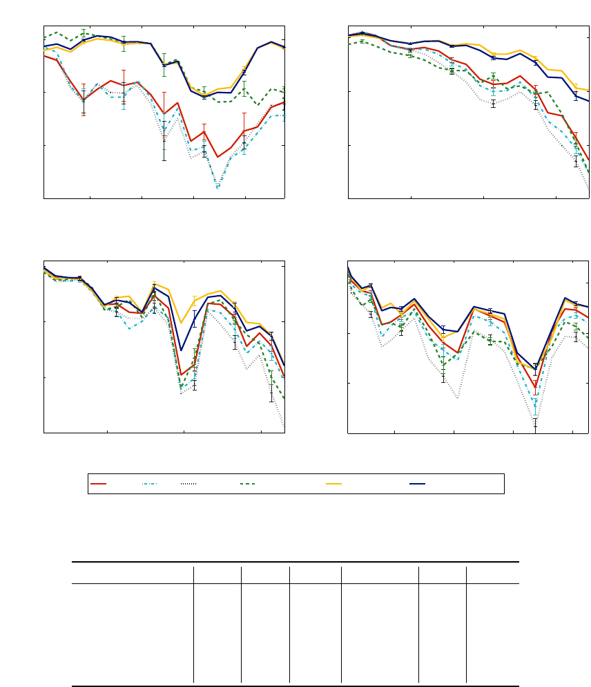
STATIC PREDICTION GAMES FOR ADVERSARIAL LEARNING PROBLEMS
Dec07 Jul08 Jan09 Aug09
0.76
0.82
0.88
0.94
F-measure
Performance on ESP corpus
Oct02 Feb04 Jul05
0.87
0.91
0.95
0.99
Performance on Mailinglist corpus
F-measure
Nov06 Apr08 Aug09
0.64
0.75
0.86
0.97
Performance on Private corpus
F-measure
Apr07 May07 Jun07 Jun07
0.93
0.95
0.97
0.99
Performance on TREC 2007 corpus
F-measure
SVM LR TSVM Invar-SVM NLR (ILS) NSVM (ILS)
Figure 3: Value of F-measure of predictive models. Error bars indicate standard errors.
method vs. method SVM LR SVMT Invar-SVM NLR NSVM
SVM 0:0 40:2 53:0 30:20 8:57 2:65
LR
2:40 0:0 49:5 19:29 5:59 2:71
SVMT 0:53 5:49 0:0 9:47 2:70 2:74
Invar-SVM
20:30 29:19 47:9 0:0 5:57 3:57
NLR 57:8 59:5 70:2 57:5 0:0 22:30
NSVM 65:2 71:2 74:2 57:3 30:22 0:0
Table 3: Results of paired t-test over all corpora: Number of trials in which each method (row)
has significantly outperformed each other method (column) vs. number of times it was
outperformed.
6.5 Efficiency versus Effectiveness
To assess the predictive performance as well as the execution time as a function of the sample size,
we train the baselines and the two NPG instances for a varying number of training examples. We
2649
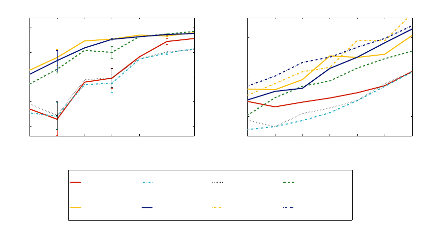
BR
¨
UCKNER, KANZOW, AND SCHEFFER
50 100 200 400 800 1600 3200
0.75
0.8
0.85
0.9
0.95
Performance on ESP corpus
number of training emails
F-measure
50 100 200 400 800 1600 3200
10
-1
10
1
10
3
Execution time on ESP corpus
number of training emails
time in sec
SVM LR TSVM Invar-SVM
NLR (ILS) NSVM (ILS) NLR (EDS) NSVM (EDS)
Figure 4: Predictive performance (left) and execution time (right) for varying sizes of the training
data set.
report on the results for the ESP data set in Figure 4. The game theoretic models significantly
outperform the trivial baseline methods logistic regression, the SVM and the SVMT, especially for
small data sets. However, this comes at the price of considerably higher computational cost. The
ILS algorithm requires in general only a couple of iterations to converge; however in each iteration
several optimization problems have to be solved so that the total execution time is up to a factor
150 larger than that of the corresponding ERM baseline. In contrast to the ILS algorithm, a single
iteration of the EDS algorithm does not require solving nested optimization problems. However, the
execution time of the EDS algorithm is still higher as it often requires several thousand iterations
to fully converge. For larger data sets, the discrepancy in predictive performance between game
theoretic models and i.i.d. baseline decreases. Our results do not provide conclusive evidence
whether ILS or EDS is faster at solving the optimization problems. We conclude that the benefit of
the NPG prediction models over the classification baseline is greatest for small to medium sample
sizes.
6.6 Nash-Equilibrial Transformation
In contrast to Invar-SVM, the Nash models allow the data generator to modify non-spam emails.
However in pr actice most senders of legitimate messages do not deliberately change their writing
behavior in order to bypass spam filters, perhaps with the exception of senders of newsletters who
must be careful not to trigger filtering mechanisms.
In a final experiment, we want to study whether the Nash model reflects this aspect of reality,
and how the data generator’s regularizer effects this transformation. The training portion contains
again n
+1
= 200 spam and n
−1
= 200 non-spam instances randomly chosen from the oldest 4,000
2650

STATIC PREDICTION GAMES FOR ADVERSARIAL LEARNING PROBLEMS
emails. We determine the Nash equilibrium and measure the number of additions and deletions to
spam and non-spam emails in
˙
D:
∆
add
−1
:=
1
n
−1
∑
i:y
i
=−1
m
∑
j=1
max(0,
˙
x
i, j
−x
i, j
)
∆
add
+1
:=
1
n
+1
∑
i:y
i
=+1
m
∑
j=1
max(0,
˙
x
i, j
−x
i, j
)
∆
del
−1
:=
1
n
−1
∑
i:y
i
=−1
m
∑
j=1
max(0,x
i, j
−
˙
x
i, j
)
∆
del
+1
:=
1
n
+1
∑
i:y
i
=+1
m
∑
j=1
max(0,x
i, j
−
˙
x
i, j
)
where x
i, j
indicates the presence of token j in the i-th tr aining email, that is, ∆
add
v
and ∆
del
v
denote
the average number of word additions and deletions per spam and non-spam email performed by
the sender.
Figure 5 shows the number of additions and deletions of the Nash transformation as a function
of the adversary’s regularization parameter for the ESP data set. Table 4 reports on the average
number of word additions and deletions for all data sets. For Invar-SVM, we set the number of
possible deletions to K = 25.
ESP
game non-spam spam
model add del add del
Invar-SVM 0.0 0.0 0.0 24.8
NLR 0.7 1.0 22.5 31.2
NSVM 0.4 0.5 17.9 23.8
Mailinglist
game non-spam spam
model add del add del
Invar-SVM 0.0 0.0 0.0 23.9
NLR
0.3 0.4 8.6 10.9
NSVM 0.3 0.3 6.9 8.4
Private
game non-spam spam
model add del add del
Invar-SVM 0.0 0.0 0.0 24.2
NLR
0.4 0.2 24.3 11.2
NSVM 0.1 0.1 15.6 7.3
TREC 2007
game non-spam spam
model add del add del
Invar-SVM 0.0 0.0 0.0 24.7
NLR
0.2 0.2 15.0 11.4
NSVM 0.2 0.1 11.1 8.4
Table 4: Average number of word additions and deletions per training email.
The Nash-equilibrial transformation imposes almost no changes on any non-spam email; the
number of modifications declines as the regularization parameter grows (see Figure 5). We observe
for all data s ets that even if the total amount of transformation differs for NLR and NSVM, both
instances behave similarly insofar as the number of word additions and deletions continues to grow
when the adversary’s regularizer decreases.
7. Conclusion
We studied prediction games in which the learner and the data generator have conflicting but not
necessarily directly antagonistic cost functions. We focused on static games in which learner and
data generator have to commit simultaneously to a predictive model and a transformation of the
input distribution, r espectively.
The cost-minimizing action of each player depends on the opponent’s move; in the absence
of information about the opponent’s move, players may choose to play a Nash equilibrium strategy
2651
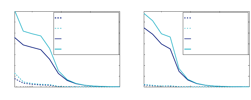
BR
¨
UCKNER, KANZOW, AND SCHEFFER
10
0
10
1
10
2
0
10
20
30
40
50
60
70
Amount of transformation for NLR
ρ
+1
number of modifications
non-spam additions ∆
add
-1
non-spam deletions ∆
del
-1
spam additions ∆
add
+1
spam deletions ∆
del
+1
10
0
10
1
10
2
0
5
10
15
20
25
30
35
Amount of transformation for NSVM
ρ
+1
number of modifications
non-spam additions ∆
add
-1
non-spam deletions ∆
del
-1
spam additions ∆
add
+1
spam deletions ∆
del
+1
Figure 5: Average number of additions and deletions per spam/non-spam email for NLR (left)
and NSVM (right) with respect to the adversary’s regularization parameter ρ
+1
for fixed
ρ
−1
= n
−1
.
which constitutes a cost-minimizing move for each player if the other player follows the equilibrium
as well. Because a combination of actions from distinct equilibria may lead to arbitrarily high costs
for either player, we have studied conditions under which a prediction game can be guaranteed
to possess a unique Nash equilibrium. Lemma 1 identifies conditions under which at least one
equilibrium exists, and Theorem 8 elaborates on when this equilibrium is unique. We propose
an inexact linesearch approach and a modified extragradient approach for identifying this unique
equilibrium. Empirically, both approaches perform quite similarly.
We derived Nash logistic regression and Nash support vector machine models and kernelized
versions of these methods. Corollaries 11 and 15 specialize Theorem 8 and expound conditions
on the player’s regularization parameters under which the Nash logistic regression and the support
vector machine converge on a unique Nash equilibrium. Empirically, we find that both methods
identify unique Nash equilibria when the bounds laid out in Corollaries 11 and 15 are satisfied or
violated by a factor of up to 4. From our experiment on several email corpora we conclude that Nash
logistic regression and the support vector machine outperform their i.i.d. baselines and Invar-SVM
for the problem of classifying future emails based on training data from the past.
Acknowledgments
This work was supported by the German Science Foundation (DFG) under grant
SCHE540/12-1 and by STRATO AG. We thank Niels Landwehr and Christoph Sawade for con-
structive comments and suggestions, and the anonymous reviewer for helpful contributions and
careful proofreading of the manuscript!
2652
STATIC PREDICTION GAMES FOR ADVERSARIAL LEARNING PROBLEMS
References
Tamer Basar and Geert J. Olsder. Dynamic Noncooperative Game Theory. Society for Industrial
and Applied Mathematics, 1999.
Stephen Boyd and Lieven Vandenberghe. Convex Optimization. Cambridge University Press, 2004.
Michael Br
¨
uckner and Tobias Scheff er. Nash equilibria of static prediction games. In Advances in
Neural Information Processing Systems. MIT Press, 2009.
Michael Br
¨
uckner and Tobias Scheffer. Stackelberg games for adversarial prediction problems. In
Proceedings of the 17th ACM SIGKDD International Conference on Knowledge Discovery and
Data Mining (KDD), San Diego, CA, USA. ACM, 2011.
Ofer Dekel and Ohad Shamir. Learning to classify with missing and corrupted features. In Pro-
ceedings of the International Conference on Machine Learning. ACM, 2008.
Ofer Dekel, Ohad Shamir, and Lin Xiao. Learning to classify with missing and corr upted features.
Machine Learning, 81(2):149–178, 2010.
Carl Geiger and Christian Kanzow. Theorie und Numerik restringierter Optimierungsaufgaben.
Springer, 1999.
Laurent El Ghaoui, Gert R. G. Lanckriet, and Georges Natsoulis. Robust classification with in-
terval data. Technical Report UCB/CSD-03-1279, EECS Department, University of California,
Berkeley, 2003.
Amir Globerson and Sam T. Roweis. Nightmare at test time: Robust learning by feature deletion.
In Proceedings of the International Conference on Machine Learning. ACM, 2006.
Amir Globerson, Choon Hui Teo, Alex J. Smola, and Sam T. Roweis. An adversarial view of
covariate shift and a minimax approach. In Dataset Shift in Machine Learning, pages 179–198.
MIT Press, 2009.
Patrick T. Harker and Jong-Shi Pang. Finite-dimensional variational inequality and nonlinear com-
plementarity problems: A s urvey of theory, algorithms and applications. Mathematical Program-
ming, 48(2):161–220, 1990.
Roger A. Horn and Charles R. Johnson. Topics in Matrix Analysis. Cambridge University Press,
Cambridge, 1991.
James T. Kwok and Ivor W. Tsang. The pre-image problem in kernel methods. In Proceedings
of International Conference on Machine Learning, pages 408–415. AAAI Press, 2003. ISBN
1-57735-189-4.
Gert R. G. Lanckriet, Laurent El Ghaoui, Chiranjib Bhattacharyya, and Michael I. Jordan. A robust
minimax approach to classification. Journal of Machine Learning Research, 3:555–582, 2002.
Sebastian Mika, Bernhard Sch
¨
olkopf, Alex J. Smola, Klaus-Robert M
¨
uller, Matthias Scholz, and
Gunnar R
¨
atsch. Kernel PCA and de–noising in feature spaces. In Advances in Neural Information
Processing Systems. MIT Press, 1999.
2653
BR
¨
UCKNER, KANZOW, AND SCHEFFER
J. Ben Rosen. Existence and uniqueness of equilibrium points for concave n-person games. Econo-
metrica, 33(3):520–534, 1965.
Bernhard Sch
¨
olkopf and Alex J. Smola. Learning with Kernels. The MIT Press, Cambridge, MA,
2002.
Bernhard Sch
¨
olkopf, Ralf Herbrich, and Alex J. Smola. A generalized representer theorem. In
COLT: Proceedings of the Workshop on Computational Learning Theory, Morgan Kaufmann
Publishers, 2001.
Christian Siefkes, Fidelis Assis, Shalendra Chhabra, and William S. Yerazunis. Combining Winnow
and orthogonal sparse bigrams for incremental spam filtering. In Proceedings of the 8th European
Conference on Principles and Practice of Knowledge Discovery in Databases (PKDD), volume
3202 of Lecture Notes in Artificial Intelligence, pages 410–421. Springer, 2004.
Choon Hui Teo, Amir Globerson, Sam T. Roweis, and Alex J. Smola. Convex learning with invari-
ances. In Advances in Neural Information Processing Systems. MIT Press, 2007.
Anna von Heusinger and Christian Kanzow. Relaxation methods for generalized Nash equilibrium
problems with inexact line search. Journal of Optimization Theory and Applications, 143(1):
159–183, 2009.
2654
