Microsoft PowerPoint - Berk_DeMarzo_cf5_ppt

Corporate Finance

Fifth Edition

Chapter 9

Valuing Stocks

Chapter Outline

9.1 The Dividend-Discount Model

9.2 Applying the Dividend-Discount Model

9.3 Total Payout and Free Cash Flow Valuation Models

9.4 Valuation Based on Comparable Firms

9.5 Information, Competition, and Stock Prices

Siemens AG Dividends

SIEMENS AG Dividend Payment

Type Div. Rate Tax XD Date Pay Date

YR E 3.80 +3 % (G) 31.01.2019 04.02.2019

YR E 3.70 +3 % (G) 01.02.2018 05.02.2018

YR E 3.60 +3 % (G) 02.02.2017 06.02.2017

YR E 3.50 +6 % (G) 27.01.2016 27.01.2016

YR E 3.30 +10% (G) 28.01.2015 28.01.2015

YR E 3.00 +0 % (G) 29.01.2014 29.01.2014

YR E 3.00 +0 % (G) 24.01.2013 24.01.2013

YR E 3.00 +11% (G) 25.01.2012 25.01.2012

YR E 2.70 +69% (G) 26.01.2011 26.01.2011

YR E 1.60 +0 % (G) 27.01.2010 27.01.2010

YR E 1.60 +0 % (G) 28.01.2009 28.01.2009

YR E 1.60 +10% (G) 25.01.2008 25.01.2008

YR E 1.45 +7% (G) 26.01.2007 26.01.2007

YR E 1.35 +8% (G) 27.01.2006 27.01.2006

YR E 1.25 +14% (G) 28.01.2005 28.01.2005

YR E 1.10 +10% (G) 23.01.2004 23.01.2004

YR E 1.00 (G) 24.01.2003 24.01.2003

YR E 1.00 (G) 18.01.2002 18.01.2002

SPL E 1.00 (G) 23.02.2001 23.02.2001

YR E 1.40 (G) 23.02.2001 23.02.2001

YR E 1.00 (G) 25.02.2000 25.02.2000

YR DM1.50 (G) 19.02.1999 19.02.1999

YR DM1.50 (G) 20.02.1998 20.02.1998

YR DM1.50 (G) 14.02.1997 14.02.1997

YR DM13.00 (G) 23.02.1996 23.02.1996

YR DM13.00 (G) 24.02.1995 24.02.1995

Mc Donalds Dividends

Type Div. Rate Tax XD Date Pay Date

QTR U$1.16 +15% (G) 30.11.2018 17.12.2018

QTR U$1.01 (G) 31.08.2018 18.09.2018

QTR U$1.01 (G) 01.06.2018 18.06.2018

QTR U$1.01 (G) 28.02.2018 15.03.2018

QTR U$1.01 +7 % (G) 30.11.2017 15.12.2017

QTR U$0.94 (G) 30.08.2017 18.09.2017

QTR U$0.94 (G) 01.06.2017 19.06.2017

QTR U$0.94 (G) 27.02.2017 15.03.2017

QTR U$0.94 +6 % (G) 29.11.2016 15.12.2016

QTR U$0.89 (G) 30.08.2016 16.09.2016

QTR U$0.89 (G) 02.06.2016 20.06.2016

QTR U$0.89 (G) 26.02.2016 15.03.2016

QTR U$0.89 +5 % (G) 27.11.2015 15.12.2015

QTR U$0.85 (G) 28.08.2015 16.09.2015

QTR U$0.85 (G) 28.05.2015 15.06.2015

QTR U$0.85 (G) 26.02.2015 16.03.2015

QTR U$0.85 +5 % (G) 26.11.2014 15.12.2014

QTR U$0.81 (G) 28.08.2014 16.09.2014

QTR U$0.81 (G) 29.05.2014 16.06.2014

QTR U$0.81 (G) 27.02.2014 17.03.2014

QTR U$0.81 +5 % (G) 27.11.2013 16.12.2013

QTR U$0.77 (G) 29.08.2013 17.09.2013

QTR U$0.77 (G) 30.05.2013 17.06.2013

QTR U$0.77 (G) 27.02.2013 15.03.2013

QTR U$0.77 +10 % (G) 29.11.2012 17.12.2012

QTR U$0.70 (G) 30.08.2012 18.09.2012

QTR U$0.70 (G) 31.05.2012 15.06.2012

QTR U$0.70 (G) 28.02.2012 15.03.2012

QTR U$0.70 +15 % (G) 29.11.2011 15.12.2011

Type Div. Rate Tax XD Date Pay Date

QTR U$1.25 +8% (G) 29.11.2019 16.12.2019

QTR U$1.16 (G) 30.08.2019 17.09.2019

QTR U$1.16 (G) 31.05.2019 17.06.2019

QTR U$1.16 (G) 28.02.2019 15.03.2019

QTR U$1.16 (G) 30.11.2018 17.12.2018

Learning Objectives (1 of 4)

• Describe, in words, the Law of One Price value for a

common stock, including the discount rate that should be

used.

• Calculate the total return of a stock, given the dividend

payment, the current price, and the previous price.

• Use the dividend-discount model to compute the value of a

dividend-paying company’s stock, whether the dividends

grow at a constant rate starting now or at some time in the

future.

Mc Donalds Dividends

Type Div. Rate Tax XD Date Pay Date

QTR U$0.61 (G) 30.08.2011 16.09.2011

QTR U$0.61 (G) 27.05.2011 15.06.2011

QTR U$0.61 (G) 25.02.2011 15.03.2011

QTR U$0.61 +11 % (G) 29.11.2010 15.12.2010

QTR U$0.55 (G) 30.08.2010 16.09.2010

QTR U$0.55 (G) 27.05.2010 15.06.2010

QTR U$0.55 (G) 25.02.2010 15.03.2010

QTR U$0.55 +10 % (G) 27.11.2009 15.12.2009

QTR U$0.50 (G) 28.08.2009 15.09.2009

QTR U$0.50 (G) 04.06.2009 22.06.2009

QTR U$0.50 (G) 26.02.2009 16.03.2009

QTR U$0.50 (G) 26.11.2008 15.12.2008

QTR U$0.375 (G) 28.08.2008 16.09.2008

QTR U$0.375 (G) 05.06.2008 23.06.2008

QTR U$0.375 (G) 28.02.2008 17.03.2008

YR U$1.50 (G) 13.11.2007 03.12.2007

YR U$1.00 (G) 13.11.2006 01.12.2006

YR U$0.67 (G) 10.11.2005 01.12.2005

YR U$0.55 (G) 10.11.2004 01.12.2004

YR U$0.40 (G) 12.11.2003 01.12.2003

YR U$0.235 (G) 13.11.2002 02.12.2002

YR U$0.225 (G) 13.11.2001 03.12.2001

YR U$0.215 (G) 13.11.2000 01.12.2000

QTR U$0.04875 (G) 29.11.1999 15.12.1999

QTR U$0.04875 (G) 30.08.1999 15.09.1999

QTR U$0.04875 (G) 27.05.1999 15.06.1999

QTR U$0.0488 (G) 11.03.1999 31.03.1999

QTR U$0.09 (G) 25.11.1998 11.12.1998

QTR U$0.09 (G)

Learning Objectives (2 of 4)

• Discuss the determinants of future dividends and growth

rate in dividends, and the sensitivity of the stock price to

estimate those two factors.

• Given the retention rate and the return on new investment,

calculate the growth rate in dividends, earnings, and share

price.

• Describe circumstances in which cutting the firm’s dividend

will raise the stock price.

Learning Objectives (3 of 4)

• Assuming a firm has a long-term constant growth rate after

time N + 1, use the constant growth model to calculate the

terminal value of the stock at time N.

• Compute the stock value of a firm that pays dividends as

well as repurchasing shares.

• Use the discounted free cash flow model to calculate the

value of stock in a company with leverage.

• Use comparable firm multiples to estimate stock value.

• Explain why several valuation models are required to value

a stock.

Learning Objectives (4 of 4)

• Describe the impact of efficient markets hypothesis on

positive-N P V trades by individuals with no inside

information.

• Discuss why investors who identify positive-N P V trades

should be skeptical about their findings, unless they have

inside information or a competitive advantage. As part of

that, describe the return the average investor should

expect to get.

• Assess the impact of stock valuation on recommended

managerial actions.

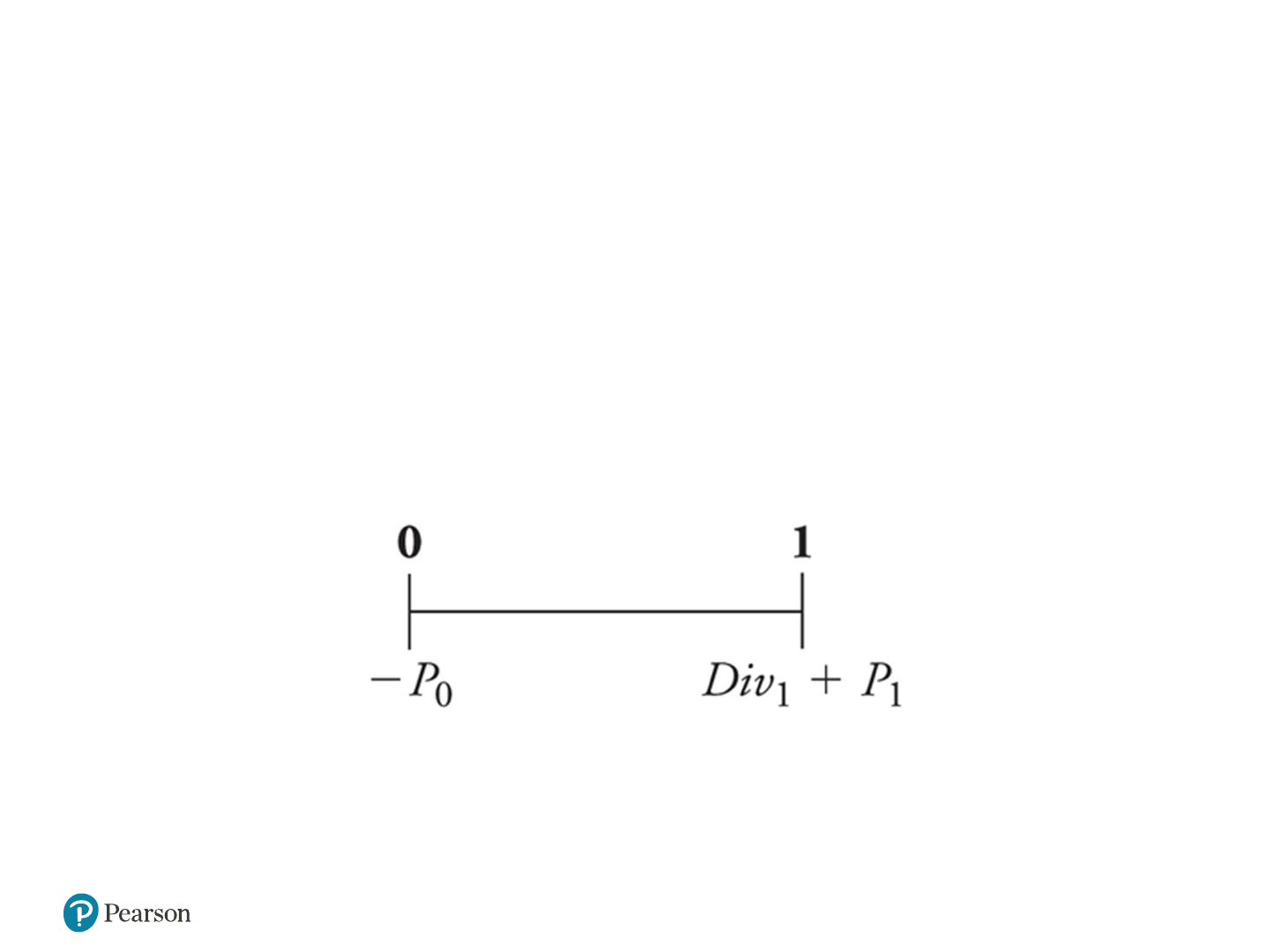
9.1 The Dividend-Discount Model (1 of 2)

• A One-Year Investor

– Potential Cash Flows

 Dividend

 Sale of Stock

– Timeline for One-Year Investor

• Since the cash flows are risky, we must discount them at

the equity cost of capital

9.1 The Dividend-Discount Model (2 of 2)

• A One-Year Investor

11

0

+

=

1 +

E

D

iv P

P

r







– If the current stock price were less than this amount,

expect investors to rush in and buy it, driving up the

stock’s price

– If the stock price exceeded this amount, selling it would

cause the stock price to quickly fall

Dividend Yields, Capital Gains, and

Total Returns



10

11 1

000

= 1

E

D

ividend Yield Capital Gain Rate

PP

Div P Div

r

PPP





 

• Dividend Yield

• Capital Gain

– Capital Gain Rate

• Total Return

– Dividend Yield + Capital Gain Rate

 The expected total return of the stock should equal the

expected return of other investments available in the market

with equivalent risk

Textbook Example 9.1 (1 of 2)

Stock Prices and Returns

Problem

Suppose you expect Walgreens Boots Alliance (a drugstore

chain) to pay dividends of $1.60 per share and trade for $70

per share at the end of the year. If investments with

equivalent risk to Walgreen’s stock have an expected return

of 8.5%, what is the most you would pay today for

Walgreen’s stock? What dividend yield and capital gain rate

would you expect at this price?

Textbook Example 9.1 (2 of 2)

Solution

Using Eq. 9.1, we have

11

0

1.60 70.00

= $65.99

1+ 1.085

E

Div p

P

r





At this price, Walgreen’s dividend yield is

1

0

1.60

2.42%.

65.99

Div

P



The expected capital gain is $70.00 − $65.99 = $4.01 per

share, for a capital gain rate of

4.01

6.08%.

65.99



Therefore, at this price, Walgreen’s expected total return is

2.42% + 6.08% = 8.5%, which is equal to its equity cost of

capital.

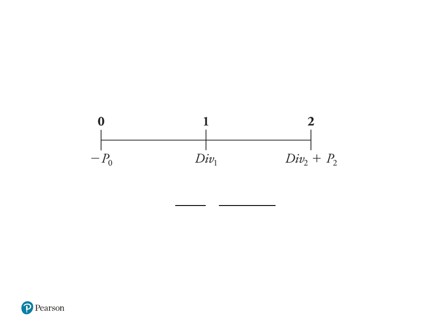
A Multi-Year Investor

• What is the price if we plan on holding the stock for two

years?

122

0

2

1 (1 )

EE

Div Div P

P

rr







The Dividend-Discount Model Equation

(1 of 2)

• What is the price if we plan on holding the stock for N

years?

12

0

2

1 (1 ) (1 ) (1 )

NN

EE E E

Div P

Div Div

P

rr r r

  

  

– This is known as the Dividend-Discount Model

 Note that the above equation (9.4) holds for any

horizon N

– Thus all investors (with the same beliefs) will

attach the same value to the stock, independent

of their investment horizons

The Dividend-Discount Model Equation

(2 of 2)

• The price of any stock is equal to the present value of the

expected future dividends it will pay

3

12

0

23

1

EE E E

1 (1 ) (1 ) (1 )





  

  





n

Div Div

P

rr r r

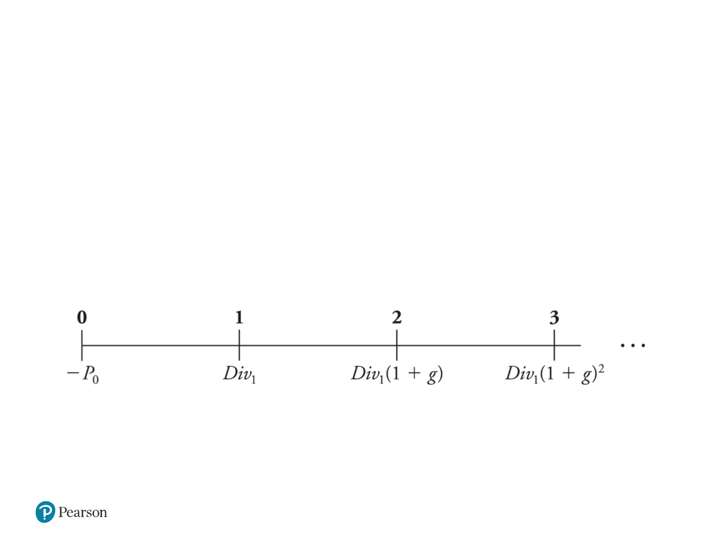
9.2 Applying the Discount-Dividend

Model

(1 of 2)

• Constant Dividend Growth

– The simplest forecast for the firm’s future dividends

states that they will grow at a constant rate, g, forever

9.2 Applying the Discount-Dividend

Model

(2 of 2)

• Constant Dividend Growth Model

1

0

=

E

Div

P

r

g



1

0

= +

E

Div

r

g

P

– The value of the firm depends on the current dividend

level, the cost of equity, and the growth rate

Textbook Example 9.2 (1 of 2)

Valuing a Firm with Constant Dividend Growth

Problem

Consolidated Edison, Inc. (Con Edison), is a regulated utility

company that services the New York City area. Suppose

Con Edison plans to pay $3.00 per share in dividends in the

coming year. If its equity cost of capital is 6% and dividends

are expected to grow by 2% per year in the future, estimate

the value of Con Edison’s stock.

Textbook Example 9.2 (2 of 2)

Solution

If dividends are excepted to grow perpetually at a rate of 2%

per year, we can use Eq. 9.6 to calculate the price of a share

of Con Edison stock:

1$3.00

== =$75

0.06 0.02

O

E

Div

P

rg

Dividends Versus Investment and

Growth

(1 of 6)

• A Simple Model of Growth

– Dividend Payout Ratio

 The fraction of earnings paid as dividends each year

t

t t

t

EPS

Earnings

= × Dividend Pa

y

out Rate

Shares Outstanding

Div



Earnings per Share

Dividends Versus Investment and

Growth

(2 of 6)

• A Simple Model of Growth

– Assuming the number of shares outstanding is

constant, the firm can do two things to increase its

dividend:

 Increase its earnings (net income)

 Increase its dividend payout rate

Dividends Versus Investment and

Growth

(3 of 6)

• A Simple Model of Growth

– A firm can do one of two things with its earnings:

 It can pay them out to investors

 It can retain and reinvest them

Dividends Versus Investment and

Growth

(4 of 6)

• A Simple Model of Growth

Change in Earnings = Earnings × Retention Rate × Return on New Investment

New Investment = Earnin

g

s × Retention Rate

– Retention Rate

 Fraction of current earnings that the firm retains

Notice: Dividend Payout Ratio = 1 – Retention Rate

Change in Earnings = New Investment × Return on New Investment

Dividends Versus Investment and

Growth

(5 of 6)

• A Simple Model of Growth

Change in Earnings

g = Earnings Growth Rate

Earnings

Earnings × Retention Rate × Return on New Investment

= Earnings Growth Rate

Earnings

Retention Rate × Return on New Investment



g = Retention Rate × Return on New Investment

– If the firm keeps its retention rate constant, then the

growth rate in dividends will equal the growth rate of

earnings

Change in Earnings = Earnings

× Retention Rate

× Return on New Investment

Dividends Versus Investment and

Growth

(6 of 6)

• Profitable Growth

– If a firm wants to increase its share price, should it cut

its dividend and invest more, or should it cut

investment and increase its dividend?

 The answer will depend on the profitability of the

firm’s investments

– Cutting the firm’s dividend to increase

investment will raise the stock price if, and only

if, the new investments have a positive NPV.

Textbook Example 9.3 (1 of 3)

Cutting Dividends for Profitable Growth

Problem

Crane sporting goods expect to have earnings per share of $6 in

the coming year. Rather than reinvest these earnings and grow,

the firm plans to pay out all of its earnings as a dividend. With

these expectations of no growth, Crane’s current share price is

$60.

Suppose crane could cut its dividend payout rate to 75% for the

foreseeable future and use the retained earnings to open new

stores. The return on its investment in these stores is expected to

be 12%. Assuming its equity cost of capital is unchanged, what

effect would this new policy have on Crane’s stock price?

Textbook Example 9.3 (2 of 3)

Solution

First, let’s estimate Crane’s equity cost of capital. Currently, Crane plans to pay

a dividend equal to its earnings of $6 per share. Given a share price of $60,

Crane’s dividend yield is With no expected growth (g = 0),

$6

=10%.

$60

we can use Eq. 9.7 to estimate r

E:

1

0

+10%+0%10%

E

Div

rg

P

 

In other words, to justify Crane’s stock price under its current policy, the expected

return of other stocks in the market with equivalent risk must be 10%.

Next, we consider the consequences of the new policy. If Crane reduces its

dividend payout rate to 75%, then from Eq. 9.8 its dividend this coming year will

fall to Div

1

= EPS1 × 75% = $6 × 75% = $4.50. At the same time, because the

firm will now retain 25% of its earnings to invest in new stores, from Eq. 9.12 its

growth rate will increase to

Textbook Example 9.3 (3 of 3)

g = Retention Rate × Return on New Investment = 25% × 12% =

3%

Assuming Crane can continue to grow at this rate, we can

compute its share price under the new policy using the constant

dividend growth model of Eq. 9.6:

1

0

$4.50

$64.29

0.10 0.03

E

Div

P

rg

 



Thus, Crane’s share price should rise from $60 to $64.29 if it cuts

its dividend to invest in projects that offer a return (12%) greater

than their cost of capital (which we assume remains 10%). These

projects are positive N P V , and so by taking them Crane has

created value for its shareholders.

Textbook Example 9.4 (1 of 2)

Unprofitable Growth

Problem

Suppose Crane Sporting Goods decides to cut its dividend

payout rate to 75% to invest in new stores, as in Example

9.3 but now suppose that the return on these new

investments is 8%, rather than 12%. Given its excepted

earnings per share this year of $6 and its equity cost of

capital of 10%, what will happen to Crane’s current share

price in this case?

Textbook Example 9.4 (2 of 2)

Solution

Just as in Example 9.3, Crane’s dividend will fall to $6 × 75%

= $4.50. Its growth rate under the new policy, given the lower

return on new investment, will now be g = 25% × 8% = 2%.

The new share price is there fore

1

0

$4.50

$56.25

0.10 0.02

E

Div

P

rg

 



Thus, even though Crane will grow under the new policy, the

new investments have negative NPV. Crane’s share price

will fall if it cuts its dividend to make new investments with a

return of only 8% when its investors can earn 10% on other

investments with comparable risk.

Changing Growth Rates (1 of 3)

• We cannot use the constant dividend growth model to

value a stock if the growth rate is not constant

– For example, young firms often have very high initial

earnings growth rates

– During this period of high growth, these firms often

retain 100% of their earnings to exploit profitable

investment opportunities

– As they mature, their growth slows

– At some point, their earnings exceed their investment

needs, and they begin to pay dividends

Changing Growth Rates (2 of 3)

• Although we cannot use the constant dividend growth

model directly when growth is not constant, we can use the

general form of the model to value a firm by applying the

constant growth model to calculate the future share price

of the stock once the expected growth rate stabilizes

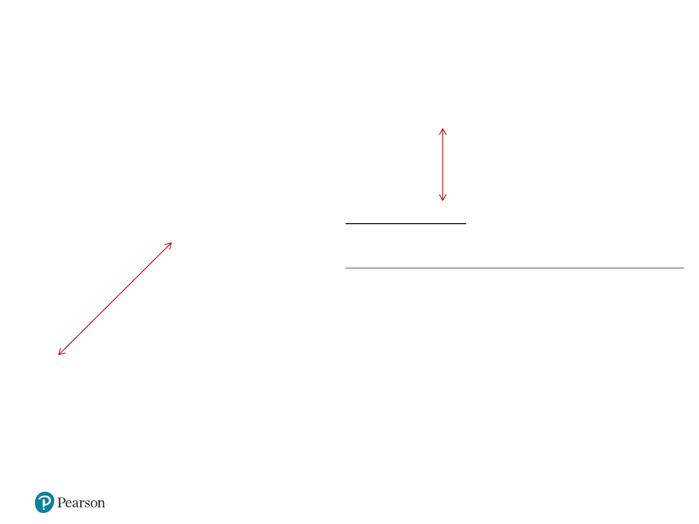
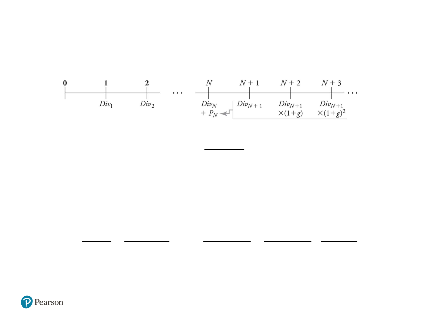
Changing Growth Rates (3 of 3)

+ 1

N

E

Div

P

r

g





• Dividend-Discount Model with Constant Long-Term Growth

1

12

0

2

1

1 + (1 + ) (1 + ) (1 + )

NN+

NN

EE E EE

Div Div

PL

rr r rrg



  







Textbook Example 9.5 (1 of 3)

Valuing a Firm with Two Different Growth Rates

• Problem

– Small Fry, Inc., has just invented a potato chip that looks

and tastes like a french fry. Given the phenomenal market

response to this product, Small Fry is reinvesting all of its

earnings to expand its operations. Earnings were $2 per

share this past year and are expected to grow at a rate of

20% per year until the end of year 4. At that point, other

companies are likely to bring out competing products.

Analysts project that at the end of year 4, Small Fry will cut

investment and begin paying 60% of its earnings as

dividends and its growth will slow to a long-run rate of 4%. If

Small Fry’s equity cost of capital is 8%, what is the value of

a share today?

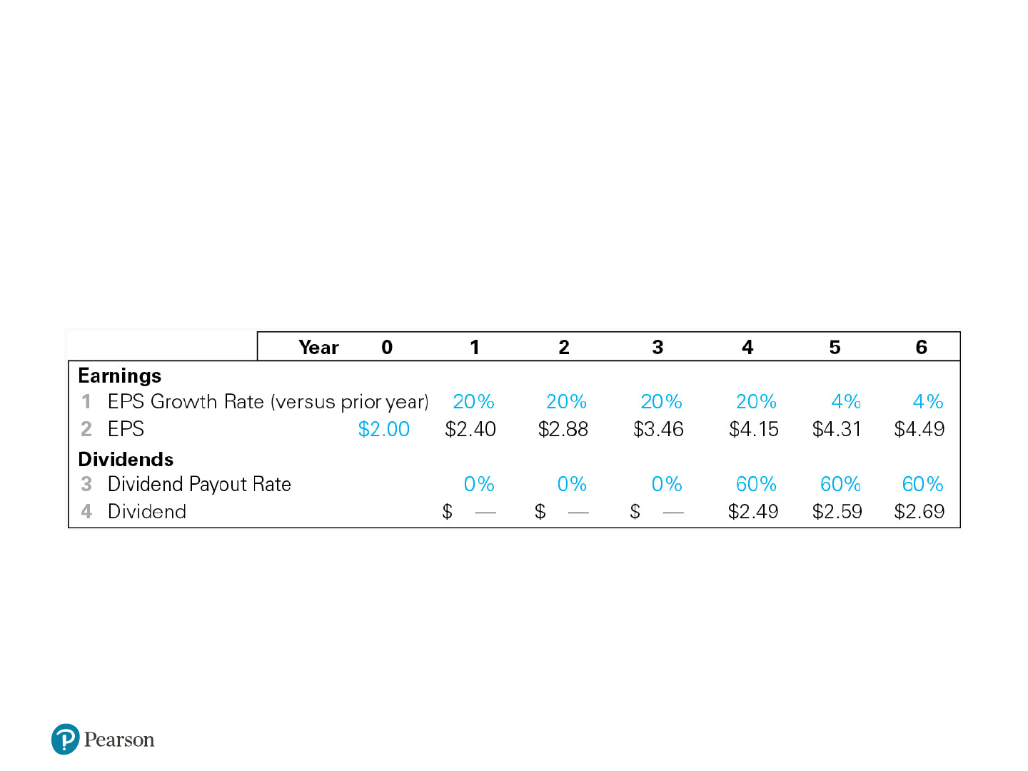
Textbook Example 9.5 (2 of 3)

Solution

We can use Small Fry’s projected earnings growth rate and payout rate

to forecast its future earnings and dividends as shown in the following

spreadsheet:

Starting from $2.00 in year 0, E P S grows by 20% per year until year 4,

after which growth slows to 4%. Small Fry’s dividend payout rate is zero

until year 4, when competition reduces its investment opportunities and

its payout rate rises to 60%. Multiplying E P S by the dividend payout ratio,

we project Small Fry’s future dividends in line 4.

Textbook Example 9.5 (3 of 3)

From year 4 onward, Small Fry’s dividends will grow at the

expected long-run rate of 4% per year. Thus, we can use the

constant dividend growth model to project Small Fry’s share price

at the end of year 3. Given its equity cost of capital of 8%,

1

3

$2.49

$62.25

0.08 0.04

E

Div

P

rg

 



We then apply the dividend-discount model (Eq. 9.4) with this

terminal value:

33

42

0

2333

$62.25

$49.42

1+ (1+) (1+) (1+) (1.08)

E

EEE

Div P

Div Div

P

rr r r

    

As this example illustrates, the dividend-discount model is flexible

enough to handle any forecasted pattern of dividends.

Limitations of the Dividend-Discount

Model

• There is a tremendous amount of uncertainty associated

with forecasting a firm’s dividend growth rate and future

dividends

• Small changes in the assumed dividend growth rate can

lead to large changes in the estimated stock price

9.3 Total Payout and Free Cash Flow

Valuation Models

(1 of 3)

• Share Repurchases and the Total Payout Model

– Share Repurchase

 When the firm uses excess cash to buy back its own

stock

– Implications for the Dividend-Discount Model

 The more cash the firm uses to repurchase shares,

the less it has available to pay dividends

 By repurchasing, the firm decreases the number of

shares outstanding, which increases its earnings

and dividends per share

9.3 Total Payout and Free Cash Flow

Valuation Models

(2 of 3)

• Share Repurchases and the Total Payout Model

0

= (Future Dividends per Share)PV PV

9.3 Total Payout and Free Cash Flow

Valuation Models

(3 of 3)

• Share Repurchases and the Total Payout Model

– Total Payout Model

0

(Future Total Dividends and Repurchases)

Shares Outstanding

PV

PV 

 Values all of the firm’s equity, rather than a single

share. You discount total dividends and share

repurchases and use the growth rate of earnings

(rather than earnings per share) when forecasting

the growth of the firm’s total payouts.

Textbook Example 9.6 (1 of 3)

Valuation with Share Repurchases

Problem

– Titan industries has 217 million shares outstanding and

expects earnings at the end of this year of $860 million.

Titan plans to pay out 50% of its earnings in total,

paying 30% as a dividend and using 20% to

repurchase shares. If Titan’s earnings are excepted to

grow by 7.5% per year and these payout rates remain

constant, determine Titan’s share price assuming an

equity cost of capital of 10%.

Textbook Example 9.6 (2 of 3)

Solution

Titan will have total payouts this year of 50% × $860 million =

$430 million. Based on the equity cost of capital of 10% and an

expected earnings growth rate of 7.5%, the present value of

Titan’s future payouts can be computed as a constant growth

perpetuity:

$430 million

(Future Total Dividends and Repurchases) $17.2 billion

0.10 0.075

Pv 



This present value represents the total value of Titan’s equity (i.e.,

its market capitalization). To compute the share price, we divide by

the current number of shares outstanding:

0

$17.2 billion

$79.26 per share

217 million shares

P 

Textbook Example 9.6 (3 of 3)

Using the total payout method, we did not need to know the firm’s

split between dividends and share repurchases. To compare this

method with the dividend-discount model, note that Titan will pay a

dividend of

30%×$860 million

$1.19 per share,

(217 million shares)



for a dividend yield of

1.19

1.50%.

79.26



From Eq. 9.7, Titan’s expected

E P S , dividend, and share price growth rate is

1

0

=8.50%.

E

Div

gr

P



These “per share” growth rates exceed the 7.5% growth rate of

total earnings because Titan’s share count will decline over time

due to share repurchases.

The Discounted Free Cash Flow Model (1 of 5)

• Discounted Free Cash Flow Model

– Determines the value of the firm to all investors,

including both equity and debt holders

(= Enterprise Value = V

0

)

Enterprise Value Market Value of Equity + Debt Cash

– The enterprise value can be interpreted as the net cost

of acquiring the firm’s equity, taking its cash, paying off

all debt, and owning the unlevered business

Assets Liabilities + Equity

Cash Debt

V

0

Equity

Market Value of Equity

0

= V

0

+ Cash

0

– Debt

0

The Discounted Free Cash Flow Model (2 of 5)

• Valuing the Enterprise

Unlevered Net Income

c

Free Cash Flow × (1 τ ) + Depreciation

Capital Expenditures Increases in Net Working Capital

EBIT



  

– Free Cash Flow

 Cash flow available to pay both debt holders and equity

holders

– Discounted Free Cash Flow Model

0

000

0

= (Future Free Cash Flow of Firm)

+ Cash Debt

=

Shares Outstanding

VPV

V

P



The Discounted Free Cash Flow Model (3 of 5)

• Implementing the Model

– Since we are discounting cash flows to both equity

holders and debt holders, the free cash flows should

be discounted at the firm’s weighted average cost of

capital, r

wacc

. If the firm has no debt, r

wacc

= r

E

– Notice:

r

WACC

= E/(E + D)  r

E

+ D/(E + D)  r

D

 (1 -



c

)

Assets Liabilities + Equity

Net Debt -> r

D

 (1 -



c

)

V

0

-> r

WACC

Equity -> r

E

Net Debt = Debt – Cash

The Discounted Free Cash Flow Model (4 of 5)

• Implementing the Model

12

0

2

1 + (1 + ) (1 + ) (1 + )

NN

wacc wacc wacc wacc

FCF V

FCF FCF

V

rr r r

  

– Often, the terminal value is estimated by assuming a

constant long-run growth rate g

FCF

for free cash flows

beyond year N, so that

+ 1

FCF

1 +

×

g ( )

NFCF

NN

wacc wacc FCF

FCF g

VFCF

rrg











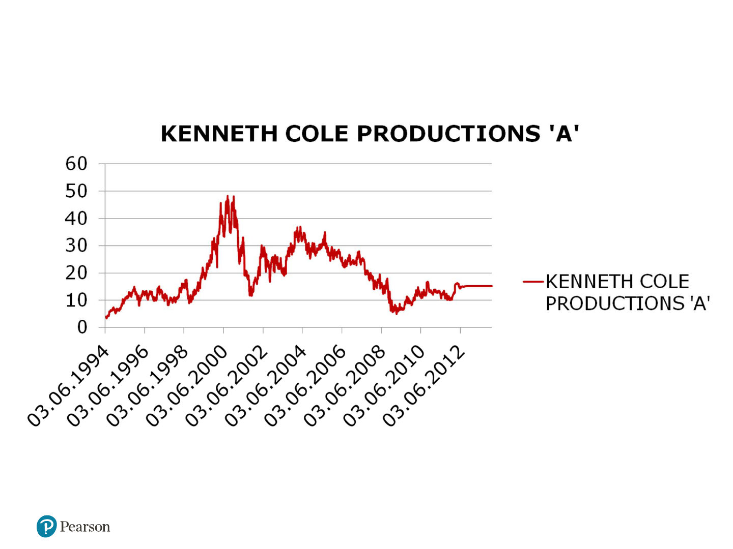
Textbook Example 9.7 (1 of 3)

Valuing Kenneth Cole Using Free Cash Flow

Problem

– Kenneth Cole (K C P) had sales of $518 million in 2005. Suppose you

expect its sales to grow at a 9% rate in 2006, but that this growth rate will

slow by 1% per year to a long –run growth rate for the apparel industry of

4% by 2011. Based on K C P ’s past profitability and investment needs, you

expect E B I Tto be 9% of sales, increases in net working capital

requirements to be 10% of any increase in sales, and net investment

(capital expenditures in excess of depreciation) to be 8% of any increase

in sales. If K C Phas $100 million in cash, $3 million in debt, 21 million

shares outstanding, a tax rate of 37%, and a weighted average cost of

capital of 11%, what is your estimate of the value of K C P ’s stock in early

2006?

Kenneth Cole Stock Price

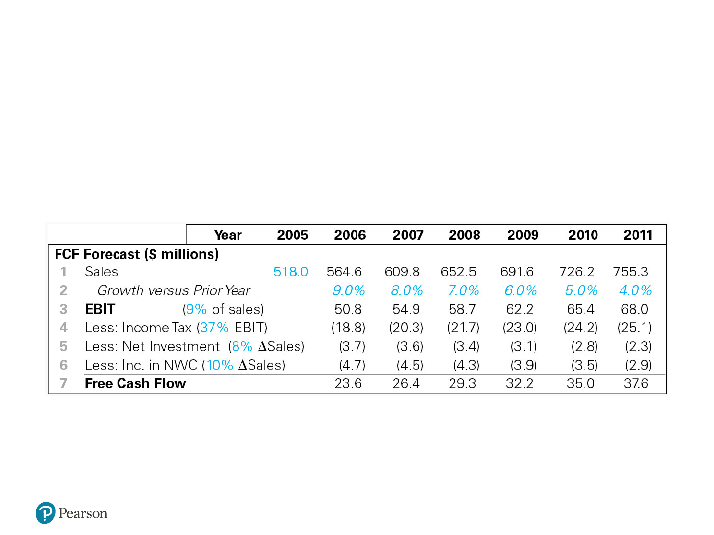
Textbook Example 9.7 (2 of 3)

Solution

Using Eq. 9.20, we can estimate K C P ’s future free cash flow

based on the estimates above as follows:

Because we expect KCP’s free cash flow to grow at a constant

rate after 2011, we can use Eq. 9.24 to compute a terminal

enterprise value:

Textbook Example 9.7 (3 of 3)

2011 2011

1+

1.04

× × 37.6 $558.6 million

0.11 0.04

FCF

wacc FCF

g

VFCF

rg











From Eq. 9.23, K C P ’s current enterprise value is the present

value of its free cash flows plus the terminal enterprise

value:

0

2345 6

23.6 26.4 29.3 32.2 35.0 37.6 + 558.6

$424.8 million

1.11 1.11 1.11 1.11 1.11 1.11

V      

We can now estimate the value of a share of K C P ’s stock

using Eq. 9.22:

0

424.8 +100 3

$24.85

21

P





The Discounted Free Cash Flow Model (5 of 5)

• Connection to Capital Budgeting

– The firm’s free cash flow is equal to the sum of the free

cash flows from the firm’s current and future

investments, so we can interpret the firm’s enterprise

value as the total N P V that the firm will earn from

continuing its existing projects and initiating new ones.

 The N P V of any individual project represents its

contribution to the firm’s enterprise value. To

maximize the firm’s share price, we should accept

projects that have a positive N P V.

Textbook Example 9.8 (1 of 3)

Sensitivity Analysis for Stock Valuation

Problem

In example 9.7, K C P ’s revenue growth rate was assumed to

be 9% in 2006, slowing to a long term growth rate of 4%.

How would your estimate of the stock’s value change if you

expected revenue growth of 4% from 2006 on? How would it

change if in addition you expected E B I T to be 7% of sales,

rather than 9%?

t

0

t

1

T

2

… 

V

0

= ? FCF

06

FCF

06

(1 + g) … FCF

06

(1 + g)

( -1)

Textbook Example 9.8 (2 of 3)

Solution

With 4% revenue growth and a 9% E B I T margin, K C P will have

2006 revenues of 518 × 1.04 = $538.7 million, and E B I T of

9%(538.7) = $48.5 million. Given the increase in sales of 538.7 −

518.0 = $20.7 million, we expect net investment of 8%(20.7) =

$1.7 million and additional net working capital of 10%(20.7) = $2.1

million. Thus, K C P ’s expected F C F in 2006 is

06

= 48.5(1 0.37) 1.7 2.1 = $26.8millionFCF 

Because growth is expected to remain constant at 4%, we can

estimate K C P ’s enterprise value as a growing perpetuity:

0

$26.8

= = $383million

(0.11 0.04)

V



Textbook Example 9.8 (3 of 3)

for an initial share value of

0

(383+100 3)

= = $22.86.

21

P



Thus, comparing this result with that of Example 9.7, we see that a

higher initial revenue growth of 9% versus 4% contributes about $2 to the

value of K C P ’s stock.

If, in addition, we expect K C P ’s E B I Tmargin to be only 7%, o u r F C F

estimate would decline to

06

= (.07 × 538.7)(1 .37) 1.7 2.1 = $20.0 millionFCF 

for an enterprise value of

0

$20

= = $286 million

(0.11 0.04)

V



and a share

value of

0

(286 +100 3)

= = $18.24.

21

P



Thus, we can see that maintaining an E B I Tmargin of 9%versus 7%

contributes more than $4.50 to K C P ’s stock value in this scenario.

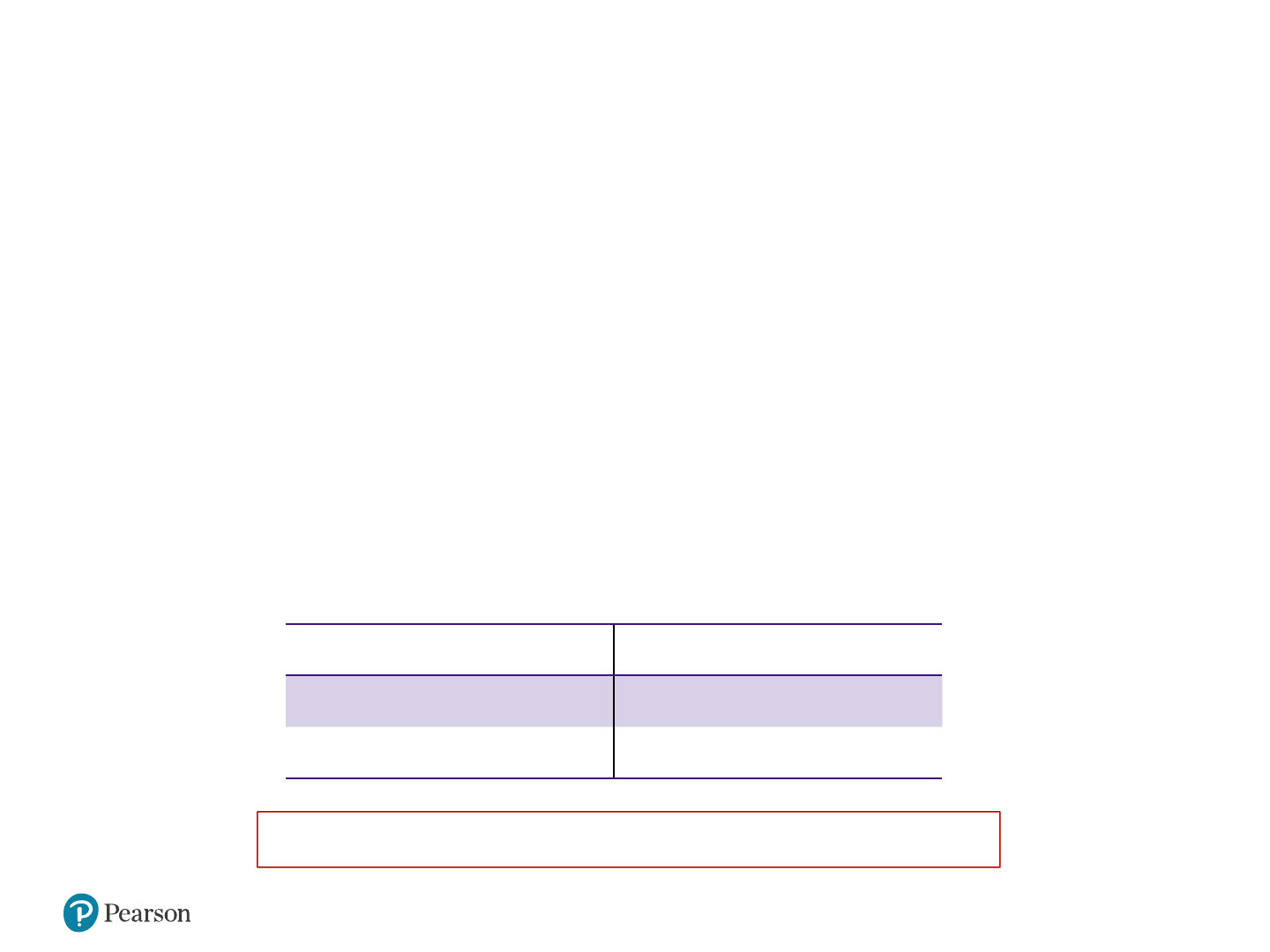
Figure 9.1 A Comparison of Discounted

Cash Flow Models of Stock Valuation

Present value of… At the … Determines the..

Dividend Payments Equity cost of capital Stock Price

Total Payouts (All dividends

and repurchases)

Equity cost of capital Equity Value

Free Cash Flow (Cash

available to pay all security

holders)

Weighted average cost

of capital

Enterprise Value

9.4 Valuation Based on Comparable

Firms

• Method of Comparables (Comps)

– Estimate the value of the firm based on the value of

other, comparable firms or investments that we expect

will generate very similar cash flows in the future

Valuation Multiples (1 of 5)

• Valuation Multiple

– A ratio of firm’s value to some measure of the firm’s

scale or cash flow

• The Price-Earnings Ratio

– P/E Ratio

 Share price divided by earnings per share

Valuation Multiples (2 of 5)

• Trailing Earnings

– Earnings over the last 12 months

• Trailing P/E

• Forward Earnings

– Expected earnings over the next 12 months

• Forward P/E

Valuation Multiples (3 of 5)

0

11

1

/

Dividend Payout Rate

Forward

EE

P

Div EPS

PE

EPS rg rg

 



/

• If two stocks have the same payout and EPS growth rates,

as well as equivalent risk (r

E

), then they should have the

same P/E.

• Firms with high growth rates, and which generate cash

well in excess of their investment needs so that they can

maintain high payout rates, should have high P/E multiples

gr

Div

P

E





1

0

:Note

Textbook Example 9.9 (1 of 2)

Valuation Using the Price-Earnings Ratio

Problem

Suppose furniture manufacturer Herman Miller, Inc., has

earnings per share of $1.99. If the average P/E of

comparable furniture stocks is 24.6, estimate a value for

Herman Miller using the P/E as a valuation multiple. What

are the assumptions underlying this estimate?

Textbook Example 9.9 (2 of 2)

Solution

We estimate a share price for Herman Miller by multiplying

its EPS by the P/E of comparable firms. Thus, P

0

= $1.99 ×

24.6 = $48.95. This estimate assumes that Herman Miller

will have similar future risk, payout rates, and growth rates to

comparable firms in the industry.

Valuation Multiples (4 of 5)

• Enterprise Value Multiples

– This valuation multiple is higher for firms with high

growth rates and low capital requirements (so that free

cash flow is high in proportion to E B I T D A)

FCFwaccFCFwacc

gr

EBITDAFCF

EBITDAgr

FCF

EBITDA

V









11

1

0

/1

Textbook Example 9.10 (1 of 2)

Valuation Using an Enterprise Value Multiple

Problem

Suppose Rocky Shoes and Boots (R C K Y ) has earnings per

share of $2.30 and E B I T D Aof $30.7 million. R C K Y also has

5.4 million shares outstanding and debt of $125 million (net

of cash). You believe Deckers Outdoor Corporation is

comparable to RCKY in terms of its underlying business, but

Deckers has little debt. If Deckers has a P/E of 13.3 and an

enterprise value to E B I T D Amultiple of 7.4, estimate the

value of R C K Y ’s shares using both multiples. Which

estimate is likely to be more accurate?

Textbook Example 9.10 (2 of 2)

Solution

Using Decker’s P/E, we would estimate a share price for

R C K Y of P

0

= $2.30 × 13.3 = $30.59. Using the enterprise

value to E B I T D Amultiple, we would estimate R C K Y ’s

enterprise value to be V

0

= $30.7 million × 7.4 = $227.2

million. We then subtract debt and divide by the number

of shares to estimate R C K Y ’s share price:

0

(227.2 125)

$18.93.

5.4

P





Because of the large difference in leverage between the

firms, we would expect the second estimate, which is based

on enterprise value, to be more reliable.

Valuation Multiples (5 of 5)

• Other Multiples

– Multiple of sales

– Price to book value of equity per share

– Enterprise value per subscriber

 Used in cable TV industry

Limitations of Multiples

• When valuing a firm using multiples, there is no clear

guidance about how to adjust for differences in expected

future growth rates, risk, or differences in accounting

policies

• Comparables only provide information regarding the value

of a firm relative to other firms in the comparison set

– Using multiples will not help us determine if an entire

industry is overvalued

Comparison with Discounted Cash

Flow Methods

• Discounted cash flows methods have the advantage that

they can incorporate specific information about the firm’s

cost of capital or future growth

– The discounted cash flow methods have the potential

to be more accurate than the use of a valuation

multiple

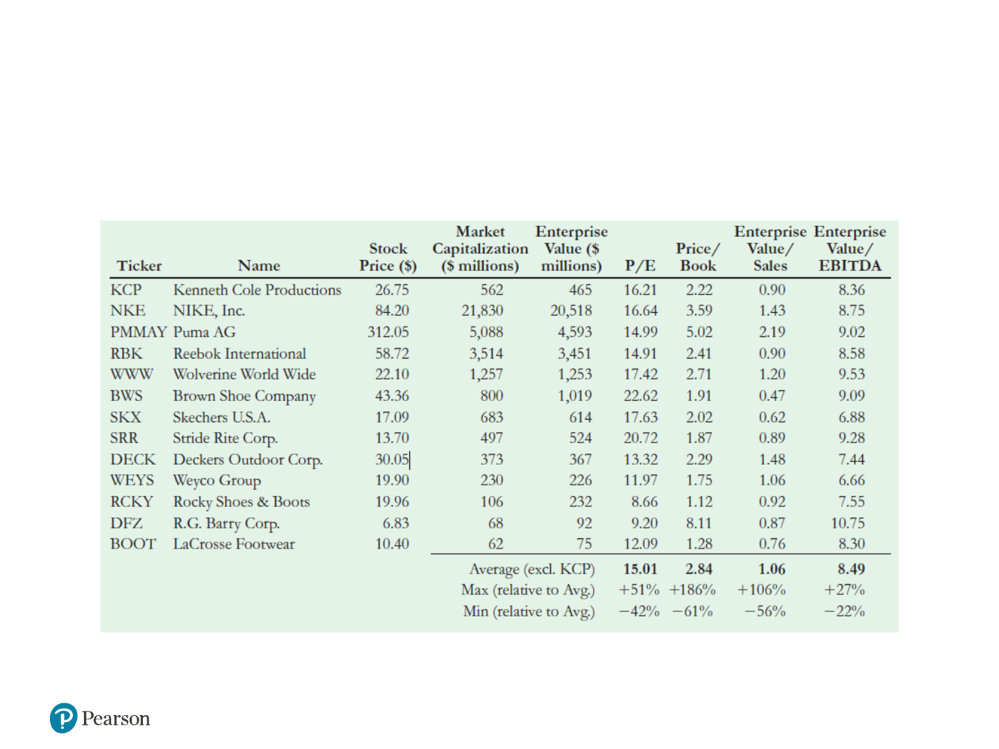
Table 9.1 Stock Prices and Multiples for

the Footwear Industry, January 2006

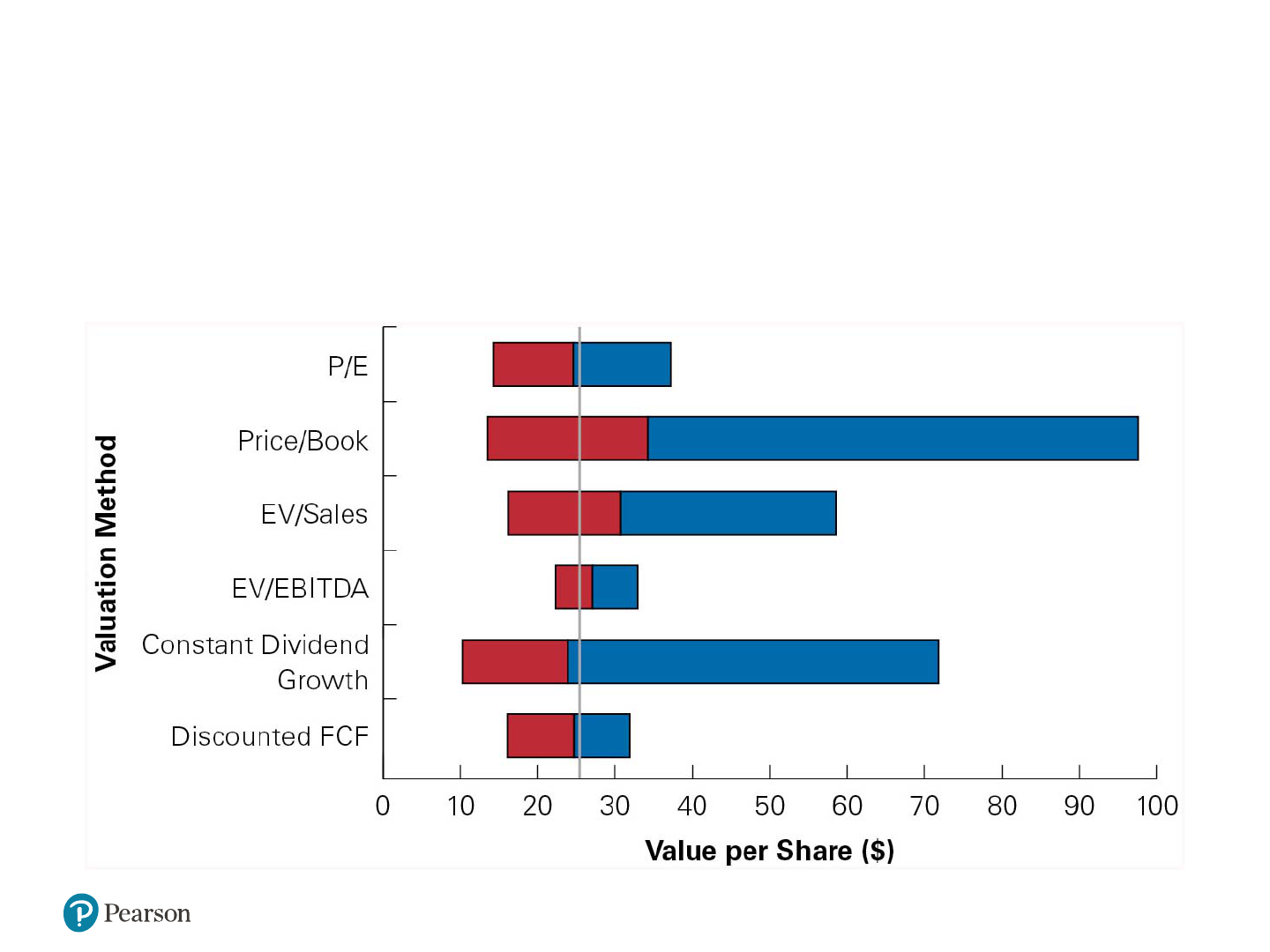
Stock Valuation Techniques: The Final

Word

• No single technique provides a final answer regarding a

stock’s true value

• All approaches require assumptions or forecasts that are

too uncertain to provide a definitive assessment of the

firm’s value

– Most real-world practitioners use a combination of

these approaches and gain confidence if the results

are consistent across a variety of methods

Figure 9.2 Range of Valuations for KCP

Stock Using Alternative Valuation

Methods

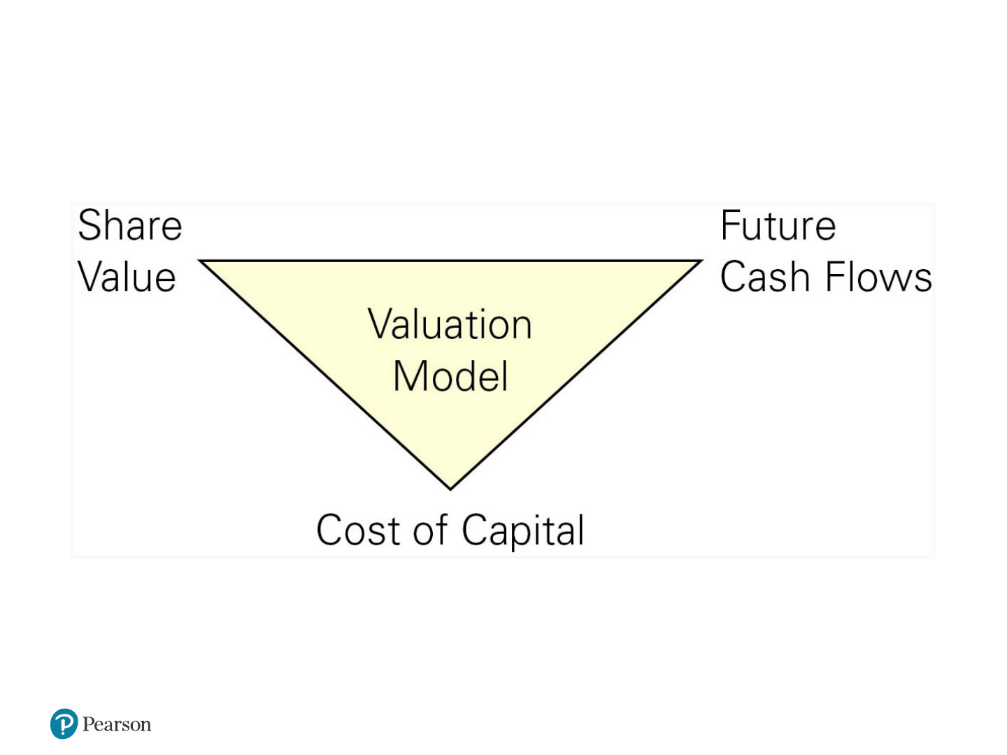
9.5 Information, Competition, and Stock

Prices

(1 of 2)

• Information in Stock Prices

– Our valuation model links the firm’s future cash flows,

its cost of capital, and its share price

– Given accurate information about any two of these

variables, a valuation model allows us to make

inferences about the third variable

Figure 9.3 The Valuation Triad

9.5 Information, Competition, and Stock

Prices

(2 of 2)

• Information in Stock Prices

– For a publicly traded firm, its current stock price should

already provide very accurate information, aggregated

from a multitude of investors, regarding the true value

of its shares

 Based on its current stock price, a valuation model

will tell us something about the firm’s future cash

flows or cost of capital

Textbook Example 9.11 (1 of 2)

Using the Information in Market Prices

Problem

Suppose Tecnor Industries will pay a dividend this year of $5

per share. Its equity cost of capital is 10%, and you except

its dividends to grow at a rate of about 4% per year, though

you are somewhat unsure of the precise growth rate. If

Tecnor’s stock is currently tradings for $76.92 per share, how

would you update your beliefs about its dividend growth

rate?

Textbook Example 9.11 (2 of 2)

Solution

If we apply the constant dividend growth model based on a 4% growth

rate, we would estimate a stock price of

0

5

$83.33 per share.

(0.10 0.04)

P 



The market price of $76.92,

however, implies that most investors except dividends to grow at a

somewhat slower rate. If we continue to assume a constant growth rate,

we can solve for the growth rate consistent with the current market price

using Eq. 9.7:

1

0

5

10% 3.5%

76.92

E

Div

gr

P

   

Thus, given this market price for the stock, we should lower our

expectations for the dividend growth rate unless we have very strong

reasons to trust our own estimate.

Competition and Efficient Markets

(1of 4)

• Efficient Markets Hypothesis

– Implies that securities will be fairly priced, based on

their future cash flows, given all information that is

available to investors.

Competition and Efficient Markets

(2 of 4)

• Public, Easily Interpretable Information

– If the impact of information that is available to all

investors (news reports, financials statements, etc.)

on the firm’s future cash flows can be readily

ascertained, then all investors can determine the

effect of this information on the firm’s value

 In this situation, we expect the stock price to react

nearly instantaneously to such news

Textbook Example 9.12 (1 of 2)

Stock Price Reactions to Public Information

Problem

Myox labs announces that due to potential side effects, it is

pulling one of its leading drugs from the market. As a result,

its future excepted free cash flow will decline by $85 million

per year for the next 10 years. Myox has 50 million shares

outstanding, no debt, and equity cost of capital of 8%. If this

news came as a complete surprise to investors, what should

happen to myox’s stock price upon the announcement?

Textbook Example 9.12 (2 of 2)

Solution

In this case, we can use the discounted free cash flow method.

With no debt, Using the annuity formula, the decline

in expected free cash flow will reduce Myox’s enterprise value by

==8%.

wacc E

rr

10

11

$85 million × 1 $570 million

0.08 1.08









Thus, the share price should fall by

$570

$11.40 per share.

50



Because this news is public and its effect on the firm’s expected

free cash flow is clear, we would expect the stock price to drop by

this amount nearly instantaneously.

time

Stock

price

11.40

Competition and Efficient Markets

(3 of 4)

• Private or Difficult-to-Interpret Information

– Private information will be held by a relatively small

number of investors

– These investors may be able to profit by trading on

their information

 In this case, the efficient markets hypothesis will not

hold in the strict sense

 However, as these informed traders begin to trade,

they will tend to move prices, so over time prices will

begin to reflect their information as well

Competition and Efficient Markets

(4 of 4)

• Private or Difficult-to-Interpret Information

– If the profit opportunities from having private

information are large, others will devote the resources

needed to acquire it

 In the long run, we should expect that the degree of

“inefficiency” in the market will be limited by the

costs of obtaining the private information

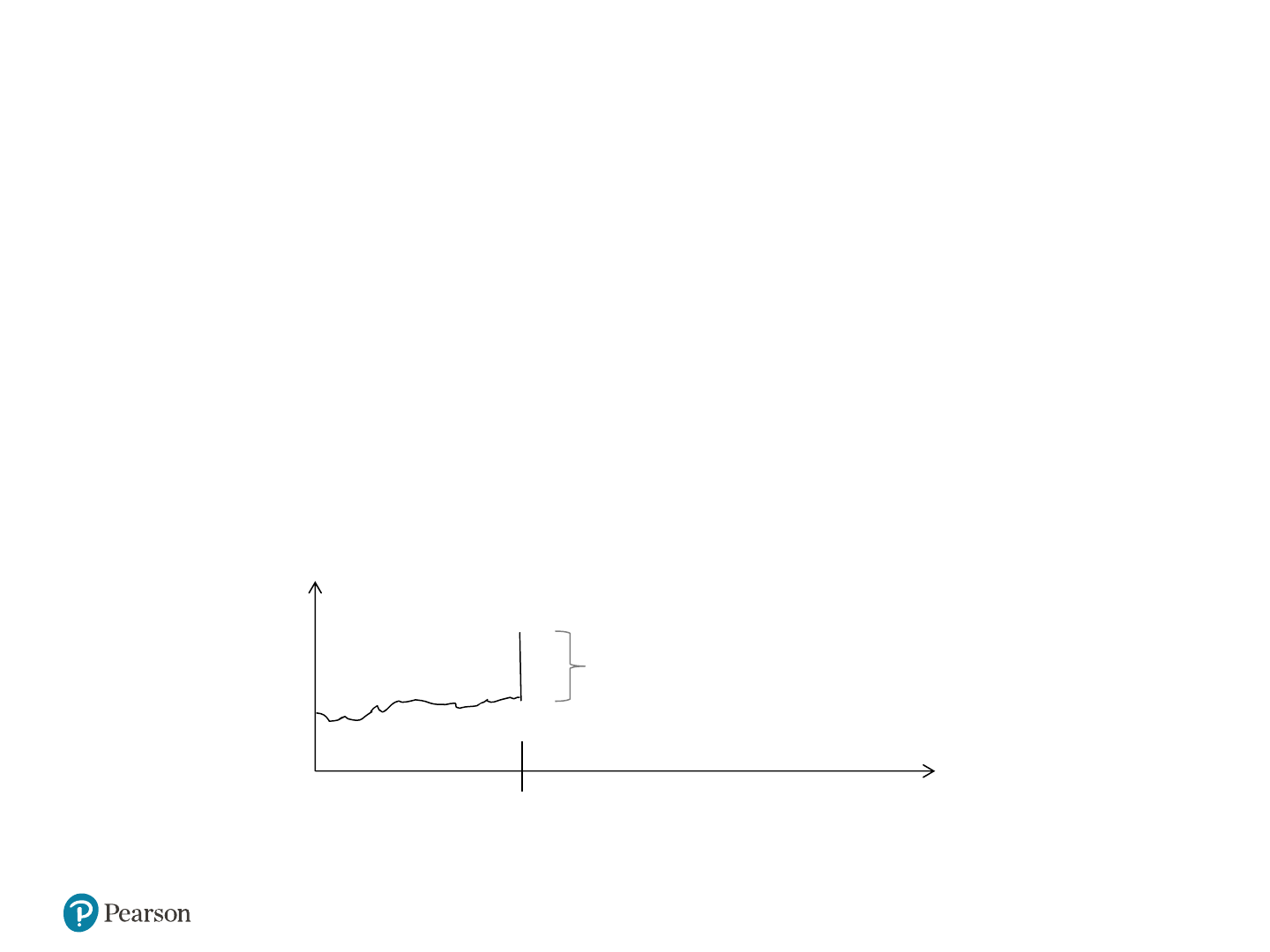
Textbook Example 9.13 (1 of 2)

Stock Price Reactions to Private Information

Problem

Phenyx Pharmaceuticals has just announced the development of a new

drug for which the company is seeking approval from the Food and Drug

Administration (F D A). If approved, the future profits from the new drug

will increase Phenyx’s market value by $750 million, or $15 per share

given its 50 million shares outstanding. If the development of this drug

was a surprise to investors, and if the average likelihood of F D Aapproval

is 10%, what do you expect will happen to Phenyx’s stock price when

this news is announced? What may happen to the stock price over time?

time

Stock

price

$1.50

announcement

date

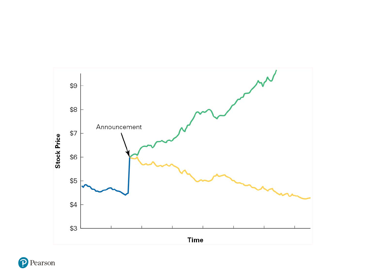
Textbook Example 9.13 (2 of 2)

Solution

Because many investors are likely to know that the chance of F D A

approval is 10%, competition should lead to an immediate jump in the

stock price of 10% × $15 = $1.50 per share. Over time, however,

analysts and experts in the field are likely to do their own assessments of

the probable efficacy of the drug. If they conclude that the drug looks

more promising than average, they will begin to trade on their private

information and buy the stock, and the price will tend to drift higher over

time. If the experts conclude that the drug looks less promising than

average, they will tend to sell the stock, and its price will drift lower over

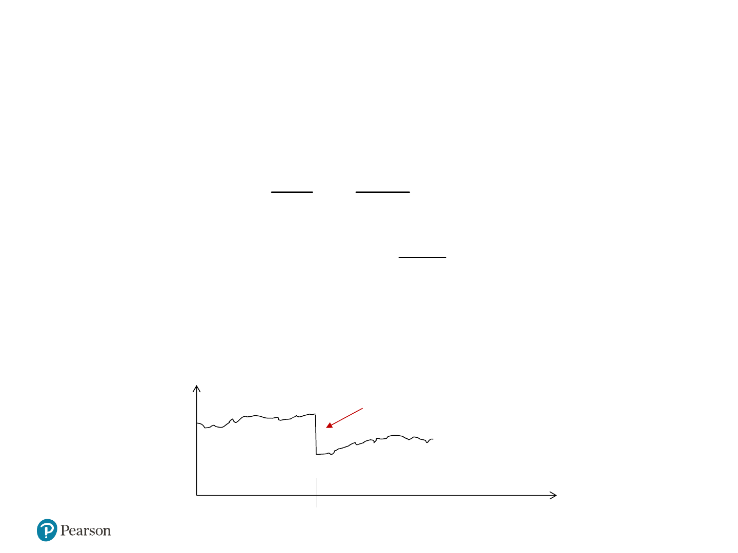
time. Examples of possible price paths are shown in Figure 9.4. While

these experts may be able to trade on their superior information and earn

a profit, for uninformed investors who do not know which outcome will

occur, the stock may rise or fall and so appears fairly priced at the

announcement.

Figure 9.4 Possible Stock Price Paths

for Example 9.13

Lessons for Investors and Corporate

Managers

(1 of 2)

• Consequences for Investors

– If stocks are fairly priced, then investors who buy

stocks can expect to receive future cash flows that

fairly compensate them for the risk of their investment

 In such cases, the average investor can invest with

confidence, even if he is not fully informed

Lessons for Investors and Corporate

Managers

(2 of 2)

• Implications for Corporate Managers

– Focus on N P V and free cash flow

– Avoid accounting illusions

– Use financial transactions to support investment

The Efficient Markets Hypothesis

Versus No Arbitrage

• The efficient markets hypothesis states that securities with

equivalent risk should have the same expected return

• An arbitrage opportunity is a situation in which two

securities with identical cash flows have different prices

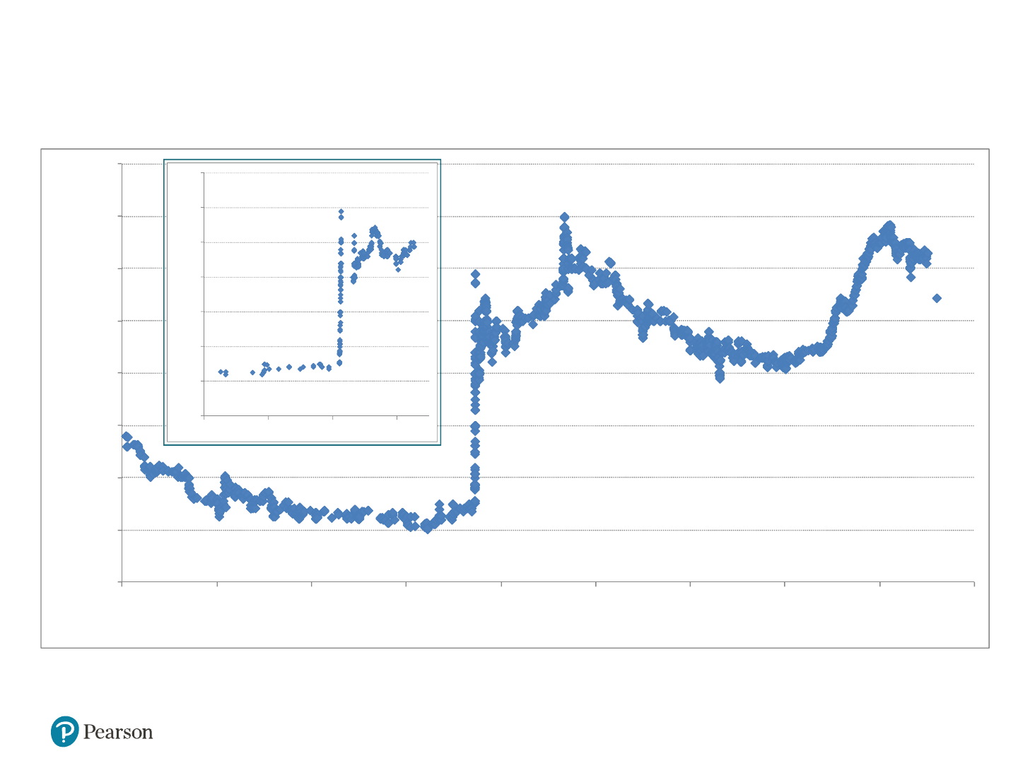
ACS bid for Hochtief

63

63,5

64

64,5

65

65,5

66

66,5

67

9

10

11

12

13

14

15

16

17

18

Aktienkurs in EUR

Uhrzeit

63

63,5

64

64,5

65

65,5

66

66,5

12,

3

12,

5

12,

7

12,

9

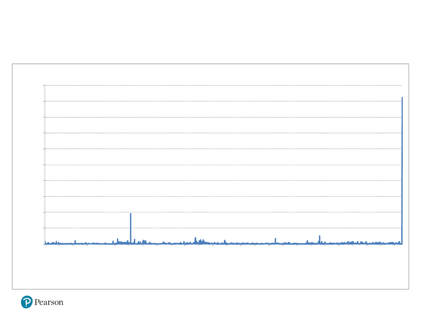
Hochtief Trading Volume XETRA

0

10000

20000

30000

40000

50000

60000

70000

80000

90000

100000

09.02.10,00

09.42.03,67

10.11.27,69

10.52.07,29

11.29.55,25

12.29.13,36

12.43.31,89

12.47.39,50

12.50.14,31

12.55.19,33

13.13.33,22

13.39.29,07

13.50.20,06

14.15.49,19

14.34.23,82

15.04.54,35

15.14.05,48

15.16.59,55

15.35.17,12

15.59.39,58

16.09.06,51

16.26.31,12

16.42.01,29

16.52.25,36

17.07.07,60

17.22.26,46

Volumen

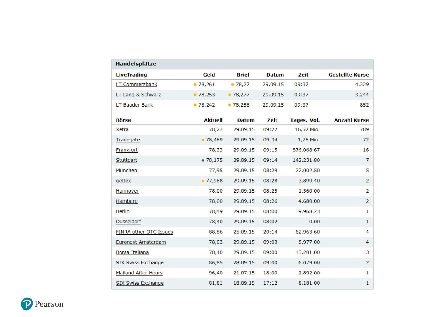
Stock Exchanges in Germany

Siemens

Sep 29

2015

9:38 a.m.

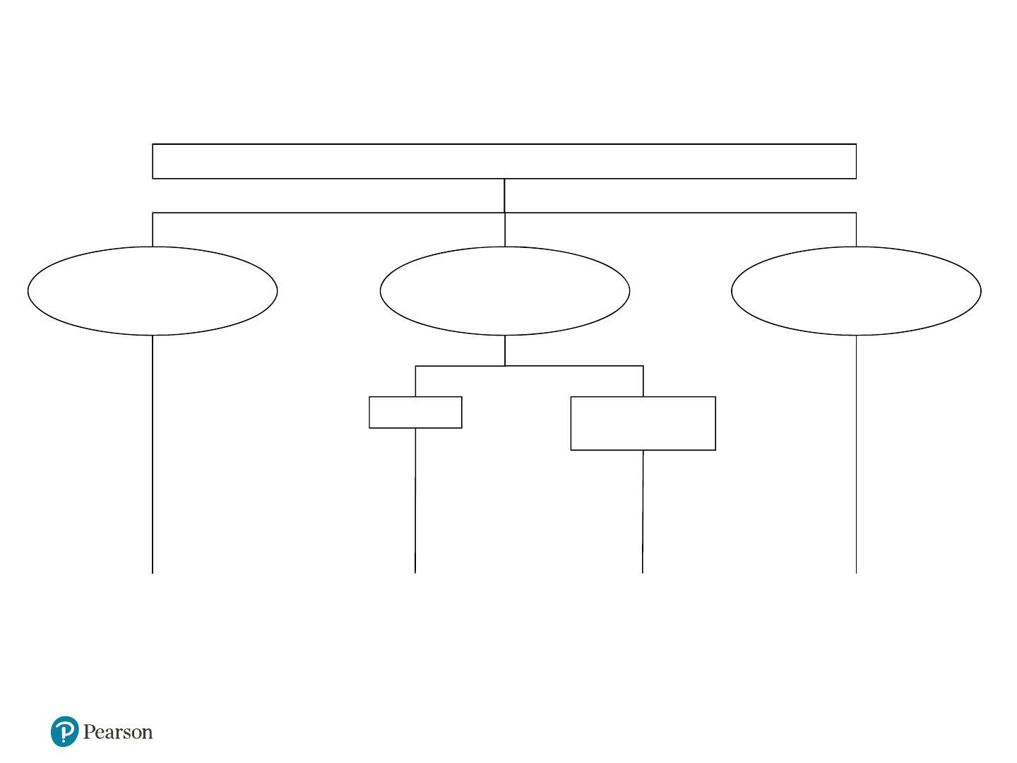
Stock Trading overview

Nationaler Aktienhandel (Kassamarkt)

Parketthandel

Elektronischer Handel

Telefonhandel

börslich außerbörslich

(ATS/ECN)

Regionalbörsen XETRA,

Frankfurt

Tradegate Handel zw.

Institutionelle

n

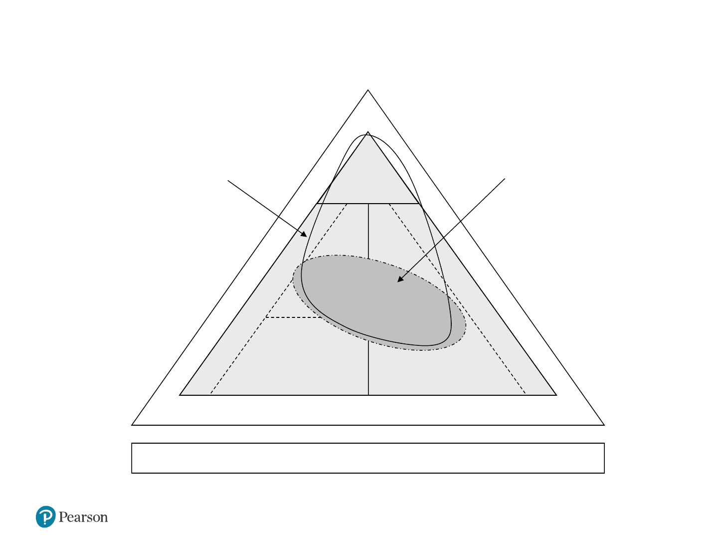
Indexes after Sep. 24 2018

Prime Standard

General Standard

DAX

(30)

SDAX

(70)

TecDAX

(30)

MDAX

(60)

Midcap Market-Index

(60 - 90)

HDAX

(90 - 120)

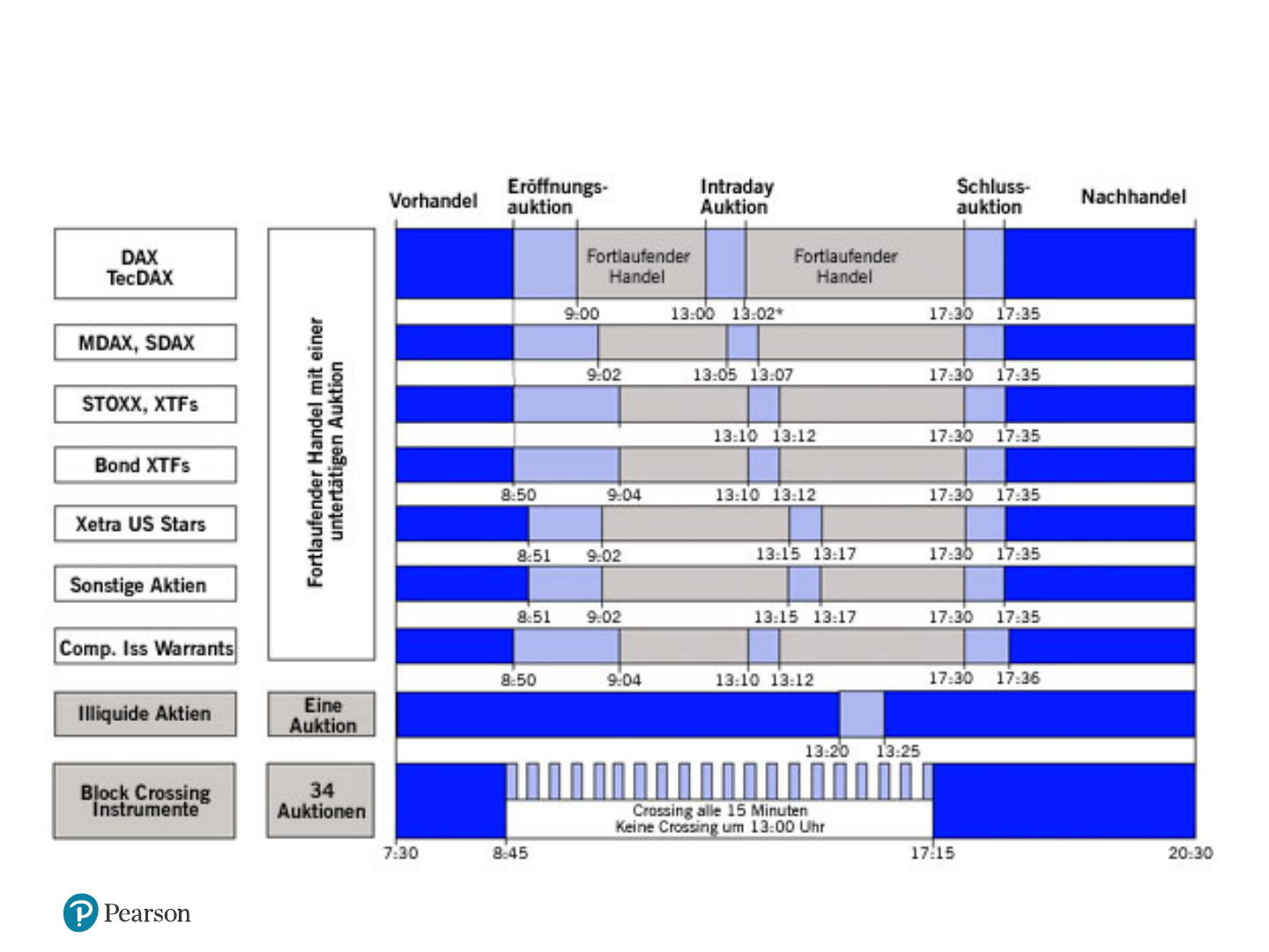
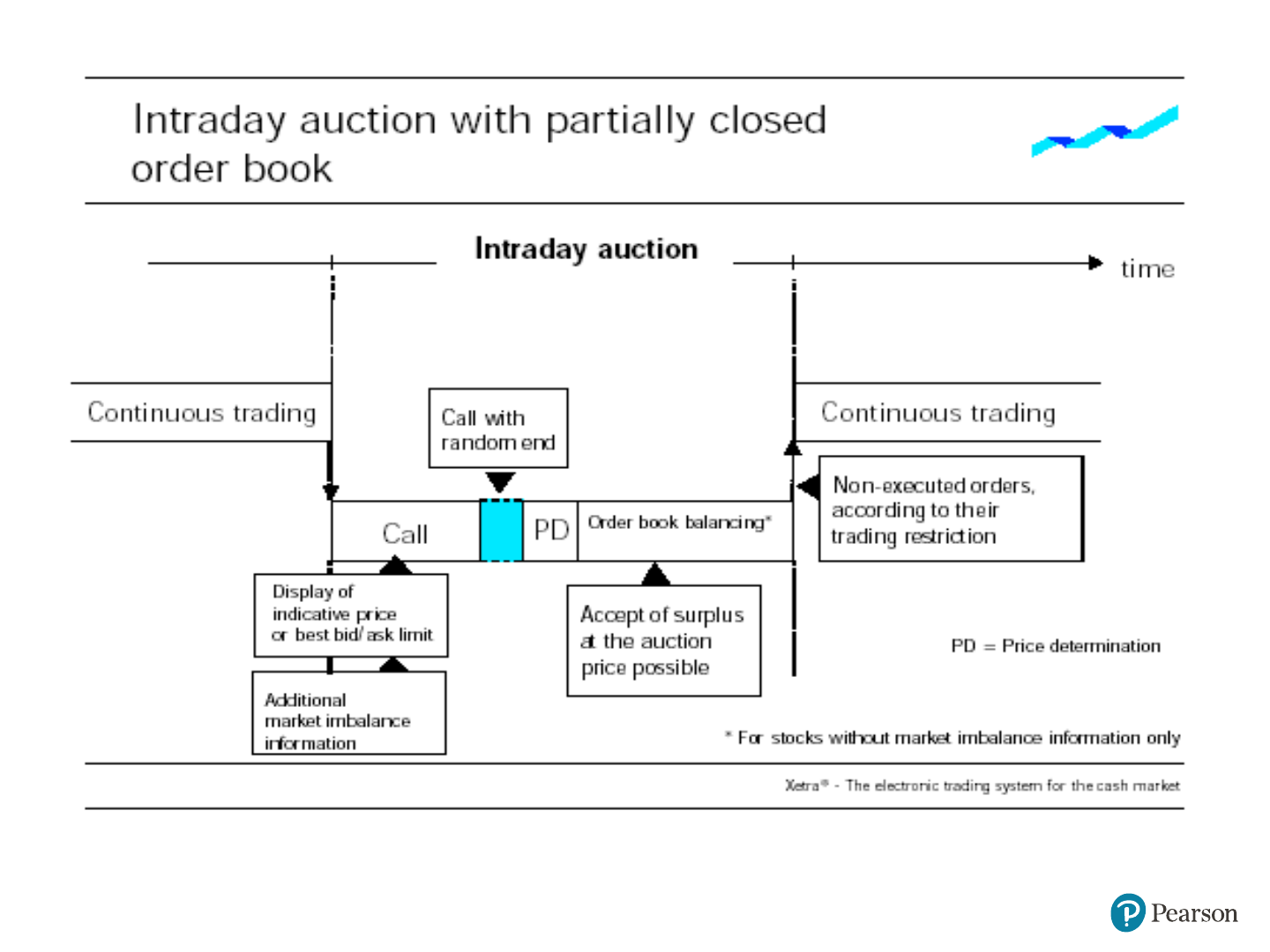
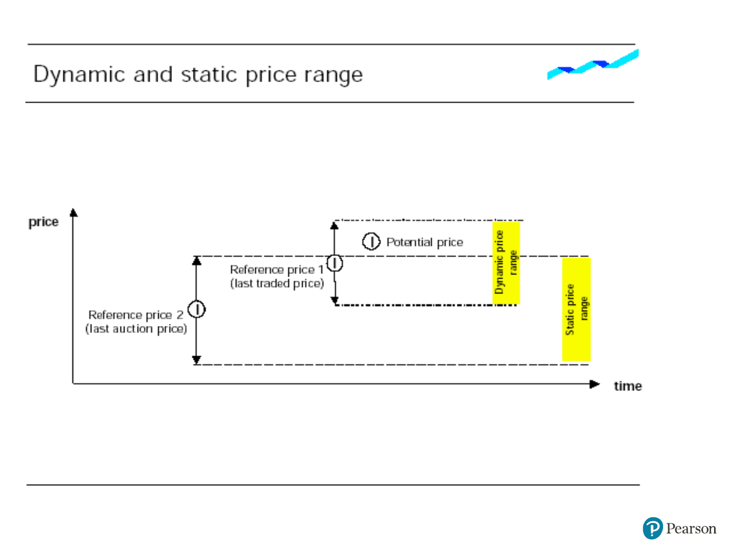
Trading Time XETRA

Floor Trading

8 Uhr

22 Uhr

Opening auction

End of trading

Continuous trading

German Stocks since 1870 nominal

100

1000

10000

100000

1E+06

1E+07

1E+08

1E+09

1E+10

1E+11

1E+12

1E+13

1E+14

1E+15

1870

1880

1890

1900

1910

1920

1930

1940

1950

1960

1970

1980

1990

2000

2010

German Stocks real values

100

1000

10000

100000

1870

1880

1890

1900

1910

1920

1930

1940

1950

1960

1970

1980

1990

2000

2010