Chapter 22: Statistical Data Analysis
22.1- Introduction
22.2 - Types of Error
Gross Error
Systematic Error
Random Error
22.3 - Precision vs. Accuracy
22.4 - Statistical Tools
Population vs. Sample
Mean
Standard Deviation and Variance
Standard Error and Error Bars.
Normal Distributions
Confidence Limits
Using Spreadsheets to Determine Confidence Limits
Propagation of Error
Analyzing Data Sets
Identifying Outliers: The Q-Test
Identifying Outliers: The Grubb’s Test
Analyzing Variance: The F-Test
ANOVA: A 2-Dimenstional F-Test
22.5 - Linear Regression Analysis
22.6 - LOD, LOQ and LDR
22.7 - Further Reading
22.8 - Additional Exercises
671

22.1 - Introduction
When we make an instrumental measurement, we want the measurement to be “correct.” So
it makes sense for us to start this discussion with a look at what the word “correct” means to a
scientist. When we make a measurement, there is a fundamental limit to how well we can
“know” the answer
1
. Therefore a real measurement cannot have a single “true” value and to
be complete, must be accompanied by a statement of the uncertainty in the number. In order
for a scientific measurement to be “correct” it must represent the best estimate of the mean of
a set of replicate measurements and be accompanied by an estimate of the uncertainty in the
mean (i.e. error). For example you might see a reported mass as 2.15 ±0.01 grams. The typical
interpretation of this reported value would be that our best estimate of the “true” value is 2.15
grams and the standard deviation of the mean lies in the range of 0.01 above and below the
value of 2.15. Unfortunately the interpretation of the ±0.01 is not consistent throughout all
disciplines of science. Although we have stated here that the ±0.01 typically represents
standard deviation, it is possible that the ±0.01 represents the standard error or the confidence
interval
2
. It is a best practice to always include a statement describing how you are reporting
error in all of your scientific reports.
22.2 - Types of Error
“Nature does not give up her secrets lightly
3
” and in the pursuit of
nature’s secrets it is accepted that the first measurement will yield a false representation of the
truth. In other words, any single data point will inherently contain error
4
. The word error
comes from Latin and loosely translates as “wandering.” For our purposes we define error as
the difference between the experimentally obtained value and the true value. Ironically, if we
knew the true value, we would have no need to conduct the experiment in the first place. This
leads us to a philosophically important conclusion. The goal of an experiment is to obtain a
“true” measured value but since all measured data points contain error, we can never know
with absolute certainty the true value of an experimentally obtained result. All experimentally
obtained results contain uncertainty. Therefore, it is the analyst’s objective to minimize and
quantify error.
It is generally recognized that there are three broad categories of error; gross error,
5
systematic
error
6
and random error.
1
This implied by the Heisenberg Uncertainty Principle: Werner Heisenberg. Z. Phys. 43 (3–4): 172–198. 1927
2
We will define standard error and confidence limits later in this chapter.
3
Brian Greene, The Fabric of the Cosmos: Space, Time, and the Texture of Reality, First Vintage Books (2004)
4
We will use the terms uncertainty and error interchangeably.
5
Also known as human error, operator error, or illegitimate error.
6
Also known as bias.
It is the analyst’s
objective to minimize
and quantify error.
672

Gross Error
Gross error occurs when the analyst makes a mistake. For example the analyst might misread a
balance or strike the wrong button on his/her calculator. These gross errors are often obvious.
However not all mistakes are treated equal. For example, if you were to make replicate
measurements of the volume of your favorite coffee mug and you obtained a set of volumes
such as 298 ml, 302 ml, 299 ml, 80.53 liters, 297 ml, 301 ml, 299ml, 295 ml, 301 ml and 270 ml,
you would immediately recognize that the 80.53 liter measurement was completely WRONG.
You obviously made a mistake! The purist might say that you must keep the 80.53 liter data
point until you can statistically justify the exclusion of that data point. However in practice few
analysts will keep a data point if it is completely obvious that a gross mistake was made. But be
careful. Casually throwing out data points that you do not like is against best practices. There
are good reasons why the purist will always justify an exclusion using statistical tools. Taking
another look at our data you might also wonder about the 270 ml data point? If you exclude
the 80.53 liter data point AND the 270 ml data point you get an average value of 299 ml. It
would appear that the 270 ml data point is ≈ 30 ml “too low”. You might be tempted to ignore
that data point but again, this would be a violation of best practices and in this case it is not so
obvious that the answer is WRONG. Within the precision of your technique, the 270 ml data
point might be legitimate. For example, if you keep the 270 ml data point, you obtain an
average of 295.7 ml and your original data set had a data point of 295 ml. By casually throwing
out the 270 ml data point, you may have artificially raised the mean of your data set. You
would first need to statistically justify the exclusion of the 270 ml data point before you could
ignore it. Data points that statistically fall outside the range of a data set are called outliers.
We will explore the notion of outliers further in section 22.4 when we discuss Q-tests and
Grubb’s-tests.
Systematic Error
Systematic error can be described as a measurement that is always too high or always too low,
and the magnitude of the deviation from the “true” value is constant. Systematic error is often
difficult to identify. The origin of systematic error can be chemical and/or instrumental in
origin. Instrumental systematic errors can result from drift noise
7
, external interference, or
improper calibration of the instrument. For instance an improper ground wire may result in a
bias on the detector that artificially raises or lowers the instrument response to your
measurement. Likewise, if your instrument’s critical components are not properly shielded, an
external magnetic or radio frequency signal can cause your instrument’s response to shift from
its original calibrated value. Instrumental systematic errors are identified by analyzing carefully
constructed standards on a regular basis. For example, baseline drift is a common problem
when conducting AAS analysis. For this reason it is common for AAS methods to incorporate a
blank and a known standard in the analysis after every 5 or 10 samples.
Chemical systematic error occurs in many ways. For instance any error in the construction of
standards used to calibrate an instrument will necessarily impart a systematic error to the
instrumental response. Or a chemical systematic error might result from chemical steps used in
7
See Chapter 5 for a review of noise sources.
673
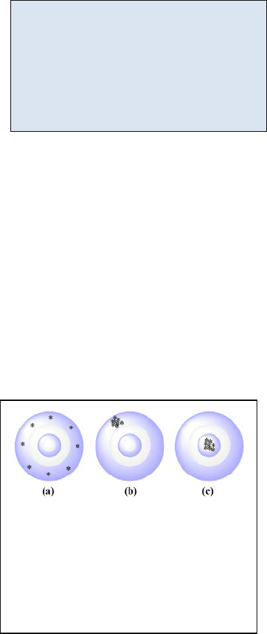
Figure 22.1: Three targets. Target (a)
has relatively high accuracy but
relatively low precision. Target (b)
has relatively low accuracy but
relatively high precision. Target (c)
has relatively high accuracy and
relatively high precision.
preparing the sample for analysis. For example, it is common to esterify carboxylic acids prior
to GC/MS analysis. If the derivatization step had a yield of 85%, the analyst would need to
correct for the 15% loss, otherwise there would be a negative systematic error of 15% in the
final results. Likewise you can imagine a similar loss of sample if there was an inefficient
extraction step in the sample preparation.
Random Error
Random errors are unpredictable high and low
fluctuations in the measurement of physical properties.
These fluctuations can arise from environmental changes
such as moment to moment fluctuations in pressure or
temperature or are the result of slight variation in the
procedural steps. Fortunately, random error can be quantified using statistical tools. Absent
any gross or systematic error, if one repeats an experiment several times, the mean value of a
normally distributed data set will appear close to the true value and the scatter about the mean
can be used to quantify the confidence we have in that mean. We will discuss each of these
ideas in more detail later in this appendix.
22.3 - Precision vs. Accuracy
In the simplest case, accuracy is used to quantify the correctness of an analysis; or how close
the measured value is to the “true” value. Precision is used to quantify the reproducibility of
our technique; or how close to the previous measurements will our next measurement be? A
common analogy used when discussing the terms accuracy and precision is that of hitting a
target. In Figure 22.1 (a) we have a situation in which the reproducibility of each attempt is low
but if we average the distance of each attempt from
the bull’s eye, we get an average value very close to a
perfect bull’s eye. We would say that the precision is
low but the accuracy of the mean can be made
acceptable if enough data is collected and the results
averaged. Conversely in Figure 22.1 (b) we have a
scenario in which the reproducibility of each shot is
relatively high but the shooter consistently failed to hit
the bull’s eye. We would say that the precision is high
but the accuracy is low. Averaging these shots will not
yield a result close to the bull’s eye. Relating these
results to the previous section, we would conclude that
this shooter has a systematic error of shooting high and
to the left in addition to the random error one normally sees with target shooting. Finally in
Figure 22.1 (c) we have a scenario in which the precision and accuracy are both relatively high.
Tying these ideas together we recognize that the precision of an experiment is related to our
ability to minimize random error. In target (b) and (c) of Figure 22.1 we see relatively small
random error. They are both precise but only target (c) is also accurate. The accuracy of an
The precision of an experiment is
influenced most by
our ability to
control random error.
The accuracy
of an experiment is
influenced
most by our ability to
control systematic error.
674

experiment is related to our ability to minimize systematic error. For example, target (b) shows
a systematic error resulting in a high and right pattern resulting in an inaccurate result.
22.4 - Statistical Tools
Population vs. Sample
Before we delve too deeply into specific statistical tools, we need to define some terms. The
term population is used when an infinite sampling occurred or all possible subjects were
analyzed. Obviously we cannot repeat a measurement an infinite number of times so quite
often the idea of a population is theoretical; and in those cases we take a representative sample
of the entire population. For example, if you wanted to know the average height of the human
race, you would have to take a representative sample of people and measure their heights.
Your result would be an estimate and you would necessarily report the uncertainty of your
estimate. However, if the parameters of an experiment are specifically defined, one can
analyze an entire population. For example, if your question was “what is the average height of
your immediate family” then your population has been defined as your immediate family and it
is now possible to measure the height of the entire population. Despite your ability to collect
data on the entire population, you still have random error associated with each measurement.
Be careful to distinguish the statistical use of the word sample from the way a chemist often
uses the word “sample”. For example, if we were analyzing the soil in a field for arsenic
concentration, we might go out to the field and collect 20 representative soil “samples” and
bring them back into the lab. The 20 soil “samples” would give us 20 data points. The
statistician would call the entire set of 20 data points the sample since the 20 data points are
being used to sample the entire population. It can be a confusing tangle of words so take a
moment to think through it.
Mean
The term mean is synonymous with the term average and is obtained by summing all of the
results from an analysis and dividing by the total number of individual results (N). The symbol
for a population mean is
µ
and the symbol for a sample mean is
.
=
Eq. 22.1
=
Eq. 22.2
where
µ
i
and x
i
are the results of the i
th
experiment.
As N ∞,
µ
. How quickly
µ
is dependent upon the relative amount of random error
(precision) associated with each individual measurement, x
i
. We quantify the random error
using two statistical tools called the standard deviation and the variance.
675

Standard Deviation and Variance
The equations for calculating a standard deviation of a population and the standard deviation of
a sample are given in Equations 22.3 and 22.4. The symbol for a population standard deviation
is
σ
and the symbol for a sample standard deviation is s.
=
(
)
Eq. 22.3
=
(
)
Eq. 22.4
If we take a close look at Equations 22.3 we see that the term (x
i
-µ) is nothing more than the
deviation of an individual data point from the population mean. We then square the deviation
values for each data point to get rid of the negative sign. By summing all of the squares,
dividing by N and taking the square root we are left with an average absolute deviation. So for
a population, the standard deviation is simply the absolute value of the average deviation from
the mean. However when determining the standard deviation of a sample, we have a slight
modification to the equation. In Equation 22.4, we use (N-1) in the denominator instead of N.
The term (N-1) is defined as the degrees of freedom for a sample set. Degrees of Freedom
represent the number of repeated measurements (a.k.a. replicates) that are free to vary. Since
the mean of a sample set is constrained by the mean of the population, the last data point is
not “free to vary” since the average of all data points must represent the mean of the
population. Degrees of freedom show up in several other statistical tools so it is important that
you take a moment to learn this term.
On many calculators, the buttons for calculating standard deviation are labeled σ & σ
n-1
, where
σ
n-1
is the sample standard deviation that we have represented here with the symbol “s” as
defined in Equation 22.4. One rarely samples an entire population in a laboratory experiment
so in almost every case you will want to use Equation 22.4 or your σ
n-1
button on your
calculator to calculate “s”.
676
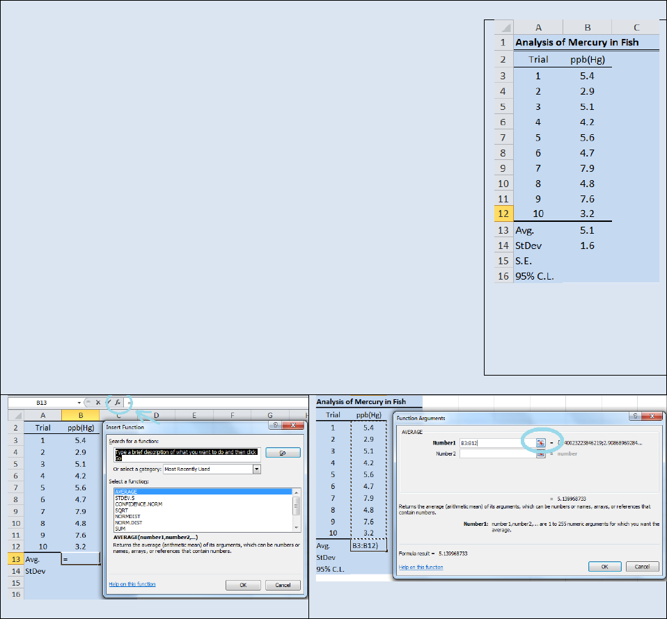
Activity – Using Excel® to generate a mean and standard deviation.
Recreate the spreadsheet seen in Figure 22.2 in Microsoft Excel®. Select
cell B13 and click on the f
x
button to open the Insert Function dialog box
(see Figure 22.3). From the drop down
window in the Insert Function
dialog box, select Statistical. And in the Select Function
window select
AVERAGE. The Function Argument dialog box will open (see Figure 22.4).
The AVERAGE function will use Equation 22.2 to calculate the average of
the data set. In the Number1 field enter the range of addresses for the
numbers you wish to average. In this example the range of addresses is
B3:B12. Or you can click the grid button (cirled in blue in Figure 22.4) and
drag and drop the range of values to be averaged.
Click OK and the
average of cells B3
B12 will be returned in cell B13. Now select cell B14
and repeat the above sequence of steps but this time select the STDEV.S
function instead of the AVERAGE function. STDEV.S uses Equation 22.4 to
calculates the standard deviation of a sample. The Function Arguments
box will open again and you will need to enter the range of values for the
data set (B3:B12) or you can use the drag and drop function. Your final
spread sheet should resemble the one shown in Figure 22.2. We will revisit
this data set when we discuss standard error and confidence limits (CL) so
take a moment to save your spreadsheet as Fish.
Figure 22.2: Spreadsheet
demonstrating the use of
Excel to calculate a mean
and a standard deviation.
Figure 22.3: Insert Function Dialog Box
Figure 22.4: Function Arguments Dialog Box.
Although the key strokes differ from calculator to calculator, most scientific calculators can
perform the statistics function we outlined in the Activity above. The steps typically involve
entering the data points into a data array (often symbolized with a Σ+ button). As you enter
each data point, the total number of points in the array will be displayed as N=#. Once you
have entered your data array, you can press the button to display the average or the σ or σ
(n-
1)
buttons to display the appropriate standard deviation.
677
Exercise 22.1: Using the same data set we examined in the above activity, use the statistical
functions on your calculator to determine the mean and the standard deviation of the data set.
You may need to review your owner’s manual or visit the manufacture’s website for
instructions on using the stats functions on your calculator.
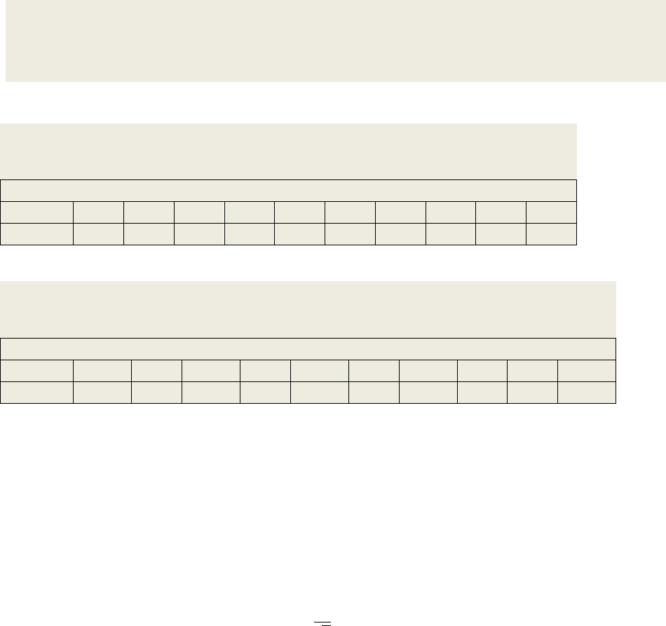
Exercise 22.2: Use Excel® or a similar spreadsheet program to determine the mean and
standard deviation of the following data sample. Repeat the analysis using your
calculator’s statistical functions.
Lead in Drinking Water
Replicate
1
2
3
4
5
6
7
8
9
10
ppm
2.002
1.996
2.000
1.995
1.999
1.987
2.010
2.014
2.007
2.004
Exercise 22.3: Use Excel® or a similar spreadsheet program to determine the mean and
standard deviation of the following data sample. Repeat the analysis using your calculator’s
statistical functions.
Lead in a Paint Chip
Replicate
1
2
3
4
5
6
7
8
9
10
ppm
1001.9
989.0
1020.4
996.1
1002.4
990.0
1019.4
991.3
999.2
1002.4
Standard Error & Error Bars
In the introduction to this chapter we reported a mass as 2.15 ±0.01 grams and mentioned that
the ±0.01 indicated one standard deviation unit above and below the mean and in our activity
above, we reported the concentration of mercury in fish flesh as 5.1 ±1.6 ppb. The
conventional way to report error graphically is to include “error bars". Chemist typically report
error using standard deviation however not all disciplines of science share the same
conventions. Another very common way to represent error is to report a value called the
standard error. The standard error is related to standard deviation as seen in Equation 22.5
. . =
Eq. 22.5
Note that for a given set of measurements, the standard error will always be less than the
standard deviation.
Excel allows the user to report error bars on a graph as either the standard deviation, standard
error, or as a percentage of the mean. Additionally, Excel allows you to add a customized value
for the error bars. It is important that you specify how you are reporting your uncertainty in
your numbers. This is appropriately done in the figure caption.
678
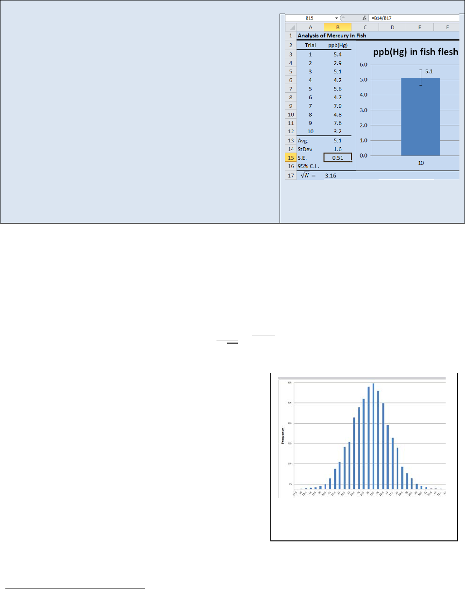
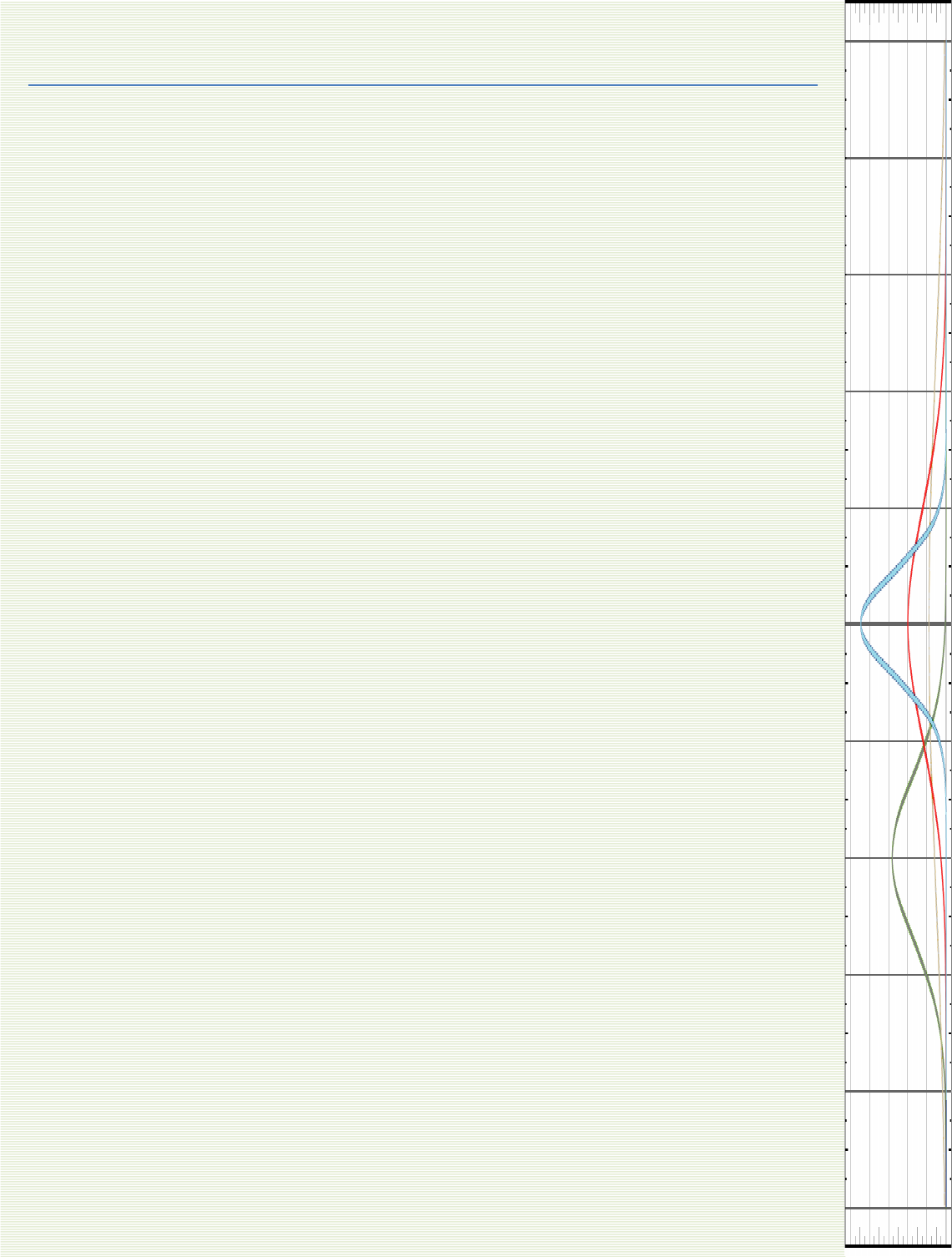
Figure 22.6: Histogram demonstrating
a normal distribution of points about a
mean:
= , = , = .
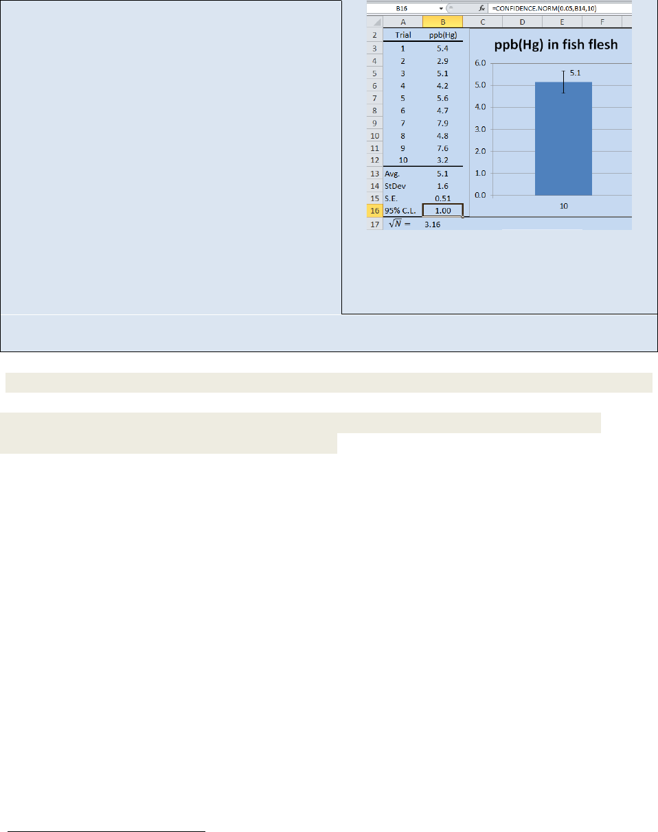
Activity – Using Excel® to calculate standard error and plotting error bars on a bar-graph.
Open the spreadsheet Fish that you created in the previous
Activity. We are going to program Eq. 22.5 for the standard
error into cell B15. First we need to calculate the square root
of N. Select cell B17 and type “=sqrt(10)”. Excel will return a
value of 3.16. Next select cell B15 and type “=B14/B17”.
Excel will return a standard error of 0.51.
To display the standard error as error bars on a graph, first
create a graph of your data. In this activity, we have created
a column graph. Next, place your cursor in the graph and
“left-click”
8
. This will display the “Chart Tools” group. From
the “Chart Tools” group, select the “Layout” tab. Next select
“Error Bars” from the “Analysis Group” and fill in the correct
parameters. Your spread sheet should now resemble the one
in Figure 22.5. We will return to this spread sheet when we
discuss confidence limits so be certain to save your work.
Figure 22.5: Determining Standard
Error and displaying it on a graph.
Normal Distributions
For data in which the error is truly random, the probability of obtaining a specified value for an
individual data point (x
i
) is a function of the population mean (µ), and the standard deviation of
the analytical method being employed (σ). Equation 22.6 shows a normal probability
distribution function
()
=
(
)
Eq. 22.6
where x is the value of a particular data point, σ is the
standard deviation, µ is the mean of the population
and f
x
is the probability of obtaining a particular value
of “x”. Stating Equation 22.6 in plain English, the
probability of obtaining a particular value of “x” when
sampling a population is a function of the true value
for that population (µ) and the precision of the
technique used (σ). Equation 22.6 is referred to as a
normal probability function (npf) or a Gaussian
distribution or colloquially as “a bell curve”.
In modern instruments, data is collected digitally so
data is discrete
9
. You do not get a true “bell curve”
but instead you get a histogram of points that fall within the digital resolution of the processor.
8
If you are using an Apple® computer, the “left-click” commands can be obtained by holding down the apple
command key while clicking.
9
See Chapters 4 & 5 for a review of analog to digital converstion.
679
For an npf, the histogram will resemble a bell shaped distribution about the mean. Figure 22.6
shows a histogram for a measurement in which the error followed an npf and the “true” value
was 25. Random error in the analysis returned a range of values with a mean value
approximately centered at 25. If you traced a line through the top of each bar in the graph, the
histogram approximately conforms to a normal distribution function.
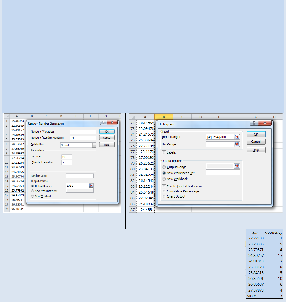
Activity – Random Number Generation and Plotting a Histogram in Microsoft Excel®
The point of this activity is to help you visualize how N,
, and
σ
affect the distribution of data points
within a sample set.
Many of the advanced statistical tools available in Excel® are found in the Analysis Tool Pack. The
Analysis Tool Pack is not included in the default installation of Excel® so you may need to “turn it on” if
you have never used advanced statistical tools in your copy of Excel®. Each version of Excel® has
different steps for activating the Analysis Tool Pack. Activate the help screen on your copy of Excel® and
select Analysis Tool Pack and then follow the instructions for your particular version of Excel®
First we will use Excel’s random number generator. Select Random Number Generation from the Data
Analysis Tool Pack. The Random Number Generation dialog box will open (see Figure 22.7). Fill in the
fields as shown. The random number generator will return a string of numbers with a mean of 25 and a
standard deviation of 1.
Figure 22.7: Random Number Generator
Dialog Box
Figure 22.8: Histogram Dialog Box.
Next select Histogram from the data analysis tool pack. The Histogram dialog box will
open (see Figure 22.8). Fill in the Histogram dialog box as shown and select “OK”. Excel
will generate a data table similar to the one shown to the right. To generate a
histogram Plot the Bin # vs. Frequency as a Column Graph. Your graph should resemble
Figure 22.6. You should notice that the histogram has the beginnings of a bell curve but
the existence of random error is visibly evident. Now repeat this activity with a much
larger N values such as 1000 or 2000. Observe how the shape of the histogram has
changed. Repe
at the exercise again and this time decrease the standard deviation.
What affect does N and
σ
have on the shape of the histogram?
680
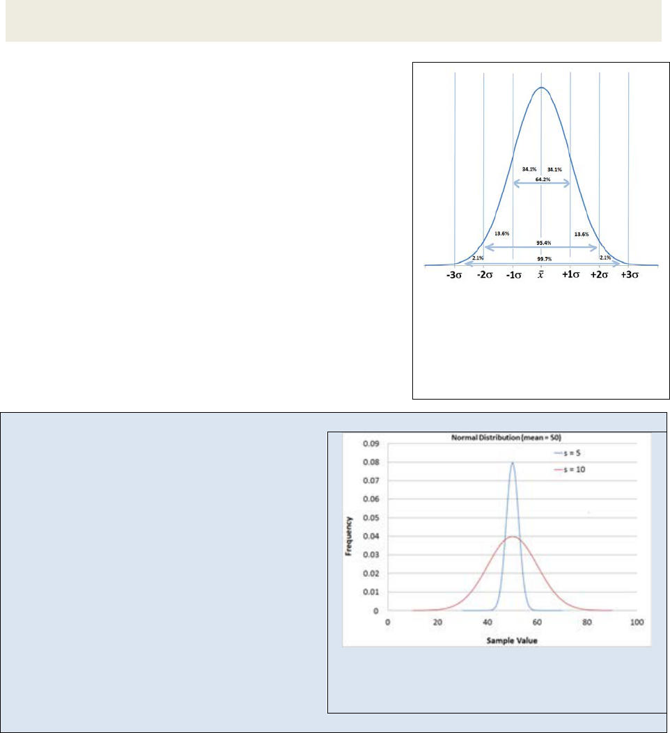
Figure 22.9
: Normal probability
distribution. The ranges indicate the
percentage of all data points as a
function of the distance from the
mean. The x-
axis is in standard
deviations from the mean.
Exercise 22.4: In your own words, explain how changing N and changing σ affects the
histogram generated in the above Activity.
A normal probability function represents the way data is
scattered about a mean when the error in the sampling is
the result of random error. Figure 22.9 shows a normal
probability distribution with the area under the curve
integrated as a function of standard deviation. We see
that 68.2% of all data points fall within a range of ±σ
from the mean, 95.4% of all data points fall within ±2σ of
the mean and by the time we get to ±3σ from the mean
we have incorporated 99.7% of all data points. If we
repeated an analysis 1000 times, we could reasonably
expect that only 3 data points would fall outside the ±3σ
range. Knowing the standard deviation allows us to
predict the likelihood of the next sampled data point
residing within a specified range from the mean.
Example 22.1: The Bell Curve’s shape as a function of the standard deviation
Figure 22.10 shows two different normal
probability functions (npf). Imagine these two npf
curves represent the analysis of a chemical
sample under different experimental conditions.
Each experiment produced a sample mean of 50
however one technique produced a data set with
a standard deviation of 5 while the other data set
had a standard deviation of 10. In the case where
s = 5, nearly 99.7% of all data points fell within
the range of 40 – 60. In the case where s = 10, we
have to expand the range to 20 – 80 in order to
capture 99.7% of all data points. If we could only
afford to repeat the analysis a few times (time =
$) we would have a lot more confidence that our
sample mean is close to the population mean for
Figure 22.10: Two npf curves. The narrow curve
has a standard deviation of 5. The wide curve has a
standard deviation of 10.
the technique where s = 5 than we would for the technique where s = 10.
681
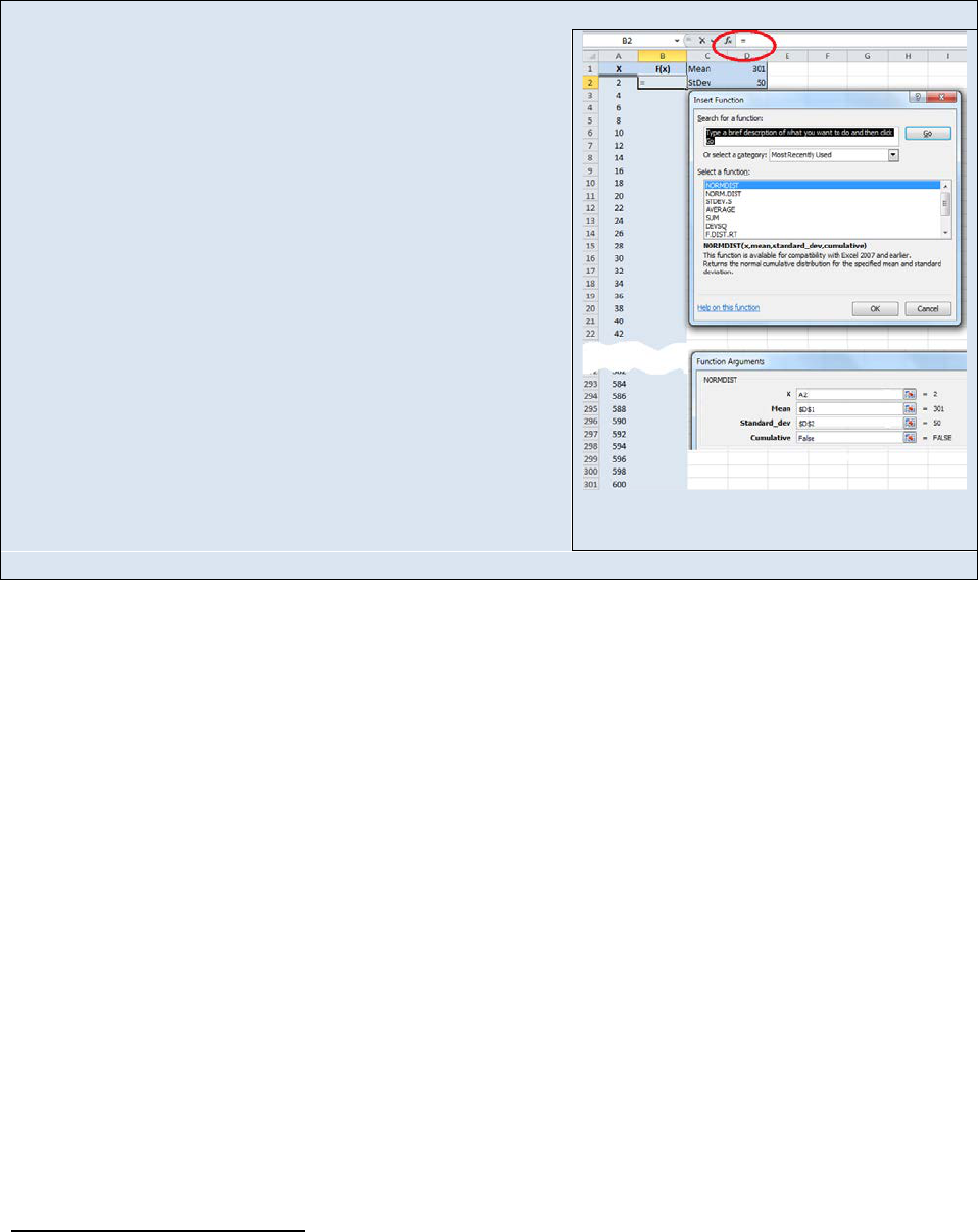
Activity –Plotting a normal distribution function in Excel®
Create the following worksheet in Excel® (See Figure 22.11)
Create a column of numbers from 2 to 600 in intervals of 2
in cells A2
A601. Place a mean value of 301 in cell D1
and your standard deviation of 50 in cell D2. Then select cell
B2 and click the “insert function” link (f
x
) and choose
NORMDIST. The ”Function Arguments” box will open. For
the “x” argument choose cell A2. For the “Mean” argument
box, type $D$1 and for the standard deviation argument
box, type $D$2. The dollar signs in the cell addresses lock
the addresses and prevent them from scrolling. In the
“Cumulative” argument field type the word “FALSE”. The
NORMTDIST function will use Equation 22.
5 to return a
probability value for obtaining a value of “2” in cell B2.
Select cell B2 again and drag and drop it to cell B601. The
“B” column now contains the probability of obtaining the
values listed in the “A” column. Plot an XY scatter plot of
cell
s A2:A601 vs. B2:B601 and insert the graph in your
worksheet. You should see a classic “bell curve”. Now play
with your mean and standard deviation values and observe
Figure 22.11: Example Spreadsheet for
programing a Gaussian Curve.
how the shape of the Gaussian distribution changes as a function of each variable.
Confidence Limits
Earlier we learned how to calculate a standard error. Another common statistical tool for
reporting the uncertainty (precision) of a measurement is the confidence limit (CL). For
example we might report the percent alcohol in a solution as 13% with a 95% CL of ±2%, where
the ±2% represents the CL.
Unless otherwise stated, the reported CL is at the 95% CL and represents the range in which we
are 95% certain the “true” answer lies. The reason the 95% CL is the accepted norm is because
95.4% of all data points in a normal distribution is encompassed by a range of approximately
±2σ. It is reported at 95% instead of 95.4% for purposes of simplicity. However as you will
soon see, it is possible to calculate CL values other than the 95% CL.
We define CL using σ. Recall that σ is the standard deviation of the entire population. When
we do not know σ we use “s” instead and a fudge factor, which we will describe shortly. If we
know the standard deviation for the entire population, then the 95% CL
10
is simply
95% CL = ±2σ Eq. 22.7
and we would report the mean as
10
To be completely accurate, the 95% confidence limit is actually the 95.4% confidence limit because it represents
±2σ from the mean (see Figure 22.5).
682
µ ±2σ
However we seldom know the mean or the standard deviation of an entire population. All
chemical analyses deals with a sampled populations. The CL for a sample is given in Equation
22.8
= ±
Eq. 22.8
and we would report the average as
11
±
were
is the mean of the sample, “s” is the
standard deviation of the sample, N is the number of
data points in the sample and “t” is a “fudge factor”
taken from Table 22.1.
Using Spreadsheets to Determine Confidence Limits
As we have seen, modern spreadsheets such as
Microsoft Excel® are capable of very sophisticated
statistical analysis. The following Activity will walk
you through the steps of calculating the CL for a
sample mean.
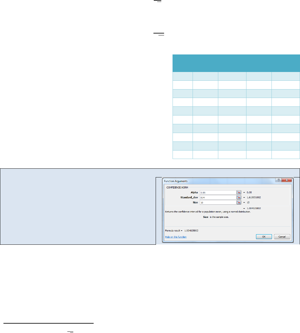
Activity- Using Excel to calculate confidence limits.
Open the spreadsheet Fish that you created in the
previous activities. We are going to use Excel® to
determine the 95% CL of our data set.
Select cell B16 and click on the f
x
button once again.
From the Insert Function dialog box select
CONFIDENCE.NORM. The following dialog box will
appear. To calculate a 95% CL you need to input the
11
Recall that we defined
as the standard error in Equation 22.5.
12
The term (N-1) is the degrees of freedom for the sample set.
Table 22.1: Confidence Limit t-values as a
function of (N-1)
12
N-1
90%
95%
99%
99.5%
2
2.920
4.303
9.925
14.089
3
2.353
3.182
5.841
7.453
4
2.132
2.776
4.604
5.598
5
2.015
2.571
4.032
4.773
6
1.943
2.447
3.707
4.317
7
1.895
2.365
3.500
4.029
8
1.860
2.306
3.355
3.832
9
1.833
2.262
3.205
3.690
10
1.812
2.228
3.169
3.581
683
uncertainty in the Alpha field as 1.00 – CL You need
to input the CL as a decimal (1.00 –
0.95 = 0.05).
Enter the standard deviation (or the address of the
standard deviation) into the “Standard_dev” field. In
the “Size” field enter the value of “N”; the total
number of data points (10) and click “OK”.
At this point, your spreadsheet should resemble the
one shown in Figure 22.12. You can calculate other
CLs by changing the value of alpha.
In this activity we calculated the 95% CL
for the
analysis of mercury in fish. If we were to report the
answer to the hundredth place we would say that
the average concentration of mercury in fish is 5.10
with a 95% CL of ±1.00. The implication of the CL is
that we are 95% certain that the “true” value lies
Figure 22.12: Data for the analysis of mercury in
fish flesh. The data includes the mean, standard
deviation, standard error, 95% C.L. and a plot of
the data showing the S.E. as error bars.
between 4.1 ppb and 6.1 ppb. Or to state this another way, if we repeated the experiment one more
time, we are 95% confident that the next data point will lie within this range.
Exercise 22.5: For the data set used in the above activity, determine the 90% and the 99% CL
Exercise 22.6: For the data set below, determine the mean, standard deviation and 95% CL
3.06
Propagation of Error
Reporting the standard deviation, or the standard error or the CLs for a measured data point is
an acceptable way of portraying the precision of a measurement. But what do you do if you
use two or more measured values in a computation? How do you report the confidence in the
computed value? For example, imagine you determined the density of an object by
independently measuring the mass and the volume. Each of those measurements contains
error. In other words, you have an error associated with both the volume measurement and
the mass measurement and when we divide the mass by the volume to get density we want to
be able to report the composite error of the resulting density. We need to know how to
propagate the standard deviations through various mathematical manipulations. Table 22.2
outlines this process
13
. The standard deviation of a computed result is given as S
R
where R is
the computed result.
Once you have propagated the standard deviation through the mathematical manipulations,
the 95% CL can be approximated as ±2s. Similarly, the 99.7% CL can be approximated as ±3s
however, if you wish to calculate a CL other than the 95% CL or the 99.7% CL you will need to
13
For more on propagation of error see Data Reduction and Error Analysis for the Physical Sciences 3
rd
ed. by Philip
R. Bevington and K. Robinson. McGraw Hill, 2002 or Math for Chemistry 2
nd
ed. By Paul Monk and J. Munro.
Oxford University Press, 2010.
684

determine the degrees of freedom (df) for the calculated value using Equation 22.9 and then
use Equation 22.8 or Microsoft Excel® to find the CL
Table 22.2: R = Computed Result. S
R
= Standard Deviation of Result
Calculation
Example
Standard Deviation of Result (R)
Multiplication/Division
R =
( )
( )
S
R
= R
+
+
+
Addition/Subtraction
R = α − β + γ + δ
S
R
=
+
+
+
Logarithm
R = log(α)
S
R
=
.
Inv. Log
R = inv-log(α)
S
R
= R(2.303S
α
)
Exponents
R = α
x
S
R
= RX
α
,
β
,
γ
and
δ
are experimentally derived data with standard deviations of s
α
, s
β
, s
γ
&
s
δ
respectively.
df =
(
)
(
)
Eq. 22.9
where N
α
, N
β
, N
γ
and N
δ
are the number of replicate data points for the experimentally
derived data sets α, β, γ and δ with standard deviation of s
α
, s
β
, s
γ
& s
δ
respectively.
Example 22.3 – Let us imagine we were determining the volume of an unknown solid by displacement of
water in a graduated cylinder (∆V = V
f
-V
i
). The initial volume was 23.40ml and the final volume was
24.95ml and ∆V = 24.9 – 23.2 = 1.7ml. You might be tempted to conclude that the uncertainty is ±0.1ml.
However if you were to be rigorous in your propagation of error you would recognize there was an
implied ±0.1ml uncertainty in both the initial and final volume readings. Table 22.2 showed us that the
proper way to estimate error when subtracting two numbers is
S
∆V
=
+
=
. = .
Now let us imagine we determined the mass on a digital balance and obtained a value of 3.003 grams. If
you recall what you were taught about significant figures, the implication is that the uncertainty is in the
thousandth place and a reasonable estimate of the standard deviation would be ±0.001g. What is the
uncertainty in the density?
=
=
.
.
= .
If you simply applied the rules for reporting significant figures, you might assume the uncertainty in this
number were ±0.01, however since we have a calculated data point resulting in measurements made
with different precisions, a more rigorous application of propagation of error is required. Take another
look at Table 22.2. The equation for propagation of errors for multiplication and division is
685
S
d
= R
+
= .
.
.
+
.
.
= .
We would want to report our final density as
= .
± .
Exercise 22.7: Assume you measured the mass of 1.0014 grams of potassium oxalate (K
2
C
2
O
4
)
on a digital balance and placed it in a 1 liter volumetric flask with a rated precision of 0.001
liters. Calculate the molarity of the final solution and report the molarity with a 95% CL using
the appropriate propagation of error equation.
Analyzing Data Sets
In addition to reporting the error associated with an individual data set, the analytical chemist
often needs to compare and analyze the variance in data taken under different circumstances.
The different circumstances can be as benign as collecting data on different days or potentially
more significant such as collecting data using different instruments or data collected by
different technicians. For example, imagine you are perfecting a C-18 reverse phase HPLC
method for the purification of a pharmaceutical product. In the final protocols, how important
is it that you purchase your C-18 columns from the same manufacturer each time you replace
the column? Are the changes you see in the data when you change suppliers statistically
significant? We could ask the same question of the solvent. Is it statistically important that we
use the same supplier of solvent every time we run the procedure? We can investigate these
types of questions by using several different statistical tools.
Because of random error anytime you repeat an analysis, you expect to obtain different results.
But are the observed differences within the expected variance of the technique? This is a
fundamental question in an analytical lab. You may have a data point that seems significantly
different than the other replicates in the data set and you would like a statistical basis for
keeping or rejecting that data point. Or you may want to know the effect of a particular
experimental parameter on the overall variance of a method. For instance, when comparing
the means of data taken by two different lab technicians, are the observed differences in the
means statistically significant? Or you may want to compare the results of an analysis using
two different instruments (i.e. two different UV-vis spectrometers) or two different techniques.
Again you will want to answer the question “are the observed differences statistically
significant”. In the next few section, we will introduce tools that you can use to help answer
these types of questions.
686

Identifying Outliers: Q-Tests
Although the International Organization of Standardization (ISO) now
recommends that we use the Grubb’s test for identifying outliers, the Q-test
still remains a very commonly used method and we introduce it here because
you are likely to encounter it in your careers. We will examine the Grubb’s test
in the next section.
Sometimes you obtain a set of replicate data and there is one (or more) data
point that just “seems wrong”. For example, Table 22.3 shows the results for
the N = 10 replicate analysis of caffeine in tea. The data points tend to cluster
around 80 ppm with the exception of Cup #5 which had a lower reading of 72
ppm. The sloppy analyst might be tempted to throw out Cup #5’s data based
solely on intuition; however it is quite possible that 72 ppm falls within the
95% confidence interval for this distribution of points. It is unethical to simply
ignore data that you dislike. You should include all data in a report, even
outliers, and if you decide to reject a point in your final analysis, you must have
a statistical justification for that decision. A Q-test is a statistical tool used to
identify an outlier within a data set
14
. To perform a Q-test you must first
arrange your data in a progressive order (low-to-high or high-to-low) and then
using Equation 22.10, you calculate an experimental Q-
value (Q
exp
). If Q
exp
is greater than the critical Q-value
(Q
crit
) found in Table 22.4 then you are statistically justified
in removing your suspected outlier from further
consideration.
15
You then recalculate the mean, standard
deviation and the 95% CL with the outlier removed from
the calculations.
=
Eq. 22.10
X
q
= suspected outlier
X
n+1
= next nearest data point
w = range (largest – smallest data point in the set)
14
R. B. Dean and W. J. Dixon "Simplified Statistics for Small Numbers of Observations". Anal. Chem., 23 (4), 1951,
636–638 // Rorabacher, D.B. "Statistical Treatment for Rejection of Deviant Values: Critical Values of Dixon Q
Parameter and Related Subrange Ratios at the 95 percent Confidence Level". Anal. Chem., 63 (2), 1991, 139–146 //
Table 22.3
Cup
ppm
Caf
1
78
2
82
3
81
4
77
5
72
6
79
7
82
8
81
9
78
10
83
Avg
79.3
StDev
3.3
95%
C.L.
2.0
Table 22.4: Critical Rejection
Values for Identifying an Outlier:
Q-test
Q
crit
N
90% CL
95% CL
99% CL
3
0.941
0.970
0.994
4
0.765
0.829
0.926
5
0.642
0.710
0.821
6
0.560
0.625
0.740
7
0.507
0.568
0.680
8
0.468
0.526
0.634
9
0.437
0.493
0.598
10
0.412
0.466
0.568
687
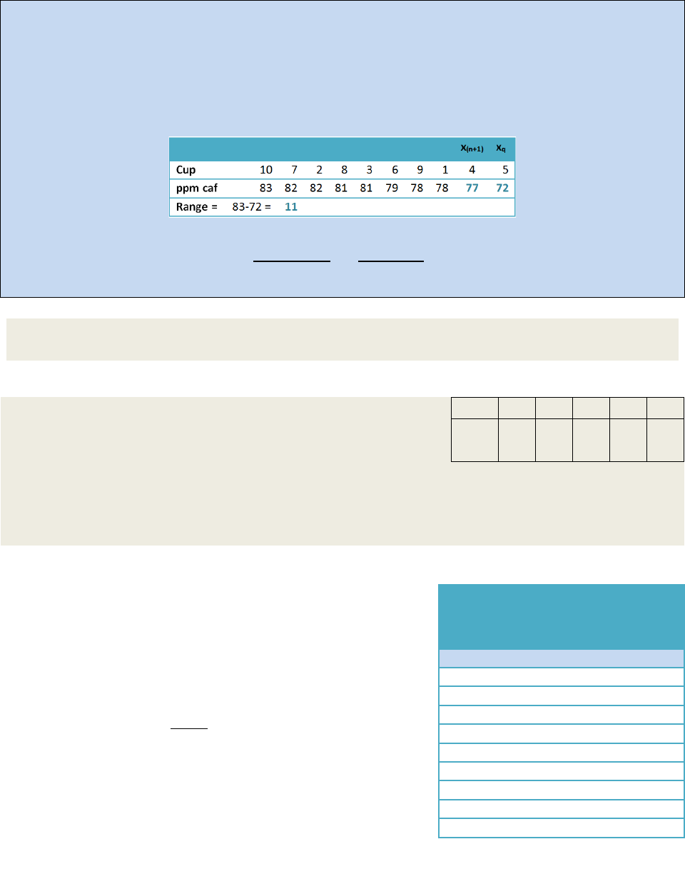
Example 22.4- Perform a Q-test on the data set from Table 22.3 and determine if you can statistically
designate data point #5 as an outlier within a 95% CL If so, recalculate the mean, standard deviation and
the 95% CL
Strategy – Organize the data from highest to lowest data point and use Equation 22.10 to calculate Q
exp
.
Solution – Ordering the data from Table 22.3 from highest to lowest results in
Substitution into Equation 22.10 yields
=
=
|
|
= .
Using the Q
crit
table, we see that Q
crit
=0.466. Since Q
exp
<Q
crit
, you must keep the data point.
Exercise 22.8: Use the data in Table 22.3 and determine what value (in ppm) would cup #5
have to be before Equation 22.10 would identify it as an outlier. Show your work.
Exercise 22.9: Imagine the following set of 5 replicate data
were collected for the analysis of lead in drinking water.
Trial
1
2
3
4
5
ppm
(Pb)
1.3
1.4
1.0
1.3
1.4
(a) Calculate a mean, standard deviation and 95% CL on the data set (you may want to use
a spread sheet).
(b) Perform a Q-test on the data set. How does the performance of a Q-test alter your
answer in part a?
Identifying Outliers: Grubb’s-Tests
The recommended way of identifying outliers is to use the
Grubb’s Test. A Grubb’s test is similar to a Q-test however
G
exp
is based upon the mean and standard deviation of the
distribution instead of the next-nearest neighbor and range
(see Equation 22.11).
=
Eq. 22.11
If G
exp
is greater than the critical G-value (G
crit
) found in
Table 22.5 then you are statistically justified in removing
your suspected outlier from further consideration. You
then recalculate the Mean, Standard Deviation and the 95%
CL with the outlier removed from the calculations.
Table 22.5:
Critical Rejection
Values for Identifying an
Outlier: G-test
G
crit
N
90% C.L.
95% C.L.
99% C.L.
3
1.1.53
1.154
1.155
4
1.463
1.481
1.496
5
1.671
1.715
1.764
6
1.822
1.887
1.973
7
1.938
2.020
2.139
8
2.032
2.127
2.274
9
2.110
2.215
2.387
10
2.176
2.290
2.482
688

Exercise 22.10: Perform a Grubb’s test on the data set found in Exercise 22.9. Report the
mean, standard deviation and the 95% CL based upon the results of your Grubb’s test.
Analyzing Variance: F-Tests
The F-test is named after Ronald Fisher who first developed the test in the 1920’s
16
. The test
allows for the comparison of the variance of two different data sets in order to determine if
there is a statistically significant difference. It is common in a working lab to have data sets that
were obtained under different circumstances. For instance, data may have been collected on
different days, or you may have two different analysts conducting the same measurements.
When the final results vary, you need a way to determine if the difference is statistically
significant. In a manner similar to the Grubb’s test and the Q-test, you perform an F-test by
calculating an experimental F-value (F
exp
) and comparing that to a critical F-value (F
crit
). If
F
exp
>F
crit
then the variance of the two data sets used to calculate F
exp
are statistically different.
F
exp
is determined by the ratio of the sample variances (square of the standard deviations). The
larger variance value goes in the numerator so that F
exp
is always greater than one.
=
Eq. 22.12
In this case, the null hypothesis is that the two variances represent the same population. To
reject (or accept) the null hypothesis, we compare F
exp
to F
crit
. The tables for critical F values
are tabulated as a function of CLs and degrees of freedom for
,
and
. As a result a full set
of F-tables can be extensive. Table
22.6 is an example of critical F-
values at the 95% CL for degrees of
freedom up to 10.
Fortunately we do not need a
complete set of F-tables on hand.
Microsoft Excel
®
can be used to
perform F-tests. Example 22.5
shows an example data set collected
from the HPLC analysis of residual
acrylamide from a batch of
polyacrylamide
17
. In this study two
different analysts performed ten
replicate studies. The results
showed a mean value of 10.1 ppb for analyst #1 and 10.5 ppb for analyst #2 with standard
deviations of 0.9 and 1.5 respectively. The mean values of 10.1 and 10.5 may seem similar
enough with a gross deviation between the two means of only 0.4 but what you really want to
16
R. A. Fisher Statistical Methods, Experimental Design and Scientific Inference. Oxford University Press: New York,
1990, 1991, 1995, 1999.
17
Polyacrylamide is a water absorbent polymer used in diapers. The monomer is a neurotoxin so it is critical that
each batch be tested for residual monomer concentration before it is sent to market.
Table 22.6: 95% C.L. F-Test Critical Values. The degrees of
freedom used to calculate
,
and
represent the column
and row headings respectively
Numerator Degrees of Freedom
Denominator
Deg. Free.
1
2
3
4
5
7
10
1
161.5
199.5
215.71
224.6
230.2
236.8
241.9
2
18.51
19.00
19.164
19.25
19.30
19.35
19.40
3
10.13
9.552
9.2766
9.117
9.014
8.887
8.786
4
7.709
6.944
6.5915
6.388
6.256
6.094
5.964
5
6.608
5.786
5.4095
5.192
5.05
4.876
4.735
7
5.591
4.738
4.3469
4.12
3.972
3.787
3.637
10
4.965
4.103
3.7082
3.478
3.326
3.135
2.978
689
determine is if a gross deviation of 0.4 is within a 95% confidence interval for the standard
deviations of the data sets. Example 22.5 walks you through the performance of an F-test.
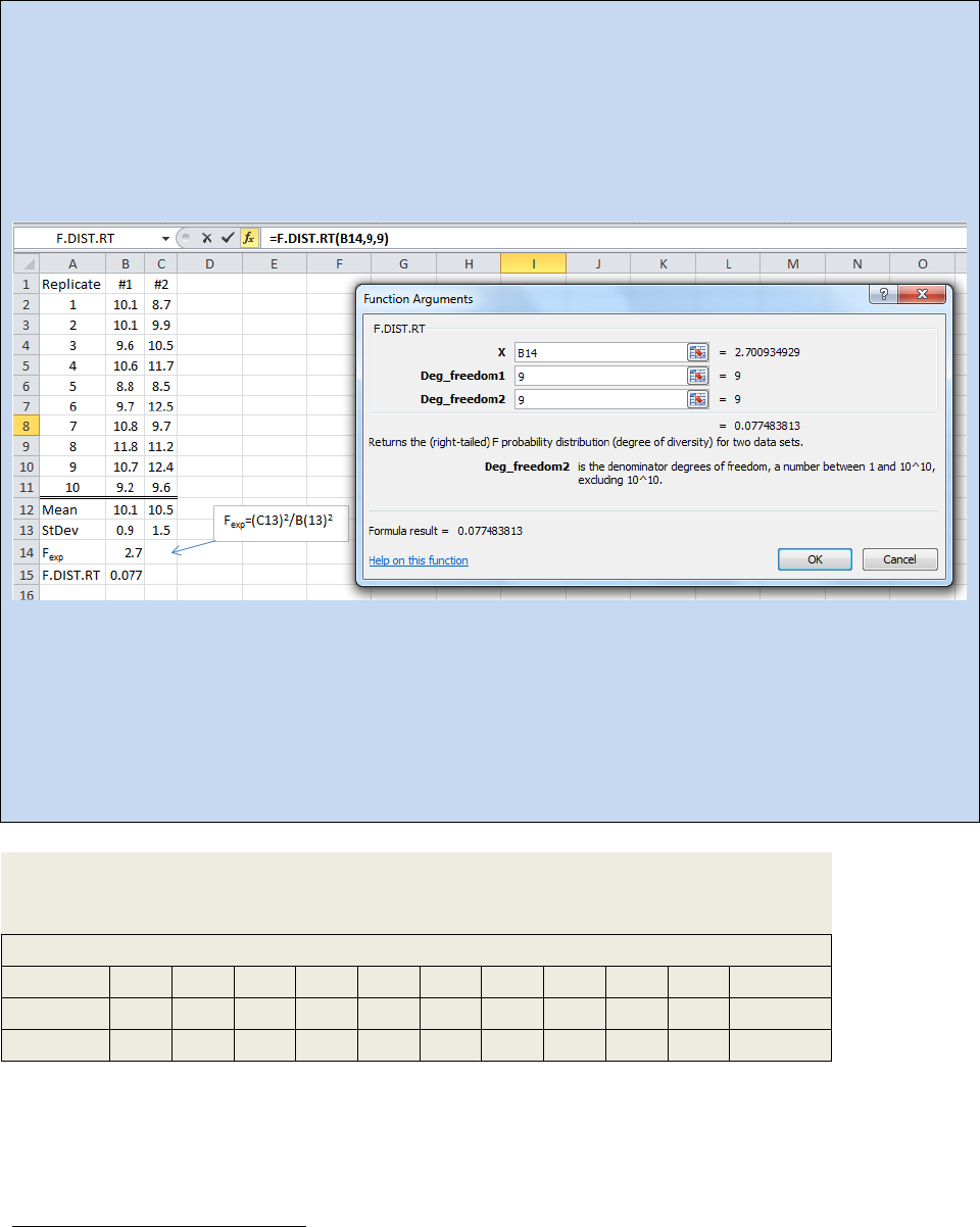
Example 22.5: To perform an F-test using Excel, you need to enter your data as shown in the
spreadsheet below and determine the standard deviation for each data set (for example see cell B13
and C13). Then determine the experimental F-value using Equation 22.12 and put that value into one of
the cells (Here we used B14). Next you need to click on the insert function button (f
x
) and choose
F.DIST.RT. The Function Argument dialog box will open as shown.
______________________________________________________________________________
Spreadsheet 22.1: Right Tailed F-Test comparing the results of two different analysts for the
measurement of residual acrylamide monomer in a batch of polyacrylamide (ppb).
______________________________________________________________________________
Enter your experimentally determined F-value for x and the numerator degrees of freedom
18
for
Deg_fredom1 and the denominator degrees of freedom for Deg_fredom2 and click “OK”.
In the above spreadsheet, the F-test returned a value of 0.077. If we round that to 0.08 then what this
test tells us is the two sets of data can be considered the same if we also accept a CL of 92% (1.00 – 0.08
= 0.92). If we need an 95% CL, we need the F-test to return a value of 0.05 or less.
Exercise 22.11: You have just measured the pH of the water sampled from a local lake.
You have ten replicate measurements with two different pH probes. The data is
presented below. Conduct an F-test on the data set and comment on the results.
pH of Local Lake Water
Replicate
1
2
3
4
5
6
7
8
9
10
Avg. pH
Probe 1
6.74
6.49
6.71
6.62
6.76
6.67
6.99
6.68
6.96
6.52
6.71
Probe 2
6.93
6.83
6.90
6.79
6.88
6.64
7.10
7.18
7.04
6.97
6.93
18
See Equation 22.4 for a review of degrees of freedom.
690

Exercise 22.12: In 2006, the Arundel County Maryland Department of Health tested local wells
for elevated levels of arsenic. They found that 35 out of 71 wells showed elevated levels.
Atomic Absorption Spectroscopy is a very convenient way to measure arsenic in water. Imagine
you are a lab manager and you have given identical arsenic samples to two different
technicians. Conduct an F-test on the two sets of data and comment on the results.
Replicate
1
2
3
4
5
6
7
8
9
10
Avg. ppb (As)
Tech. 1
0.304
0.306
0.301
0.320
0.324
0.276
0.302
0.329
0.304
0.297
0.306
Tech. 2
0.331
0.285
0.317
0.298
0.346
0.239
0.307
0.258
0.308
0.326
0.302
ANOVA: A two dimensional F-test
ANOVA is an acronym for ANalysis Of VAriance. It is very similar in concept to an F-test and in
fact we actually calculate an F-value in the analysis. For example, in Example 22.5 above, we
imagined a scenario where two different analysts performed the same test on the same batch
of polyacrylamide. Let us imagine next that we sent that same batch of polyacrylamide out to
five different labs and upon receiving the data, we wished to statistically compare the results.
We could conduct an F-test on each possible pairing of labs but that would be tedious and the
results hard to interpret. A more sophisticated approach would be to compare the average
variance that occurs as a result of changing labs to the average variance that occurs as a result
of performing replicate samplings. Spreadsheet 22.2 shows the raw data along with an ANOVA
analysis with inputs conducted by hand for the purposes of demonstration. Fortunately for us,
Excel® will do an ANOVA automatically and you will not need to program each cell manually
(see spreadsheet 22.3).
There are a total of 50 replicate data points when you combine the data from all five labs. The
average result of all 50 points is called the Grand Mean. In this case we obtained a value of
10.31 ppb. For each data point the deviation from the grand mean was calculated (columns:
D,G,J,M,P). This value is termed the mean corrected value (d
ij
). Next we squared the mean
corrected values (d
ij
2
) to generate positive numbers (columns: E,H,K,N,Q). Next we summed all
of the d
ij
2
values (SS
c
) and then divided SS
c
by the degrees of freedom
19
to yield
c
. Compare
the derivation of
c
to the derivation of a standard deviation (Equation 22.4). The value
c
is
essentially the grand standard deviation of replicates between labs. Similarly we also
calculated a
r
value.
r
can be thought of as the grand standard deviation of labs between
replicates. The F-value is then determined by dividing
c
by
r.
How one uses an F-value is
demonstrated in the next Activity.
19
See Equation 22.4 for a review of degrees of freedom.
691
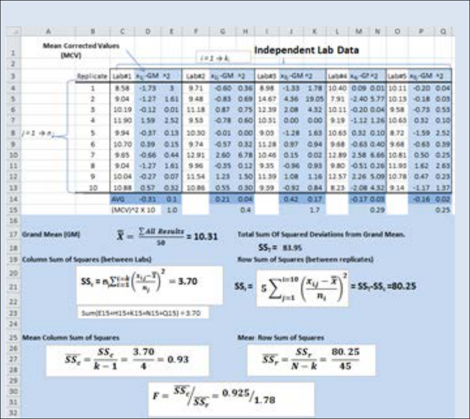
Spreadsheet 22.2:-Analysis residual monomer (ppb) found in a batch of polyacrylamide conducted at 5
different independent labs; An ANOVA between 5 independent labs.
692
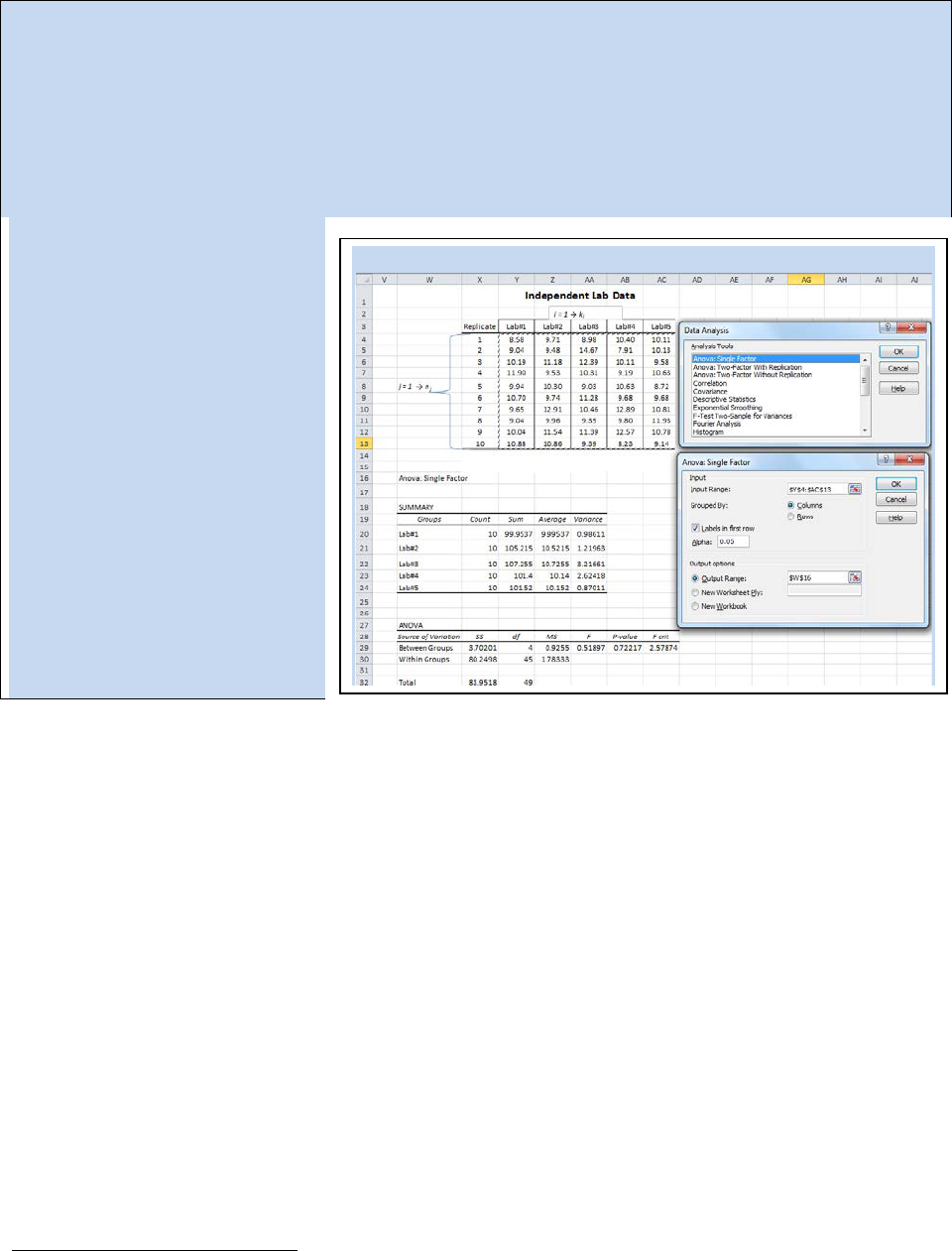
Activity - Letting Excel Perform ANOVA
Using the same data we examined in Spreadsheet 22.2, we will perform an ANOVA using the ANOVA
statistics function in Excel. From the data analysis tool pack, select “ANOVA: Single Factor”. The ANOVA
Single Factor dialog box will open (see Spreadsheet 22.3). The input range is the total 50 data points
obtained between all five labs. In this example, we have the independent labs arranged in columns so
make sure the “Grouped By Columns” radial button is selected. Notice that we have also selected the
“Labels in first row” check box. The default value for α is 0.05 which will calculate a 95% confidence
interval for your ANOVA. You have several options for the output. If you choose to keep your ANOVA
output with your raw data, then
you have to tell Excel where you
want the data table to start. In
this case we began our data table
at cell W16.
The ANOVA table in Spreadsheet
22.3 has a calculated F-value of
0.51897 (the same value we
calculated by hand). The p-value
shown is called the value of
probability. Since we selected an
alpha value of 0.05, we want our
p-value to be above 0.05 in order
for the null hypothesis to hold. In
other words, this ANOVA study did
not find any statistically significant
variance between the five labs.
22.5 – Linear Regression Analysis
The preceding section provides tools useful to the experimenter when working with repetitive
data – that is, measurements that are expected to have essentially the same value every time.
When conducting instrumental analysis, however, it is often the case that we do not know in
advance the actual magnitude of the measurement, but only an estimate of a range in which
the measurement might fall. In such cases, we must prepare and measure standard samples
20
that fall in the expected range in order to calibrate the instrumental response for known
concentrations. The fundamental signal that is obtained from an instrument is either a voltage
or a current, neither of which directly gives us useful information about our sample. In practice
we use standard calibration curves to relate that fundamental signal to one that is more
meaningful, such as pH or absorbance. We then plot that signal as a function of known
concentrations to yield a calibration curve so that the signal from an unknown sample can be
used to determine the analyte concentration. The basic statistical tools outlined above must be
further developed for application to measurements made using a calibration curve.
For an instrument response that is linear with analyte concentration, we would expect to
obtain a series of data points that fall on a straight line as the concentration is varied. However,
20
Recall that a standard sample is one in which the concentration of analyte is known.
Spreadsheet 22.3: A Single Factor ANOVA in Excel.
693
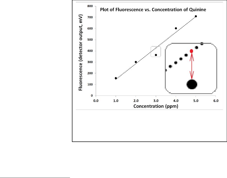
Figure 22.13: Demonstration of the y-residuals. The region around
the third point is expanded in the inset. The red dot represents
y
i,calc
and the large black point represents y
i,act
. The difference
between the two points is (y
i,act
– y
i,calc
) for i=3.
we also expect there to be error in the measured values so the points will have some degree of
variance from the anticipated straight line. If we were to graph those values on paper, we
could use a straightedge to estimate a best fit line for the points. In the modern electronic age,
however, it is more common (and more accurate) to use a method called regression analysis to
discover the best linear approximation from the measured points.
Much of what we need for our analyses can be obtained quickly and easily from Excel™ or
another spreadsheet software package. Using the linest function
21
in Excel™, we can obtain the
slope and intercept for the regression, as well as the standard deviations associated with those
values. Further, we can extract the coefficient of determination, R
2
, also known as the ‘R-
squared’ value and the standard error for the y-estimate (essentially the standard deviation for
the regression), s
y
. The R
2
has a value between zero and 1, and is often referred to as the
“goodness of fit” or a “correlation coefficient”. An R
2
value of 1 indicates a perfect fit between
the actual y-values and those calculated using the linear equation. The farther the R
2
value
deviates from 1, the greater the deviations between the actual and calculated y-values. The s
y
value is used in calculating the standard deviation of results for measurements of unknown
samples obtained using the calibration curve.
It is helpful to understand
how the software goes
about calculating an
equation for the linear
regression. To find a best fit
line (Eq. 22.13), the
software is programmed to
minimize the sum of the
squared differences
(sometimes called residuals)
between the actual y-values
and those calculated by the
linear equation for each x-y
pair. Figure 22.13 provides
a visual depiction of what
we mean by these residuals.
The residuals are squared to
eliminate any negative
values and then the slope of
the line is adjusted until the
sum of the residuals reaches a minimum value. If we call the summed residual values value SS
y-
y
, the software seeks to minimize it in the form of Eq. 22.14.
,
=
+ Eq. 22.13
21
You can accomplish the same thing using the linest function in the function dialog box.
694

=
(
,
,
)
Eq. 22.14
SS
y-y
= sum of the squared residuals
,
= actual (measured) value for y in a given (i) of an x-y pair
,
= y-value calculated from the linear equation Eq. 22.13
Most of what we need for sample analysis can be obtained fairly directly through Excel (see the
Activity on the following page and Example 22.6), but in order to accomplish full statistical
analysis, we need to define one additional quantity, S
x-x
, given in Eq. 22.15. With the
information obtained from the Excel linest function and S
x-x
, we will be able to calculate a
standard deviation for any y-value calculated for a sample of unknown concentration using the
linear regression of the calibration plot (Eq. 22.16).
=
(
)
Eq. 22.15
= value for x in a given (i) of an x-y pair
= the mean of all of the x-values
=
(
)
(
)
+
+
Eq. 22.16
= standard deviation of a calculated y-value for an unknown sample
= standard error in the y-estimate (from Excel linest function)
= slope of the regression line (from Excel linest function)
= mean of all y-values for N
S
replicates of the unknown sample
= mean of all y-values for N
C
samples used in the calibration
= number of samples used in the calibration
= number of replicates of the unknown sample
695
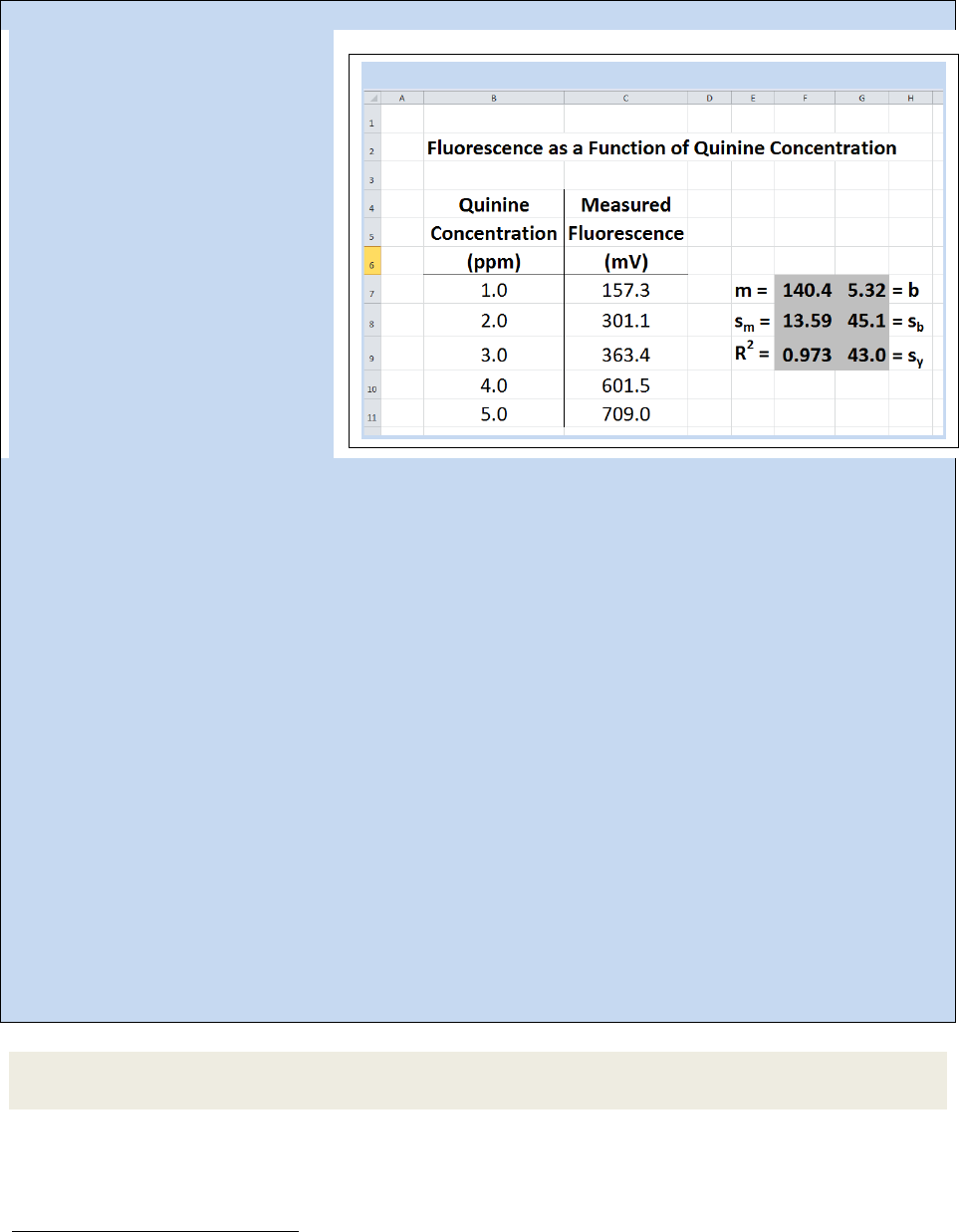
Activity - Letting Excel Perform LINEST to give linear regression data
Set up a calibration data set as
given in Spreadsheet 22.4. To have
Excel calculate the pertinent
analysis data from the calibration
information, we use the linest
function in the following
procedure:
1. Highlight an area encompassing
two columns and three rows
22
(the
highlighted area in Spreadsheet
22.4 is in columns F and G, rows 7-
9).
2. With that area still highlighted,
start typing the function = linest(
3. After the open parentheses,
highlight all the y-values in the
calibration data, then enter a comma.
4. Next, highlight all the x-values in the calibration data, then enter a comma.
5. For the next parameter, you need to make a choice.
a. If you expect that the calibration data should pass through zero (intercept of zero), then enter a zero
followed by a comma.
b. If you want the function to calculate an intercept value, enter a 1, followed by a comma.
6. Now enter a 1, telling Excel to calculate stats beyond just the slope and intercept, close the
parentheses but do not simply press Enter.
7. To complete the calculation, press Ctrl + Shift + Enter (while holding down the Ctrl key, press the Shift
key, and while still holding down both of those, press the Enter key).
In the example given in Spreadsheet 22.4, the completed function looked like this, wherein we allowed
linest to calculate an intercept value:
=LINEST(C7:C11,B7:B11,1,1)
The information that Excel yields from the linest function includes the slope (m, in Cell F-7), the intercept
(b, G-7), the standard deviation in the slope (s
m
, F-8), the standard deviation in the intercept (s
b
, G-8),
the coefficient of determination (R
2
, F-9), and the standard deviation in the y-estimate (s
y
, G-9).
Note that if you need to edit your linest function, you will need to highlight the full 2x3 block again,
make your edits, then press Ctrl + Shift + Enter.
Exercise 22.13: Use Eq. 22.14 to calculate SS
y-y
for the example given in the preceding Activity
(Spreadsheet 22.4).
22
Actually, Excel will provide additional statistics, if we highlight an area that is 2 columns by 5 rows, but the
additional two rows of statistics are not generally as useful as the first 3.
Spreadsheet 22.4: The LINEST function in Excel
696

Exercise 22.14: Repeat Exercise 22.13, but use a slope that is 1% lower and an intercept 1%
higher than that seen in Spreadsheet 22.4. Compare the SS
y-y
you get with that found in 22.13.
Is the result as expected? Explain.
Example 22.6- Following thee calibration represented in Spreadsheet 22.4, three replicates of a quinine
sample of unknown concentration were prepared and the fluorescence measured, yielding the values
406.6, 414.6 and 408.2. Calculate the quinine concentration in the sample and the standard deviation in
the calculated value.
Strategy – Use Eq. 22.13 and the linest data in Spreadsheet 22.4 to calculate the quinine concentration.
Then use Eq. 22.16 to calculate the standard deviation in the calculation.
Solution – The average measured value (
) for the unknown sample is 409.8, so we can calculate the
concentration as
= +
. = . + .
x = 2.8813 = 2.9 ppm
For Eq. 22.16, we will use the following values
s
y
= 43.0 m = 140.4 S
x-x
= 10
= 409.8
= 426.5
N
C
= 5 N
S
= 3
=
(
)
(
)
+
+
=
.
.
(. .)
.
()
+
+
= 0.224 = 0.22 ppm
Exercise 22.15: The following data were obtained for a set of calibration solutions of p-
nitroaniline, measured by absorbance in UV-Visible spectrophotometry.
Concentration (ppm) Absorbance (AU)
19.5 0.980
9.74 0.440
4.87 0.255
0.974 0.101
A p-nitroaniline solution of unknown concentration exhibited an average absorbance of 0.181
for 5 replicate samples. Assuming the intercept is zero for the calibration, calculate the
concentration of the unknown solution and the standard deviation in the calculation.
Exercise 22.16: Repeat Exercise 22.15, but do not assume the intercept is zero for the
calibration. Which set of results do you feel are more accurate? Explain. What additional
information would you need in order to make a more definitive judgment?
697
Exercise 22.17: The following data were obtained for the calibration of an FAA instrument in
the measurement of calcium:
Concentration of Ca (ppm) Absorbance (AU)
0.100 0.010
0.250 0.024
0.500 0.069
1.000 0.093
2.500 0.225
5.000 0.427
7.500 0.628
10.00 0.804
A urine sample was treated to remove interferences, resulting in a dilution factor of 5:2 of the
original urine. The mean absorbance of three replicates of the diluted urine was found to be
0.325. Assuming the intercept is zero for the calibration, calculate the concentration of the
unknown solution and the standard deviation in the calculation.
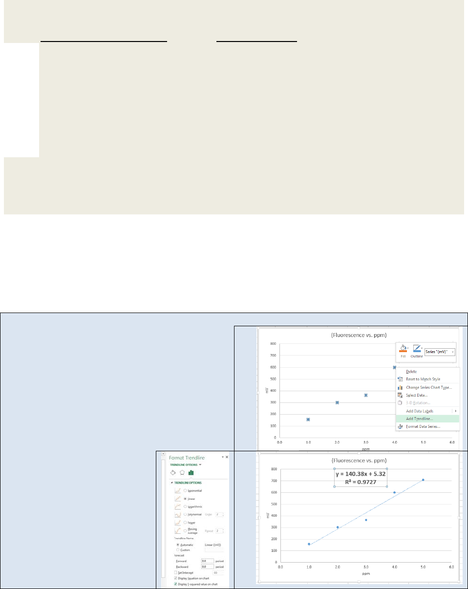
If you don’t need a full statistical analysis of your calibration curve and simply want the y = mx +
b equation and the R
2
value, Excel™ also offers a feature called “add trendline”. The add
trendline feature is accessed by right clicking on the X-Y scatter plot of the calibration data. The
next activity demonstrates the add trendline feature.
Activity – Using Excel™ to add a trend line to a data set.
Using the same data set from our previous activity,
create an X-Y scatter plot as shown here. Highlight
the X-
Y points in the scatter plot and “right click”.
If using an Apple operating system, hold down the
Apple key and click. A dialog box open. Select Add
Trendline. The Format Trendline dialog box will
open (see below).
If you expect your instrument
response to be linear, then select the linear radial
button. Then select Display Equation on Chart
and Display R-squared value on
chart. Hit return. Your graph
should now resemble the one
seen here on the bottom right.
698

22.6 – LOD, LOQ, and LDR
As noted above, we must expect the presence of random error (noise) in every measurement.
Sometimes that noise is clearly visible, but other times it is not obvious. This realization make it
necessary to contemplate the question “At what point can I trust that my measurement is real,
and not just noise?”. Fortunately, statistically sound tools have been developed to help us
make that judgment.
The limit of detection (LOD) is the lowest value measurable above the background noise. At
the LOD, we can be confident that we are measuring some analyte, but we cannot be confident
about the actual amount. The limit of quantitation (LOQ) is the minimum value at which we
can be confident in the quantitative value of the measurement. The IUPAC
23
has demonstrated
the following for any given analytical method:
=
+
Eq. 22.17
LOD
y
= limit of detection of the measurement (y-value)
= mean y-values of a set of blank or baseline measurements
s
blnk
= standard deviation of a set of blank or baseline measurements
k
D
= multiplicative factor. k
D
= 3 at the 99.9% confidence level
=
+
Eq. 22.18
LOQ
y
= limit of quantitation of the measurement (y-value)
and s
blnk
are as above
k
Q
= multiplicative factor. k
Q
= 10 for 10% RSD and k
Q
= 20 for 5% RSD
Note that Equations 22.17 and 22.18 will be relevant for any type of measurement, even if a
calibration plot is not used, as long as we can get a reasonable estimate of the mean blank
signal and its standard deviation.
In many cases involving calibration plots, it is more desirable to think about limits of detection
and quantitation in terms of actual concentrations (the x-value) rather than the measured
quantity (the y-value). Since we know the relationship between x and y for a linear relationship
(y=mx+b), we can derive expressions that give us LOD and LOQ in terms of concentration. Note
that in most instrumental methods, the instrument will be set to a measurement of zero using a
blank solution, so we can assume that in the absence of significant drift, the intercept (b) is
equal to the average blank measurement,
, or
= +
Eq. 22.19
23
Long, GL and Winefordner, JD, “Limit of Detection: A Closer Look at the IUPAC Definition”, Anal. Chem., 55, 1983,
712-724.
699

The “y” in an LOD (or LOQ) calculation is the LOD
y
(or LOQ
y
) from Equation 22.17 (or 22.18), and
the “x” would be the LOD
x
(or LOQ
x
), which is the limit of detection in terms of concentration:
=
+
Eq. 22.20
If we combine Eq. 22.17 and 22.20 (or 22.18 and the LOQ equivalent of 22.20), we can find our
equations for limits of detection and quantitation in terms of concentration (Equations 22.21
and 22.22):
=
Eq. 22.21
LOD
x
= limit of detection of the concentration
s
b
= standard deviation of a set of blank or baseline measurements
k
D
= multiplicative factor. k
D
= 3 at the 99.9% confidence level
=
Eq. 22.22
LOQ
x
= limit of detection of the concentration
s
b
= standard deviation of a set of blank or baseline measurements
k
Q
= multiplicative factor. k
Q
= 10 for 10% RSD and k
Q
= 20 for 5% RSD
Exercise 22.18: Demonstrate that Equations 22.21 and 22.22 can be derived from Equations
22.17 and 22.18, respectively.
Exercise 22.19: Demonstrate that the units of LOD
x
(and thus LOQ
x
) are concentration units.
Assume concentration is in units of molarity and the measurements are made in milliamps from
an arbitrary detector.
Exercise 22.20: In the experiment represented in Exercise 22.17, eight blank measurements
were made: 0.001, 0.000, 0.000, 0.001, 0.002, -0.001, 0.000, -0.001 AU. Calculate the LOD
y
,
LOQ
y
, LOD
x
, and LOQ
x
.
Exercise 22.21: Consider your results from Exercise 22.19 and the data presented in Exercise
22.17. If you were presenting this data for publication, would you need to redo the calculations
you did in Ex. 22.17? Explain.
It is often the case that we do not have available multiple blank measurements for a method
involving a calibration plot. In such a case, two alternatives have been proffered. If, in doing
the linear regression, an intercept is calculated, then we can substitute s
b
(standard deviation of
the intercept) for s
blnk
in the equations presented above. If we set the intercept to zero in the
linear regression, we can use the s
y
(standard deviation of the y-estimate) in place of s
blnk
. In
both cases, we must expect that our estimates for LOD and LOQ will be higher than they would
have been using the formal approach, but it is better to err on the side of caution.
Exercise 22.22: Estimate LOD
x
and LOQ
x
for the data given in Spreadsheet 22.4.
700
