
Pike Li & Shane Heschel
COLORADO COLLEGE
2024
OBE - EXCEL GUIDE TO
HYPOTHSIS TESTING AND
STATISTICAL ANALYSIS IN
ECOLOGY
1
Table of Contents
Definitions ............................................................................................................................ 2
1.1 Keywords for research design .................................................................................................2
1.2 Keywords for statistical analyses .............................................................................................2
1.3 Key symbols ............................................................................................................................3
Descriptive statistics and simple graphs in Excel .................................................................... 4
2.1 Measures of Central Tendency: Mean, Median, and Mode .....................................................4
Mean: ................................................................................................................................................................... 4
Median: ................................................................................................................................................................ 4
Mode: ................................................................................................................................................................... 5
2.2 Measures of Dispersion and Variability: Variance, Standard Deviation and Standard Error .5
Variance: ............................................................................................................................................................. 5
Standard Deviation: ........................................................................................................................................... 6
Standard Error: .................................................................................................................................................. 6
2.3 Interpret Standard Error in barplot .......................................................................................6
Real Statistics: testing of common assumptions in statistics .................................................... 7
3.1 Tool Installation ......................................................................................................................7
3.2 Shapiro – Wilk test of normality .............................................................................................8
3.3 Homogeneity of variances........................................................................................................9
Data Analysis: common statistical tests in Excel................................................................... 10
4.1 Tool Installation .................................................................................................................... 10
4.2 T-test: Testing differences between two means ...................................................................... 11
Unpaired two-sample t-test: compare two means of independent samples ................................................ 11
Paired two-sample t-test: compare two means of paired samples ............................................................... 12
4.3 Linear Regression ................................................................................................................. 13
Real Statistics: non parametric tests ..................................................................................... 15
5.1 Wilcoxon Rank-Sum test ....................................................................................................... 15
5.2 Kruskal-Wallis test ................................................................................................................ 16
Real Statistics: ANOVA and Post-hoc analysis ..................................................................... 17
6.1 ANOVA ................................................................................................................................. 17
One-way ANOVA ............................................................................................................................................. 17
Two-way ANOVA ............................................................................................................................................. 18
6.2 Post-hoc analysis for One-way ANOVA ................................................................................ 20
6.3 Post-hoc analysis for Kruskal-Wallis ..................................................................................... 21
6.4 Additional helpful tests in Real Statistics ............................................................................... 21
Note: “Real Statistics” is an Excel add-on for additional analysis.

2
Part 1
Definitions
Below are some keywords that are important for statistical analyses in ecology and will
frequently appear throughout the document:
1.1 Keywords for research design
1. Dependent variable: response variable or something you measured.
2. Independent variable: variables that might predict your response or dependent variable.
3. Continuous variable: values on numerical scales (e.g., percentage cover, beak length, etc.).
4. Categorical variable: values belong to categories (e.g., presence/absence).
5. Null hypothesis: usually denoted as H
0
, assumes the relationship between two variables does not
exist and any observed pattern is likely due to chance alone.
6. Alternative hypothesis: usually denoted as H
a
, assumes the relationship between two variables
exists and any observed pattern is likely due to the association between two variables.
1.2 Keywords for statistical analyses
1. Normal distribution: the continuous variable of interest has a bell-shaped curve distribution. A
normality test examines whether the data follow a normal distribution.
2. Homogeneity of variance: each group in the categorical variable has approximately equal
variance.
3. Parametric test: statistical tests that assume the data to come from a normal distribution (often
the assumption) and estimate key parameters of that distribution (e.g., mean).
4. Non-parametric test: tests that do not require the data to come from a specific distribution (e.g.,
normal distribution).
5. Post-hoc test: used when there is a significant difference (p 0.05) in an ANOVA with three or
more groups. Post-hoc tests are used to determine which pair-wise comparisons are determining
the significant difference among groups.
6. P-value: the probability of how likely the data pattern you observed is the result of random
chance. A high P-value indicates patterns in your data are likely from random chance, and vice
versa. A general threshold is at 0.05, a P-value less then 0.05 is considered to be statistically
significant. In the context of ecology, if p = 0.05, then there is only a 5% probability that the
3
pattern in your data is attributable to chance, and 95% probability that the pattern has a biological
explanation. We generally accept the null hypothesis if p 0.05, and fail to reject the null
hypothesis if p 0.05. However, with appropriate power, a p-value of 0.10 or less can be
considered marginally significant.
1.3 Key symbols
Note: symbols will be helpful when interpreting the null and alternative hypothesis in each
statistical test.
1.
2.
3.
4.
5.
6.
7.
corrected sum of squares
8.
9.
10. H
0
= null hypothesis
11. H
a
= alternative hypothesis
12.
13.
14.

4
Part 2
Descriptive statistics and simple graphs in Excel
2.1 Measures of Central Tendency: Mean, Median, and Mode
Mean, median and mode are common methods to describe the center of a distribution.
Mean:
Note: a sample is a subset from a population. Often in ecology, we can’t measure our variables
of interests for the entire population (e.g., the entire ponderosa pine forest in a location), what we
can do instead is to measure a subset of it (e.g., take measurements on 30 trees), so we are often
estimating the distribution of a larger population of values.
Calculate means in Excel:
1. “=AVERAGE()”. For example, “=AVERAGE($C$3:$C$12)” would give you the
average of the numbers in column C and rows 3 through 12. You can manually enter
the data range, or you can select the data by clicking and dragging.
Median:
The middle value of an ordered list of observations (the value in which 50% of the data in the
dataset is less and 50% is more).
Unlike mean, median (M) is more resistant toward outliers in the sample, extreme outliers in the
sample can significantly reduce or increase sample mean.
To manually calculate the median of a sample, first order the value from the smallest to
largest (vice versa also works). Add the depth of each value, in terms of its position from
the nearest extreme end.
Value
1
5
6
14
15
18
20
21
Depth
1
2
3
4
4
3
2
1

5
The median is the value that has the depth of d. When d is not an integer, take the average
of two values that have the depth closest to D. In the example above, d = 4.5, so median
is (14+15)/2 = 14.5
Calculate median in Excel:
1. “=MEDIAN()”. For example, “=MEDIAN($C$3:$C$12)” would give you the
median of the numbers in column C and rows 3 through 12. You can manually enter
the data range, or you can select the data by clicking and dragging.
Mode:
Most frequent occurring values in a population/sample.
Calculate means in Excel:
1. “=MODE()”. For example, “=MODE($C$3:$C$12)” would give you the mode of
the numbers in column C and rows 3 through 12. You can manually enter the data
range, or you can select the data by clicking and dragging.
2.2 Measures of Dispersion and Variability: Variance, Standard Deviation and
Standard Error
Variance:
Variance is a measurement of the dispersion in your data. Sometimes you might have data
groups that have similar means but have different degree of spread or variance. Essentially,
variance sums up each data point’s deviation from the mean.
/ corrected sum of squares
1
1
If you wonder why square is necessary, it’s because without it, the result could be zero, which tells us nothing about data’s dispersion.

6
Calculate sample variance in Excel:
1. “=VAR.S()”. For example, “=VAR.S($C$3:$C$12)” would give you the sample
variance of the numbers in column C and rows 3 through 12. You can manually
enter the data range, or you can select the data by clicking and dragging.
Standard Deviation:
Standard deviation (SD) is the positive square root of the variance.
Calculate standard deviation in Excel:
1. To calculate sample SD, “=STDEV(cells) or STDEV.S(cells)”
Standard Error:
Standard error (SE) is an estimate of the variance of the sample mean adjusted for sample size. It
is calculated by dividing the standard deviation with the square root of the sample size.
Calculate standard error in Excel:
1. To calculate SE, “=STDEV(cells)/SQRT(sample size)”; this equation implies that
the larger the sample size, the smaller the SE (less variation around the mean).
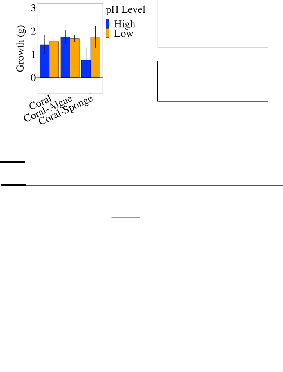
2.3 Interpret Standard Error in barplot
A barplot is a way to summarize your data; a common way researchers use a barplot is to
represent the mean of each group on the y-axis and show the standard error to display the
variation in different groups. You can use SEs to get a sense for whether groups in your dataset
are statistically different from one another:
▪ If the two means are similar and there is overlap in SE→ the difference you see is
likely not statistically significant.
▪ If the two means are far apart and there is no overlap in SE→ any difference you
see is likely statistically significant.
7
Part 3
Real Statistics: testing of common assumptions in statistics
3.1 Tool Installation
To install the “Real Statistics” add-in, click here to download it for your appropriate system. The
file you download should be called “XRealStatsX.xlam”. Do not try to open this file or remove
it even after you added it to your Excel add-on. To connect it to your Excel, either follow the
“Real Statistics Installation” section in the same link or follow the instructions below.
• For Windows:
1. In Excel, go to File → Options → Add-ins.
2. Select “Analysis Tool Pak” from the list. Click “Go”.
3. A new small window will pop up. Check the “Xrealstats” or “Xrealstatsx” option
and click “Ok”.
4. You should now see a “Xrealstas” option under “Data” or “Tools”.
5. If step 3 doesn’t work, click “Browse’ and manually select the
“XRealStatsX.xlam” file on your computer.
• For Mac:
1. In Excel, go to Tools → Excel Add-ins…
2. Select “Analysis Tool Pak” from the list. Click “Go”.
3. A new small window will pop up. Check the “Xrealstats” or “Xrealstatsx” option
and click “ok”.
4. You should now see a “Xrealstas” option under “Data” or “Tools”.
Growth response of coral (mean SE)
expose to different organisms under
ambient and elevated pH. Based on the
information above, the coral growth in
coral-sponge group might be statistically
significant under different pH levels.
Creating graphs like this is possible in
Excel, you can do it by only including the
average of each group in the data range
and manually adding the error bar with
the SE that you calculated.
8
5. If step 3 doesn’t work, click “Browse’ and manually select the
“XRealStatsX.xlam” file on your computer.
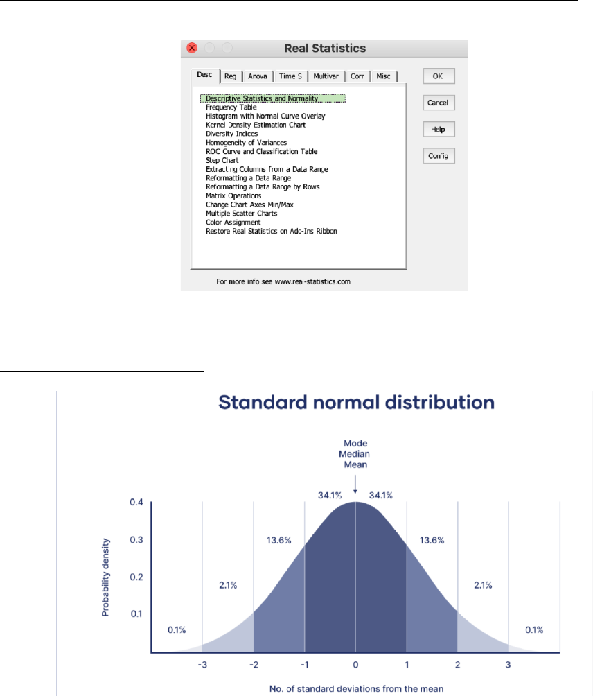
You can open the Real Statistics add-on using Ctrl-m or click the icon under Add-ins.
A window like this will appear:
3.2 Shapiro – Wilk test of normality
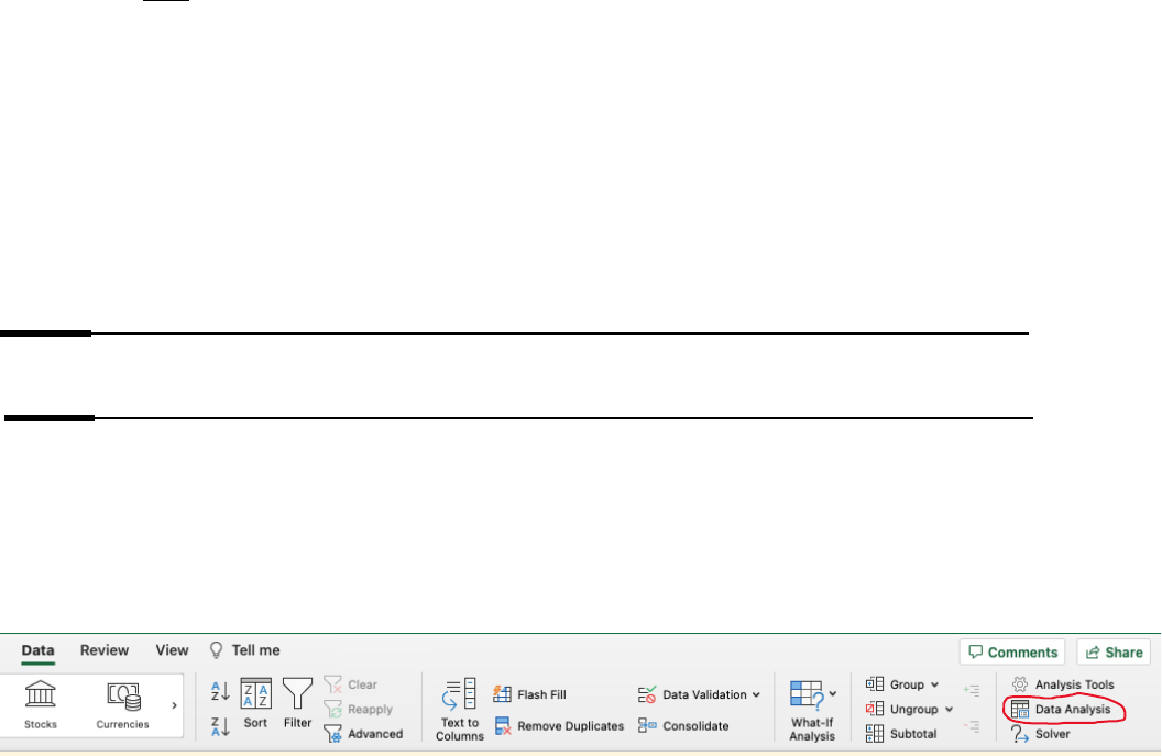
The distribution of many continuous variable in ecology will have a bell-shaped curve or a
normal (Gaussian) distribution.
This is what a bell-shaped curve looks like, with the mean in the middle with highest probability and spread out in
both direction with 1 unit of standard deviation at a time with decreasing probability as the value is deviating from
the mean. In reality, the x-axis would not be centered at zero, it would ideally be centered at the sample/population
mean.

9
Shapiro – Wilk test of normality
Many parametric tests require the continuous variable to be normally distributed to maximize the
test’s accuracy. By performing a Shapiro – Wilk test, we can determine if our data come from a
normal distribution. Like many statistical tests, the Shapiro – Wilk test also produces a p – value,
which can be conservative (i.e. a test that is more likely to indicate a lack of a normal
distribution).
Hypothesis for Shapiro – Wilk test:
▪ H
0
:
▪ H
a
:
Therefore, if we obtain a p-value less than 0.05, we shall reject the null hypothesis and conclude
that our test sample is not normally distributed.
Conduct Shapiro – Wilk test of normality in Excel:
1. Open “Real Statistics”.
2. Under “Desc”, select “Descriptive Statistics and Normality”.
3. Click the “+” sign next to “Input Range” to select a column of data you want to
test for normality. If you include the title (non-numerical) of your column in the
selection, make sure to check the box for “Column headings included with data”.
4. In the “Options” box below, check the box for “Shapiro-Wilk”.
5. Either select an empty range for “Output Range” if you want to make the result
appear at your desirable location or leave it empty if you want the result to be in a
new worksheet. Click “OK”.
6. In the test output, you should be able to determine the normality of your data by
looking at the “p-value” and “normal”.
3.3 Homogeneity of variances
Homogeneity of variances means equal variances across all samples. It is a common assumption
of ANOVA test. A common way to test it is to run a Levene’s test. Box and whisker plot can be
used to also superficially compare the variance between groups, see the picture on page 10 for
example. But eventually, you have to conduct a Levene’s test to make sure.
Hypothesis for Levene’s test:
▪ H
0
:
▪ H
a
:
Conduct Levene’s test of normality in Excel:
1. Open Real Statistics.
2. Under “Anova”, select “One Factor ANOVA”.
10
3. Click the “+” sign next to “Input Range” to select at least two column of data you
want to test for homogeneity of variances. If you include the title (non-numerical)
of your column in the selection, make sure to check the box for “Column headings
included with data”.
4. In the “Omnibus test options” box below, check the box for “Levene’s Test”
only.
5. Either select an empty range for “Output Range” if you want to make the result
appear at your desirable location or leave it empty if you want the result to be in a
new worksheet. Click “OK”.
6. In the test output, you should be able to determine whether your data has equal
variance or not by looking at the “p-value” and for the “mean”.
Part 4
Data Analysis: common statistical tests in Excel
4.1 Tool Installation
For statistical analysis in Excel, you will need a Data Analysis add-in, if you already have
‘Data Analysis’ under your Data option, proceed to the next section.
• For Windows:
6. In Excel, go to File → Options → Add-ins.
7. Select “Analysis Tool Pak” from the list. Click “Go”.
8. A new small window will pop up. Make sure that “Analysis Tool Pak” is checked.
Click “OK”.
9. You should now see a “Data Analysis” option under “Data” or “Tools”.
• For Mac:
6. In Excel, go to Tools → Excel Add-ins…
7. Select “Analysis Tool Pak” from the list. Click “Go”.
8. You should now see a “Data Analysis” option under “Data” or “Tools”.
11
4.2 T-test: Testing differences between two means
T-test is a parametric test that compares two sample (df = 1) means. Depending on your research
question and the nature of your data, you will use either a Two-sample t-test or a Paired t-test for
your analysis, since it’s a parametric test, make sure you have checked the necessary
assumptions before conducting it. Occasionally you will use a One-sample t-test, which
compares one group’s mean to an existing value, this is not included in the Data Analysis add-
on, so will not be covered in the section here.
Unpaired two-sample t-test: compare two means of independent samples
Assumptions:
▪ Independence between and within groups: each observation in a group is not
associated with any observation in another group (between groups) or other
observations from the same group (within groups).
▪ Dependent variable must be from a normal distribution: refer to section 3.2 for
testing of normality (if the normality assumption is violated, then you might
consider using a non-parametric test).
F-test of equality of variances:
The formula for a t-test has to be modified into a more conservative form if two samples cannot
be guaranteed to come from populations of equal variance. Therefore, it’s important to examine
the variance between two populations before conducting t-test. An F test or variance test can help
us determine if there is a difference in variance between two groups.
Check variance of two samples in Excel:
1. In Excel, click on ‘Tools” at the top of the screen, select ‘Data Analysis’ on the
drop-down (or if not an option, click on ‘Add Ins’ and select ‘Analysis Tool Pak’),
and select either ‘F-Test Two Sample for Variances” and click ‘ok’.
2. In the small screen that pops up, you will need to add your data in the ‘Input’. For
the ‘Variable 1 range’, click on the small box with the red arrow at the right end of
the entry area. On the main screen, click and drag your mouse over the entirety of
one of your data columns. Click “return”. Do the same for the ‘Variable 2 range’
with your 2
nd
data column. Then, the ‘Output Options’ is where you’ll decide to
show the result output, it can either be the cell you selected or create a new
worksheet. Click ‘ok’.
3. In your t-test results, focus on ‘P(F<=f) one-tail’. If the value is less than 0.05, you
reject the H
0
and state that the variance between two groups is unequal.
Conduct Two-sample t-test in Excel:
1. Make sure that the two columns of data you are comparing are side-by-side.

12
2. In Excel, click on ‘Tools” at the top of the screen, select ‘Data Analysis’ on the
drop-down, and select either ‘t-Test: Two-Sample Assuming Unequal
Variances’, ‘t-Test: Two-Sample Assuming Equal Variances’ (read
‘Equal/unequal variance above to decide which one to use) and click ‘ok’.
3. In the small screen that pops up, you will need to add your data in the ‘Input’. For
the ‘Variable 1 range’, click on the small box with the red arrow at the right end of
the entry area. On the main screen, click and drag your mouse over the entirety of
one of your data columns. Click “return”. Do the same for the ‘Variable 2 range’
with your 2
nd
data column. Enter the value of your hypothesized mean difference
between two groups if you have one in “Hypothesized Mean Difference”. Then,
the ‘Output Options’ is where you’ll decide to show the result output, it can either
be the cell you selected or create a new worksheet. Click ‘ok’.
4. In your t-test results, focus on three parts: ‘t Stat’, ‘P(T<=t) two-tail’, and ‘t
Critical two-tail’. If the ‘t Stat’ value is larger than the ‘t Critical’, then you know
your H
a
is supported, and if the reverse is true, then you know your H
o
is supported.
Paired two-sample t-test: compare two means of paired samples
Assumptions:
▪ Independence within groups: each observation in the group is not associated with
any observation from the same group.
▪ Pairs of observations: each subject is measured twice, and two measurements
constitute a pair; in other words, we are comparing the mean measurement between
two groups in which each observation in one sample can be paired with an
observation in the other sample.
o Examples include repeated measurements of the same individual
before and after a treatment, or the effect of two different
treatments apply on the individual at the same time.
▪ Dependent variable must be from a normal distribution: refer to section 3.2 for
testing of normality (if the normality assumption is violated, then you might
consider using a non-parametric test).
Conduct Two-sample t-test in Excel:
1. Make sure that the two columns of data you are comparing are side-by-side.
2. In Excel, click on ‘Tools” at the top of the screen, select ‘Data Analysis’ on the
drop-down, and select either ‘t-Test: Paired Two Sample for Means’, and click
‘ok’.
3. In the small screen that pops up, you will need to add your data in the ‘Input’. For
the ‘Variable 1 range’, click on the small box with the red arrow at the right end of
the entry area. On the main screen, click and drag your mouse over the entirety of
13
one of your data columns. Click “return”. Do the same for the ‘Variable 2 range’
with your 2
nd
data column. Enter the value of your hypothesized mean difference
between pairs if you have one in “Hypothesized Mean Difference”. Then, the
‘Output Options’ is where you’ll decide to show the result output, it can either be
the cell you selected or create a new worksheet. Click ‘ok’.
4. In your t-test results, focus on three parts: ‘t Stat’, ‘P(T<=t) two-tail’, and ‘t
Critical two-tail’. If the ‘t Stat’ value is larger than the ‘t Critical’, then you know
your H
a
is supported, and if the reverse is true, then you know your H
o
is supported.
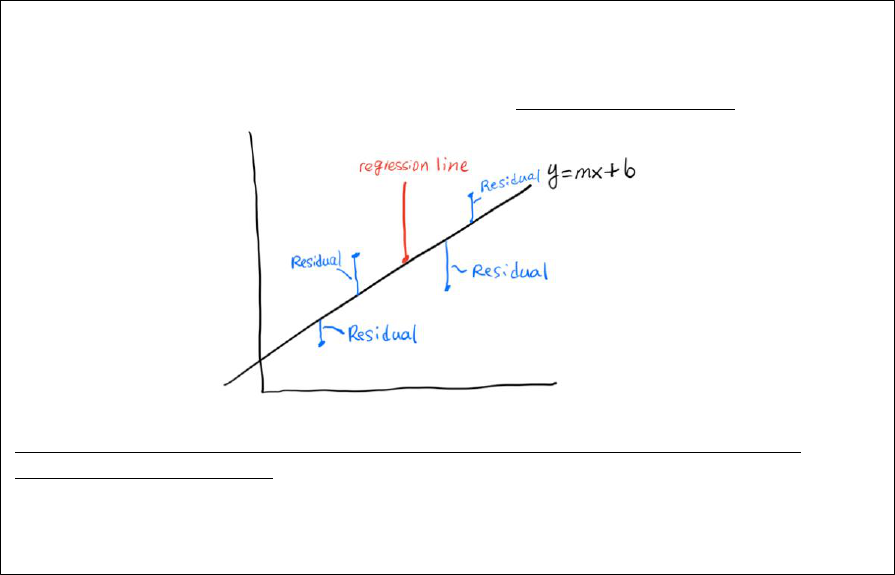
4.3 Linear Regression
Assumptions:
▪ Linearity: the relationship between dependent (graphed on y-axis) and independent
variabled (graphed on x-axis) should be approximately linear. This can be done by
creating a scatterplot in Excel.
▪ Independent observations: each pair of the independent and dependent variable
(x,y) is independent from other pairs.
▪ Normality of residuals: the residuals (the difference between the measured
dependent variable and the value predicted by the model given the independent
variable) from the regression model are normally distributed. This can be done
usimg Real Statistics add-in (section 3.1) “Reg” → “Multiple Linear Regression”
→ “Normality Test”.
▪ Constant variability of residuals (homoscedastic): the residuals should be
approximately constant for different values of the independent variable. This can be
done in Real Statistics “Reg” → “Multiple Linear Regression” → “Residuals
and Cook’s D”. Residuals with constant variability indicates that the residuals will
equally spread across the horizontal line of y = 0, without any other obvious
patterns.
Hypothesis for linear regression:
Linear regression follows the formula below:
▪ H
0
: the variation in Y is not explained by the model
▪ H
a
: a portion of variation in Y is explained by the model
Conduct linear regression in Excel:
14
1. You can run a regression through ‘Tools’, then ‘Data Analysis’ and selecting
‘Regression’.
2. For the ‘Input Y range’, click on the small box with the red arrow at the right end
of the entry area. On the main screen, click and drag your mouse over the entirety
of your dependent variable (the one whose values presumably depend on, or are
influenced by, the corresponding values of the independent variable)—this
essentially enters your range of data. Click the red area in the small box again,
which takes you back to the ‘Regression” screen and do the same thing for the
‘Input X range’ with your 2
nd
data column.
3. Among the output for this analysis, you will see “R Square/R
2
” which describes
the degree to which your regression line or linear model explains the variation in
your data, i.e., the goodness of fit (see the definition of R square in the box at the
next page). Also, the slope of the line or “Coefficients” for variables on the x-
axis, is the degree to which your x variable predicts the y variable – note: the
analysis will also assign a p-value to the slope term, indicating whether your
regression line slope is significantly different from zero.
4. When presenting your regression figure, a good approach would be to add R
2
,
the regression equation (and potentially p-value) along with your figure. When you
created the scatterplot, you can add regression line by double clicking the graph,
and select ‘Add Chart Element’ → ‘Trendline’. Right click the trendline on the
graph after it’s added, select ‘Format Trendline’. Under bottom right, you should
see options of ‘Display Equation on Chart’ and ‘Display R-squared value on
chart’.
What is R
2
(coefficient of determination)? You might notice that not all the data points directly overlap
with your regression line. Indeed, in science, most of the time, regression analysis will not capture all of
your data pattern. The distance between the actual value (y-value for each point) and predicted value (y-
value the regression line predicted given the x-value) is called residual error or a residual.
R
2
relates the proportion of variance in the dependent variable (response) that can be explained by
independent variable (predictor). R
2
ranges from 0 to 1, with 1 meaning that the model can explain 100% of
the relationship you observed, and vice versa. For example, if the R
2
is 0.35 for the regression line in the
figure above, it means that the variance in the (x variable) explains approximately 35% of the variance in
the (y variable).

15
Part 5
Real Statistics: non parametric tests
5.1 Wilcoxon Rank-Sum test
If the dependent variable is not from a normal distribution then you might avoid conducting a
two-sample t-test, instead you might choose a non-parametric alternative that does not have the
assumption of a normal distribution: one example of a nonparametric test is a Wilcoxon rank-
sum test (Mann-Whitney U test). The independence assumption from the t-test still applies to
Wilcoxon Rank-Sum test. Instead of comparing the mean of two samples like in a two-sample t-
test, the Wilcoxon Rank-Sum test compares the median (M) of two samples.
Conduct Wilcoxon Rank-Sum in Excel:
1. Open Real Statistics.
2. Under “Misc”, select “T-test and non-parametric Equivalents”.
3. Click the “+” sign next to “Input Range” to select one column of data you for
“Input Range 1” and “Input Range 2”. If you include the title (non-numerical) of
your column in the selection, make sure to check the box for “Column headings
included with data”.
4. In the “Options” box below, select the appropriate box for your t-test type (refer
back to section 4.2 if you are unsure the difference between “Two paired samples”
and “Two independent samples”); “One sample” is only used if you have one
group of data and want to compare to an existing value, in which case you should
enter the value you want to compare in “Hyp Mean/Median”.
5. Select “non-parametric” under “Test type”. Leave all checked options under
“Non-parametric test options” intact.
6. Either select an empty range for “Output Range” if you want to make the result
appear at your desirable location or leave it empty if you want the result to be in a
new worksheet. Click “OK”.
7. In the test output, you should be able to determine whether your two groups have
equal median or not by looking at the “p-norm” or “p-exact”.
2
2
“p-norm” and “p-exact” might be a little different depending on whether there will be ties in your data, since Wilcoxon Rank-Sum test uses rank
to compare the median between two groups. The mechanism is a little complicated so will not be covered here.
16
5.2 Kruskal-Wallis test
Like Wilcoxon Rank-Sum test, if the dependent variable is not from a normal distribution when
conducting an ANOVA, then we should choose a non-parametric alternative that does not have
assumption on the sample/population distribution called Kruskal-Wallis test. The independence
assumption from ANOVA still applies to Kruskal-Wallis test.
Hypothesis for Kruskal-Wallis test:
Like Wilcoxon Rank-sum test, the Kruskal-Wallis test compares the median (M) of three or
more samples.
▪ H
0
:
▪ H
a
:
Conduct Kruskal-Wallis in Excel:
1. Open Real Statistics.
2. Under “Anova”, select “One-factor ANOVA”.
3. Click the “+” sign next to “Input Range” to all groups of data organize by
columns. If you include the title (non-numerical) of your column in the selection,
make sure to check the box for “Column headings included with data”.
4. In the “Omnibus test options” below, select “Kruskal-Wallis”.
5. In the “Kruskal-Wallis follow-up options” below, select “Pairwise MW”, which
means pairwise Wilcoxon Rank-sum test (Mann-Whitney U test), but feel free to
try other options as well (or you can wait until your Kruskal-Wallis test returns a
significant p-value)!
6. Either select an empty range for “Output Range” if you want to make the result
appear at your desirable location or leave it empty if you want the result to be in a
new worksheet. Click “OK”.
7. In the test output, under “Kruskal-Wallis Test”, you should be able to determine
whether all your groups have equal median or not by looking at the “p-value” and
“sig”.
8. If the “p-value” is less than 0.05, proceed to section 6.3.

17
Part 6
Real Statistics: ANOVA and Post-hoc analysis
6.1 ANOVA
One-way ANOVA
A t-test can only compare means between two samples, so for a comparison of three or more
groups, we need to use ANOVA (Analysis of Variance). A one-way ANOVA indicates that all
the dependent variables are grouped by a single independent variable. One-way ANOVA can be
further divided into Model I ANOVA and Model II ANOVA, but for most cases in your classes,
you will use Model I ANOVA that will be explained below.
3
ANOVA is also included in the
Data Analysis add-on, but it requires you to have a similar number of individuals in equal group,
so it’s recommended to conduct ANOVA in “Real Statistics”.
Assumptions:
▪ Independence between and within groups: each observation in group one is not
associated with any observation in group two (between groups) or other
observations from the same group (within groups).
▪ The dependent variable must from a normal distribution: refer to section 3.2
for testing of normality (if the normality assumption is violated, then you might
consider using a non-parametric test).
▪ Equal variance between all dependent variables: see section 3.3 for testing of
homogeneity of variances.
Hypothesis for One-way ANOVA:
▪ H
0
:
▪ H
a
:
Optional: Why use ANOVA but not apply a series of multiple t-tests?
Instead of conducting an ANOVA, why don’t we just conduct many two-sample t-tests for each possible
combination (e.g., A ~ B, B ~ C…)? This is because every time we conduct a two-sample t-test, there is a chance
that we wrongfully conclude the result (i.e., the null hypothesis is true, called Type I error). That chance gets
significantly higher as we conduct more two-sample t-tests. Fortunately, many post-hoc analyses (section 6.2) have
adjusted the p-value based on the number of comparisons made so it significantly reduced the chance of making a
Type I error.
3
Model I analysis is also called fixed effects (the effects have known parameter values), while Model II analysis is called random-effects.
18
Conduct One-way ANOVA in Excel:
1. Open Real Statistics.
2. Under “Anova”, select “One Factor ANOVA”.
3. Click the “+” sign next to “Input Range” to all groups of data organize by
columns. If you include the title (non-numerical) of your column in the selection,
make sure to check the box for “Column headings included with data”.
4. In the “Omnibus test options” below, select “ANOVA”.
5. Either select an empty range for “Output Range” if you want to make the result
appear at your desirable location or leave it empty if you want the result to be in a
new worksheet. Click “OK”.
6. In the test output, under “ANOVA” table, you should be able to determine whether
all your groups have equal mean or not by looking at the “P value” of “Between
Groups”.
7. If the “P value” is less than 0.05, proceed to steps in section 6.2.
Two-way ANOVA
Two-way ANOVA measures the effect of two independent variables on a dependent variable. In
addition to this, the other difference with a One-way ANOVA is the interaction term or the
degree to which two independent variables have a combinatorial effect on the dependent
variable. A common way of design for Two-way ANOVA is called “Factorial Design”, and
that’s what we will cover in this part.
Assumptions:
▪ Independence between and within groups: each observation in group one is not
associated with any observation in group two (between groups) or other
observations from the same group (within groups).
▪ Each dependent variable must be from a normal distribution: refer to section
3.2 for testing of normality (if the normality assumption is violated, then you might
consider using a non-parametric test).
▪ Equal variance between all dependent variables: see section 3.3 for testing of
homogeneity of variances.

19
The data layout for the Factorial Design for Two-way ANOVA
Make sure your data table looks like this when proceeding with Two-way ANOVA in Excel:
Factor two level
Factor one level
1
2
3
…
a
1
X
111
X
211
X
311
X
a11
X
112
X
212
X
312
X
a12
X
113
X
213
X
313
X
a13
…
…
…
…
…
X
11n
X
21n
X
31N
X
a1N
2
X
121
X
221
X
321
X
a21
X
122
X
222
X
322
X
a22
X
123
X
223
X
323
X
a23
…
…
…
…
…
X
12n
X
22N
X
32N
X
a2N
3
X
131
X
231
X
331
X
a31
X
132
X
232
X
332
X
a32
X
133
X
233
X
333
X
a33
…
…
…
…
X
13n
X
23N
X
33N
X
a3N
…
…
…
…
…
…
b
X
1b1
X
2B1
X
3B1
X
aB1
X is the dependent variable, three subscripts are factor one level n, factor two level n, and the
order of that dependent variable in the combination of factor one level n and factor two level n.
Note: in Excel, the number of rows for a factor (factor two above) have to be the same to conduct
Two-way ANOVA.
Conduct Two-way ANOVA in Excel:
1. Open “Real Statistics”.
2. Make sure to have the table set in the same format in “The data layout for the
Factorial Design for Two-way ANOVA”.
3. Under “Anova”, select “Two Factor ANOVA”.
4. Click the “+” sign next to “Input Range” to all groups of data organize by columns
and row. Make sure you have equal number of rows for the factor grouped by row
(unfortunately, if you don’t you can’t run Two-way ANOVA in Excel). If you
include the title (non-numerical) of your column in the selection, make sure to
check the box for “Row/Column headings included with”.
5. In the “Analysis Type” below, select “ANOVA - Fixed”.
6. In the “Option for Excel format”, enter the number of rows in “Number of Rows
per Sample”.
20
7. Either select an empty range for “Output Range” if you want to make the result
appear at your desirable location or leave it empty if you want the result to be in a
new worksheet. Click “OK”.
8. In the test output, under “Two Factor ANOVA” table, you should be able to
separately determine to whether reject or fail to reject three null hypotheses by
looking at the “p-value” of “Rows” (factor grouped by row), “Columns” (factor
grouped by column), and “Inter” (interactions).
9. If the “p-value” is less than 0.05 for any of the three above, go back to step 3 and
select “Follow-up Two Factor Anova with Repl.” Or “Follow-up Two Factor
Anova without Repl.” Under “Select one of these options”, select the one that is
significant and click “OK”. This part will be expanded in more details later.
6.2 Post-hoc analysis for One-way ANOVA
Before getting to the meaning of “post-hoc”, let take a look at the hypothesis for ANOVA test
again.
Notice that if you reject the null hypothesis (p < 0.05), the alternative hypothesis only says that
“at least one pair of means are not equal”, it does not tell you which specific pair(s) is/are
different. For example, if you collected soil nutrient sample from 5 sites, with 20 samples from
each site, and your p-value is less than 0.05, the ANOVA tells you that at least the mean of one
pair of soil nutrient comparison is different, but never which one (e.g., site 1 ~ 2, site 3~ 5…).
This is when a post-hoc test can be useful in elucidating where specific differences lie.
Conduct Post-hoc of ANOVA in Excel:
1. Open “Real Statistics”.
2. Make sure that the p-value for ANOVA is less than 0.05.
3. Under “Anova”, select “One Factor ANOVA”.
4. Click the “+” sign next to “Input Range” to all groups of data organize by
columns. If you include the title (non-numerical) of your column in the selection,
make sure to check the box for “Column headings included with data”.
5. In the “ANOVA follow-up options”, select one of the tests, a commonly used
more conservative test is the “Tukey HSD”.
6. Either select an empty range for “Output Range” if you want to make the result
appear at your desirable location or leave it empty if you want the result to be in a
new worksheet. Click “OK”.
7. Depending on the test you selected in step 5, use “Tukey HSD” as an example, in
the test output, under “Q TEST” table, you should be able to determine which
comparison(s) is statistically significant by looking at the “p-value” and “group 1”
and “group 2” for that row.
21
6.3 Post-hoc analysis for Kruskal-Wallis
If there is a post-hoc for ANOVA, you can imagine there will be one for Kruskal-Wallis.
Conduct post-hoc of Kruskal-Wallis in Excel:
1. Open “Real Statistics”.
2. Under “Anova”, select “One Factor ANOVA”.
3. Click the “+” sign next to “Input Range” to all groups of data organized by
columns. If you include the title (non-numerical) of your column in the selection,
make sure to check the box for “Column headings included with data”.
4. In the “Kruskal-Wallis follow-up options”, select one of the options, a commonly
used method is “Pairwise MW”, which means Pairwise Wilxoxon Rank-Sum
(Mann-Whitney) tests, the p-value will be adjusted so the chances of making Type
I error are reduced.
5. Either select an empty range for “Output Range” if you want to make the result
appear at your desirable location or leave it empty if you want the result to be in a
new worksheet. Click “OK”.
6. In the test output, under “Kruskal-Wallis Test”, you should be able to determine
what combination(s) will have different median by looking at the “p-value”, and
“group 1” and “group 2” for that row.
6.4 Additional helpful tests in Real Statistics
Due to the limited page, many other statistical tests won’t be covered by this document, but they
are available in Real Statistics. Below are some examples:
Multiple Linear Regression in “Reg”: when you plot one continuous dependent variable
against multiple continuous independent variable (multiple x).
Polynomial Regression in “Reg”: when the relationship between the dependent variable and
independent variable is not linear (e.g., x increases more with the same increase in y).
Poisson Regression in “Reg”: Poisson regression is often used when you have count data
(integer, ≥ 0) as the dependent variable. Count data often follows Poisson distribution that often
has higher frequency on the low end of the distribution, not normal distribution. But the variance
should not be greater than the mean in Poisson Regression.
Chi-Squared test for Independence in “Misc”: tests if there is a relationship between two
categorical variables.
Goodness of fit in “Misc”: tests if a categorical variable follows the hypothesized distribution.
